`

HEADWAY DISTRIBUTION FOR NH-8 TRAFFIC AT VAGHASI VILLAGE LOCATION

Dr. L. B. ZalaAssociate Professor,

Civil Engineering Department,Birla Vishvakarma Mahavidyalaya Engineering College,

Vallabh Vidyamagar, Indialbzala@yahoo.co.in

Kevin B. ModiM.Tech (Civil) Transportation System Engineering (Student),

Civil Engineering Department,Birla Vishvakarma Mahavidyalaya Engineering College,

Vallabh Vidyamagar, Indiakevin_modi@yahoo.co.in

Dr. (Mrs.) T. A. DesaiProfessor and Head of Mathematics Department,

Birla Vishvakarma Mahavidyalaya Engineering College,Vallabh Vidyamagar, India

tadesaibvm@gmail.com

Aakar N. RogheliaAssistant Professor, Mathematics Department,

Birla Vishvakarma Mahavidyalaya Engineering College,Vallabh Vidyamagar, India

aakarkhyati@gmail.com

Abstract- The properties of vehicle time headways are fundamentals in many traffic engineering applications, such as capacity and level of service studies on highways, unsignalized intersections, and roundabouts. In addition, the vehicle generation in traffic flow simulation is usually based on some theoretical vehicle time headway model. The statistical analysis of vehicle time headways has been inadequate in three important aspects: 1) There has been no standard procedure to collect headway data and to describe their statistical properties. 2) The fit goodness tests have been either powerless or infeasible. 3) Test results from multi sample data have not been combined properly.In this paper describe the study conducted on two lane mid block section of National Highway-8 (NH-8), between Ahmedabad and Vadodara, at Vaghasi village to evaluate basic traffic flow parameters. Data collection was done using Video Recording Technique. The headway data extracted and compared with different type of vehicles in traffic stream.

Keywords- Headway; headway distribution; capacity; PCUs.

I. INTRODUCTION

The time headway between vehicles is an important microscopic flow characteristic that affects the safety, level of service, driver behavior and capacity of transportation systems. The capacity of the system is governed primarily by the minimum time headway ant the time headway distribution under capacity flow conditions.

The elapsed time between pairs of vehicles is defined as the time headway. A microscopic view of traffic flow is shown in figure 1, as several vehicles traverse a length of roadway in single file for a certain period of time.

II. LITERATURE REVIEW

A convenient way to describe the inherent variability within a traffic stream is to consider it as a stochastic process,

to examine the headways between vehicles in the stream, and to search for statistical distribution that describe the frequencies of occurrence of headways. In normal terms, it is defined to be the time difference between the same points (e.g. The front bumper) on two consecutive vehicles as they pass an observation point on the road. This definition holds for single or multilane traffic. An important qualification from this definition is that it explicitly ignores the physical length of the vehicles. Vehicles are regarded points only. Then, under this definition the reciprocal of the mean headway is equal to mean flow rate.

Figure 1. A microscopic view of traffic flow

Source: May, A. D. “Traffic flow fundamentals” Prentice hall, 1990 , pp-12

A. Headway Method

The time interval between successive vehicles in a traffic stream is used for determining the volume of traffic.

Traffic volume, (Q) Q = 3600 (1) Headway (h)

13-14 May 2011 B.V.M. Engineering College, V.V.Nagar,Gujarat,India

National Conference on Recent Trends in Engineering & Technology

`

Where, Q = measured in vehicles per hourh = time headway in seconds

Consider a stream of traffic in which only two categories viz. cars, trucks, and scooters are present. For this Guinn, Reilly and Seifert has suggested following basic equation.Then, basic equation of headway method is:

E = (hm / hc –c) (2)t

Where, hc = time headway between two cars in seconds for an “all cars” streamhm = time headway between two vehicles in mixed flow stream (seconds)c = proportion of cars in the mixed streamt = proportion of trucks in the mixed streams = proportion of scooters in the mixed streamE = PCU of trucks

The above equation gives a simple basis for determination of PCU factors when only cars, trucks, scooters and another type of vehicles are present. All that is needed is to measure the average time headway of a sample of all car samples and the average time headway of the mixed traffic. Duration of at least one hour is desirable. The value so obtained is valid only for the flow and speed conditions prevailing. The method is appropriate for plain terrain and for low levels of service. The method does not consider the overtaking phenomenon where faster vehicles tend to overtake the slower ones.

B. Classification Of Headway Distribution

One can observe three types of flow in the field.1) Low Volume Flow:

Headway follow a random process as there is no intersection between the arrivals of two vehicles.

The arrival of one vehicle is independent of the arrival of other vehicle.

The minimum headway is governed by the safety criteria.

A negative exponential distribution can be used to model such flow.

2) High Volume Flow

This is characterized by ‘near’ constant headway. The flow is very high and is near to capacity. The mean is very low and so is the variance. A normal distribution can be used to model such

flow.

3) Intermediate Flow

Some vehicle travel independently and some vehicle has interaction.

More difficult to analyzed and has more application in the field.

Pearson Type III distribution can be used which is a very general case of negative exponential distribution and normal distribution.

C. Negative Exponential Distribution

The negative exponential distribution can be used to illustrate this headway state. For time headways to be truly random, two conditions to be met. Firstly, any point in time is likely to have a vehicle arriving as is any other point in time. Secondly, the arrival of one vehicle at a point in time does not affect the arrival time of any other vehicle.

The negative exponential distribution can be derived from the Poisson count distribution. The particular distribution can be indicated by the following form,

P (x) = (m * e-m)/ x! (3)

Where, P (x) = Probability of arrival of x vehicles in any interval of t sec m= (average rate of arrival) * (time interval)

Let us consider the special case when there is no vehicle. x=0

P( 0 ) = e-m (4)

This means if there is no vehicle then the individual time headway must be equal or greater than t.Therefore,

P (0) = P (h ≥t) (5)

P (h ≥t) = e-m (6)

Now m is defined as the avg. no. of vehicles arriving in time interval t. The hourly flow rate is V and t in seconds.Then,

m = (V/3600) t (7)

P (h ≥t) = e-(V/3600) t (8)

The mean time headway can be (μ) determined easily so,

P (h ≥t) = e-t/μ (9)

To calculate probability of a time headway between t and t+Δt

P (t ≤ h ≤ t + Δt) = P (h ≥ t)-P (h≥ t + Δt) (10)

Following the above mentioned procedure it is possible to fit this distribution into different flow levels to show the characteristics of the distribution. The theoretical results are superimposed on the measured time headway distribution. Careful study will give some characteristics of the random distribution to observed one. Some of the important observations are:

13-14 May 2011 B.V.M. Engineering College, V.V.Nagar,Gujarat,India

National Conference on Recent Trends in Engineering & Technology

`

The random distribution has a characteristic of smallest headways occurring most likely, probabilities continuously decrease with the increase with time headway.

The comparison is best under lowest flow level.

D. Pearson type III Distribution

The intermediate headway state lies between the two boundary conditions random, constant headway states. This is the situation encountered almost every day. In this section it is tried to describe Pearson type III distribution by which we can easily illustrate this headway state.

Pearson type III distribution is a generalized mathematical model approach.

Where, λ is parameter that is function of µ, K, and α;K = user specified parameter between 0 and ∞α = user selected parameter greater than 0 and called as the shift parameter = gamma function ( K = (K-1)!)

Then, (11)

Probability of headway lying t and t+δt is

(12)

Approximating,

(13)

Some of the important observations are The probability of the theoretical and measured

distribution is most inconsistent when time headways between 1 and 4 sec.

The comparison between this and measured distribution at four flow levels indicates that qualitatively the two are about the same.

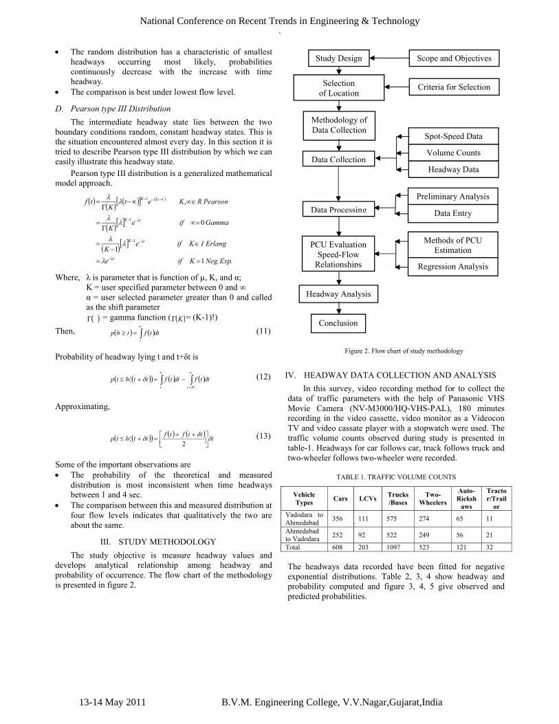
III. STUDY METHODOLOGY

The study objective is measure headway values and develops analytical relationship among headway and probability of occurrence. The flow chart of the methodology is presented in figure 2.

Figure 2. Flow chart of study methodology

IV. HEADWAY DATA COLLECTION AND ANALYSIS

In this survey, video recording method for to collect the data of traffic parameters with the help of Panasonic VHS Movie Camera (NV-M3000/HQ-VHS-PAL), 180 minutes recording in the video cassette, video monitor as a Videocon TV and video cassate player with a stopwatch were used. Thetraffic volume counts observed during study is presented in table-1. Headways for car follows car, truck follows truck and two-wheeler follows two-wheeler were recorded.

TABLE 1. TRAFFIC VOLUME COUNTS

Vehicle Types

Cars LCVsTrucks/Buses

Two-Wheelers

Auto-Ricksh

aws

Tractor/Trail

orVadodara to Ahmedabad

356 111 575 274 65 11

Ahmedabad to Vadodara

252 92 522 249 56 21

Total 608 203 1097 523 121 32

The headways data recorded have been fitted for negative exponential distributions. Table 2, 3, 4 show headway and probability computed and figure 3, 4, 5 give observed and predicted probabilities.

..1

1

0

,

1

1

1

ExpNegKife

ErlangIKifeK

GammaifeK

PearsonRKetK

tf

t

tK

tK

tK

dttfthpt

dttfdttftthtpttt

t

ttftftthtp

2

Study Design

Selectionof Location

Methodology of Data Collection

Scope and Objectives

Criteria for Selection

Spot-Speed Data

Volume Counts

Headway DataData Collection

Data Processing

Preliminary Analysis

Data Entry

PCU Evaluation Speed-Flow

Relationships

Headway Analysis

Conclusion

Methods of PCU Estimation

Regression Analysis

13-14 May 2011 B.V.M. Engineering College, V.V.Nagar,Gujarat,India

National Conference on Recent Trends in Engineering & Technology

`

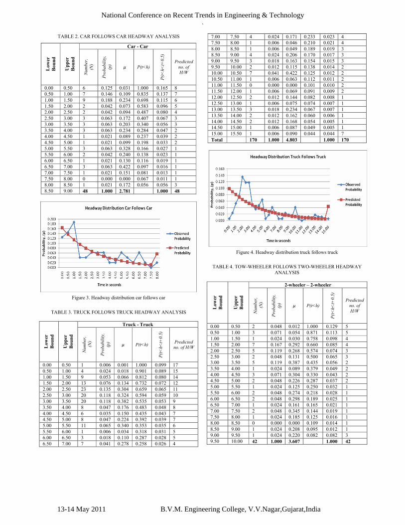
TABLE 2. CAR FOLLOWS CAR HEADWAY ANALYSIS

Car - CarL

ower

Bou

nd

Up

per

Bou

nd

Num

ber,

(N)

Pro

babi

lity

, (p

) µ P(t<h)

P(t

<h<

t+0.

5)

Predicted no. of H/W

0.00 0.50 6 0.125 0.031 1.000 0.165 80.50 1.00 7 0.146 0.109 0.835 0.137 71.00 1.50 9 0.188 0.234 0.698 0.115 61.50 2.00 2 0.042 0.073 0.583 0.096 52.00 2.50 2 0.042 0.094 0.487 0.080 42.50 3.00 3 0.063 0.172 0.407 0.067 33.00 3.50 3 0.063 0.203 0.340 0.056 33.50 4.00 3 0.063 0.234 0.284 0.047 24.00 4.50 1 0.021 0.089 0.237 0.039 24.50 5.00 1 0.021 0.099 0.198 0.033 25.00 5.50 3 0.063 0.328 0.166 0.027 15.50 6.00 2 0.042 0.240 0.138 0.023 16.00 6.50 1 0.021 0.130 0.116 0.019 16.50 7.00 3 0.063 0.422 0.097 0.016 17.00 7.50 1 0.021 0.151 0.081 0.013 17.50 8.00 0 0.000 0.000 0.067 0.011 18.00 8.50 1 0.021 0.172 0.056 0.056 38.50 9.00 48 1.000 2.781 1.000 48

Figure 3. Headway distribution car follows car

TABLE 3. TRUCK FOLLOWS TRUCK HEADWAY ANALYSIS

Truck - Truck

Low

erB

oun

d

Up

per

Bou

nd

Num

ber,

(N

)

Pro

babi

lity

, (p

) µ P(t<h)

P(t

<h<

t+0.

5)

Predictedno. of H/W

0.00 0.50 1 0.006 0.001 1.000 0.099 170.50 1.00 4 0.024 0.018 0.901 0.089 151.00 1.50 9 0.053 0.066 0.812 0.080 141.50 2.00 13 0.076 0.134 0.732 0.072 122.00 2.50 23 0.135 0.304 0.659 0.065 112.50 3.00 20 0.118 0.324 0.594 0.059 103.00 3.50 20 0.118 0.382 0.535 0.053 93.50 4.00 8 0.047 0.176 0.483 0.048 84.00 4.50 6 0.035 0.150 0.435 0.043 74.50 5.00 8 0.047 0.224 0.392 0.039 75.00 5.50 11 0.065 0.340 0.353 0.035 65.50 6.00 1 0.006 0.034 0.318 0.031 56.00 6.50 3 0.018 0.110 0.287 0.028 56.50 7.00 7 0.041 0.278 0.258 0.026 4

7.00 7.50 4 0.024 0.171 0.233 0.023 47.50 8.00 1 0.006 0.046 0.210 0.021 48.00 8.50 1 0.006 0.049 0.189 0.019 38.50 9.00 4 0.024 0.206 0.170 0.017 39.00 9.50 3 0.018 0.163 0.154 0.015 39.50 10.00 2 0.012 0.115 0.138 0.014 210.00 10.50 7 0.041 0.422 0.125 0.012 210.50 11.00 1 0.006 0.063 0.112 0.011 211.00 11.50 0 0.000 0.000 0.101 0.010 211.50 12.00 1 0.006 0.069 0.091 0.009 212.00 12.50 2 0.012 0.144 0.082 0.008 112.50 13.00 1 0.006 0.075 0.074 0.007 113.00 13.50 3 0.018 0.234 0.067 0.007 113.50 14.00 2 0.012 0.162 0.060 0.006 114.00 14.50 2 0.012 0.168 0.054 0.005 114.50 15.00 1 0.006 0.087 0.049 0.005 115.00 15.50 1 0.006 0.090 0.044 0.044 7Total 170 1.000 4.803 1.000 170

Figure 4. Headway distribution truck follows truck

TABLE 4. TOW-WHEELER FOLLOWS TWO-WHEELER HEADWAY ANALYSIS

2-wheeler – 2-wheeler

Low

erB

oun

d

Up

per

Bou

nd

Num

ber,

(N

)

Pro

babi

lity

, (p

) µ P(t<h)

P(t

<h<

t+0.

5)

Predictedno. of H/W

0.00 0.50 2 0.048 0.012 1.000 0.129 50.50 1.00 3 0.071 0.054 0.871 0.113 51.00 1.50 1 0.024 0.030 0.758 0.098 41.50 2.00 7 0.167 0.292 0.660 0.085 42.00 2.50 5 0.119 0.268 0.574 0.074 32.50 3.00 2 0.048 0.131 0.500 0.065 33.00 3.50 5 0.119 0.387 0.435 0.056 23.50 4.00 1 0.024 0.089 0.379 0.049 24.00 4.50 3 0.071 0.304 0.330 0.043 24.50 5.00 2 0.048 0.226 0.287 0.037 25.00 5.50 1 0.024 0.125 0.250 0.032 15.50 6.00 2 0.048 0.274 0.218 0.028 16.00 6.50 2 0.048 0.298 0.189 0.025 16.50 7.00 1 0.024 0.161 0.165 0.021 17.00 7.50 2 0.048 0.345 0.144 0.019 17.50 8.00 1 0.024 0.185 0.125 0.016 18.00 8.50 0 0.000 0.000 0.109 0.014 18.50 9.00 1 0.024 0.208 0.095 0.012 19.00 9.50 1 0.024 0.220 0.082 0.082 39.50 10.00 42 1.000 3.607 1.000 42

13-14 May 2011 B.V.M. Engineering College, V.V.Nagar,Gujarat,India

National Conference on Recent Trends in Engineering & Technology

`

Figure 5. Headway distribution two-wheeler follows two-wheeler

V. CONCLUSION AND RECOMMENDATIONS

The following conclusion can be drawn from tabular data and plot.

Headway data for car follows negative distribution within range from 1.00 sec to 4.50 sec with µ is 2.781 sec.

Headway data for truck follows negative distribution within range from 2.50 sec to 14.50 sec with µ is 4.803 sec.

Headway data for two-wheeler follows negative distribution within range from 1.50 sec to 8.00 sec with µ is 3.607 sec.

The headway follows negative distribution up to 14.50 sec in the heterogeneous traffic stream.

The detailed headway data for all vehicles can be studied. The headway data should be used for capacity level of service analysis and evaluation of PCUs.

REFERENCES[1] Huber, M. J. (1982), “Estimation of Passenger Car Equivalents of

Trucks in Traffic Stream”, Transportation Research Record No. 869, Washington, D. C., pp. 60-70.

[2] Kadyali, L. R. and Lal, N. B. (2007), “Traffic Engineering and Transport Planning”, Khanna Publishers, Delhi-6.

[3] Kremmes, R. A. (1987), and Crowly, K. W., “Passenger Car Equaivalents for Trucks on Level Freeway Segments”, Transportation Research Record (1901), TRB, National Research Council, Washington, D. C., pp. 10-16.

[4] May, A. D. (1990), “Traffic Flow Fundamentals”, Prantice Hall, Englewood Cliffs, New Jersey.

[5] May, A. D. (1990), “Traffic flow fundamentals” Prentice hall, pp. 11-20.

[6] Mathew, T. V. and Krishna Rao, K. V. K. (2009), “Modelling Traffic Characteristics”, www.nitropdf.com/professional.

[7] Road User Cost Study in India (1982), Final Report, Central Road Research Institute, New Delhi.

[8] Transportation Research Board (TRB) (1965), Highway Capacity Manual, Special Report 87.

[9] Werner, A. and Morall, J. F. (1976), “Passenger Car Equivalences of Trucks, Buses, and Recreational vehicles for Two Lane Rural Highways”, Transportation Research Record 615, National Academic of Sciences, Washington, D. C.

[10] Zala, L. B. (1994), “Traffic Flow Analysis on Heavily Trafficked Highway”, Unpublished Dissertation Report, transportation Engineering Section, Civil Engineering Department, Roorkee University, Roorkee.

13-14 May 2011 B.V.M. Engineering College, V.V.Nagar,Gujarat,India

National Conference on Recent Trends in Engineering & Technology