Heads I win, tails you lose:

asymmetric taxes, risk taking, and

innovation⇤

James F. Albertus Brent Glover Oliver Levine

Carnegie Mellon University Carnegie Mellon University Univ. of Wisconsin-Madison

October 2018

ABSTRACT

When multinationals face lower tax rates abroad than in the US, transfer pricing

strategies generate an asymmetry in the tax rates on a project’s profits and losses.

We show that the tax savings from transfer pricing can be expressed as a long position

in a call option. We use a model to show that this transfer pricing call option leads

a firm to choose riskier and larger projects than it would otherwise. Thus, transfer

pricing strategies do not simply reduce a firm’s taxes, they can influence the scale and

types of projects undertaken.

⇤We gratefully acknowledge valuable comments from Kose John (discussant), Julian Kolm (discussant)

as well as seminar participants at the University of British Columbia, Carnegie Mellon University, the Third

Annual Young Scholars Finance Consortium, and the 2018 European Finance Association Annual Meeting.

Albertus: Tepper School of Business, Carnegie Mellon University, 5000 Forbes Avenue, Pittsburgh, PA

15213, albertus@cmu.edu.Glover: Tepper School of Business, Carnegie Mellon University, 5000 Forbes Avenue, Pittsburgh, PA 15213,

gloverb@andrew.cmu.edu.Levine: Finance Department, Wisconsin School of Business, University of Wisconsin-Madison, 975 University

Ave, Madison, WI 53706, oliver.levine@wisc.edu

1 Introduction

The high level of the statutory corporate income tax rate in the US, relative to that

of many developed economies, has received significant attention as a driving force behind

US multinationals’ business decisions. In the context of domestically operating firms, it has

long been recognized that taxes can influence a firm’s attitude towards risk (e.g., Domar and

Musgrave (1944); Green and Talmor (1985); Smith and Stulz (1985)). In spite of this, there

has been little attention paid to how firms’ foreign operations and the di↵erences in US and

foreign corporate tax rates may a↵ect the risk-taking of US firms.

In this paper, we show that the relatively high US tax rate, along with the ability of firms

to shift intangible capital across their global operations at discounted transfer prices, can

a↵ect the riskiness and scale of projects undertaken by US firms.1 For example, consider a

firm that develops intangible capital in the US. The expenses associated with the development

provides a valuable deduction against the firm’s US income that is taxed at a relatively high

US rate. In practice, the firm can use transfer pricing to move the intangible capital to

its foreign subsidiary at a price below its fair market value, shifting overseas the profits

generated by these assets. These profits are then taxed at relatively low foreign rates. We

show that typical transfer pricing strategies produce an asymmetry in the tax rates faced on

the gains and losses of a project with transferable capital. This generates convexity in the

after-tax payo↵s of these projects. Facing convex payo↵s, firms have incentive to increase

the riskiness and scale of these projects with transferable capital.

We use a model of a firm’s joint decision of project risk and scale to illustrate how di↵er-

ential tax rates and transfer pricing strategies firm policies. The model shows that a transfer

pricing strategy can be expressed as a long position in a call option on the development

of transferable capital or intellectual property. This call option component of the after-tax

payo↵ leads the firm to choose a project that is larger and riskier. We show that, somewhat

1Pomerleau (2017) reports that, as of 2017, the US has the fourth highest statutory corporate income

tax rate in the world. While the Tax Cuts and Jobs Act of 2017 reduced the US federal corporate tax rate

from 35% to 21%, it remains much higher than those in tax havens. For instance, Bermuda does not tax

corporate income.

1

surprisingly, an increase in the US tax rate can lead to an increase in the choice of project

scale and risk. Furthermore, we show that under certain conditions this can lead the firm

to invest more in a project than it would in an alternative case of zero taxes. The model

highlights the relevance of a firm’s other taxable income and the di↵erence in US and foreign

tax rates for the choice of project scale and risk.

We then empirically test these predictions for the relationship between corporate tax

rates and firm risk taking. Using geographic segment data, we construct a panel of the

foreign operations of US firms for the period 1998–2015. We follow the prior literature in

using the volatility of firm profitability as a proxy for corporate risk taking (John, Litov,

and Yeung (2008)). With this sample, we perform two sets of analyses.

In our first approach, we consider the simple correlation between the tax convexity and

risk taking. We find that the tax convexity and risk taking are positively related, as predicted

by the model. A natural concern is that this correlation is driven by selection. For example,

young tech firms may have both volatile cash flows and operations in tax havens. We

evaluate this concern by controlling for age and including industry fixed e↵ects. The positive

association between the tax convexity and risk taking remains.

As a second approach, we consider the e↵ect of major foreign tax changes. The advantage

of this type of analysis is that it allows us to assess the dynamics of the e↵ect of the tax

convexity on risk taking. It also allows us to examine whether our e↵ect is driven by trends

in the treatment (firms subject to a major foreign tax change) or control (firms not subject to

such a change) group prior to treatment. The estimates indicate that firms promptly adjust

their risk taking following treatment and do not anticipate major tax changes. While this

setting remains an approximation of the experimental ideal, the latter result is consistent

with the notion that changes in tax convexity cause firms to adjust their risk taking. Broadly

speaking, our results from both approaches are consistent with the prediction that the tax

convexity generates the incentive for multinationals to undertake riskier projects.

It has long been recognized in the corporate finance literature that features of the cor-

porate tax code can make the relationship between a firm’s taxable income and its tax

2

liability nonlinear. In particular, prior work has focused on two features—a progressive tax

rate schedule and the limited ability to utilize loss carryforwards—that make a firm’s tax

liability a convex function of its taxable income.2

Smith and Stulz (1985) show that when a firm faces a convex tax liability, it can reduce

its expected tax liability and increase firm value by hedging or engaging in other activities

that reduce the volatility of its taxable income. They also note that taxes may give firms a

motive to hedge in order to increase their debt capacity.3 Graham and Smith (1999) estimate

tax liability functions for a sample of Compustat firms and find convexity in about half of

their sample. Graham and Rogers (2002) empirically find firms hedge in order to increase

debt capacity but do not find evidence of hedging in response to tax function convexity.4

Green and Talmor (1985) and Majd and Myers (1985) show that the government’s tax

claim on a firm’s profits can be viewed as a call option. The firm has a short position in this

call option and therefore would like to reduce the volatility of taxable income to reduce its

expected tax liability. Green and Talmor (1985) show that this convex tax liability reduces

the firm’s incentive to take on risk, giving incentive to underinvest and engage in conglom-

erate, diversifying mergers.5 We show that in the international setting, this prediction for

corporate risk taking may be reversed. Favilukis, Giammarino, and Pizarro (2016) and

Schiller (2015) study how corporate taxes and the structure of tax loss carryforwards a↵ect

the riskiness of equity returns. Ljungqvist, Zhang, and Zuo (2017) use changes in the level

of corporate tax rates across US states to study how tax rates a↵ect firm risk-taking. They

find that the average firm in their sample reduces its risk-taking in response to a state-level

tax increase, but does not increase risk-taking in response to a cut. Becker, Johannesen, and

Riedel (2018) studies the relation between taxes and the allocation of risk within the firm.

In contrast, our focus is on firms’ overall risk taking, not its distribution.

2See Graham (2006) for a review of the literature on taxes and corporate finance decisions.

3See also Ross (1996) and Leland (1998).

4Using survey data on firms’ usage of derivatives, Nance, Smith, and Smithson (1993) find that firms

facing a more convex tax function, proxied by the amount of net operating losses, are more likely to hedge.5More recently, Langenmayr and Lester (2017) and Ljungqvist, Zhang, and Zuo (2017) provide empirical

evidence consistent with Green and Talmor (1985). Osswald and Sureth-Sloane (2017) shows that country

risk weakens the association between tax loss o↵sets and risk taking.

3

2 Transfer pricing of intangible capital

Large firms are often comprised of a set of legally distinct entities. To be concrete,

consider the case of a pharmaceutical company headquartered in the US that is developing a

drug for sale in both the US and foreign markets. Suppose the firm has an Irish subsidiary.

Typically, the Irish subsidiary will be separately incorporated from the US parent. Legal

contracts define the relationships among the entities that constitute the firm. Often, the US

parent will wholly own the equity of the Irish subsidiary.

As a consequence, property must be sold (or similarly legally transferred, but not given)

from the parent to the Irish subsidiary. IRS regulations require that these transfers occur

at“arm’s length” prices. In other words, if the Irish subsidiary handles the firm’s non-US sales

of the drug, it must pay the US parent the market value of the right to sell the drug abroad.

If the parent bears the full risk of developing the drug, the payment from the subsidiary to

the parent must be higher than if the subsidiary shares in the risk of development.

Although the transfers are required to take place at market prices, the item being trans-

ferred may be highly di↵erentiated. As such, a market price may be di�cult to determine.

Following the example, the value of the drug developed by the pharmaceutical company’s

US parent may be genuinely ambiguous if it is new and lacks a counterpart that is sold in

the market. Similarly, the share of the risk borne by the Irish subsidiary in developing the

drug may be di�cult to precisely quantify in economic terms.

In practice, if the development of the drug looks unlikely to produce a viable product, the

US parent may choose to record the full development expense in the US, shielding its other

domestic taxable income from the relatively high US corporate income tax rate. Conversely,

if the drug’s development looks primising, the parent may cost share the right to sell the

drug abroad to the Irish subsidiary at price below its market value. The profits that accrue

at the Irish subsidiary would then be subject to the relatively low Irish corporate tax rate.

Cost sharing agreements are generally not publicly available. Consequently, the degree to

which transfer pricing undercuts the conceptual arm’s length standard is di�cult to ascertain.

However, Bernard et al. (2006) suggests it is substantial for US multinationals, particularly

4

for di↵erentiated goods, where they estimate it ranges from 52.8% to 66.7%.6 Moreover,

anecdotally, the IRS rarely challenges cost sharing agreements. As a result, firms plausibly

transfer intangible capital on favorable terms.

3 Model

A multinational firm can undertake a new project in which it jointly chooses the scale

and riskiness. Specifically, the firm chooses an amount C to spend on R&D and project risk

�. The project produces intellectual property (IP), which can be transferred and utilized by

all of the firms operations. The pre-tax value of the project’s IP is XC↵, where ↵ < 1,

log(X) ⇠ N (µ(�), �2), (1)

and

µ(�) = µ+ (�1 � �2�)�. (2)

This specification for µ(�) implies that there is a value of � that maximizes the expected

value of X and therefore the expected pre-tax payo↵ on the project.

In the event that the R&D investment is successful (XC↵ � C > 0), the firm can apply

this IP to all of its operations. We assume a fraction ✓ of the firm’s operations are abroad,

and the income from these operations is subject to a foreign tax rate of ⌧F . The remaining

1 � ✓ of operations are located in the US and subject to a US tax rate of ⌧US. All of the

R&D is performed in the US and recorded as a US expense for tax purposes. The project

payo↵s before taxes are ✓XC↵ abroad and (1� ✓)XC↵ � C in the US.

6For commodities, they estimate a price reduction of 8.8% to 17.6%. Cristea and Nguyen (2016) find

similar magnitudes for tangible goods transferred within Danish firms. Davies et al. (2018) find intrafirm

prices are 11% lower than market prices for French firms.

5

3.1 No taxes

With no taxes, the firm’s problem is simply

maxC,�

E[XC↵ � C], (3)

subject to the constraint C > 0, � > 0. With our assumption of lognormality for X, the

first-order condition for � is

(�1 � 2�2� + �)eµ+�1���2�2+�2

2 = 0, (4)

which gives the optimal volatility choice

� =�1

2�2 � 1. (5)

The optimal choice of C is given by

C =⇣↵eµ+(�1��2�)�+

�2

2

⌘ 11�↵

(6)

The NPV of the project is

NPV = �C + C↵eµ+(�1��2�)�+�2

2 (7)

3.2 Constant single tax rate

If the firm faces a single tax rate of ⌧ for any level or source of income, then the optimal

choice of scale C and risk � for the project is the same as in the case of no taxes. The firm’s

problem is

maxC,�

E[(1� ⌧)(XC↵ � C)]. (8)

While taxes here will a↵ect the NPV of the project, the first order conditions are the same

as in the zero tax case and so the optimal choices of C and � are unchanged by the presence

6

of taxes.

3.3 U.S. and foreign taxes with transfer pricing

Now we consider the case where the firm faces a di↵erent tax rate on its foreign operations

(⌧F ) than domestic operations (⌧US). Throughout, we assume that the US corporate tax rate

exceeds the foreign rate, ⌧US > ⌧F , giving the firm incentive to shift profits from the US to

the lower tax foreign jurisdictions.

We assume that the R&D is performed entirely in the U.S., resulting in an expense for

U.S. tax purposes. This assumption is loosely consistent with the fact that US multinationals

perform more than 80% of their R&D in the US.7 However, the intangible capital resulting

from the R&D has value for both the domestic and foreign operations. We use ✓ to denote

the fraction of foreign operations. That is, the pre-tax value of the intangible capital is

✓XC↵ for the foreign operations and (1� ✓)XC↵ for the domestic operations.

In the event that the project has a positive outcome where XC↵ � C > 0, we assume

that the firm can transfer the intangible capital to its foreign operations at price p(X,C, ✓).

The firm is assumed to be able to transfer this intangible capital at a discount of its fair

market value:

p(X,C, ✓) < ✓XC↵. (9)

The case in which the intangible capital is transferred at a price of ✓C corresponds to

one where the R&D expense is allocated proportionally: ✓ fraction of the firm’s operations

are abroad and it allocates ✓ fraction of its R&D expense to these foreign operations. In

computing comparative statics from the model, we assume the firm uses this proportional

allocation such that its transfer price is p(X,C, ✓) = ✓C. Given the parameter values listed

in Table 1, this implies a relatively conservative average discount of 9% in the transfer price.8

7In 2015 (the most recent year for which finalized data are available at the time of writing), the US par-

ents of multinational firms performed $277,787 million in R&D. Their majority-owned subsidiaries performed

$56,096 million. Majority owned subsidiaries represent the bulk of US multinationals’ foreign operations, ac-

counting for roughly 86% of all foreign subsidiaries’ sales ($5,950,947 million of $6,871,187 million) (Bureau of

Economic Analysis (2018)).8That is, for the optimally chosen � and C, the transfer price to market value ratio is

✓CE(✓XC↵) = 0.91.

7

We assume the firm has other contemporaneous US income from operations, Y � 0, and

this is known in advance of the project decision. In this case, if the project generates a loss

(XC↵�C < 0) that exceeds the other taxable income Y , then the full amount of the project

loss isn’t captured for tax purposes. If we ignore the ability to carry forward losses, then the

project’s payo↵ can be divided into three regions:

• Region 1: XC↵ � C < �Y

In this case, the project’s losses exceed the other income Y and so the project reduces

the firm’s US taxes paid by ⌧USY . In other words, the firm is unable to capture the

full loss for tax purposes. The payo↵ on the project is (XC↵ � C) + ⌧USY .

• Region 2: �Y XC↵ � C 0

In this case, the project’s losses are less than the other US income Y and so the full

loss reduces the firm’s taxable income. With the project loss, the firm’s tax liability is

lower by ⌧US(XC↵ � C)

• Region 3: XC↵ � C > 0

In this case the project is profitable and the total after-tax payo↵ is

XC↵ � C � ⌧US[(1� ✓)XC↵ + p(X,C, ✓)� C]� ⌧F [✓XC↵ � p(X,C, ✓)] (10)

The firm chooses the scale C and the riskiness � of the project to maximize the expected

after-tax payo↵. Combining the payo↵s across the three regions described above, we can

write the problem as

maxC,�

nZ (C�Y )C�↵

�1(XC↵ � C + ⌧USY )f(X)dX +

Z C1�↵

(C�Y )C�↵

((1� ⌧US)(XC↵ � C))f(X)dX

+

Z 1

C1�↵

((XC↵ � C)� ⌧US [(1� ✓)XC↵ � C + p(X,C, ✓)]� ⌧F [✓XC↵ � p(X,C, ✓)])f(X)dXo,

(11)

where f(X) denotes the probability density function for X.

Equation (10) shows the project’s payo↵ as the pre-tax payo↵ less the US and foreign tax

liabilities in the case of a positive project payo↵. Rearranging equation (10), we can write

8

this as

(1� ⌧US)(XC↵ � C) + (⌧US � ⌧F )(✓XC↵ � p(X,C, ✓)). (12)

Written this way, Equation (12) shows the value of transfer pricing. With a foreign tax

rate below the US rate, the ability to transfer intangible capital at a price p(X,C, ✓), less

than its true market value ✓XC↵, allows the firm to save on taxes. The value of the tax

savings generated by the transfer pricing is increasing in the amount of foreign operations,

the di↵erence between the US and foreign tax rates (⌧US�⌧F ), and the di↵erence in the value

of the intangible capital to foreign operations and its transfer price (✓XC↵ � p(X,C, ✓)).

3.3.1 Tax Options

The optimization problem in Equation (11) can equivalently be expressed as a maximiza-

tion of the pre-tax profit and two tax options that characterize the firm’s tax liability. In

particular, the firm’s problem can be written as

maxC,�

E [(XC↵ � C) + ⌧USY � ⌧US max{XC↵ � C + Y, 0}+ (⌧US � ⌧F )max{✓XC↵ � p(X,C, ✓), 0}] . (13)

Rearranging gives

maxC,�

E(XC↵ � C) + ⌧USY � ⌧USC

↵max{X � (C � Y )C�↵

), 0}+ (⌧US � ⌧F )✓C↵max{X � p(X,C, ✓)

✓C↵, 0}

�

(14)

Equation (14) shows that the firm has a short position of ⌧USC↵ units of a call option

on X with strike of (C � Y )C�↵ and a long position of (⌧US � ⌧F )✓C↵ units of a call on

X with strike of p(X,C,✓)✓C↵ . The short position in the first call will incentivize lower �, while

the long position in the second call will incentivize a higher choice of �. The magnitudes

of these competing e↵ects will depend on number of units of each option as well as their

strikes, which depend on other income Y , the choice of project scale C, and the transfer

price p(X,C, ✓).

In the case that the firm’s other income is su�ciently large such that Y > C for any

9

choice of C, then the problem in Equation (14) simplifies to:

maxC,�

E(1� ⌧US)(XC↵ � C) + (⌧US � ⌧F )✓C

↵ max{X � p(X,C, ✓)

✓C↵, 0}

�. (15)

In this case, there is only the long position in a call option, meaning the firm has incentive

to choose a larger � than in the case of symmetric linear taxes or zero taxes.

3.4 Taxes with transfer pricing

Figure 1 plots the tax liability on the project as a function of the project’s pre-tax

income. In Panel A, we consider the case where the firm has positive other taxable income:

Y > 0. In this case, the project’s tax liability has two kink points, one where the project’s

losses equal the other income (XC↵ � C = Y ) and the other where the project breaks even

(XC↵ � C = 0). In the event that the project’s losses exceed the other taxable income Y ,

these excess losses cannot be used to reduce the firm’s tax liability. Thus, the project results

in a pre-tax loss of XC↵ �C, but this loss generates a tax credit of only Y . In the case of a

smaller loss, where �Y < XC↵�C < 0, the full amount of the loss can be deducted from the

firm’s US taxes. This case, corresponding to Region 2 above, is shown by the solid green line

in Panel A of Figure 1. Finally, for the case of positive profits on the project (XC↵�C > 0),

the solid blue line shows the taxes owed. The lower foreign tax rate ⌧F , combined with the

ability to transfer the intangible capital at a discounted price (p(X,C, ✓) < ✓XC↵), results

in a lower tax liability on the project. In contrast, if the firm were unable to transfer price

at a discount, then it would e↵ectively owe US taxes on all of its income. The dashed green

line shows the taxes paid in this case where the firm cannot transfer price at a discount.

For comparison, the dashed green line shows the taxes that would be owed if the firm had

to pay a tax rate of ⌧US on all of its income. Alternatively, this dashed green line represents

the tax liability on the project in the case that the firm were unable to transfer price at a

discount.

Panel B of Figure 1 shows the case in which the firm has no other US taxable income

10

(Y = 0). In this case, with no loss carryforward, the project’s tax liability is convex in

the project pre-tax income. This case of a convex tax liability is considered in Green and

Talmor (1985) for a US firm with only domestic operations. They show that the firm’s short

position in this convex tax liability incentivizes less risk-taking and lower volatility of taxable

income. In our setting, this e↵ect is still present. In the case that Y = 0, the choice of C

and � are lower than C and �, the optimal choices in the case of zero taxes or a constant,

symmetric marginal tax rate ⌧ on both gains and losses. Panel B of Figure 1 shows that

transfer pricing reduces the degree of convexity in the project tax liability. With no transfer

pricing, the project’s taxes would fall along the solid red line for losses (XC↵ � C < 0) and

the dashed green line for positive project payo↵s (XC↵ �C > 0). The solid blue line shows

the case for transfer pricing. The ability to transfer price reduces the project’s e↵ective tax

rate on positive profits, making the tax liability less convex than in the case without transfer

pricing.

Figure 2 shows the project’s after-tax payo↵ as a function of its pre-tax payo↵, XC↵�C.

Panel A shows the after-tax payo↵ on the project for the case where the firm’s other income

is positive. As with Figure 1, the red, green, and blue lines correspond to Regions 1, 2, and

3, respectively. The dashed green line shows the project’s after-tax payo↵ if the firm were

unable to transfer price. Comparing this to the case of transfer pricing, represented by the

solid blue line, we see that transfer pricing increases the after-tax payo↵ on the project. In

addition, the transfer pricing changes the shape of this payo↵ as it generates convexity in the

after-tax payo↵. Panel B of Figure 2 shows the after-tax payo↵ for the case where the firm

has no other income. Here, the after-tax payo↵ is concave in the pre-tax income. However,

the ability to transfer price, shown by the solid blue line, reduces the convexity.

3.5 The e↵ect of US and foreign tax rates

We now present comparative statics from the model to illustrate how the structure of

tax rates and the ability to transfer price intangible capital to a low-tax jurisdiction a↵ect

the optimal choices of R&D spending C and project risk �. Table 1 displays the parameter

11

values used. Given our choice of �1 = 0.1 and �2 = 0.7, this implies the optimal choice of �

for the case of no taxes is given by, � = 0.25.

In Figures 3 and 4 we plot comparative statics for the optimal policies, C⇤ and �⇤, and

the net present value of the project as a function of a parameter. In each case, we plot this

for four cases of the firm’s other income: Y = {0, 0.2, 1, 5}. Panel A of Figure 3 shows the

optimal choice of risk �⇤ as a function of the US tax rate ⌧US. First, we see that the chosen

amount of risk-taking, �⇤, is increasing in the firm’s other income Y . This can be seen from

the fact that the dotted blue line, where there is no other income (Y = 0), sits below the

solid purple line where other income is high (Y = 5).

In the case of zero other income, the firm’s tax liability is convex in the project’s pre-tax

income, as shown in Panel B of Figure 1. The firm has a short position in this convex tax

liability and thus is incentivized to choose a lower �. This convex tax liability that emerges

from the limited use of losses, and the risk-averse behavior it induces, are shown by Green

and Talmor (1985). In this instance, an increase in the US tax rate results in a more convex

tax liability and thus a lower choice of risk. That is, the blue dotted line in Panel A is

decreasing in ⌧US. In contrast, when the firm’s other income is su�ciently high, the optimal

risk choice �⇤ is increasing in the US tax rate.

Panel B of Figure 3 shows that the e↵ect of the US tax rate on the optimal choice of

project scale (C⇤) is similar to its e↵ect on the choice of project risk. For the case of zero

other income (dotted blue line), R&D is slightly decreasing in the US tax rate. However, for

su�ciently high other income, R&D is increasing in the US tax rate.

The plots in Panels A and B of Figure 3 show the counterintuitive result that a cut in the

US tax rate could generate less R&D investment (C) and less risk-taking (�⇤). As we will

show, the positive relation between the US tax rate and R&D spending and risk-taking relies

on the firm’s ability to transfer price intellectual property at a discounted value and having

other US taxable income against which it can apply losses. Empirically, these conditions

apply to many US multinational firms with R&D that generates intangible capital.

Panels D and E of Figure 3 show the optimal risk-taking and R&D expenditure as

12

functions of the foreign tax rate ⌧F . In contrast to the US rate, the risk-taking and optimal

R&D are both declining in the foreign tax rate. While this declining relationship holds for

all values of other income, the choices of �⇤ and C⇤ are both increasing in the amount of

other income. Panels C and F show that the project NPV is declining in both the US and

foreign tax rates. However, the solid purple line of Panel C, where Y = 5, shows that the

NPV is actually non-monotonic in the case where other income is su�ciently large. The

project NPV is increasing in the amount of other income.

Figure 4 shows comparative statics for the e↵ect of the fraction of foreign income ✓ and

the returns to scale ↵ on the optimal choice of risk and R&D as well as the NPV of the

project. As the fraction of foreign income, ✓, becomes larger, the firm optimally chooses

a project of larger scale (C) and higher risk (�). Additionally, Panel C shows that the

project NPV is increasing in ✓. The bottom row of Figure 4 shows an increase in ↵, the

returns to scale parameter, increases the optimal project scale, but has a non-monotonic

e↵ect on the NPV of the project. Panel D illustrates that the e↵ect of ↵ on the choice of

volatility depennds on the level of other income. For su�ciently high other income, riskiness

is increasing in ↵, however for low values of other income, the risk choice can be decreasing.

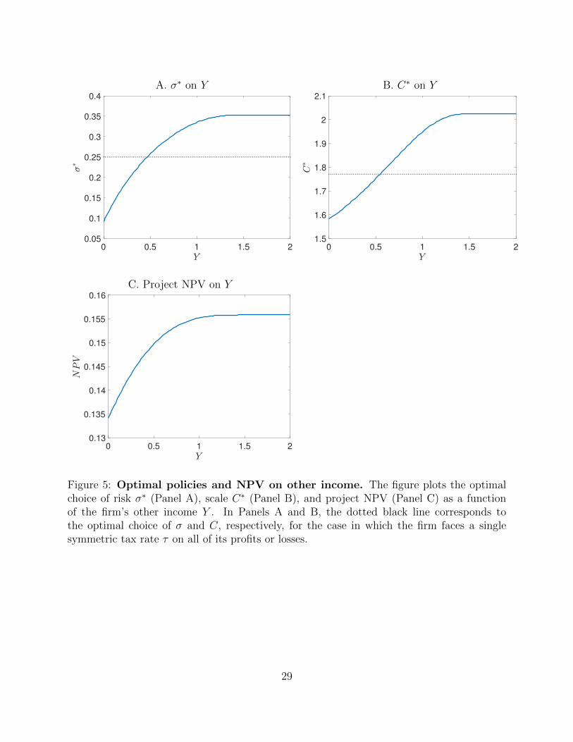
3.6 The e↵ect of the firm’s other income

With Figure 5, we show more directly the e↵ect of the firm’s other income, Y , on its

choice of policies and the NPV of the project. All parameters are set to the values reported

in Table 1. Panel A shows that the optimal riskiness of the project is increasing nonlinearly

in Y . Eventually, for a large enough value of other income (Y > C), the firm is able to

deduct all of the project losses with certainty, and an increase in Y has no further e↵ect on

the choice of �. Panels B and C similarly show that the optimal R&D expenditure and NPV

are increasing in other income and again this relationship becomes flat for a su�ciently large

amount of other income. The black dotted line in Panels A and B indicate the optimal policy

for the case where the firm faces a single constant tax rate on all of its profits or losses from

the project. For low other income, the firm chooses lower � and C than these benchmark

13

values. For higher values of Y , it chooses policies in excess of these respective benchmarks.

3.7 The e↵ect of discounted transfer pricing

In order to show the e↵ect of discounted transfer pricing, we compare the optimal policies

for scale and riskiness in a case where the firm can transfer price at a discounted price to a

case where it has to transfer the IP at the market value. In particular, we compare a case

where the discounted transfer price is set to ✓C to a case where the IP is transferred at the

market value of ✓XC↵. Figure 6 compares the optimal choice of risk and project scale, as

well as the project NPV for these two cases as a function of the US tax rate. Each row of

panels correspond to a di↵erent value of the firm’s other income Y . In each panel, the solid

blue line depicts the optimal policy or NPV for the case of discounted transfer pricing and

the dashed red line displays the case of no discount on the transfer price. Panels A, B, and

C, show that in the case where the firm has no other income (Y = 0), the choice of risk

and project scale, as well as the NPV, are slightly decreasing in the US tax rate for both

cases. However, the second row (Panels D and E) show that with a small amount of other

income Y the e↵ect of the US tax rate on optimal policies has opposite signs for the two

transfer pricing cases. When the firm is able to transfer price at a discount, the optimal scale

and riskiness are slightly increasing in the US tax rate. However, when discounted transfer

pricing is not allowed and the transfer price must be set to the market value, a higher US

tax rate results in a slightly lower choice of project riskiness and scale.

The bottom two rows of Figure 6 show that when the firm has significant other income

(Y = 1 and Y = 5), optimal riskiness and project scale increase significantly the US tax rate

when the firm is able to transfer price at a discount (p = ✓C). In contrast, when the firm

cannot transfer price at a discount, the choice of risk and project scale are una↵ected by a

change in the US tax rate. Panels I and L of the figure show that while an increase in the

US tax rate reduces the NPV in all cases, the e↵ect is significantly mitigated when a firm

can transfer price at a discount compared to the case where it cannot.

14

3.8 The choice of project risk

We assume that the firm can jointly choose the project’s scale C as well as its riskiness

�. To understand how these two choices interact, we consider an alternative case of the

model where the riskiness � is fixed and the firm can only choose the choice of project scale

C. For the case of fixed riskiness, we set � to �, the value that maximizes the expected

value of X, given by Equation (5), while all other parameters are kept at their respective

values reported in Table 1. The left column of Figure 7 plots the optimal choice of � in the

benchmark model as a function of the US tax rate for four di↵erent values of other income

Y . In each panel, the black dotted line shows the value of � for comparison. With no other

income (Y = 0), Panel A shows that the optimal choice of risk is below and decreasing

in the US tax rate. However, as the other income becomes larger, the optimal riskiness is

higher than � and increasing in the US tax rate.

The center column of Figure 7 compares the optimal choice of project scale C for the

case where the firm jointly chooses the project risk (solid blue line) to the case where the

project risk is fixed at � (dashed red line). Moving down this middle column, we see that the

firm’s other income has an important e↵ect on the relationship between the optimal scale in

these two cases. In Panel B, with no other income, the firm would like to choose a value of

� less than �. When it is unable to do so, it invests less in the project relative to the case

where it is free to choose the risk. As the US tax rate increases, the project scale declines

significantly for the fixed risk case, whereas it is roughly unchanged when the riskiness can

be jointly chosen. Panel J of the figure shows that with su�ciently large other income, there

is a complementarity in the project scale and riskiness as functions of the US tax rate. As the

US tax rate increases, the optimal project scale increases at a higher rate when the project

risk can be jointly chosen than in the case of fixed project risk.

15

4 Data

4.1 Data description and sample selection

We construct our sample from the Compustat North America Fundamentals Annual

data set. Into these data we merge the Compustat Historical Segments data set. The 1997

implementation of FAS 131 changed how publicly listed US firms reported their foreign

business segments (Albertus, Bird, Karolyi, and Ruchti (2018)). Specifically, firms began

reporting discontinuously more geographic segments starting in 1998. As a result, our sample

begins in 1998. It ends in 2015, the last year comprehensive segment data were available at

the time of writing.

We drop from the sample firms in the financial (NAICS 52-53), real estate (NAICS 53-

54), and public administration (NAICS 92-99) industries, as they may be subject to unique

regulatory regimes. In some cases, firmss’ reported segment data correspond to regions, not

countries. Since we wish to measure firms’ exposure to foreign tax rates at the country-year

level, we drop these regional segments. The result is a firm-country-year level panel, where

each segment provides the sales by the firm in a specific country.

Into this panel we merge country-year level corporate income tax rates. To obtain as

comprehensive a set of corporate income tax rates as possible, we combine data from several

sources, including KPMG’s Corporate and Indirect Tax Rate Surveys, the University of

Michigan’s World Tax Database, and the Tax Foundation. When combined, these sources

o↵er nearly complete coverage over the sample period.

On this data we impose two restrictions. First, since the tax convexity at the center of

this paper can only emerge when a firm has foreign exposure, we require that at least 10% of

a firm’s consolidated sales are reported outside the US. Second, to ensure that the firm can

use the deductions associated with undertaking risky projects in the US, we require firms

have positive net income. This results in a sample of 10,639 firm-year observations.

16

4.2 Variable construction

The key variables in the empirical analysis are the measure of risk taking and the de-

gree of the tax convexity faced by the firm. Their construction is described here. For a

comprehensive set of variable definitions, see Appendix A.

Risk, the volatility of firms’ cash flows, is the main response variable. We construct

this variable from firms’ consolidated financial data.9 We begin by calculating the ratio of

EBITDA to assets for each firm-year. Then we calculate the standard deviation of this quan-

tity for the current and three following years. If the ratio of EBITDA to assets nonmissing

for fewer than three of these years, we set Risk to be missing.

TaxRate, each firm’s weighted average tax rate, is the key predictor variable. To con-

struct this variable, we first calculate each firm’s US sales as the di↵erence between its con-

solidated sales and the sum of its sales across its foreign segments. We then obtain the firm’s

average statutory tax rate by weighting the tax rate for each country in which it has sales by

the fraction of the firm’s consolidated sales in that country. We use statutory tax rates to

mitigate endogeneity concerns, following Dharmapala (2014).10 Hence if SalesFraci,c,t is the

fraction of firm i’s consolidated sales in country c in year t and TaxRatec,t is the country’s

tax rate, then

TaxRatei,t =X

c

SalesFraci,c,t ⇥ TaxRatec,t. (16)

Conceptually, relative to the model, TaxRate combines both the di↵erence in the US

and foreign tax rates (⌧US � ⌧F ) and the fraction of the firm’s operations that are abroad

(✓). Over the sample period, the US tax rate was constant at 35%. As a result, variation in

the di↵erence between the US and foreign tax rates is determined by variation in the foreign

tax rate.9The construction follows John, Litov, and Yeung (2008).

10A possible alternative would be firms’ e↵ective tax rates. These are directly determined by firm policy

however, and may thereby exacerbate potential endogeneity problems.

17

4.3 Descriptive statistics

Table 2 display descriptive statistics. Each variable is winsorized at the 1% and 99%

thresholds of its empirical distribution to mitigate the influence of outliers. For financial

variables, we convert nominal values to 2012 values using the GDP deflator.

The mean and standard deviation of the primary response variable, Risk, are 0.069 and

0.124. The corrsponding values for the TaxRate are 0.314 and 0.035. Sample firms have

substantial foreign exposure. On average, they generate roughly 48% of their sales abroad.

Alternatively, firms have segments in 2.3 foreign countries, on average.

5 Empirical evidence

5.1 Risk taking and taxes analysis

5.1.1 Regression specification

We begin by looking at the association between the convexity in a firm’s tax rate, as

proxied by TaxRate and its cash flow volatility, as proxied by Risk. Specifically, we estimate

the following regression specification with ordinary least squares, where i and t index firms

and years.

Riski,t = � ⇥ TaxRatei,t + �0Xi,t + ↵k + ✏i,t (17)

We are parsimonious in our use of controls, indicated by Xi,t, to avoid introducing en-

dogeneity that may bias the estimate of �. In particular, we control for firm Size and Age.

In section 5.1.3, we show our results are robust to measuring firm size with either sales (our

baseline) or assets.

We also include industry fixed e↵ects, represented by ↵k, to address potential selection

concerns. For example, technology firms may tend to have both relatively risky cash flows

and proportionally larger revenues in low tax foreign jurisdictions such as Ireland. Not ac-

counting for this variation would result in a biased point estimate associated with TaxRate.11

11Indeed, the bias postulated here would go in the same direction as the economic e↵ect we hypothesize.

18

Specifically, we used fixed e↵ects corresponding to two-digit NAICS codes.

Throughout the paper, we cluster standard errors by firm.

5.1.2 Results

Table 6 contains estimates of the association between taxes and risk taking. In column

one we omit controls and fixed e↵ects. The correlation between TaxRate and Risk is negative

and statistically significant. The e↵ect is modest in economic terms, with a one standard

deviation (3.5 percentage point) lower tax rate associated with a roughly 1/13th standard

deviation (93 basis point) increase in Risk.

In column two we add controls for firm size and age. The point estimate on TaxRate

falls in magnitude while remaining statistically significant. This is driven by the negative

correlation between Risk and Size and the positive correlation between Size and TaxRate,

as indicated in Table 3.

In column three we again omit the controls but now add industry fixed e↵ects. The

coe�cient on TaxRate is between its values in columns one and two and remains statistically

significant.

Finally, in column four, we include both the controls and the fixed e↵ects. The point

estimate on TaxRate falls somewhat in magnitude to -0.124, although it remains statistically

significant. We refer to the estimates in this column as our baseline tax-risk taking estimates.

5.1.3 Robustness checks

Next, in Table 7, we turn to the robustness of the baseline taxes-risk taking result. We

begin, in column one, by modifying our calculation of Risk. The modification follows one

of the alternative measures described in John et al. (2008). Specifically, we first calculate

the average ratio of EBITDA to assets by year. We then subtract this value from the ratio

of EBITDA to assets at the firm-year level before calculating each firm’s adjusted cash flow

volatility. Arguably, this additional adjustment better isolates firms risk-taking choices from

broader economic fluctuations. The resulting point estimate corresponding to TaxRate is

19

marginally higher than the baseline estimate and remains statistically significant.

The calculations of both the key variables, Risk and TaxRate, incorporate ratios with

denominators that could take zero values. Hence a natural concern is that our results are

driven by outliers and are therefore not representative of the typical firm. It is for this reason

that we winsorize each variable at the 0.5% and 99.5% thresholds of its empirical distribution.

In column two, we confirm that these thresholds are adequate. In particular, we winsorize

each variable at the 5% and 95% thresholds and re-estimate the baseline specification. Again,

the coe�cient on TaxRate is similar in magnitude to the baseline and remains statistically

significant.

In the baseline specification, we use the natural logarithm of one plus firm sales as a

measure of firm size. We take this approach because assets appears in our calculation of

Risk. A concern may be that including the same variable on both sides of equality in a

regression specification may result in biased estimates. Nevertheless, in column three, we

use the natural logarithm of one plus assets to measure firm size. The point estimate on

TaxRate is slightly higher and again is statistically significant. If using assets to measure

size biases the estimates, its e↵ect is small.

5.2 Major tax changes

Thus far, we have presented evidence that taxes and risk taking are negatively correlated.

The strength of the above analysis is that it relies on all the variation in TaxRate – both

a firm’s exposure to foreign tax rates and changes in the tax rates themselves – that we

hypothesize should influence corporate risk taking. A drawback of this approach, however,

is that it is di�cult to ascertain whether firms’ choices of Risk are caused by variation

in TaxRate. That is, there is no clear way to evaluate whether variation in TaxRate is

plausibly exogenous.

To make some headway on this dimension, we shift our focus to instances when firms

are exposed to major tax cuts, following Giroud and Rauh (2015) and Akcigit, Grigsby,

20

Nicholas, and Stantcheva (2018).12 We define a major tax cut as an instance when a country

reduces its tax rate by at least 10 percentage points and a sample firm has at least 10% of

its consolidated sales in that country. Table 5 lists the countries, years, and magnitudes of

these changes. We then define MajorTaxCut as an indicator variable that equals one once

a firm is subject to such a tax cut. If a firm is subject to more than one major tax cut, we

omit observations for that firm in the year the second major tax cut occurs and thereafter.

With this new predictor variable, we estimate the following equation using ordinary least

squares.

Riski,t = � ⇥MajorTaxCuti,t + �0Xi,t + ↵k + ✏i,t (18)

As in equation 17, i and t index firms and years, Xi,t represents controls for Size and Age, and

↵k represents industry fixed e↵ects. The results are in Table 8. We indeed find that major

tax cuts are associated with increases in risk taking. Because MajorTaxCut is an indicator

variable, the sign is arguably more easily interpreted than the magnitude. Nevertheless, a

firm exposed to a major tax cut increases Risk by 1.1%. Recall the mean for this variable

is 6.9%.

Next we turn to the dynamics of firms’ reponses to MajorTaxCut.

Riski,t = �1 ⇥ MTCi,t�2 + �2 ⇥ MTC

i,t�1 + �3 ⇥ MTCi,t

+ �4 ⇥ MTCi+1,t + �5 ⇥ MTC

i+2+,t + �0Xi,t + ↵k + ✏i,t (19)

This specification mirrors equation 18, except MajorTaxCuti,t has been disaggregated over

time. Specifically, MTCi,t is an indicator variable that equals one in the year a tax major cut

occurs. MTCi,t�2 ,

MTCi,t�1 ,

MTCi,t+1 are defined similarly. MTC

i,t+2+ is MajorTaxCuti,t lagged twice.

We find that �1 and �2 are insignificant, consistent with the notion firms do not anticipate

12Our focus on tax cuts instead of tax changes more generally is due to the fact that there were no major

tax increases over the sample period.

21

major tax cuts. This, in turn, supports the interpretation that MajorTaxCut is exogenous

with respect to Risk.

In contrast, we find that �3, �4, and �5 are positive and statistically significant. Firms

appear to adjust their risk-taking promptly in response to changes in the convexity of their

tax schedule. Moreover, the response does not appear to substantially increase or decrease

in subsequent years. The magnitudes of �3, �4, and �5 are near that for the point estimate

associated with MajorTaxCut. These results suggest that changes in the convexity of a

firm’s tax schedule cause the firm to change the riskiness of the projects it undertakes.

6 Conclusion

This paper studies the role of transfer pricing in corporate risk taking. We use a model to

show that the di↵erential tax rates for profits in di↵erent countries combined with transfer

pricing strategies can generate an asymmetry in the after-tax gains and losses of projects

that produce intangible capital. This asymmetry can generate convexity in the payo↵s to

these projects. As a result, US multinationals face the incentive to undertake riskier and

larger scale projects.

We construct a panel of US firms with foreign operations for the period 1998–2015 to

test our predictions. Consistent with the model, we find that the tax convexity is positively

associated with risk taking. This finding is robust to potential selection concerns and holds

when we rely on major foreign tax changes as a source of variation in the tax convexity.

Dynamic results indicate these changes are unanticipated by firms, mitigating the concern

that our estimates are subject to endogeneity bias. In sum, our results suggest that the

di↵erence in tax rates US multinationals encounter domestically and abroad, in combination

with their ability to transfer price intangible capital out of the US, can influence their risk

taking activities.

22

References

Akcigit, Ufuk, John Grigsby, Tom Nicholas, and Stefanie Stantcheva, 2018, Taxation and

innovation in the 20th century, Technical report, National Bureau of Economic Research.

Albertus, James F., Andrew Bird, Stephen A. Karolyi, and Thomas G. Ruchti, 2018, Do

capital markets discipline? evidence from segment data .

Becker, Johannes, Niels Johannesen, and Nadine Riedel, 2018, Taxation and the allocation

of risk inside the multinational firm, Technical report, CESifo Group Munich.

Bernard, Andrew B, J Bradford Jensen, and Peter K Schott, 2006, Transfer pricing by

us-based multinational firms, Technical report, National Bureau of Economic Research.

Bureau of Economic Analysis, U.S. Department of Commerce, 2018, Worldwide Activities

of U.S. Multinational Enterprises: Revised 2015 Statistics .

Cristea, Anca D, and Daniel X Nguyen, 2016, Transfer pricing by multinational firms: New

evidence from foreign firm ownerships, American Economic Journal: Economic Policy 8,

170–202.

Davies, Ronald B, Julien Martin, Mathieu Parenti, and Farid Toubal, 2018, Knocking on tax

havens door: Multinational firms and transfer pricing, Review of Economics and Statistics

100, 120–134.

Dharmapala, Dhammika, 2014, What do we know about base erosion and profit shifting? a

review of the empirical literature, Fiscal Studies 35, 421–448.

Domar, Evsey D, and Richard A Musgrave, 1944, Proportional income taxation and risk-

taking, The Quarterly Journal of Economics 58, 388–422.

Favilukis, Jack, Ron Giammarino, and Jose Pizarro, 2016, Tax-loss carry forwards and

returns .

23

Giroud, Xavier, and Joshua Rauh, 2015, State taxation and the reallocation of business

activity: Evidence from establishment-level data, Technical report, National Bureau of

Economic Research.

Graham, John R, 2006, A review of taxes and corporate finance, Foundations and trends in

finance 1, 573–691.

Graham, John R, and Daniel A Rogers, 2002, Do firms hedge in response to tax incentives?,

The Journal of finance 57, 815–839.

Graham, John R, and Cli↵ord W Smith, 1999, Tax incentives to hedge, The Journal of

Finance 54, 2241–2262.

Green, Richard C, and Eli Talmor, 1985, The structure and incentive e↵ects of corporate

tax liabilities, The Journal of Finance 40, 1095–1114.

John, Kose, Lubomir Litov, and Bernard Yeung, 2008, Corporate governance and risk-taking,

The Journal of Finance 63, 1679–1728.

Langenmayr, Dominika, and Rebecca Lester, 2017, Taxation and corporate risk-taking, The

Accounting Review 93, 237–266.

Leland, Hayne E, 1998, Agency costs, risk management, and capital structure, The Journal

of Finance 53, 1213–1243.

Ljungqvist, Alexander, Liandong Zhang, and Luo Zuo, 2017, Sharing risk with the govern-

ment: How taxes a↵ect corporate risk taking, Journal of Accounting Research 55, 669–707.

Majd, Saman, and Stewart C Myers, 1985, Valuing the government’s tax claim on risky

corporate assets.

Nance, Deana R, Cli↵ord W Smith, and Charles W Smithson, 1993, On the determinants of

corporate hedging, The journal of Finance 48, 267–284.

24

Osswald, Benjamin, and Caren Sureth-Sloane, 2017, How does country risk a↵ect the impact

of taxes on corporate risk-taking? .

Pomerleau, Kyle, 2017, Corporate income tax rates around the world, 2017, Tax Foundation.

Fiscal Fact .

Ross, Michael P, 1996, Corporate hedging: What, why and how? .

Schiller, Alexander, 2015, Corporate taxation and the cross-section of stock returns, Tech-

nical report, Working paper.

Smith, Cli↵ord W, and Rene M Stulz, 1985, The determinants of firms’ hedging policies,

Journal of financial and quantitative analysis 20, 391–405.

25

Panel A: Y > 0 Panel B: Y = 0

(XC↵ � C)

Tax Paid

�Y (XC↵ � C)

Tax Paid

Figure 1: Taxes paid as a function of project income. The figure plots the taxes paid on

the project as a function of the pre-tax project income XC↵ � C. Panel A shows the tax liability

for the case in which the firm’s other income, Y , is positive. Panel B shows the case in which the

firm has no other taxable income (Y = 0). The red solid line corresponds to Region 1, the green

solid line to Region 2, and the blue solid line to Region 3, described in the text in Section 3.3. The

green dashed line is the tax liability if the firm had only domestic operations, or, alternatively if it

had to transfer price at the market value.

Panel A: Y > 0 Panel B: Y = 0

(XC↵ � C)

After-tax Payo↵

�Y (XC↵ � C)

After-tax Payo↵

Figure 2: Project after-tax payo↵ The figure plots the after-tax payo↵ on the project as a

function of the pre-tax project income XC↵�C. The solid red, green, and blue lines correspond to

Regions 1, 2, and 3, respectively, described in Section 3 of the text. The dashed green line indicates

the after-tax payo↵ the firm would have if it faced the ⌧US tax rate on all of its profits.

26

A.�⇤on

⌧ US

B.C

⇤on

⌧ US

C.Project

NPV

on⌧ U

S

0.1

50.2

0.2

50.3

0.3

50.4

0.4

50

0.1

0.2

0.3

0.4

0.5

Y =

0

Y =

0.2

Y =

1

Y =

5

0.1

50.2

0.2

50.3

0.3

50.4

0.4

51.4

1.6

1.82

2.2

2.4

2.6

Y =

0

Y =

0.2

Y =

1

Y =

5

0.1

50.2

0.2

50.3

0.3

50.4

0.4

50.1

1

0.1

2

0.1

3

0.1

4

0.1

5

0.1

6

0.1

7

Y =

0

Y =

0.2

Y =

1

Y =

5

D.�⇤on

⌧ FE.C

⇤on

⌧ FF.Project

NPV

on⌧ F

00.0

50.1

0.1

50.2

0.2

50.3

0

0.1

0.2

0.3

0.4

0.5

Y =

0

Y =

0.2

Y =

1

Y =

5

00.0

50.1

0.1

50.2

0.2

50.3

1.52

2.5

Y =

0

Y =

0.2

Y =

1

Y =

5

00.0

50.1

0.1

50.2

0.2

50.3

0.1

0.1

2

0.1

4

0.1

6

0.1

8

0.2

Y =

0

Y =

0.2

Y =

1

Y =

5

Figure

3:Compara

tivestatics

foroptimalpolicies

andNPV.Thefigu

replots

theop

timal

choice

ofscaleC

⇤(left

column),

risk

�⇤(centercolumn),

andproject

NPV

(right

column)as

afunctionof

theUStaxrate

⌧ US(top

row)an

dtheforeigntaxrate

⌧ F(bottom

row)forfourdi↵erentlevels

ofother

income:

Y=

{0,0.2,1,5}.

Allother

param

eters

arefixedat

theirvaluereportedin

Tab

le1.

27

A.�⇤on

✓B.C

⇤on

✓C.Project

NPV

on✓

0.1

0.2

0.3

0.4

0.5

0.6

0.7

0

0.1

0.2

0.3

0.4

0.5

Y =

0

Y =

0.2

Y =

1

Y =

5

0.1

0.2

0.3

0.4

0.5

0.6

0.7

1.52

2.5

Y =

0

Y =

0.2

Y =

1

Y =

5

0.1

0.2

0.3

0.4

0.5

0.6

0.7

0.1

0.1

2

0.1

4

0.1

6

0.1

8

0.2

Y =

0

Y =

0.2

Y =

1

Y =

5

D.�⇤on

↵E.C

⇤on

↵F.Project

NPV

on↵

0.7

0.7

50.8

0.8

50.9

0.0

5

0.1

0.1

5

0.2

0.2

5

0.3

0.3

5

0.4

Y =

0

Y =

0.2

Y =

1

Y =

10

0.7

0.7

50

.80

.85

0.9

01234567

Y =

0

Y =

0.2

Y =

1

Y =

10

0.7

0.7

50.8

0.8

50.9

0.1

0.1

5

0.2

0.2

5

0.3

Y =

0

Y =

0.2

Y =

1

Y =

10

Figure

4:Compara

tivestatics

foroptimalpolicies

andNPV.Thefigu

replots

theop

timal

choice

ofscaleC

⇤(left

column),risk

�⇤(centercolumn),an

dproject

NPV

(right

column)as

afunctionof

thefraction

offoreignincome✓(top

row)an

dthereturnsto

scaleparam

eter

↵(bottom

row)forfourdi↵erentlevelsof

other

incomeY.Allother

param

eters

arefixedat

theirvaluereportedin

Tab

le1.

28

A. �⇤ on Y B. C⇤ on Y

0 0.5 1 1.5 20.05

0.1

0.15

0.2

0.25

0.3

0.35

0.4

0 0.5 1 1.5 21.5

1.6

1.7

1.8

1.9

2

2.1

C. Project NPV on Y

0 0.5 1 1.5 20.13

0.135

0.14

0.145

0.15

0.155

0.16

Figure 5: Optimal policies and NPV on other income. The figure plots the optimalchoice of risk �⇤ (Panel A), scale C⇤ (Panel B), and project NPV (Panel C) as a functionof the firm’s other income Y . In Panels A and B, the dotted black line corresponds tothe optimal choice of � and C, respectively, for the case in which the firm faces a singlesymmetric tax rate ⌧ on all of its profits or losses.

29

A. �⇤ on ⌧US, Y = 0 B. C⇤ on ⌧US, Y = 0 C. NPV on ⌧US, Y = 0

0.15 0.2 0.25 0.3 0.35 0.4 0.45

0.1

0.2

0.3

0.4

0.5

0.6

0.15 0.2 0.25 0.3 0.35 0.4 0.451.57

1.58

1.59

1.6

1.61

1.62

0.15 0.2 0.25 0.3 0.35 0.4 0.450.09

0.1

0.11

0.12

0.13

0.14

0.15

0.16

D. �⇤ on ⌧US, Y = 0.5 E. C⇤ on ⌧US, Y = 0.5 F. NPV on ⌧US, Y = 0.5

0.15 0.2 0.25 0.3 0.35 0.4 0.45

0.1

0.2

0.3

0.4

0.5

0.6

0.15 0.2 0.25 0.3 0.35 0.4 0.451.66

1.68

1.7

1.72

1.74

1.76

0.15 0.2 0.25 0.3 0.35 0.4 0.450.08

0.1

0.12

0.14

0.16

0.18

G. �⇤ on ⌧US, Y = 1 H. C⇤ on ⌧US, Y = 1 I. NPV on ⌧US, Y = 1

0.15 0.2 0.25 0.3 0.35 0.4 0.45

0.1

0.2

0.3

0.4

0.5

0.6

0.15 0.2 0.25 0.3 0.35 0.4 0.451.75

1.8

1.85

1.9

1.95

2

2.05

0.15 0.2 0.25 0.3 0.35 0.4 0.450.08

0.1

0.12

0.14

0.16

0.18

J. �⇤ on ⌧US, Y = 5 K. C⇤ on ⌧US, Y = 5 L. NPV on ⌧US, Y = 5

0.15 0.2 0.25 0.3 0.35 0.4 0.45

0.1

0.2

0.3

0.4

0.5

0.6

0.15 0.2 0.25 0.3 0.35 0.4 0.451.6

1.8

2

2.2

2.4

2.6

0.15 0.2 0.25 0.3 0.35 0.4 0.450.08

0.1

0.12

0.14

0.16

0.18

Figure 6: The E↵ect of Discounted Transfer Pricing. This figure plots the optimal choice

of risk �⇤(left column), optimal choice of R&D C⇤

(center column), and the project NPV (right

column) as a function of the US tax rate. Each row corresponds to a di↵erent value of the firm’s

other income Y = {0, 0.5, 1, 5}. In each panel, the solid blue line shows the policy when the firm

can transfer its intangible capital at a discounted price of ✓C. The red dashed line shows the policy

choice if the firm were not allowed to transfer price at a discount and instead had to transfer the

intangible capital at a price equal to its market value, ✓XC↵.

30

A. �⇤ on ⌧US, Y = 0 B. C⇤ on ⌧US, Y = 0 C. NPV on ⌧US, Y = 0

0.15 0.2 0.25 0.3 0.35 0.4 0.45

0.1

0.2

0.3

0.4

0.5

0.6

0.15 0.2 0.25 0.3 0.35 0.4 0.451.1

1.2

1.3

1.4

1.5

1.6

1.7

0.15 0.2 0.25 0.3 0.35 0.4 0.450.09

0.1

0.11

0.12

0.13

0.14

0.15

0.16

C. �⇤ on ⌧US, Y = 0.5 D. C⇤ on ⌧US, Y = 0.5 E. NPV on ⌧US, Y = 0.5

0.15 0.2 0.25 0.3 0.35 0.4 0.45

0.1

0.2

0.3

0.4

0.5

0.6

0.15 0.2 0.25 0.3 0.35 0.4 0.451.7

1.72

1.74

1.76

1.78

1.8

1.82

0.15 0.2 0.25 0.3 0.35 0.4 0.450.135

0.14

0.145

0.15

0.155

0.16

0.165

0.17

F. �⇤ on ⌧US, Y = 1 G. C⇤ on ⌧US, Y = 1 H. NPV on ⌧US, Y = 1

0.15 0.2 0.25 0.3 0.35 0.4 0.45

0.1

0.2

0.3

0.4

0.5

0.6

0.15 0.2 0.25 0.3 0.35 0.4 0.451.7

1.8

1.9

2

2.1

2.2

0.15 0.2 0.25 0.3 0.35 0.4 0.450.14

0.145

0.15

0.155

0.16

0.165

0.17

I. �⇤ on ⌧US, Y = 5 J. C⇤ on ⌧US, Y = 5 K. NPV on ⌧US, Y = 5

0.15 0.2 0.25 0.3 0.35 0.4 0.45

0.1

0.2

0.3

0.4

0.5

0.6

0.15 0.2 0.25 0.3 0.35 0.4 0.451.6

1.8

2

2.2

2.4

2.6

0.15 0.2 0.25 0.3 0.35 0.4 0.450.14

0.145

0.15

0.155

0.16

0.165

0.17

Figure 7: The E↵ect of Risk Choice �. The left column shows the optimal choice of project risk �⇤

(solid blue line) as a function of the US tax rate. The dotted black line shows �, the value that maximizes

the expected pre-tax payo↵. (See Section 3 for further discussion). The center column and right column

display the optimal R&D choice (C⇤) and project NPV as functions of the US tax rate. The solid blue line

displays the optimal choice of R&D and project NPV for the case where the firm is free to choose project

risk �. The dashed red line shows these for the case where the firm cannot choose � and instead it is fixed

at �. Each row of the figure corresponds to a di↵erent value of the firm’s other income, Y = {0, 0.5, 1, 5}.31

Table 1: Model parameter values

Parameter Value

µ 0.15�1 0.1�2 0.7↵ 0.9✓ 0.4Y 0.8⌧US 0.35⌧F 0.15

The table displays the benchmark parameter values used in the model. See Section 3 for more details. µ, �1,and �2 determine the mean of the project’s productivity as a function of the choice of risk �. Specifically,

log(X) ⇠ N (µ(�),�2) where

µ(�) = µ+ (�1 � �2�)�.

↵ is the returns to scale parameter for the project, ✓ is the fraction of the firm’s operations that are foreign,

Y is the firm’s other taxable income, ⌧US is the US corporate tax rate, and ⌧F is the foreign corporate tax

rate. Unless stated otherwise, we set the discounted transfer price to ✓C.

32

Table 2: Descriptive statistics

Obs. Mean Std. dev.

Risk 10,639 0.069 0.124TaxRate 10,639 0.314 0.035Size 10,639 6.96 2.14Age 10,639 2.48 0.98FSaleFrac 10,639 0.485 0.323SegCount 10,639 2.31 2.49

This table contains descriptive statistics for the sample. Risk measures a firm’s cash flow volatility for the

current and three future years. TaxRate is a firm’s average tax rate, as weighted by the global distribution

of its sales. Detailed definitions for both these variables are contained in section 4.2. Size is the natural

logarithm of one plus sales. Age is the natural logarithm on one plus the number of years since the firm first

appears in the data. FSaleFrac is the ratio of the firm’s foreign sales to its consolidated sales. SegCount

is the number of a firm’s foreign geographic segments. All financial variables are denominated in millions of

2012 US dollars. Each variable is winsorized at the 1% and 99% thresholds of its empirical distribution to

mitigate the influence of outliers.

Table 3: Correlation matrix

Risk TaxRate Size Age FSaleFrac SegCount

Risk 1.000TaxRate -0.063 1.000

Size -0.153 0.119 1.000Age -0.041 0.109 0.323 1.000

FSaleFrac 0.061 -0.602 -0.146 -0.337 1.000SegCount -0.002 -0.055 0.107 0.138 -0.018 1.000

This table displays the correlations between the main variables used in the analysis. Risk measures a firm’s

cash flow volatility for the current and three future years. TaxRate is a firm’s average tax rate, as weighted

by the global distribution of its sales. Detailed definitions for both these variables are contained in section

4.2. Size is the natural logarithm of one plus sales. Age is the natural logarithm on one plus the number

of years since the firm first appears in the data. FSaleFrac is the ratio of the firm’s foreign sales to its

consolidated sales. SegCount is the number of a firm’s foreign geographic segments.

33

Table 4: Foeign countries with greatest activity

Panel A: 1998

Rank Country Sales

1 Canada 64,4692 Japan 59,0333 Germany 36,7754 France 33,8765 Brazil 30,2516 China 27,1587 Venezuela 26,6568 United Kingdom 20,1699 Mexico 16,35110 South Africa 11,252

Panel B: 2015

Rank Country Sales

1 Japan 516,3032 China 399,3653 Germany 384,5154 United Kingdom 334,3095 Canada 282,2496 Brazil 252,2067 France 110,2708 Russia 103,0299 Italy 79,39410 Mexico 59,619

This table lists the 10 countries with the greatest activity at the beginning (Panel A) and end (Panel B) of

the sample period.

34

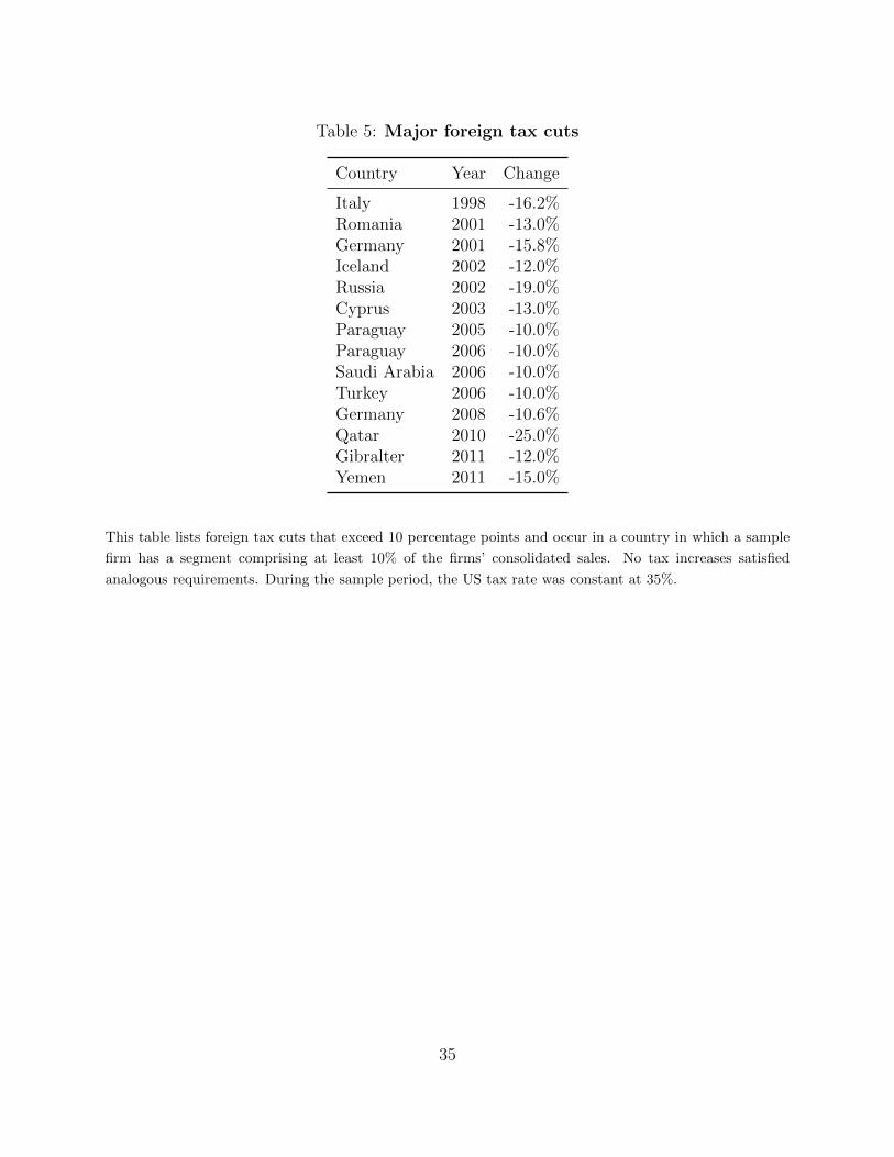
Table 5: Major foreign tax cuts

Country Year Change

Italy 1998 -16.2%Romania 2001 -13.0%Germany 2001 -15.8%Iceland 2002 -12.0%Russia 2002 -19.0%Cyprus 2003 -13.0%Paraguay 2005 -10.0%Paraguay 2006 -10.0%Saudi Arabia 2006 -10.0%Turkey 2006 -10.0%Germany 2008 -10.6%Qatar 2010 -25.0%Gibralter 2011 -12.0%Yemen 2011 -15.0%

This table lists foreign tax cuts that exceed 10 percentage points and occur in a country in which a sample

firm has a segment comprising at least 10% of the firms’ consolidated sales. No tax increases satisfied

analogous requirements. During the sample period, the US tax rate was constant at 35%.

35

Table 6: Risk taking and taxes are negatively related

Riski,t

(1) (2) (3) (4)

TaxRatei,t -0.261*** -0.171** -0.217** -0.124*(0.098) (0.084) (0.087) (0.072)

Sizei,t -0.013*** -0.013***(0.003) (0.003)

Agei,t -0.001 -0.001(0.002) (0.002)

Fixed e↵ects No No Yes Yes

Adj. R2 0.002 0.019 0.006 0.022N 10,639 10,639 10,639 10,639

This table presents results on the association between the tax convexity and risk taking. Risk measures a

firm’s cash flow volatility for the current and three future years. TaxRate is a firm’s average tax rate, as

weighted by the global distribution of its sales. Detailed definitions for both these variables are contained

in section 4.2. Size is the natural logarithm of one plus sales. Age is the natural logarithm on one plus

the number of years since the firm first appears in the data. Fixed e↵ects are by two-digit NAICS codes.

We refer to column four as the baseline estimates. Standard errors are clustered by firm. *, **, and ***

represent statistical significance at the 10%, 5%, and 1% levels, respectively.

36

Table 7: The risk taking results are robust

Riski,t

(1) (2) (3)

TaxRatei,t -0.161** -0.105** -0.149**(0.071) (0.041) (0.075)

Sizei,t -0.010*** -0.010*** -0.015***(0.003) (0.001) (0.003)

Agei,t 0.003 -0.003*** -0.000(0.002) (0.001) (0.002)

Fixed e↵ects Yes Yes Yes

Adj. R2 0.012 0.112 0.026N 10,639 10,639 10,638

This table verifies the robustness of the negative association between taxes and risk taking. In column one

we demean ratio of EBITDA to assets by year, following John, Litov, and Yeung (2008). In column two

we winsorize each variable at the 5% and 95% thresholds of its empirical distribution. In column three

we measure Size as one plus the natural logarithm of assets. Fixed e↵ects are by two-digit NAICS codes.

Standard errors are clustered by firm. *, **, and *** represent statistical significance at the 10%, 5%, and

1% levels, respectively.

37

Table 8: Major foreign tax cuts and their dynamics

Riski,t

(1) (2)

MajorTaxCuti,t 0.011**(0.005)

MTCi,t�2 -0.002

(0.004)

MTCi,t�1 0.004

(0.004)

MTCi,t 0.014***

(0.005)

MTCi,t+1 0.010*

(0.006)

MTCi,t+2+ 0.011***

(0.005)

Size -0.016*** -0.016***(0.004) (0.004)

Age -0.001 -0.001(0.004) (0.004)

Fixed e↵ects Yes YesAdj. R2 0.018 0.017Observations 9,292 9,292

This table examines the e↵ects on risk taking of major foreign tax cuts. Risk measures a firm’s cash flow

volatility for the current and three future years; a detailed definition for both this variable is contained

in section 4.2. MajorTaxCuti,t is an indicator variable that equals one once a tax cut that exceeds 10

percentage points occurs in a country in which a sample firm has a segment comprising at least 10% of the

firms’ consolidated sales.MTCi,t is an indicator variable that equals one in the year a tax major cut occurs.

MTCi,t�2 ,

MTCi,t�1 ,

MTCi,t+1 are defined similarly.

MTCi,t+2+ is MajorTaxCut lagged twice. Size is the natural

logarithm of one plus sales. Age is the natural logarithm on one plus the number of years since the firm first

appears in the data. Fixed e↵ects are by two-digit NAICS codes. Standard errors are clustered by firm. *,

**, and *** represent statistical significance at the 10%, 5%, and 1% levels, respectively.

38

A Variable definitions

• Age: The natural logarithm of one plus the number of years since the firm first appearsin the data.

• FSaleFrac: The ratio of a firm’s foreign sales to its consolidated sales.

• Risk: The riskiness of firms’ cash flows. See section 4.2 for a detailed definition.

• SegCount: The number of geographic segments corresponding to foreign countries.

• Size: The natural logarithm of one plus sales.

• TaxRate: The weighted-average tax rate. See section 4.2 for a detailed definition.

39