HDR Capture and Tone Mapping - cw.fel.cvut.cz

HDR Capture and Tone Mapping

Ing. Martin Čadík, Ph.D.

[email protected]

Martin Čadík: HDR Image Capture & Tone Mapping 2

LDR vs HDR – Comparison


Luminance

– Physically:

luminous power [lm] per unit solid angle per unit area

analogous to “what we see with our eyes”

photometric analog of radiance (weighted by luminous

efficiency function)

– In color science: weighted sum of linear RGB

Y = 0.2126 R + 0.7152 G + 0.0722 B

Luma

– Weighted sum of gamma corrected (nonlinear) RGB

Y' = 0.2126 R' + 0.7152 G' + 0.0722 B'


Various Dynamic Ranges (1)

Luminance [cd/m2]

10-6 10-4 10-2 100 102 104 106 108


Various Dynamic Ranges (2)

Luminance [cd/m2]

10-6 10-4 10-2 100 102 104 106 108Contrast

1:500

1:1500

1:30


High Dynamic Range

10-6 10-4 10-2 100 102 104 106 108

HDR Image Usual (LDR) Image


Measures of Dynamic Range

Contrast ratio CR = 1 : (Ypeak/Ynoise) displays

(e.g., 1:500 )

Orders of

magnitude

M = log10(Ypeak)-log10(Ynoise) HDR imaging

(= 2.7 orders)

Exposure latitude

(f-stops)

L = log2(Ypeak)-log2(Ynoise) photography

(= 9 f-stops)

Signal to noise

ratio (SNR)

SNR = 20*log10(Apeak/Anoise) digital cameras

(= 53 [dB])


Motivation

real world is HDR!

physically-based rendering outputs

photography

digital cinema

games (explosions are

really HDR ), video [1:04]

...

hdr_in_games/lost_coast_wmv9.wmv


HDR Applications

Image-Based Lighting

– [Debevec 98]

– using HDR radiance maps to illuminate synthetic

objects

– RNL – video1, video2

suppmtl/Movies/renderingwithnaturallight.mov

sources2/skycapture.mov


HDR Applications

physically-based rendering (global illumination)

image-based rendering and modeling

HDR panoramic imaging

visualization (i.e. medical imaging)

computer vision (algorithms may perform better)

human vision simulation and psychophysics


HDR Applications

digital photography in PS– HDR first in version: 9.0 (CS2)

– 32 bits-per-channel HDR images

– Merge To HDR command

– Photoshop (PSD, PSB), Radiance (HDR), Portable

Float Map (PFM), OpenEXR, TIFF (LogLuv just

reads)


HDR Applications


HDR Pipeline


Lecture Overview

Capture of HDR images and video

– HDR sensors

– Multi-exposure techniques

– Photometric calibration

Tone Mapping of HDR images and video

– Early ideas for reducing contrast range

– Image processing – fixing problems

– Alternative approaches

– Perceptual effects in tone mapping

Summary


HDR: a normal camera can’t…

linearity of the CCD sensor

bound to 8-14bit processors

saved in an 8bit gamma corrected image

10-6 10-4 10-2 100 102 104 106 108

perc

eiv

ed

gra

y s

had

es


HDR Sensors

logarithmic response

locally auto-adaptive

hybrid sensors (linear-logarithmic)

10-6 10-4 10-2 100 102 104 106 108

perc

eiv

ed

gra

y s

had

es


Logarithmic HDR Sensor

CMOS sensor (10bit)

Transforms collected charge to

logarithmic voltage

(analog circuit)

Dynamic range at the cost of

quantization

Very high saturation level

High noise floor

Non-linear noise

Slow response at low

luminance levels

Lin-log variants of sensor

– better quantization

– lower noise floor


Locally Auto-adaptive Sensor

Individual integration time for

each pixel

16bit sensor

– collected charge (8bit)

– integration time (8bit)

Irradiance from time and charge

Complicated noise model

Fine quantization over a wide

range

Non-continuous output!

Difficult implementation


HDR Using Multiple Sensors semi-transparent mirror

/prism

– multimple sensors with different

sensitivity

or sacrifice resolution

Panoscan Mark3,

SpheronVR (scanning

panoramic cameras), HDR

video, HDR-Cam, etc.


HDR with a normal camera

Dynamic range of a typical CCD 1:1000

Exposure variation (1/60 : 1/6000) 1:100

Aperture variation (f/2.0 : f/22.0) ~1:100

Sensitivity variation (ISO 50 : 800) ~1:10

Total operational range 1:100,000,000

Dynamic range of a single capture only 1:1000.

High Dynamic Range!


Multi-exposure Technique (1)

10-6 10-4 10-2 100 102 104 106 108

targ

et

gra

y s

had

es

Luminance [cd/m2]

+ +

HDR Imagenoise level



Input– images captured with varying exposure

change exposure time, sensitivity (ISO), ND filters

same aperture

exactly the same scene

Unknowns– camera response curve (can be given as input)

– HDR image

Process– recovery of camera response curve (if not given as input)

– linearization of input images (to account for camera response)

– normalization by exposure level

– suppression of noise

– estimation of HDR image (linear combination of input images)



f/8, 1/1000s f/5.6, 1/250s f/5.6, 1/30s

f/5.6, 1/4s f/5.6, 2s f/5.6, 8s


Algorithm (1/3)

Merge to HDR

Linearize input images and

normalize by exposure time

Weighted average of images

(weights from certainty model)

Optimize Camera Response

Camera response

Refine initial guess on response

– linear eq. (Gauss-Seidel method)i

iuviuv

t

yIx

)(1

ti exposure time of image i

yiuv pixel of input image i at position uv

I camera response

xuv HDR image at position uv

w weight from certainty model

m camera output value

i

iuv

i

iuviuv

uvw

xw

x

uviiuv xtyI )(1

mEvui

uvi

m

iuvm

xtE

mI

myvuiE

,,

1

)(Card

1)(

}:),,{(

assume I is correct (initial guess)

assume xuv is correct


Algorithm (2/3)

Certainty model (for 8bit image)

– High confidence in middle output range

– Dequantization uncertainty term

– Noise level

Longer exposures are favored ti2

– Less random noise

Weights

2)( iiuviuv tyww

2

2

5.127

)5.127(4exp)( iuv

iuv

yyw

0 50 100 150 200 2500

0.2

0.4

0.6

0.8

1


Algorithm (3/3)

1. Assume initial camera response I (linear)

2. Merge input images to HDR

3. Refine camera response

4. Normalize camera response by middle value: I-1 (m)/I-1(mmed)5. Repeat 2,3,4 until objective function is acceptable

i

iiuv

i i

iuviiuv

uvtyw

t

yItyw

x2

12

)(

)()(

mEvui

uvi

m

iuvm

xtE

mI

myjiE

,,

1

)(Card

1)(

}:),{(

2

,,

1 ))()(( uvi

vui

iuviuv xtyIywO


HDR Image

– sample

sources2/MCdesk800x600.hdr


Issues with Multi-exposures

How many source images?– First expose for shadows: all output values above 128 (for 8bit

image)

– 2 f-stops spacing (factor of 4) between images

– one or two images with 1/3 f-stop increase will improve quantization in HDR image

– Last exposure: no pixel in image with maximum value

Alignment– Shoot from tripod

– Otherwise use panorama stitching techniques to align images

Ghosting– Moving objects between exposures leave “ghosts”

– Statistical method to prevent such artifacts

Practical only for images!– Multi-exposure video projects exist, but not very successful


Other Algorithms

[Debevec & Malik 1997]

– in log space

– assumptions on the camera response

monotonic

continuous

– a lot to compute for >8bit

[Mitsunaga & Nayar 1999]

– camera response approximated with a polynomial

– very fast

Both are more robust but less general

– not possible to calibrate non-standard sensors


Calibration (Response Recovery)

Camera response can be reused

– for the same camera

– for the same picture style settings (eg. contrast)

Good calibration target

– Neutral target (e.g. Gray Card)

Minimize impact of color processing in camera

– Smooth illumination

Uniform histogram of input values

– Out-of-focus

No interference with edge aliasing and sharpening


Recovered Camera Response

recovered camera response

(for each RGB channel separately)

multiple exposures

of out-of-focus

color chart

relative luminance (log10)

cam

era

outp

ut


Photometric Calibration

Converts camera output to luminance

– requires camera response,

– and a reference measurement for known exposure

settings

Applications

– predictive rendering

– simulation of human vision response to light

– common output in systems combining different

cameras


Photometric Calibration (cntd.)

acquire

target

luminance

values

camera response

measure luminance

camera output

values


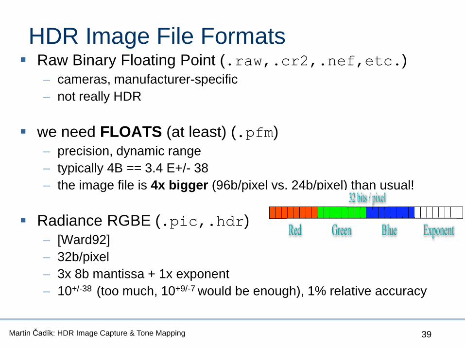
HDR Image File Formats Raw Binary Floating Point (.raw,.cr2,.nef,etc.)

– cameras, manufacturer-specific

– not really HDR

we need FLOATS (at least) (.pfm)

– precision, dynamic range

– typically 4B == 3.4 E+/- 38

– the image file is 4x bigger (96b/pixel vs. 24b/pixel) than usual!

Radiance RGBE (.pic,.hdr)

– [Ward92]

– 32b/pixel

– 3x 8b mantissa + 1x exponent

– 10+/-38 (too much, 10+9/-7 would be enough), 1% relative accuracy


HDR Image File Formats SGI LogLuv TIFF (.tif)

– [Ward 98]

– human perception based:

log encoding of luminance, 10+/-38, 0.3% relative accuracy

CIE (u, v) encoding for chroma, errors under visible threshold

– 3 variants: 24b/pixel, 30b/pixel, 32b/pixel

OpenEXR (.exr)

– Industrial Light and Magic [2003]

– 16b float (Half data type)

– 48 or 96b/pixel + lossless compression

– multiresolution

– supported by graphics hardware (NVidia, ATI frame buffers)


HDR Image File Formats JPEG HDR - Subband Encoding (.jpeg) [Ward and

Simmons 04]

– Tone-mapped version

+ Ratio image (subband – metadata JFIF)

– Ratio Image:

– allows lossy compression

– naive software = tone mapped version, specialized software =

HDREncoding pipeline Alternate decoding paths


HDR Video HDRV – perception-motivated [Mantiuk et al. 04]

– perceptual Luminance quantization

– 11b for Luminance + 2x 8b for chrominance

– based on MPEG-4

– no LDR (pure HDR video)

HDR MPEG [Mantiuk et al. 06]

– backward-compatible MPEG

– residual stream + standard LDR stream

– just 30% data flow increase


HDR Display Systems

[Seetzen et al.]– LCD panel + projector

– LCD panel + LED panel

– applications:

HDR image viewer

interactive photorealistic

rendering

volume rendering

medical image viewer


HDR Display Systems ordinary LCD

– 300:1 to 1000:1

– black=0.1 to 1 cd/m2

– peak=300 to 500 cd/m2

[brightsidetech.com]– HDR LCD

– individually modulated LEDs (not uniform backlight)

– 200 000:1

– black=0 cd/m2

– peak=4000 cd/m2

– HDR from LDR

hdr_in_games/lotr.wmv


Lecture Overview

Capture of HDR images and video

– HDR sensors

– Multi-exposure techniques

– Photometric calibration

Tone Mapping of HDR images and video

– Early ideas for reducing contrast range

– Image processing – fixing problems

– Alternative approaches

– Perceptual effects in tone mapping

Summary


HDR Tone Mapping

Many objectives of tone mapping

– nice looking images

– perceptual brightness match

– good detail visibility

– equivalent object detection performance

– really application dependent…

Luminance [cd/m2]

10-6 10-4 10-2 100 102 104 106 108


Aesthetical Cognitive Perceptual

[Čadík et al. 06]

Tone Mapping Goals

Martin Čadík: HDR Image Capture & Tone Mapping 48http://cadik.posvete.cz/tmo/

(Over)abundance of Methods


Perceptual: General Principle

[Tumblin and Rushmeier 1993]


General Ideas

Luminance as an input– absolute luminance

– relative luminance (luminance factor)

Transfer function– maps luminance to a certain pixel intensity

– may be the same for all pixels (global operators)

– may depend on spatially local neighbors (local operators)

– dynamic range is reduced to a specified range

Pixel intensity as output– often requires gamma correction

Colors– most algorithms work on luminance

use RGB to Yxy color space transform

inverse transform using tone mapped luminance

– otherwise each RGB channel processed independently


General Problems

Constraint observation conditions

– limited contrast

– quantization

– different ambient illumination

– different luminance levels

– adaptation level often incorrect for the scene

– narrow field of view

Appearance may not always be matched


Transfer Functions

Linear mapping (naïve approach)

– like taking an usual digital photo

Log function

Sigmoid responses

– simulate our photoreceptors

– simulate response of photographic film

Histogram equalization

– standard image processing

– requires detection threshold limit to prevent

contouring


Adapting Luminance

Maps luminance on a scale of gray

Task is to match gray levels

– average luminance in the scene is perceived as a gray shade of

medium brightness

– such luminance is mapped on medium brightness of a display

– the rest is mapped proportionally

Practically adjusts brightness

– like using gray card or auto-exposure in photography

– goal of adaptation processes in human vision

Adapting luminance exists in many TM algorithms

N

YYA

)log(exp


Logarithmic Tone Mapping

Logarithm is a crude

approximation of

brightness

Change of base for varied

contrast mapping in bright

and dark areas

– log10 maps better for bright

areas

– log2 maps better for dark

areas

Mapping parameter bias

in range 0.1:1

2log 10log

AY

YY '

)1)'max(log

1'log

10

)(

max

Y

YLL

Ybase

bias

Y

YYbase

5.0log

)'max(

'82)'(

[Drago et al. 03]


Sigmoid Response

Model of photoreceptor

max)(

LYfY

YL

m

A

logarithmic mapping sigmoid mapping

Brightness parameter f

Contrast parameter m

Adapting luminance YA

– average in an image

– measured pixel (equal to Y)

0

0,2

0,4

0,6

0,8

1

-5 -2,5 0 2,5 5log L

R

0,2

0,1

1


Histogram Equalization (1)

Adapts transfer function to distribution of luminance in

the image

Algorithm:

– compute histogram

– compute transfer function (cumulative distribution)

– limit slope of transfer function to prevent contouring

contouring – visible difference between 1 quantization step

use threshold versus intensity function (TVI)

TVI gives visible luminance difference for adapting luminance

“Optimal” transfer function

Not efficient when large uniform areas are present in the

image


Histogram Equalization (2)

[Ward et al. 97]


Transfer Functions Compared

Interpretation– steepness of slope is contrast

– luminance for which output is ~0 and ~1 is not transferred

Usually low contrast for dark and bright areas!


Problem with Details

Strong compression of contrast puts micro-

contrasts (details) below quantization level


Introducing Local Adaptation

Eye adapts locally to observed area

1'

'

Y

YL

AY

YY '

1'

'

LY

YL

Global adaptation YA Global YA and local adaptation YL’

Gaussian blur of HDR

image, σ ~ 1deg of

visual angle.


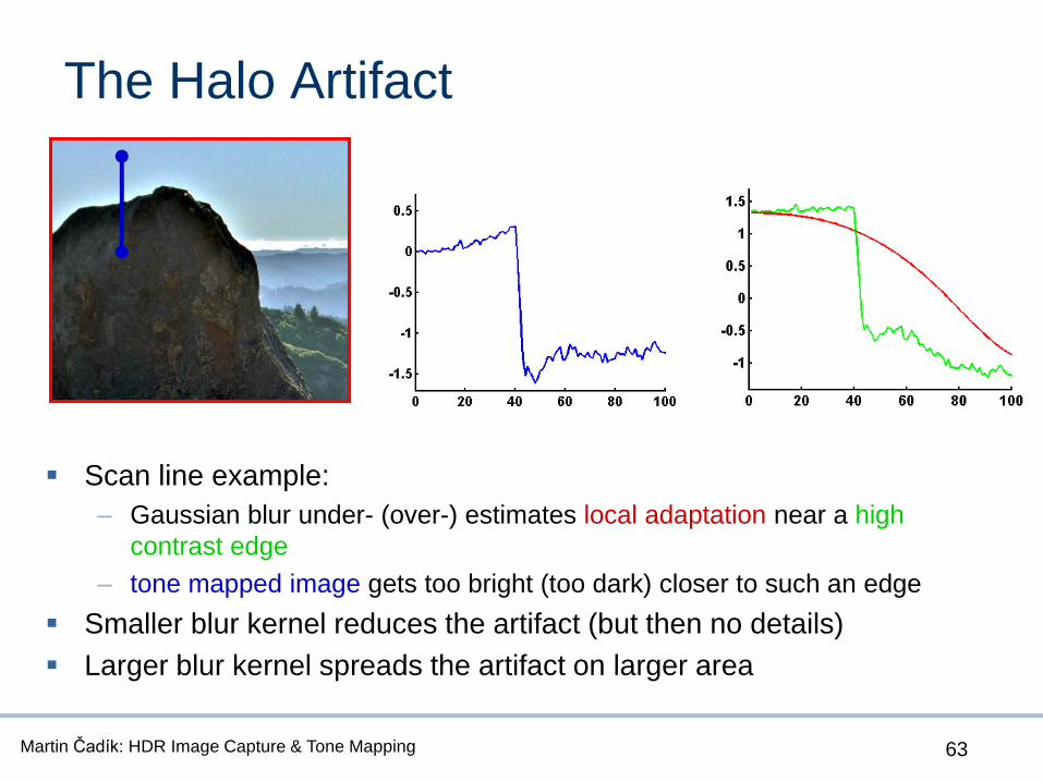
The Halo Artifact

Scan line example:

– Gaussian blur under- (over-) estimates local adaptation near a high

contrast edge

– tone mapped image gets too bright (too dark) closer to such an edge

Smaller blur kernel reduces the artifact (but then no details)

Larger blur kernel spreads the artifact on larger area


Adjusting Gaussian Blur

So called: Automatic Dodging and Burning

– for each pixel, test increasing blur size σi

– choose the largest blur which does not show halo artifact

),,(),,( 1iLiL yxYyxY[Reinhard et al. 02]


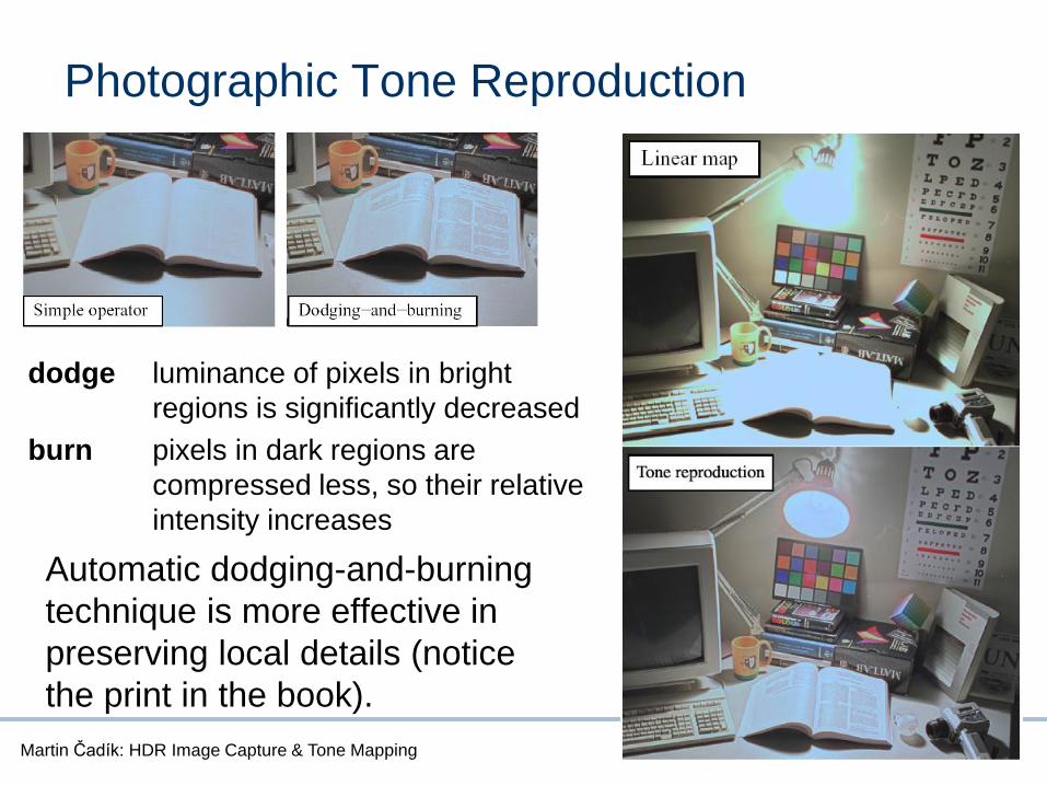
Photographic Tone Reproduction

Map luminance using Zone System

Find local adaptation for each pixel

– appropriate size of Gaussian (automatic dodging & burning)

Tone map using sigmoid function

– different blur levels from Gaussian pyramid

N

YYA

)log(exp,'

AY

YY

),,('),,(' 1iLiL yxYyxY

1),,('

),('),(

,

yxL yxY

yxYyxL

Print zones: Zone V 18% reflectance


Automatic dodging-and-burning

technique is more effective in

preserving local details (notice

the print in the book).

dodge luminance of pixels in bright

regions is significantly decreased

burn pixels in dark regions are

compressed less, so their relative

intensity increases

Photographic Tone Reproduction


Bilateral Filtering

Edge preserving Gaussian filter to prevent halo

Conceptually based on intrinsic image models:

– decoupling of illumination and reflectance layers

very simple task in CG

complicated for real-world scenes

– compress range of illumination layer

– preserve reflectance layer (details)

Bilateral filter separates:

– texture details (high frequencies, low amplitudes)

– illumination (low frequencies, high contrast edges)


Illumination Layer (1)

Identify low frequencies in the scene

– Gaussian filtering leads to halo artifacts

f - spatial kernel with large s

lost sharp edge

)(

1

pNq

q

p

p IqpfW

Js


Edge preserving filter – no halo artifacts

f - spatial kernel with large s

g - range kernel with very small r

Illumination Layer (2)

)(

1

pNq

qqp

p

p IIIgqpfW

Jrs


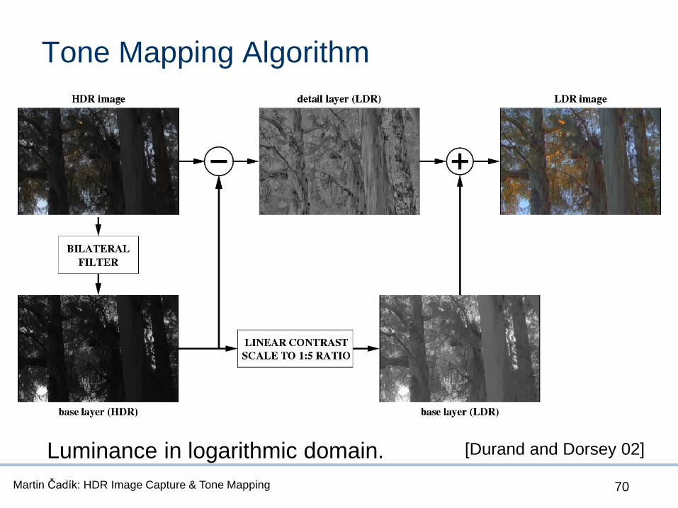
Tone Mapping Algorithm

Luminance in logarithmic domain. [Durand and Dorsey 02]


Illumination & Reflectance


Alternative Approaches to TM

Gradient domain tone mapping

– transfer function for contrasts (not luminance)

Segmentation for tone Mapping

– based on perception theory and Gestalt assumptions

– fuzzy segmentation based on illumination

– simple tone mapping within segments


1. Calculate gradients map of image

2. Calculate attenuation map

3. Attenuate gradients

4. Solve Poisson equation to recover image

Gradient Compression Algorithm

H = log L

Ld = exp I

[Fattal et al. 02]


Attenuation Map

1. Create Gaussian pyramid

2. Calculate gradients on levels

3. Calculate attenuation on levels - k

4. Propagate levels to full resolution


Transfer Function for Contrasts

Attenuate large gradients– presumably illumination

Amplify small gradients– hopefully texture details

– but also noise

1.0

9.0

small gradients large gradients


Global vs. Local Compression

Loss of overall contrast

Loss of texture details

Short execution time

Simple hardware implementation

Impression of high contrast

Good preservation of fine details

Takes time

Complicated hardware implementation


Alternative Approaches to TM

Gradient domain tone mapping

– transfer function for contrasts not luminance

– basic idea today

– contrast processing framework on the next lecture

Segmentation for Tone Mapping

– based on perception theory and Gestalt assumptions

– fuzzy segmentation based on illumination

– simple tone mapping within segments


Lightness Perception

Lightness depends strongly on the context(according to “Anchoring Theory of Lightness Perception”)

And does not depend on:

– absolute luminance

– its relation with background

(this is against contrast theories)

Fuzzy segmentation for tone mapping

– to find spatial contexts

– to tone map within such contexts

[Krawczyk et al. 06]


Estimation of Lightness

Constant lightness within certain image areas

Image copyrights: Magnum Photos.


The Theory“An Anchoring Theory of Lightness Perception”

developed by Gilchrist et al. 1999

Key concepts:

Frameworks – areas of common illumination

Anchoring – luminance → lightness mapping

∑


Fuzzy Segmentation

Perceptual organization:– semantic grouping

– good continuation

– grouping of illumination

– proximity

Probability maps define segments


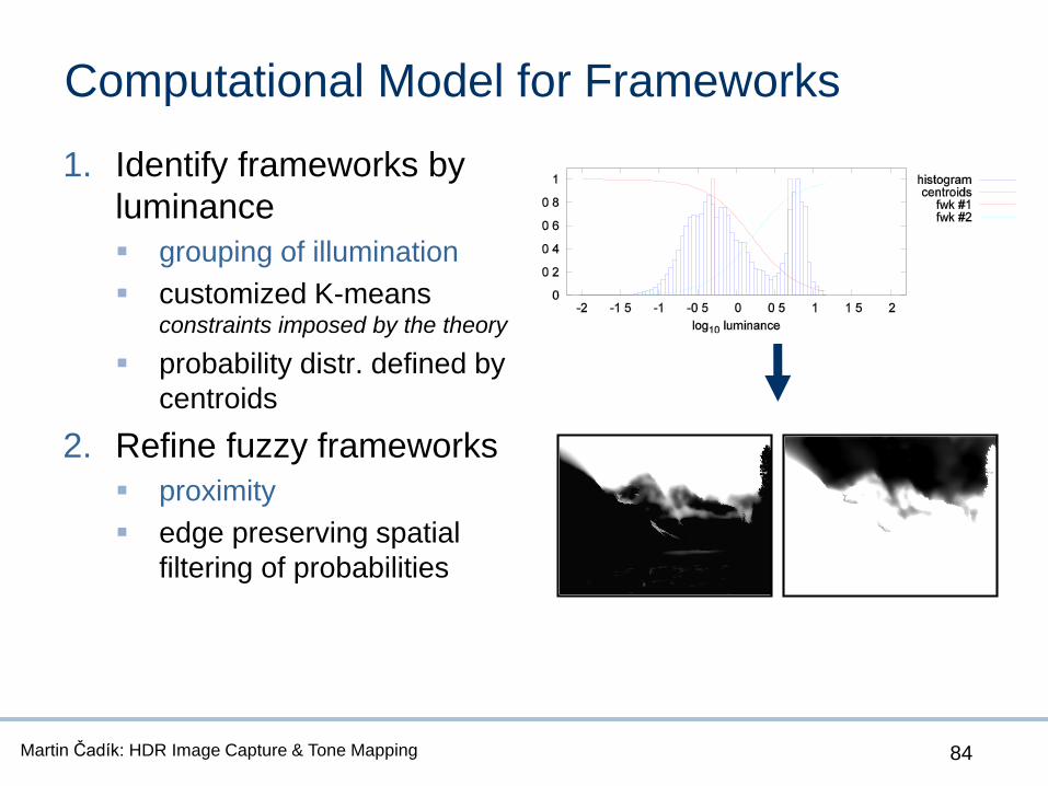
Computational Model for Frameworks

1. Identify frameworks by

luminance

grouping of illumination

customized K-meansconstraints imposed by the theory

probability distr. defined by

centroids

2. Refine fuzzy frameworks

proximity

edge preserving spatial

filtering of probabilities


Lightness in Frameworks

Anchoring to white:

– highest luminance appears

white

– highest luminance may

appear self-luminous

Our approach:

– filter framework area to

eliminate highlights

– highest luminance in

framework becomes an anchor

white

gray

black

self

luminous


Net LightnessShift original luminance Y(x,y)

– according to local lightness (framework’s local anchor Wi)

– proportionally to probabilities Pi(x,y) and framework articulation Di

– constant influence of the global framework (global anchor W0)


Testing: Advanced Lightness Estimation

Tone mapping of the Gelb illusion


Analysis of Gelb Illusion

most of tone mapping

methods

tone mapping of

illumination layer

lightness perception

modelframeworks


Perceptual Effects in TM

Simulate effects that do not appear on a screen but are typically

observed in real-world scenes

– veiling glare

– night vision

– temporal adaptation to light

Increase believability of results, because we associate such effects

with luminance conditions


Temporal Luminance Adaptation

Compensates changes in illumination

Simulated by smoothing adapting

luminance in tone mapping equation

Different speed of adaptation to light

and to darkness


Night Vision

Human Vision operates in three distinct adaptation

conditions:


Visual Acuity

Perception of spatial details is limited with decreasing

illumination level

Details can be removed using

convolution with a Gaussian kernel

Highest resolvable spatial frequency:


Veiling Luminance (Glare)

Decrease of contrast and visibility due to light scattering

in the optical system of the eye

Described by the optical transfer

function:


Fast TM on GPU

Simple transfer function is very fast

What about those advanced algorithms

– bilateral: fast approximate algorithms available

– gradient domain: GPU needs ~100ms per 1MPx

Real-time?

– automatic dodging & burning

– Gaussian pyramid can be built fast on GPU

– the pyramid can be used to add perceptual effects at

no additional cost!


HDR Video Player with

Perceptual Effects

../../MPI/Research%20Demo/HDR%20Video%20-%20Perceptual%20Effects.avi

../../MPI/Research%20Demo/HDR%20Video%20-%20Perceptual%20Effects.avi


Thank You

[email protected]

Many thanks to Karol Myszkowski and MPII Saarbrücken HDRI crowd


Papers about Calibration

Estimation-Theoretic Approach to Dynamic Range Improvement Using Multiple Exposures

– M. Robertson, S. Borman, and R. Stevenson

– In: Journal of Electronic Imaging, vol. 12(2), April 2003.

Recovering High Dynamic Range Radiance Maps from Photographs– Paul E. Debevec and Jitendra Malik

– In: SIGGRAPH 97

Radiometric Self Calibration– T. Mitsunaga and S.K. Nayar

– In: Computer Vision and Pattern Recognition (CVPR), 1999.

High Dynamic Range from Multiple Images: Which Exposures to Combine?– M.D. Grossberg and S.K. Nayar

– In: ICCV Workshop on Color and Photometric Methods in Computer Vision (CPMCV), 2003.


Papers about Tone Mapping Adaptive Logarithmic Mapping for Displaying High Contrast Scenes

– F. Drago, K. Myszkowski, T. Annen, and N. Chiba

– In: Eurographics 2003

Photographic Tone Reproduction for Digital Images– E. Reinhard, M. Stark, P. Shirley, and J. Ferwerda

– In: SIGGRAPH 2002 (ACM Transactions on Graphics)

Fast Bilateral Filtering for the Display of High-Dynamic-Range Images– F. Durand and J. Dorsey


Gradient Domain High Dynamic Range Compression– R. Fattal, D. Lischinski, and M. Werman


Dynamic Range Reduction Inspired by Photoreceptor Physiology– E. Reinhard and K. Devlin

– In IEEE Transactions on Visualization and Computer Graphics, 2005

Time-Dependent Visual Adaptation for Realistic Image Display– S.N. Pattanaik, J. Tumblin, H. Yee, and D.P. Greenberg

– In: Proceedings of ACM SIGGRAPH 2000

Lightness Perception in Tone Reproduction for High Dynamic Range Images– G. Krawczyk, K. Myszkowski, H.-P. Seidel

– In: Eurographics 2005

Perceptual Effects in Real-time Tone Mapping– G. Krawczyk, K. Myszkowski, H.-P. Seidel

– In: Spring Conference on Computer Graphics, 2005

Evaluation of HDR Tone Mapping Methods Using Essential Perceptual Attributes – M. Čadík, M. Wimmer, L. Neumann, A. Artusi

HDR Capture and Tone Mapping - cw.fel.cvut.cz

Documents

Transcript of HDR Capture and Tone Mapping - cw.fel.cvut.cz