Have out your calculator and your notes! The four C’s: Clear, Concise, Complete, Context.
64
Have out your calculator and your notes! The four C’s: Clear, Concise, Complete, Context
-
Upload
morgan-blake -
Category
Documents
-
view
221 -
download
2
Transcript of Have out your calculator and your notes! The four C’s: Clear, Concise, Complete, Context.

Have out your calculator and your notes!
The four C’s:Clear, Concise, Complete, Context

Chapter 4
Displaying Quantitative Data

Dealing With a Lot of Numbers... When looking at large sets of quantitative
data, it can be difficult to get a sense of what the numbers are telling us without summarizing the numbers in some way.
In this chapter, we will concentrate on graphical displays of quantitative data.

Percent of Population over 65 per state (1996)13.0 14.3 12.5 13.9 13.8 12.5 15.8 12.1
5.2 12.8 12.6 11.4 11.4 14.5 12.1 11.2
13.2 18.5 15.2 14.1 12.0 13.4 14.4 11.6
14.4 9.9 13.7 12.4 13.8 13.5 12.5 15.2
10.5 12.9 12.6 12.4 11.0 13.4 10.2 13.3
11.0 11.4 11.4 12.3 13.4 15.9 8.8 11.2
13.8 13.2
Put this in your calc!!! (L1)

What do these data tell us?
Make a picture Histogram Stem-and-Leaf Display Dot plot
First three things to do with data Make a picture Make a picture Make a picture

Displaying Quantitative Data
Histogram Give each graph a title Give each one of the axes a label Make as neat as possible
• Computer• Calculator• Grid paper

Displaying Quantitative Data
Histogram Divide data values into equal-width piles
(called bins) Count number of values in each bin Plot the bins on x-axis Plot the bin counts on y-axis

Example – Population Over 65
Decide on bin values Low value is 5.2 and high value is 18.5 Bins are 5.0 up to 6.0, 6.0 up to 7.0, etc. Written as 5.0 ≤ X < 6.0, 6.0 ≤ X < 7.0
Count number of values in each bin Bin 5.0 ≤ X < 6.0 has 1 value Bin 6.0 ≤ X < 7.0 has 0 values Bin 7.0 ≤ X < 8.0 has 0 values Bin 8.0 ≤ X < 9.0 has 1 value Continue counting values in each bin
“Up to but not including”

Example – Population Over 65
Plot bins on x-axis Min: 5.2 and max: 18.5 14 bins from 5.0 ≤ X < 6.0 to 18.0 ≤ X < 19.0
Plot bin counts on y-axis Bin counts are:
1, 0, 0, 1, 1, 2, 9, 13, 13, 5, 4, 0, 0, 1

Make one on your
calc!!!

Displaying Quantitative Data
Stem and Leaf Display Picture of Distribution Generally used for smaller data sets Group data like histograms Still have original values (unlike
histograms) Two columns
• Left column: Stem• Right column: Leaf

Displaying Quantitative Data
Stem and Leaf Display Leaf
• Contains the last digit of the values• Arranged in increasing order away from stem
Stem• Contains the rest of the values• Arranged in increasing order from top to bottom
**Always have a legend!**

Example – Population Over 65
Leaf = tenths digit Stem = tens and ones digits Ex. 5 | 2 Ex. 10| 2 5 Ex. 14| 1 3 4 4 5

Percent of Population over Age 65 (by state) in 1996
5 2678 89 9
10 2 511 0 0 2 2 4 4 4 4 612 0 1 1 3 4 4 5 5 5 6 6 8 913 0 2 2 3 4 4 4 5 7 8 8 8 914 1 3 4 4 515 2 2 8 9161718 5
12 | 1 = 12.1%

Same shape!
5 2678 89 9
10 2 511 0 0 2 2 4 4 4 4 612 0 1 1 3 4 4 5 5 5 6 6 8 913 0 2 2 3 4 4 4 5 7 8 8 8 914 1 3 4 4 515 2 2 8 9161718 5
52
6 7 88
99
102
511
00
22
44
44
612
01
13
44
55
56
68
913
02
23
44
45
78
88
914
13
44
515
22
89
16 17 185

Example – Frank Thomas
Career Home Runs (1990-2004)
4 7 15 18 24 28 29 32 35 38 40 40 41 42 43
0 4 71 5 82 4 8 93 2 5 84 0 0 1 2 3
1 | 8 = 18 home runs

Displaying Quantitative Data
Back-to-back Stem-and-Leaf Display Used to compare two variables Stems in center column Leafs for one variable – right side Leafs for other variable – left side Arrange leafs in increasing order,
AWAY FROM STEM!

Example – Compare Frank Thomas to Ryne Sandberg
Career Home Runs for Ryne Sandberg (1981-1997)
0 5 7 8 9 12 14 16 19 19 25 26 26 26 30 40
SandbergThomas
9 8 7 5 0 0 4 79 9 6 4 2 1 5 86 6 6 5 2 4 8 9
0 3 2 5 80 4 0 1 2 3
1 | 8 = 18 home runs

Displaying Quantitative Data
If there are a large number of observations in only a few stems, we can split stems.
Split the stems into two stems First stem is 0 – 4. Second stem is 5 – 9.
If you choose to split one stem you MUST split them all!
Example – Population Over 65
12 0 1 1 3 4 4 5 5 5 6 6 8 913 0 2 2 3 4 4 4 5 7 8 8 8 9
12 0 1 1 3 4 412 5 5 5 6 6 813 0 2 2 3 4 413 5 7 8 8 8 9 12 | 1 = 12.1%

One Variable Statistics… Population Over 65:
STAT > CALC > 1-Var Stats

Looking at Distributions
Always report 4 things when describing a distribution:
1. Shape
2. Unusual (Outliers and other notable features)
3. Center
4. Spread
SUCS (Shape, Unusual, Center, Spread)

Looking at Distributions
Shape How many humps (called modes)?
• None = uniform• One = unimodal• Two = bimodal• Three or more = multimodal

0.1 0.2 0.3 0.4
0
5
10
15
Size (carats)
Fre
qu
ency
Size of Diamonds (carats)
86 87 88 89 90 91 92 93 94 95 96
0
1
2
3
4
5
6
7
8
9
10
Octane
Fre
qu
ency
Histogram of Octane Rating

Looking at Distributions Shape
Is it symmetric?• Symmetric = roughly equal on both sides• Skewed = more values on one side
• Right = Tail stretches to large values• Left = Tail stretches to small values
Are there any outliers?• Interesting observations in data• Can impact statistical methods
86 87 88 89 90 91 92 93 94 95 96
0
1
2
3
4
5
6
7
8
9
10
OctaneF
req
uen
cy
Histogram of Octane Rating

Examples of Skewness
“Skewness to the fewness”

Looking at Distributions
Center A single number to describe the data Can calculate different numbers for center

Looking at Distributions
Spread Variation in the data values
• Range: Smallest observation to the largest observation
• May take into account any outliers• Later, spread will be a single number

SUCS (Shape, Unusual, Center, Spread)

Example – Population Over 65 Shape
Unimodal Symmetric
Unusual Two Outliers (5% and 18%)
Center: About 12% Spread: Almost all
observations are between 8% and 16%
SUCS (Shape, Unusual, Center, Spread)

Now try… (Day one)
Pg. 72 #5-12
“My father taught me that the only way you can make good at anything is to practice, and then practice some more.”
-Pete Rose

Example – Frank Thomas
• Shape– Unimodal – Skewed left– No outliers
• Center: Median = 32 home runs
• Spread: All values are between 4 and 43
0 4 71 5 82 4 8 93 2 5 84 0 0 1 2 3
1 | 8 = 18 home runs

Example – Compare Frank Thomas to Ryne Sandberg
• Sandberg’s Home Runs Shape:
– Unimodal
– Skewed right****
– No Outliers
• Center: Median = 27.5 home runs
• Spread: All values are between 0 and 40
• Both players have about the same spread (ranges are 40 and 39)
• Thomas has 50% of his home runs above 30, while Sandberg only has 6.25% above 30.
9 8 7 5 0 0 4 79 9 6 4 2 1 5 86 6 6 5 2 4 8 9
0 3 2 5 80 4 0 1 2 3
1 | 8 = 18 home runs

What Do We Know?
Histograms, Stem-and-Leaf Displays, Back-to-Back Stem-and-Leaf Displays
When describing a display, always mention: Shape: number of modes, symmetric or skewed Unusual Features (Outliers, etc. Mention them if
they exist; otherwise, say there are no outliers) Center Spread
SUCS (Shape, Unusual, Center, Spread)

What Do We Know? (cont.)
A graph is either symmetric or skewed, not both!
If a graph is skewed, be sure to specify the direction: Skewed left (negative) or skewed right
(positive)… (“Skewness to the fewness”)

Describing the Distribution
Center Median (.5 quantile, 2nd quartile, 50th percentile) Mean
Spread Range (max – min) Interquartile Range (Q3 – Q1) Standard Deviation

Median
Literally = middle number (data value) Has the same units as the data n (number of observations) is odd
Order the data from smallest to largest Median is the middle number on the list (n+1)/2 number from the smallest value
• Ex: If n=11, median is the (11+1)/2 = 6th number from the smallest value
• Ex: If n=37, median is the (37+1)/2 = 19th number from the smallest value
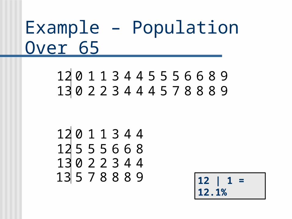
Example – Frank Thomas
Career Home Runs 4 7 15 18 24 28 29 32 35 38 40 40 41 42 43
Remember to order the values, if they aren’t already in order!
• 15 observations (15+1)/2 = 8th
observation from bottom
• Median = 32 HRs

Median
n is even Order the data from smallest to largest Median is the average of the two middle
numbers (n+1)/2 will be halfway between these two
numbers• Ex: If n=10, (10+1)/2 = 5.5, median is average
of 5th and 6th numbers from smallest value

Example – Ryne Sandberg
Career Home Runs0 5 7 8 9 12 14 16 19 19 25 26 26 26 30 40
Remember to order the values if they aren’t already in order!
• 16 observations (16 + 1)/2 = 8.5,
average of 8th and 9th observations from bottom
• Median = average of 16 and 19
• Median = 17.5 HRs

Mean
Everyday “average” that most people think of Add up all observations Divide by the number of observations Has the same units as the data
Formula n observations y1, y2, y3, …, yn are the values

Mean
y y1 y2 y3 L yn
n
yn
1
ny

Examples of mean…
Thomas’ Career Home Runs:
Sandberg’s Career Home Runs:
(4 7 15 18 ... 43)
1526.4HRs
(0 5 7 8 ... 40)
1617.625 HRs
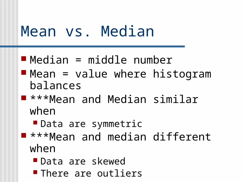
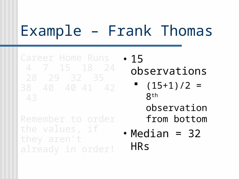
Mean vs. Median
Median = middle number Mean = value where histogram
balances ***Mean and Median similar when
Data are symmetric ***Mean and median different when
Data are skewed There are outliers

Mean vs. Median
Mean influenced by unusually high or unusually low values Example: Income in a small town of 6
people$25,000 $27,000 $29,000 $35,000 $37,000 $38,000
**The mean income is $31,830**The median income is $32,000
And then….

Mean vs. Median
Bill Gates moves to town$25,000 $27,000 $29,000
$35,000 $37,000 $38,000 $40,000,000
**The mean income is $5,741,571
**The median income is $35,000 Mean is pulled by the outlier Median is not Mean is not a good center of these data

Mean vs. Median Skewness pulls the mean in the
direction of the tail Skewed to the right = mean > median Skewed to the left = mean < median
Outliers pull the mean in their direction Large outlier = mean > median Small outlier = mean < median

Spread
Range = maximum – minimum Thomas
Min = 4, Max = 43, Range = 43 - 4 = 39 HRs Sandberg
Min = 0, Max = 40, Range = 40 - 0 = 40 HRs

Spread
Range is a very basic measure of spread It is highly affected by outliers Makes spread appear larger than reality Ex. The annual numbers of deaths from
tornadoes in the U.S. from 1990 to 2000: 53 39 39 33 69 30 25 67 130 94 40
• Range with outlier: 130 – 25 = 105 tornadoes• Range without outlier: 94 – 25 = 69 tornadoes

Spread
Interquartile Range (IQR) First Quartile (Q1)
• Larger than about 25% of the data Third Quartile (Q3)
• Larger than about 75% of the data
IQR = Q3 – Q1 Center (Middle) 50% of the values
The IQR is a single value,
NOT AN INTERVAL!

Finding Quartiles
Order the data Split into two halves at the median
When n is odd, include the median in both halves
When n is even, do not include the median in either half
Q1 = median of the lower half Q3 = median of the upper half

Example – Frank Thomas
Order the values (15 values)
4 7 15 18 24 28 29 32 35
38 40 40 41 42 43
Lower Half = 4 7 15 18 24 28 29 32 Q1 = Median of lower half = 21 HRs
Upper Half = 32 35 38 40 40 41 42 43 Q3 = Median of upper half = 40 HRs
IQR = 40 – 21 = 19 HRs

Example – Ryne Sandberg
Order the values (16 values) 0 5 7 8 9 12 14 16 19 19 25 26 26 26 30 40
Lower Half = 0 5 7 8 9 12 14 16 Q1 = Median of lower half = 8.5 HRs
Upper Half =19 19 25 26 26 26 30 40 Q3 = Median of upper half = 26 HRs
IQR = Q3 – Q1 = 26 – 8.5 = 17.5 HRs

Five Number Summary
Minimum Q1 Median Q3 Maximum
We’ll use these to make boxplots next chapter!

Examples Thomas
Min = 4 HRs Q1 = 21 HRs Median = 32 HRs Q3 = 40 HRs Max = 43 HRs
Sandberg Min = 0 HRs Q1 = 8.5 HRs Median = 17.5 HRs Q3 = 26 HRs Max = 40 HRs

Spread
Standard deviation “Average” spread from mean Most common measure of spread
• (Although it is influenced by skewness and outliers)
Denoted by letter s Make a table when calculating by hand

Standard Deviation
s (y1 y )2 (y2 y )2 K (yn y )2
n 1
y y 2n 1
1
n 1y y 2

Example – Deaths from Tornadoes
53 53-56.27 =-3.27 10.69
39 39-56.27 = -17.27 298.25
39 39-56.27 = -17.27 298.25
33 33-56.27 = -23.27 541.49
69 69-56.27 = 12.73 162.05
30 30-56.27 = -26.27 690.11
25 25-56.27 = -31.27 977.81
67 67-56.27 = 10.73 115.13
130 130-56.27 = 73.73 5436.11
94 94-56.27 = 37.73 1423.55
40 40-56.27 = -16.27 264.71
y )( yy 2)( yy
s 10.69 298.25 L 264.71
11 131.97 tornadoes
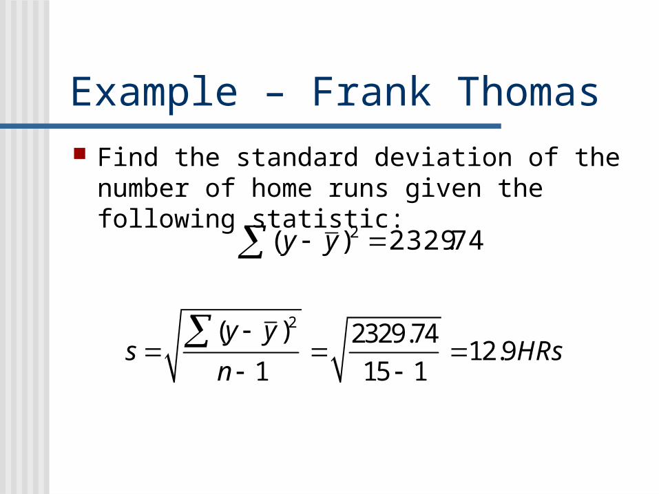
Example – Frank Thomas Find the standard deviation of the number of
home runs given the following statistic:
74.2329)( 2 yy
s (y y )2n 1
2329.74
15 112.9HRs

Properties of s
s = 0 only when all observations are equal; otherwise, s > 0
s has the same units as the data s is not resistant…
Skewness and outliers affect s, just like mean Tornado Example:
• s with outlier: 31.97 tornadoes• s without outlier: 21.70 tornadoes

Which summaries should you use? What numbers are affected by outliers?
Mean Standard deviation Range
What numbers are not affected by outliers? Median IQR
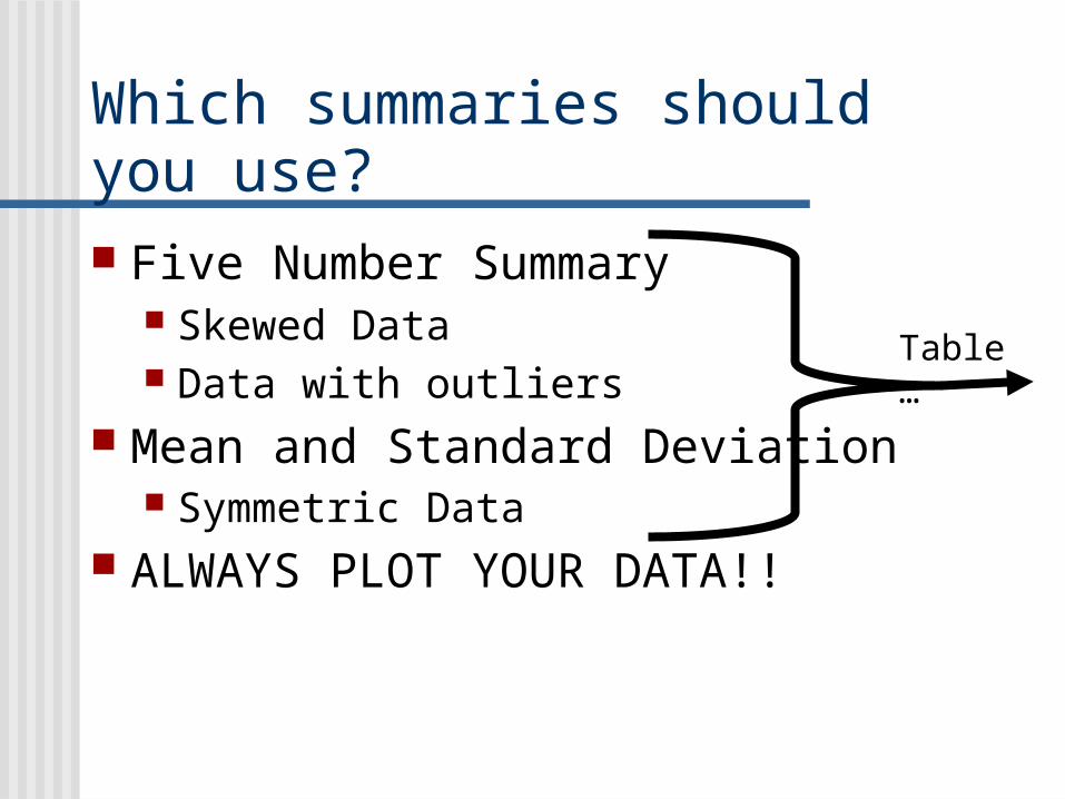
Which summaries should you use? Five Number Summary
Skewed Data Data with outliers
Mean and Standard Deviation Symmetric Data
ALWAYS PLOT YOUR DATA!!
Table…

Now try… (Day two)
Pg. 72 #13-23 odds

Now try…do… (Day three)
Pg. 72-78 #25, 29, 31,
37, 43, 45, 49