1

Have International Transportation Costs Declined?

David HummelsUniversity of Chicago

July 1999

Abstract:

While the precise causes of post-war trade growth are not well understood, declines in transportcosts top the lists of usual suspects. However, there is remarkably little systematic evidencedocumenting the decline. This paper provides a detailed accounting of the time-series pattern ofshipping costs. Direct evidence from an eclectic mix of data shows that ocean freight rates haveincreased while air freight rates have declined rapidly. Indirect evidence suggests that the cost ofoverland transport has declined relative to ocean transport. For all modes, the freight costsassociated with increased distance have declined. Data on the changing composition of trade arebroadly consistent with these changes in relative prices.

Acknowledgments: Thanks for comments go to Jim Harrigan, Alan Deardorff and seminarparticipants at the University of Chicago. Yong Kim, Julia Grebelsky and Dawn Conner providedoutstanding research assistance. This research was funded by a grant from the University of Chicago’sGraduate School of Business.

Contact Information: University of Chicago, Graduate School of Business, 1101 E. 58 ST, Chicago IL 60637. Ph:773-702-5141; Fax: 773-702-0458; email: david.hummels@gsb.uchicago.edu

2

I. Introduction

Have international transportation costs declined? Several papers by Harley (1980, 1988,

1989) and North (1958, 1968) provide evidence of substantial reductions in shipping costs from

1850-1913, a period in which world trade grew rapidly. The post-war era has also been

characterized by rapid trade growth, and while the precise causes of that growth are not well

understood, declines in transport costs top the lists of usual suspects.1 Unlike the earlier period,

however, there is remarkably little systematic evidence documenting the decline.2 This paper

provides a detailed accounting of the time-series pattern of shipping costs. In addition, it offers

insights into how changes in the nature of transportation have affected the composition of trade.

A better understanding of international integration, its causes and consequences, requires

the careful measurement of trade barriers. The level of barriers has implications for a broad

range of questions, from the welfare consequences of trade growth3, to the extent of product and

factor price equalization, the effect of trade on domestic competition, and the diffusion of

technology embodied in goods, among others. Further, relative changes in barriers of different

types may alter the composition of trade, or provide incentives to shift to other forms of

integration. For example, declines in the cost of air relative to ocean transport may greatly

facilitate trade in time-sensitive goods. Similarly, if the cost of moving goods remains high

while the cost of moving information about goods declines, firms may find direct investment

more efficient than trade for serving foreign markets.

The term “transport cost” in popular use subsumes shipping expenses but is also used

loosely as a catch-all for any number of important costs that impede trade. This paper focuses on

shipping costs rather than a broader basket of component costs for three reasons. One,

measurement must start somewhere and it is sensible to begin in obvious places. Two, changes

in shipping costs can be directly interpreted in terms of their effect on trade -- all trade

1 See Krugman (1995). Recent papers by Rose (1991), Baier and Bergstrand (1998) and Djankov, Evenett, andYeung (1998) have attempted to attribute trade growth to changes in tariffs, transport costs as measured by IMFcif/fob ratios, and other causal factors.2 An exception is Lundgren (1996), who relies on a very small number of goods and routes to conclude that theconstant dollar price of shipping a ton of bulk commodities fell substantially between 1950 and 1993. However, asshown in section II of the current paper, the ad-valorem barrier posed by shipping has not fallen for bulkcommodities, and a considerably broader set of data reveals a general pattern of shipping cost increases.3 Small reductions in trade barriers yield large trade volume increases (and little additional gain from trade) ifforeign and domestic goods are sufficiently close substitutes in production or consumption. See Yi (1999) andHummels, Ishii and Yi (1999) for more on this point.

3

necessarily requires shipping and the ad-valorem equivalent of the barrier is simple to calculate.

In contrast, we know that the cost of moving information has declined orders of magnitude but

not how this relates to trade. (What fraction of costs do international telephone calls represent

for the average exporter?) Three, papers that have directly investigated the relative importance

of shipping versus tariff barriers in the cross-section have consistently identified shipping costs

as the more important barrier.4 This evidence, which covers many countries and several decades,

suggests that a careful accounting of time-series change in trade barriers as a whole must include

a careful accounting of time-series change in shipping costs.

Unfortunately, there is no single source of data that provides a definitive picture of the

costs of transport. One source with great breadth of coverage, matched partner reports of trade

flows available from the IMF, has been used by a number of authors use to assess transportation

costs across countries and over time.5 In principle, exporting countries report trade flows

exclusive of freight and insurance (fob), and importing countries report flows inclusive of freight

and insurance (cif). Comparing the valuation of the same aggregate flow reported by both the

importer and exporter yields a difference equal to transport costs. The time series derived from

IMF sources accords well with conventional wisdom -- transportation costs have declined

steadily while trade has grown (see Table A1). However these data are subject to two serious

problems. First, as an appendix details, the IMF data are of extremely low quality, and rely on

extensive imputation. Second, as aggregate data they are subject to compositional effects that

mask the true time series in transport costs. Shifts in the types of goods traded, or the sets of

partners with whom a country trades, will affect measured costs even if the unit cost of shipping

remains unchanged. These compositional effects are likely to be quite important – trade in

cheaply shipped manufactured goods has grown much more rapidly than bulky and expensively

shipped agricultural and mining products.

Sections 2, 3, and 4 gather together an eclectic mix of data on the costs of transportation.

Sources include: index numbers for ocean shipping prices gathered from shipping trade journals;

air freight prices constructed from survey data on air cargo; and freight expenditures on imports 4 Waters (1970) and Finger and Yeats (1976) employ US import data from the mid 1960s. Sampson and Yeats(1977), and Conlon (1982) employ Australian import and export data from the early 1970s. All find that transportcosts pose a barrier similar in size, or larger than tariffs. Further, several of these demonstrate that the rate ofeffective protection posed by transport costs is extremely large. Hummels (1999) employs data from sevencountries in 1994, including the US, New Zealand, and five Latin American nations. He again finds a larger barrierposed by transport, and finds an especially large role for these costs in determining bilateral variation in trade.

4

collected by customs agencies in the United States and New Zealand. Index numbers on ocean

shipping indicate that the unit cost of transport (price per ton) for charter shipping bulk

commodities has fallen since 1952, but the ad-valorem equivalent of the barrier (or, price per

dollar of commodities shipped) has risen. For general or liner cargo, including containerized

vessels, shipping costs have risen steadily whether measured per quantity or per value shipped.

Several reasons for the differences between charter and liner cargo series are discussed. One

important difference is that tramp shipping prices do not include port costs, which rose sharply in

the period during which the series diverge. This suggests that, inclusive of port charges, the cost

of tramp shipping services may have risen as well.

Survey data on air cargo indicates steady cost declines, with the largest changes occurring

on routes involving the US. These data also indicate a sizeable reduction in the distance

premium for air shipping. That is, the cost of air shipping on lengthy routes has fallen relative to

short routes. The relative movements in air versus ocean shipping prices provide a plausible

explanation for the rapid growth of air transport, with the largest growth again occurring in US

trade.

Customs data for New Zealand show that aggregate ad-valorem freight expenditures have

fluctuated, but not declined over the last 30 years. US customs data for 1974-1996 show

declining ad-valorem freight expenditures, but this can be attributed to two factors. First, the

initial year of data corresponds to a global maximum in all other measured shipping price series.

Second, compositional shifts toward lower transport-intensity goods have pulled down aggregate

expenditures. Analysis of detailed shipments data shows a declining distance premium similar to

that found in air cargo data. Finally, indirect evidence on overland shipping for the US suggests

strong substitution toward land-based rather than ocean-based transport.

II. Ocean Freight Rates

I begin this section with a brief discussion of ocean transport and important changes that

have occurred in the post-war era, then report index numbers for ocean shipping prices and

supporting cost data. The dry cargo ocean transport market consists primarily of tramps for

shipping large quantities of bulk commodities (primarily, iron ore, grain, coal, bauxite/alumina

5 See footnote 1. Harrigan () uses a similar methodology employing OECD trade data.

5

and phosphate) and liner shipping for general (that is, all but large quantity bulk) cargoes.6

Roughly two-thirds to three-quarters of world trade by value is moved via liners.7

Tramp shipping services include voyage and time charters, with prices set in spot

markets.8 A voyage charter is a contract to ship a large quantity of a dry bulk commodity

between specific ports, using part or all of one or more vessels. Rates are generally quoted as

US$ per ton and may include some minimal loading and/or unloading expenses.9 A time charter

is a contract to employ the services of an entire ship for a set period of time (usually up to a

year). Weekly rates are quoted in terms of US$ per dead-weight tonnage of the ship, and do not

include loading and unloading expenses. Liners ply a fixed trade route in accordance with a

predetermined time table and are organized into cartels, or conferences, that fix shipping prices

for a year or more at a time. Pricing formulas differ substantially across goods, with prices fixed

variously in weight, bulk, and/or value terms. Adjustments and surcharges are occasionally

made to compensate for unexpectedly high oil prices or port charges, or to offset currency

fluctuations.10

Ocean shipping has undergone several technological and institutional changes in the post-

war era. The first important change is the growth of containerization for general cargo shipping.

In 1966, the first container ships with international service appeared on North Atlantic routes,

with North America-Asia and Europe-Asia routes appearing 2 and 3 years later. In 1970,

container ships comprised only 2 percent of the world shipping tonnage available to carry

general cargoes. By 1996, that total had grown to nearly a third, with tonnage carried equal to 55

percent of general cargo trade. 11 Growth on US trade routes occurred much earlier, with 40

6 To this one could add specialized bulk carriers and tankers for shipping oil and some other liquids. These areomitted from the discussion in this section because of their highly specialized nature, and because available data arequite limited.7 Careful calculations reported in the US Federal Maritime Commission, MARAD, various years, reveal that the linershare of US non-tanker trade in 1956,66,76, and 89 was 83, 68, 66, and 74 percent respectively. Noisier estimatesfor 1970 put world-wide liner trade at 60 percent (Lawrence, International Sea Transport) to 66 percent (OECD,Maritime Transport). However, liner shipping is responsible for perhaps 20 percent of trade by weight.8 Tramp shipping is organized through the Baltic Freight Exchange, an information clearing house that matchesdemanders and suppliers of bulk shipping services. The exchange also offers thinly traded futures contracts onshipping services.9 The norms for which port services are covered varies with particular commodities and routes, but the extent ofthese services is small relative to those covered by liner shipping.10 As rates are fixed in US dollars, a depreciation of the dollar represents a decline in the foreign currency price ofshipping. When facing a large dollar depreciation, conferences levy a surcharge to keep the foreign currency priceroughly constant.11 Source: UNCTAD, Review of Maritime Transport, various issues. The ship classification “general cargo”excludes bulk cargo carriers and oil tankers..

6

percent of trade with Europe and Asia containerized in 1970, and 55 percent of trade over all

routes containerized by 1979.12

Containerized cargo is thought to be an important source of improved shipping

efficiency, and early estimates predicted that containerization would yield transport savings as

high as 50-60 percent relative to conventional cargo ships.13 A 1970 UNCTAD study cited

substantial reductions in stevedoring (port labor) costs and ship’s time in port, increases in ship

speed and cargo holding capacity per ship ton, and greatly facilitated inland movement of goods

between transport modes.14 Various estimates place conventional (non-container) ships’ time in

port at one-half to two-thirds of the ship’s life. Lengthy port times trump cost savings that might

be achieved through investments in larger and faster ships – large ships are more expensive to

dock, and increased speed is of no value when ships are in port. The UNCTAD study estimated

port time reductions for containerships of up to 60 percent, and this makes additional savings

through size and speed investments possible. However, these improvements come at the expense

of higher capital and fuel costs, and data presented below show that these early estimates appear

to be substantially overstated.

A second change is the growth of open registry shipping, in which ships are registered

under flags of convenience in order to circumvent costs associated with regulations and unions in

wealthier countries. Open registry fleets comprised 5 percent of world shipping tonnage in 1950,

25 percent in 1980, and 45 percent in 1995.15 Tolofari (1989) uses 1984 survey data to estimate

that open registry operating costs are from 12 to 27 percent lower than traditional registry fleets

for bulk carriers, and 18 to 27 percent lower for tankers, with most of the estimated savings

coming from manning expenses.16

Have these technological and institutional changes resulted in lower shipping prices? To

answer this, I provide index numbers for unit prices ($/quantity) of ocean-borne shipping. Price

12 Data are from MARAD, Containerized Cargo Statistics, and Maritime Transport, various years. The discrepancybetween tonnage available world-wide and tonnage carried for US trade may reflect differences between US andworld intensity of container use, or simply reflect containerships higher speeds and greater storage capacity per shiptonnage.13 UNCTAD, Unitization of Cargo, showed savings estimates as high as 60 percent, with estimates dependingcritically on capacity utilization, and reduced stevedoring costs. A 1967 McKinsey study predicting savings of 50percent.14 UNCTAD, Unitization of Cargo.15 OECD, Maritime Transport, various years.16 The range depends on ship size, with open registry savings per ton shipped being smaller for large ships (forwhich manning expenses are a smaller portion of total costs).

7

indices for ocean shipping are available from several sources, with varying coverage of time

periods, goods shipped, and routes. Details on these indices and their construction are provided

in an appendix and summarized here.

Two of the indices cover worldwide tramp shipping prices for voyage and time charters,

respectively, and are constructed by the Norwegian Shipping News (later, Shipping News

International).17 The voyage charter price index represents a weighted bundle of spot market

prices ($/ton) for shipping major bulk commodities on several important routes world-wide. The

time charter index reports a weighted bundle of spot charter prices for ships of various sizes

($/tonnage) in many ports world-wide. A third index, calculated by the German Ministry of

Transport, measures liner shipping prices and the coverage differs from the other series in a few

important respects. The index heavily emphasizes general cargo, rather than bulk commodities.

It thus includes containerized shipping and manufactured merchandise of all sorts, and so is more

representative of the majority of world trade. Also, the index includes only those liners loading

and unloading in Germany and Netherlands, rather than offering world-wide coverage. Finally,

unlike tramp shipping, liner prices include port costs and charges.

The nominal values for the price indices are reported in Table A1 of the appendix. To

evaluate the real costs of shipping over time, I deflate the indices and graph them in Figures 1

and 2. I use the US GDP deflator to provide a constant dollar value for the unit price of tramp

shipping a given quantity of merchandise. (Tramp prices are quoted in US$ so this is an

appropriate benchmark currency.) Of course, countries experiencing a real appreciation

(depreciation) relative to the dollar will enjoy lower (higher) shipping prices. The liner index

reflects DM liner rates, and so I deflate these with the German GDP deflator.

I also deflate each series by a relevant import or export price series. This yields the price

of shipping a bundle of goods relative to the price of that bundle, a measure that is similar in

spirit to the ad-valorem barrier posed by shipping.18 I deflate both tramp shipping price series

using an index of bulk commodity prices, constructed using the same goods and weights as used

17 Several other shipping organizations construct indices. The NSN indices are chosen as they cover the longesttime period. However, the indices constructed by various organizations exhibit a high degree of correlation.18 This will be a relatively crude approximation when different weighting schemes are used for the indices top andbottom. Also, the level of the barrier is not meaningful and so it is appropriate to look only at the change in freightprices.

8

in the voyage charter index. 19 The time charter index is based a bundle of ship sizes, and not on

cargo type, and so it is not possible to construct a directly appropriate goods price series.

However, time and voyage charters are generally employed to ship the same bulk commodities,

so it is reasonable to employ the same goods price series. Finally, as the liner index captures

primarily German trade in a broad range of goods, I deflate this series using an aggregate traded

goods price index for Germany.20 For comparison, I convert the DM price of shipping to US$ at

the current exchange rate and deflate this series using an aggregate traded goods price for the

US.

Figure 1 display time series plots for time and voyage charters. Leaving aside very large

price spikes in the oil shock years, and in the 1954-1957 period,21 both series exhibit downward

trends in prices relative to the US GDP deflator. This suggests that the real price of bulk

shipping, measured in dollars per ton, has declined over time.22 However, the series are flat or

even increasing for long periods – time chartering costs actually trend up between 1960 and

1980. Also, time charter rates return by 1989 to 1960 levels, and other price series indicate that

the 1989 increase was sustained throughout the 1990s.23 This indicates forty years of fluctuating,

but not declining, real prices. For many purposes such as measuring the limiting effect of

shipping on trade, the ad-valorem equivalent of the barrier is the relevant measure. The second

panel of Figure 1 reveals that, compared to the commodity price deflator, voyage charter rates

are roughly constant and time charter rates are increasing. That is, the price of bulk commodities

has fallen faster than the unit cost of tramp shipping, yielding no change or even increases in the

barrier to trade posed by international transport.

These intriguing results warrant three caveats. First, there are the usual issues with index

numbers, the weighting scheme employed and revisions to it. This does not appear to be a major

problem. Several other series covering tramp shipping, but employing somewhat different

19 All commodity price series, including aggregated import and export price indices, are taken from IMF,International Financial Statistics.20 The liner price series includes both imports and exports so I employ a simple average of the aggregate import andexport price series.21 According to UNCTAD’s RMT, the 1955-1957 spike was due initially to extremely (and unexpectedly) large USgrain exports to Europe. In 1956, the closure of the Suez canal caused a re-routing of ships around the Cape ofAfrica that led to large price increases on Asia-Europe routes.22 While smaller in magnitude, this finding is similar to Lundgren (1996), who uses a small set of goods and routesto document declines in the (real) dollar per ton price of bulk shipping.23 The NSN/ISN series stops reporting in 1989. The Baltic Freight Index, reported in the appendix, begins in 1985and covers similar shipping prices. It shows a roughly constant level from 1989-1997.

9

commodities, routes, weighting schemes and with weights updated in different years, are highly

correlated with the index reported here.24 Second, the precise time series pattern of the ad-

valorem barrier depends on the import prices chosen for comparison. The indices cover a

relatively small set of commodities, including many that have seen sizeable real declines in price

over this period. The results in the second graph may be reversed for goods that have

experienced real price increases.25

Third and most importantly, the indices cover what are essentially spot markets for

shipping, and so the observed prices may not be generally reflective of transportation costs.

Tramp shipping markets and especially time charters exhibit highly volatile prices. This is not

surprising – the demand for particular vessels in particular ports at a particular point in time

varies considerably, and short-run supply may be highly inelastic. While someone is clearly

paying the spot price (or else its unobserved), it may not be allocative for all or even most

shippers. Alternatives include owning, rather than contracting for, shipping, or the use of futures

contracts on shipping services. Thus it may be unwise to examine month to month, or even year

to year variation in the series as an indicator of true shipping costs. However, assuming an

elastic long run supply curve, longer time spans may be informative about general trends in

shipping costs.

Some comfort can be found in noting that similar patterns are found for liner shipments

of bulk commodities. Ad-valorem liner rates for a small number of specific commodities and

routes dating back to 1961 have been collected by the Royal Netherlands Shipowners

Association and reported in UNCTAD, Review of Maritime Transport, various years. These are

reported in Table 1, along with their price per ton equivalents.26 In this small sample of goods,

liner shipping prices per ton for this small sample have fallen. Ad-valorem rates have fluctuated

considerably, but have not declined. 27

24 See appendix for other series. A notable series published by the UK Chamber of Shipping has a correlation of .9with the NSN series reported here.25 Lundgren (1996) reports declines in the cost of shipping bulk commodities that are even larger in ad-valorem thanin quantity (shipping price per ton) terms. This cannot be right, as the commodities in question have experiencedreal price declines of 50-80 percent over the relevant period.26 The data are converted to price per ton using series on commodity prices.27 One would like to do a calculation similar to Table 1 for a broad range of goods and routes. It is possible toobtain extremely detailed data on liner shipping rates for individual shipments from the microfiche archives of theUS Federal Maritime Commission. However, there are enormous data collection and concordance difficulties thatmust be overcome in order to construct a usable time series for even very small numbers of goods and routes.

10

The volatility of tramp prices raises a final interesting point about this market. Spot

prices implicitly include shipping costs as well as the costs associated with getting the market to

clear over vessels, ports, and time. That is, uncertainty about demand results in price volatility if

ships are not properly allocated when and where they are needed. Separating shipping costs from

information costs is difficult, but there is one interesting clue. For the series reported here,

monthly data are much more volatile than yearly data, but this volatility has significantly

decreased over time.28 This suggests that the market has become more efficient at allocating

vessel supply, and the lower volatility may also result in lower average prices for the charter

market.29 However, while costs associated with uncertain demand may be important for tramps,

they are not broadly relevant for the liner trade or when producers own their own ships. That is,

an important source of cost savings in this market is unlikely to be found in other markets.

Figure 2 reports movement in the liner shipping price index relative to the German GDP

deflator, and US and German traded goods prices. Regardless of deflator employed, the price of

shipping rises precipitously, with especially rapid increases through the 1970s. Relative to

German prices, liner rates peak in 1985 then decline. Relative to US prices, rates peak in 1979

and in 1987, and stay high thereafter. (The difference simply reflects movements in the real

exchange rate.) If containerization and the associated productivity gains lead to lower shipping

prices, this should show up primarily in the liner series. Yet liner prices exhibit considerable

increases relative to tramp prices.

Again, caveats are warranted. The main concern is whether the liner prices for German

shipping are broadly informative about shipping costs generally. This is especially problematic

if liner conference cartels have the ability to successfully price discriminate. Optimal price

discrimination on German routes may not resemble optimal discrimination elsewhere. Further, if

firms can avail themselves of a shipping option outside the cartels, they may avoid the cartels’

monopoly pricing. To address this concern, I provide some specific though limited data on non-

German liner rates as well as cost data for shipping. These additional measures demonstrate that

the price increases shown here are general.

The especially rapid liner price increases that occur in the 1970s for German trade appear

to have occurred more broadly. Throughout the 1970s, the Review of Maritime Transport

28 Volatility is measured as the standard deviation of within-year monthly prices, normalized by the yearly average.29 This would be the case if risk averse shippers charge a premium to supply into the spot market.

11

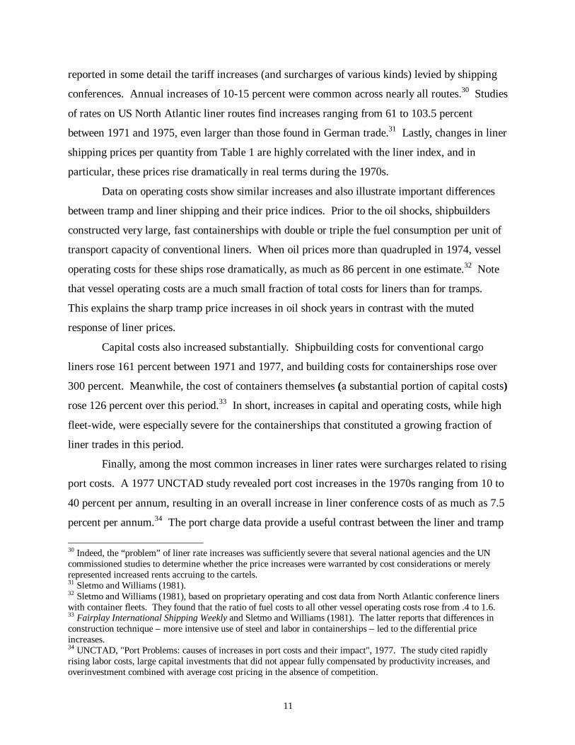
reported in some detail the tariff increases (and surcharges of various kinds) levied by shipping

conferences. Annual increases of 10-15 percent were common across nearly all routes.30 Studies

of rates on US North Atlantic liner routes find increases ranging from 61 to 103.5 percent

between 1971 and 1975, even larger than those found in German trade.31 Lastly, changes in liner

shipping prices per quantity from Table 1 are highly correlated with the liner index, and in

particular, these prices rise dramatically in real terms during the 1970s.

Data on operating costs show similar increases and also illustrate important differences

between tramp and liner shipping and their price indices. Prior to the oil shocks, shipbuilders

constructed very large, fast containerships with double or triple the fuel consumption per unit of

transport capacity of conventional liners. When oil prices more than quadrupled in 1974, vessel

operating costs for these ships rose dramatically, as much as 86 percent in one estimate.32 Note

that vessel operating costs are a much small fraction of total costs for liners than for tramps.

This explains the sharp tramp price increases in oil shock years in contrast with the muted

response of liner prices.

Capital costs also increased substantially. Shipbuilding costs for conventional cargo

liners rose 161 percent between 1971 and 1977, and building costs for containerships rose over

300 percent. Meanwhile, the cost of containers themselves (a substantial portion of capital costs)

rose 126 percent over this period.33 In short, increases in capital and operating costs, while high

fleet-wide, were especially severe for the containerships that constituted a growing fraction of

liner trades in this period.

Finally, among the most common increases in liner rates were surcharges related to rising

port costs. A 1977 UNCTAD study revealed port cost increases in the 1970s ranging from 10 to

40 percent per annum, resulting in an overall increase in liner conference costs of as much as 7.5

percent per annum.34 The port charge data provide a useful contrast between the liner and tramp

30 Indeed, the “problem” of liner rate increases was sufficiently severe that several national agencies and the UNcommissioned studies to determine whether the price increases were warranted by cost considerations or merelyrepresented increased rents accruing to the cartels.31 Sletmo and Williams (1981).32 Sletmo and Williams (1981), based on proprietary operating and cost data from North Atlantic conference linerswith container fleets. They found that the ratio of fuel costs to all other vessel operating costs rose from .4 to 1.6.33 Fairplay International Shipping Weekly and Sletmo and Williams (1981). The latter reports that differences inconstruction technique – more intensive use of steel and labor in containerships – led to the differential priceincreases.34 UNCTAD, "Port Problems: causes of increases in port costs and their impact", 1977. The study cited rapidlyrising labor costs, large capital investments that did not appear fully compensated by productivity increases, andoverinvestment combined with average cost pricing in the absence of competition.

12

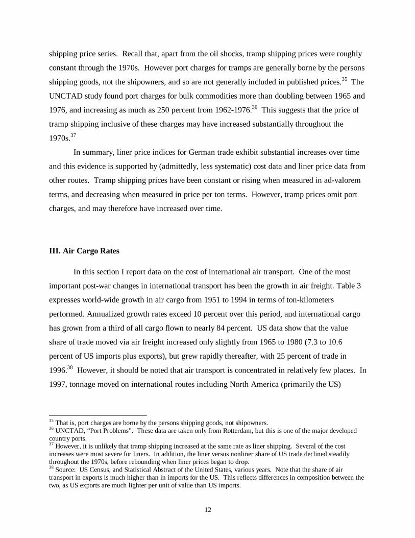
shipping price series. Recall that, apart from the oil shocks, tramp shipping prices were roughly

constant through the 1970s. However port charges for tramps are generally borne by the persons

shipping goods, not the shipowners, and so are not generally included in published prices.35 The

UNCTAD study found port charges for bulk commodities more than doubling between 1965 and

1976, and increasing as much as 250 percent from 1962-1976.36 This suggests that the price of

tramp shipping inclusive of these charges may have increased substantially throughout the

1970s.37

In summary, liner price indices for German trade exhibit substantial increases over time

and this evidence is supported by (admittedly, less systematic) cost data and liner price data from

other routes. Tramp shipping prices have been constant or rising when measured in ad-valorem

terms, and decreasing when measured in price per ton terms. However, tramp prices omit port

charges, and may therefore have increased over time.

III. Air Cargo Rates

In this section I report data on the cost of international air transport. One of the most

important post-war changes in international transport has been the growth in air freight. Table 3

expresses world-wide growth in air cargo from 1951 to 1994 in terms of ton-kilometers

performed. Annualized growth rates exceed 10 percent over this period, and international cargo

has grown from a third of all cargo flown to nearly 84 percent. US data show that the value

share of trade moved via air freight increased only slightly from 1965 to 1980 (7.3 to 10.6

percent of US imports plus exports), but grew rapidly thereafter, with 25 percent of trade in

1996.38 However, it should be noted that air transport is concentrated in relatively few places. In

1997, tonnage moved on international routes including North America (primarily the US)

35 That is, port charges are borne by the persons shipping goods, not shipowners.36 UNCTAD, “Port Problems”. These data are taken only from Rotterdam, but this is one of the major developedcountry ports.37 However, it is unlikely that tramp shipping increased at the same rate as liner shipping. Several of the costincreases were most severe for liners. In addition, the liner versus nonliner share of US trade declined steadilythroughout the 1970s, before rebounding when liner prices began to drop.38 Source: US Census, and Statistical Abstract of the United States, various years. Note that the share of airtransport in exports is much higher than in imports for the US. This reflects differences in composition between thetwo, as US exports are much lighter per unit of value than US imports.

13

constituted 40 percent of all international movements. North American international and

domestic air shipments comprise 53 percent of the world total.39

Cost data for air transport are more sparsely reported than for ocean transport. I rely on

two sources. The first is the World Air Transport Statistics (WATS), which reports world-wide

air freight revenue and ton-kilometers performed each year from 1955-1997. The second is

“Survey of International Air Transport Fares and Rates”, published annually by the International

Civil Aviation Organization (ICAO) between 1973 and 1993. These surveys cover air cargo

freight rates (price per kg for shipment between two cities) for air travel markets around the

world. While the underlying data are not available, the surveys contain rich overviews of the

data that are sufficient for constructing a time series on air cargo costs. Specifically, the Survey

provides information on mean fares and distance traveled for many regions as well as simple

regression evidence to characterize the fare structure. The reported regressions estimate the

elasticity of freight rates with respect to distance for each regional route group in each year. For

most routes and years, distance shipped explains a large portion of the variation in cargo fares, so

rates constructed from the regression will be reasonably informative.40

Annualized growth rates for air freight revenues (totals, and revenues relative to ton-

kilometers and tons shipped) constructed from WATS are reported in Table 4. The data reveal

rapidly growing revenues from 1955-1980, then a significant slowdown through the 1980s prior

to renewed growth in the 1990s. Average revenues per ton-km decline in every period, with

especially rapid decreases of 8-9 percent per annum until 1970, and somewhat slower rates of

decline thereafter. This series can be thought of as a crude measure of price per output unit.

However, the simple average may overstate the true decline in costs. Suppose the cost

technology for air shipping is given by

C a ton kmt= ( )( )β

where at is a time-specific cost shifter. If the elasticity of costs with respect to distance shipped

is less than one, doubling distance shipped results in a decline in average costs per ton-miles.

39 IATA, World Air Transport Statistics.40 Regression R2 of 0.8 to 0.9 are common.

14

WATS data indicates a rapid rise in mean distance shipped over time, so a useful measure of the

cost of shipping requires an estimate of the relevant elasticity.

There are two sources one might use. The first comes from the ICAO Survey, which

reports regressions of (log) cargo rate on the (log) air distance between cities world-wide.41

Using world-wide data, the elasticity of costs per kg with respect to distance is .81 in the earliest

available year, 1973. A second source is US trade data, detailed in the next section. Estimates

for 1974 indicate that the elasticity of costs per kg with respect to distance is 0.5.42 I use these

estimates to construct changes in average revenues correcting for the rise in distance shipped.

This calculation reveals somewhat slower rates of decline compared to the simple average rate.43

The ICAO Survey provides a more detailed source of data on air cargo rates, albeit a

much shorter time series. The regression evidence reported there can be used to evaluate

changes in the level of air freight rates, as well as changes in the structure of rates over time. To

examine changes in the level of rates I construct, for each year and route group, a predicted cargo

rate (dollars per kg) for the mean distance shipment in that route group.44 I deflate this series

using the US GDP deflator, and an index of air-shipped traded goods prices. The latter is used in

place of a more general import price series for two reasons. One, the time series of prices in air-

shipped goods may differ substantially from the overall import series. Two, the series can be

constructed in a way that allows a precise calculation of changes in the ad-valorem freight rates.

To explain, air freight rates are quoted in dollars per kg shipped, so multiplying the rate

by the weight-value ratio of a good immediately yields the ad-valorem rate. The question then

becomes: what is an appropriate weight-value ratio to employ? The aggregate weight-value ratio

is greatly influenced by movements in bulk commodity prices that are never air shipped and so

are not relevant for this calculation. (For US import data, the aggregate weight-value ratio (all

goods) yields ad-valorem rates in excess of 750 percent.) Simply using the weight-value ratio

for air-shipped goods is also problematic because it will understate cost declines. If air prices

decline relative to ocean air, shipment by air becomes feasible for heavier goods. This raises the

observed weight-value ratio. To deal with both problems, I construct a Laspeyres type index 41 The rate is the price per kilogram for shipping a package up42 The much lower distance elasticity from US trade data matches ICAO estimates for route groups involving theUS.43 Of course, this assumes a constant elasticity over time as well as ignoring compositional effects (where airtransport has grown and whether costs have fallen at different rates in those regions).

15

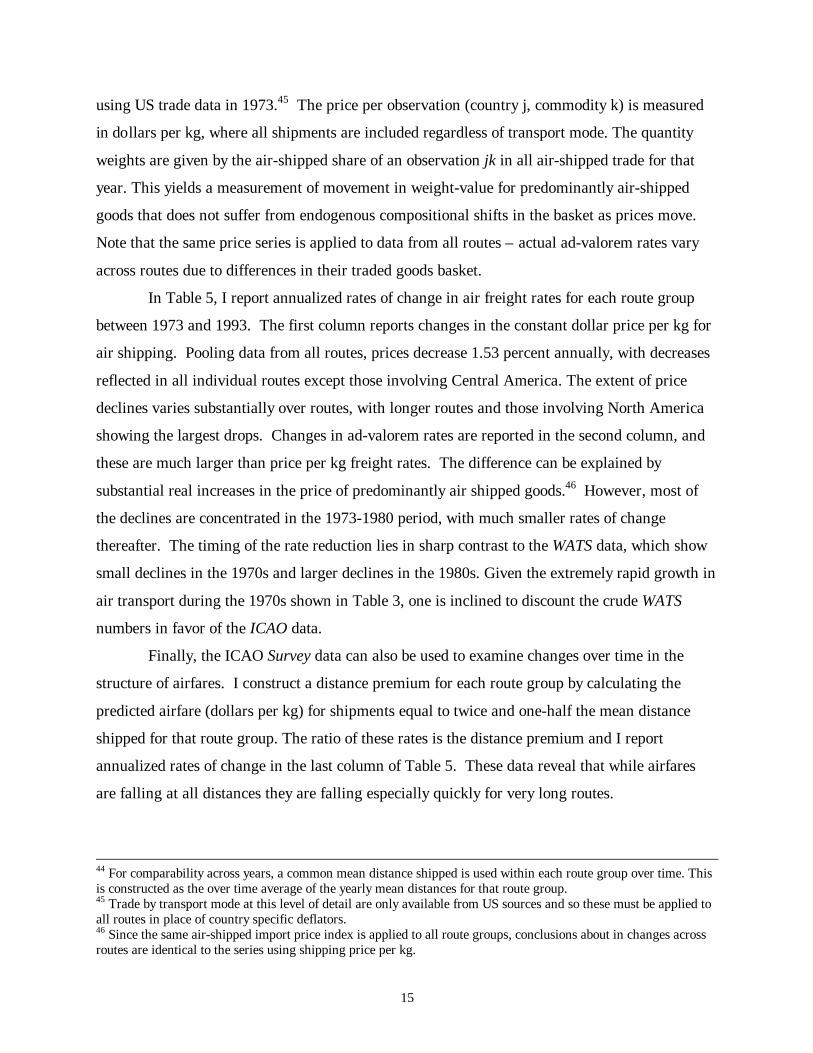
using US trade data in 1973.45 The price per observation (country j, commodity k) is measured

in dollars per kg, where all shipments are included regardless of transport mode. The quantity

weights are given by the air-shipped share of an observation jk in all air-shipped trade for that

year. This yields a measurement of movement in weight-value for predominantly air-shipped

goods that does not suffer from endogenous compositional shifts in the basket as prices move.

Note that the same price series is applied to data from all routes – actual ad-valorem rates vary

across routes due to differences in their traded goods basket.

In Table 5, I report annualized rates of change in air freight rates for each route group

between 1973 and 1993. The first column reports changes in the constant dollar price per kg for

air shipping. Pooling data from all routes, prices decrease 1.53 percent annually, with decreases

reflected in all individual routes except those involving Central America. The extent of price

declines varies substantially over routes, with longer routes and those involving North America

showing the largest drops. Changes in ad-valorem rates are reported in the second column, and

these are much larger than price per kg freight rates. The difference can be explained by

substantial real increases in the price of predominantly air shipped goods.46 However, most of

the declines are concentrated in the 1973-1980 period, with much smaller rates of change

thereafter. The timing of the rate reduction lies in sharp contrast to the WATS data, which show

small declines in the 1970s and larger declines in the 1980s. Given the extremely rapid growth in

air transport during the 1970s shown in Table 3, one is inclined to discount the crude WATS

numbers in favor of the ICAO data.

Finally, the ICAO Survey data can also be used to examine changes over time in the

structure of airfares. I construct a distance premium for each route group by calculating the

predicted airfare (dollars per kg) for shipments equal to twice and one-half the mean distance

shipped for that route group. The ratio of these rates is the distance premium and I report

annualized rates of change in the last column of Table 5. These data reveal that while airfares

are falling at all distances they are falling especially quickly for very long routes.

44 For comparability across years, a common mean distance shipped is used within each route group over time. Thisis constructed as the over time average of the yearly mean distances for that route group.45 Trade by transport mode at this level of detail are only available from US sources and so these must be applied toall routes in place of country specific deflators.46 Since the same air-shipped import price index is applied to all route groups, conclusions about in changes acrossroutes are identical to the series using shipping price per kg.

16

The evidence on air cargo rates provides a marked contrast to the data on ocean shipping.

Aggregate data reveal extremely large declines in costs between 1955 and 1997, while more

detailed survey data reveals smaller, though still substantial, declines from 1973-1993. Changes

in these relative prices provide a highly plausible explanation for the shift toward air transport

shown in Table 2.

IV. Trade Data: US and New Zealand Customs Reports

In this section I use freight data gathered from United States and New Zealand customs

reports.47 In each case, customs authorities report the value of trade inclusive (cif) and exclusive

(fob) of shipping costs. These data have the following advantages. First, they provide a reliable

time series on freight expenditures that can easily be expressed in ad-valorem equivalent terms.

Second, the data allow me to decompose changes in aggregate freight rates into changes in unit

shipping costs and changes in shipping characteristics, including commodity composition,

exporter composition, and goods prices.

The US data come originally from the US Census Bureau, “US Imports of Merchandise”

and cover years 1974-1996. Importers are required to report the cif and fob valuation of imports,

the quantity and weight of the good, and duties paid. Census also reports the country of export, a

highly disaggregated goods classification (TSUSA or in later years, Harmonized System)

shipping mode (sea, land, air), and district of entry and unlading. The New Zealand data are

derived from import shipment data. For years 1965-1986, the publication “New Zealand

Imports” reports cif and fob values of trade at the 2 digit SITC level, aggregated over all

exporting countries, as well as cif and fob values for each exporter, aggregated over all goods.

For years 1988-1997, electronic data sources available from Statistics New Zealand provide

shipment weight and cif and fob trade values by exporting country at the 5-digit SITC level.

Figure 3 reports time series variation in aggregate ad-valorem freight rates for the US and

New Zealand. The US data exhibit declining rates (from 6.4 to 3.6 percent of import value),

while the New Zealand data fluctuate (between 7 and 11 percent of import value) but show no

clear trend. Of course, these aggregate expenditure data are subject to important compositional

effects. The composition hypothesis can be simply illuminated by decomposing the aggregate

17

expenditure on freight rates. Let transportability vary over goods, exporters, and time,

represented by a unique ad-valorem freight rate for each, f jkt , and denote the value of trade in

that observation as V jkt . The aggregate ad-valorem freight rate in each period is given by a

weighted average of commodity x country transportation costs, with weights given by the value

share of each good in trade, SVVjkjk

jkjk

=∑

, or fV f

VS ft

jkt jktjk

jktjk

jkt jktjk

=∑

∑= ∑

This effect can be shown simply in cross-section by comparing the trade-weighted

average freight rate to a simple average rate (i.e. setting shares equal to 1/n for all observations).

Unweighted mean freight rates for the US range between 12 and 15 percent ad-valorem, or

roughly two to three times the weighted rates. Similarly, if trade growth has occurred primarily

in cheaply-shipped commodity groups, this will cause a decline in the aggregate ad-valorem rate.

Consider the following simple characterization of shipping costs. Denote Ps as the unit cost of

shipping ($/ton), Qk as the quantity shipped in units, wk as the weight per unit, and Pk as the unit

price of the good. The freight expenditure F on good k equals the total weight shipped

multiplied by the unit shipping cost. Expressing this as a fraction of the good's value, we have

the ad-valorem freight rate, which is increasing in the unit weight-value ratio for the good.

(1) fFV

P Q wP Q

PwP

kk

k

s k k

k ks

k

k= = =

The top half of Table 6 shows the composition of world-wide trade growth from 1950-

1995, with index numbers representing quantities of total trade and three broad aggregates:

agricultural products, mining products, and manufactures. 48 Trade in manufactured goods has

grown much more rapidly (27-fold) than either agriculture (5-fold) or mining (7-fold) products.

The bottom half of the table shows US imports (1969-1995), split into one-digit SITC categories.

It reports the value share of each category in total trade and two measures of transportability – 47 A broader set of countries would be highly desirable but these are the only countries whose public use trade dataincludes a lengthy time series on shipping costs.

18

the aggregate weight-to-value ratio and aggregate expenditures on freight relative to value in

each category. Easily transported manufactures (SITC 5-9) grow while expensively shipped

commodities (SITC 0-4) shrink.

An estimate of true shipping prices must then separate price effects from compositional

effects. Given the limited detail in the New Zealand data from 1964-86 (freight rates by country,

or freight rates by 2-digit SITC commodity), it is only possible to control for composition using a

standard index number approach. I employ Laspeyres and Pasche price indices, where the

observation price is the ad-valorem freight rate for that country (commodity), with weights equal

to the country (commodity) value share in trade for base years 1964 and 1997, respectively. This

holds fixed the country (commodity) share of trade and allows only prices (freight rates) to vary.

The bottom half of Figure 3 displays price indices for New Zealand compared to the

aggregate freight rate with price indices set equal to the freight rate in base years. Both indices

track the aggregate freight rate closely, departing only in the years furthest from the base. In

each case, the departures tend to flatten the series – the Pasche index pulls initial rates down, and

the Laspeyres index pulls rates up in later years. A price index that holds country composition

constant shows even smaller departures from the trade-weighted average rate.

The US data allow a more detailed exploration of freight rates and their variation over

time. In particular, I use detailed information on shipment characteristics in order to extract a

time series on shipping costs controlling for compositional effects. The model of ad-valorem

freight rates for shipments originating in country j, terminating at port p, in commodity k at time

t is given by

(2) ln ln ln ( ln ) ( ln )f DISTwp

T T T DIST T DISTjkpt jpjkpt

jkptk t t t pj t pj= + + + + + ⋅ + ⋅η 2 2

The regression controls for distance shipped and weight-value, and allows time-invariant

differences across goods in shipping costs. A linear and a quadratic trend, along with trend

interactions with distance are included to capture changes in shipping prices. Results are very

48 These rates refer to growth in the quantity of trade in each category (arrived at by dividing unit values by unitprices). Measuring growth in the value of trade, manufacturing trade grew 100-fold while agriculture and miningtrade grew 15 and 50-fold, respectively. Data are gathered from WTO sources.

19

similar when year and year*distance interactions are employed. Good k refers to a 5-digit SITC

commodity, and the time period spans 1974-1996.

Table 7 reports results of equation 2. The controls enter as expected, with freight rates

rising with weight/value and with distance. Also, the distance and weight/value coefficients are

higher for air transport. This, sensibly, suggests that shipping any particular good from any

particular exporter will be more expensive via air. More interesting are the trend variables, which

reveal an increasing intercept, but a declining distance elasticity over time. This indicates a kind

of rotation in the freight-distance profile – freight rates are rising over short distances, and falling

over long distances. For air cargo, this reproduces the result found in the ICAO Survey data. For

ocean shipping there is a ready technological explanation for the phenomenon – large, fast

containerships provide the greatest cost savings over long routes. A falling distance coefficient

may represent the steadily growing use of containerships in trade.

To evaluate the overall trend in freight rates, I evaluate the regression at the variable

means. At the mean distance shipped, both ocean and air freight rates fell about 60% between

1974 and 1996. However, the US Census Bureau only began collecting freight expenditure data

in 1974 and this is an especially inauspicious beginning year. The New Zealand data and the

tramp shipping indices indicate that shipping prices peaked in this year, and 1973-1974 also

represents the single largest year to year change in the liner shipping index. If these trends are

also present for US trade, the first year of the data corresponds to a local maximum in the price

series, making it difficult to draw broad conclusions about the longer time series.

A few crude calculations drawing on the longer series are possible. For ocean freight, the

New Zealand data, the liner and both tramp indices all show freight rate increases of around 30

percent from 1973-1974. For air freight, ICAO Survey data indicate an average increase of about

8.5 percent between 1973-74 for routes involving the US. I impute ocean and air freight levels

for 1973 by lowering the 1974 levels 30 and 8.5 percent respectively. Compared to the 1973

level, ocean freight prices increase sharply until 1976, then decline steadily. However, they do

not reach the 1973 levels again until 1990. This yields a series that is broadly consistent with the

other ocean freight prices shown thus far -- prices fluctuate until the late 1980s, then decline over

the last decade. Compared to the 1973 level, air freight prices briefly increase, but drop below

1973 levels in 1977, and drop 50 percent by 1996.

20

V. Inland Transport: Indirect Measures

Data on the costs of inland transport are extremely difficult to obtain, except on a case study

basis. The few available studies typically find inland transport charges to be the largest portion

of international shipping expenses. For example a 1968 OECD study finds sea freight for liner

cargoes, including loading and unloading charges, to be between 40 and 60 percent of total door

to door shipping charges. Combining this with estimates that loading and unloading costs equal

as much as half of sea freight charges for liner cargoes, one arrives at a value of only 20 to 30

percent for purely ocean transport. Clearly then, one would like some assessment of the costs of

overland transport.

Two pieces of indirect evidence are available. Liner freight rates include costs of inland

transport related to port costs, while the other series (tramp shipping, customs trade data) do not.

Liner rates have increased relative to the other series, and this relative movement may reveal,

crudely, increases in port costs.

Second, one can indirectly evaluate changes in overland versus ocean shipping prices by

observing changes in relative use of these modes. The US is a large land mass with four

potential entry coasts (Pacific, Atlantic, Gulf, Great Lakes). A European shipper needing to send

goods to California then has several options: place the goods on a very long ocean voyage

through the Panama Canal, or enter the goods on the Atlantic or Gulf Coast and land-ship them

to California. Presumably this decision depends on the relative costs of ocean versus inland

journeys. Is there any evidence that shippers substitute away from ocean-intensive shipping

toward land-intensive shipping?

To measure this, I calculate for each shipment the entry port that would minimize ocean

shipping distance and compare this to the actual port used. The ratio of the two provides a

measure of “excess ocean distance”.49 Especially interesting are cases where a shipper’s

minimum ocean distance port is on an entirely different coast than the port actually employed.

Figure 4 plots excess distance over time for those shipments where the minimum distance and

entry ports are on different coasts. It shows a marked decline in excess distance, that is, a

shortening of ocean voyage legs in favor of longer land distance legs. This is especially striking

21

as estimates from the previous section indicate that the distance costs of ocean transport are

falling over time, making excess distance shipped progressively cheaper.

Of course, a demonstration that inland transportation costs have fallen is not necessarily

an indication that international costs have fallen relative to domestic costs. Domestic

transactions may use domestic transport more intensively than international transactions because

domestic transport is but one component in the overall international transport chain. This would

imply that the costs of international transactions costs actually rise in relative terms when

domestic costs drop. However, domestic transactions have the option to locate internally so as to

minimize these costs, and so may less intensively demand domestic transport.

V. Implications and Extensions

This paper has drawn on an eclectic mix of data to show that the cost of ocean transport

has risen and the cost of air transport has fallen over time. Further, changes in rate structures

indicate a decline in the costs of distant relative to proximate transport. Both changes match

compositional shifts in trade toward air shipping and toward distant partners.

Two challenges remain. First, the data provided here implicitly assume that

transportation services are of homogeneous quality over time, and this will likely concern many

readers. Undoubtedly there have been important technological changes in shipping, but the

difficulty lies in identifying which of these provide improved transport services to importers, and

are not already being measured. More efficient ships ought to yield lower shipping prices;

navigational aids that limit accidents should show up in reduced insurance premiums. Further, it

should be noted that the replacement rate for shipping is very slow; new ships are added at a rate

of approximately 2% of the existing fleet each year, and the average age of the active fleet is 15

years old. Thus, even dramatic technological improvements require decades to be felt fleet-wide.

It also suggests that whatever improvements have occurred, they are not so great as to obsolete

the existing capital stock.

Perhaps the most obvious quality improvement is speed. This is manifest in the switch to

air transport as well as in substantially increased ship speed for ocean liners. A simple-minded

49 Young (1999) performs excess distance calculations for international transit shipping and demonstrates that goodstake very indirect routes. The same appears to be true even for single country shipping.

22

view of the value of time might focus primarily on inventory-holding costs, and these are likely

to be quite small. (A transatlantic crossing at top fleet speeds today might save a week relative

to top fleet speeds four decades ago.) A broader view would focus on why particular goods are

time intensive, and the possibility that faster transport might open up trade in entirely new goods

or lead to entirely new organizations of production. An obvious example is perishable foods, a

more compelling example is trade in intermediate components intended for just-in-time linkage

into a multi-country vertical production chain.

This leads to the second challenge, identifying the role that transportation, narrowly

defined, plays in trade growth and international integration more broadly. One is tempted to

look at the evidence on ocean freight rates and conclude that transport costs cannot plausibly

lead to trade growth since they have not declined! But again, this is too simple. It may be that

compositional changes in the price of transport -- relative reductions in air, overland, and

distance premia -- can tell us a great deal about how trade has grown. They may similarly tell us

much This paper provides simple, suggestive correlations. Careful study is required.

Finally, it may simply be that changes in transportation, narrowly defined, do not much

affect trade growth or international integration. The third challenge then, is to identify trade

barriers, or components of transportation broadly defined, that do matter. This paper is a first

step in that process.

23

References

Baier, Scott, and Bergstrand Jeffrey (1998) "The Growth of World Trade: Tariffs, Transportation Costs, andIntermediate Goods", mimeo, U. Notre Dame

Conlon, R.M. (1982), “Transport Cost and Tariff Protection of Australian Manufacturing”, Economic Record, 73-81.

Evenett, Simon, Djankov, Simeon, and Bernard Yeung (1998) "The Willingness to Pay for Tariff Liberalization",mimeo, University of Michigan.

Finger, J.M. and Yeats, Alexander (1976), “Effective Protection by Transportation Costs and Tariffs: AComparison of Magnitudes”, Quarterly Journal of Economics, 169-176.

Harley, C. Knick, (1980) “Transportation, the World Wheat Trade, and the Kuznets Cycle, 1850-1913”,Explorations in Economic History, 17, 218-250.

Harley, C. Knick, (1988) “Ocean Freight Rates and Productivity, 1740-1913: The Primacy of Mechanical InventionReaffirmed”, Journal of Economic History, 48, 851-876.

Harley, C. Knick, (1989) “Coal Exports and British Shipping, 1850-1913”, Explorations in Economic History, 26,311-338.

Hummels, David (1999), "Toward a Geography of Trade Costs", mimeo, University of Chicago

Hummels, David, Ishii, Jun, and Kei-Mu Yi, (1999) "The Nature and Growth of Vertical Specialization inInternational Trade", mimeo, University of Chicago

Krugman, Paul, (1995), "Growing World Trade: Causes and Consequences", Brookings Papers.

McKinsey and Co., (1967)"Containerization: the Key to Low Cost Transport"

OECD, Maritime Transport

OECD (1968) Ocean Freight Rates as part of Total Transport Costs

Sampson, G.P. and Yeats, A.J. (1977), “Tariff and Transport Barriers Facing Australian Exports” Journal ofTransport Economics and Policy, 141-154.

Sletmo and Williams (1981) Liner Conferences in the Container Age.

Rose, Andrew (1991), "Why Has Trade Grown Faster than Income?" Canadian Journal of Economics, Vol 24.

Tolofari (1986), Open Registry Shipping

UNCTAD, Review of Maritime Transport

Waters, W.G. (1970), “Transport Costs, Tariffs, and the Patterns of Industrial Protection, American EconomicReview, 1013-20.

Yeats, Alexander (1978) "On the Accuracy of Partner Country Trade Statistics" Oxford Bulletin of Economics andStatistics, vol 40, no. 4.

24

Appendix I: Data

Shipping Indices

All data on shipping indices were collected from various issues of UNCTAD, “Review of

Maritime Transport” and various issues of OECD, “Maritime Transport”. These publications

collected the data from the sources noted below. For details on the precise construction of the

indices see UNCTAD, “Level and structure of freight rates, conferences practices and adequacy

of shipping services” or the original sources.

Norwegian shipping indices (tramp time charter and tramp voyage charter) are compiled

by the Norwegian Shipping News, later, Shipping News International. The tramp time charter

index for Norway reports an index of the cost of employing entire vessels for a period of time

less than nine months. Coverage is worldwide, and the use of the ships (i.e. which goods they

will transport) is ignored. The index includes vessels of varying size and speed. The weighting

used for various ship classes was originally based on 1947, and was updated to a new base year

in 1967 (base year 1965) and again in 1972 (base year 1971).

The voyage charter index for Norway is a weighted index number of the cost of shipping

a given quantity of goods. The basket includes bulk commodities such as grains, coal, sugar iron

ore, phophate, scrap iron, rice, fertilizers and copra, with each commodity represented with

several shipping routes. The prices for a specific commodity are averaged across routes, and the

commodity basket is constructed using weights for each commodity. Weights originally used a

1947 base year, updated in 1967 to a 1965 base year.

The liner shipping index for Germany is compiled by the German Ministry of Transport.

It differs from other series in three important respects. First, it covers prices charged by liner

conferences, not prices prevailing in spot shipping markets. Second, its covers only those ships

loading and unloading in Germany and Netherlands. (The Netherlands is included as a

significant fraction of German imports land in the Netherlands and are transported into Germany

via inland freight.) Third, it covers both dry bulk and general cargo, the latter of which includes

containerized shipping and merchandise of all sorts. The weighting of the index (both

commodities within dry bulk and general cargo and dry bulk v. general cargo) was based on

25

1954, and updated in 1968, 1985, 1990, and 1996 to include base years of 1965, 1980, 1985, and

1991, respectively.

All of the series are updated to new base years for weighting schemes. To provide

continuity of the series, old and new series are joined on common years so that the entire series

employs a common unit base year. That is, if 1947 – 1966 are based on 1947=100, and 1967-

1997 are based on 1965=100, the values from 1967 to 1997 are divided by the 1965 price to get

all series in a common year. Of course, this is not the same thing as using a common base year

for the weighting, and some of the changes in the time series may result from weighting changes.

At least for the tramp shipping indices, the weighting scheme does not appear to matter overly

much. Indices collected by the Norwegian Shipping News and the UK Chamber of Shipping

tightly covary – the correlation coefficient between voyage rates collected by each is .87, and the

correlation between voyage and time rates is .93 to .95.

Trade Data

The US trade data come from the US Census Bureau, “Imports of Merchandise” CD-

ROMS, various editions. See Feenstra (1997) for details on a subset of these data.

The New Zealand data from 1964-1986 come from the serial “New Zealand Imports”.

Statistics New Zealand provided data from 1988-1997 in electronic format. The break in the

series provides two difficulties. First, the coding scheme changes from SITC Revision 1 to

Revision 2 in 1979 and to Revision 3 in 1988, and this may produce some comparability

problems in the series. However, higher revisions have been concorded backwards to Revision1,

and goods are reported at the 2-digit level, so this is a fairly clean mapping. Second, the data

source changes between periods, and the fob valuation of goods may not be the same in each

case. Specifically, from 1964-1986 fob prices are based on goods valuation in the exporting

country, and not directly from importer's declarations of the value of the goods as in 1988-1997.

This results in certain goods having negative transport costs in some years. There are particular

SITC codes for which this is a common problem. These are dropped from the calculations

reported in the paper, though all the results are quite similar if these sectors remain in.

26

Appendix II: IMF CIF/FOB Ratios

In this section, I discuss the measurement of transportation costs using importer cif/fob

ratios constructed from IMF sources, including the Direction of Trade Statistics (DOTS) and the

International Financial Statistics (IFS). Both report trade flows using as a primary source the

UN's COMTRADE database supplemented in some cases with national data sources. While the

measurement of transportation costs are not the primary purpose of these publications, DOTS and

IFS are sometimes used to this end.50 In principle, exporting countries report trade flows

exclusive of freight and insurance (fob), and importing countries report flows inclusive of freight

and insurance (cif). Comparing the valuation of the same aggregate flow reported by both the

importer and exporter yields a difference equal to transport costs. The advantage of using these

data is breadth of coverage: they are available for many years (1948-1997) and for many

countries (41 countries in every year, and over 100 countries are represented at some point in the

data). The disadvantages of using these data are serious quality problems (discussed below) and

depth of coverage (no data on commodity and country-pair cif/fob ratios).51

Figure A.1 reports a world-wide value for transportation costs as measured by the ratio of

CIF to FOB valuation of trade. Two possible conclusions suggest themselves. One,

transportation costs have declined precipitously – from 13 percent of trade to virtually zero from

1949 to 1995. Two, transportation costs were almost exactly constant at 3.5 percent of trade

from 1953 to 1997. These data can also be used to examine trends in total transport costs in

imports for each country. Out of 109 countries, 36 show a significant downward trend, 39 show a

significant upward trend, and 34 exhibit no trend.

Unfortunately, the IMF data suffer from severe quality problems and broad inferences

based on these numbers may be unwarranted. There are three serious problems. First, small

discrepancies in the report of the importer or exporter yield large changes in cif/fob ratios. This

50 Several recent papers, Baier and Bergstrand (1998), and Evenett, Djankov and Yeung (1998) use IMF data instudies of the role of transportation costs in world trade. Harrigan () employs similar data from the OECD in workexamining measures of open-ness. Finally, the “Review of Maritime Transport” perhaps the most comprehensivesource of data on international transport cites these data as a primary (and only systematic) source for ad-valoremshipping costs.51 Commodity and country-pair coverage could be extracted from the original data source, UN COMTRADE data.However, quality problems that are severe in aggregate data become truly execrable in country-pair and commoditydata.

27

is easy to see by examining successive DOTS yearbooks. Each yearbook reports multiple

overlapping years, with later years attempting to reconcile previous discrepancies. These

changes are usually small relative to total trade, with variations no greater than one to two

percent of trade annually. However, the changes can be large relative to cif/fob ratios.52 As a

consequence, the measured value of transport costs for a single year swings wildly about in

different yearbooks. For example, the US cif/fob ratio for 1970 is reported variously as 1.13,

1.09, or 1.06, depending on which edition of the yearbook is consulted.

Second, exporter and importer reports of a trade flow may vary for reasons unrelated to

shipping costs. It is well known that there are serious quality problems with export statistics as

few countries make a concerted effort to measure outflows carefully. In a careful study of this

problem, Yeats (1978) decomposes variation in the COMTRADE cif/fob factors into a transport

cost component and other variation. The cif/fob ratio in the COMTRADE database is constructed

using exporter (fob) reports, and US (cif) reports. US Census data also allows construction of

cif/fob ratios, but these come directly from shipment documentation in which importers must

report both the cif value and the explicit cost incurred in shipping. Assuming that the Census

data is the true measure of shipping costs, Yeats matches the COMTRADE data to the US Census

data for various goods and countries, and finds that much of the COMTRADE data variation is

unrelated to true shipping costs. These ratios are especially noisy in developing country export

data. However, Yeats also shows that these quality problems are less severe in more aggregated

data. This leaves open the possibility that a time series on transportation costs drawn from

aggregate data may contain useful information.

Third, and most troubling, for many pairings only one partner reports data and these

constraints force the IMF to construct cif/fob ratios for most of the countries and years. This

problem is severe in the UN COMTRADE data. Between 1962 and 1983, the data contain

reports on aggregate trade flows from both partners for fewer than 40 percent of the bilateral

pairings. Dropping those bilateral pairs with an implied negative transport cost (cif/fob ratios less

than one), the data contain reports from both partners for fewer than 30 percent of pairings. Of

course, the problem is much worse for trade reported at the commodity level, which raises the

troubling question of the accuracy of the aggregate trade figures.

52 Starting with a cif/fob ratio of 1.06, increase the importer’s cif value of trade by 1.5 percent and decrease theexporter’s fob value by 1.5 percent. The cif/fob ratio becomes 1.09, a change of 50 percent.

28

In these cases, the IMF is forced to construct the cif/fob ratio using only one report. The

somewhat sparse documentation in DOTS reports that a 10% increment over the fob value is

used to construct the cif value or, alternatively, a 9% reduction from the cif value is used to

construct the fob number.53 This adjustment is applied to all country pairs and all time periods

for which paired data are not available. (Though it appears that higher markups were used for

some petroleum exporters in some years.)

This imputation pattern may explain two otherwise interesting facts in the IMF data.

First, the mean and median importer cif/fob ratios are not declining over time because for the

majority of countries, a constant cif/fob ratio is imputed. Second, imputation may pull cif/fob

ratios down over time even if transportation costs are constant. Actual cif/fob ratios for

developing country trade are much higher than the 10% imputation factor because much of this

trade takes place in expensively shipped bulk commodities. Data quality on exports is worsening

in developing countries. This forces an increased use of imputation that causes the cif/fob ratios

to decline for importers of bulk commodities. Unfortunately, the documentation does not allow

the user to carefully track where imputations have occurred, which countries they affect, or their

time series properties. We know only that the data are pregnant with these corrections.

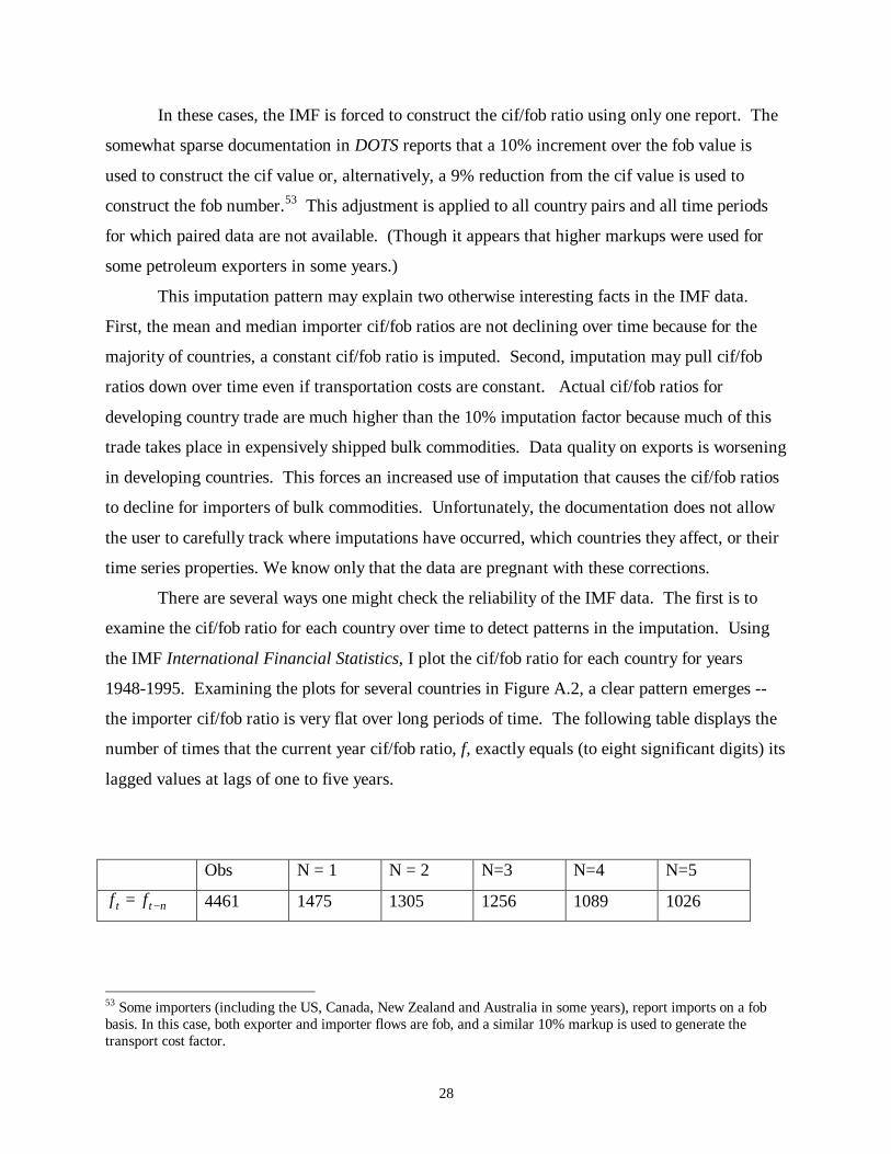
There are several ways one might check the reliability of the IMF data. The first is to

examine the cif/fob ratio for each country over time to detect patterns in the imputation. Using

the IMF International Financial Statistics, I plot the cif/fob ratio for each country for years

1948-1995. Examining the plots for several countries in Figure A.2, a clear pattern emerges --

the importer cif/fob ratio is very flat over long periods of time. The following table displays the

number of times that the current year cif/fob ratio, f, exactly equals (to eight significant digits) its

lagged values at lags of one to five years.

Obs N = 1 N = 2 N=3 N=4 N=5

f ft t n= − 4461 1475 1305 1256 1089 1026

53 Some importers (including the US, Canada, New Zealand and Australia in some years), report imports on a fobbasis. In this case, both exporter and importer flows are fob, and a similar 10% markup is used to generate thetransport cost factor.

29

Nearly 25 percent of observations are identical to their five-year lags. This actually understates

the constancy of these numbers since data for some countries alternates between fixed values, or

returns to a constant value after a few years of variation (see Iceland and Ireland in Figure A2).

To emphasize this, I calculate the modal value of the cif/fob ratio for each country and count the

number of year observations equal to that modal value. Over the whole sample, approximately

one-third of all observations for a country exactly equal that country's modal value, and around

half of all observations equal the modal value rounded to four digits.

Recall, to construct the cif/fob ratios I collect two supposedly independent series, imports

(cif) and imports (fob), from the IFS. Since very small discrepancies in either number will

change the ratio substantially, it is clear that a large fraction of this data is imputed. That is, a

fixed cif/fob ratio is combined with a known cif flow to generate an imputed fob flow (or vice

versa).

However, not all countries display such obvious signs of imputation. To check the

reliability of the IMF's data for these countries, national data sources are useful. Both the United

States and New Zealand require shippers to report measures of trade valued with and without

freight and insurance costs on their import documentation. Taking the national data as the

accurate source, the IMF DOTS yearbook data badly mismeasure both US and New Zealand

transport costs, by a factor of two or more in some cases. However, the IMF data taken from IFS

seems quite accurate for the US beginning in 1974 -- the year that US national sources began

reporting both cif and fob values of the flow. A similar pattern holds in New Zealand's data.

The IMF data taken from the IFS match New Zealand's national sources fairly well beginning in

1963 -- the year that national sources begin reporting both cif and fob values of the flow. In both

cases, the IMF data displays a discrete jump from the previous trend in the year that national data

become available.

Despite data quality problems, is there any information on the time series properties of

transportation costs that can be extracted from the IMF data? This is a hard question to answer,

as it is not clear for which countries the IMF has accurate data and for which they have relied on

wholesale imputation. The world cif/fob ratio accords well with conventional wisdom regarding

transportation costs. And, in those cases where it is possible to verify the IMF data against

national sources, they appear accurate. (Although one suspects that the match between the IFS

and national source data comes from using the relatively accurate US and New Zealand national

30

data sources to correct poorly measured exporter (fob) reports. Essentially, the IMF data may be

accurate because they discard their usual methodology in favor of using US data.) However, the

sort of imputation displayed in Figure A.2 makes variation in IMF cif/fob ratios completely

uninformative for most countries and suspect for the rest.

Figure 1 -- Tramp Shipping Rates

Commodity price deflator

50

75

100

125

150

175

200

225

250

1950 1955 1960 1965 1970 1975 1980 1985 1990 1995

TIMEVOYAGE

GDP deflator

25

50

75

100

125

150

175

1950 1955 1960 1965 1970 1975 1980 1985 1990 1995

TIMEVOYAGE

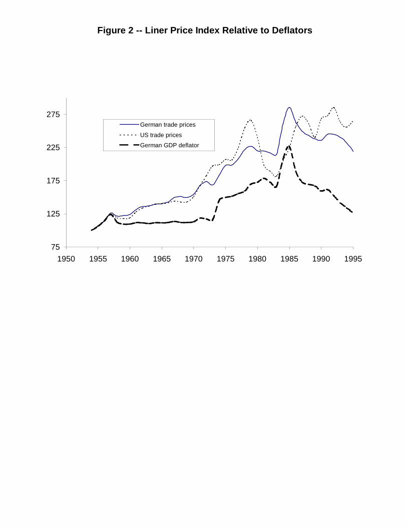
Figure 2 -- Liner Price Index Relative to Deflators

75

125

175

225

275

1950 1955 1960 1965 1970 1975 1980 1985 1990 1995

German trade prices

US trade prices

German GDP deflator

Figure 3 -- Aggregate Freight Expenditures

0

2

4

6

8

10

12

64 68 72 76 80 84 88 92 96

US, NZ Aggregate Freight Expenditures

Frei

ght e

xpen

ditu

res

(% o

f val

ue, w

eigh

t)

US aggregate

New Zealandaggregate#REF!

6

7

8

9

10

11

12

13

64 68 72 76 80 84 88 92 96

Price Indices for New Zealand Freight

Frei

ght e

xpen

ditu

res

(% o

f val

ue)

laspeyres

aggregate freight/value

pasche

0

2

4

6

8

10

12

64 68 72 76 80 84 88 92 96US, NZ Aggregate Freight Expenditures

Frei

ght e

xpen

ditu

re (%

of v

alue

, wei

ght)

New ZealandaggregateUS aggregate

#REF!

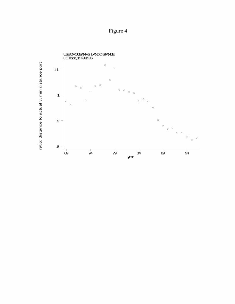
Figure 4

USE OF OCEAN VS. LAND DISTANCEUS Trade, 1969-1996

ratio

: dis

tance

to a

ctual v

. m

in d

ista

nce

port

year69 74 79 84 89 94

.8

.9

1

1.1

Table 1 -- Liner Rates for Specific Commodities/Routes

COMMODITY ROUTE 1963 1965 1970 1975 1980 1985 1990 1996Rubber Malaysia-Europe 7.6 13.3 10.5 18.5 8.9 .. 15.5 8.9Jute Pakistan-Europe 22.6 25.4 12.1 19.5 19.8 6.4 21.2 15.5Cocoa Beans Ghana-Europe 3.3 4.1 2.4 3.4 2.7 1.9 6.7 6.3Coconut Oil Sri-Lanka - Europe 11.2 7.2 8.9 9.1 12.6 12.6 6Tea Sri-Lanka - Europe 5.8 6.3 9.5 10.4 9.9 6.9 10 5.6Cocoa Beans Brazil-Europe 6.4 13.1 7.4 8.2 8.6 6.9 11 6.6Coffee Brazil-Europe .. .. 5.2 9.7 6 5 10 2.6Coffee Colombia - Europe .. .. 4.5 6.3 4.4 6.1 7.4 4.9

COMMODITY ROUTE 1963 1965 1970 1975 1980 1985 1990 1996Rubber Malaysia-Europe 130 206 111 194 155 106 99Jute Pakistan-EuropeCocoa Beans Ghana-Europe 60 47 41 77 88 41 68 64Coconut Oil Sri-Lanka - Europe 88 65 64 62 97 64 0 25Tea Sri-Lanka - Europe 217 221 217 244 250 148 184 80Cocoa Beans Brazil-Europe 107 124 122 185 254 138 96 63Coffee Brazil-Europe 129 192 238 110 104 51Coffee Colombia - Europe 111 125 174 134 77 95

source: UNCTAD, Review of Maritime Transport, IMF International Financial Statistics

Ad-Valorem Rates: Shipping Price Relative to Goods Prices

Quantity Rates: Shipping Price per ton (constant $)

Table 3: Growth in International Air Transport

Int'l Cargo as a %Year All flights International of Total

1951 910 325 35.71955 1300 470 36.21960 2170 990 45.61965 4960 2590 52.21970 10460 6300 60.21975 17100 11300 66.11980 29130 20260 69.61985 39310 28920 73.61990 59163 46241 78.21994 76530 64090 83.7

Annualized Growth Rates1951-1994 10.6 12.8

year Ocean Air Land Ocean Air Land

1965 69.9 6.2 23.9 61.6 8.3 30.11970 62.0 8.6 29.4 57.0 13.8 29.21975 65.5 9.2 25.3 58.9 14.1 27.01980 68.6 11.6 19.8 54.8 20.9 24.31985 60.4 14.9 24.8 43.0 24.5 32.41990 57.2 18.4 24.4 38.4 28.1 33.51994 51.2 21.6 27.3 34.7 29.3 36.0

Sources: IATA, "World Air Transport Statistics", US Census, "US Imports", Statistical Abstract of the US

Imports Exports

World-wide Growth in Air Cargo

Ton-kms performed (mill)

US Trade by Transport Mode (% of value)

Revenueston-km ton

b=.81 b=.51955-1960 5.7 -9.0

1960-1970 10.1 -8.5

1970-1980 10.3 -1.8 1.2 -0.5 0.1

1980-1990 1.7 -6.3 -5.1 -6.1 -5.7

1990-1996 5.1 -3.0 -2.1 -2.8 -2.5

Source: IATA, World Air Transport Statistics

Note:Final column assumes costs = a_t * ton * (km)^bb=.81 estimate from ICAO Survey, all data worldwide, 1973b = .5 estimate from US import data, air mode only, 1974

Average Revenues per Avg rev per ton-kmcontrolling for distance elasticity

Table 4 -- World-Wide Air Freight Revenue(Rates of Change by Decade)

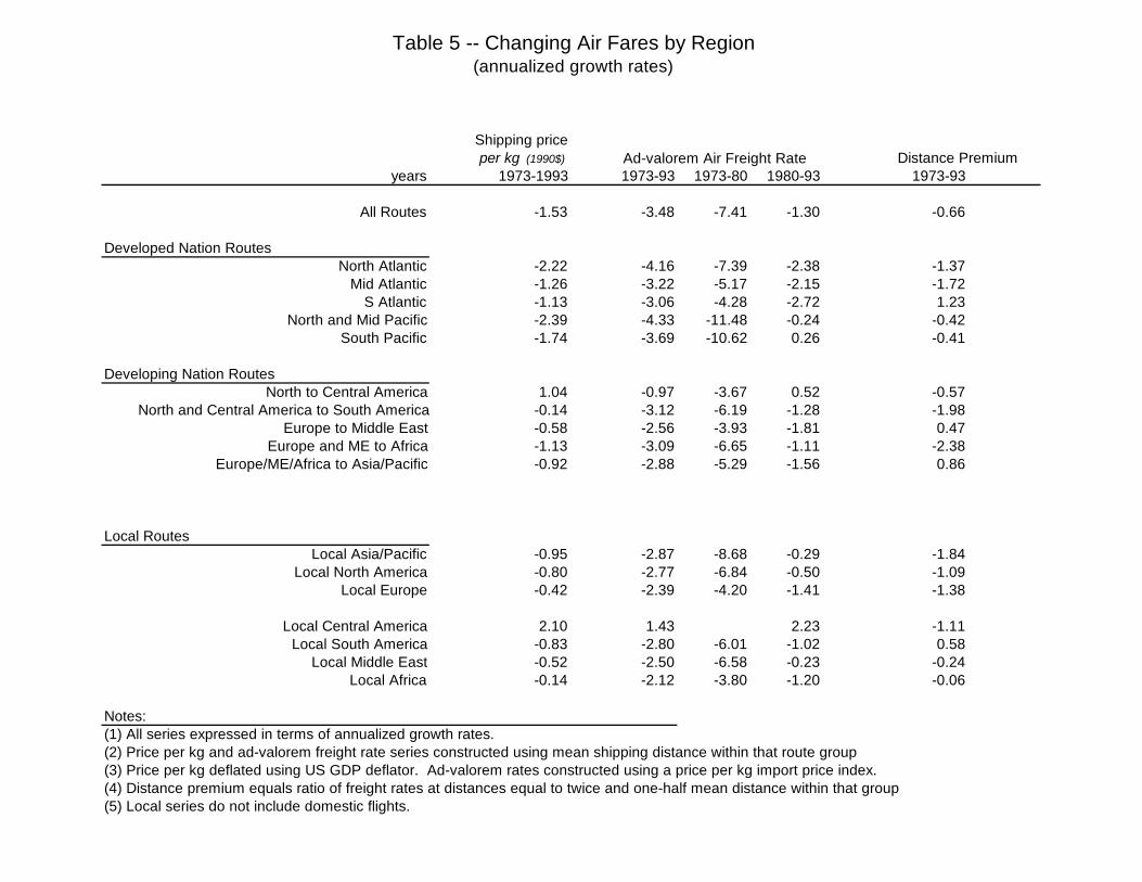
Table 5 -- Changing Air Fares by Region(annualized growth rates)

Shipping priceper kg (1990$) Distance Premium

years 1973-1993 1973-93 1973-80 1980-93 1973-93

All Routes -1.53 -3.48 -7.41 -1.30 -0.66

Developed Nation RoutesNorth Atlantic -2.22 -4.16 -7.39 -2.38 -1.37

Mid Atlantic -1.26 -3.22 -5.17 -2.15 -1.72S Atlantic -1.13 -3.06 -4.28 -2.72 1.23

North and Mid Pacific -2.39 -4.33 -11.48 -0.24 -0.42South Pacific -1.74 -3.69 -10.62 0.26 -0.41

Developing Nation RoutesNorth to Central America 1.04 -0.97 -3.67 0.52 -0.57

North and Central America to South America -0.14 -3.12 -6.19 -1.28 -1.98Europe to Middle East -0.58 -2.56 -3.93 -1.81 0.47

Europe and ME to Africa -1.13 -3.09 -6.65 -1.11 -2.38Europe/ME/Africa to Asia/Pacific -0.92 -2.88 -5.29 -1.56 0.86

Local RoutesLocal Asia/Pacific -0.95 -2.87 -8.68 -0.29 -1.84

Local North America -0.80 -2.77 -6.84 -0.50 -1.09Local Europe -0.42 -2.39 -4.20 -1.41 -1.38

Local Central America 2.10 1.43 2.23 -1.11Local South America -0.83 -2.80 -6.01 -1.02 0.58

Local Middle East -0.52 -2.50 -6.58 -0.23 -0.24Local Africa -0.14 -2.12 -3.80 -1.20 -0.06

Notes: (1) All series expressed in terms of annualized growth rates. (2) Price per kg and ad-valorem freight rate series constructed using mean shipping distance within that route group(3) Price per kg deflated using US GDP deflator. Ad-valorem rates constructed using a price per kg import price index. (4) Distance premium equals ratio of freight rates at distances equal to twice and one-half mean distance within that group(5) Local series do not include domestic flights.

Ad-valorem Air Freight Rate

Table 6: Composition of Trade Growth

Total Agriculture Mining Manufactures1950 9 26 18 51960 18 41 39 111970 41 61 77 291980 68 86 91 581990 100 100 100 1001995 135 125 124 137

source: WTO

% Change ad-valoremSITC Commodity 1969 1995 1969-95 (kg/$) freight rate

0 Food & Live Animals 12.3 3.4 -72.3 0.96 7.641 Beverages & Tobacco 2.4 0.7 -69.0 0.67 7.052 Crude Materials 9.8 3.1 -67.9 6.90 7.633 Mineral Fuels 8.2 8.4 1.7 3.43 6.884 Animal & Vegetable Oils 0.4 0.2 -45.5 1.01 6.055 Chemicals 3.0 4.8 57.0 0.94 4.956 Manufactures (by material) 23.0 12.7 -45.0 0.89 4.857 Machinery & Transport Equip 26.8 46.2 72.2 0.06 2.258 Misc Manufactures 10.5 16.5 57.5 0.09 4.37

World Merchandise Exports Volume, 1950-1995(Index numbers, 1990=100)

Value Share in US Imports Transportability (1995)

US Imports: Commodity Shares and Transportability

Coef. Std. Err Coef. Std. Err Coef. Std. Err

Weight/value 0.420 0.001 0.518 0.001 0.326 0.001

Distance 0.256 0.005 0.508 0.006 0.256 0.005

Distance * trend -0.022 0.001 -0.017 0.001 -0.016 0.001

Distance * trend^2 0.001 0.000 0.000 0.000 0.000 0.000

Trend 0.179 0.009 0.128 0.011 0.127 0.008

Trend^2 -0.007 0.000 -0.004 0.000 -0.004 0.000

constant -3.981 0.043 -4.827 0.055 -3.894 0.041

Dep var is ad-valorem freight rate from exporter j, port p, commodity k, time t.

Regressions include commodity fixed effects

OCEAN AIR BOTH

Table 7 --Freight Rates Over Time(US Imports 1974-1996)

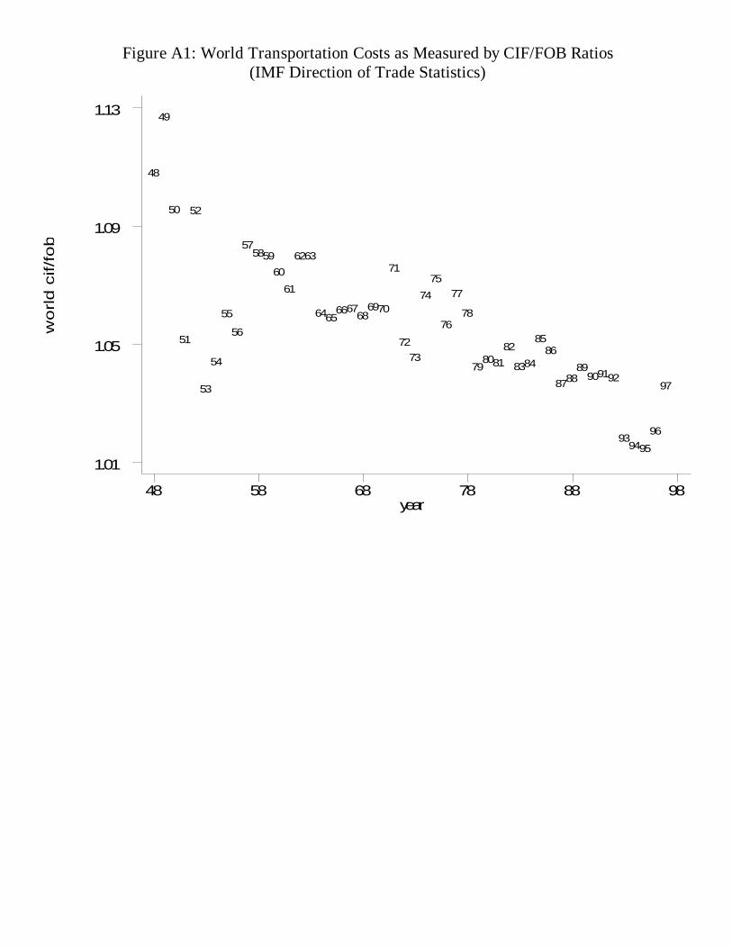
Figure A1: World Transportation Costs as Measured by CIF/FOB Ratios(IMF Direction of Trade Statistics)

wo

rld

cif/

fob

year48 58 68 78 88 98

1.01

1.05

1.09

1.13

48

49

50

51

52

53

54

55

56

575859

60

61

6263

64656667

686970

71

7273

74

75

76

77

78

798081

82

8384

8586

878889

909192

939495

96

97

Table A1 -- Nominal Values of Shipping Price Indices

Liner indexVoyage Composite

NSN UKCS NSN GMT BFI GMT1952 113 100 1151953 88 61 681954 94 72 88 1001955 130 130 140 1081956 152 173 197 1191957 125 120 139 1321958 78 56 64 1221959 79 56 65 1201960 82 65 74 1221961 84 73 81 1271962 78 58 65 1311963 85 69 79 1331964 86 78 88 1381965 90 88 99 1421966 86 87 88 1481967 85 85 88 1521968 83 91 92 1531969 77 92 88 1551970 107 165 130 1621971 73 85 103 1791972 67 89 108 1871973 146 230 237 1991974 196 258 310 2661975 128 114 176 2901976 121 117 180 3051977 120 95 169 3251978 126 134 201 3421979 161 228 284 3791980 192 312 392 4061981 176 235 344 4481982 143 121 210 4561983 153 118 197 4541984 156 144 185 5791985 150 124 183 100 100 6461986 142 106 156 79 5381987 157 163 225 112 4941988 176 263 340 118 152 4901989 184 297 347 139 170 4971990 178 341 106 149 4861991 185 121 175 5101992 176 96 132 5041993 176 125 154 4911994 181 114 163 4781995 203 124 218 4581996 174 88 145 4741997 176 160 495

NSN - Norwegian Shipping News; UKCS - UK Chamber of ShippingGMT- German Ministry of Transport; BFI - Baltic Freight Index (Baltic Freight Exchange)

Tramp Charters Shipping IndicesTime