Hau, Kah Wai (2003) Application of a three-surface ...

TABLE OF CONTENTS

ABSTRACT................................................................................................................ I

ACKNOWLEDGEMENTS .....................................................................................II

LIST OF TABLES .................................................................................................. III

LIST OF FIGURES ................................................................................................ IV

LIST OF SYMBOLS ................................................................................................X

1 INTRODUCTION..............................................................................................1

1.1 BACKGROUND .........................................................................................1

1.2 RESEARCH METHODOLOGY.................................................................4

1.3 STRUCTURE OF THESIS..........................................................................4

2 LITERATURE REVIEW .................................................................................6

2.1 INTRODUCTION .......................................................................................6

2.2 SOIL MECHANICS ....................................................................................6

2.2.1 Elasticity ..............................................................................................6

2.2.2 Plasticity ..............................................................................................8

2.2.3 Critical State ........................................................................................9

2.2.4 Cam clay ............................................................................................12

2.2.5 Modified Cam clay .............................................................................13

2.2.6 Shortcomings of Cam clay and Modified Cam clay...........................16

2.2.7 Advanced Models ...............................................................................23

2.2.8 Cyclic Loading Models ......................................................................25

2.2.9 Earth Pressure Coefficient at Rest.....................................................29

2.3 PAVEMENT ENGINEERING..................................................................32

2.3.1 Pavement Types and Failure Modes..................................................32

2.3.2 Resilient Deformation Models ...........................................................35

2.3.3 Permanent Deformation Models........................................................39

2.3.4 Stress History of a Pavement .............................................................40

2.3.5 Current UK Flexible Pavement Design Methods ..............................43

2.4 NUMERICAL MODELLING ...................................................................44

2.4.1 Introduction........................................................................................44

2.4.2 Basic Finite Element Concepts ..........................................................45

2.4.3 Critical State Program (CRISP) ........................................................48

2.5 SUMMARY...............................................................................................49

3 PRELIMINARY STUDY – EVALUATION OF THE TWO AND THREE-

SURFACE KINEMATIC HARDENING MODELS ...........................................51

3.1 INTRODUCTION .....................................................................................51

3.2 MODEL DESCRIPTION ..........................................................................51

3.2.1 Translation Rule.................................................................................54

3.2.2 Hardening Modulus ...........................................................................58

3.2.3 Determination of Model Parameters .................................................63

3.3 ONE-DIMENSIONAL LOADING, UNLOADING AND RELOADING 65

3.4 CYCLIC LOADING..................................................................................68

3.4.1 Model Predictions for Repeated Loading ..........................................69

3.4.2 Accumulation of Negative Shear Strain.............................................75

3.5 THREE-LAYER PAVEMENT: RESILIENT AND PERMANENT

DEFORMATIONS ................................................................................................81

3.5.1 Resilient Deformation: BISAR vs CRISP...........................................81

3.5.2 Permanent Deformation.....................................................................88

3.6 SUMMARY...............................................................................................91

4 FORMULATION OF A SIMPLE NON-ASSOCIATED THREE-

SURFACE KINEMATIC HARDENING MODEL..............................................92

4.1 INTRODUCTION .....................................................................................92

4.2 NON-SYMMETRICAL FLOW RULE.....................................................93

4.3 THE NON-ASSOCIATED THREE-SURFACE KINEMATIC

HARDENING MODEL.........................................................................................95

4.3.1 Model Description .............................................................................96

4.3.2 Stress-dilatancy Rule .........................................................................96

4.3.3 Hardening Rule ..................................................................................99

4.3.4 Yield Surface and Plastic Potential in Deviatoric Plane.................101

4.3.5 Justification of ∂M/∂θ = 0................................................................103

4.3.6 Generalisation of Model, Finite Element Implementation and

Validation of the New Model in CRISP ...........................................................106

4.3.7 Evaluation of the New Model...........................................................109

4.3.8 Modification of the Hardening Modulus..........................................116

4.3.9 Determination of Parameters ..........................................................118

4.4 SUMMARY.............................................................................................119

5 EXPERIMENTAL VALIDATION OF THE NON-ASSOCIATED

THREE-SURFACE KINEMATIC HARDENING MODEL ............................121

5.1 INTRODUCTION ...................................................................................121

5.2 TRIAXIAL TEST ....................................................................................121

5.2.1 Description of the Triaxial Apparatus .............................................122

5.2.2 Soil Used in the Experimental Test ..................................................124

5.2.3 Sample Preparation .........................................................................124

5.2.4 Specimen Set Up and Test Procedure ..............................................126

5.2.5 Analysis of Data ...............................................................................128

5.3 DETERMINATION OF MODEL PARAMETERS................................128

5.3.1 Model Parameters............................................................................129

5.3.2 Parametric Study .............................................................................135

5.4 REPEATED LOADING RESULTS AND MODEL PREDICTIONS....143

5.5 SUMMARY.............................................................................................147

6 FULL-SCALE PAVEMENT ANALYSIS ...................................................149

6.1 INTRODUCTION ...................................................................................149

6.2 PAVEMENT FOUNDATION DESIGN.................................................150

6.2.1 Resilient Deformation During Construction Stage..........................151

6.2.2 Rut Depth of Unpaved Roads Under Construction Traffic..............155

6.3 THREE-LAYER PAVEMENT ANALYSIS – EFFECT OF GRANULAR

LAYER THICKNESS AND ASPHALT LAYER THICKNESS .......................157

6.4 SUMMARY.............................................................................................161

7 CONCLUSIONS AND SUGGESTIONS FOR FUTURE RESEARCH...163

7.1 SUMMARY AND CONCLUSIONS ......................................................163

7.2 RECOMMENDATIONS FOR FUTURE WORK ..................................168

APPENDIX.............................................................................................................170

REFERENCES.......................................................................................................172

ABSTRACT Little effort has been made to apply the Critical State Soil Mechanics concept to the

prediction of pavement response. The aim of this research is to apply soil mechanics

principles, particularly the kinematic hardening concept, to the prediction of the

response of lightly trafficked pavements to repeated loading. For this purpose, the

finite element critical state program CRISP is used.

A comparison is made between the predictions given by the three-surface kinematic

hardening (3-SKH) model and a layered elastic analysis BISAR for the resilient

deformation produced by repeated loading of a thinly surfaced pavement, and the

models are found to be in good agreement. The ability of the 3-SKH model to

predict soil behaviour under cyclic loading, and under one-dimensional loading,

unloading and reloading is also evaluated. A comparison between model predictions

and experimental data obtained by other researchers shows that the 3-SKH model

over-predicts the value of K0,nc and hence shear strain during monotonic loading.

This problem is magnified when the model is applied to cyclic loading behaviour

where large numbers of cycles are involved. The model also predicts an

accumulation of negative shear strain with increasing number of cycles under some

stress conditions. This will lead to unrealistic predictions of rutting in pavements.

However, the model is suitable for obtaining resilient parameters for input to a

layered elastic analysis program.

A new model, which is a modified version of the 3-SKH model, is therefore

proposed by modifying the flow rule and the hardening moduli. This model can

correctly predict the value of K0,nc and reduce the amount of shear strain predicted.

The model also eliminates the problem of accumulation of negative shear strain with

increasing number of cycles. The new model introduces two additional parameters,

one of which can be determined by one-dimensional normal compression test, and

the other by fitting a set of cyclic loading data. The new model is used to design the

required thickness of granular material using the permissible resilient subgrade strain

and permanent rut depth criteria during construction. It is found that the new model

predicts a realistic granular layer thickness required to prevent excessive rutting, thus

showing much promise for use in design of thinly surfaced pavements.

I

ACKNOWLEDGEMENTS

I would like to thank my supervisor, Dr. Glenn McDowell, for his excellent guidance

and patient supervision throughout the last three years; without whose support and

assistance this thesis would not have been possible.

I would also like to express my gratitude to the following people for their advice and

help:

Professor Stephen Brown, co-supervisor, for his help in securing financial support

for this research, and for his invaluable advice.

Dr. Guoping Zhang, co-supervisor, who helped with the triaxial testing.

Dr. Amir Rahim from the CRISP consortium, who provided technical support for the

finite element program, CRISP.

Dr. Sarah Stallebrass from City University, who provided useful discussion of her

model.

Mr. Karl Snelling from GDS Instruments Limited for his help with the triaxial

equipment.

All colleagues in the Nottingham Centre for Geomechanics for their friendship, in

particular Wee Loon Lim, Cuong Doan Khong and Jun Wang.

Rees Jeffreys Road Fund, Worshipful Company of Paviours, and University of

Nottingham for funding this research project.

Finally, I would like to thank my parents, brother and Huei Ling Yeoh for their

constant support and encouragement.

II

LIST OF TABLES

Table 3.1. Model parameters for kaolin (Stallebrass and Taylor, 1997).

Table 3.2. Stiffness of subgrade at centre of each layer for different granular layer

thicknesses.

Table 6.1. Stiffness of subgrade predicted by the new model.

Table 6.2. Stiffness of subgrade predicted by the 3-SKH model.

III

LIST OF FIGURES

Figure 2.1. Plastic potentials and plastic increment strain vectors (Wood, 1990).

Figure 2.2. (a) True unload-reload behaviour and (b) idealised unload-reload

behaviour of speswhite kaolin in v − ln p' space (Al-Tabbaa, 1987).

Figure 2.3. Cam clay yield surface.

Figure 2.4 Modified Cam clay yield surface.

Figure 2.5. Plastic strain increment vector at the corner.

Figure 2.6. Yield surface observed in triaxial tests on undisturbed Winnipeg clay

(Graham et al., 1983).

Figure 2.7. (a)Undrained stress path for heavily overconsolidated soil predicted by

Modified Cam clay, (b) predicted stress – strain response, and (c) experimental

result (Bishop and Henkel, 1957).

Figure 2.8. The Hvorslev surface.

Figure 2.9. Secant Young’s modulus against strain (Atkinson, 2000).

Figure 2.10. (a) Modified Cam clay undrained stress path, (b) Modified Cam clay

predicted stress-strain response and (c) experimental undrained test results for

very loose sand (Sasitharan, 1994).

Figure 2.11. Modified Cam clay predictions of undrained cyclic loading: (a)

effective stress path, (b) stress-strain response and (c) pore pressure-strain

response (Wood, 1990).

Figure 2.12. Typical response of soil under cyclic loading: (a) effective stress path,

(b) stress-strain response and (c) pore pressure-strain response (Wood, 1990).

Figure 2.13. Schematic diagram showing the bounding surface concept.

Figure 2.14. Diagram showing the yield and bounding surfaces and the symbols

used for their centres (Al-Tabbaa, 1987).

Figure 2.15. Cross-section of pavement.

Figure 2.16. Stress pulse induced by a wheel load in a pavement foundation

(Lekarp et al., 2000).

Figure 2.17. Diagram showing recoverable and permanent strains and definition

of resilient modulus.

Figure 2.18. Diagrams showing the two types of failure mechanisms in pavements.

IV

Figure 2.19. Relationships between resilient modulus and CBR (Brown et al.,

1987).

Figure 2.20. Typical stress history in a ‘cut’ condition (Brown, 1996).

Figure 2.21. Effect of construction operations (Brown, 1996).

Figure 2.22. Stress history in a ‘fill’ condition (Brown, 1996).

Figure 2.23. Tangent stiffness method (Potts and Zdravković, 1997).

Figure 3.1. Diagram showing the 3-SKH model in triaxial stress space

(Stallebrass, 1990).

Figure 3.2. Conjugate stresses and vectors of movement of the kinematic surfaces

(Stallebrass and Taylor, 1997).

Figure 3.3. Schematic diagram showing the singularity points which divide the

yield surface into two unstable regions (Al-Tabbaa, 1987).

Figure 3.4. Position of the surfaces when b1 and b2 are maximum.

Figure 3.5. Definition of recent stress history.

Figure 3.6. Stress paths required to determine paramters T and S (Stallebrass and

Taylor, 1997).

Figure 3.7. Stiffness plots from which T and S can be determined (Stallebrass and

Taylor, 1997).

Figure 3.8. Comparison between the two-surface model prediction of K0 and the

empirical relation by Schmidt (1966).

Figure 3.9. Comparison between the 3-SKH model prediction on K0 and the

empirical relation by Schmidt (1966) with α = 0.464.

Figure 3.10. Comparison between the 3-SKH model prediction of K0 using the

correct K0,nc with the empirical relationship proposed by Schmidt (1983)

during one-dimensional unloading and reloading.

Figure 3.11. The 3-SKH model prediction of K0 on reloading for different

maximum values of OCR.

Figure 3.12. Drained cyclic triaxial test on normally consolidated kaolin (Al-

Tabbaa, 1987) (a) q/p' versus εq and (b) q/p' versus εp.

Figure 3.13. Two-surface model predictions for the test in Figure 3.12 (Al-Tabbaa,

1987), (a) q/p' versus εq and (b) q/p' versus εp.

Figure 3.14. The 3-SKH model predictions for the test in Figure 3.12, (a) q/p'

versus εq and (b) q/p' versus εp.

V

Figure 3.15. Drained cyclic test result on over consolidated kaolin (Al-Tabbaa,


Figure 3.16. Two-surface model predictions for the test in Figure 3.15 (Al-

Tabbaa, 1987), (a) q/p' versus εq and (b) q/p' versus εp.

Figure 3.17. The 3-SKH model prediction for the test in Figure 3.15, (a) q/p'

versus εq and (b) q/p' versus εp.

Figure 3.18. Constant p' test and prediction by the 3-SKH model (Stallebrass,

1990).

Figure 3.19. Stress-strain curve showing the accumulation of negative shear strain

predicted by the 3-SKH model.

Figure 3.20. Positions of the yield surface during cyclic loading.

Figure 3.21. Schematic diagram showing the yield surface and the plastic strain

increment vectors.

Figure 3.22. Plastic hardening modulus during loading and unloading.

Figure 3.23. Effect of stress level on the generation of negative shear strain, (a)

stress-strain response and (b) shear strain as a function of number of cycles.

Figure 3.24. Shear strain versus number of cycles for different κ*.

Figure 3.25. Shear strain versus number of cycles for different λ*.

Figure 3.26. Shear strain versus number of cycles for different sizes of yield

surface (for constant T = 0.25).

Figure 3.27. Shear strain versus number of cycles for different sizes of history

surface (TS = 0.02).

Figure 3.28. Shear strain versus number of cycles for different values ψ.

Figure 3.29. Typical stress history of a three-layer pavement.

Figure 3.30. Schematic diagram showing the locations where the Young’s moduli,

E' are determined in the subgrade.

Figure 3.31. Stress distribution near the surface of the subgrade when a typical

wheel load is applied at the surface of the bituminous layer.

Figure 3.32. Equivalent stress blocks applied at the surface of the subgrade.

Figure 3.33. Surface profile predicted by the 3-SKH model showing the permanent

and resilient response of a pavement with 200mm granular material.

Figure 3.34. Comparison between the 3-SKH model prediction and BISAR for

quasi-elastic settlement.

VI

Figure 3.35. Model predictions for a one-layer pavement with equivalent stress

distribution applied at the surface of the subgrade, showing the effect of

granular layer thickness on the predicted permanent settlement as a function

of number of cycles.



granular layer thickness on the rate of settlement with number of cycles.



granular layer thickness on the predicted surface profile for 150mm of

granular material.

Figure 4.1. Comparison between associated and non-associated flow plastic strain

increment vectors (a) k = 1, and (b) k = 0.5.

Figure 4.2. Plastic potentials for various values of k.

Figure 4.3. Failure surface in deviatoric plane given by equation 4.22.

Figure 4.4 . Finite element mesh for footing problem.

Figure 4.5. Results predicted by CASM (Yu, 1998; Yu & Khong, 2002) showing

the effect of the shape of yield surface and plastic potential in the deviatoric

plane for a circular footing (axi-symmetric problem).

Figure 4.6. Results predicted by CASM (Yu, 1998; Yu & Khong, 2002) showing

the effect of the shape of yield surface and plastic potential in the deviatoric

plane for a strip footing (plane strain problem).

Figure 4.7. Effect of paramter k on the prediction of K0 at normally consolidated

state.

Figure 4.8. Comparison of the values of K0,nc predicted by the new model and by

other models.

Figure 4.9. Comparison between model predictions of K0 and empirical result.

Figure 4.10. Comparison between model predictions and experimental data from

Stallebrass (1990).

Figure 4.11. Finite element mesh of the one-layer pavement.

Figure 4.12. Predicted permanent settlement versus number of cycles.

Figure 4.13. Surface profile predicted by the new model.

Figure 4.14. Accumulation of negative shear strain with number of cycles in

pavement element.

VII

Figure 4.15. Predicted shear strain as a function of number of cycles.

Figure 5.1. Schematic diagram showing the layout of the triaxial system (GDS

Instruments Ltd, 2002).

Figure 5.2. Picture showing the on-sample instrumentation.

Figure 5.3. (a) Oedometer, porous stones, top and base caps, and (b) sample under

one-dimensional consolidation.

Figure 5.4. Schematic diagram showing the excess pore water pressure measured

during a drained test (Menzies, 1988).

Figure 5.5. Isotropic normal compression line and swelling line in v – ln p' space.

Figure 5.6. Isotropic normal compression line and swelling line in ln v – ln p'

space.

Figure 5.7. Result showing K'/p' versus p'/p'm during isotropic unloading.

Figure 5.8. Deviatoric stress-strain curve for a conventional drained triaxial test.

Figure 5.9. Volumetric strain during conventional drained shearing.

Figure 5.10. Variation of coefficients for Ge with plasticity index (Viggiani and

Atkinson, 1995).

Figure 5.11. Effect of parameters A, m, and n on the predicted permanent

settlement of a three-layer pavement.

Figure 5.12. Curves showing the variation in bulk stiffness with ∆p' for stress

rotations ϕ = 0° and ϕ = 180°.

Figure 5.13. Experimental data showing K0 values versus axial strain, εa.

Figure 5.14. Experimental data from drained cyclic triaxial test on Speswhite

kaolin (a) q/p' versus εq, and (b) q/p' versus εp.

Figure 5.15. Effect of ψ on the stress-strain behaviour (a) q/p' versus εq, and (b)

q/p' versus εp.

Figure 5.16. Effect of Fe on the stress-strain behaviour (a) q/p' versus εq, and (b)

q/p' versus εp.

Figure 5.17. Effect of κ* on the stress-strain behaviour (a) q/p' versus εq, and (b)

q/p' versus εp.

Figure 5.18. Effect of TS on the stress-strain behaviour.

Figure 5.19. Effect of T on the stress-strain behaviour (a) q/p' versus εq, and (b)

q/p' versus εp.

VIII

Figure 5.20. Comparison of model predictions and experimental data (a) q/p'

versus εq, and (b) q/p' versus εp.

Figure 5.21. Stress path for one-dimensional loading, unloading and reloading.

Figure 5.22. Variation of K0 with OCR.

Figure 5.23. Comparisons of K0 measured by various researchers (Al-Tabbaa,

1987)

Figure 5.24. Variation of K0 with OCR on unloading predicted by various

researchers compared with measured values.

Figure 5.25. Comparison of model prediction and experimental data.

Figure 5.26. Cyclic triaxial test results (a) q/p' versus εq and (b) q/p' versus εp.

Figure 5.27. Model predictions (a) q/p' versus εq and (b) q/p' versus εp.

Figure 6.1. Permissible compressive strain at subgrade (Powell et al., 1984)

Figure 6.2. Cross-section of a two-layer pavement.

Figure 6.3. Computed vertical strain at subgrade using elastic analysis versus

granular layer thickness.



Figure 6.5. Predicted rut depth after 1,000 cycles of load application versus


Figure 6.6. Predicted settlement of a three-layer pavement for different granular

layer thicknesses.

Figure 6.7. Predicted rate of settlement of a three-layer pavement for different

granular layer thicknesses.

Figure 6.8. Predicted settlement of a three-layer pavement for different asphalt

thicknesses.


asphalt thicknesses.

Figure 6.10. Predicted settlement of a three-layer pavement as a function of the

number of cycles N.

Figure 6.11. Predicted rate of permanent settlement of a three-layer pavement as a

function of the number of cycles N.

IX

LIST OF SYMBOLS

φ' – Angle of friction

µ' – Poisson’s ratio

-λ – Slope of the critical state line in v – ln p' space

-κ – Slope of the swelling line in v – ln p' space

γ – Vector joining conjugate points on the history surface and bounding

surface

β – Vector joining current stress on the yield surface and its corresponding

conjugate point on the history surface

ϕ − Angle of stress path rotation

ψ − Exponent of hardening modulus

θ − Lode angle

η − Stress ratio

-λ* – Slope of the critical state line in ln v – ln p' space

-κ* − Initial slope of the swelling lines in ln v – ln p' space

εa – Axial strain

εap – Permanent axial strain

εqp – Permanent triaxial shear strain

εo – Engineering strain

εp – Volumetric strain

εpe – Elastic volumetric strain

εqe – Elastic shear strain

εpp – Plastic volumetric strain

εqp – Plastic shear strain

εpr – Resilient volumetric strain

εqr – Resilient shear strain

εq – Shear strain

εr – Radial strain

σ'v – Effective vertical stress

σ'h – Effective horizontal stress

X

σ'a – Effective axial stress

σ'r – Effective radial stress

b1 – Scalar measure of degree of approach of history surface to bounding

surface

b1max – Maximum value b1

b2 – Scalar measure of degree of approach of yield surface to history surface

b2max – Maximum value b2

E' – Young’s modulus

ecs – Voids ratio at critical state when p' = 1kPa

F – Scalar multiplier of the hardening modulus as a function of Lode angle

f – Yield function

Fe – The value of the multiplier in the hardening modulus in triaxial extension

g – Plastic potential function

G' – Shear modulus

G'e – Elastic shear modulus

Gu – Undrained shear modulus

H1, H2 – Hardening moduli

ho – Hardening modulus when the current stress state lies on the bounding

surface

K' – Bulk modulus

k – New model parameter that controls the shape of the plastic potential

K0 − Coefficient of lateral earth pressure at rest

K0,nc − K0 during one-dimensional normal compression

K0,r − K0 during one-dimensional reloading

K0,u − K0 during one-dimensional unloading

Ka – Rankine active earth pressure coefficient

ke – Value of k in triaxial extension

kc – Value of k in triaxial compression

l – Current height of sample

L – Stress path length

lg – Granular material thickness

lo – Initial height of sample

M – Slope of the critical state line in q – p' space

XI

Mc – Value of M in triaxial compression

Me – Value of M in triaxial extension

Mr – Resilient Modulus

N – Number of cycles

N − Specific volume of isotropically normal consolidated soil when p' = 1kPa

OCR – Overconsolidation ratio defined as the maximum previous vertical effective

stress divided by the current vertical effective stress

PI – Plasticity index

p' – Mean effective pressure

p'a – Mean effective pressure at the centre of the history surface

p'b – Mean effective pressure at the centre of the yield surface

p'c – Isotropic pre-consolidation pressure

p'e – Equivalent stress

p'm – The maximum mean effective pressure to which the soil has been loaded

p'o – Mean effective pressure at the centre of the bounding surface

p'p – Hardening parameter for plastic potential

q – Deviatoric stress

qa – Deviatoric stress at the centre of the history surface

qb – Deviatoric stress at the centre of the yield surface

S – Ratio of size of yield surface to history surface

sij – Deviatoric stress tensor

T – Ratio of size of history surface to bounding surface

u – Pore pressure

ub – Back pressure

v – Specific volume

Wfrac – Plastic work dissipated in fracture of particles

Wfric – Plastic work dissipated in friction caused by particle arrangement

XII

1 INTRODUCTION

1.1 BACKGROUND

Most of the research and developmental work on pavements in the U.K. over recent

years has focused on the needs of the motorway and trunk road systems, which

constitute only a small proportion of the national highway system in the U.K. The

design standards and material specifications developed by the Highways Agency for

heavily-trafficked roads have, generally, also been adopted by the local authorities

responsible for the lightly trafficked system. This has resulted in inappropriate and

uneconomical standards for this sector, for which maintenance funds have always

been restricted. Therefore, the need for the development of more appropriate

evaluation, designs and material standards for lightly trafficked roads is clear and

essential.

Pavement soil mechanics and traditional soil mechanics have developed as two

separate disciplines. As a result, current pavement design methods are mainly based

on empirical results, whereas constitutive modelling in traditional soil mechanics is

based on fundamental elasticity and plasticity theory. As yet, there is no known

single model in pavement engineering that can predict both the resilient (quasi-

elastic) response of a pavement over one application of wheel load, and the

accumulation of permanent deformation over many cycles. The aim of this project is

to apply the principles of soil mechanics, in particular the kinematic hardening

concept, to modelling the behaviour of lightly trafficked (or low volume) roads

under repeated loading. Since lightly trafficked roads require relatively thin layers of

bituminous material when compared with motorways, the granular material and soil

subgrade are subjected to larger stresses, so their mechanical properties need to be

taken carefully into account when predicting performance, conducting structural

evaluation, and in the design of new pavements or rehabilitation of existing ones.

The design concepts needed for heavily trafficked roads have not accommodated the

understanding of soils that has resulted from research over the past 20 years. At

present, a pavement foundation is designed according to the Design Manual for

1

Roads and Bridges: Volume 7 (Highways Agency, 1994) which is based on the

California Bearing Ratio concept developed by the California Division of Highways

in 1938 (Porter, 1938). This method helps to determine the thickness of the capping

and sub-base required to protect the subgrade from excessive stress during

construction that might lead to excessive rutting, and is largely based on experience

from the performance of existing roads and full-scale pavement experiments

performed by the Transport and Road Research Laboratory. Such empirical data can

only be applied for instances where the materials used and loading conditions are

similar to those used for the studies, but provide no confidence when other materials

are used or under different loading conditions.

The application of fundamental soil mechanics principles to pavement design is

needed and is particularly important if economies are to be introduced for lightly

trafficked road design and maintenance. In the 36th Rankine Lecture to the British

Geotechnical Society, Brown (1996) emphasized the need for theoretical models for

pavement foundations, highlighting the complexity of pavement problems and the

fact that the current practice of pavement engineering is lagging behind knowledge

that has been accumulated through research.

With the advent of increasingly more powerful computer technology, pavement

design procedures based on linear elastic analysis have become popular, the most

common method being the Shell pavement design method (Shell International

Petroleum Company, 1978). This requires the provision of a constant elastic

modulus and a Poisson’s ratio for each pavement layer including granular material

and clay. Linear elastic analysis can be used with reasonable confidence for

pavements with thick bituminous or concrete layers due to the relatively low stresses

induced in the pavement foundations. However, for unsurfaced or thinly surfaced

pavements where stresses are higher in the foundation layers, the non-linear and

inelastic properties become crucial and elastic theory will not be able to give correct

predictions for these types of pavements. Pavement failure occurs by gradual

deterioration of the pavement and not by sudden collapse, as permanent deformation

accumulates gradually with traffic loading, leading to progressive failure of the

pavement. In an elastic analysis, no permanent deformation is predicted and hence

no failure occurs. Nevertheless, most design methods are based on the assumption

2

that failure can occur under cyclic loading and use the vertical strain at the top of the

subgrade as the design parameter. This vertical strain is calculated from a multi-

layered elastic analysis, which requires the input of material stiffnesses. Hence, most

of the constitutive models for pavement foundations were developed for better

prediction of elastic or resilient strains. Permanent deformation models were also

developed by curve-fitting a set of cyclic triaxial data and relating permanent strains

to the number of cycles of load but fewer permanent deformation models were

developed in the past compared to those for resilient deformation, due to the time

needed to perform a test with a large number of cycles. These models are described

in detail later in the dissertation. Finite element analysis has been found to be the

most suitable method to analyse pavement response (Pappin, 1979), and several

finite element programs have been developed especially for pavement analysis over

the past few decades such as SENOL (Brown and Pappin, 1981) and FENLAP

(Almeida, 1993). CRISP (CRItical State Program) (Britto & Gunn, 1987), a finite

element program for modelling soil, is used in this research.

In order to predict the response of a soil, a suitable constitutive model has to be

chosen. The three-surface kinematic hardening model (3-SKH) developed by

Stallebrass (1990) was chosen for this research to predict the response of pavement

subgrades. This model can account for the effect of recent stress history, which is

important in pavements because stress history influences subgrade stiffness and

therefore deformation. A series of triaxial tests were performed to determine the

necessary parameters for input into the 3-SKH model in CRISP. The model was

validated by performing cyclic triaxial tests on Speswhite kaolin and comparing the

results with those predicted by the 3-SKH model. The model was then used to

predict the behaviour of a real pavement geometry under repeated wheel loading.

The main aims of the research reported in this thesis are as follows:

(1) To evaluate the 3-SKH model in the prediction of the repeated loading

behaviour of clay.

(2) To study the behaviour of pavement subgrades under repeated loading using

kinematic hardening.

3

(3) To modify the 3-SKH model to better predict the behaviour of soil under

repeated loading.

(4) To apply the new constitutive model to the prediction of resilient and

permanent deformation of pavement subgrades under repeated loading using

the finite element method.

1.2 RESEARCH METHODOLOGY

To achieve the objectives outlined in the previous section, the constitutive models

used in the prediction of cyclic behaviour of soil were reviewed. A suitable model

was then chosen and the model’s ability to predict the cyclic loading behaviour of

soil was investigated by comparing the model predictions with existing test data. In

this way, the advantages and disadvantages of the model could be determined and

necessary modifications to the model could be established in order to improve

prediction. The model was then modified and the necessary model parameters were

determined. Triaxial tests were then conducted to validate the prediction of the

model. Finally, the model was used to make predictions of the response of a full-

scale pavement under repeated loading.

1.3 STRUCTURE OF THESIS

This thesis is divided into seven chapters. A brief outline of this dissertation is given

below.

Following the current introductory chapter, Chapter 2 presents a literature review,

consisting of three parts: soil mechanics, pavement engineering and numerical

modelling. Part one briefly describes theories of elasticity and plasticity, followed by

the critical state concept. The Cam clay and Modified Cam clay models and their

deficiencies are also studied. Various cyclic loading models for soil, based on

fundamental plasticity theory are discussed, and the behaviour of soil under one-

dimensional loading, unloading and reloading are also investigated. The one-

4

dimensional loading and unloading of soil are important since most soils have a one-

dimensional history. Part two of the second Chapter examines the failure

mechanisms in flexible pavements and the various models developed for pavement

foundations, followed by a description of current UK pavement foundation design

methods. The basic finite element method is described in part three followed by a

brief description of the finite element program – CRISP. The preliminary study of

the ‘Bubble’ model (Al-Tabbaa, 1987) and the 3-SKH model (Stallebrass, 1990) is

presented in Chapter 3. This chapter examines the ability of these models to predict

soil behaviour under cyclic loading, and under one-dimensional normal compression,

unloading and reloading. A comparison is also made of the predictions made by the

3-SKH model and a layered elastic analysis program BISAR of the resilient response

of a pavement.

A new non-associated three-surface kinematic hardening model is proposed and

evaluated in Chapter 4. Chapter 5 consists of a description of the triaxial apparatus

and test procedure used during the test programme, together with a presentation of

the experimental results. The required model parameters are determined in this

chapter and a parametric study to determine an optimum choice of parameters is

performed. The model predictions for drained cyclic triaxial tests are then compared

to the experimental results. Chapter 6 presents the analysis of a full-scale pavement

problem using the new model. Two loading conditions are investigated: that due to

the construction stage and that resulting from traffic once the pavement is complete

and open to traffic. The new model is used to design the required thickness of

granular material to prevent excessive rutting, using the permissible resilient

subgrade strain and rut depth criteria during construction. The effect of the asphalt

thickness and the granular layer thickness is also studied. Finally, Chapter 7 presents

the conclusions of this research and gives suggestions for future work.

5

2 LITERATURE REVIEW

2.1 INTRODUCTION

This literature review comprises of three parts: (1) Soil Mechanics, (2) Pavement

Engineering and (3) Numerical modelling. In Part one, basic elasticity and plasticity

theory are briefly described followed by the concept of Critical State Soil Mechanics

(CSSM). After the description of the Cam clay and the Modified Cam clay models,

their shortcomings are briefly discussed. Various cyclic loading models based on the

CSSM concept are reviewed, and the different existing empirical relationships

between earth pressure coefficient at rest, K0, and OCR during one-dimensional

loading, unloading and reloading are briefly described since these relate to the plastic

strains which occur during one-dimensional deformation, and are used later to

improve an existing model. In Part two, the failure mechanisms of flexible

pavements, and different models used in the prediction of resilient and permanent

deformations of pavement foundations are briefly reviewed. Finally, the current UK

flexible pavement design standards are presented. In Part three, basic finite element

concepts are briefly described followed by a brief description of the finite element

program CRISP.

2.2 SOIL MECHANICS

2.2.1 Elasticity

Soil is, unlike other materials such as metals, complex due to its multi-phase nature.

Since elastic response is often easier to describe and comprehend than plastic

response, the behaviour of soil is often idealised, for simplicity, as an elastic

material, whether linear or non-linear. Hence, the stresses are uniquely determined

by strains: that is, there is a one-to-one relationship between stress and strain.

6

The basic elastic model governing soil behaviour before yielding is given by

Hooke’s laws of elasticity. In elasticity theory, two parameters, Young’s modulus E'

and Poisson’s ratio µ', are needed to describe the response of an isotropic

homogeneous soil specimen to a general change of effective stress. The stress-strain

relationships for isotropic, homogeneous, linear elastic materials are as follows:

(1 ' 2 ' ''a aE

)rδε δσ µ δσ= ⋅ − (2.1)

( )1 ' ' 1 ' ''r aE

δε µ δσ µ δσ= ⋅ − + − r (2.2)

where δεa is the axial strain increment, δεr is the radial strain increment, δσ'a is the

effective axial stress increment and δσ'r is the effective radial stress increment.

Equations (2.1) and (2.2) assume axisymmetry.

For soil, it is preferable to use the two more fundamental parameters: shear modulus

G' and bulk modulus K' to describe elastic behaviour, so that the effects of changing

size and changing shape can be uncoupled. The value of shear modulus is not

affected by drainage conditions, as the water within the soil skeleton has zero shear

stiffness, so that

'GGu = (2.3)

where Gu is undrained shear modulus and G' is effective shear modulus. The

relationship between effective bulk modulus and shear modulus K' and G' and

effective Young’s modulus E' and Poisson’s ratio µ' are as follows:

( )'213''µ−

=EK (2.4)

( )'12''µ+

=EG (2.5)

7

From equations 2.1 and 2.2, the elastic response can then be written using bulk

modulus and shear modulus as:

=

qp

G

Keq

ep

δδ

δεδε '

310

01

'

' (2.6)

where:

( )' 2 ''

3ap

σ σ+= r

'r

(2.7)

'aq σ σ= − (2.8)

' 2 'p a rδε δε δε= + (2.9)

(2 ' '3q a )rδε δε δε= − (2.10)

p' is the mean effective stress, q is the deviator stress, δεp is the volumetric strain

increment and δεq is the deviator strain increment, and the superscript e denotes

elastic component.

2.2.2 Plasticity

Soil rarely behaves entirely elastically, and can only be described by elasticity theory

within a certain region of stress space. Beyond this region of stress space, plastic

deformation occurs. Hence, an understanding of plasticity theory is essential. It is

thought that soil only behaves elastically for shear strains approximately less than

10-5 (Clayton et al., 1995).

The plastic behaviour of an ideal elastic-plastic material is specified by a yield

surface, a flow rule, and a hardening law. The yield surface separates states of stress

8

which cause only elastic strain from states of stress which cause both plastic and

elastic strains. Strain increments are plotted on the same axes as associated stresses,

and the normal to the plastic potential gives the plastic strain increment vector and

the flow rule relates the direction of the plastic strain increment vector to the stress

state. When the flow rule is associated the plastic strain increment vector is normal

to the yield surface. If the plastic strain increment vector is not normal to the yield

surface, then the flow is said to be non-associated. However, for any flow rule, a

plastic potential can be drawn through a point in stress space. The plastic potential is

drawn so as to be perpendicular to the plastic strain increment vector, as shown in

Figure 2.1. Thus for associated flow, the yield surface and plastic potential coincide.

Figure 2.1. Plastic potentials and plastic increment strain vectors (Wood, 1990).

The hardening law relates the magnitude of a plastic strain increment to the

magnitude of an increment of stress, as the state of stress causes plastic deformation

and the material strain hardens. If the shape of the yield surface is assumed to be

constant, and its size is assumed to be a function of plastic volumetric strain only (as

is usually the case), then the model is said to be a ‘volumetric hardening’ model.

2.2.3 Critical State

The critical state concept is based on the consideration that, when a soil sample is

sheared, it will eventually reach an ultimate or critical state at which plastic shearing

9

can continue indefinitely without changes in volume or effective stresses. This

condition can be expressed by:

0'=

∂∂

=∂∂

=∂∂

qqq

vqpεεε

(2.11)

where v is the specific volume.

When the critical state is reached, critical states for a given soil form a unique line in

q − p' − v space referred to as the critical state line (CSL), which has the following

equations in q − p' − v space:

'pq Μ= (2.12)

'ln pv λ−Γ= (2.13)

where Γ, and λ are soil constants. For sands, the CSL may be curved in v – p' space,

so that equation 2.13 would not apply.

For isotropic stress conditions (i.e. q = 0), the plastic compression of a normally

consolidated soil can be represented in v – p' space by a unique line called the

isotropic normal compression line (NCL), which can be expressed as:

N ln 'v pλ= − (2.14)

where N is the specific volume when p' = 1kPa or 1MPa, depending on the chosen

units. If the soil is unloaded and reloaded, the path in v − ln p' is quasi-elastic (i.e.

hysteretic), as shown in Figure 2.2a. However, the behaviour is often idealised as

perfectly elastic, as shown in Figure 2.2b, so that the equation of a typical unload-

reload line is:

'ln pvv κκ −= (2.15)

10

where vκ and κ are soil constants. For this reason, unload-reload lines are known as

‘κ-lines’, as used in critical state soil models such as Cam clay. Models which do not

assume perfectly elastic unload-reload behaviour are discussed later.

(a)

1kPa

N

Γ

ISO NCL v

(b

Figure 2.2. (a) True unload-reload beh

behaviour of speswhite kaolin in

1

CSL

Swelling line

ln p' )

aviour and (b) idealised unload-reload

v − ln p' space (Al-Tabbaa, 1987).

1

2.2.4 Cam clay

In this section, an elastic-plastic model, Cam clay, developed by Roscoe, Schofield

and Thurairajah (1963) at the University of Cambridge is briefly described. This

model is the basis for several more advanced models. In recent times, this classical

critical state model has been modified in various ways by many researchers to model

different soil types and loading conditions in an attempt to achieve a better

understanding of soil behaviour and therefore a better prediction of soil response.

The Cam clay model is based on the concept of the critical state which says that soil,

when sheared, will eventually come into a critical state at which unlimited shear

strains take place without further change in effective stresses or volume.

The Cam clay yield surface is derived from the work equation as follows:

' Mp pp qp q p ' p

qδε δε δε+ = (2.16)

Since the direction of the strain increment vector, δεpp/δεq

p, is assumed to be normal

to the yield locus (i.e. the yield locus and plastic potential coincide):

qp

pq

pp

δδ

δεδε '

−= (2.17)

The corresponding plastic potential and yield surface in the q − p' space are given by

combining equations 2.16 and 2.17 and integrating, as:

'ln' '

cpq Mp p

η= = (2.18)

where p'c is the isotropic pre-consolidation pressure, which is the value of p' when η

= 0. The curve is plotted in Fig. 2.3.

12

p'

q

CSL

Yield surface

p' c

Figure 2.3. Cam clay yield surface.

In Cam clay, it is assumed that the plastic flow obeys the principle of normality or

has an associated flow rule: that is, the plastic potential and the yield surface

coincide. This is convenient when implementing the model in finite element

calculations because the constitutive matrix, [Dep], is symmetric if the plastic

potential, g, is equal to the yield surface, f.

The yield surface is assumed to expand at a constant shape, and the size of the yield

surface is assumed to be related to changes in volume only, according to the

equation:

''

p cp

c

pv p

δλ κδε −= (2.19)

This is known as volumetric hardening.

2.2.5 Modified Cam clay

Modified Cam clay was developed by Roscoe and Burland (1968) as a modification

of the original Cam clay model developed by Roscoe, Schofield and Thurairajah

(1963). This model successfully reproduces the major deformation characteristics of

soft clay, and is more widely used for numerical predictions than the original Cam

13

clay model. It has been used successfully in several applications, as summarised by

Wroth and Houlsby (1985).

One of the main improvements of the Modified Cam clay model from the Cam clay

model is the prediction of the coefficient of earth pressure at rest, Ko,nc, for one-

dimensional normal compression. For one-dimensional normal compression, original

Cam clay predicts a value of zero for ηo,nc so original Cam clay cannot distinguish

between isotropic and one-dimensional normal compression. Furthermore, the

discontinuity of the original Cam clay yield surface at q = 0 causes difficulties, as the

associated flow rule will predict an infinite number of possible strain increment

vectors for isotropic compression, and this causes difficulties in finite element

formulations. Modified Cam clay model overcomes these problems by adopting an

elliptical-shaped yield surface, as shown in Figure 2.4, and which has the following

expression,

( )2 2M ' ' 'cq p p p= − 2 (2.20)

or

2

2

' M' Mc

pp 2η

=+

(2.21)

p'

q

CSL

p' c

Yield surface

Figure 2.4 Modified Cam clay yield surface.

14

When the stress states are within the current yield surface, the elastic properties of

Modified Cam clay are the same as those in the Cam clay model as described in

section 2.2.4.

Since it is assumed that the soil obeys the normality condition, the plastic potential,

g, is the same as the yield surface, f:

( )2 2M ' ' 'cg f q p p p= = − − = 0 (2.22)

where g and f are the plastic potential and yield surface functions respectively.

The flow rule for Modified Cam clay is then calculated by application of the

normality condition:

2 2M2

ppp

q

δε ηδε η

−= (2.23)

The yield surface is assumed to expand at a constant shape, and the size is controlled

by the isotropic pre-consolidation pressure, p'c. The hardening relationship for

Modified Cam clay is:

( )''

c

cpp p

pv

δκλδε −= (2.24)

The elastic and plastic stress-strain responses can be written in matrix form as:

=

qp

Gvp

eq

ep

δδκ

δεδε '

'3100'

(2.25)

( )( )

( )( )

2 2

2 2 2 2 2

M 2 '' M 2 4 M

ppp

q

pqvp

η ηδε δλ κδε δη η η η

− − = + − (2.26)

15

2.2.6 Shortcomings of Cam clay and Modified Cam clay

Cam clay and Modified Cam clay are known to be able to predict the behaviour of

normally and lightly overconsolidated clays reasonably well, but there are several

shortcomings in the Cam clay models, which are discussed briefly in this section.

1. The Cam clay model cannot distinguish between isotropic and one-

dimensional compression. For one-dimensional compression, it can be shown that,

empirically (see Section 4.3.7),

0, 0.6Mncη ≈ (2.27)

and

( )d 3 1.2d 2

ppp

q

ε λ κε λ

−= ≈ (2.28)

if elastic shear strains are neglected, and assuming ( )λ

κλ − ≈ 0.8, which is typical

(Bolton, 1991a). However, the Cam clay stress-dilatancy equation gives:

dM

d

ppp

q

εη

ε= − (2.29)

Thus the only way equation 2.28 can be satisfied by Cam clay for one-dimensional

compression is if η = 0. This is because plasticity theory says that where there is a

corner on a yield locus, the plastic strain increment vector can lie in any direction

within the fan bounded by the two normals at that corner — see Figure 2.5.

16

p'

qYield

f

Plastic strain increment vectors

Figure 2.5. Plastic strain increment vector at the corner.

For modified Cam clay, the stress-dilatancy equation is:

2 2d M

d 2

ppp

q

ε ηε η

−= (2.30)

From equation 2.30 with dεpp/dεq

p = 1.2, η0,nc ≈ 0.4 assuming M ≈ 1, which is better

than the result predicted by Cam clay. But the predicted η0,nc is still too low, which

implies that at most stress ratios, the predicted plastic shear strain is too high.

2. The Cam clay model was developed based on the assumption that soils are

isotropic. It is well known that natural soils are anisotropic due to the mode of

deposition. Many soils have been deposited over areas of large lateral extent, and the

deformations they have experienced during and after deposition have been

essentially one-dimensional.

The deviation of the predictions from experimental measurements on natural clays is

due to the position rather than the shape of the yield loci (Wroth and Houlsby, 1985).

Wroth and Houlsby (1985) summarised the tests carried out by Graham et al. (1983)

on specimens of undisturbed Winnipeg clay. Yield points of the specimen were

identified and plotted in Figure 2.6.

17

Figure 2.6. Yield surface observed in triaxial tests on undisturbed Winnipeg clay

(Graham et al., 1983).

Figure 2.6 clearly indicates that its shape is approximately elliptical, but instead of

being symmetrical about the p'-axis, the major axis of the yield locus seems to

coincide approximately with the K0-line. This is why Cam clay models were often

validated using reconstituted isotropic clays. These models are attractive because of

their simplicity, where only two independent parameters, bulk and shear modulus,

are required to describe the elastic behaviour. On the other hand, 21 elastic constants

are required to completely describe the anisotropic elastic behaviour. However, for a

soil which is cross-anisotropic (i.e. has the same properties in horizontal directions

but different properties in the vertical direction) only five parameters are required to

describe its behaviour. Kinematic hardening models are capable of predicting much

of the anisotropic behaviour of soil using an isotropic state boundary surface.

3. Cam clay and Modified Cam clay overestimate the failure stresses on the ‘dry

side’ of critical i.e. states to the left of the CSL in q – p' and v – p'. These models

predict a peak strength in undrained, heavily overconsolidated clay which is not

usually observed in experiments. This is due to the yield surfaces adopted in these

models. Figure 2.7 shows the prediction by Modified Cam clay of the stress-strain

response for an undrained test on heavily overconsolidated clay, together with an

experimental result (Bishop and Henkel, 1957).

18

p'

q

Yield surface

CSL

ε q

q

(a) (b)

T

2

e

s

t

h

s

(c)

Figure 2.7. (a) Undrained stress path for heavily overconsolidated soil predicted by

Modified Cam clay, (b) predicted stress – strain response, and (c) experimental

result (Bishop and Henkel, 1957).

his deficiency can be overcome by using the Hvorslev surface in this region. Figure

.8 shows the Hvorslev surface plotted in q/p'e : p'/p'e space where p'e is the

quivalent stress on the normal consolidation line associated with each value of

pecific volume. However, this will cause significant numerical difficulties due to

he fact that there are two separate yield surfaces. Alternatively, kinematic

ardening models can automatically generate a Hvorslev-type surface for peak

trengths – see Al-Tabbaa (1987).

19

p' /p' e

q /p' e

CSL

p' c

Constant volume section

Hvorslev surface

Figure 2.8. The Hvorslev surface.

4. Another main problem with modified Cam clay is its poor prediction of shear

strains within the yield surface (Wroth and Houlsby, 1985), which is caused by non-

linear behaviour or by using elastic model. Figure 2.9 shows the variation of

Young’s modulus with strain. It is thought that soil only behaves elastically for ε <

εo ≈ 10-5 (Clayton et al., 1995).

Figure 2.9. Secant Young’s modulus against strain (Atkinson, 2000).

Yielding of soil is usually a much more gradual process compared with that of metal.

Hence, the change of stiffness is much more gradual than that for annealed copper

for example, and the stress-strain response on unloading and reloading is hysteretic.

This implies that there is no one-to-one stress-strain relationship in the supposedly

elastic region.

Various approaches have been suggested to account for the non-linearity and the

gradual change in stiffness within the yield surface. These include the bounding

20

surface plasticity models in which the stiffness is dependent on the distance between

the yield surface and the current effective stress state (Dafalias and Herrmann, 1982),

and the inclusion of smaller inner or true kinematic yield surfaces inside the state

boundary surface, to produce what are known as kinematic hardening models (e.g.

Al-Tabbaa, 1987).

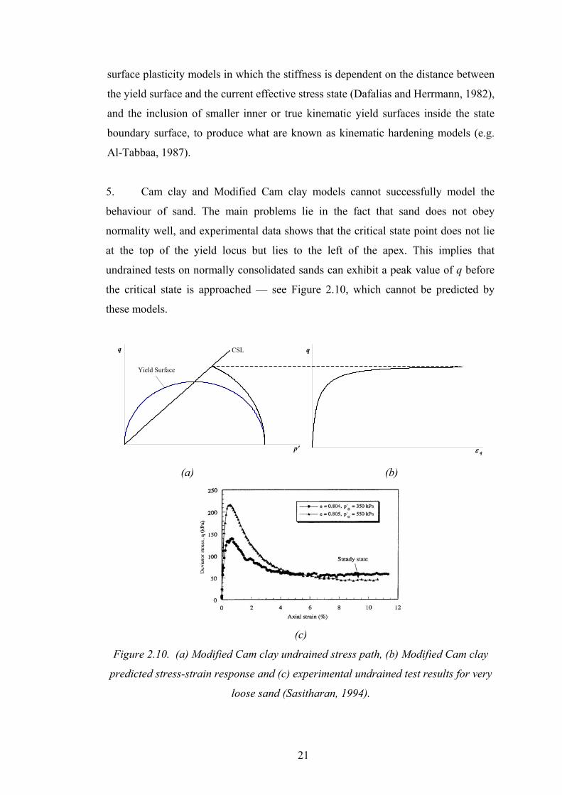
5. Cam clay and Modified Cam clay models cannot successfully model the

behaviour of sand. The main problems lie in the fact that sand does not obey

normality well, and experimental data shows that the critical state point does not lie

at the top of the yield locus but lies to the left of the apex. This implies that

undrained tests on normally consolidated sands can exhibit a peak value of q before

the critical state is approached — see Figure 2.10, which cannot be predicted by

these models.

p'

q

Yield Surface

CSL

ε q

q

(a) (b)

(c)

Figure 2.10. (a) Modified Cam clay undrained stress path, (b) Modified Cam clay

predicted stress-strain response and (c) experimental undrained test results for very

loose sand (Sasitharan, 1994).

21

6. The modelling of soils under cyclic loading is another deficiency in these

elasto-plastic models. The essential features of the Cam clay model are that, on

primary loading, large plastic strains occur, but on subsequent unload-reload cycles

within the yield surface, only purely elastic strains are produced. This is not suitable

for modelling the behaviour of soil under cyclic loading as, in reality, unload-reload

cycles result in the gradual accumulation of permanent strain and/or pore pressure,

and hysteretic behaviour occurs. The response of soil to undrained cyclic loading,

according to the Cam clay model, is shown in Figure 2.11 (Wood, 1990), whereas

the typical response of soil observed in cyclic loading is shown in Figure 2.12

(Wood, 1990).

Various models, such as the Bounding Surface model developed by Dafalias and

Herrmann (1982) and the ‘Bubble’ model by Al-Tabbaa (1987), can produce some

of the essential features of soil under cyclic loading.

7. Cam clay and Modified Cam clay do not take into account the effect of

time on soil deformation i.e. soil deforms at constant effective stress (known as

creep).

Figure 2.11. Modified Cam clay predictions of undrained cyclic loading: (a)

effective stress path, (b) stress-strain response and (c) pore pressure-strain response

(Wood, 1990).

22

Figure 2.12. Typical response of soil under cyclic loading: (a) effective stress path,

(b) stress-strain response and (c) pore pressure-strain response (Wood, 1990).

2.2.7 Advanced Models

Various more advanced models which are based on the Cam clay and the Modified

Cam clay models have been proposed in the past to make better predictions of soil

behaviour. These models are briefly described in this section.

The yield surfaces and plastic potentials of real soils appear to exhibit a variety of

shapes and it is therefore desirable to adopt an expression which has flexibility.

Lagioia et al. (1996) developed mathematical expressions for the plastic potential

and yield surface, which not only eliminate the limitations of the original Cam clay

model, but also produce a wide range of shapes. Some of the shapes currently found

to exist empirically in the literature can be reproduced by means of an appropriate

choice of parameters. The stress-dilatancy relation proposed by Lagioia et al. (1996)

is:

23

( ) 21

d MMd

ppp

q

ccε

ηε η

1

= −

+ (2.31)

where c1 and c2 are material constants.

A family of yield surfaces was also developed by Yu (1998), which is suitable for

both clay and sand. This model, Clay And Sand Model (CASM), requires two

additional parameters to describe the yield surface. One of these parameters is used

to specify the shape of the yield surface and the other is to control the position of the

critical state on the yield surface (i.e. to control the separation of the isotropic normal

and critical state lines in e-log p' space). One of the main features of this model is

that the critical state in this model does not necessarily occur at the maximum

deviatoric stress on the yield surface as opposed to the Original and Modified Cam

clay models (see Section 2.2.6). This is observed experimentally for sands (e.g.

Coop, 1990). However, the use of Rowe’s stress-dilatancy relationship as the flow

rule leads to non-associated flow at low stress ratios which is not observed

experimentally (McDowell, 2002).

A family of yield loci was derived by McDowell (2000) based on the new work

equation proposed by McDowell and Bolton (1998). The new work equation is given

as:

fracfricpq WWpq δδδεδε +=+ ' (2.32)

The left hand side is the plastic work done by the boundary stresses, which is

assumed to be dissipated in friction caused by particle arrangement and in the

fracture of particles. The first and second terms on the right are the energy dissipated

in friction and in fracture respectively. If the ratio of the work dissipated in fracture

to the work dissipated in friction is assumed to be a simple function of stress ratio,

McDowell (2000) showed that a simple stress-dilatancy relation could be developed

with the equation:

24

1 1p a app a

q

dd

ε ηε η

+ +Μ −= (2.33)

where η = q/p', M is the critical state dissipation constant, and a is constant.

This stress-dilatancy rule generates a yield surface whose equation is:

( )1

1'' 1 ln'

acpq p a

p

+ = Μ +

(2.34)

where p'c is the isotropic pre-consolidation pressure.

By changing the parameter a, different shapes of yield loci can be obtained,

consistent with those commonly encountered for isotropically consolidated clays and

sands.

2.2.8 Cyclic Loading Models

Various models have been developed for cyclic loading. Iwan (1967) and Mróz

(1967) independently formulated the first kinematic hardening model for metals

which was later applied to soils by Prévost (1977, 1978). Mróz et al. (1979)

described a two-surface kinematic hardening model which has a kinematic yield

surface inside the consolidation surface. If the current stress state reaches the yield

surface, plastic deformations occur and the yield surface translates. Hashiguchi

(1985) described a model which is similar to the model described by Mróz et al.

(1979) and introduced an extra surface in order to obtain a smooth stress-strain curve

beyond yield. Hashiguchi (1993) also describes in detail how the kinematic

hardening concept may be applied to generate multi-surface and infinite surface

models.

Dafalias and Herrman (1982) the bounding surface model, which can produce an

accumulation of permanent strain with increasing number of cycles. This model is

25

based on the concept of Critical State Soil Mechanics. The yield surface of a

conventional elastic-plastic model is now termed the bounding surface; it is no

longer the boundary between elastic and plastic deformations. In this model, the

sudden change of stiffness associated with the passage of the stress state through a

yield surface is eliminated by making the stiffness fall steadily from the high

(elastic) value at a point in the interior of the bounding surface to the low (plastic)

value when stress state reaches the bounding surface. For a stress state A, an image

point on the bounding surface B is defined by a radial mapping rule from a

projection origin O (Figure 2.13). The stiffness is made to be a function of the

distance between the stress state and the image stress. The salient feature of the

bounding surface model is the occurrence of plastic deformation for stress states

inside the bounding surface, and the possibility of having a very flexible variation of

the plastic modulus with changing stress states.

σ

O

Bounding surface

Figure 2.13. Schematic diagram showing the

Another simple way of modelling cyclic loading b

soil model is by reducing the size of the yield su

unloading. This model, developed by Carter et al.

the yield surface remains unchanged but that its size

manner by the elastic unloading. This model is ba

model with one important modification: the size of

unloading, with the left apex always passing through

allows for accumulating plastic strain and pore pres

26

B

A

Loading Surface

bounding surface concept.

ehaviour using the critical state

rface in an isotropic manner on

(1982) assumes that the form of

has been reduced in an isotropic

sed on the Modified Cam clay

the yield surface shrinks during

the origin. The resulting model

sure but not for hysteresis. Only

one additional parameter is needed which can be determined by performing cyclic

triaxial tests under undrained conditions.

Pender (1982) proposed a cyclic loading model based on the Critical State Soil

Mechanics framework. The initial version of the model predicted a rapid

accumulation of strains with increasing number of cycles. This is contrary to

observed behaviour where a state of equilibrium will be reached if the stress level is

less than a critical stress level (Sangrey et al., 1969; Brown, Lashine and Hyde,

1975). To remedy this defect Pender (1982) modified the hardening function of the

model by introducing a cyclic hardening index that depends on the number of cycles.

This allows the stiffness to increase with number of cycles, so that the material gets

progressively stiffer. However this does not solve the dilemma of how to model

monotonic behaviour following a history of cyclic loading.

Ghaboussi et al. (1982) proposed a cyclic model for sand using isotropic and

kinematic hardening for the yield surface. A hardening modulus is assumed and

volumetric strain is computed based on a semi-empirical relationship and the plastic

deviatoric strain is computed from a non-associated flow rule. The model

underestimates the amount of accumulated irreversible shear strain whereas the

predicted volumetric strain is reasonably accurate.

Nova (1982) described a model, which is suitable for both granular material and

clay. The model uses two different flow rules for high stress ratio and low stress ratio

such that non-associated flow is observed at high stress ratios whereas associated

flow is observed at low stress ratios. A smooth transition is ensured between these

flow rules. To model cyclic loading, Nova (1982) suggested that during unloading

the bulk and shear compliance varied and at the start of reloading the bulk and shear

compliance were restored to the initial values.

Al-Tabbaa (1987) developed a two-surface kinematic hardening model, known as

the ‘Bubble’ model, based on the Modified Cam clay model, which enables more

accurate predictions of the stress-strain behaviour of kaolin in overconsolidated

states. This two-surface bubble model is similar to the models described by Mróz et

al. (1979) and Hashiguchi (1985). A small inner true yield surface, which bounds a

27

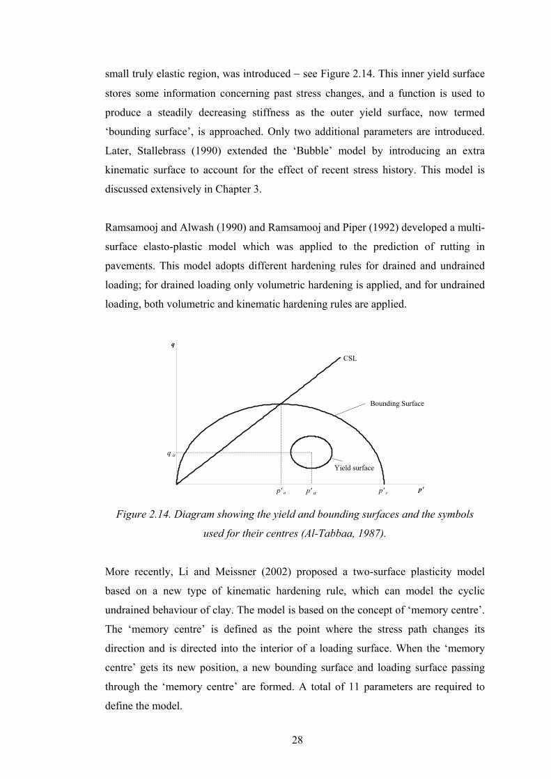
small truly elastic region, was introduced − see Figure 2.14. This inner yield surface

stores some information concerning past stress changes, and a function is used to

produce a steadily decreasing stiffness as the outer yield surface, now termed

‘bounding surface’, is approached. Only two additional parameters are introduced.

Later, Stallebrass (1990) extended the ‘Bubble’ model by introducing an extra

kinematic surface to account for the effect of recent stress history. This model is

discussed extensively in Chapter 3.

Ramsamooj and Alwash (1990) and Ramsamooj and Piper (1992) developed a multi-

surface elasto-plastic model which was applied to the prediction of rutting in

pavements. This model adopts different hardening rules for drained and undrained

loading; for drained loading only volumetric hardening is applied, and for undrained

loading, both volumetric and kinematic hardening rules are applied.

p'

q

CSL

p' c

Yield surface

Bounding Surface

p' o

q α

p' α Figure 2.14. Diagram showing the yield and bounding surfaces and the symbols

used for their centres (Al-Tabbaa, 1987).

More recently, Li and Meissner (2002) proposed a two-surface plasticity model

based on a new type of kinematic hardening rule, which can model the cyclic

undrained behaviour of clay. The model is based on the concept of ‘memory centre’.

The ‘memory centre’ is defined as the point where the stress path changes its

direction and is directed into the interior of a loading surface. When the ‘memory

centre’ gets its new position, a new bounding surface and loading surface passing

through the ‘memory centre’ are formed. A total of 11 parameters are required to

define the model.

28

2.2.9 Earth Pressure Coefficient at Rest

One-dimensional Loading

The prediction of the in-situ stress state in soil is of major importance in geotechnical

problems. Vertical stresses can be determined easily, but the determination of

horizontal stresses are more difficult. Many soils have a one-dimensional stress

history and in the analysis of any pavement subgrade, it will be necessary to consider

the stress history. This section therefore reviews literature on the one-dimensional

history of soils.

The ratio of the horizontal to vertical effective stresses in soil is called the coefficient

of earth pressure at rest, K0:

''h

0v

K σσ

= (2.35)

The value of K0 during one-dimensional normal compression, K0,nc, is known

empirically to be constant for a given soil. Numerous relationships between K0,nc and

angle of shearing resistance, φ', have been proposed over the past based on

experimental data. The most widely used is that proposed by Jâky (1944):

,2 1 sin1 sin '3 1 sin0 ncK '

'φφφ

− = + +

(2.36)

This equation is approximated to:

, 1 sin '0 ncK φ= − (2.37)

For clays, it is found that the value of φ' in equation 2.37 is the critical state angle of

friction, φ'crit. For sand, the value of φ' in equation 2.37 is less certain. According to

Wood (1990), for sand the value of K0,nc will depend on the initial structure of the

sand, and is therefore likely to depend on the maximum angle of shearing resistance

29

(Wood, 1990). However, for a sand which has yielded and is deforming plastically

under one-dimensional normal compression (i.e. the state lies on the state boundary

surface), it would be expected that the initial structure will have been eliminated, so

that the value of φ' in equation 2.37 will be φ'crit as for clay.

Brooker and Ireland (1965) proposed a modified form of Jâky’s equation for

cohesive soil:

0.95 sin '0 ncK φ= −, (2.38)

Bolton (1991b) suggested a relationship for sand:

( )( ),

1 sin ' 11.5

1 sin ' 11.5c

0 ncc

Kφ

φ

− −=

+ −

o

o (2.39)

Simpson (1992) proposed a relationship for K0,nc based on the ‘BRICK’ model:

,2 sin '2 sin '0 ncK φ

φ−

=+

(2.40)

One-dimensional Unloading

The effective horizontal stresses reduce more slowly than vertical effective stresses

during one-dimensional unloading. Therefore the K0 value for overconsolidated clay

increases with overconsolidation ratio (OCR). Wroth (1975) derived an expression

for K0 on unloading for lightly overconsolidated soil based on the assumption that on

unloading the soil is linear elastic.

(,'OCR OCR 1

1 '0 0 ncK K )µµ

= ⋅ − −−

(2.41)

This relationship is only suitable for soil with OCR of not more than four where the

unloading line in q − p' space is approximately linear. Numerous researchers have

30

proposed empirical relationships for K0 on unloading which can fit experimental data

well. A simple expression was given by Schmidt (1966) for clays for K0 on

unloading as a function of K0,nc and OCR:

[ ], OCR0 u 0 ncK K α= , (2.42)

where:

α = sin 1.2φ'crit (2.43)

Meyerhof (1976) suggested that α = 0.5 is suitable for most soils for most practical

purposes. Based on the study of experimental data on 170 different soils, Mayne &

Kulhawy (1982) suggested that:

α = sin φ'crit (2.44)

Al-Tabbaa (1987) performed oedometer tests on Speswhite kaolin and found that α

= 0.464, which agrees well with equation 2.43 with φ'crit = 23°.

Pruska (1973) proposed an expression for the variation of K0 with OCR:

( )OCR

1 1 OCa

0,ua

KK

K⋅

=− ⋅ − R

(2.45)

where Ka is the Rankine active earth pressure coefficient:

1 sin '1 sin 'aK φ

φ−

=+

(2.46)

One-dimensional Reloading

Very little data has been published for one-dimensional reloading. Based on the data

available, Mayne & Kulhawy (1982) proposed a relationship for K0 during reloading,

31

K0,r which will reduce to equation 2.37 for normally consolidated soils, i.e. OCRmax =

OCR = 1, where OCR is the overconsolidation ratio. Equation 2.47 suggests that K0,r

would not join the virgin curve at OCR = 1:

, 1 sin 'max max

OCR 3 OCR1 sin ' 1OCR 4 OCR0 rK φφ −

= − + −

(2.47)

Schmidt (1983) suggested that for reloading, K0,r would return to K0,nc at OCR = 1

and proposed an expression for K0,r:

( )( ), maxmax

1 sin ' OCR OCR OCR 1 OCROCR 10 rK α

maxφ−

= − + −−

(2.48)

These equations suggest that K0,r varies linearly with OCR. Al-Tabbaa (1987) found

that Schmidt’s equation 2.48 fitted her data exactly with α = 0.464 for Speswhite

kaolin.

Since the stresses which occur during one-dimensional history will be related to the

strains via a flow rule, the above data can be used to test the validity of any new

model which may be developed for clays. This is discussed in Chapters 3 and 4.

2.3 PAVEMENT ENGINEERING

2.3.1 Pavement Types and Failure Modes

The purpose of a pavement is to support the loads induced by traffic and to distribute

these loads safely to the foundation. There are several different types of pavement

but this project is concerned specifically with lightly trafficked (or low volume)

flexible pavements, and hence other types of pavement are not in the scope of this

research. Behrens (1999) defines low volume roads as those in a rural environment

that enable automobile operation and account for less than 500 vehicles per day.

Since lightly trafficked roads require relatively thin layers of bituminous material

32

compared with motorways, the pavement foundation properties assume greater

significance since they are more highly stressed. The main objective of this research

is the application of the principles of soil mechanics to the pavement foundation.

Figure 2.15 shows a typical cross-section of a flexible pavement. This pavement

comprises a number of bituminous layers placed over road base (unbound or bound

material) over crushed stone or a similar unbound sub-base material placed on the

natural subgrade. This pavement is referred to as ‘flexible’ because the bituminous

materials are capable of flexing slightly under traffic loading. For thinly surfaced

pavements, the road base is often unbound material and not formally part of the

foundation. However, for the purposes of this work it can be regarded as part of the

foundation.

The pavement foundation is defined as the granular layer or layers placed over the

subgrade and the subgrade itself — see Figure 2.15. The reason for considering all

the unbound granular material is that the principles of soil mechanics apply to the

sub-base, capping and subgrade. These principles have not been effectively applied

in pavement engineering. Capping is a relatively cheap material placed between the

subgrade and the sub-base to protect weak subgrades.

Moving wheel load

Subgrade (Clay)

Surfacing (bituminous material)

Sub-base (granular material)

Road base

Foundation

Figure 2.15. Cross-section of pavement.

In order to design a flexible pavement, the failure mechanisms must be adequately

understood. Pavements do not fail suddenly but gradually deteriorate with time to a

terminal level, which may be defined as failure. When a vehicle trafficks a road, it

induces a stress pulse in the subgrade and granular layer. Figure 2.16 shows the

33

stresses in a pavement under a wheel load (Lekarp et al., 2000). This stress pulse

causes strain and this strain can be divided into two parts: recoverable and permanent

strain — see Figure 2.17.

Figure 2.16. Stress pulse induced by a wheel load in a pavement foundation (Lekarp

et al., 2000).

q

Permanent strain

Resilient strain

Figure 2.17. Diagram showing recoverable and permanen

resilient modulus.

The two main structural failure mechanisms for flexible

deformation (rutting) and fatigue cracking. These two fa

Figure 2.18. Rutting is the result of an accumulation of i

various pavement layers. In the U.K., a pavement is a

‘critical’ conditions when the rut depth reaches 10mm and

34

Resilientmodulus

εa

t strains and definition of

pavements are permanent

ilure modes are shown in

rrecoverable strains in the

ssumed to have reached

failure is assumed to have

occurred when 20mm rut depth is reached. For a lightly trafficked pavement,

subgrade and granular layer contribute most to rutting of a pavement. Fatigue

cracking has been defined as the phenomenon of fracture under repeated or

fluctuating stress having a maximum value generally less than the tensile strength of

the material (Ashby and Jones, 1980). In the U.K., a pavement is usually assumed to

have reached ‘critical’ conditions at the onset of fatigue cracking in the wheel path.

Failure conditions have been reached when there is evidence of extensive cracking in

the wheel path.

Figure 2.18. Diagrams showing the two types of failure mechanisms in pavements.

2.3.2 Resilient Deformation Models

The concept of resilient behaviour of pavements was introduced by Hveem &

Carmany (1948) and Hveem (1955). In the 1950s, Seed et al. (1955) at the

University of California at Berkeley followed the lead established by Hveem, who

had developed the repeated load test. They introduced the term ‘modulus of

resilience’, which they later changed to ‘resilient modulus’ (Seed et al., 1962) — see

Figure 2.17. The definition of resilient modulus is the ratio of the repeated deviator

stress to the recoverable (resilient) axial strain in the triaxial test (Seed et al., 1962).

This concept has gained recognition by the pavement community as a good property

to describe the resilient behaviour of granular materials and subgrade soils.

35

The resilient response of the soil plays an important role in pavement design, as this

is the factor, which determines the thickness and stiffness of higher layers so that

adequate load spreading takes place. During pavement construction, if the resilient

deformations are too high, the paving plant will not be able to satisfactorily compact

the bituminous layers of the pavement. The resilient response of unbound aggregates

has been found to be influenced by many factors. An extensive literature review on

the effect of different factors affecting the resilient response of unbound aggregates

was performed by Lekarp et al. (2000), who describe the available modelling

techniques. The factors affecting the resilient behaviour of unbound aggregates are

stress level, density, grading, fines content, maximum grain size, moisture content,

stress history, number of load cycles, aggregate type and particle shape, load

duration and sequence. Among these, Lekarp et al. (2000) found that the effect of

stress level on the resilient behaviour is the most significant factor. Resilient

modulus increases greatly with confining pressure, and decreases with increasing

deviator stress q.

The model most widely used for resilient deformations of unbound granular

materials is the so-called K-θ model, which expresses the resilient modulus, Mr as a

function of the sum of principal total stresses, θ:

2

1k

r kM θ= (2.49)

where k1 and k2 are the constants and θ = 3pmax and pmax is the maximum mean stress

during the load cycle. This model was developed by Hicks et al. (1971) based on

repeated load conventional triaxial tests (constant radial stress σr) performed on two

types of aggregate, namely crushed gravel and crushed rock.

Later Boyce (1980) developed a non-linear purely elastic model, G-K model based

on the theorem of reciprocity (the proof of which was given by Boyce (1980)):

pq

qp

∂

∂=

∂

∂ εε (2.50)

36

In this model Boyce expressed the bulk modulus K and shear modulus G as a

function of mean normal stress p to a power less than one:

( )11

tK K p −= (2.51)

( )1

1tG G p −= (2.52)

where K1, G1 and t are material constants. This model is similar to the K-θ model

described above.

Since equations 2.51 and 2.52 do not satisfy the reciprocity theorem (equation 2.50),

Boyce suggested a more complicated approach which satisfies this. The resilient

volumetric strain, εpr and the resilient shear strain εqr proposed by Boyce have the

following expressions:

2

21

1 1tpr

qpK p

ε

= −

ω (2.53)

1

13

tqr

qpG p

ε = (2.54)

where

( ) 1 11 / 6t K Gω = − (2.55)

This G-K model contains only three parameters, K1, G1, and t, to describe the

resilient deformation of the material. The constant K1 is the bulk modulus when the

mean normal stress is 1kPa and the deviatoric stress is zero, and G1 is the shear

modulus when the mean normal stress is 1kPa. The parameter t is a measure of stress

dependency, and varies between 0 and 1. For t = 1, a linear elastic relationship is

obtained. This model was later modified by others such as Sweere (1990) to improve

predictive capability.

37

In order to incorporate the resilient modulus, Mr, into the pavement design methods,

some empirical correlations based on California Bearing Ratio (CBR) are widely

used, such as:

CBRM r 10= [MPa] (2.56)

proposed by Heukelom & Klomp (1962), and:

[MPa] (2.57) 64.06.17 CBRM r =

proposed by Powell et al. (1984). CBR is the average ratio, expressed as a

percentage, of the loads required to penetrate a given material and a standard

material by 2.5mm and 5mm. The CBR test is briefly described in Section 2.3.5.

Brown et al. (1987) demonstrated that the resilient modulus is stress dependent and

non-linear and checked the validity of equations 2.56 and 2.57; the results are shown

in Figure 2.19. It was found that the resilient modulus is not a simple function of

CBR; it depends on stress level and material type.

Figure 2.19. Relationships between resilient modulus and CBR (Brown et al., 1987).

38

2.3.3 Permanent Deformation Models

Fewer permanent deformation models have been proposed compared to those for

resilient deformation because permanent deformation tests are time consuming and

destructive. Models for permanent deformation are based on repeated load triaxial

tests with a large number of cycles and the permanent strain is related to the number

of load applications. Barksdale (1972) performed a series of repeated load triaxial

tests with 105 cycles on different granular materials, and found that the accumulation

of permanent axial strain was proportional to the logarithm of number of load cycles.

Barksdale (1972) suggested the following expression:

1 2 logap a a Nε = + (2.58)

where εap = permanent axial strain, N = number of load cycles and, a1 and a2 are

constants for a given stress level.

Later, Sweere (1990) showed that, after applying 106 cycles, a log-log approach is

more appropriate for large numbers of cycles:

1 2log logap a a Nε = + (2.59)

Other approaches relate the permanent strain to the length of the stress path and

stress ratio such as Pappin (1979) and Lekarp et al. (1998).

A full range of repeated load triaxial tests was carried out by Pappin (1979) on a

well-graded crushed limestone with a maximum particle size of 38mm, which is

commonly used in pavements in the U.K. The objective of these tests was to

investigate the permanent strain behaviour and to formulate a predictive model. In

each test an attempt was made to apply at least 100,000 cycles of load at a frequency

of 1Hz. From these results Pappin derived an expression for permanent shear strain:

( )2.8 2.8

4

max

2 103qpqb L pε − = × × ×

(2.60)

39

where εqp is permanent shear strain in %, b is the shape factor, which is calculated

for different numbers of cycles, and L is the stress path length in kPa.

Lekarp et al. (1998) used the repeated load triaxial equipment and hollow cylinder

apparatus at Nottingham to test five different granular materials, which are

commonly used as sub-base materials in pavement structures. The objective was to

study the development of permanent strain with increasing number of load cycles

and as a function of stress level. A relationship that takes account of stress path

length and stress level was proposed by Lekarp et al. (1998) for permanent axial

strain:

( ) 2

1max

aap ref

r

N qaL p p

ε =

(2.61)

where εa,p(Nref) is the accumulated permanent axial strain at a given number of

cycles, L is the length of the stress path in kPa, a1 and a2 are regression parameters

and pr is a reference stress, taken to be 1kPa. Lekarp et al. (1998) found that the

growth of permanent strain would eventually reach an equilibrium condition, at

which the rate of growth of permanent strain was zero, if the stress ratio was low.

However, at high stress ratios the accumulation of permanent strain was more

progressive, indicating that a threshold stress ratio must exist above which

accumulation of permanent strain will cause progressive failure. This threshold stress

ratio is called the shakedown limit.

2.3.4 Stress History of a Pavement

The response of an element of soil to applied load depends crucially on its stress

history and current stress state. The soil beneath a pavement may be in its natural

undisturbed state or be remoulded depending on whether the section of pavement is

in a ‘cut’ or ‘fill’ area (Brown, 1996), and these two situations have to be treated

separately. Brown (1996) illustrated the typical stress history for an element in a

‘cut’ condition and in a ‘fill’ condition. For the cut or undisturbed condition, the

40

typical stress history is shown in Figure 2.20 (Brown, 1996). The stress path from

point O to point C and to point A in Figure 2.20 represents the natural stress history

of soil due to one-dimensional compression and subsequent unloading due to

erosion. This historical sequence generates an overconsolidated soil. Subsequent

pavement construction operations will bring the soil to the final state P. The

construction operation of a pavement involves three processes, which will influence

the stress state of soil. These are:

1. Removal of overburden during earthworks construction

2. Lowering of the water table

3. Addition of overburden due to the pavement construction.

Figure 2.21 (Brown, 1996) shows the effects of construction operations on stress

conditions in a ‘cut’ condition. The path AB is due to the removal of overburden,

and as time passes, pore pressure will reach equilibrium as the effective stress moves

from B to P'. The path P'D results from lowering the water table. Construction of the

pavement will take place before point D is reached and therefore the increase of

overburden due to construction will cause the effective stress to move from E to F.

After the dissipation of pore pressure, the effective stress will move towards

equilibrium at P. In reality, the actual stress path is likely to be represented by the

curve BGEP due to the time needed for the dissipation of pore pressure.

For soil which is cut, transported and compacted as fill in an embankment, the

effective stress regime is rather different and less well understood. Brown (1996)

suggested a possible stress regime for construction in the ‘fill’ condition, shown in

Figure 2.22. The soil is first brought to failure in an undrained condition due to the

scraper operation – represented by AB in Figure 2.22. The stress state will then move

to Q or Q', depending on the environment and weather conditions. The effective

stress state will move to Q if conditions are dry and the soil is placed above the water

table at which suctions will be high and tend to increase the effective stress. If

conditions are wet, the soil will move to a lower effective stress state such as Q'. The

stress state at Q' will move to Q after equilibrium conditions have been reached. The

net effect on soil due to the 'fill' condition is then a reduced overconsolidation ratio

after excavation, transportation and compaction as fill.

41

Figure 2.20. Typical stress history in a ‘cut’ condition (Brown, 1996).

Figure 2.21. Effect of construction operations (Brown, 1996).

Figure 2.22. Stress history in a ‘fill’ condition (Brown, 1996).

42

2.3.5 Current UK Flexible Pavement Design Methods

The current UK practice of flexible pavement design is based on the Design Manual

of Roads and Bridges (DMRB), Volume 7 (Highways Agency, 1994). This method

was established by considering the performance of a number of experimental roads

and is essentially empirical. The subgrade of a pavement is characterised by the

California Bearing Ratio (CBR) concept developed in the US by the California

Division of Highways in 1938. The CBR test involves the insertion of a plunger into

the soil sample which is constrained within a small mould; the test procedure can be

found in BS1377:1990 Part 4 (British Standards Institution, 1990). The load and the

penetration are recorded while the plunger penetrates the sample. The loads at a

penetration of 2.5mm and 5mm are compared with the result for a standard sample

and the ratio expressed as a percentage is the CBR of the soil. The CBR of a

pavement subgrade determines the thickness of the sub-base required using the

empirical charts in DMRB Volume 7. This empirical design method provides no

confidence when different types of material are used.

Some other design methods based on linear elastic theory were also proposed; the

Shell design method (Shell, 1978) is the most common procedure using this theory.

In this method, the pavement structure is represented by a three-layer system

comprising an asphalt layer over a granular sub-base over the subgrade. This system

is analysed using a multi-layered elastic theory with a program such as BISAR. The

design criteria are to limit the maximum tensile strain at the bottom of the asphalt

layer so that fatigue cracking of the asphalt layer will not occur, whilst the rutting of

a pavement is related to the maximum compressive strain at the top of the subgrade.

The non-linear properties of soil are not taken into account by this method. Brown

and Dawson (1992) proposed a design method for asphalt pavements, which allows

for the non-linear resilient behaviour of soils by using an equivalent resilient

modulus. The design process is divided into two stages. The first involves the

determination of the thickness of granular material required to protect the subgrade

from being excessively stressed during the construction stage, and the second stage

involves the design of the thickness of the asphaltic material required to prevent

rutting and fatigue cracking when the pavement is opened to traffic. The thickness of

43

the granular material is chosen such that the deviatoric stress at the top of the

subgrade does not exceed a certain value.

Brown and Brunton (1986) proposed a simplified approach to the design of flexible

pavements, which assumes a standard 200mm layer of granular material with a

resilient modulus of 100MPa. The subgrade is characterised by a single resilient

modulus of value between 20 and 100MPa, which in the absence of better

information, can be estimated from some empirical relationships between resilient

modulus and CBR as described in Section 2.3.2. The design process involves the

determination of an appropriate thickness of asphalt layer to ensure that the resilient

tensile strain at the bottom of the asphalt layer and the resilient compressive strain at

the top of the subgrade are below their maximum allowable values.

All of these design methods are either empirical or based on linear elastic theory,

with little or no input from conventional Critical State Soil Mechanics.

2.4 NUMERICAL MODELLING

2.4.1 Introduction

The theory of elasticity has been extensively applied to the analysis of layered

pavement systems. Various computer programs have been developed to analyse

pavements. The most widely used layered elastic program in pavement engineering

is BISAR, developed by Shell (Shell International Petroleum Company, 1978).

Pavement layers are assumed to be linear elastic. A constant value of Young’s

modulus E' and Poisson’s ratio µ', is assigned to each layer. The use of constant

values for E' and µ' is a simplification, made to allow the use of a relatively simple

computer program based on linear elastic theory. Linear elastic analysis can be used

with reasonable confidence for pavements where the main structural element is

formed by the asphalt layer (thick asphalt). However, for thinly surfaced (low

volume) or unsurfaced pavements the simplification to a linear elastic system is no

longer justified due to the fact that pavement foundations have markedly non-linear

44

and inelastic stress-strain relationships. This non-linearity and inelasticity must be

properly taken into account in theoretical analysis. To accommodate this non-

linearity, the granular layer and soil can be subdivided into sub-layers. Stress-

dependency of the stiffness can then be taken into account by assigning a higher

stiffness to the deeper sub-layers. The problem of obtaining a correct stiffness for

each sub-layer remains. To accommodate the accumulation of permanent

deformation, however, any kind of layered elastic approach is useless. It has to be

used in conjunction with other empirical relationships which relate the permanent

deformation to stresses computed from layered elastic analysis, and the number of

load applications (Barksdale, 1972).

Most of the pavement analysis accommodating non-linear behaviour, has used the

finite element approach. Several finite element packages specially developed for the

pavement problem such as SENOL (Brown and Pappin, 1981) and FENLAP

(Almeida, 1993) have been developed at the University of Nottingham. These

programs use empirical stress-strain relationships to model the material behaviour.

2.4.2 Basic Finite Element Concepts

The basic steps involved in the formulation and application of the finite element

method are:

• Step 1: Element Discretization

This step involves subdividing the structure into a number of small regions, termed

finite elements. These elements have nodes or nodal points, which are the

intersections of the sides of the elements.

• Step 2: Select Approximate Models or Functions

In this step, the primary unknown quantity must be selected such as displacement or

stress. This variable is expressed in terms of nodal values by mathematical functions

such as polynomials.

45

• Step 3: Define Stress-strain Relationships

A constitutive relationship which describes the stress-strain behaviour is defined:

{ } [ ]{ }εσ ∆=∆ D (2.62)

where [D] is the constitutive matrix relating the change in stress to the change in

strain.

• Step 4: Derive Element Equations

Energy methods and residual methods are the two methods commonly used in the

derivation of element equations (Desai, 1979). The element equations are

commonly expressed as:

[ ]{ } { }EEE RdK ∆=∆ (2.63)

where [KE] is the element stiffness matrix, {∆dE}, is the vector of increment

element nodal displacements and {∆RE} is the vector of element incremental

nodal forces.

• Step 5: Assemble element equations to obtain global equations and introduce

boundary conditions.

In this step, element equations are combined to form global equations for the

entire structure, which define approximately the behaviour of the structure as a

whole. The global equations are expressed as:

[ ]{ } { }GGG RdK ∆=∆ (2.64)

where [KG] is the global stiffness matrix, {∆dG}, is the vector of all incremental

nodal displacements and {∆RG} is the vector of all incremental nodal forces.

Boundary conditions are the physical constraints or supports that exist so that the

structure can stand in space uniquely. These conditions are known values.

46

• Step 6: Solve for the Primary Unknowns

Equation 2.64 is a set of simultaneous equations. In this step, these simultaneous

equations are solved to obtain {∆dG} using Gaussian elimination or iterative

methods.

• Step 7: Solve for Derived or Secondary Quantities

Once the primary quantities are obtained, secondary quantities such as stresses

and strains can be evaluated.

If the material is linear elastic, the constitutive matrix [D] is constant. However, the

behaviour of soil is highly non-linear, and if the soil is assumed to be non-linear

elastic or elasto-plastic the constitutive matrix [D] is no longer constant but varies

with stress or strain: it changes during a finite element analysis. The finite element

method can be adapted to deal with non-linear constitutive relationships by applying

the boundary conditions incrementally. This causes the governing finite element

equations to be reduced to incremental form:

[ ] { } { }iG

inG

iG RdK ∆=∆ (2.65)

where [KG]i is the incremental global system stiffness matrix, {∆d}inG is the vector

of incremental nodal displacements, {∆RG}i is the vector of incremental nodal forces

and i is the increment number. Due to the non-linear constitutive relationships, the

incremental global stiffness matrix [KG]i varies during an increment, and hence the

solution of equation 2.64 is not straightforward. There are three different methods

used to solve these equations: (1) Tangent stiffness method (2) Visco-plastic method

and (3) Modified Newton-Raphson (MNR) method. In principle, if the number of

increments applied is sufficiently large, all methods should give similar results.

However, an increase in the number of increments will increase the computational

time. Hence the method used in non-linear finite element analysis plays an important

role, as it can influence the amount of computational effort required to obtain the

results and the accuracy of the results (Potts & Zdravković, 1999).

47

The tangent stiffness method is the simplest and most widely used method in

engineering practice. This is the method used in the finite element program CRISP

(Britto and Gunn, 1987). In this method, the total applied load is divided into a small

number of increments and each increment is applied individually. During each

increment, the stiffness properties appropriate for the current stress levels are used in

the calculations. Provided the increments are small, the material behaviour may be

assumed to be linear during the load increment. If only a few increments are used,

this method produces a solution which tends to drift away from the exact solution –

see Figure 2.23.

Figure 2.23. Tangent stiffness method (Potts & Zdravković, 1999).

2.4.3 Critical State Program (CRISP)

CRISP (Critical State Program) was developed by research workers in Cambridge

University (Britto and Gunn, 1987). This is a finite element program which is able to

perform drained, undrained and time dependent analysis of static problems under

monotonic loading or unloading conditions. It is not suitable for cyclic loading in its

currently commercially available form. Plane strain, axisymmetric and three-

dimensional analysis can be carried out. Various constitutive models, from linear

elastic models to advanced critical state models, are available in CRISP. However,

the constitutive models currently available in CRISP are not suitable for analysing

48

partially saturated soils. Different types of finite element are available such as linear

strain triangle and cubic strain triangle.

Modifications made to CRISP

In order to simulate the pavement subgrade under cyclic loading, thousands of cycles

have to be applied. Without modification to the program, it is very tedious and time

consuming to generate large numbers of cycles. A computer program, which is able

to generate large numbers of cycles automatically, was written by the CRISP

Technical Support for the purpose of this project. This greatly reduces the amount of

time required to generate a large number of load cycles. This program was also

modified by CRISP Technical Support so that a large number of cycles of multiple

stress blocks can be applied automatically. This is important, because it makes it

possible to calculate the stress distribution at the top of the subgrade clay in a three-

layer pavement due to an applied wheel load. This stress distribution can be

approximated by rectangular stress blocks applied repeatedly to the surface of the

clay subgrade. This was found to be particularly helpful, because if a three-layer

pavement is analysed directly in CRISP, and the nodes at the interfaces between

layers are common to each of the two layers at an interface, then each time the

pavement is unloaded, the upper elastic layers pull the subgrade soil into tension.

Thus, the use of stress blocks applied to the clay directly eliminates this problem,

with the assumption that the granular and bituminous layers will settle to follow the

surface of the clay in the long term.

2.5 SUMMARY

The most commonly used type of analysis in pavement engineering makes use of

multi-layered linear elastic theory. This requires the provision of a constant elastic

modulus and a Poisson’s ratio for each pavement layer including granular material

and clay. In conditions where the asphalt layer is relatively thick and hence the

pavement foundation is relatively insignificant due to the low stresses induced in this

49

layer, such analysis can give reasonable results. However, when the stresses in the

foundation layers are high such as in unsurfaced and thinly surfaced pavements, the

non-linear and inelastic properties become crucial and elastic theory will not be able

to predict correctly the behaviour of these types of pavements. It is clear that the

problem of analysis of pavements including soil is one that is still not completely

solved. This is particularly true for unsurfaced and thinly surfaced conditions, where

the rutting behaviour of the pavement under repeated loading will be largely

determined by the subgrade properties.

The majority of models developed specifically for pavement problems are

empirically based, and therefore provide no confidence when extrapolating to

different materials or different loading conditions. For the past decades, various

cyclic models for soil have been developed based on the CSSM concept, which have

been shown to be able to predict some of the essential features of soil under cyclic

loading. However, little effort has been put into applying these models to the

prediction of pavement response. The design methods developed for motorways are

generally adopted by the local authorities that are responsible for lightly trafficked

roads, which leads to uneconomical design standards. It is clear that there is an

urgent need to apply to pavement engineering the knowledge of soil mechanics that

has been accumulated through research, if economical design methods are to be

established, especially for thinly surfaced pavements where the behaviour of the

foundation plays a very important role.

50

3 PRELIMINARY STUDY – EVALUATION OF THE

TWO AND THREE-SURFACE KINEMATIC

HARDENING MODELS

3.1 INTRODUCTION

In the previous chapter, various models used in pavement engineering and soil

mechanics were briefly described. The existing models which can predict the

essential features of soil behaviour under cyclic loading are those based on the

kinematic hardening concept. In this chapter the formulation of the 3-SKH model is

briefly described, and the predictions of the two-surface model and the 3-SKH model

of the coefficient of earth pressure at rest and of soil behaviour under cyclic loading

in triaxial tests are evaluated. The main objective of this chapter is to establish

whether a kinematic hardening model is capable of predicting the response of a

typical three-layer pavement under cyclic loading. The suitability of both the two-

surface and the 3-SKH models for modelling the subgrade clay will be examined. In

this way, the advantages and disadvantages of the models can be determined and

necessary modifications to the models can be established in order to improve

predictive capability.

3.2 MODEL DESCRIPTION

The detailed derivation of the two-surface model (or the ‘Bubble’ model) and the 3-

SKH model are given in Al-Tabbaa (1987) and Stallebrass (1990) respectively.

These models are an extension of the Modified Cam clay model, but these models

are slightly different from the Modified Cam clay model in that the normal

compression lines and the swelling lines are assumed to be linear in ln v − ln p' space

with slopes λ* and κ* respectively (Butterfield, 1979), whereas in Modified Cam clay

these lines were assumed to be linear in v − ln p' space. In this section only the

formulation of the 3-SKH model is described as this is very similar to the

51

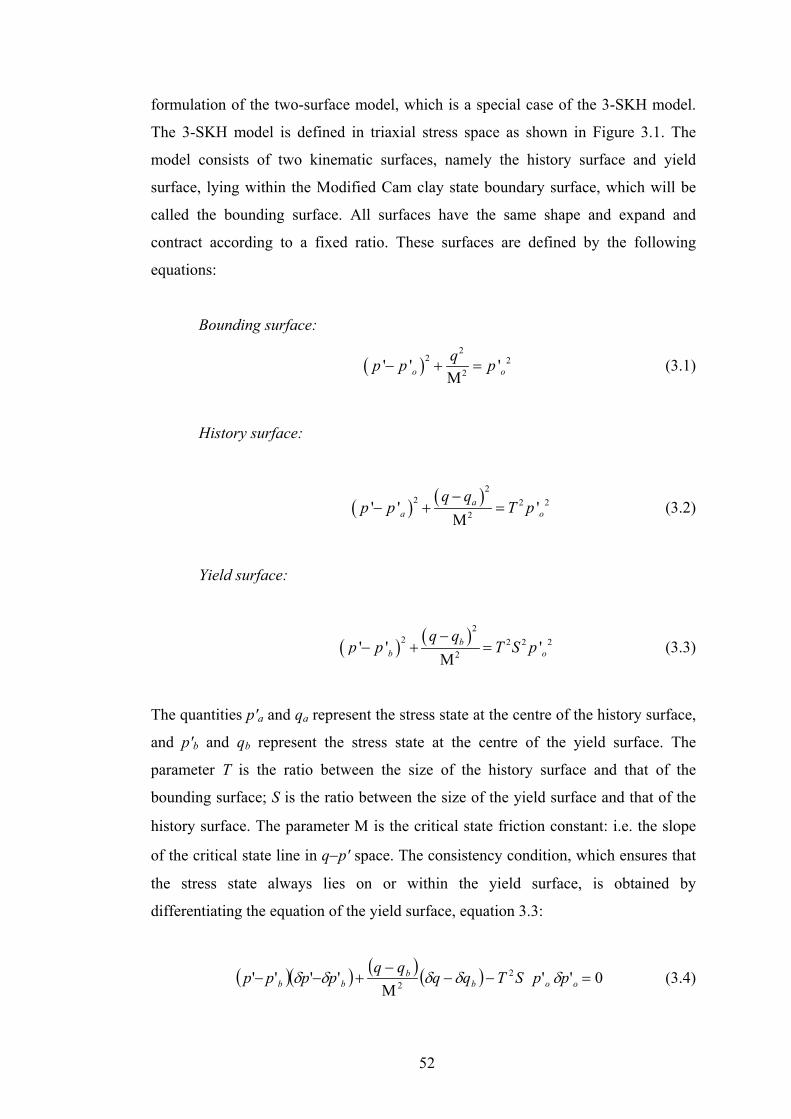
formulation of the two-surface model, which is a special case of the 3-SKH model.

The 3-SKH model is defined in triaxial stress space as shown in Figure 3.1. The

model consists of two kinematic surfaces, namely the history surface and yield

surface, lying within the Modified Cam clay state boundary surface, which will be

called the bounding surface. All surfaces have the same shape and expand and

contract according to a fixed ratio. These surfaces are defined by the following

equations:

Bounding surface:

( )2

2 22' ' '

Mo oqp p p− + = (3.1)

History surface:

( ) ( )22 2 2

2' ' 'M

aa

q qop p

−− + = T p (3.2)

Yield surface:

( ) ( )22 2 2 2

2' ' 'M

bb

q qop p T

−− + = S p (3.3)

The quantities p'a and qa represent the stress state at the centre of the history surface,

and p'b and qb represent the stress state at the centre of the yield surface. The

parameter T is the ratio between the size of the history surface and that of the

bounding surface; S is the ratio between the size of the yield surface and that of the

history surface. The parameter Μ is the critical state friction constant: i.e. the slope

of the critical state line in q−p' space. The consistency condition, which ensures that

the stress state always lies on or within the yield surface, is obtained by

differentiating the equation of the yield surface, equation 3.3:

( )( ) ( ) ( ) 0''M

'''' 22 =−−

−+−− oob

bbb ppSTqq

qqpppp δδδδδ (3.4)

52

The consistency equation for the history surface is:

( )( ) ( ) ( ) 0''M

'''' 22 =−−

−+−− ooa

aaa ppTqq

qqpppp δδδδδ (3.5)

q

2p'o

2Tp'o

2TSp'o

p'b p'a p'o

History surface

Yield surface

Bounding surface

qa qb

p'

Figure 3.1. Diagram showing the 3-SKH model in triaxial stress space (Stallebrass,

1990).

When the stress state of the soil lies within the yield surface, the deformations of the

soil are governed by isotropic elasticity:

* ' 00 1 3

epeq e

''

ppG

δε κδε q

δδ

=

(3.6)

where G'e is the elastic shear modulus: i.e. the shear modulus at very small strains

and κ* is the initial slope of the isotropic swelling line in ln v − ln p' space. The value

of G'e can be assumed to vary with p' and overconsolidation ratio, Ro according to

53

the relationship proposed by Viggiani and Atkinson (1995) (Stallebrass and Taylor,

1997):

( )' ' ' n me rG A p p R= o (3.7)

where p'r is a reference pressure equal to 1kPa, Ro is the overconsolidation ratio

(equal to p'c/p'), and m and n are material constants.

3.2.1 Translation Rule

The translation laws used to control the movement of the kinematic surfaces have the

same form as those used in the two-surface model developed by Mróz et al. (1979)

and Al-Tabbaa (1987). These translation laws follow a rule which states that the

centre of a surface should always move along a vector joining the current stress state

to its conjugate point on the next surface, as shown in Figure 3.2. The conjugate

point is defined as the point on the surface with the same outwards normal. When all

the surfaces are in contact, this model reduces to Modified Cam clay.

The conjugate point corresponding to the current stress state can be calculated using

the following equation:

' '' '

0

b

o

b

p pp pTS

q qqTS

−

= + −

(3.8)

where 'p and q are the conjugate stresses on the bounding surface.

The translation rules ensure that when the surfaces meet, they align gradually along

the stress path direction and do not intersect. The translation rule for each kinematic

surface consists of two components – the movement caused by the contraction and

expansion of the surface, and the movement of the surface when it is dragged by the

54

current stress state. The size of the surface is related to the change in the plastic

volumetric strain by the following relationship:

pp

oo

pp δε

κλδ **

''

−= (3.9)

γ

A – Current stress state B and C – conjugate points with the same outward normal as A γ – vector of movement of yield surface parallel to AB and of magnitude ABβ – vector of movement of yield surface parallel to BC and of magnitude BC

C

q

Figure 3.2. Conjugate stres

(S

Translation rules for history

The first part of the translatio

the change in p'o and can be o

δδ

β

ses an

talleb

surfa

n rule

btain

=

a

a

qp'

A

B

p'

d vectors of movement of the kinematic surfaces

rass and Taylor, 1997).

ce:

is the change in size of the history surface due to

ed from the geometry of the surfaces:

a

a

o

o

qp

pp '''δ

(3.10)

55

For the second part of the translation rule, the history surface is assumed to translate

along the vector β that connects the stress state on the history surface to the

conjugate stress on the bounding surface as shown in Figure 3.2. The translation rule

that controls the movement of the history surface is:

βδδ

W'

=

a

a

qp

(3.11)

where W is the scalar quantity to be obtained by substitution of the translation rule

into the consistency equation of the history surface, equation 3.5.

From the geometry of the surfaces, the following expression for the vector β can be

obtained when the stress state lies on the history surface:

( )' ' ' 'ao

a

p p p pT

q q qT

β

− − − =

− −

(3.12)

The full expression for the translation of the history surface can be obtained by the

addition of the translation rule that controls the change in the size of the history

surface (equation 3.10) and the movement of the history surface (equation 3.11):

( )

−−

−−−

+

=

qT

qq

ppT

pp

qp

pp

qp

a

oa

a

a

o

o

a

a''

''

W'

''' δ

δδ

(3.13)

By substituting equation 3.13 into the consistency equation of the history surface

(equation 3.5), the scalar quantity W can be obtained:

56

( )

( ) ( )

−

−

−

+

−−

−−

−

−

+

−−

=q

Tqqqq

ppT

pppp

qpp

qqq

ppp

ppp

aao

aa

o

oa

o

oa

2

2

M''

''''

''

M'

''

'''W

δδ

δδ

(3.14)

When the history surface is in contact with the bounding surface and the loading path

is such that the surfaces are expanding:

( )' ' ' 'o aT p p p p− = − and Tq aqq −= (3.15)

Differentiating equation 3.15 gives the translation rule for the history surface when

the history surface is in contact with the bounding surface, and when the loading

path is such that the surface is expanding:

( )

+

−=

0''

1' o

a

a pT

qp

Tqp δ

δδ

δδ

(3.16)

Translation rules for yield surface:

The translation rule that controls the change in size of the yield surface is:

=

b

b

o

o

b

b

qp

pp

qp '

''' δ

δδ

(3.17)

The translation of the yield surface is assumed to be along the vector γ which joins

the stress state on the yield surface to the conjugate stress on the history surface as

shown in Figure 3.2:

( )

( )

' ' ' 'ba

ba

p p p pS

q q q qS

γ

− − − =

− − −

(3.18)

57

The full expression for the translation of the yield surface, which is similar to the

translation rule for the history surface, is:

( )

( )

−−−

−−−

+

=

ab

ab

b

b

o

o

a

a

qqS

qq

ppSpp

qp

pp

qp ''

''

Z'

''' δ

δδ

(3.19)

By substituting the above equation into the consistency equation of the yield surface

(equation 3.4), the scalar quantity Z can be obtained:

( )

( ) ( ) ( )

−−

−

−

+

−−

−−

−

−

+

−−

=

abb

ab

b

o

ob

o

ob

qqS

qqqqpp

Spp

pp

qpp

qqq

ppp

ppp

2

2

M''

''''

''

M'

''

'''Z

δδ

δδ

(3.20)

The translation rule for the yield surface when it is in contact with the history surface

and when the loading path is such that the surface is expanding is:

( )

+

−=

a

a

b

b

qp

Sqp

Sqp

δδ

δδ

δδ ''

1'

(3.21)

3.2.2 Hardening Modulus

Plastic deformations are assumed to obey the associated flow rule so that the vector

of plastic strain increments is always normal to the current yield surface. The flow

rule adopted by the 3-SKH model is the same as that for Modified Cam clay, so that

on the bounding surface:

2 2

2

ppp

q

dd

ε ηε η

Μ −= (3.22)

58

In general, on the yield surface, the constitutive relationship for plastic strain

increments is:

( ) ( ) ( )

( ) ( ) ( )

−−−

−−−

=

qp

qqqqpp

qqpppp

h bbb

bbb

op

q

pp

δδ

δεδε '

MM''

M''''1

4

2

2

22

(3.23)

where:

( )( ) ( ) ( )

2* *

' '' ' '

Mb

o bbp p q

h p p pλ κ

− −q q = − + −

(3.24)

and λ* and κ* are the slopes of the isotropic normal compression line, and the initial

slope of an unloading curve, in ln v − ln p' space respectively. Following Al-Tabbaa

(1987), ho cannot be used on its own because equation 3.23 will predict infinite

strains at a number of singularity points. These occur when the stress state hits the

top or bottom apex and the points where the dot product of the vector that joins the

origin to the current stress state and the vector normal to the yield surface at that

stress point is zero, as shown in Figure 3.3. Between the singularity points, there are

unstable regions, where the hardening modulus ho is less than zero and the direction

of the plastic shear strain increment is opposite to the direction of the increment of

shear stress.

Therefore ho is replaced by:

21 HHhh o ++= (3.25)

where H1 and H2 are functions of the position of the history surface and the yield

surface respectively:

3 211 * *

1max

1 'obH p

b

ψ

λ κ

= − S (3.26)

59

322 * *

2max

1 'oT bH pb

ψ

λ κ ⋅

= − (3.27)

Equation 3.23 can be rewritten as:

( ) ( ) ( )

( ) ( ) ( )

( ) ( ) ( )

−−−

−−−

×

⋅+

+

−

+−−

−=

qp

qqqqpp

qqpppp

pb

bTSpb

bqqqppppp

bbb

bbb

oob

bb

pq

pp

δδ

κλδεδε

ψψ

'

MM''

M''''

''M

'''''

4

2

2

22

3

max2

223

max1

12

**

(3.28)

q

Singularity points

Unstable

Singularity points

Unstable

Figure 3.3. Schematic diagram showing the singularity points whic

surface into two unstable regions (Al-Tabbaa, 1987

The quantity b1 is the scalar product of the outward normal at B (

on the history surface) and the vector β, as shown in Figure 3.2, d

of the history surface, and similarly, b2 is the scalar product of the o

A (current stress state) and the vector γ divided by the size of the yi

1 2 'hso

fb Tβσ

∂ = ⋅ ∂ p

60

p'

h divide the yield

).

conjugate stresses

ivided by the size

utward normal at

eld surface:

(3.29)

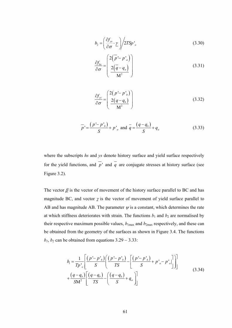
2 2 'yso

fb γ

σ∂

= ⋅ ∂ TSp (3.30)

( )( )

2

2 ' '

2

M

a

hs

a

p pf

q qσ

− ∂

= −∂

(3.31)

( )( )

2

2 ' '2

M

bys

b

p pfq qσ

−∂ = −∂

(3.32)

( )' '' 'b

a

p pp p

S−

= + and ( )ba

q qq

S−

q= + (3.33)

where the subscripts hs and ys denote history surface and yield surface respectively

for the yield functions, and 'p and q are conjugate stresses at history surface (see

Figure 3.2).

The vector β is the vector of movement of the history surface parallel to BC and has

magnitude BC, and vector γ is the vector of movement of yield surface parallel to

AB and has magnitude AB. The parameter ψ is a constant, which determines the rate

at which stiffness deteriorates with strain. The functions b1 and b2 are normalised by

their respective maximum possible values, b1max and b2max respectively, and these can

be obtained from the geometry of the surfaces as shown in Figure 3.4. The functions

b1, b2 can be obtained from equations 3.29 − 3.33:

( ) ( ) ( )

( ) ( ) ( )

1

2

' ' ' ' ' '1 ' ''

M

b b ba o

o

b b ba

p p p p p pb p

Tp S TS S

q q q q q qq

S TS S

p

− − −= − + −

− − −+ − +

(3.34)

61

( ) ( ) ( )

( ) ( ) ( )

2

2

' '1 ' ' ' ''

bb a

o

b ba

p pb p p p p

TSp S

q q q qq q

S

−= − − −

− −

+ − − Μ

(3.35)

and their maximum values are:

( )1max 2 ' 1ob p T= − (3.36)

( )2max 2 ' 1ob Tp S= − (3.37)

q

p'

b2maxb1max

Figure 3.4. Position of the surfaces when b1 and b2 are maximum.

When the history and yield surfaces are in contact, i.e.b2 = 0, the model reduces to

the two-surface model developed by Al-Tabbaa (1987). The S2 term in equation 3.26

is needed to ensure that Al-Tabbaa’s model is reproduced when the history and yield

surfaces are in contact and p'-p'b is replaced by S(p'-p'a) in equation 3.28. The

parameter T is introduced into equation 3.27 to reduce the value of H2 in order to

predict realistic strains when the stress state is inside the history surface.

62

3.2.3 Determination of Model Parameters

For the Modified Cam clay model, five parameters are required to define the model:

ecs − The voids ratio on the critical state line when p' = 1kPa.

Μ − The slope of the critical state line in the q − p' space.

-λ* − The slope of the normal compression line in ln v − ln p' space.

-κ* − The initial slope of the swelling line defined in ln v − ln p' space.

Ge − The elastic shear modulus.

For the 3-SKH model, three additional parameters are required:

T − The ratio of the size of the history surface to that of the bounding surface.

S − The ratio of the size of the yield surface to that of the history surface.

ψ − The exponent in the hardening function.

Instead of ecs, any point on the isotropic normal compression line or the critical state

line can be used to locate the model in ln v − ln p' space.

Stallebrass (1997) described a method to determine all the model parameters using

simple triaxial tests. All the model parameters, except parameter ψ, can be

determined directly. The extra parameters T and S can be determined by isotropic

swelling and recompression tests. Atkinson et al. (1990) defined recent stress history

by a sudden change in the direction of the stress path or an extended period of rest,

and used an angle ϕ to characterize the recent stress history of soil. The angle ϕ is

the angle of rotation required to follow the new stress path, and is measured positive

clockwise (see Figure 3.5), so in Figure 3.5, the angle ϕ would be negative. Figure

3.6 shows isotropic stress paths for two different stress histories, ϕ = 0o (O-B-A) and

ϕ = 180o (O-B-A-B-A). The parameters T and S can be obtained by plotting a graph

of K' against ∆p' graph as shown in Figure 3.7. The bulk modulus, K' is the tangent

stiffness obtained from the graph of p' against εp. The initial stiffness of soil

subjected to isotropic swelling (ϕ = 180o) is used to estimate κ* by plotting K'/p'

63

against p'/p'm, where p'm is the maximum mean effective pressure to which the soil

has been loaded and κ* = p'/K'. The parameter S is obtained by observing the stress

change for which the strains become inelastic, and T is obtained by estimating the

change in stress at which the two curves in Figure 3.7 converge.

The parameter ψ is the only parameter, which cannot be measured directly, and is

obtained by parametric studies. A value of ψ is chosen such that the experimental

results are best fitted.

B

Stress paths followed: O–B–A and O–B–A–B–A Stress-strain response measured twice along B–A

p'

q

Figure 3.5. Definition of recent stress history (after Atkinson et al., 1990).

A

q

Figure 3.6. Stress paths required to determine parame

Taylor, 1997).

64

O

ϕ

p'

ters T and S (Stallebrass and

∆p'

Figure 3.7. Stiffness plots from which T and S can be determined (Stallebrass and

Taylor, 1997).

3.3 ONE-DIMENSIONAL LOADING, UNLOADING AND

RELOADING

Since the 3-SKH model adopts the Modified Cam clay stress-dilatancy rule, the 3-

SKH model will over-estimate the value of K0 during normal compression and hence

shear strain (this is shown in the next section). In this section the ability of the 3-

SKH model to predict the earth pressure coefficient was investigated. The results

were obtained using the CRISP finite element program with four cubic strain

triangular elements and the parameters used in the simulation are those for kaolin

from Stallebrass (1997) given in Table 3.1.

M λ* κ* ecs T S ψ G [kN/m2]

0.89 0.073 0.005 1.994 0.25 0.08 2.5 1964(p'/p'r)0.65(p'c/p')0.2

Table 3.1. Model parameters for kaolin (Stallebrass and Taylor, 1997).

Figures 3.8 and 3.9 shows the prediction of the ‘Bubble’ model and the 3-SKH

model for K0,nc and K0 during unloading versus OCR compared to the empirical

relationship proposed by Schmidt (1966). The 3-SKH model and the ‘Bubble’ model

B-A for O-B-A-B-A

∆p' = 2TSp'o – end of elastic strains

∆p' = 2Tp'o

B-A for O-B-A

K'

65

predict a K0,nc value of 0.78 while the experimental value obtained by Al-Tabbaa is

0.69. These models will predict the same value of K0 during normal compression

because all the surfaces are in contact for normally consolidated states and therefore

both models reduce to the Modified Cam clay model. The experimental value

obtained by Al-Tabbaa is higher than that predicted by the empirical relationship

proposed by Jâky (1944) in equation 2.37 with φ' = 23° for kaolin, which gives K0,nc

= 0.61. For K0 during unloading, Al-Tabbaa found that Schmidt’s (1966) equation

2.42, with α = 0.464, fitted her data well. It can be seen from Figure 3.8 that the two-

surface model predicts a correct trend for K0 during unloading, K0,u but the value is

over-predicted significantly. The 3-SKH model gives a better prediction on

unloading, but the value of K0,u is still over predicted (see Figure 3.9). If one-

dimensional unloading is started from the correct in-situ stress state i.e. a correct

K0,nc, the 3-SKH model will give better results. The prediction of K0 during

unloading with a correct K0,nc is shown in Figure 3.10. This shows that a better

prediction of K0 during unloading can be obtained if the analysis starts from the

correct K0,nc.

0

1

2

3

4

0 2 4 6 8 10OCR

K0

12

Two-surface model

Schmidt's (1966) equation 2.42K 0,nc = 0.69

Figure 3.8. Comparison between the two-surface model prediction of K0 and the


66

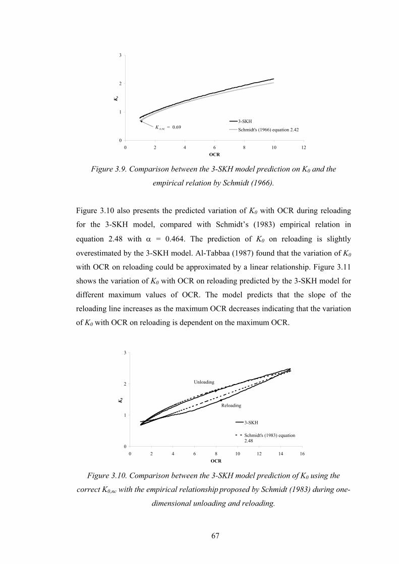
0

1

2

3

0 2 4 6 8 10 1OCR

Ko

2

3-SKH

Schmidt's (1966) equation 2.42K o,nc = 0.69

Figure 3.9. Comparison between the 3-SKH model prediction on K0 and the


Figure 3.10 also presents the predicted variation of K0 with OCR during reloading

for the 3-SKH model, compared with Schmidt’s (1983) empirical relation in

equation 2.48 with α = 0.464. The prediction of K0 on reloading is slightly

overestimated by the 3-SKH model. Al-Tabbaa (1987) found that the variation of K0

with OCR on reloading could be approximated by a linear relationship. Figure 3.11

shows the variation of K0 with OCR on reloading predicted by the 3-SKH model for

different maximum values of OCR. The model predicts that the slope of the

reloading line increases as the maximum OCR decreases indicating that the variation

of K0 with OCR on reloading is dependent on the maximum OCR.

0

1

2

3

0 2 4 6 8 10 12 14 16OCR

K0

3-SKH

Schmidt's (1983) equation2.48

Unloading

Reloading

Figure 3.10. Comparison between the 3-SKH model prediction of K0 using the

correct K0,nc with the empirical relationship proposed by Schmidt (1983) during one-

dimensional unloading and reloading.

67

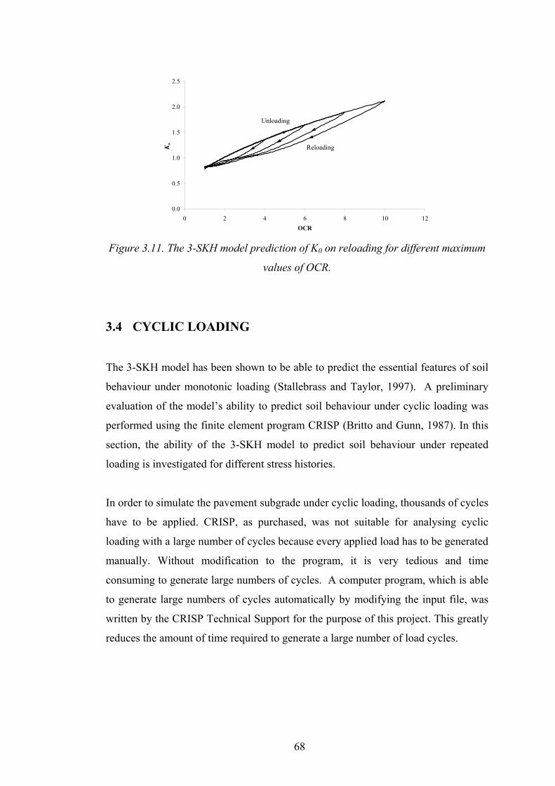
0.0

0.5

1.0

1.5

2.0

2.5

0 2 4 6 8 10OCR

Ko

12

Unloading

Reloading

Figure 3.11. The 3-SKH model prediction of K0 on reloading for different maximum

values of OCR.

3.4 CYCLIC LOADING

The 3-SKH model has been shown to be able to predict the essential features of soil

behaviour under monotonic loading (Stallebrass and Taylor, 1997). A preliminary

evaluation of the model’s ability to predict soil behaviour under cyclic loading was

performed using the finite element program CRISP (Britto and Gunn, 1987). In this

section, the ability of the 3-SKH model to predict soil behaviour under repeated

loading is investigated for different stress histories.

In order to simulate the pavement subgrade under cyclic loading, thousands of cycles

have to be applied. CRISP, as purchased, was not suitable for analysing cyclic

loading with a large number of cycles because every applied load has to be generated

manually. Without modification to the program, it is very tedious and time

consuming to generate large numbers of cycles. A computer program, which is able

to generate large numbers of cycles automatically by modifying the input file, was

written by the CRISP Technical Support for the purpose of this project. This greatly

reduces the amount of time required to generate a large number of load cycles.

68

3.4.1 Model Predictions for Repeated Loading

The model predictions for drained cyclic loading behaviour are investigated in this

section. Some existing drained cyclic loading test data on kaolin performed by Al-

Tabbaa (1987) was used to compare with the 3-SKH predictions for these tests.

Figure 3.12a shows the data for a drained cyclic test on normally consolidated

kaolin; the soil was consolidated isotropically to p' = 300kPa and then loaded

cyclically between stress ratios η of 0 and 0.34 at constant cell pressure.

(a)

εq [%]

q/p'

q/p'

εp [%]

(b)

Figure 3.12. Drained cyclic triaxial test on normally consolidated kaolin (Al-

Tabbaa, 1987) (a) q/p' versus εq and (b) q/p' versus εp.

69

Figures 3.13 and 3.14 show the predictions by Al-Tabbaa’s model and the

predictions by the 3-SKH model respectively. Both the models predict the right trend

for shear strain and volumetric strain; however, the shear strain was greatly over

predicted after four cycles. The shear strain predicted by the 3-SKH model is worse

than that of Al-Tabbaa’s model because of the smaller elastic region and different

values of ψ used by Al-Tabbaa (1987) and Stallebrass (1990). The experimental

result shows that the shear strain stabilized but both of these models cannot predict

this. The volumetric strain predicted by the models is, however, reasonable. It should

be noted that the parameters used in Figure 3.13 are those quoted by Al-Tabbaa

(1987) for kaolin, whilst those used in Figure 3.14 are those quoted by Stallebrass

(1990).

0.00

0.05

0.10

0.15

0.20

0.25

0.30

0.35

0.40

0.0 0.5 1.0 1.5 2.0 2.5 3.0

ε q [%]

q/ p

'

(a)

0.00

0.05

0.10

0.15

0.20

0.25

0.30

0.35

0.40

0.0 0.5 1.0 1.5 2.0 2.5 3.0 3.5 4.

ε p [%]

q/ p

'

0

(b)



70

0.00

0.05

0.10

0.15

0.20

0.25

0.30

0.35

0.40

0 1 2 3 4 5 6

ε q [%]

q/ p

'

(a)

0.00

0.05

0.10

0.15

0.20

0.25

0.30

0.35

0.40

0.0 0.5 1.0 1.5 2.0 2.5 3.0 3.5 4.

ε p [%]

q/ p

'

0

(b)

Figure 3.14. The 3-SKH model predictions for the test in Figure 3.12, (a) q/p' versus

εq and (b) q/p' versus εp.

Figure 3.15 shows another drained cyclic test result from Al-Tabbaa (1987) on

overconsolidated kaolin. The soil was unloaded isotropically to p' = 100kPa from p'c

= 300kPa and cyclically loaded between values of η = 0 and η = 0.78 (Al-Tabbaa,

1987). The predictions by Al-Tabbaa’s model and the 3-SKH model are shown in

Figures 3.16 and 3.17 respectively. Both Al-Tabbaa’s model and the 3-SKH model

over-predict the shear strain, but the prediction by the 3-SKH model is worse than

that predicted by the two-surface model. This is because of the inclusion of a smaller

yield surface, which causes the size of the bounding surface, p'c to decrease

significantly during isotropic unloading, and also because of the different values of ψ

used by Stallebrass (1990) and Al-Tabbaa (1987). A value of ψ of 2.5 was found

71

from parametric studies to be suitable for reconstituted kaolin by Stallebrass (1990),

whilst a ψ value of 1.5 was chosen by Al-Tabbaa (1987) to best fit data using her

two-surface model. It should be noted that this curve-fitting parameter might need to

be adjusted to better model the behaviour of soil under cyclic loading, especially if

any further amendments to the model are made.

q/p'

εq [%]

(a)

q/p'

εp [%]

(b)

Figure 3.15. Drained cyclic test result on over consolidated kaolin (Al-Tabbaa,


72

0.0

0.1

0.2

0.3

0.4

0.5

0.6

0.7

0.8

0.9

0 1 2 3 4 5 6 7 8

ε q [%]

q/ p

'

(a)

0.0

0.1

0.2

0.3

0.4

0.5

0.6

0.7

0.8

0.9

-0.5 -0.4 -0.3 -0.2 -0.1 0.0 0.1 0.2

ε p [%]

q/ p

'

(b)



Figure 3.18 shows the result of a drained cyclic load test at constant mean effective

stress on kaolin, the details of which can be found in Stallebrass (1990), together

with the prediction of the 3-SKH model. It can be seen that, again, the model over-

predicts the shear strain produced on primary loading and reloading but the model

appears to predict well the change in shear strain caused by unloading.

73

0.0

0.1

0.2

0.3

0.4

0.5

0.6

0.7

0.8

0.9

0 10 20 30 40 50 60 7

ε q [%]

q/ p

'

0

(a)

0.0

0.1

0.2

0.3

0.4

0.5

0.6

0.7

0.8

0.9

-0.3 -0.2 -0.1 0.0 0.1 0.2 0.3 0.4 0.5

ε p [%]

q/ p

'

(b)

Figure 3.17. The 3-SKH model prediction for the test in Figure 3.15, (a) q/p' versus

εq and (b) q/p' versus εp.

From the above comparisons of two-surface and 3-SKH model predictions of

drained cyclic soil behaviour, it can be seen that both models over-predict shear

strain. This problem is magnified when attempting to model cyclic loading

behaviour over many cycles, where too much shear strain will accumulate. This will,

of course, apply to the modelling of pavement subgrades: A typical three-layer

pavement problem was analysed and too much permanent deformation was predicted

using the 3-SKH model. The results of this analysis are presented in Section 3.5.

74

0

20

40

60

80

100

120

140

160

0 0.5 1 1.5 2 2

εq [%]

q [k

Pa]

.5

3-SKH

Experimental data (Stallebrass, 1990)

Figure 3.18. Constant p' test and prediction by the 3-SKH model (Stallebrass, 1990).

3.4.2 Accumulation of Negative Shear Strain

The 3-SKH model (in addition to the two-surface model) suffers a major drawback.

It was found that the model would predict an accumulation of negative shear strain,

which is not observed experimentally, under some stress conditions. To investigate

this phenomenon, conventional drained cyclic triaxial simulations were performed

on isotropically normally consolidated soil with a pre-consolidation pressure p'c =

500kPa. A deviatoric stress q of 0−50kPa was applied for five cycles. Figure 3.19

shows the predicted result of deviatoric stress versus shear strain. It can be seen that

the shear strain decrement during the unloading part of the cycle is greater than the

increment during the loading part of the cycle, due to the sudden decrease of the

stiffness on unloading, and for subsequent cycles the shear strain becomes more

negative. The rate of increase of negative shear strain is most serious during first

unloading.

The reason for the accumulation of negative shear strain is that the shear strain

developed during unloading is larger than that developed during loading. This occurs

when the stress state hits the bottom of the yield surface shown in Figure 3.20.

75

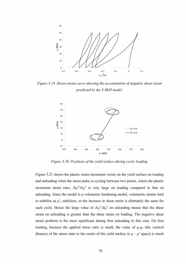
0

10

20

30

40

50

60

-0.5 -0.4 -0.3 -0.2 -0.1 0 0.1

ε q [%]

q [k

Pa]

Figure 3.19. Stress-strain curve showing the accumulation of negative shear strain

predicted by the 3-SKH model.

-10

0

10

20

30

40

50

60

470 480 490 500 510 520 530 540

p' [kPa]

q [k

Pa]

1st cycle

5th cycle

Figure 3.20. Positions of the yield surface during cyclic loading.

Figure 3.21 shows the plastic strain increment vector on the yield surface on loading

and unloading when the stress pulse is cycling between two points, where the plastic

increment strain ratio, δεpp/δεq

p is very large on loading compared to that on

unloading. Since the model is a volumetric hardening model, volumetric strains tend

to stabilise as p'o stabilises, so the increase in shear strain is ultimately the same for

each cycle. Hence the large value of δεqp/δεp

p on unloading means that the shear

strain on unloading is greater than the shear strain on loading. The negative shear

strain problem is the most significant during first unloading in this case. On first

loading, because the applied stress ratio is small, the value of q-qb (the vertical

distance of the stress state to the centre of the yield surface in q – p' space) is much

76

smaller than that on the subsequent unloading. Figure 3.20 shows the positions of the

yield surface at the end of first loading and unloading. From this figure it can be seen

that the stress state hits the yield surface at a point which would give a large negative

value of q-qb compared to that at the end of first loading. This will tend to generate

large negative shear strain. The H1 and H2 terms would help to prevent this problem,

but for small stress levels these two terms are not large enough to compensate the

loss of stiffness when the stress state hits the yield surface on unloading. The

variation of plastic hardening modulus during loading and unloading is shown in

Figure 3.22. During loading, both H1 and H2 are zero because all the surfaces are in

contact. During unloading, ho decreases due to the smaller value of p'-p'b and large

negative value of q-qb on unloading (see equation 3.24). The hardening modulus H1

is increasing because of the increase of p'o, and during unloading the stress state

never reaches the history surface, so b1 is increasing due to the increase of p'o.

During unloading, H2 is increasing at the beginning and decreasing after a certain

value. This is because of the decrease of b2 and the increase of p'o during unloading.

The increase in p'o is insufficient to overcome the decrease in b2, hence H2 increases

and then decreases. For larger applied cyclic deviatoric stresses, the H1 and H2 terms

are large enough to prevent the negative shear strain problem because the distance of

the current stress point to its conjugate stress points at the bounding surface and

history surface, b1 and b2 respectively, are larger and the size of the bounding

surface, p'o also increases. It should be noted that the increase in p'o will also

increase the values of b1max and b2max. However, the rate of increase in b1 and b2 is

larger than the rate of increase in b1max and b2max, so there is an overall increase in the

ratios of b1 and b2 to their maximum values.

Figure 3.21. Schematic d

Yieldsurface

iagram showing the yield surface and the plastic strain

increment vectors.

77

0

100,000

200,000

300,000

400,000

500,000

600,000

0 1

Number cycles, N

Har

deni

ng m

odul

us [k

Pa3 ]

h = h o +H 1+H 2

H 2

H 1

h o

Loading Unloading

Figure 3.22. Plastic hardening modulus during loading and unloading.

The effect of the model parameters and stress level on the accumulation of negative

shear strain was investigated by conducting a series of conventional drained cyclic

triaxial simulations on normally consolidated soil. The graphs of shear strain versus

number of cycles, N, are plotted in Figure 3.23-28. These graphs show the effects of

stress level and model parameters, S, T, ψ, κ*, λ* on the accumulation of negative

shear strain.

Figures 3.23 (a) and (b) shows the effect of the applied stress level on the generation

of negative shear strain during unloading. There appears to be a stress level where

the shear strain generated during loading is equal to that generated during unloading,

and hence at this stress level, there is no accumulation of shear strain. Generally the

negative shear strain problem vanishes when larger stresses are applied.

Figures 3.24−3.28 show the effect of varying model parameters. In general, for each

simulation, the values of the parameters are those in Table 3.1, except for the

parameter being varied. In Figure 3.27, S is allowed to vary so that TS is constant

(i.e. constant size of elastic region relative to the bounding surface). It can be seen

that the generation of negative shear strain is relatively insensitive to the parameters

κ* and λ*. Changing the parameters T, S or ψ will have a more influential role on the

shear strain.

78

0

50

100

150

200

250

-0.4 -0.2 0.0 0.2 0.4 0.6 0.8 1.0 1.2 1.4

ε q [%]

q [k

Pa]

(a)

-6

-4

-2

0

2

4

6

8

10

0 10 20 30 40 50 6Number of cycles, N

εq[%

]

150kPa

100kPa

70kPa

50kPa

20kPa

0

(b)

Figure 3.23. Effect of stress level on the generation of negative shear strain, (a)

stress-strain response and (b) shear strain as a function of number of cycles.

-3.0

-2.5

-2.0

-1.5

-1.0

-0.5

0.0

0.5


ε q[%

]

κ * = 0.003

κ * = 0.005

κ * = 0.008

Figure 3.24. Shear strain versus number of cycles for different κ*.

79

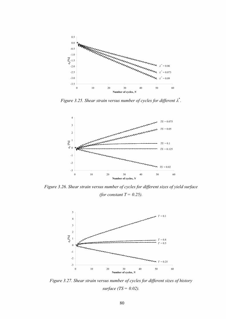
-3.5

-3.0

-2.5

-2.0

-1.5

-1.0

-0.5

0.0

0.5

0 10 20 30 40 50Number of cycles, N

ε q[%

]

60

λ * = 0.06

λ * = 0.073

λ * = 0.09

Figure 3.25. Shear strain versus number of cycles for different λ*.

-3

-2

-1

0

1

2

3

4

0 10 20 30 40 50Number of cycles, N

ε q [

%]

TS = 0.02

TS = 0.125

TS = 0.1

TS = 0.05

TS = 0.075

60

Figure 3.26. Shear strain versus number of cycles for different sizes of yield surface

(for constant T = 0.25).

-3

-2

-1

0

1

2

3

4

5


ε q[%

]

T = 0.1

T = 0.8T = 0.5

T = 0.25

0

Figure 3.27. Shear strain versus number of cycles for different sizes of history

surface (TS = 0.02).

80

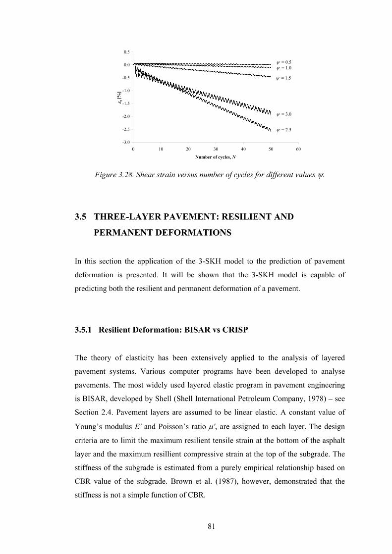
-3.0

-2.5

-2.0

-1.5

-1.0

-0.5

0.0

0.5

0 10 20 30 40 50 6

Number of cycles, N

ε q[%

]

ψ = 0.5ψ = 1.0

ψ = 1.5

ψ = 3.0

ψ = 2.5

0

Figure 3.28. Shear strain versus number of cycles for different values ψ.

3.5 THREE-LAYER PAVEMENT: RESILIENT AND

PERMANENT DEFORMATIONS

In this section the application of the 3-SKH model to the prediction of pavement

deformation is presented. It will be shown that the 3-SKH model is capable of

predicting both the resilient and permanent deformation of a pavement.

3.5.1 Resilient Deformation: BISAR vs CRISP

The theory of elasticity has been extensively applied to the analysis of layered

pavement systems. Various computer programs have been developed to analyse

pavements. The most widely used layered elastic program in pavement engineering

is BISAR, developed by Shell (Shell International Petroleum Company, 1978) – see

Section 2.4. Pavement layers are assumed to be linear elastic. A constant value of

Young’s modulus E' and Poisson’s ratio µ', are assigned to each layer. The design

criteria are to limit the maximum resilient tensile strain at the bottom of the asphalt

layer and the maximum resillient compressive strain at the top of the subgrade. The

stiffness of the subgrade is estimated from a purely empirical relationship based on

CBR value of the subgrade. Brown et al. (1987), however, demonstrated that the

stiffness is not a simple function of CBR.

81

An attempt was made to compare the results of the 3-SKH model in CRISP with

results from the layered elastic program, BISAR, which required calculating typical

vertical stress changes in the pavement using CRISP, and applying many cycles of

these stress changes to triaxial samples of 3-SKH clay in order to obtain an

equivalent stiffness for input to the elastic model.

A typical three-layer pavement was analysed using CRISP. The three-layer

pavement consisted of 50mm of bituminous material over 200 − 600mm of granular

material (sub-base) and 10m of clay (subgrade). The pavement was assumed to be

constructed in a ‘cut’ condition with typical stress history as shown in Figure 3.29.

The model subgrade was initially one-dimensionally swelled (due to erosion) from a

normally consolidated state with a value of K0,nc of 0.69, and re-compressed to model

re-deposition and construction of a pavement. This is a typical stress history for a

pavement. The swelling and recompression stress paths were applied by removing

and applying an overburden stress on the surface of the subgrade under drained

conditions. The maximum effective vertical pressure, σ'v, was assumed to be 500kPa

and the change in effective vertical stress due to erosion and re-deposition, ∆σ've and

∆σ'vr are -450kPa and 70kPa respectively. No attempt was made to simulate a

particular stress history for an existing real pavement.

p '

q

Figure 3.29. Typical stress history of a three-layer pavement.

Six-node linear strain triangular elements were used in the pavement analysis. For

the vertical boundary, radial displacements were restrained and vertical

displacements were allowed. For the horizontal boundary, both radial and vertical

82

displacements were restrained. The vertical boundaries were 5m from the axis of

symmetry and the depth of the mesh was 10m. It was shown by Almeida (1993) that

if the horizontal boundary is positioned at a distance away from the centreline of the

load of 20 times the radius of the load and the vertical boundary is positioned at a

distance away from the load of 50 times the radius of the load, then the boundary

conditions will not significantly affect the results. The effect of boundary on the

results for the pavement analyses performed in this research was found to be

insignificant.

The 3-SKH model was used to model the subgrade layer, and isotropic homogenous

linear elastic behaviour was assumed for the bituminous and granular layers. The

bituminous layer was assumed to have a Young’s modulus E' = 5,000MPa, Poisson’s

ratio µ' = 0.35 and for the granular material values of E' = 100MPa, µ' = 0.3 were

assumed. These are the typical values used in pavement analysis (Brown & Pappin,

1981). The parameters used for the 3-SKH model are shown in Table 3.1.

A typical wheel load of 42.4kN and radius of 0.15m, giving an applied surcharge of

600kPa, was applied at the top of the bituminous layer. In the pavement analysis, it

is difficult to know whether a drained or undrained analysis is appropriate. If the

subgrade is fully saturated, then the application of a single wheel load would cause

undrained deformation followed by consolidation. The passage of many wheel loads

makes this process even more complicated. It was considered to be currently too

time-consuming to perform a fully coupled consolidation analysis using CRISP with

the 3-SKH model. Furthermore, most subgrades are likely to be partially saturated,

in which case the behaviour may be more drained than undrained. In any case, it was

considered that the fully drained analysis was more relevant to the long term

behaviour of a pavement than an undrained analysis, and hence only drained

analyses of the pavement problem have been examined.

The vertical effective stress changes during the first cycle at different depths in the

subgrade were computed. The increase in effective vertical stress due to the first

application of wheel load was then applied as a deviatoric stress increment to a

triaxial sample in CRISP with a similar initial stress history for 50 cycles. Changes

83

in horizontal stress were not applied to the triaxial sample. The resilient bulk

modulus K', and shear modulus G', for the 50th cycle were then computed for

unloading. The parameters, E' and µ', needed in BISAR were then calculated. To

accommodate the variation of stiffness with depth, the subgrade was sub-divided into

three layers of thickness 0.26m, 0.9m and 8.84m, and the Young’s modulus was

calculated at the centre of each layer. Figure 3.30 shows the three-layer pavement

and the locations where the Young’s modulus were computed. The Young’s moduli

obtained for each sub-layer of subgrade with different thicknesses of granular

material are shown in Table 3.2. It can be seen that the estimated Young’s modulus

for the clay increases with increasing granular layer thickness. This illustrates that

the model is able to estimate the stiffness of the subgrade, which is stress-dependent.

The stiffness at the top layer varies quite markedly with thickness of granular

material compared to the lower layers as the vertical stresses in these two lower

layers are very small and the soil at these depths is almost elastic except for the case

where the granular material is 200mm thick, where the stiffness of the middle layer

is about 20% lower.

Stallebrass (1990) found from her experimental data that the Poisson’s ratio obtained

using equation 2.4 and 2.5 is either extremely small or negative. However, this may

be improved by adjusting the model parameter κ* in the 3-SKH model. The

parameter κ* was determined from the initial stiffness of soil subjected to isotropic

swelling with the stress path rotation of 180°. The initial stiffness is not very reliable

because measuring stiffness at very small strains is difficult. Therefore the parameter

κ* can be adjusted, since it cannot easily be determined accurately by experiment.

However, by adjusting the parameter κ*, the Poisson’s ratio obtained was still either

extremely small or negative. A ‘resilient Poisson’s ratio’ could be derived from

resilient values of shear and bulk modulus after 50 cycles. However, the value of

Poisson’s ratio found in this way was found to be unrealistic. This is because it

cannot be expected that the resilient values of G', K', E' and µ' will be consistent with

isotropic elasticity, when the material is not elastic. Therefore, for the elastic analysis

performed in this study, the Poisson’s ratio of the subgrade was taken to be 0.3. This

is consistent with the value found by Al-Tabbaa (1987) to best fit her two-surface

model with a much larger elastic region. The stress distribution at the top of the

84

subgrade clay (i.e. at the top integration points) in a three-layer pavement due to an

applied wheel load was computed, and is shown in Figure 3.31. This stress

distribution was then applied to the surface of the clay subgrade for 51 cycles as

shown in Figure 3.32. The stress change due to the applied wheel load is compared

with the stress change due to the equivalent stress blocks in Figure 3.31.

Gra

•

Figure 3.30. Schematic di

Granular layer

thickness, lg (mm) 20

E1' (MPa) 3

E2' (MPa) 8

E3' (MPa) 10

Table 3.2. Stiffness of su

600 kPa

• E'1 (Clay) 0.26m

0.9m

0.05m (asphalt)

Granular layer thickness, lg

8.84m

nular material

• E'2 (Clay)

E'3 (Clay)

agram showing the locations where the Young’s moduli, E'

are determined in the subgrade.

0 250 350 400 500 600

9 45 55 59 64 68

2 97 98 100 100 100

1 101 101 101 101 101

bgrade at centre of each layer for different granular layer

thicknesses.

85

0

5

10

15

20

25

0 1 2 3 4 5 6Distance from centreline [m]

Cha

nge

in e

ffec

tive

vert

ical

stre

ss [k

Pa]

Stress change due to applied wheelloadStress change due to equivalent stressblocks

Figure 3.31. Stress distribution near the surface of the subgrade when a typical

wheel load is applied at the surface of the bituminous layer.

Figure 3.32. Equivalent stress blocks applied at the surface of the subgrade.

The quasi-elastic settlement caused by imposing the load on the 51st cycle was

compared with the surface settlement calculated by BISAR using the elastic

parameters determined from CRISP using the 3-SKH model. Figure 3.33 shows the

typical surface profile for the 200mm granular material pavement with 50mm of

asphalt material on top predicted by the 3-SKH model at 50th unloading followed by

loading and unloading. It can be seen from this figure that the model is able to

predict both the resilient (quasi-elastic) response over one application of wheel load,

and accumulation of permanent deformation over many cycles. Figure 3.34 presents

the quasi-elastic settlement predicted by the 3-SKH model at the 51st loading and the

settlement predicted by BISAR (elastic analysis). The results show that the 3-SKH

model predictions deformation on loading are slightly larger than the results of the

BISAR elastic analysis; however they are in good agreement. The plastic strain

predicted by the 3-SKH model is responsible for the larger quasi-elastic settlement

86

for the 51st loading predicted by CRISP compared to that predicted by the elastic

analysis. Because of this, it can be seen from Figure 3.34 that the difference between

the 3-SKH prediction and the prediction from the elastic analysis is becoming

smaller as the thickness increased. The resilient deformation (i.e. recovered on

unloading, 51st unloading) predicted by the 3-SKH is also shown in Figures 3.33 and

3.34. As can be seen from Figure 3.34, the predicted resilient deformation is closer to

that predicted by the elastic analysis. This is because the stiffness calculated for

BISAR was the resilient modulus (i.e. on unloading). From the results shown, it can

be concluded that the 3-SKH model may be used to estimate the stiffness of the

subgrade for input to a layered elastic program such as BISAR instead of estimating

the stiffness from CBR values based on the empirical relationships.

-20

-18

-16

-14

-12

-10

-8

-6

-4

-2

0


Surf

ace

settl

emen

t [m

m]

50th unloading

51st loading

51st unloading

Figure 3.33. Surface profile predicted by the 3-SKH model showing the permanent

and resilient response of a pavement with 200mm granular material.

0

0.2

0.4

0.6

0.8

1

1.2

0 100 200 300 400 500 600 700Granular layer thickness [mm]

Ver

tical

def

orm

atio

n [m

m]

Elastic analysis

3-SKH (51st loading)

3-SKH (51st unloading)

Figure 3.34. Comparison between the 3-SKH model prediction and BISAR for quasi-

elastic settlement.

87

3.5.2 Permanent Deformation

One of the failure mechanisms in pavements is rutting, caused by the permanent

deformation of the pavement layers. For lightly-trafficked pavements, the

bituminous layer is relatively thin. Hence, the permanent deformation in the

subgrade is assumed to contribute most to the formation of rut, as the vertical

stresses in the subgrade layer are higher. The granular material and asphalt are

assumed to settle with the subgrade in the long term. Some additional permanent

deformation may also occur in the granular material, but the approximation has been

made here that this does not occur. Brown (1996) reported that for thinly surfaced

pavements, permanent deformations are likely to occur in the granular layer and

subgrade. He also reported the pavement experiments by Little (1993), where up to a

third of the surface rut was contributed by the granular layer, but there were cases

where the subgrade was entirely responsible for the deformation.

The major advantage of the kinematic hardening models is the ability to predict the

accumulation of strains under cyclic loading. In this section, the model predictions of

a typical three-layer pavement problem are presented. The three-layer pavement

consists of 100mm of bituminous material over a layer of granular material (sub-

base) and clay (subgrade). The bituminous and granular layers were modelled as

isotropic linear elastic, and the subgrade was modelled using the 3-SKH model. The

parameters used for the 3-SKH model are given in Table 3.1. A typical constant

wheel pressure of 600kPa was applied at the top of the bituminous layer and the

problem is axi-symmetric. This analysis presents a fundamental modeling problem:

if the material above the subgrade is assumed to be elastic, and the nodes are

common at each material interface, the elastic layers will pull the subgrade into

tension each time the pavement is unloaded. This can be overcome by calculating the

stress distribution applied at the top of the subgrade during the first application of

load, and then applying cycles of this stress distribution at the top of the clay alone

for many cycles and calculating the permanent deformation. It must then be assumed

that the granular and asphalt layers will follow the surface of the clay in the long

term. Since it is the long-term behaviour that is of interest, the clay has been

assumed to be fully drained.

88

The calculated stresses were used to apply equivalent stress blocks at the surface of

the subgrade as shown in Figure 3.32, to approximate the stress distribution at the

surface of the subgrade due to the application of wheel load. Figure 3.31 shows the

stress distribution due to the first application of load at the integration points nearest

to the top of the subgrade. This will mean that the stresses at the integration points

due to the applied stress blocks at the top of the clay alone will be slightly less than

those due to the first application of load as shown in Figure 3.31. In reality, the

bituminous and granular layers will not pull the soil into tension, and hence the

permanent settlement predicted by applying several rectangular stress blocks to the

surface of clay ought to give a more realistic result.

Figures 3.35, 3.36 and 3.37 show the predicted permanent settlement, rate of

settlement, and surface profile of the pavement subgrade respectively for different

thicknesses of granular layer as a function of number of cycles. As expected, a

thicker layer of granular material gives less settlement and a smaller rate of

settlement. The rut depth predicted by the model is considered to be too large (60mm

after 1,000 cycles for a 150mm granular layer). This is because the model over-

predicts shear strain significantly, as has already been shown in Section 3.4.1.

0

10

20

30

40

50

60

70


Perm

anen

t set

tlem

ent [

mm

] 150mm

200mm

300mm350mm400mm

500mm


distribution applied at the surface of the subgrade, showing the effect of granular

layer thickness on the predicted permanent settlement as a function of number of

cycles.

89

0.00

0.05

0.10

0.15

0.20

0.25

0 100 200 300 400 500 600 700 800 900 1000Number of cycles, N

Rat

e of

sett

lem

ent [

mm

/cyc

le]

150mm200mm

400mm350mm 500mm300mm



layer thickness on the rate of settlement with number of cycles.

-70

-60

-50

-40

-30

-20

-10

0

0 1 2 3 4 5 6

Distance from centreline [m]

Surf

ace

sett

lem

ent [

mm

]

N = 0

N = 200

N = 500

N = 1,000



layer thickness on the predicted surface profile for 150mm of granular material.

The two-surface model developed by Al-Tabbaa has also been used to model the

same pavement problem. This model does not predict any accumulation of

permanent settlement after the first loading due to the fact that the elastic region is

too large and the stress in the subgrade is well inside the yield surface.

90

3.6 SUMMARY

The formulation of the 3-SKH model has been briefly described. The ability of the

two-surface model and the 3-SKH model to predict the behaviour of soil under one-

dimensional loading, unloading and reloading, and the behaviour of soil under

drained cyclic loading has been described. It was found that these models could

reproduce some of the essential features of soil behaviour under cyclic loading.

However, by comparison with existing test data, these two models over-predict shear

strain as well as the value of K0 for normally consolidated soil. The 3-SKH model

also suffers from a problem of generating negative shear strain under some stress

conditions, which is due to the small stiffness during unloading which causes the

shear strain decrement during unloading to be greater than the increment during

loading. This negative shear strain problem only occurs under cycles of low stress

where the stiffness during unloading is too small. Because the model over-predicts

shear strain, this problem is magnified when the model is applied to cyclic loading

behaviour where large numbers of cycles are involved. This will predict unrealistic

deformation when analysing a pavement problem where large numbers of cycles are

applied.

Pavement foundations are best described within the framework of critical state soil

mechanics (Brown, 1996). The 3-SKH model has been applied in a pavement

analysis to predict the resilient and permanent response of a pavement. The resilient

response on unloading predicted by the 3-SKH model agrees well with the results

from a multi-layered elastic analysis. However, the rut depth predicted by the 3-SKH

model is too large. The two-surface model is not suitable for the prediction of the

permanent response of a pavement as the elastic region for this model is too large

and no accumulation of permanent strain is predicted by this model. Consequently,

an alternative model is required which will reduce the amount of predicted shear

strain. This is the subject of the next chapter.

91

4 FORMULATION OF A SIMPLE NON-ASSOCIATED

THREE-SURFACE KINEMATIC HARDENING

MODEL

4.1 INTRODUCTION

It has been shown in the previous chapter, that the 3-SKH model over-predicted the

value of Ko for normally consolidated soil, and the model also over-estimated shear

strain. This problem becomes significant when the model is used to model behaviour

of clay subjected to cyclic loading, where too much shear strain accumulates over

many cycles. Modification of the flow rule may give a better prediction of K0 for

normally consolidated soil and the shear strain induced by cyclic loading, and this

will also affect the problem of generation of negative shear strain. The negative shear

strain problem may be eliminated by modifying the hardening modulus.

This chapter describes the mathematical formulation of the new non-associated

three-surface kinematic hardening model. The new model has been derived by

modifying the flow rule of the 3-SKH model to allow more flexibility of the shape of

the plastic potential. The critical state dissipation constant M was also made to be a

function of Lode angle in stress space. The translation rules of the 3-SKH model

have been retained. An extra parameter is required in the model to control the shape

of the plastic potential, and by choosing an appropriate value for the new parameter,

the amount of the shear strain predicted can be controlled. However, the problem of

generation of negative shear strain still remains under certain stress conditions, and

this causes the rut depth to decrease after a number of cycles when analysing the

repeated loading of a pavement. The hardening modulus of the model was therefore

modified in order to solve this problem and a new parameter was introduced; various

expressions of the hardening modulus have been adopted and are presented in this

chapter.

92

4.2 NON-SYMMETRICAL FLOW RULE To improve the amount of shear strain predicted by the 3-SKH model, an attempt

was made to change the flow rule. The flow rule proposed by McDowell (2000),

described in Section 2.2.7 was adopted. This flow rule states that for points on the

bounding surface, the ratio of the plastic strain increments is:

1 1d

d

p a app a

q

ε ηε η

+ +Μ −= (4.1)

and the plastic potential on the bounding surface is:

( ) ( )1

1M ' 1 ln 2 ' ' apq p a p p + = + (4.2)

where a is a constant controlling the shape of the potential, and p'p is the hardening

parameter for the potential.

From the flow rule the plastic potential for the yield surface was derived by

translation of the origin in equation 4.2, giving the equation of the plastic potential in

triaxial stress space:

( )1

12 '( ' ' ' ) ( 1) ln 0

' ' '

ap

b b ob o

TSpq q p p TSp a

p p TSp

+ − − Μ − + + = − +

(4.3)

The hardening parameter p'p can be obtained by substituting the current values of p'

and q into equation 4.3 and solving for p'p.

The hardening rule, which links δp'o with the plastic volumetric strain, is the same as

that used by Modified Cam clay:

* *

'' poo

pp pδ δελ κ

=−

(4.4)

93

Since we know that the plastic strain increment vector is always normal to the plastic

potential:

qgpg

pq

pp

∂∂

=

∂∂

=

χδε

χδε' (4.5)

where χ is a scalar multiplier.

The plastic strain increment on the yield surface can be found by combining the

translation rule, consistency equation, hardening rule, and equation 4.5. The general

expression for the plastic strain increment in triaxial stress space is:

∂∂

⋅∂∂

∂∂

⋅∂∂

∂∂

⋅∂∂

∂∂

⋅∂∂

×

∂∂

⋅∂∂

⋅

∂∂

+∂∂

+∂∂

−=

qp

qg

qf

qg

pf

pg

qf

pg

pf

pgp

pq

qf

pp

pf

pf

pp

o

o

b

bo

b

bo

pq

pp

δδ

εδεδε '

'

'''

''

'''

''

1 (4.6)

Substituting the derivatives of the yield surface and plastic potential for the model

into equation 4.6 gives:

( ) ( ) ( ) ( )

( )( ) ( )

−−−

+−

−

−+−

−−

×=

+−

++−

+

qp

qqqqpp

TSpppBBqq

TSpppBBpp

h

bbb

obaab

obaa

b

op

q

pp

δδ

δεδε

'

MM''

'''M

'''''

1

2

22

121

12

21

211

2

(4.7)

where:

( ) ( ) ( )2 21

1 12

* *

' ' ' ' ' 'M

b a ab b

o

q q qop p p B B p p TSp

hλ κ

−+ +

−− + ⋅ − ⋅ − +

=−

(4.8)

94

and:

( )2 '

1 ln' ' '

p

b o

TSpB a

p p TSp

= + − + (4.9)

However, it was found to be very difficult to implement this flow rule into the 3-

SKH model: the hardening modulus terms H1 and H2 in equations 3.26 and 3.27, need to be modified because the hardening modulus ho is different from that in the 3-

SKH model. In addition, there are six singularity points at which unlimited strains

will be predicted. Two of these are the same as the two-surface model and the 3-

SKH model; that is when the dot product of the vector joining the origin to the

current stress state and the vector normal to the yield surface at that stress point is

equal to zero − see Section 3.2.2. Two other singularity points are when B = 1, this

happens when p'-p'b = 0: i.e. at the top and bottom apexes. At these singularity

points, infinite plastic strain is predicted. Another singularity point is when p'-p'b = -

TSp'o at which ho = 0. This occurs when the stress point is at the left apex of the yield

surface. However, the terms H1 and H2 may resolve this problem. The sixth

singularity point occurs during isotropic normal compression. At this point, B = 0

and the plastic strain increment is undefined. Due to the complexity of this flow rule,

it was abandoned and another simpler flow rule, which is symmetrical about the

centreline of the yield surface and which will not introduce any extra singularity

points, was proposed.

4.3 THE NON-ASSOCIATED THREE-SURFACE KINEMATIC

HARDENING MODEL

In this section the derivation of the new non-associated model is described. The

methods used to derive this model are largely similar to those used by Al-Tabbaa

(1987) and Stallebrass (1990) to derive the two and three-surface models

respectively, which are extensions of the Modified Cam clay model.

95

4.3.1 Model Description

This model has been derived within the framework of Critical State Soil Mechanics

and it is an extension to the 3-SKH model developed by Stallebrass (1990). It has a

Modified Cam clay yield surface in triaxial stress space as shown in Figure 3.1.

The outermost surface is now not a true yield surface, which encloses the truly

elastic region, following the terminology used by Al-Tabbaa (1987) and Stallebrass

(1990), this surface is called the ‘bounding surface’, with the inner two kinematic

surfaces being the ‘history surface’ and ‘yield surface’ as described in Chapter 3.

These two kinematic surfaces have the same shape as the bounding surface but are

smaller in size, with this size expanding and contracting at a fixed ratio. The

equations for the bounding, history and yield surface in the triaxial stress space are

still as given in equations 3.1 - 3.3.

4.3.2 Stress-dilatancy Rule

The 3-SKH model is assumed to obey the normality rule i.e. the plastic potential is

identical to the yield surface. Since the bounding surface is of the Modified Cam

clay type, this will lead to an over prediction of shear strain and K0,nc. The plastic

strain increment ratio on the bounding surface is:

2 2d M

d 2

ppp

q

ε ηε η

−= (4.10)

In order to reduce the amount of shear strain predicted by the 3-SKH model, a new,

simple and more flexible expression for the flow rule was proposed:

2 2d M

d

ppp

q kε ηε η

−= (4.11)

96

which requires the specification of one additional new parameter k. This flow rule

was also proposed by Ohmaki (1982) to predict correctly the value of K0,nc and used

by Alonso et al. (1990) to model the behaviour of partially saturated clays.

This flow rule is associated at critical states and also for isotropic conditions, but

non-associated between these points, where the plastic strain increment ratio at a

given stress ratio depends on the value of k. This was implemented into the 3-SKH

model to improve its prediction of K0,nc and hence shear strain. To illustrate the effect

of using different values of k on the plastic strain increment vector, Figure 4.1 shows

the directions of the plastic strain increment vectors for k = 0.5 and 1.0. The slope of

the plastic strain increment vector has been reduced compared to that when the

normality condition is applied (i.e. k = 2). This will reduce the plastic shear strain

predicted by the model by a factor of 2/k. By choosing an appropriate value of k, the

value of the coefficient of earth pressure at rest during one-dimensional compression

Ko,nc can be predicted more accurately than the 3-SKH model. The predicted results

for the value of the coefficient of earth pressure at rest during one-dimensional

loading, unloading and reloading are presented in section 4.3.7.

The plastic potential, g, can be obtained by integration of equation 4.11:

( )2

2 222 M ' M '2 ' 01 2 ' 1-

k

pp

pg q pk p k

= + − = −

2p (4.12)

except for k = 1 when

( ) 0'/'2ln2'M =−= pppqg p (4.13)

where p'p is the hardening parameter for the plastic potential.

97

0

0.1

0.2

0.3

0.4

0.5

0.6

0.7

0 0.2 0.4 0.6 0.8 1 1.2

p' /(2p' o )

q/(2

p'o)

Non-associated flow, k = 1Associated flow

(a)

0

0.1

0.2

0.3

0.4

0.5

0.6

0.7

0 0.2 0.4 0.6 0.8 1 1.2

p'/(2p' o )

q/(2

p'o)

Non-associated flow, k = 0.5Associated flow

(b)

Figure 4.1. Comparison between associated and non-associated flow plastic strain

increment vectors (a) k = 1, and (b) k = 0.5.

The shape of the plastic potential can be varied by using different values of k. The

effect of parameter k on the shape of the plastic potential is shown in Figure 4.2.

By translation of the origin in equation 4.9, the plastic potential for the yield surface

is therefore:

98

( ) ( ) ( )2

222

2

' ' '' ' '1 2 '1 2 ' 1

kb ob b o

pp

p p TSpq q p p TSpg TSpk TSp k

− +− − += + − Μ − −

0= (4.14)

except for k = 1, when

( ) ( )2 '

M ' ' ' 2 ln 0' ' '

pb b o

b o

TSpq q p p TSp

p p TSp

− − − + = − + (4.15)

0

0.1

0.2

0.3

0.4

0.5

0.6

0.7

0.8

0 0.2 0.4 0.6 0.8 1 1.2p'/(2p' p )

q/(2

p'p)

k = 0.5

k = 1

k = 2

Figure 4.2. Plastic potentials for various values of k.

4.3.3 Hardening Rule

The way the hardening modulus is derived is the same as that used for the 3-SKH

model; it is derived from the special case when all the surfaces are in contact, and is

then generalised. However, there is a slight modification to the hardening moduli H1

and H2 of the new model. The hardening rule, which links δp'o with the plastic

volumetric strain, is the same as that used by Modified Cam clay − see equation 4.4.

Substituting the derivatives of the yield surface and plastic potential for the model

into equation 4.6 results in the following expression for the plastic strain increment

on the yield surface:

( ) ( ) ( )

( ) ( ) ( )

−−−

−−−

×=

qp

qqqqpp

qqpp

kpp

kh bb

b

bbb

op

q

pp

δδ

δεδε '

MM''

M''2''2

1

4

2

2

22

(4.16)

where the hardening modulus ho is:

99

( ) ( ) ( )2

* *

2' ' ' ' 'bb b

o

q q qp p p p p

M kλ κ

−− + ⋅ −

=−

h (4.17)

Note that the hardening modulus ho is reduced to that of the 3-SKH model when k =

2, and that only shear strains are affected for given values of p', q, δp', δq', p'b and qb

(i.e. for a given stress path).

This hardening modulus, ho, will predict infinite plastic strains at four singularity

points, which are the same as those in the 3-SKH model. Hence the hardening

moduli, H1 and H2, can be used without major modification. Detailed description of

the singularity points can be found in Al-Tabbaa (1987) and has been briefly

described in Chapter 3. Because of this instability region, described in Section 3.2.2,

Stallebrass (1990) defined the hardening modulus h as a function h = ho + H1 +H2.

Hashiguchi (1985) expressed the hardening modulus as a function of the degree of

approach of the surfaces such that the hardening modulus is zero when the surfaces

are in touch. Following this, Stallebrass (1990) expressed H1 as a function of b1, the

degree of approach of the history surface to the bounding surface and H2 as a

function of b2, the degree of approach of the yield surface to the history surface. The

H1 and H2 terms for the new model are slightly different from those used by the 3-

SKH model; a factor of 2/k has been applied to these terms:

3 211 * *

1max

1 2 'obH

k b

ψ

λ κ

= − p S (4.18)

322 * *

2max

1 2 'oT bH

k b

ψ

λ κ ⋅

= − p (4.19)

the terms in these equations were explained in Section 3.2.2.

By using these expressions for H1 and H2, ho, H1 and H2 are all scaled by 2/k so that

the value of parameter k will affect only the plastic shear strain and not the plastic

volumetric strain for given values of p', q, δp', δq', p'b and qb, so that the plastic

100

volumetric strain predicted by the new model will be the same as that predicted by

the 3-SKH model. This is considered acceptable because Al-Tabbaa (1987) showed

that volumetric strains were predicted well for kaolin by her two-surface model.

Thus, the constitutive relationship for the plastic strain increments is:

( ) ( ) ( )

( ) ( ) ( )

−−−

−−−

×=

qp

qqqqpp

qqpp

kpp

kh bb

b

bbb

pq

pp

δδ

δεδε '

MM''

M''2''2

1

4

2

2

22

(4.20)

where:

( ) ( ) ( )

* *

3 2 31 22

1max 2max

1

2 2 2' ' ' ' ' ' 'bb b o

h

q q q b Tbp p p p p p S pk k b k b

ψ ψ

λ κ= ×

− − − + ⋅ − + + Μ

o

(4.21)

The expressions for H1 and H2 are certainly not unique and can be modified to

improve predictions. It will be shown that these expressions are not suitable for

analysing a pavement problem where the stresses in the pavement foundation are

relatively small. In Section 4.3.8, different expressions of the hardening modulus are

proposed in order to improve the model predictions under cyclic loading.

4.3.4 Yield Surface and Plastic Potential in Deviatoric Plane

For the ‘Bubble’ model and the 3-SKH model, the critical state dissipation constant

M is assumed to be constant. However, it is well known that the Mohr-Coulomb

criterion is more appropriate to failure conditions in soils (Potts and Zdravković,

1999), so that the critical state constant M is a function of Lode angle in stress space.

In the new model, the critical state dissipation constant M has been made to be a

function of Lode angle, θ according to the expression proposed by Sheng et al.

(2000):

101

( )

144

4 4

2M M1 1 sin 3c

αα α θ

= + + −

(4.22)

M 3 sin ' 3M 3 sin ' 3 M

e

c c

φαφ

−= = =

+ + (4.23)

( )( )

2 31

1 3

' '1tan 2 1' '3

σ σθ

σ σ−

−= − −

(4.24)

where Mc is the value of M in triaxial compression with θ = -30°, and Me is the value

of M in triaxial extension θ = 30°. The parameter φ' is the friction angle of the soil at

a critical state, assumed to be independent of Lode angle. Figure 4.3 shows the

failure surface in the deviatoric plane, having a similar shape to that proposed by

Matsuoka and Nakai (1974). This surface coincides with the Mohr-Coulomb

hexagon at all vertices in the deviatoric plane, and the failure surface remains convex

if α ≥ 0.6 (i.e. φ' ≤ 48.59° or Mc ≤ 2) which is common for most clays (Sheng et al.,

2000).

σ ' 1

θ = -30o

θ = 30o

σ ' 2

σ ' 3

Original 3-SKH New model (M varies according to Sheng et al.

(2000))

Mohr-Coulomb

Figure 4.3. Failure surface in deviatoric plane given by equation 4.22.

102

In the new model, the shape of the yield surface, history surface, bounding surface

and potential have all been assumed to have a shape in the deviatoric plane given by

equation 4.22, and the Lode angle is calculated for the current point in stress space

using a floating origin at the centre of the yield surface. For simplicity, the rate of

change of the value M with respect to Lode angle, ∂M/∂θ, is assumed to be

negligible. This implies that the yield surface and the plastic potential in the

deviatoric plane remain circular in shape with the radius changing according to

equation 4.22. This assumption will make the mathematical formulation much

simpler and is justified in the next section by a typical boundary value problem using

the model described by Yu and Khong (2002). The effect of ∂M/∂θ will be important

for the potential under plane strain conditions (Potts and Zdravković, 1999).

4.3.5 Justification of ∂M/∂θ = 0

In order to justify the assumption that the rate of change of M with respect to Lode

angle is negligible, finite element analyses on footing problems using the model

developed by Yu (1998) have been performed. This model was fully implemented in

CRISP by Yu and Khong (2002), which also used the relationship between M and

Lode angle (equation 4.22) proposed by Sheng et al. (2000). Three versions of this

model have been implemented in CRISP: (1) M varies according to equation 4.22

with ∂M/∂θ = 0 for both the yield surface and the plastic potential in the deviatoric

plane: i.e. circular shape, (2) M varies according to equation 4.22 for both the yield

surface and plastic potential, and ∂M/∂θ is allowed to vary according to equation

4.22 for both the yield surface and plastic potential (i.e. both the yield surface and

plastic potential are of the Sheng et al. (2000) shape in Figure 4.3), and (3) M varies

according to equation 4.22 for both the yield surface and the plastic potential, but

∂M/∂θ is zero for the plastic potential only (i.e. circular potential and Sheng et al.

(2000) type yield surface).

A rigid circular footing and a strip footing were analysed using these models to

investigate the effect of the shape of the yield surface and plastic potential in the

103

deviatoric plane. The finite element mesh used to analyse the footing problems is

shown in Figure 4.4. Cubic strain triangle elements were used in the analyses.

Figure 4.4 . Finite element mesh for footing problem.

The model parameters chosen are relevant to London clay (Yu and Khong, 2002).

The first problem was a rigid circular footing under undrained loading conditions

and the second problem was a rigid strip footing under the same loading conditions.

Figures 4.5 and 4.6 show the plot of applied pressure against displacement for the

circular footing and strip footing respectively. The first and second letters in the

figure denote the shape of the yield surface and plastic potential in the deviatoric

plane respectively, where ‘s’ denotes Sheng et al. (2000) type surface and ‘c’ a

circular shape. For a circular footing (axi-symmetry), the shapes of the yield surface

and plastic potential in the deviatoric plane were found to be insignificant. However,

the shape of the plastic potential in the deviatoric plane was found to be more

significant for the plane strain problem. However, the shape of the yield surface in

the deviatoric plane had no effect on the plane strain problem. These findings agree

with the findings of Potts and Gens (1984) who showed that, in plane strain

problems, the shape of the plastic potential in the deviatoric plane has a dominating

influence on the predicted behaviour especially for drained conditions. According to

Potts and Gens (1984), the plastic potential should predict the correct Lode angle at

failure, θf, and the predicted value of θf affects the predictive capability for plane

strain deformation. As for the effect of the yield surface, Potts and Gens (1984) also

noticed that in their plane strain problem, this has little influence on the predictions,

so long as the correct value of φ' at failure was produced. Hence, for simplicity, the

104

new model proposed in this research assumed that both the shape of the plastic

potential and yield surface in the deviatoric plane were circular (i.e. ∂M/∂θ = 0), with

the value of M varying with Lode angle according to equation 4.22. Further work is

needed to justify this assumption for the new model.

0

50

100

150

200

250

300

350

0 0.05 0.1 0.15 0.2 0.25 0.3 0.35Displacement [m]

App

lied

stre

ss [k

Pa]

s,s

s,c

c,c

Figure 4.5. Results predicted by CASM (Yu, 1998; Yu & Khong, 2002) showing the

effect of the shape of yield surface and plastic potential in the deviatoric plane for a

circular footing (axi-symmetric problem).

0

50

100

150

200

250

300

0 0.05 0.1 0.15 0.2 0.25 0.3 0.35

Displacement [m]

App

lied

pres

sure

[kPa

]

s,s

s,c

c,c

Figure 4.6. Results predicted by CASM (Yu, 1998; Yu & Khong, 2002) showing the

effect of the shape of yield surface and plastic potential in the deviatoric plane for a

strip footing (plane strain problem).

105

4.3.6 Generalisation of Model, Finite Element Implementation and

Validation of the New Model in CRISP

To perform non-linear finite element analysis using elasto-plastic models, it is

necessary to compute the elastic-plastic matrix, [Dep] relating an increment of strain

to an increment of stress:

{ } [ ]{ }εσ ∆=∆ epD (4.25)

There is a standard method to obtain the expression for the elastic-plastic matrix,

[Dep], which can be found in standard finite element textbooks such as Potts &

Zdravković (1999):

[ ] [ ][ ] [ ]

[ ] HgDf

DfgDDD

e

ee

eep

+

∂∂

∂∂

∂∂

∂∂

−= Τ

Τ

''

''

σσ

σσ (4.26)

where [De] is the elastic matrix and H is the hardening/softening modulus. For the

three-surface model:

1oH h H H2= + + (4.27)

where ho is given by:

' '

' ' 'bij o

oo bij o ii

p'ii

f fhp p

σ gσ ε σ

∂∂ ∂= − + ∂ ∂ ∂ ∂

∂ (4.28)

In order to implement the model into a finite element code, the model has to be

formulated in general stress space. The equations of the yield surface and plastic

potential are written in general stress space by substituting q with deviatoric stress

tensor, the equations of the yield surface, f and plastic potential, g become:

106

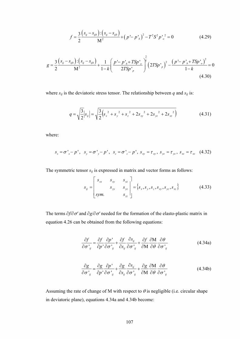
( ) ( ) ( )2 2 2 22

:3 ' ' '2

ij ijb ij ijbb o

s s s sf p p

− −0T S p= + − − =

Μ (4.29)

( ) ( ) ( ) ( )2

22

2

: ' ' '' ' '3 1 2 '2 1 2 ' 1

kij ijb ij ijb b ob o

pp

s s s s p p TSpp p TSpg TSpk TSp k

− − − +− += + − Μ − −

0=

(4.30)

where sij is the deviatoric stress tensor. The relationship between q and sij is:

( )222222 22223

23

xzyzxyzyxij sssssssq +++++== (4.31)

where:

' 'x xs pσ= − , ' 'y ys pσ= − , ' 'z zs pσ= − , xyxys τ= , yzyzs τ= , xzxzs τ= (4.32)

The symmetric tensor sij is expressed in matrix and vector forms as follows:

{ xzyzxyzyx

zz

yzyy

xzxyxx

ij ssssssssymsssss

s ,,,,,.

=

= } (4.33)

The terms ∂f/∂σ' and ∂g/∂σ' needed for the formation of the elasto-plastic matrix in

equation 4.26 can be obtained from the following equations:

'' ' ' '

ij

ij ij ij ij ij

sf f p f fp s '

θσ σ σ θ σ

∂∂ ∂ ∂ ∂ ∂ ∂Μ ∂= + +

∂ ∂ ∂ ∂ ∂ ∂Μ ∂ ∂ (4.34a)

'' ' ' '

ij

ij ij ij ij ij

sg g p g gp s '

θσ σ σ θ σ

∂∂ ∂ ∂ ∂ ∂ ∂Μ ∂= + +

∂ ∂ ∂ ∂ ∂ ∂Μ ∂ ∂ (4.34b)

Assuming the rate of change of M with respect to θ is negligible (i.e. circular shape

in deviatoric plane), equations 4.34a and 4.34b become:

107

'' ' '

ij

ij ij ij ij

sf f p fp s 'σ σ σ

∂∂ ∂ ∂ ∂= +

∂ ∂ ∂ ∂ ∂ (4.35a)

'' ' '

ij

ij ij ij ij

sg g p gp s 'σ σ σ

∂∂ ∂ ∂ ∂= +

∂ ∂ ∂ ∂ ∂ (4.35b)

All the terms required for the elasto-plastic matrix can be found in the appendix.

From the definition of the Lode angle, equation 4.24, it should be noted that there is

a discontinuity of Lode angle from σ'v> σ'h to σ'h > σ'v i.e. from compression to

extension (i.e. at an isotropic stress state), the Lode angle is undefined. However, this

should not create any difficulties in the implementation of the new model into a

finite element code, because at this point, the flow rule is not affected by the Lode

angle and hence any value of Lode angle can be assumed at this point. At isotropic

stress states, only volumetric strains occur (the plastic strain increment ratio

dεpp/dεq

p, is equal to infinity), so any value of the Lode angle can be assumed at this

point.

The original 3-SKH model was implemented in CRISP and the new model was

implemented by amending the source code for the original 3-SKH model. The new

flow rule with constant M was first implemented followed by the implementation of

M as a function of Lode angle. After the implementation, the program was tested by

the following methods to ensure that the implementation was correct:

1. Constant M

• For the new model with constant M, it was ensured that the results predicted

were the same as the original model for k = 2.

• For other values of k, it was ensured that the shear strain predicted by the new

model was approximately k/2 times the shear strain predicted by the original

108

model (the relationship is approximate because the factor 2/k applies to

plastic strains only).

• The volumetric strain predicted by the new model should be exactly the same

as that predicted by the original model for any value of k for a given stress

path.

2. Varying M

• After the new model with varying M was implemented, a triaxial extension

simulation was performed to ensure that the soil reached a critical state at a

stress ratio equal to Me. This critical state stress ratio could be calculated

from Mc using equation 4.23.

• In addition, an undrained triaxial simulation was performed with all the

surfaces initially centralised. The model should predict a straight line for the

undrained stress path in the q − p' space.

The model predicted the correct response for all these loading paths.

4.3.7 Evaluation of the New Model

It has been shown in Chapter 3 that the 3-SKH model is able to capture most of the

essential features of cyclic loading of soil behaviour. However, this model over

predicts K0,nc and shear strain on loading. Figure 3.18 shows that the 3-SKH model

greatly over-predicts shear strain for a shear test at constant p', and it has also been

shown that in Figure 3.9 the earth pressure coefficient at rest during normal

compression and unloading is over-estimated. By changing the flow rule of the 3-

SKH model, the predicted shear strain can be scaled down and hence the earth

pressure coefficient at rest can be correctly predicted – at least for normally

consolidated conditions. It was considered that if the value of k could be found such

that the model correctly predicted K0,nc, then this would result in better predictions of

shear strain for a given cyclic stress path. According to McDowell and Hau (2003)

109

the value of k required to correctly predict K0,nc may be estimated from equation

4.11, neglecting elastic strains, so that for one-dimensional conditions:

2 2

1

1

d d M1.5d 2d 3

p

q kε ε ηε ε η

−= = = (4.36)

where the critical state parameter M in triaxial compression is related to the critical

state angle of friction φ', according to the equation:

6sin 'M3 sin '

φφ

=−

(4.37)

The effect of k on values of K0 during normal compression for different values of φ'

is also shown in Figure 4.7.

0

0.1

0.2

0.3

0.4

0.5

0.6

0.7

0.8

0.9

0 0.2 0.4 0.6 0.8 1 1.2 1.4 1.6 1.8 2

k

K0,

nc

φ ' = 20ο

φ ' = 25ο

φ ' = 30ο

φ ' = 35ο

Figure 4.7. Effect of parameter k on the prediction of K0 at normally consolidated

state.

For kaolin, Al-Tabbaa (1987) obtained a value of K0,nc = 0.69 (η0,nc = 0.39) and M =

0.89. Substituting these values into equation 4.36 gives k = 1.1. For soils that satisfy

the Jâky (1944) equation 2.37, the stress ratio η0,nc during one-dimensional

compression is given approximately by the equation:

0, 0.6Mncη ≈ (4.38)

110

Equation 4.38 can be verified by substituting different values of φ' into equations

2.37 and 4.37. Substituting equation 4.38 into equation 4.11 for one-dimensional;

conditions with dεpp/ dεq

p = 1.5 (i.e. neglecting elastic strains) gives:

0.7Mk ≈ (4.39)

for such soils.

Figure 4.8 shows the prediction of K0,nc of the new model with k = 0.7M for different

angles of friction compared with the values predicted by the 3-SKH model and

various relationships proposed by other researchers (Jâky, 1944; Brooker & Ireland,

1965; Bolton, 1991b; Simpson, 1992) which have been described in Section 2.2.9.

The result shows that the new model has greatly improved the prediction of K0,nc

compared to the original model which over-estimates K0,nc.

0.3

0.4

0.5

0.6

0.7

0.8

0.9

20 22 24 26 28 30 32 34 36 38 40φ ' [o]

K0,

nc

New model; k = 0.7M

Brooker & Ireland 'BRICK' model

JâkyBolton

3-SKH

Figure 4.8. Comparison of the values of K0,nc predicted by the new model and by

other models.

Figure 4.9 shows the prediction of the K0 for kaolin during loading, unloading and

reloading by the new model with a constant value of M, and with M varying

according to equation 4.22, using a value of k = 1.1. This value of k would give K0,nc

= 0.684 (η0,nc = 0.40) which agrees well with the value of K0,nc = 0.69 obtained by

Al-Tabbaa (1987). According to equation 4.11 with η0,nc = 0.40, the value for

dεpp/dεq

p is 1.44. This illustrates that the elastic strains can be neglected in the

111

determination of the value of k. It can be seen that the prediction of the value of K0

during normal compression is better than the original 3-SKH model. Figure 4.9,

curve A, shows the values of K0 predicted by equation 2.48. The values predicted by

the new model with constant M are given by curve B. It can be seen that the

prediction of K0 on unloading is worse than that given by the 3-SKH model (curve

C). It was considered that this was because the stress ratio at failure, M, had been

assumed to be independent of the Lode angle in stress space. The effect of allowing

M to be a function of Lode angle, on the predicted value of K0 for primary

unloading, is given in Figure 4.9, curve D. It can be seen that the prediction is much

better than that given by using a constant value of M (curve B), and is better than the

3-SKH model (curve C). If required, k could be permitted to be different under

compression and extension conditions. This is equivalent to applying a different flow

rule in compression and extension. A suitable formulation in generalised stress

space, following equations 4.22 – 4.24, would be:

( ) ( )

144

c 4 4

21 1 sin 3

k k αθα α θ

= + + −

(4.40)

e

c

kk

α = (4.41)

where ke relates to triaxial extension (θ = +30°) and kc to compressive (θ = -30°)

conditions. The value of α could be determined by trial error. A constant value of k

may be insufficient to fit both the values of K0,nc and K0 on unloading. Equations

4.40 and 4.41 are useful for this purpose.

For reloading, curve A in Figure 4.9 shows the empirical relation proposed by

Schmidt (1983) given by equation 2.48 with OCRmax = 10. The prediction of the 3-

SKH model is also shown (curve C), together with the new model using k = 1.1

(curve D). It appears that the 3-SKH model is better than the new model, but this is

mainly because of the higher value of of K0,nc. The prediction of K0 on reloading

cannot be expected to be correct, as the model exhibits strong ratcheting under

112

drained cyclic loading: this is a function of the H1 and H2 terms in the hardening

modulus.

0

1

2

3

4

0 2 4 6 8 10 12 14 16

OCR

K0

Curve B: k = 1.1, constant M

Curve D: k = 1.1, M given by equation 4.22

Curve C: 3-SKH

Curve A: Schmidt (1983), equation 2.48

Figure 4.9. Comparison between model predictions of K0 and empirical result.

It was considered that if the value of k could be found such that the model correctly

predicted K0,nc, then this would result in a better prediction of shear strain. Figure

4.10 shows the predictions of the original model and the new model (with M given

by equation 4.22) for the constant p' drained cyclic loading test performed by

(Stallebrass, 1990) – see Figure 3.18. It can be seen that the shear strain predicted

has been greatly improved by the new model. However, the shear strain on reloading

is still over-predicted. As pointed out by Stallebrass (1990), this is because the

stiffness drops rapidly when the stress state reaches the history surface, and a more

appropriate expression for H1 may improve this. In addition, the ratcheting

phenomenon is still exhibited by the new model as seen in Figure 4.10, but the

increase in shear strain caused by the unload – reload cycle is reduced by about 40%.

113

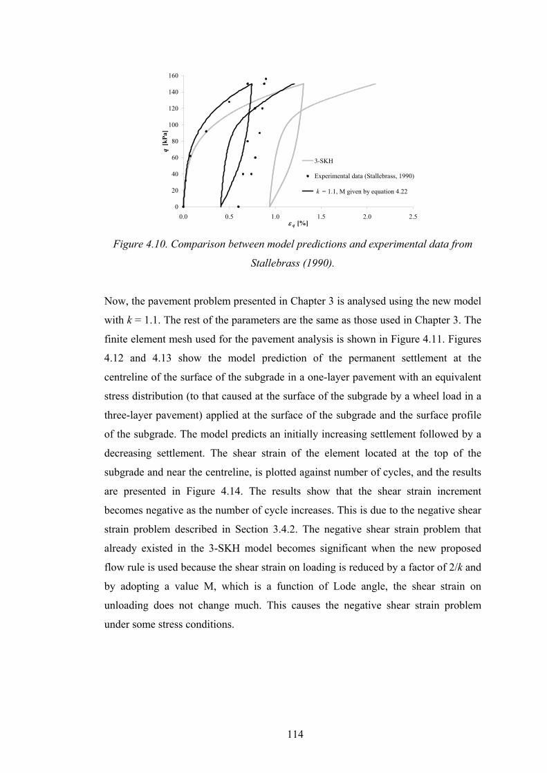
0

20

40

60

80

100

120

140

160

0.0 0.5 1.0 1.5 2.0 2.5ε q [%]

q [k

Pa]

3-SKH

Experimental data (Stallebrass, 1990)

k = 1.1, M given by equation 4.22

Figure 4.10. Comparison between model predictions and experimental data from

Stallebrass (1990).

Now, the pavement problem presented in Chapter 3 is analysed using the new model

with k = 1.1. The rest of the parameters are the same as those used in Chapter 3. The

finite element mesh used for the pavement analysis is shown in Figure 4.11. Figures

4.12 and 4.13 show the model prediction of the permanent settlement at the

centreline of the surface of the subgrade in a one-layer pavement with an equivalent

stress distribution (to that caused at the surface of the subgrade by a wheel load in a

three-layer pavement) applied at the surface of the subgrade and the surface profile

of the subgrade. The model predicts an initially increasing settlement followed by a

decreasing settlement. The shear strain of the element located at the top of the

subgrade and near the centreline, is plotted against number of cycles, and the results

are presented in Figure 4.14. The results show that the shear strain increment

becomes negative as the number of cycle increases. This is due to the negative shear

strain problem described in Section 3.4.2. The negative shear strain problem that

already existed in the 3-SKH model becomes significant when the new proposed

flow rule is used because the shear strain on loading is reduced by a factor of 2/k and

by adopting a value M, which is a function of Lode angle, the shear strain on

unloading does not change much. This causes the negative shear strain problem

under some stress conditions.

114

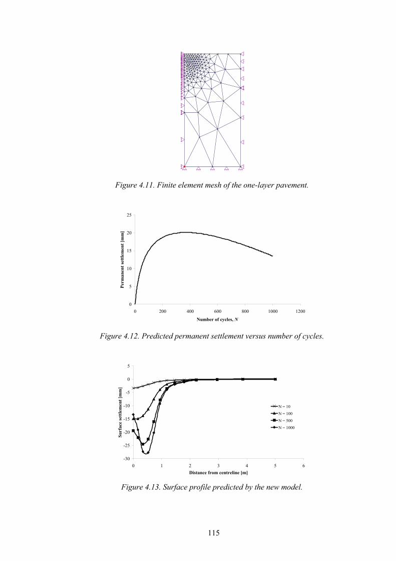
Figure 4.11. Finite element mesh of the one-layer pavement.

0

5

10

15

20

25

0 200 400 600 800 1000 1200

Number of cycles, N

Perm

anen

t set

tlem

ent [

mm

]

Figure 4.12. Predicted permanent settlement versus number of cycles.

-30

-25

-20

-15

-10

-5

0

5


Surf

ace

sett

lem

ent [

mm

]

N = 10

N = 100

N = 500

N = 1000

Figure 4.13. Surface profile predicted by the new model.

115

-10

-8

-6

-4

-2

0

2

0 200 400 600 800 1000 1200

Number of cycles, N

ε q [

%]

Figure 4.14. Accumulation of negative shear strain with number of cycles in

pavement element.

4.3.8 Modification of the Hardening Modulus

It has been shown in the previous section that the problem of accumulation of

negative shear strain occurs in the pavement analysis. This is due to the fact that the

shear strain decrement on unloading is greater than the increment during loading

under some stress conditions. As already discussed in Section 3.4.2, the negative

shear strain problem can be eliminated by modifying the hardening modulus such

that the stiffness on unloading is greater. In this section, the hardening modulus is

modified slightly in order to give a realistic prediction for the analysis of a

pavement.

Several modifications to the hardening moduli H1 and H2 were made in order to try

to eliminate the negative shear strain problem, such as using different values of ψ in

these terms (i.e. ψ1 in H1 term and ψ2 in H2 term), using 2p'o instead of p'o as the

scaling parameter in these terms, introducing the term p'c/p' into these terms, and

using different values of k in extension and compression according to equation 4.40.

None of these modifications eliminate the accumulation of negative shear strain

problem in the pavement analysis. Therefore a better modification is proposed

below.

116

For the two-surface model, Al-Tabbaa (1987) assumed that the hardening modulus, h is

expressed in the following form:

oh Fh H= + (4.42)

where F and H are scalar quantities which may be functions of stress state. For both

the two-surface model and the 3-SKH model the function F = 1. The negative shear

strain problem is due to the low stiffness on unloading; therefore the simplest way to

solve this problem is to increase the stiffness on unloading. The hardening modulus,

h, is expressed in the following form:

( )1 2oh F h H H= + + (4.43)

( )

144

4 4

21 1 sin 3

F αα α θ

= + + −

(4.44)

eFα = (4.45)

where Fe is the value of F in triaxial extension (θ = +30°). With this additional

function, F, the modulus on unloading can be adjusted whereas the modulus on

loading will remain unchanged.

A pavement problem was analysed using the new model with the value of k varying

according to equation 4.40, and using the function F according to equation 4.44.

Figure 4.15 shows the shear strain of the element located at the top of the subgrade

near the centreline (see Figure 4.15) as a function of number of cycles predicted by

these two models. Note that the equivalent stress blocks at the top of the subgrade

had to be calculated for each model. It can be seen that the negative shear strain

problem still exists when k is made to be a function of Lode angle according to

equation 4.40, with kc = 1.1 and ke = 0.5. Comparing Figure 4.14 with Figure 4.15,

the negative shear strain problem was slightly improved by using equation 4.40.

However, a more realistic prediction was obtained by using the function F for the

117

hardening modulus in equation 4.44. Therefore, it was considered that the

introduction of the function F in the hardening modulus was more appropriate.

-6

-4

-2

0

2

4


ε q [%

]

F varies according to equation 4.44 with F e = 3

k varies as in equation 4.40, with k c = 1.1 and k e = 0.5

Figure 4.15. Predicted shear strain as a function of number of cycles.

4.3.9 Determination of Parameters

Ten parameters are now required to fully describe the new model:

ecs – The voids ratio at p' = 1kPa on the critical state line.

M – The slope of the critical state line in q − p' space.

-λ* – The slope of the isotropic normal compression line and critical state line in ln v

− ln p' space.

-κ* – The initial slope of the swelling lines in ln v − ln p' space.

Ge – The elastic shear modulus.

T – The ratio of the size of the history surface to that of the bounding surface.

S – The ratio of the size of the yield surface to that of the history surface.

ψ – The exponent in the hardening moduli H1 and H2.

k – The parameter which controls the shape of the plastic potential.

Fe – The value of the multiplier in the hardening modulus in triaxial extension.

If the shear modulus is assumed to be dependent on the mean normal effective stress

p' and Ro according to equation 3.7, three extra parameters, A, n and m are needed.

118

However, these can be determined approximately if the plasticity index of the soil is

known (Viggiani and Atkinson, 1995).

The determination of the parameters for the 3-SKH model was described in Chapter

3. The additional parameter k for the new model is chosen such that the value of K0

during normally compression is correctly predicted. This can be determined by

neglecting elastic strains in the stress-dilatancy rule for one-dimensional conditions

as discussed in Section 4.3.7. For soils that satisfy the Jâky (1944) equation 2.37, the

parameter k can be determined from equation 4.39.

This serves as a guide to choosing the value of the new parameter k, and if equation

4.39 is being used, this means that only one extra parameter, Fe, is needed for the

new model.

The parameter Fe is determined by trial and error. It is shown in Chapter 5 that the

parameter Fe is suitable for modelling cyclic loading data, and in Chapter 6, it is

shown that the introduction of the parameter Fe leads to more realistic modelling of

pavement response.

4.4 SUMMARY

A new flow rule has been proposed in this chapter. With one additional parameter, k,

a family of plastic potentials can be obtained. The formulation of a three-surface

kinematic hardening model based on this flow rule has been presented. This new

non-associated three-surface kinematic hardening model is an extension of the 3-

SKH model (Stallebrass, 1990), which itself is an extension of the ‘Bubble’ model

(Al-Tabbaa, 1987). By choosing a suitable value of k, more realistic predictions of

shear strain and K0,nc can be obtained. These are over-predicted by the 3-SKH model

(Stallebrass, 1990). The simple non-associated flow rule is able to scale down the

plastic shear strain by a factor of k/2, and still gives associated flow under isotropic

conditions and at a critical state. The value of K0 on unloading can also be correctly

predicted if the value of the critical state parameter M is made to be a function of

119

Lode angle. If required, the value of parameter k could be permitted to be different

under compression and extension conditions. The value of the parameter k required

to correctly predict the value of K0 during normal compression may be determined

by trial and error, or it can be obtained by ignoring elastic strains in the stress-

dilatancy rule for one-dimensional normal compression. The new model was

implemented into a finite element code and triaxial simulations were performed and

it was shown that the prediction of shear strain and K0 during normal compression

and unloading were improved, although there is still some error on reloading: this is

a function of H1 and H2 and is due to the strong ratcheting phenomenon exhibited by

the model. The prediction of the value of K0 on reloading by the 3-SKH model is

better than the new model, but this is mainly because of the higher value of K0,nc. As

for the 3-SKH model, the new model also suffers from the problem of accumulation

of negative shear strain under some stress conditions where the hardening modulus

on unloading is not large enough. However, this can be eliminated by modifying the

hardening modulus, h. The hardening modulus was modified such that it would

become larger on unloading by introducing a scaling factor Fe. This is examined in

detail in Chapter 5.

120

5 EXPERIMENTAL VALIDATION OF THE NON-

ASSOCIATED THREE-SURFACE KINEMATIC

HARDENING MODEL

5.1 INTRODUCTION

A new non-associated three-surface kinematic hardening model was proposed in the

previous chapter. In this chapter, the model parameters for kaolin clay are

determined by triaxial testing using the methods proposed by Stallebrass (1997) –

see Section 3.2.3. Drained cyclic loading tests were performed to validate the model

and to determine the parameters ψ, and Fe, that best fit the data. Due to time

constraints caused by the difficulties in the commissioning of the equipment, only

two drained cyclic loading tests were performed. Each test took approximately five

weeks to complete.

5.2 TRIAXIAL TEST

This section briefly describes the triaxial apparatus used, the sample preparation, and

the procedure followed in performing the tests. The GDS advanced triaxial testing

system was used in this research. A detailed description of the triaxial apparatus can

be found in Menzies (1988) and the GDS Laboratory manual (GDS Instruments Ltd,

2002). All of the tests reported here were performed on samples of Speswhite kaolin

prepared by mixing Speswhite kaolin powder with distilled water at a water content

of 130% and then consolidating in an oedometer. The test results are reported and

discussed in this chapter.

121

5.2.1 Description of the Triaxial Apparatus

The GDS triaxial testing system was used for this research to carry out the necessary

triaxial testing. A brief description of this system is given in this section.

The system consists of a triaxial cell, two standard and one advanced computer

controlled pressure sources, an eight-channel data acquisition pad, a computer and a

multiplexer which allows up to four devices to be connected to a communication

port on the computer. The system layout is shown in Figure 5.1.

Figure 5.1. Schematic diagram showing the layout of the triaxial system (GDS

Instruments Ltd, 2002).

Triaxial cell

The triaxial cell is a Bishop and Wesley (1975) cell which has a maximum safe

working pressure of 1700kPa. Both 38mm and 50mm diameter specimens can be

tested using this cell. Axial force is exerted on the test specimen by a piston fixed to

the base pedestal. This piston moves vertically upwards and downwards actuated

hydraulically from the lower chamber in the base of the cell, which contains water.

Known displacements may be applied by pumping a known volume of water from a

GDS pressure controller into the lower chamber. GDS standard pressure/volume

controllers are used to control both the lower chamber pressure and the cell pressure.

A 2kN internal submersible load cell which has an accuracy of 2N, one external

122

axial displacement transducer with a range of 40mm and an accuracy of 0.1mm, and

one 2000kPa range pore pressure transducer with an accuracy of 2kPa are used. The

back pressure is applied to the top of the sample by a GDS advanced

pressure/volume controller and the volume change of the sample is also measured by

this controller. The pore pressure is measured at the base of the sample. The

measurement of local strain is discussed later.

Pressure/volume controller

The triaxial system consists of three 2MPa pressure/volume controllers: two standard

pressure/volume controllers to control the cell pressure and lower chamber pressure

and one advanced pressure/volume controller for the back pressure source. The

volumetric capacity of these controllers is 2×10-4m3. The resolution of the pressure

control is 2kPa and the resolution of pressure measurement is 1kPa.

Hall effect transducers

If current is flowing through a semiconductor plate that is placed in a magnetic field

where flux lines are directed perpendicular to both the material and the current flow,

voltage is produced across the plate in a direction normal to the current flow. This is

known as the Hall effect. The application of Hall effect transducers to measure local

axial and radial deformation in the triaxial test has been successfully performed at

the University of Surrey (Clayton et al., 1989). The radial strain-measuring device

consists of a calliper, which is mounted on the test specimen by pins or bonded to the

membrane by adhesive. The Hall effect transducer is positioned across the opening

at the calliper where it measures the opening and closing of the jaws. Figure 5.2

shows the radial strain-measuring device mounted on the test specimen. For axial

strain measurement, the device consists of a spring-mounted pendulum that holds a

magnet assembly, which is suspended from a mounting block. This mounting block

is fixed to the test specimen by pins or bonded to the membrane by adhesive. The

lower part of the transducer, which is mounted on the specimen by pins or adhesive,

consists of a metallic container holding the linear output Hall effect semiconductor.

The range of the Hall effect transducer is ±3mm with an accuracy of 0.05mm; at this

123

range the output of the transducer is almost linear. The Hall effect transducers were

used in all the triaxial tests performed.

Radial calliper Hall effect transducer

Local axial measurement Soil sample

Figure 5.2. Picture showing the on-sample instrumentation.

5.2.2 Soil Used in the Experimental Test

The soil used in this research is Speswhite kaolin provided in dry powder form. The

soil sample was prepared by mixing the kaolin powder with distilled water of twice

the liquid limit and consolidating in an oedometer. Index tests were performed to

determine the liquid limit and plastic limit. The liquid limit and plastic limit were

found to be 63% and 31% respectively. Other researchers have obtained similar

value for Speswhite kaolin. The liquid limit and plastic limit obtained by Atkinson

(1987) were 65% and 35% respectively, by Al-Tabbaa (1987) 69% and 38%

respectively, and by Martin & Houlsby (2000) 65% and 34% respectively.

5.2.3 Sample Preparation

A 100mm diameter oedometer was used to prepare samples for triaxial testing.

Figure 5.3a shows the base, top cap and porous stones for the oedometer. Sufficient

amount of dry Speswhite kaolin powder was mixed with distilled water at a moisture

124

content of 130% (twice the liquid limit) to form the slurry. The slurry was then

poured into the oedometer with care to ensure that no air was trapped. Filter paper

was soaked in water and placed on the top and bottom porous stones so that clay

would not clog them. Drainage was allowed at the top and bottom. The vertical

pressure was applied using a pressure regulator which had been calibrated against a

load cell. A photograph of the oedometer in use is shown in Figure 5.3b. The kaolin

slurry was one-dimensionally consolidated to a vertical pressure of 200kPa. This

pressure was applied in increments of 10, 20, 50, 100, and 200kPa. Each increment

of pressure was held for a period of at least 48 hours to allow the excess pore

pressure to dissipate. The sample was then unloaded to 100kPa and the sample was

left under this pressure until extrusion. This would leave the sample in an

approximately isotropic state of p' ≈ 100kPa (Al-Tabbaa, 1987) which could then be

easily recreated in the triaxial cell. The whole process took approximately three

weeks. During extrusion, a thin wire was run along the circumference of the sample

to reduce the friction between the soil specimen and the oedometer when it was

being pushed out. The sample was then trimmed to the required size using a wire

saw and a trimming apparatus. During the process of extrusion and trimming, great

care was taken in order to keep the sample disturbance to a minimum. Initial

dimensions, weight and moisture content of the specimen were measured before

setting up the specimen in the triaxial apparatus.

(a) (b)

Figure 5.3. (a) Oedometer, porous stones, top and base caps, and (b) sample under

one-dimensional consolidation.

125

5.2.4 Specimen Set Up and Test Procedure

After the sample was trimmed to the required dimensions, in this case a diameter of

38mm and height 76mm, the specimen was ready to be set up in the triaxial

apparatus. Before the specimen was set up in the triaxial apparatus, the pore pressure

line was de-aired by flushing it with water and the reading of the pore pressure was

set to zero. A porous stone which had been soaked overnight was slid over a layer of

water on the base pedestal without trapping any air. Filter paper and the specimen

were then placed on the porous stone. The second filter paper and porous stone were

then placed on top of the specimen. After that, three filter strips of ¾ of the length of

the sample were placed on the side of the specimen for side drainage. For the

extension test, fishnet spiral filter strips were used in order to minimise the stiffness

of the filter paper. After that, a rubber membrane was put onto the sample using a

membrane stretcher. A vacuum was applied to the membrane stretcher to help put

the membrane on. A de-aired top cap was then placed on top of the sample. Two O-

rings were used for each end to seal the membrane to the base pedestal and the top

cap. The Hall effect transducers were installed at this stage. For triaxial extension, a

vylastic sleeve and an extension top cap were used. The vylastic sleeve was smeared

with a layer of silicone grease to prevent leakage. The triaxial cell was then

assembled, and the load cell reading set to zero. The cell was filled with water with

the air bleed open. When the water level reached the mid height of the sample, the

cell and lower chamber pressure readings were set to zero. The load cell was lowered

slowly until it just made contact with the top cap. When the extension top cap was

used, a very small vacuum was applied to ensure contact between the top cap and the

extension cap. When the cell was completely filled with water the air outlet valve

was closed and the specimen was ready for testing. Initially, a cell pressure of 50kPa

was applied with the drainage valve closed. This was to measure the initial effective

stress of the sample. The pressure was held for a period of time until pore pressure

stabilized, and the effective stress was noted. After that, the drainage valve was

opened and back pressure saturation was performed by applying back pressure and

cell pressure simultaneously and incrementally to keep the effective stress

unchanged. The back pressure used was about 430kPa for all the tests and the B-

126

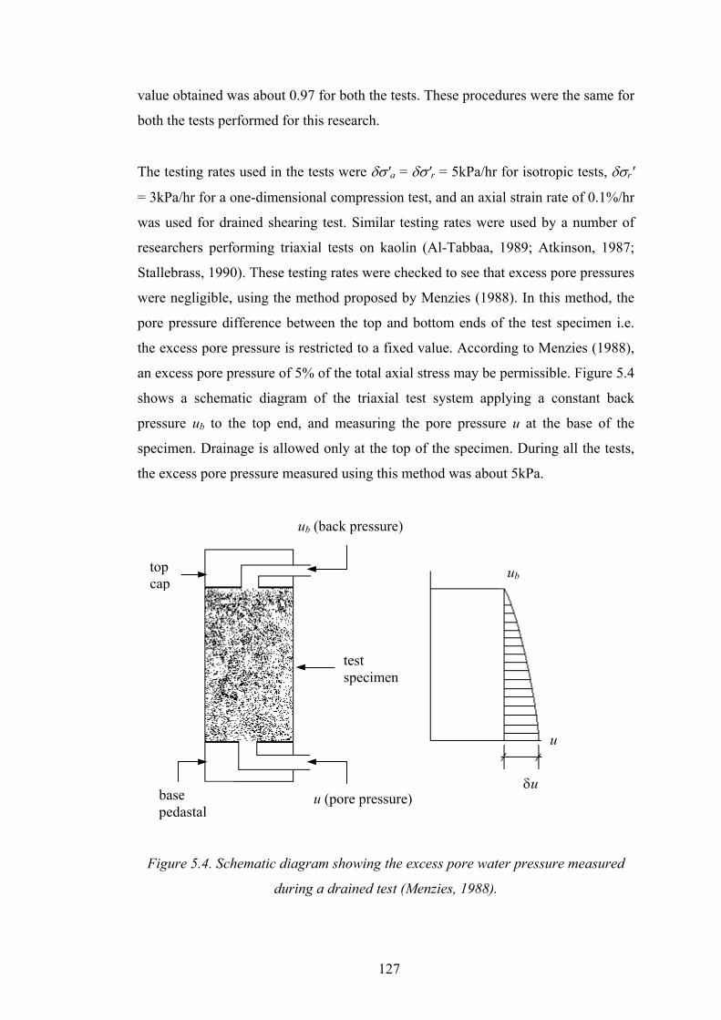
value obtained was about 0.97 for both the tests. These procedures were the same for

both the tests performed for this research.

The testing rates used in the tests were δσ'a = δσ'r = 5kPa/hr for isotropic tests, δσr'

= 3kPa/hr for a one-dimensional compression test, and an axial strain rate of 0.1%/hr

was used for drained shearing test. Similar testing rates were used by a number of

researchers performing triaxial tests on kaolin (Al-Tabbaa, 1989; Atkinson, 1987;

Stallebrass, 1990). These testing rates were checked to see that excess pore pressures

were negligible, using the method proposed by Menzies (1988). In this method, the

pore pressure difference between the top and bottom ends of the test specimen i.e.

the excess pore pressure is restricted to a fixed value. According to Menzies (1988),

an excess pore pressure of 5% of the total axial stress may be permissible. Figure 5.4

shows a schematic diagram of the triaxial test system applying a constant back

pressure ub to the top end, and measuring the pore pressure u at the base of the

specimen. Drainage is allowed only at the top of the specimen. During all the tests,

the excess pore pressure measured using this method was about 5kPa.

ub (back pressure)

ub

top cap

test specimen

u

base pedastal

δu u (pore pressure)

Figure 5.4. Schematic diagram showing the excess pore water pressure measured

during a drained test (Menzies, 1988).

127

5.2.5 Analysis of Data

The test results were interpreted in terms of the deviatoric stress q = (σ'a − σ'r) and

the effective mean normal stress p' =(σ'a+2σ'r)/3, where σ'a and σ'r are the axial and

radial effective stresses respectively. The corresponding strains were shear strain εq =

2(εa−εr)/3 and volumetric strain εp = εa + 2εr, where εa and εr are the axial and radial

strains respectively. Following Stallebrass (1990), all the strains used were true

strains calculated from the engineering strains as these strains eliminate errors when

strains become large and are more appropriate for comparison with incremental

constitutive soil models. The axial strain is defined as:

(d ln 1ol

a l

ll

)oε ε= = − −∫ (5.1)

where compressive strain is positive, lo is the initial height l is the current height, and

εo is the engineering strain:

oo

llδε = (5.2)

5.3 DETERMINATION OF MODEL PARAMETERS

In this section, the results which were used for determination of parameters are

presented. There are ten parameters required to define the new model; five of which

are Modified Cam clay parameters, plus the parameters to define the size of the

kinematic surfaces, T and S, the parameter ψ, and the new parameters k, and Fe. The

method described by Stallebrass (1997) was used to obtain the required parameters

and this has been described briefly in Section 3.2.3. For this purpose, the bulk

stiffness K' = δp'/δεp was calculated by fitting a straight line to data points on the

graph of p' versus εp over a stress change of approximately 15kPa (Stallebrass,

1990). The new parameter k was obtained from a one-dimensional normal

compression test and the parameters ψ and Fe were determined by fitting the cyclic

loading test results.

128

5.3.1 Model Parameters

(i) Modified Cam clay model parameters

Figures 5.5 and 5.6 shows the isotropic normal compression and swelling lines in v –

ln p' space and ln v – ln p' space respectively for a test performed on a specimen of

Speswhite kaolin. The slopes of the normal compression line in v – ln p' space and ln

v – ln p' space are denoted by -λ and -λ* respectively. The values for λ and λ* were

found to be 0.19 and 0.073 respectively, and the isotropic line is fixed at the point p'

= 400kPa and v = 2.071.

Following Stallebrass (1990), by plotting K'/p' against p'/p'm (p'm is the maximum

mean effective pressure to which the soil has been loaded) for isotropic swelling

from a normally consolidated state, the value of κ* can be estimated as the initial

value of p'/K'. The value of κ* is not very reliable because measuring stiffness at

very small strains is difficult. Figure 5.7 shows the result for K'/p' versus p'/p'm. The

parameter κ* was determined from the initial part of the curve with p'/p'm = 1, and

was found to be 0.003. For a linear isotropic normal compression line in v – ln p'

space, the value of v at 1kPa, denoted by N, would be 3.209. This gives the critical

state void ratio ecs, at p' = 1kPa a value of ecs = 2.056 (ecs can be calculated from

ln(1+ecs)= ln N – (λ*–κ*) ln 2).

2.0

2.1

2.2

2.3

2.4

2.5

2 3 4 5 6 7

ln p'

v

Figure 5.5. Isotropic normal compression line and swelling line in v – ln p' space.

129

0.70

0.75

0.80

0.85

0.90

2 3 4 5 6 7

ln p'

ln v

Figure 5.6. Isotropic normal compression line and swelling line in ln v – ln p' space.

0

50

100

150

200

250

300

350

400

0.0 0.2 0.4 0.6 0.8 1.0

p' /p' m

K'/ p

'

Figure 5.7. Result showing K'/p' versus p'/p'm during isotropic unloading.

The critical state dissipation constant, M, was obtained from a strain-controlled

drained shearing test at 0.1%/hr with constant cell pressure. A critical state is said to

have been reached when the soil undergoes large deviatoric strains at constant stress

ratio, and at constant volume. The results for stress ratio versus shear strain, and

volumetric strain versus shear strain are presented in Figures 5.8 and 5.9

respectively. A clearly defined critical state has been reached at a stress ratio M =

0.86 after a deviatoric strain εq ≈ 18%. This value of M corresponds to a friction

angle φ' = 22°.

130

The elastic shear modulus was estimated from the relationship proposed by Viggiani

and Atkinson (1995) – see Equation 3.7. The coefficients A, m, and n can be

obtained from Figure 5.10 produced by Viggiani and Atkinson (1995) if the

plasticity index is known. These charts were derived from test data for different soil

types with different plasticity indices. The coefficients A, m, and n obtained by

Viggiani and Atkinson (1995) for Speswhite kaolin clay were 1964, 0.2, and 0.65.

However, the plasticity index of their soil was 24%, which is smaller than the value

obtained in this present study (PI = 32%). From Figure 5.10, for soil with PI = 32%

the coefficients A, m, and n are approximately 1,000, 0.8, and 0.24 respectively.

Figure 5.11 shows the effect of these parameters on the prediction of permanent

settlement in a pavement problem. The resilient deformations predicted using the

coefficients obtained by Viaggiani & Atkinson (1995) and from Figure 5.10 with PI

= 32% were 0.26mm and 0.25mm respectively. In addition, the results in Figure 5.11

show that the values of these parameters have no significant influence on the

predicted permanent deformations. Hence, the coefficients used by Stallebrass

(1997) will be used since they have been well established by bender element tests.

0.0

0.1

0.2

0.3

0.4

0.5

0.6

0.7

0.8

0.9

1.0

0 5 10 15 20ε q [%]

q/ p

'

Figure 5.8. Deviatoric stress-strain curve for a conventional drained triaxial test.

131

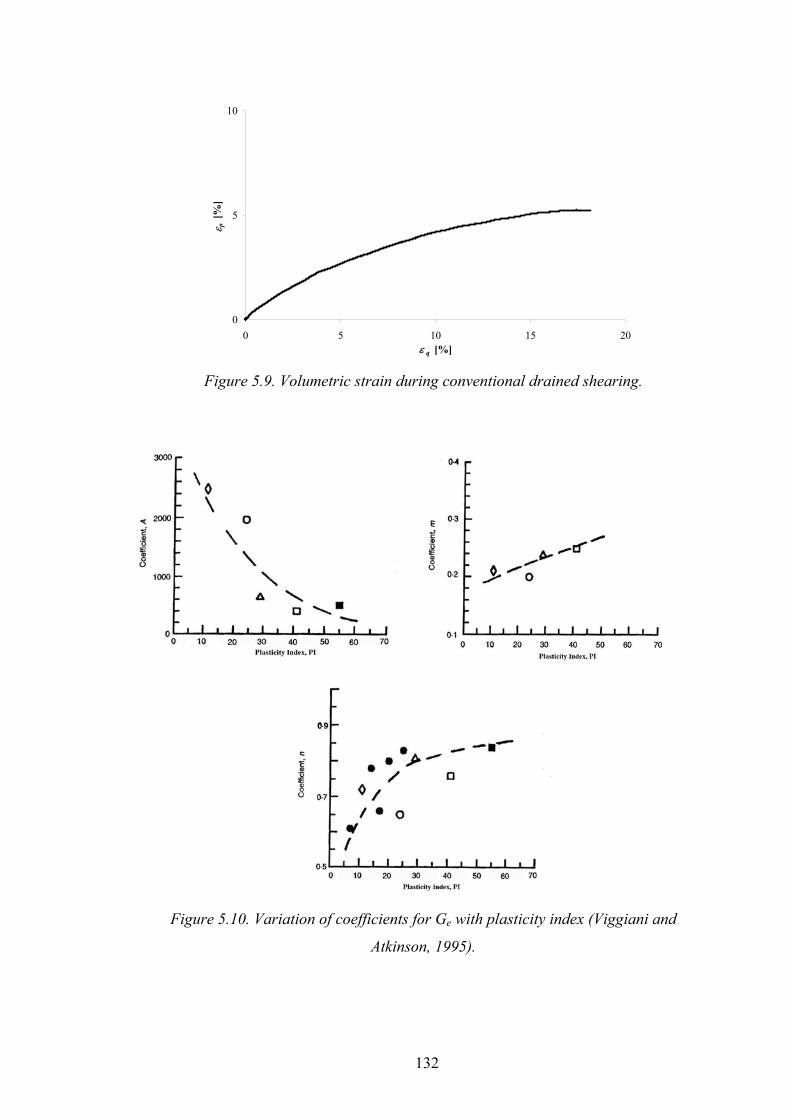
0

5

10

0 5 10 15 20ε q [%]

ε p [%

]

Figure 5.9. Volumetric strain during conventional drained shearing.

Figure 5.10. Variation of coefficients for Ge with plasticity index (Viggiani and

Atkinson, 1995).

132

0

5

10

15

20

25

0 200 400 600 800 1000 1200N

Perm

anen

t set

tlem

ent [

mm

]A = 1964, m = 0.2, n = 0.65

A = 1000, m = 0.24, n = 0.8

Figure 5.11. Effect of parameters A, m, and n on the predicted permanent settlement

of a three-layer pavement.

(ii) T and S

The parameters T and S that determine the size of the history and the yield surfaces

were determined by isotropic unloading and reloading as described by Stallebrass

(1997), see Section 3.2.3. The stress path followed in this test is shown in Figure 3.6

with p' = p'm = 510kPa (point O), followed by swelling back to p' = 250kPa (point

B). Figures 5.12 presents the results of the bulk stiffness versus change in stress for

stress paths with angles of stress rotation, ϕ = 0° and ϕ = 180°. To determine the

parameter T, the stress change, ∆p' = 2Tp'o at which the two stiffness curves meet, is

obtained from Figure 5.12. From the data presented in this figure, there is not a well-

defined point where the two stiffness curves meet. Inspection of Figure 5.12 shows

that the stiffness curves merge at approximately ∆p' = 140kPa, which gives T a value

of approximately 0.27. The very small strain stiffness, which is needed to determine

the size of the elastic region, cannot easily be measured using a triaxial apparatus, as

the very small strain stiffness usually occurs at strain levels below 0.001%

(Atkinson, 2000). The stiffness at this strain level is usually measured using bender

elements or a resonant column; unfortunately these devices were not available for

this research. So based on this study and that of Stallebrass (1990), values of T =

0.25 and S = 0.08 might be appropriate. It will be shown that these values are

appropriate for modelling behaviour under cyclic loading.

133

0

20,000

40,000

60,000

80,000

100,000

120,000

140,000

0 20 40 60 80 100 120 140 160 180

∆p' [kPa]

K'

[kPa

]

ϕ = 180o

ϕ = 0o

Figure 5.12. Curves showing the variation in bulk stiffness with ∆p' for stress

rotations ϕ = 0° and ϕ = 180°.

(iii) k

The new parameter, k, which determines the shape of the plastic potential and hence

the value of K0,nc, can be obtained from a one-dimensional normal compression test.

Figure 5.13 shows the results of K0,nc versus εa during a one-dimensional loading

test. The value of K0,nc reached a constant value of 0.72 (η0,nc = 0.344) at axial strain

of approximately 14%. Al-Tabbaa (1987) obtained a K0,nc value of 0.69 for her test

on kaolin. By neglecting elastic strains, the parameter k can be estimated, given the

friction angle φ' and the value of K0,nc. The value of k corresponding to φ' = 22° (M =

0.86) and K0,nc = 0.72 (η0,nc = 0.344) is 1.2, according to equation 4.38 (i.e. ignoring

elastic strains) or Figure 4.7.

0.0

0.2

0.4

0.6

0.8

1.0

1.2

0 2 4 6 8 10 12 14

ε a [%]

K0

16

Figure 5.13. Experimental data showing K0 values versus axial strain, εa.

134

All the model parameters can be determined directly, except ψ and Fe which can

only be determined by trial and error (i.e. parametric studies). However, the values

of T, S, and κ*, cannot be measured very accurately, as discussed. Consequently,

parametric studies have been performed using cyclic loading data to determine the

parameters ψ, and Fe, and better estimates of the parameters T, S, and κ*, suitable for

modelling cyclic loading. This is described in the next section.

5.3.2 Parametric Study

The purpose of this study was to determine the parameters ψ and Fe that best fit

experimental data and to make better estimates of the parameters T, S, and κ* for the

purpose of modelling behaviour under cyclic loading. The effect of the parameters ψ

and Fe will first be investigated (these can only be determined by trial and error):

before continuing to investigate the effects of other parameters, sensible values of

these parameters are required. This is followed by an investigation of the influence

of parameters T, S, and κ*. The rest of the parameters were unchanged during these

simulations. The values were M = 0.86, λ* = 0.073, k = 1.2, and Ge varied according

to equation 3.7 with A = 1964, m = 0.2, and n = 0.65.

For this parametric study, the stress-strain behaviour of a conventional drained cyclic

test on Speswhite kaolin was simulated and compared with the experimental data.

The recent stress histories of the sample were simulated in the finite element

modelling. The drained cyclic test was performed using the same sample that had

been used for the determination of the model parameters T and S. After the isotropic

stress reversal (ϕ = 180°) for the determination of the stiffness curve, the sample was

isotropically compressed to p' = 545kPa and a cyclic stress ratio was applied at a

constant cell pressure between η = 0 and η = 0.2. Figure 5.14 presents the stress-

strain curves for the test.

135

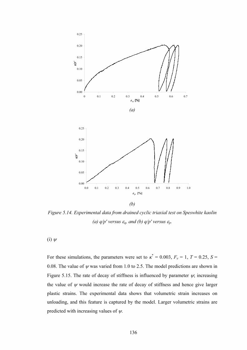
0.00

0.05

0.10

0.15

0.20

0.25

0 0.1 0.2 0.3 0.4 0.5 0.6 0.7ε q [%]

q/p'

(a)

0.00

0.05

0.10

0.15

0.20

0.25

0.0 0.1 0.2 0.3 0.4 0.5 0.6 0.7 0.8 0.9 1.0

ε p [%]

q/p'

(b)

Figure 5.14. Experimental data from drained cyclic triaxial test on Speswhite kaolin

(a) q/p' versus εq, and (b) q/p' versus εp.

(i) ψ

For these simulations, the parameters were set to κ* = 0.003, Fe = 1, T = 0.25, S =

0.08. The value of ψ was varied from 1.0 to 2.5. The model predictions are shown in

Figure 5.15. The rate of decay of stiffness is influenced by parameter ψ; increasing

the value of ψ would increase the rate of decay of stiffness and hence give larger

plastic strains. The experimental data shows that volumetric strain increases on

unloading, and this feature is captured by the model. Larger volumetric strains are

predicted with increasing values of ψ.

136

0.00

0.05

0.10

0.15

0.20

0.25

0 0.2 0.4 0.6 0.8 1 1.2 1.4ε q [%]

q/ p

'ψ = 1.0

ψ = 2.0

ψ = 1.5

ψ = 2.5

(a)

0.00

0.05

0.10

0.15

0.20

0.25

0 0.2 0.4 0.6 0.8 1 1.2 1.4 1.6ε p [%]

q/ p

'

ψ = 1.0ψ = 1.5ψ = 2.0ψ = 2.5

(b)

Figure 5.15. Effect of ψ on the stress-strain behaviour (a) q/p' versus εq, and (b) q/p'

versus εp.

(ii) Fe

By comparing the results presented in Figures 5.14 and 5.15, the value ψ =1.5 was

chosen to investigate the effect of the parameter Fe (ψ = 2 could have been chosen,

but this gives too much shear strain on first loading). The rest of the parameters are

the same as in the above parametric study of parameter ψ. The parameter Fe was

varied from 1 to 4 and the effect of this parameter on the stress-strain curves is

illustrated in Figure 5.16. As can be seen from this figure, the volumetric strain is

137

relatively insensitive to the variation of the parameter Fe. Increasing the value of Fe

increases the stiffness on unloading and hence smaller strains are recovered on

unloading. The predicted total shear strains are larger with a larger value of Fe.

0.00

0.05

0.10

0.15

0.20

0.25

0 0.1 0.2 0.3 0.4 0.5 0.6 0.7 0.8

ε q [%]

q/ p

'

F e = 4F e = 3

F e = 1F e = 2

(a)

0.00

0.05

0.10

0.15

0.20

0.25

0 0.2 0.4 0.6 0.8 1 1.2 1.4

ε p [%]

q/ p

'

F e = 1

F e = 2

F e = 3F e = 4

(b)

Figure 5.16. Effect of Fe on the stress-strain behaviour (a) q/p' versus εq, and (b) q/p'

versus εp.

(iii) κ*

The influence of κ* on the stress-strain curves is shown in Figure 5.17. The value of

κ* was varied from 0.003 to 0.007 and by comparing Figures 5.14 and 5.16, the

value Fe = 3 was chosen in this parametric study. Increasing the value of κ* leads to

138

the accumulation of smaller plastic strains. A value of κ* = 0.003 was found to fit the

data quite well.

0.00

0.05

0.10

0.15

0.20

0.25

0 0.1 0.2 0.3 0.4 0.5 0.6 0.7ε q [%]

q/ p

'

κ ∗ = 0.003

κ ∗ = 0.005

κ ∗ = 0.007

(a)

0.00

0.05

0.10

0.15

0.20

0.25

0 0.2 0.4 0.6 0.8 1 1.2 1.4ε p [%]

q/ p

'

κ ∗ = 0.003

κ ∗ = 0.005

κ ∗ = 0.007

(b)

Figure 5.17. Effect of κ* on the stress-strain behaviour (a) q/p' versus εq, and (b) q/p'

versus εp.

(iv) TS

This section investigates the effect of the size of the elastic region on the stress-strain

behaviour. The size of the elastic region was varied from TS = 0.01 to TS = 0.03 with

the size of the history surface (i.e. T) unchanged. The parameters were set to κ* =

0.003, Fe = 3, ψ = 1.5, and T = 0.25. The results are shown in Figure 5.18. It can be

139

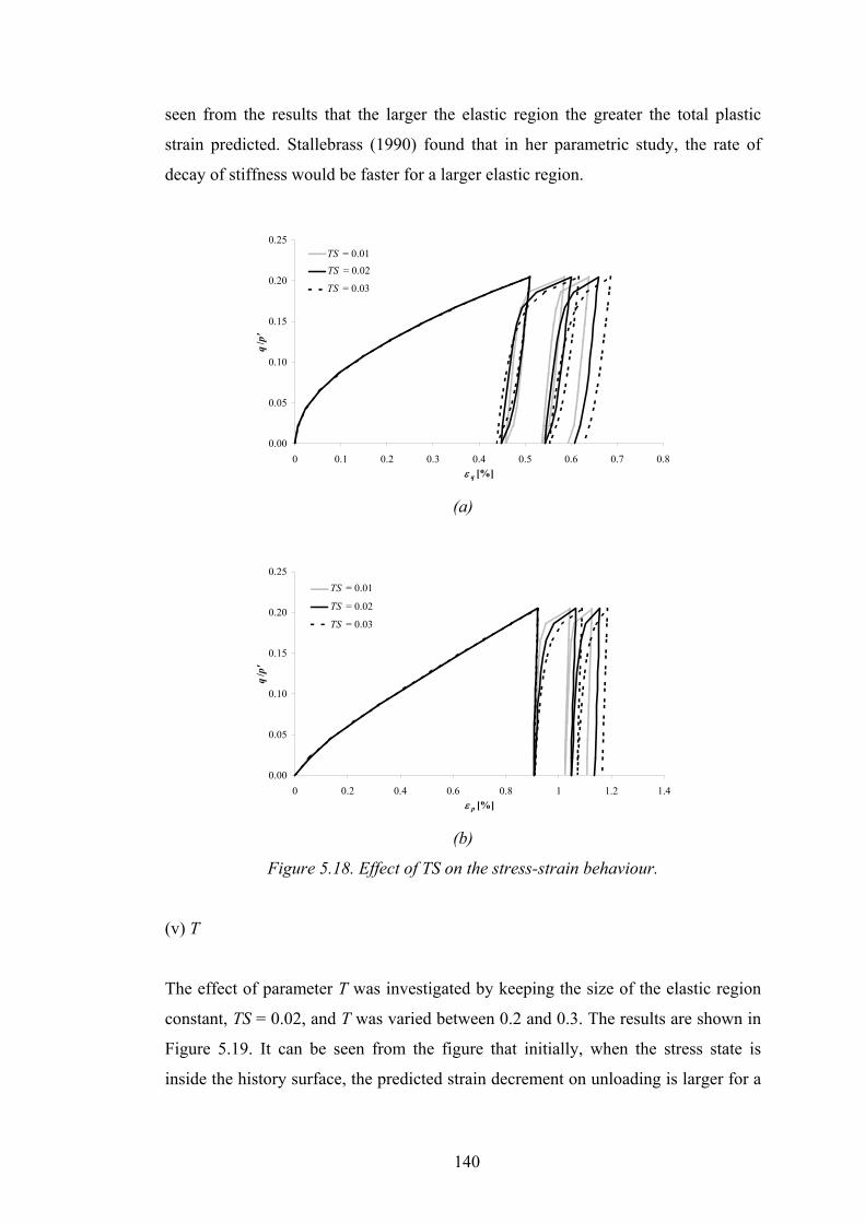
seen from the results that the larger the elastic region the greater the total plastic

strain predicted. Stallebrass (1990) found that in her parametric study, the rate of

decay of stiffness would be faster for a larger elastic region.

0.00

0.05

0.10

0.15

0.20

0.25

0 0.1 0.2 0.3 0.4 0.5 0.6 0.7 0.8ε q [%]

q/ p

'TS = 0.01TS = 0.02

TS = 0.03

(a)

0.00

0.05

0.10

0.15

0.20

0.25

0 0.2 0.4 0.6 0.8 1 1.2 1.4ε p [%]

q/ p

'

TS = 0.01

TS = 0.02

TS = 0.03

(b)

Figure 5.18. Effect of TS on the stress-strain behaviour.

(v) T

The effect of parameter T was investigated by keeping the size of the elastic region

constant, TS = 0.02, and T was varied between 0.2 and 0.3. The results are shown in

Figure 5.19. It can be seen from the figure that initially, when the stress state is

inside the history surface, the predicted strain decrement on unloading is larger for a

140

smaller history surface as stiffness decays more quickly. The total strain accumulated

increases with decreasing size of the history surface.

0.00

0.05

0.10

0.15

0.20

0.25

0 0.1 0.2 0.3 0.4 0.5 0.6 0.7 0.8 0.9ε q [%]

q/ p

'

T = 0.20

T = 0.25T = 0.30

(a)

0.00

0.05

0.10

0.15

0.20

0.25

0 0.2 0.4 0.6 0.8 1 1.2 1.4 1.6ε p [%]

q/ p

'

T = 0.20

T = 0.25

T = 0.30

(b)

Figure 5.19. Effect of T on the stress-strain behaviour (a) q/p' versus εq, and (b) q/p'

versus εp.

For the range of values used in this parametric study for parameters κ*, T, and S, it

was found that κ* and the size of the yield surface (for a given T) have relatively

little influence on the stress-strain behaviour. For a given size of the yield surface TS,

the size of the history surface T has a much greater effect, and the parameter ψ also

has a considerable effect on the stress-strain behaviour. Generally the model is able

to fit the experimental data well, but the model slightly over-predicts volumetric

141

strain. The model can reproduce some of the features of soil under repeated loading

as observed in the experiments, such as the increase in volumetric strain during

unloading, and the gradual decrease of the strain increments with increasing number

of cycles.

From the comparison between the experimental data and the model predictions

shown in Figures 5.14 – 5.19, the model parameters that best represent Speswhite

kaolin were obtained. These were: M = 0.86, λ* = 0.073, κ* = 0.003, ecs = 2.056, A =

1964, m = 0.2, n = 0.65, T = 0.25, S = 0.08, k = 1.2, ψ = 1.5, and Fe = 3. These

parameters are used in all subsequent analyses presented in Chapters 5 and 6. The

comparison between the model predictions using these parameters and the

experimental data are presented in Figure 5.20.

0.00

0.05

0.10

0.15

0.20

0.25

0 0.1 0.2 0.3 0.4 0.5 0.6 0.7

ε q [%]

q/ p

'

Model prediction

Experimental data

(a)

0.00

0.05

0.10

0.15

0.20

0.25

0 0.2 0.4 0.6 0.8 1 1.2

ε p [%]

q/ p

'

1.4

Model prediction

Experimental data

(b)

Figure 5.20. Comparison of model predictions and experimental data (a) q/p' versus

εq, and (b) q/p' versus εp.

142

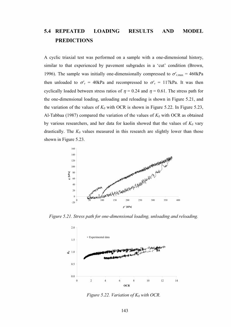
5.4 REPEATED LOADING RESULTS AND MODEL

PREDICTIONS

A cyclic triaxial test was performed on a sample with a one-dimensional history,

similar to that experienced by pavement subgrades in a ‘cut’ condition (Brown,

1996). The sample was initially one-dimensionally compressed to σ'v,max = 460kPa

then unloaded to σ'v = 40kPa and recompressed to σ'v = 117kPa. It was then

cyclically loaded between stress ratios of η = 0.24 and η = 0.61. The stress path for

the one-dimensional loading, unloading and reloading is shown in Figure 5.21, and

the variation of the values of K0 with OCR is shown in Figure 5.22. In Figure 5.23,

Al-Tabbaa (1987) compared the variation of the values of K0 with OCR as obtained

by various researchers, and her data for kaolin showed that the values of K0 vary

drastically. The K0 values measured in this research are slightly lower than those

shown in Figure 5.23.

-20

0

20

40

60

80

100

120

140

160

0 50 100 150 200 250 300 350 400

p' [kPa]

q [k

Pa]

Figure 5.21. Stress path for one-dimensional loading, unloading and reloading.

0.0

0.5

1.0

1.5

2.0

0 2 4 6 8 10 12 14

OCR

K0

Experimental data

Figure 5.22. Variation of K0 with OCR.

143

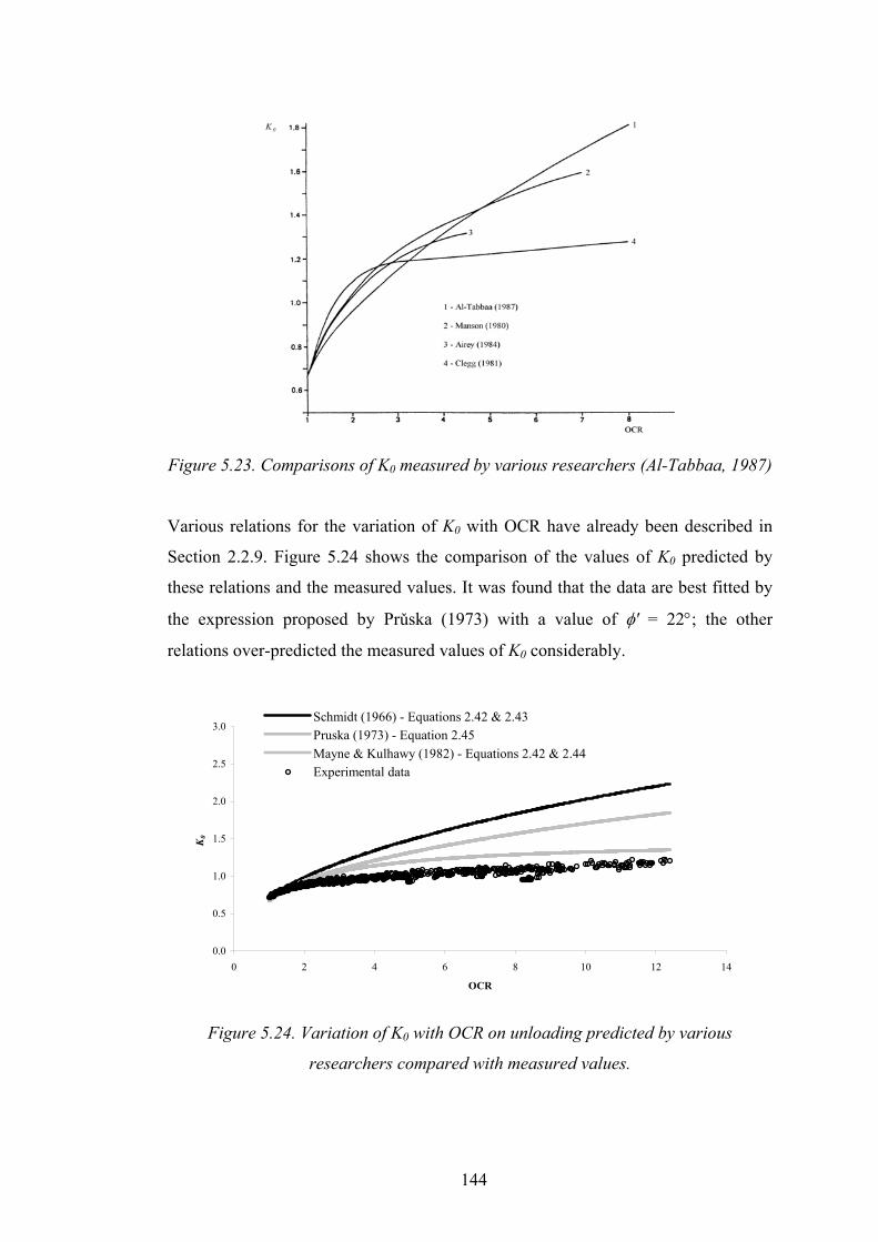
Figure 5.23. Comparisons of K0 measured by various researchers (Al-Tabbaa, 1987)

Various relations for the variation of K0 with OCR have already been described in

Section 2.2.9. Figure 5.24 shows the comparison of the values of K0 predicted by

these relations and the measured values. It was found that the data are best fitted by

the expression proposed by Prǔska (1973) with a value of φ' = 22°; the other

relations over-predicted the measured values of K0 considerably.

0.0

0.5

1.0

1.5

2.0

2.5

3.0

0 2 4 6 8 10 12 14

OCR

K0

Schmidt (1966) - Equations 2.42 & 2.43Pruska (1973) - Equation 2.45Mayne & Kulhawy (1982) - Equations 2.42 & 2.44Experimental data

Figure 5.24. Variation of K0 with OCR on unloading predicted by various

researchers compared with measured values.

144

The new model prediction of the variation the values of K0 with OCR on unloading

and reloading, is shown in Figure 5.25. Using a value of k = 1.2, the model predicts a

value of K0,nc of 0.714 (η0,nc = 0.353) compared to 0.72 measured from the triaxial

test and dεpp/dεq

p = 1.45. It can be seen that the model over-predicts K0 on both

unloading and reloading. This is because of the value of Fe and ψ chosen, which

make the stiffness on unloading higher, giving a higher value of K0. However, it

should be noted that the values of K0 measured are relatively lower compared to the

values of K0 obtained by other researchers. For pavement problems, it is more

important to be able to predict the behaviour of a clay subgrade under cyclic loading

than to predict the correct value of K0; therefore the model parameters have been

determined by fitting a set of cyclic loading data. If K0 is of interest, alternative

model parameters can be chosen.

0.0

0.5

1.0

1.5

2.0

2.5

3.0

0 2 4 6 8 10 12 14OCR

K0

Model prediction

Experimental data

Unloading

Reloading

Figure 5.25. Comparison of model prediction and experimental data.

Figures 5.26 and 5.27 show the cyclic test results and model predictions respectively.

It should be noted that for the triaxial simulation, the stress history is approximately

the same as that for the sample in the triaxial test, so that the yield surface and

history surface start off at the correct positions before cyclic loading. The predicted

shear strain after ten cycles is close to the measured value. However the model

predicts a strong ratcheting behaviour which is not observed experimentally. This

ratcheting problem will cause the rut depth to be over-estimated under large numbers

of cycles in a pavement analysis; this is shown later in Chapter 6. The shear strain

increments measured in the apparatus are decreasing with increasing number of

145

cycles whilst the shear strain increment after the first cycle predicted by the model

remains constant. It can be seen that from Figure 5.26, the volumetric strain was

compressive for the first cycle and became dilative. The model predicted the same

trend of behaviour but the actual predicted values of volumetric strain were more

dilative.

0

0.1

0.2

0.3

0.4

0.5

0.6

0.7

0 0.2 0.4 0.6 0.8 1 1.2 1.4

ε q [%]

q/p'

(a)

0

0.1

0.2

0.3

0.4

0.5

0.6

0.7

0 0.05 0.1 0.15 0.2 0.25

ε p [%]

q/p'

(b)

Figure 5.26. Cyclic triaxial test results (a) q/p' versus εq and (b) q/p' versus εp.

146

0

0.1

0.2

0.3

0.4

0.5

0.6

0.7

0 0.1 0.2 0.3 0.4 0.5 0.6 0.7 0.8 0.9

ε q [%]

q/ p

'

(a)

0

0.1

0.2

0.3

0.4

0.5

0.6

0.7

-0.15 -0.10 -0.05 0.00 0.05 0.10

ε p [%]

q/ p

'

(b)

Figure 5.27. Model predictions (a) q/p' versus εq and (b) q/p' versus εp.

5.5 SUMMARY

Triaxial tests have been performed to determine the model parameters and provide

data for validation of the model to predict the behaviour of soil under cyclic loading.

Cyclic triaxial tests have been conducted on soil elements with a stress history

similar to that experienced by the subgrade in a typical pavement. A parametric

study was performed to determine the best set of parameters for kaolin, suitable for

modelling cyclic loading of an isotropically normally consolidated soil. It was found

147

that the values of K0 were over-predicted by the model; however, if the values of K0

are of interest a different set of parameters can be established.

The new model was used to predict the behaviour under cyclic loading for a sample

with a one-dimensional stress history, similar to the stress history experienced by

pavement subgrades in a ‘cut’ condition. It can be seen that the real clay stress-strain

behaviour tends to stabilise after a few cycles giving a closed hysteresis loop.

However, in the model, shear strain continues to accumulate with increasing

numbers of cycles. The strong ratcheting feature of the model may over-predict the

shear strain after a large number of cycles. Therefore the rut depth of a completed

pavement may be overestimated by the model for a large number of cycles. The

strong ratcheting feature of the model is a function of the hardening modulus and is

also present because the new model is a volumetric hardening model. This means

that the volumetric strain will stabilise if p'o stabilises, and the shear strain increment

will be ultimately the same for each cycle. Furthermore, the assumptions of constant

T and S in the model are unnecessary. The size of the elastic region could be made to

be a function of number of cycles so that the soil will behave elastically after a large

number of cycles. However, this will require further modification if the soil is then

subjected to a different stress path.

Cyclic loading soil behaviour is very different from that of monotonic loading. The

aim of this chapter has been to try to develop a model with parameters suitable for

cyclic loading. Although the ratcheting problem still exists, it is hoped that the new

model, with values of parameters as presented in this chapter, will be able to

eliminate the problems of negative shear strain and decreasing rut depth with

increasing number of cycles, experienced in Chapter 4. This is examined in the next

chapter. It must be emphasised, however, that the model may still not be suitable for

very large numbers of cycles because of the ratcheting phenomenon: this may

require a completely new formulation of the model. In addition, it must be

recognised that for monotonic tests, alternative parameters will need to be

established.

148

6 FULL-SCALE PAVEMENT ANALYSIS

6.1 INTRODUCTION

All the required parameters for the new model on Speswhite kaolin have been

determined in the previous chapter. In this chapter, the model is applied to the

repeated loading of a thinly surfaced pavement to determine the resilient and

permanent strains response of a pavement.

Multi-layered elastic analysis is commonly used in pavement engineering. This

analysis requires the determination of the stiffness of each layer. In conventional

pavement engineering the stiffness of the subgrade is normally estimated from an

empirical relationship: usually one which relates the stiffness to CBR. However, it is

widely known that the stiffness is not a simple function of CBR. Stiffness is a

function of stress level and stress history. One of the design criteria in thinly-

surfaced pavements is to limit the resilient vertical compressive strain at the surface

of the subgrade during the construction stage. The new model and the original 3-

SKH model are used to estimate the stiffness of the subgrade for input to a multi-

layered elastic analysis, and the required thickness of granular layer is then

determined which gives an acceptable vertical strain at the top of the subgrade

during the construction stage. The required thickness of granular material predicted

by each model is then examined to see whether the values are realistic.

Another criterion used to design a pavement during the construction stage is to limit

the rut depth of the unsurfaced pavement to a maximum of 40mm after a maximum

of 1,000 passes of construction traffic, depending on the length of road under

construction. In this chapter, the rut depth of a two-layer pavement (granular material

and subgrade) is analysed for both the 3-SKH model and the new model and the

required thickness of granular material is determined.

Following these studies, the effect of the granular layer thickness on the formation of

the rut depth is investigated. The assumptions made in the pavement analyses are:

149

1. Permanent deformation in thinly-surfaced pavements is mainly due to the

deformation of the subgrade.

2. In the long-term, the asphalt and granular layers will deform follow the

settlement trough of the subgrade.

3. In the long-term, the drained condition is appropriate. At the surface of the

subgrade where a permeable granular material is placed on top, the drainage

path is very small such that the subgrade condition under traffic loading may

be assumed to be a drained condition.

6.2 PAVEMENT FOUNDATION DESIGN

In the U.K., the design of a pavement occurs in two stages. The first stage involves

the design of the pavement foundation which includes the determination of an

appropriate thickness of granular material to be placed above the subgrade. This is

the most critical design case as the partially completed pavement has to be able to

carry heavy vehicles for as many as 1,000 wheel passes depending on the length of

road under construction (Hardman et al. 1976). There are two design criteria during

this stage (Dawson & Gomes Correia, 1996):

1. The resilient deformation should be limited to ensure that the asphalt layer

can be adequately compacted. Excess resilient deformation results from

inadequate stiffness of the pavement foundation.

2. No excessive surface rutting should develop for a given traffic level. The

permissible rut depth is commonly set at 40mm if the sub-base is compacted

efficiently (Powell et al., 1984).

The second design stage is for the completed pavement subjected to a larger number

of load passes. The design requirements are prevention of fatigue cracking and

150

rutting. The latter is a key requirement for design, particularly for unsurfaced and

thinly surfaced pavements where the stress levels are usually higher than in thicker

pavements (Brown, 1996; Dawson, 1997).

6.2.1 Resilient Deformation During Construction Stage

As already described above, a pavement foundation is required to resist excessive

resilient deformation to ensure satisfactory compaction of the asphalt layer. The

resilient strain is normally calculated from a multi-layered analysis, such as BISAR,

provided that the stiffness and Poisson’s ratio of each layer are known. Due to the

non-linearity and inelasticity of pavement foundation materials, it is difficult to

estimate the stiffness of the pavement foundation. It has been shown in Chapter 3

that the 3-SKH model can be used to estimate the stiffness of the subgrade which is

required for the input to an elastic analysis program such as BISAR. In this section,

the resilient modulus of the subgrade is estimated from a finite element analysis of a

two-layer pavement (i.e. during the construction stage) with the new model and the

original 3-SKH model for input into the multi-layered elastic analysis program

BISAR, to determine the required thickness of the granular layer. In the current

analytical pavement foundation design method, the required granular layer thickness

is determined such that the maximum compressive strain in the subgrade is within a

certain limit depending on the cumulative traffic (Powell et al., 1984), and/or so that

excessive rutting does not develop during the construction process. The resilient

modulus, Mr, which is required for input to a linear-elastic calculation is normally

estimated from empirical relationships such as equations 2.56 and 2.57, and the latter

is currently being adopted in the Design Manual for Roads and Bridges: Volume 7

(Highway Agency, 1994) for the design of pavement foundations. However, Brown

et al. (1987) showed that for three materials, the relationship between resilient

modulus and CBR was not consistent with either equation 2.56 or 2.57 – see Figure

2.19. Hence, alternative methods of estimating stiffness are clearly required. Figure

6.1 shows the permissible compressive strain versus number of cycles during the

construction stage derived from the performance of experimental roads (Powell et

al., 1984).

151

0.001

0.01

1 10 100 1000 10000

N

Perm

issib

le v

ertic

al st

rain

at s

ubgr

ade

Figure 6.1. Permissible compressive strain at subgrade (Powell et al., 1984)

The method used to estimate the stiffness of the subgrade is exactly the same as that

used in Section 3.5.1. Figure 6.2 shows the two-layer pavement and the locations

where the stiffness have been estimated. A pressure of 500kPa with radius of 0.2m,

equivalent to a 62kN wheel load (due to construction traffic), was applied to the

surface of the granular material (following Cheung, 1994). The granular layer was

assumed to be isotropic and linear-elastic, and the subgrade was first modelled with

the new model proposed in Chapter 4. Values of E' = 100MPa and µ' = 0.3 were

assumed for the granular material. The same stress history of the subgrade as

described in Section 3.5.1 was modelled. The change in effective vertical stress at

different depths due to the applied pressure was computed and this increase in

effective vertical stress due to the first application of wheel load was then applied as

a stress increment, to a triaxial sample at constant cell pressure in CRISP with a

similar initial stress history, for 50 cycles. The resilient (i.e. unloading) Young’s

modulus E' for the 50th cycle were then computed for the input to the elastic analysis.

This was repeated for different granular layer thicknesses. The vertical strain at the

top of the subgrade was then calculated using BISAR. The Poisson’s ratio used was

0.3 as in Chapter 3. The stiffnesses estimated by the new model, for each sub-layer

for different thicknesses of granular layer, are summarized in Table 6.1. The

predicted stiffness for each layer is seen to increase with depth, and with thickness of

granular layer indicating the ability of the model to take into account of the effect of

stress level on stiffness. The stiffness of the lowest layer remained constant, since the

stress change is very small at this depth. The estimated stiffness is slightly on the

high side due to the introduction of the Fe term in the hardening modulus. For a CBR

152

of 10% (i.e. stiff subgrade) the expected value of modulus would be roughly

100MPa and the predicted stiffnesses are at least of the same order as those quoted

by Dawson & Plaistow (1993) for stiff to firm subgrade. Therefore, the stiffnesses

predicted by the new model are not unrealistic.

Gra

Figure 6.2. C

The vertical strain at the top

using the stiffness estimated

material. The results are sho

establish the required amount

criterion is met. The cumulati

cycles, in which case Figure

500 kPa

• E'1 (Clay)

8.84m

0.9m

0.26m

Granular thickness, lg nular material

0.4 m

• E'2 (Clay)

• E'3 (Clay)

ross-section of a two-layer pavement.

of the subgrade was computed from the elastic analysis

by the new model for each thickness of granular

wn in Figure 6.3. This was then used in Figure 6.1 to

of granular material to ensure that the subgrade strain

ve traffic during construction was assumed to be 1,000

6.1 gives the permissible vertical strain for this traffic

153

level as 0.0026. Hence the results presented in Figure 6.3 predict that a granular

layer 280mm thick is required to protect the subgrade.

Granular layer

thickness, lg (mm) 150 200 300 350 400 500 600

E1 (MPa) 51 54 110 111 118 120 122

E2 (MPa) 117 124 125 125 126 126 126

E3 (MPa) 157 157 157 157 157 157 157

Table 6.1. Stiffness of subgrade predicted by the new model.

0.000

0.001

0.002

0.003

0.004

0.005

0.006

0.007

0.008

0 100 200 300 400 500 600 700

Granular layer thickness [mm]

Ver

tical

stra

in a

t top

of s

ubgr

ade



Exactly the same analyses were repeated using the 3-SKH model with model

parameters shown in Table 3.1 to predict the stiffness of the subgrade. The predicted

stiffnesses are summarized in Table 6.2. As can be seen from the results, the

stiffnesses predicted by the 3-SKH model are much lower than those predicted by

the new model. Figure 6.4 presents the vertical strain at the top of the subgrade

computed using these stiffnesses, compared with the results derived from the new

model shown in Figure 6.3. The thickness of granular material required to give an

acceptable vertical strain predicted by the 3-SKH model is higher (≈ 450mm) than

that predicted by the new model. According to the design chart proposed by Powell

et al. (1984), even for a soft subgrade of CBR = 2 %, the required granular layer

154

thickness is only 400mm (see equation 6.1 in the next section). Therefore it is

considered that the new model will give a more realistic thickness of granular layer

even though the stiffness of the subgrade may be an overestimate.

Granular layer

thickness, lg (mm) 150 200 300 350 400 500 600

E1 (MPa) 15 16 19 25 34 45 52

E2 (MPa) 58 62 66 68 69 72 83

E3 (MPa) 126 126 126 126 126 126 126

Table 6.2. Stiffness of subgrade predicted by the 3-SKH model.

0.000

0.002

0.004

0.006

0.008

0.010

0.012

0.014

0.016

0.018

0 100 200 300 400 500 600 700


Ver

tical

stra

in a

t top

of s

ubgr

ade

New model

3-SKH



6.2.2 Rut Depth of Unpaved Roads Under Construction Traffic

The design of the pavement foundation during the construction stage when the

granular layer has been placed and is carrying construction traffic is the most critical

design case for the foundation. The essential requirement for the pavement during

the construction stage is not to develop excessive rutting. Therefore, it is essential to

determine the amount of granular material required in order to protect the subgrade

from rutting under construction traffic. The maximum rut depth that can be tolerated

155

is commonly set at 40mm (Powell et al., 1984). The number of load applications

during the construction stage can be estimated from the length of road under

construction (Hardman et al., 1976). For a 1km road, the expected construction

traffic is 1,000 passes. Based on extensive pilot-scale trials in the U.K., Powell et al.

(1984) proposed an empirical relationship for the determination of the amount of

granular material required to limit the rut depth to 40mm for a given traffic level and

subgrade CBR:

( )0.63CBRlog 0.24

190glN = − (6.1)

where N is the number of load passes during the construction stage, and lg is the

thickness of granular material in mm.

In this section, a two-layer pavement is analysed using CRISP to determine the

thickness of granular material required to provide an acceptable rut depth. The

granular material was modelled as an isotropic linear elastic material with E' =

100MPa and µ' = 0.3 and the subgrade was modelled with the new model under

drained conditions. The applied pressure at the surface of the granular material was

500kPa with a radius of 0.2m. The stress distribution at the surface of the subgrade

due to the first load application at the surface of the granular layer was first

computed and the equivalent stress blocks were then applied to the surface of the

subgrade (one-layer pavement) for 1,000 cycles. The reason for this has already been

explained in Section 3.5.2. The finite element mesh of the one-layer pavement is

shown in Figure 4.11. Figure 6.5 shows the predicted rut depth after 1,000 cycles for

different granular layer thicknesses. It was found that a granular layer of thickness

350mm would satisfy the required rut depth criterion set by Powell et al. (1984).

156

0

20

40

60

80

100

120

140

0 100 200 300 400 500 600 700


Rut

dep

th a

fter

1,0

00 c

ycle

s [m

m]

Figure 6.5. Predicted rut depth after 1,000 cycles of load application versus


An attempt was made to analyse these two-layer pavement problems with the 3-SKH

model but the negative shear strain problem as already described in Section 3.4.2

made the results unrealistic.

From the above results in Figures 6.3 and 6.5, the new model predicts that a granular

layer of 350mm is required to satisfy the resilient deformation and rut depth criteria

specified by Powell et al. (1984) during the construction stage for a construction road

length of 1km. This lends credibility to the kinematic hardening method and its

applicability to pavement problems.

6.3 THREE-LAYER PAVEMENT ANALYSIS – EFFECT OF

GRANULAR LAYER THICKNESS AND ASPHALT LAYER

THICKNESS

Having determined the minimum amount of granular material required to protect the

subgrade during the construction stage, the effect of the granular layer thickness and

the asphalt layer thickness on the development of permanent settlement in a

completed pavement (three-layer pavement), is investigated.

157

A three-layer pavement with 50mm of asphalt on top of a layer of granular material

was analysed. The top two layers were modelled as isotropic linear elastic materials

with Young’s moduli and Poisson’s ratios specified in Section 3.5.2 The stress

history of the subgrade was modelled as in a ‘cut’ condition as discussed in Section

3.5.2. A wheel load of 600kPa and radius 0.15m was applied at the surface of the

asphalt layer and the stress distribution due to this wheel load was calculated at the

integration points near the top of the subgrade. This stress distribution was applied at

the surface of the subgrade by equivalent stress blocks for 1,000 cycles and the

permanent settlement at the surface of the subgrade plotted against the number of

cycles in Figure 6.6 for different granular layer thicknesses. As can be seen from

Figure 6.6, a thicker granular layer helps to reduce the permanent settlement. An

increase of 100mm of granular material would reduce the permanent settlement by

approximately 40% after 1,000 cycles.

0

2

4

6

8

10

12

14

16

0 200 400 600 800 1000 1200

Number of cycles, N

Perm

anen

t set

tlem

ent [

mm

]

350mm

400mm

500mm

600mm

Figure 6.6. Predicted settlement of a three-layer pavement for different granular

layer thicknesses.

Figure 6.7 shows effect of granular layer thickness on the predicted rate of settlement

for a three-layer pavement. As the granular layer thickness increases, the rate of

settlement reduces.

158

0.00

0.01

0.01

0.02

0.02

0.03

0.03

0.04

0.04

0 200 400 600 800 1000

Number of cycles, N

Rat

e of

sett

lem

ent [

mm

/cyc

le]

600mm

500mm

400mm350mm


granular layer thicknesses.

The effect of the asphalt thickness on permanent settlement was investigated by

varying the asphalt thickness from 30mm to 100mm and a fixed amount of granular

material of 350mm. Figure 6.8 shows the effect of asphalt thickness on the

development of permanent settlement. Increasing the thickness of the asphalt layer

has a similar effect as increasing the amount of granular material used. An increase

in asphalt thickness of 50mm, which has a stiffness of 5GPa, has approximately the

same effect as an increase of 150mm of granular material, which has a stiffness of

100MPa, in terms of reducing the settlement after 1,000 cycles.

0

2

4

6

8

10

12

14

16

18

20


Perm

anen

t set

tlem

ent [

mm

]

30mm

50mm

80mm

100mm

Figure 6.8. Predicted settlement of a three-layer pavement for different asphalt

thicknesses.

159

The predicted rate of settlement versus number of cycles for different asphalt

thicknesses is shown in Figure 6.9. An increase of asphalt thickness reduces the rate

of settlement. This has a similar effect to increasing the granular layer thickness.

0.000

0.005

0.010

0.015

0.020

0.025

0.030

0.035

0.040

0.045

0.050

0 200 400 600 800 1000 1200

Number of cycles, N

Rat

e of

Set

tlem

ent [

mm

]

30mm

50mm80mm 100mm


asphalt thicknesses.

A three-layer pavement problem with 100mm of asphalt on top of 350mm of

granular material was analysed for 10,000 cycles. The permanent settlement versus

number of cycles is presented in Figure 6.10. A 33mm rut after 10,000 cycles was

predicted by the model, about 30% of which had developed during the first 1,000

cycles. Figure 6.11 shows the predicted rate of settlement versus number of cycles. It

can be seen that the rate is decreasing with increasing number of cycles. The

predicted rut depth after 10,000 is still considered to be too large, due to the strong

ratcheting feature of the model. However, the approach shows much promise in

modelling the behaviour of pavements subjected to repeated loading: the model is

clearly capable of applying many cycles of load and the rate of deformation

decreases with increasing number of cycles. The rut depths predicted by the new

model after 10,000 cycles are not unrealistic.

160

0

5

10

15

20

25

30

35

0 2000 4000 6000 8000 10000 12000

N

Perm

anen

t Set

tlem

ent [

mm

]

Figure 6.10. Predicted settlement of a three-layer pavement as a function of the

number of cycles N.

0.000

0.002

0.004

0.006

0.008

0.010

0.012

0.014

0.016

0.018

0.020

0 2000 4000 6000 8000 10000 12000

N

Rat

e of

sett

lem

ent [

mm

/cyc

le]

Figure 6.11. Predicted rate of permanent settlement of a three-layer pavement as a

function of the number of cycles N.

6.4 SUMMARY

The new model has been applied to the prediction of the resilient and permanent

response of a pavement problem. A partially completed pavement (during the

construction stage) and a completed pavement have been analysed. The required

granular layer thickness in order to protect the subgrade has been determined by

satisfying the permissible resilient subgrade strain and pavement rut depth criteria.

The required amount of granular material predicted by the new model is more

161

realistic, compared to the 3-SKH model. In addition, the granular layer thickness

predicted by the new model is considered to be conservative and hence the new

model may serve as a design guide for pavement foundations.

The effect of granular layer thickness and asphalt thickness on the development of

the permanent settlement have been investigated using the new model. Increasing the

granular layer thickness has a similar effect as increasing the asphalt thickness. An

increase in the thickness of asphalt of 50mm has roughly the same effect as an

increase of 150mm of granular material in terms of reducing the settlement after

1,000 cycles. A three-layer pavement subjected to a large number of cycles (10,000

cycles) was also analysed. The permanent settlement predicted by the new model is

still considered to be too large, and is due to the ratcheting feature of the model. A

more appropriate hardening modulus is needed in order to predict realistic

settlements after a large number of cycles. However, the new model shows much

promise in being able to capture many essential features of pavements subjected to

repeated loading.

162

7 CONCLUSIONS AND SUGGESTIONS FOR FUTURE

RESEARCH

7.1 SUMMARY AND CONCLUSIONS

The design of lightly trafficked roads has adopted design standards developed

specifically for the design of heavily trafficked roads. This has resulted in

inappropriate and uneconomical design specifications for this sector. The application

of fundamental soil mechanics principles to the design of pavement foundations is

needed and is particularly important if economies are to be introduced for lightly

trafficked road design and maintenance.

In the literature review, it has been shown that the current approaches of pavement

analysis are based largely on empirical relations, whereas, various cyclic loading

models for soil have been developed based on the Critical State Soil Mechanics

concept. Little effort has previously been made to apply these models to the

prediction of pavement response.

The main aims of the research reported in this thesis were as follows:

1. To evaluate the 3-SKH model in the prediction of the behaviour of clay under

repeated loading.

2. To study the behaviour of pavement subgrades under repeated loading using

the kinematic hardening model.

3. To modify the 3-SKH model to better predict the behaviour of soil under

repeated loading.

4. To apply the new constitutive model to the prediction of resilient and

permanent deformation of pavement subgrades under repeated loading using

the finite element method.

The ability of the 3-SKH model to predict the behaviour of soil subjected to cyclic

loading, has been studied. Comparison between the predictions of the model and

163

experimental results obtained by other researchers, has shown that the model is

capable of predicting most of the aspects of soil behaviour under cyclic loading, such

as accumulation of permanent strains and hysteresis. A procedure used to provide an

estimate of the subgrade stiffness has been proposed using the 3-SKH model, and

comparison of the resilient deformation predicted by a layered-elastic analysis using

the estimated stiffness and the resilient deformation predicted by the 3-SKH model,

shows good agreement. This implies that the proposed method can be used to

estimate subgrade stiffness using the 3-SKH model for the input into a linear elastic

analysis program such as BISAR. However, the 3-SKH model has some deficiencies

in that it over-predicts shear strain, and predicts an accumulation of negative shear

strain with increasing number of cycles under some stress conditions. This will give

unrealistic predictions when applied to pavement analysis. A new model, which is a

modified version of the 3-SKH model, has therefore been proposed.

A new non-associated three-surface kinematic hardening model, which requires two

extra parameters, has been developed by:

1. Modifying the flow rule

2. Making the critical state constant, M, a function of Lode angle in stress

space

3. Modifying the hardening modulus

The new model has been implemented into the finite element code CRISP.

Triaxial tests have been performed to determine the model parameters and to provide

data for validation of the model. The parameters were determined by fitting cyclic

loading data. The model predicts well the triaxial cyclic loading results but it shows

a strong ratcheting feature. It was found that the new model correctly predicted the

value of K0 for normally consolidated clay, but the prediction of the value of K0 on

unloading and reloading was too high. It was considered that if the values of K0 are

of interest, the model parameters can be determined by fitting a set of one-

dimensional loading, unloading and reloading data. In pavement analysis the value

of K0 is relatively less important than the behaviour of the subgrade under cyclic

164

loading. Therefore, the parameters determined from cyclic loading data were used to

analyse a pavement problem.

The new model was applied to the prediction of both the resilient and permanent

response of a pavement. Two loading conditions were considered: that due to the

construction traffic (two-layer pavement) and that resulting from traffic once the

pavement is complete and open to traffic (three-layer pavement). The stiffness of a

pavement subgrade during the construction stage was estimated using the new model

for input into the multi-layered elastic analysis program (BISAR). The resilient

vertical strain at the top of the subgrade was then computed and related to the

maximum allowable strain proposed by Powell et al. (1984) to determine the

required granular layer thickness. A realistic thickness (280mm) was obtained using

the new model, whereas the thickness obtained using the 3-SKH model was too high

(450mm). The rut depth criterion suggested by Powell et al. (1984) was also used to

determine the required granular layer thickness. The rut depth of a partially

completed pavement during the construction stage was predicted by the new model

as a function of granular layer thickness, and the required granular layer thickness to

give a permissible rut depth of 40mm after 1,000 cycles, was determined. A realistic

value of 350mm was obtained using the new model. An attempt was made to predict

the rut depth for the two-layer pavement using the 3-SKH model prediction, but the

3-SKH model predicted an accumulation of negative shear strain for this stress

condition, so it was inappropriate. The effect of the thickness of asphalt and granular

material on the development of the rut depth was also studied using the new model.

It was found that an increase in asphalt thickness of 50mm has approximately the

same effect as an increase of 150mm of granular material in terms of reducing the

settlement after 1,000 cycles. A three-layer pavement subjected to 10,000 cycles was

analysed using the new model. The results showed that the rut depth is still

increasing after 10,000 cycles; this is due to the strong ratcheting feature of the

model. However, the rate of increase of rut depth decreases with increasing number

of cycles, and the model shows much promise in being able to model the behaviour

of pavements subjected to many cycles of load.

The new model is therefore able to predict realistic deformation in a pavement

analysis, which the 3-SKH model is incapable of predicting. The proposed model

165

may therefore be considered to be an improvement on the 3-SKH model, in terms of

the prediction of pavement response to repeated loading.

To summarise, the conclusions that can be drawn from this research are:

Critical State Soil Mechanics has not been applied in the past to the

prediction of pavement response.

Current approaches to pavement foundations design are mainly based on

empirical models.

It is necessary to apply the Critical Soil Mechanics concept to the design of

pavement foundations, especially thinly surfaced pavement foundations

where stresses are higher in the foundation layers and the non-linear and

inelastic properties of these layers become crucial.

A more theoretically based constitutive model for pavement subgrades is

needed if more appropriate designs for thinly surfaced pavements are

required.

It was found that the 3-SKH model is suitable for predicting the soil

behaviour under cyclic loading. However, this model over-predicts the value

of K0,nc and shear strain on loading. In addition, the model also predicts an

accumulation of negative shear strain with increasing number of cycles under

some stress conditions.

Due to the over-prediction of shear strain by the 3-SKH model, the predicted

rut depth of a pavement is too large.

The 3-SKH model can be used to estimate the stiffness of the subgrade for

use in a layered elastic analysis.

A new non-associated three-surface kinematic hardening model, which

requires two extra parameters, has been developed by modifying the flow

166

rule, making the critical state constant, M, a function of Lode angle in stress

space, and modifying the hardening modulus. The new model has been

implemented into a finite element code − CRISP.

The new non-associated 3-SKH model is able to predict the value of K0,nc

correctly and is able to reduce the amount of shear strain predicted.

Parameters for the new model have been determined by fitting cyclic loading

data.

The new model over-predicts the values of K0 on unloading and reloading if

these parameters are used.

The new model exhibits a strong ratcheting feature (as does the original 3-

SKH model).

Despite the strong ratcheting feature of the model, the new model gives

realistic predictions of pavement response.

Based on the maximum allowable strain criterion at the top of the subgrade

during the construction stage, the new model predicts that a thickness of

280mm of granular material is required. This is realistic. However, the 3-

SKH model gives a thickness of 450mm, which is unrealistically high.

Based on the maximum permissible rut depth criterion during the

construction stage, the new model predicts that a thickness of 350mm of

granular material is required. The original 3-SKH model could not be used as

it gave a rut depth which decreased with increasing numbers of cycles.

From the study of the effect of granular layer thickness on the development

of rut depth, it was found that an increase in the thickness of granular of

100mm material would reduce the rut depth by approximately 40% after

1,000 cycles.

167

It was found that an increase in the asphalt thickness of 50mm, which has a

stiffness of 5GPa has, approximately the same effect as an increase in the

thickness of granular material of 150mm, which has a stiffness of 100MPa.

Although only pavements with one-dimensional stress history have been

considered, based on these analyses, the new model is considered to be an

improvement on the 3-SKH model in terms of the prediction of pavement

response under repeated loading.

7.2 RECOMMENDATIONS FOR FUTURE WORK

One of the assumptions of the model is the fixed ratio of the size of the yield surface

to that of the history surface i.e. constant T and S. This is certainly not necessary; in

order to improve the model prediction, the parameters T or S, or both, can be made to

be functions of shear strain or number of cycles. This may eliminate the problem of

the constant increment of shear strain predicted by the model as opposed to that

observed experimentally in Chapter 5. However, some thought must be given to how

T and S would then be modified if the stress path changes after a large number of

cycles.

For the pavement analysis performed in this research, the additional permanent

deformation in the granular layer was neglected; Brown (1996) discussed pavement

experiments conducted by Little (1993) in which there were cases where all the

permanent deformation developed in the subgrade. However, in other cases there

was also evidence that the granular layer contributed to the surface rut. Therefore the

pavement model could be modified further to allow the granular material to exhibit

plasticity. A kinematic hardening model based on the model presented here may be a

useful starting point.

The rate of change of M with Lode angle θ has been assumed to be unimportant: i.e.

∂M/∂θ = 0. This requires further investigation for problems involving cyclic loading.

168

However, it is anticipated that it will only be important for the plastic potential under

plane strain conditions.

The model has so far been validated with experimental data on kaolin. More

laboratory tests on a variety of soils are required in order to provide further data for

validation of the model.

Before the new model can be incorporated into any pavement foundation design

guide, extensive full-scale pavement tests have to be performed to validate the model

predictions. In addition, the model exhibits too much ratcheting, so the predicted rut

depth after a large number of cycles is too large. Further modification of the

hardening modulus will be required to eliminate this problem. This will require an

extensive review of bounding surface plasticity and kinematic hardening, in order to

attempt to formulate a suitable model.

169

APPENDIX

Derivations of the terms required to form the elasto-plastic matrix, [Dep] for the new

model.

(2 ' '' b

f )p pp

∂= −

∂ (A1)

{ }bijijij

sssf

−=∂∂

2M3 (A2)

=

∂∂ 0,0,0,

31,

31,

31

''

σp (A3)

2 1 1, , ,0,0,0' 3 3 3

ij

x

sσ∂ = − − ∂

(A4)

1 2 1, , ,0,0,0' 3 3 3

ij

y

sσ∂ = − − ∂

(A5)

1 1 2, , ,0,0,0' 3 3 3

ij

z

sσ∂ = − − ∂

(A6)

{ 0,0,1,0,0,0=∂

}∂

xy

ijsτ

(A7)

{ 0,1,0,0,0,0=∂

}∂

yz

ijsτ

(A8)

{ 1,0,0,0,0,0=∂

}∂

xz

ijsτ

(A9)

( ) (2

2 3' '' 3 b xx

f )xbp p sσ

s∂= − + −

∂ Μ (A10)

( ) (2

2 3' '' 3 b yy

f )ybp p sσ

s∂= − + −

∂ Μ (A11)

( ) (2

2 3' '' 3 b zz

f )zbp p sσ

s∂= − + −

∂ Μ (A12)

( )xybxyxy

ssf−

Μ=

∂∂

2

6τ

(A13)

170

' 'bij ij

f fσ σ∂ ∂

= −∂ ∂

(A14)

2 22' oo

f T S pp

'∂=

∂ (A15)

( ''4' bpp

kpg

−⋅=∂

)∂ (A16)

{ }bijijij

sssg

−=∂∂

2M3 (A17)

( ) (2

2 2 3' '' 3 b xx

g )xbp p skσ

∂= ⋅ − + −

∂ Μs (A18)

( ) (2

2 2 3' '' 3 b yy

g )ybp p skσ

∂= ⋅ − + −

∂ Μs (A19)

( ) (2

2 2 3' '' 3 b zz

g )zbp p skσ

∂= ⋅ − + −

∂ Μs (A20)

{ } { } ( )xybxybijijxy

ssssg−

Μ=−

Μ=

∂∂

22

60,0,1,0,0,0:3τ

(A21)

(4 ' 'bii

g )p pkσ

∂= −

∂ (A22)

* *

' 3 'o

ii

p p o

ε λ κ∂

=∂ −

(A23)

All the terms required for the elasto-plastic matrix have been specified.

171

REFERENCES

Airey, D. W. (1984). Clays in circular simple shear apparatus. PhD dissertation,

University of Cambridge.

Almeida, J. C. G. R. (1993). Analytical techniques for the structural evaluation of

pavements. PhD dissertation, University of Nottingham.

Alonso, E. E., Gens, A. & Josa, A. (19900. A constitutive model for partially

saturated soils. Géotechnique 40, No. 3, 405−430.

Al-Tabbaa, A. (1987). Permeability and stress-strain response of Speswhite kaolin.

PhD dissertation. University of Cambridge.

Ashby, M. F. & Jones, D. R. H. (1980). Engineering materials 1: an introduction to

their properties and application. Oxford: Butterworth-Heinemann.

Atkinson, J. H., Richardson, D. & Robinson, P. J. (1987). Compression and

extension of K0 normally consolidated kaolin clay. Journal of Geotechnical

Engineering, ASCE 113, No. 12, 1468−1482.

Atkinson, J. H., Richardson, D. & Stallebrass, S. E. (1990). Effect of recent stress

history on the stiffness of overconsolidated soil. Géotechnique 40, No. 4, 531−540.

Barksdale, R. D. (1972) Laboratory of rutting in base course materials. Third

International Conference on Structural Design of Asphalt Pavements, London, pp.

161−174.

Behrens, I. L. C. (1999). Overview of low volume roads: keynote address.

Transportation Research Record 1652, Transportation Research Board, Washington,

DC, 1–4.

172

Bishop, A. W. & Henkel, D. J. (1957). The measurement of soil properties in the

triaxial test. Edward Arnold Ltd.

Bishop, A. W. & Wesley, L. D. (1975). A hydraulic triaxial apparatus for controlled

stress path testing. Géotechnique 25, No. 4, 657−670.

Bolton, M. D. (1991a). A guide to soil mechanics. MD & K Bolton.

Bolton, M. D. (1991b). Geotechnical stress analysis for bridge abutment design.

Transport and Road Research Laboratory Contractor Report 270, London.

Boyce, J. R. (1980). A non-linear model for the elastic behaviour of granular

materials under repeated loading. Proc. Int. Symp. Soils under Cyclic Transient

Loading, Swansea, pp. 285−294.

British Standards Institution (1990). BS 1377: British Standard Methods of test for

soils for civil engineering purposes. B.S.I., London.

Britto, A. M. & Gunn, M. J. (1987). Critical state soil mechanics via finite elements.

Chichester: Ellis Horwood.

Brooker, E. W. & Ireland, H. O. (1965). Earth pressures at rest related to stress

history. Canadian Geotechnical Journal 2, No. 1, 1–15.

Brown, S. F. & Brunton, J. M. (1986). An introduction to the analytical design of

bituminous pavements, 3rd edition, University of Nottingham.

Brown, S. F. & Dawson, A. R. (1992). Two-stage mechanistic approach to asphalt

pavement design. Proceedings of the 7th International Conference on Asphalt

Pavements 1, Nottingham, 16–34.

173

Brown, S. F. & Pappin, J. W. (1981). Analysis of pavements with granular bases.

Transportation Research Record 810, Transportation Research Board, Washington,

DC, pp. 17−22.

Brown, S. F. (1996). Soil mechanics in pavement engineering. Géotechnique 46, No.

3, 383−426.

Brown, S. F., Lashine, A. K. F. & Hyde, A. F. L. (1975). Repeated load triaxial

testing of a silty clay. Géotechnique 25, No. 1, 95−114.

Brown, S. F., Loach, S. C. & O’Reilly, M. P. (1987). Repeated loading of fined grain

soils. Contractor Report 72, Transportation Research Laboratory.

Brown, S. F., Tam, W. S. & Brunton, J. M. (1987). Structural evaluation and overlay

design: analysis and implementation. Proc. 6th Int. Conf. Structural Design of

Asphalt Pavements, Ann Arbor, Michigan, 1, 1013−1028.

Butterfield, R. (1979). A natural compression law for soils. Géotechnique 29, No. 4,

469−480.

Carter, J. R., Booker, J. R. & Wroth, C. P. (1982). A critical state soil model for

cyclic loading. Soil Mechanics – Transient and Cyclic Loads, eds. G. N. Pande, & O.

C. Zienkiewicz, pp. 219–252, John Wiley & Sons Ltd.

Cheung, L. W. (1994). Laboratory assessment of pavement foundation materials.

PhD dissertation, University of Nottingham.

Clayton, C. R. I, Khatrust, S. A., Bica, A. V. D. & Siddique, A. (1989). The use of

hall effect semiconductors in geotechnical instrumentation. Geotechnical Testing

Journal, ASTM 12, No. 1, 69–76.

Clayton, C. R. I., Matthews, M. C. & Simons, N. E. (1995). Site investigation.

Blackwell Sciences Ltd.

174

Clegg, D. P. (1981). Model piles in stiff clay. PhD dissertation, University of

Cambridge.

Coop, M. R. (1990). The mechanics of uncemented carbonate sands. Géotechnique

40, No. 4, 607−626.

Dafalias, Y. F. & Herrmann, L. R. (1982). Bounding surface formulation of soil

plasticity. Soil Mechanics – Transient and Cyclic Loads, eds. G. N. Pande, & O. C.

Zienkiewicz, pp. 253–282, John Wiley & Sons Ltd.

Dawson, A. R. & Correia, A. G. (1996). The effects of subgrade clay condition on

the structural behaviour of road pavements. Flexible Pavements, eds. A. Gomes

Correia, Balkema, Rotterdam, pp. 113–120.

Dawson, A. R. & Plaistow, L. C. (1993). Parametric study – flexible pavements.

Proc. European Symposium on Flexible Pavements. Lisbon, Session 4: Flexible

Pavement Design, pp.1–12.

Dawson, A. R. (1997). Rutting in unsurfaced roads - materials and structure

interaction effects. Proc. Symposium on Thinly Surfaced Pavements, Univ. New

Brunswick, Fredericton, Canada, pp. 101–108.

Desai, C. S. (1979). Elementary finite element method. Prentice Hall.

GDS Instruments Limited (2002). GDS Laboratory manual.

Ghaboussi, J. & Momen, H. (1982). Modelling and analysis of cyclic behaviour of

sands. Soil Mechanics – Transient and Cyclic Loads, eds. G. N. Pande & O. C.

Zienkiewicz, John Wiley & Sons Ltd, pp. 313–342.

Graham, J., Noonan, M. L., & Lew, K. V. (1983). Yield states and stress-strain

relationships in a natural plastic clay. Canadian Geotechnical Journal 20, No. 3,

502–516.

175

Hardman R., Heaton, B. S., Jordan, P. G. & Abell, R. (1976). The economics of

construction traffic on the sub-base of a road pavement. Laboratory Report 606,

Transport and road Research Laboratory, Crowthorne.

Hashiguchi, K. (1985). Two- and three-surface models of plasticity. Proceedings of

5th International Conference on Numerical Methods in Geomechanics, Nagoya, pp.

285–292.

Hashiguchi, K. (1993). Mechanical requirements and structures of cyclic plasticity

models. International Journal of Plasticity 9, 721–748.

Heukelom, W. & Klomp, A. J. G. (1962). Dynamic testing as a means of controlling

pavements during and after construction. Proc. of 1st Int. Conf. On Structural Design

of Asphalt Pavements, Ann Abor, Michigan.

Hicks, R. G. & Monismith, C. L. (1971). Factors influencing the resilient response of

granular materials. Highway Research Record 345, Highway Research Board,

Washington, DC, pp.15−31.

Highways Agency (1994) Design manual for roads and bridges: volume 7.

Pavement design and maintenance, HMSO.

Hveem, F. N. & Carmany, R. M. (1948). The factors underlying the rational design

of pavements, Proc. Highway Research Board 28, Washington, DC, pp. 101–136.

Hveem, F. N. (1955). Pavement deflections and fatigue failures, Highway Research

Board Bulletin, No. 114, Washington, DC, pp. 43–87.

Iwan, W. D. (1967). On a class of models for the yield behaviour of continuous and

composite systems. Journal of Applied Mechanics, ASME 34, 612–617.

176

Jâky, J. (1944). A nyugalmi nyomâs tényezöje (The coefficient of earth pressure at

rest). Magyar Mérnök és Epitész-Egylet Közlönye (J. of the Union of Hungarian

Engineers and Architects), 355–358.

Lagioia, R., Puzrin, A. M. & Potts, D. M. (1996). A new versatile expression for

yield and plastic potential surfaces. Computers and Geotechnics 19, No. 3, 171–191.

Lekarp, F. & Dawson, A. R. (1998). Modelling permanent deformation behaviour of

unbound granular materials. Construction and Building Materials 12, No. 1, 9−18.

Lekarp, F., Isacsson, U. & Dawson, A. (2000). State of the art I: Resilient response

of unbound aggregates. Journal of Transportation Engineering, ASCE 126, No. 1,

66−75.

Li, T. & Meissner, H. (2002). Two-surface plasticity model for cyclic undrained

behaviour of clays. Journal of Geotechnical and Geoenvironmental Engineering,

ASCE 128, No. 7, 613−626.

Little, P. H. (1993). The design of unsurfaced roads using geosynthetics. PhD

dissertation, University of Nottingham.

Manson, S. M. (1980). An investigation of the strength and consolidation properties

of speswhite kaolin. Cambridge University Engineering Tripos, Part II Research

Project Report.

Martin, C. M. & Houlsby, G. T. (2000). Combined loading of spudcan foundations

on clay: laboratory tests. Géotechnique 50, No. 4, 325−338.

Matsuoka, H. & Nakai, T. (1974). Stress deformation and strength characteristics of

soil under three different principal stresses. Proceedings of Japanese Society of Civil

Engineering 232, 59–70.

177

Mayne, P.W. and Kulhawy, F.H. (1982). Ko−OCR relationships in soil. Journal of

the Geotechnical Engineering Division, ASCE 108, 851−872.

McDowell, G. R. & Bolton, M. D. (1998). On the micromechanics of crushable

aggregates. Géotechnique 48, No. 5, 667−679.

McDowell, G. R. (2000). A family of yield loci based on micro mechanics. Soils and

Foundations 40, No. 6, 133–137.

McDowell, G. R. (2002). A simple non-associated flow model for sand. Granular

Matter 4, 65–69.

McDowell, G. R. & Hau, K. W. (2003). A simple non-associated three-surface

kinematic hardening model. Géotechnique 53, No. 4, 433−437.

Menzies, B. K., (1988). A computer controlled hydraulic triaxial testing system.

Advanced Triaxial Testing of Soil and Rock, American Society for Testing and

Materials, pp. 82−94.

Mróz, Z. (1967). On the description of anisotropic workhardening. Journal of the

Mechanics and Physics of Solids 15, 163–175.

Mróz, Z., Norris, V.A. & Zienkiewicz, O. C. (1979). Application of an anisotropic

hardening model in the analysis of elasto-plastic deformation of soils. Géotechnique

29, No. 1, 1−37.

Nova, R. (1982). A constitutive model for soil under monotonic and cyclic loading.

Soil Mechanics – Transient and Cyclic Loads, eds. G. N. Pande & O. C.

Zienkiewicz, John Wiley & Sons Ltd, pp. 343–373.

Ohmaki, S. (1982). Stress-strain behaviour of anisotropically, normally consolidated

cohesive soil. 1st International Symposium on Numerical Models in Geomechanics,

Zurich, pp. 260–269.

178

Pappin, J. W. (1979). Characteristics of a granular material for pavement design.

PhD dissertation, University of Nottingham.

Pender, M. J., (1982). A model for the cyclic loading of overconsolidated soil. Soil

Mechanics – Transient and Cyclic Loads, eds. G. N. Pande & O. C. Zienkiewicz,

John Wiley & Sons Ltd, pp. 283–311.

Porter, O.J. (1938). The preparation of subgrades. Proc. Highway Research Board

18, No.2, Washington, DC, 324–331.

Potts, D. M. & Gens, A. (1984). The effect of the plastic potential in boundary value

problems involving plane strain deformation. International Journal of Numerical

and Analytical Methods in Geomechanics 8, 341−354.

Potts, D. M. & Zdravković, L. (1999). Finite element analysis in geotechnical

engineering: theory. London: Thomas Telford.

Powell, W. D., Potter, J. F., Mayhew, H. C. & Nunn, M. E. (1984). The structural

design of bituminous roads, Transport and Road Research Laboratory 1132.

Prévost, J. H. (1977). Mathematical modelling of monotonic and cyclic undrained

clay behaviour. International Journal for Numerical and Analytical Methods in

Geomechanics 1, 195–216.

Prévost, J. H. (1978). Anisotropic undrained stress-strain behaviour of clays. Journal

of the Geotechnical Engineering Division, ASCE 104, 1075–1090.

Prŭska, M. J. (1973). Efect of initial stress on the stress-strain relation. Proc. 8th Int.

Conf. Soil Mechanics Foundation Engineering, Moscow 4, 26–28.

Ramsamooj, D. V. & Alwash, A. J. (1990). Model prediction of cyclic response of

soils. Journal of Geotechnical Engineering, ASCE 116, No. 7, 1053−1072.

179

Ramsamooj, D. V. & Piper, R. (1992). Theoretical prediction of rutting in flexible

pavement subgrades. Canadian Geotechnical Journal 29, 795−778.

Roscoe, K. H. & Burland, J. B. (1968). On the generalised stress-strain behaviour of

‘wet’ clay, In Engineering Plasticity (eds J. Heyman & F. A. Leckie), pp. 535–609.

Roscoe, K. H., Schofield, A. N. & Thurairajah, A. (1963). Yielding of clays in states

wetter than critical. Géotechnique 13, No. 3, 211–240.

Sangrey, D. A., Henkel, D. J. & Esrig, M. I. (1969). The effective stress response of

a saturated clay soil to repeated loading. Canadian Geotechnical Journal 6, 241–

252.

Sasitharan, S., Robertson, P. K., Sego, D. C. & Morgenstern, N. R. (1994). State-

boundary surface for very loose sand and its practical implications. Canadian

Geotechnical Journal 31, 321–334.

Schmidt, B. (1966). Discussion of ‘Earth pressures at rest related to stress history’ by

Brooker and Ireland (1965). Canadian Geotechnical Journal 3, No.4, 239–242.

Schmidt, B. (1983). Discussion of ‘Ko-OCR relationships in soil’ by Mayne and

Kulhawy (1982). Journal of the Geotechnical Engineering Division, ASCE 109, No.

6, 866–867.

Seed, H. B., Chan, C. K. & Lee, C. E. (1962). Resilience characteristics of subgrade

soils and their relation to fatigue failures, Proc. Int. Conf. Structural Design of

Asphalt Pavements, Ann Abor, Michigan, pp. 611–636.

Seed, H. B., Chan, C. K. & Monismith, C. L. (1955). Effects of repeated loading on

the strength and deformation of compacted clay, Proc. Highway Research Board 34,

Washington, DC, 541–558.

180

Shell International Petroleum Company (1978). Shell pavement design manual:

asphalt pavements and overlays for road traffic. London: Shell International

Petroleum Company.

Sheng, D., Sloan, S.W. and Yu, H.S. (2000). Aspects of finite element

implementation of critical state models. Computational mechanics 26, 185−196.

Simpson, B. (1992). Retaining structures: displacement and design. Géotechnique

42, No. 4, 541−576.

Stallebrass, S. E. & Taylor, R. N. (1997). The development and evaluation of a

constitutive model for the prediction of ground movements in overconsolidated clay.

Géotechnique 47, No. 2, 235−253.

Stallebrass, S. E. (1990). The effect of recent stress history on the deformation of

overconsolidated soils. PhD dissertation, City University.

Sweere, G. T. H. (1990). Unbound granular bases for roads. PhD dissertation, Delft

University of Technology.

Viggiani, G. & Atkinson, J. H. (1995). Stiffness of fine-grained soil at very small

strains. Géotechnique 45, No. 2, 249−265.

Wood, D. M. (1990). Soil behaviour and critical state soil mechanics. Cambridge

University Press.

Wroth, C. P. & Houlsby, G. T. (1985). Soil mechanics – property characterisation

and analysis procedures. XI Int. Conf. Soil Mechanics and Foundation Engineering,

San Francisco, pp. 1–55.

Yu, H. S. (1998). A unified state parameter model for a clay and sand. International

Journal for Numerical and Analytical Methods in Geomechanics 22, 621–653.

181

Yu, H. S. & Khong, C. D. (2002). Application of a unified plasticity model in finite

element analysis. Proceedings of 3rd International Symposium on 3D Finite Element

for Pavement Analysis, Design and Research, Amsterdam, pp. 253–267.

182

Hau, Kah Wai (2003) Application of a three-surface ...

Documents

Transcript of Hau, Kah Wai (2003) Application of a three-surface ...