Originally published as: 

 

Hassanzadegan, A., Guerizec, R., Reinsch, T., Blöcher, G., Zimmermann, G., Milsch, H. (2016): Static and Dynamic Moduli of Malm Carbonate: A Poroelastic Correlation. - Pure and Applied Geophysics, 173, 8, pp. 2841—2855.

DOI: http://doi.org/10.1007/s00024-016-1327-7 

Static and dynamic moduli of Malm carbonate: a

poroelastic correlation

A. Hassanzadegan R. Guerizec T. ReinschG. Blocher G. Zimmermann H. Milsch

Received: date / Accepted: date

Abstract

The static and poroelastic moduli of a porous rock, e.g. the drainedbulk modulus, can be derived from stress-strain curves in rock mechanicaltests and the dynamic moduli, e.g. dynamic Poisson’s ratio, can be deter-mined by acoustic velocity and bulk density measurements. As static anddynamic elastic moduli are different a correlation is often required to pop-ulate geomechanical models. A novel poroelastic approach is introducedto correlate static and dynamic bulk moduli of outcrop analogues samples,representative of Upper-Malm reservoir rock in the Molasse basin, south-western Germany. Drained and unjacketed poroelastic experiments wereperformed at two different temperature levels (30 and 60 ◦C). For corre-lating the static and dynamic elastic moduli, a drained acoustic velocityratio is introduced, corresponding to the drained Poisson’s ratio in poroe-lasticity. The strength of poroelastic coupling, i.e. the product of Biotand Skempton coefficients here, was the key parameter. The value of thisparameter decreased with increasing effective pressure by about 56% from0.51 at 3 MPa to 0.22 at 73 MPa. In contrast, the maximum change in P-and S-wave velocities was only 3% in this pressure range. This correlationapproach can be used in characterizing underground reservoirs, and canbe employed to relate seismicity and geomechanics (seismo-mechanics).

1 Introduction

The static elastic moduli of a porous rock can be derived from stress-straincurves in rock mechanical tests and the dynamic moduli can be determinedby acoustic velocity measurements. Static and dynamic elastic properties ofporous media and their pressure and temperature dependence are of interest inmany research areas, including materials science, design of foundations, mineopenings, geophysical exploration, reservoir geomechanics, etc.

Injection and production of water in geothermal reservoirs leads to changesin reservoir pore pressure, resulting in changes in the stress acting on the reser-voir and the surrounding rocks. A decrease in pore pressure due to production

1

causes an increase in stress carried by the rock skeleton and may be accom-panied by microscale deformation mechanisms such as cement breakage, grainsliding, Hertzian cracking at grain contact points, plastic deformation of Clay,and opening and closure of microcracks (Sayers and Schutjens, 2007).

The static elastic moduli are representative of stress and strain changeswithin the reservoir, since the dynamic measurements mainly capture the elasticresponse of the rock (Yale and Jamieson, 1994). Therefore, it is required toconvert the dynamic moduli to their equivalent static moduli. The quantitativecorrelation between static and dynamic moduli in combination with sonic logsand seismic data provide the input elastic parameters to populate geomechanicalmodels. Such geomechanical models can be employed to predict the inducedstresses and the resulting deformation, caused by production and injection ofwater from and into geothermal reservoirs, respectively (Cacace et al, 2013;Hofmann et al, 2014).

Previous studies indicated that static and dynamic moduli are often notequal, the dynamic modulus is generally larger than the static one (Simmonsand Brace, 1965; King, 1969). Furthermore, the degree and range of nonlinearityof elastic moduli as a function of effective pressure are different for static anddynamic elastic moduli. Empirical relationships were often employed to relatestatic and dynamic moduli. Wang (2000) reviewed the empirical relationshipsbetween dynamic and static data of dry rocks. Wang (2000) obtained differentcorrelations, depending on whether the Young’s modulus E is lower or higherthan 15 GPa. Simmons and Brace (1965) measured the compressibility of sometypes of rocks by employing both static and dynamic approach. They foundthat at pressures higher than 200 MPa, the static and dynamic bulk moduliare almost equal. Heerden (1987) and Eissa and Kazi (1988) suggested a powerlaw correlation between static and dynamic Young’s moduli. A more recentapproach by Fjaer (1999) and Holt et al (2012) introduced an inelastic strainparameter and obtained the following empirical relationship between static anddynamic moduli:

Kd =Kdyu

1 + 3Kdyu

a+bσkk

(1)

where Kdyu is the dynamic undrained bulk modulus and Kd is the static drained

bulk modulus, a and b are fitting parameters, and σkk is the hydrostatic stress(i.e. the first stress invariant).

This experimental study investigates the static and dynamic elastic moduliof outcrop rock samples, considered as analogous of Upper-Malm reservoirs.Accordingly, the isothermal static and dynamic moduli were measured underdrained and unjacketed conditions at two temperature levels (30 and 60 ◦C). Anovel method was developed to correlate the static and dynamic moduli, whichcan later be used to populate geomechanical models, to monitor the reservoirbehavior using 4D seismic data, and for characterizing low effective pressurezones after earthquakes (Segall, 1989; Brenguier et al, 2014). In other words,this correlation approach can be used in relating seismicity and geomechanics

2

(seismo-mechanics). Moreover, the results are useful to describe the poroelasticbehavior of Malm carbonate.

2 Quasi-static and dynamic theories of poroe-lasticity

Biot’s theory of poroelasticity (Biot, 1941) and the Gassmann equation (Gassmann,1951) are the key elements in elasticity analysis of fluid saturated porous rock(see Appendix A). The constitutive models in quasi-static poroelasticity caneither be described by Biot theory (energy consideration) or by micromechan-ics (Nur and Byerlee, 1971; Carroll, 1980). Biot theory of poroelasticity wasreviewed in an earlier study by the authors (Hassanzadegan et al, 2012).

The complete form of a quasi-static poroelastic deformation is given by Eq.2.It includes the strength of poroelastic coupling, i.e. the product of the Biotcoefficient α and the Skempton coefficient B (Zimmerman, 2000):

εb =(1 − αB)

KdP −B

(m−m0)

ρ0V 0b

(2)

where εb is the bulk strain of the porous rock, m is the change in fluidmass content per reference bulk volume V 0

b , Kd is the drained bulk modulus,P is confining pressure, Pp is pore pressure, and ρ0 is fluid density at referenceconditions. The classical sign convention of rock mechanics is applied here:compressive stresses are considered to be positive.

The Biot coefficient α can be determined by considering the stress-strain be-havior of the rock and performing jacketed and unjacketed experiments (indirectmethod):

α = 1 − Kd

Ks(3)

where Ks is the solid grain bulk modulus. The Skempton coefficient B can becalculated, knowing the static elastic moduli of the constituents and the bulkskeleton:

B =

[1 + φi

(1

Kd− 1

Ks

)−1(1

Kf− 1

Ks

)]−1

(4)

where φi is the initial porosity at saturated conditions and Kf is the bulkmodulus of the pore fluid.

Biot (1956a) employed the poroelastic equations as constitutive equations,in concert with the second law of Newton, and developed the theory of elasticwave propagation (dynamic theory of poroelasticity). The theory predicts theexistence of three types of waves at high frequencies, compressional waves (P-waves, VP ) of first and second kinds and shear waves (S-waves, VS). Two crucialparameters can be identified in this theory: a characteristic frequency ωc, and an

3

acoustic velocity ratio η. The Biot characteristic frequency ωc, which determinesthe transition from the low to the high frequency range, depends on the rockporosity φ and permeability k, as well as the fluid density ρf and viscosity µf ,

ωc =φµf

2πρfk(5)

The acoustic velocity ratio η = VP /VS , i.e. the ratio between compressionaland shear wave velocities, is the key parameter in determining dynamic elasticmoduli (Castagna et al, 1985). The velocity ratio, η = VP

VS, is independent of

bulk density and reflects the variations in Poisson’s ratio, ν, of an isotropic solid,

η2 =

(VPVS

)2

=2(1 − ν)

1 − 2ν(6)

Accordingly, the dynamic Poisson ratio reads,

ν =η2 − 2

2η2 − 2(7)

and the dynamic bulk modulus depends on the bulk density ρb and can beexpressed as:

K = ρbV2S

[η2 − 4/3

](8)

3 Correlation of static and dynamic elastic mod-uli: drained velocity ratio

For a correlation of the static and dynamic elastic moduli, first we introduce thedrained and undrained Poisson ratios, νd and νu, and then the correspondingvelocity ratios. The principal assumption here is that ultrasonic wave velocities(of this special type of rock) are of an undrained nature, i.e. no change in fluidmass content is expected due to ultrasonic wave prorogation (see section 6.3in the support of this hypothesis). The drained and undrained Poisson ratiosare related to shear modulus µ, Kd and Ku according to Detournay and Cheng(1993),

νd =3Kd − 2µ

2(3Kd + µ)(9a)

νu =3Ku − 2µ

2(3Ku + µ)(9b)

The magnitude of poroelastic effects is controlled by the strength of poroe-lastic coupling αB which can be written in terms of the drained and undrainedPoisson ratios νd and νu (Detournay and Cheng, 1993):

αB = 1 − Kd

Ku=

3(νu − νd)

(1 − 2νd)(1 + νu)(10)

4

Then, we adopt the strength of poroelastic coupling in terms of an drainedvelocity ratio, and an undrained velocity ratio as the fundamental set of gov-erning equations.

Therefore, an undrained velocity ratio ηu can be determined by direct mea-surement of the ultrasonic wave velocities VP and VS where the dynamic elastic

moduli are of undrained nature. A drained velocity ratio ηd =(VP

VS

)d

can be de-

fined as the acoustic velocity ratio of a saturated porous rock when all the poresare connected and the induced pore pressure has time to equilibrate within therepresentative elementary volume (REV) by drainage of pore fluid. Knowingthat E = 2µ(1 + ν) = 3K(1 − 2ν) (Mavko et al, 2003) and using Eq.6, thedifference between the velocity ratios at drained and undrained conditions canbe written as:

(VPVS

)2

u

−(VPVS

)2

d

=2(1 − νu)

(1 − 2νu)− 2(1 − νd)

(1 − 2νd)

=Ku

µ

3(νu − νd)

(1 − 2νd)(1 + νu)(11)

It is assumed that the drained and undrained shear moduli are equal (µ =µd = µu) as in Gassmann theory (Berryman, 1999). Replacing Eq.10 into Eq.11yields: (

VPVS

)2

u

−(VPVS

)2

d

=Ku

µαB (12)

where Ku is undrained bulk modulus. Consequently, the drained acousticvelocity ratio ηd can be defined as:

ηd =

√η2u −

Ku

µαB (13)

The derived drained velocity ratio, ηd, serves as input in Eq.8 to calculatethe dynamic drained bulk modulus. The proposed correlation approach wasvalidated by performing drained jacketed and unjacketed experiments on a Malmcarbonate rock sample as described in the following.

4 Experimental procedures

4.1 Sample materials

The rock samples used in this study were collected from outcrops in the MolasseBasin, southwestern Germany. The Molasse basin is a foreland basin north ofthe Alps that formed due to continental collision.

As a target geothermal reservoir formation, the Upper Jurassic Malm under-lies the Molasse sediments and is confined by the Mesozoic crystalline basement

5

Table 1: Mineral composition of Malm carbonate. Minerals were identified byXRD analysis. Bulk moduli of the minerals are taken from Mavko et al (2003)and the bulk modulus of titanium dioxid is taken from Carmichael (1984).

Mineral chemical formula mass fraction (%) bulk modulus (GPa)Calcium carbonate CaCO3 98.62 76.8Magnesium carbonate MgCO3 0.44 161.4Silica SiO 0.04 37Aluminium oxide Al2O3 0.03 172Iron oxide Fe2O3 0.09 154Potassium oxide K2O 0.23 -Sodium oxide Na2O 0.12 -Titanium dioxide TiO2 0.01 209.1

below and Cretaceous sandstone above. A 500 m thick Malm formation cropsout in the Swalbian Alps and the Franconian Mountains to the north of theriver Danube. The Malm is well known for its lateral and vertical lithologicalheterogeneity. Three major lithofacies types can be distinguished with respectto fluid flow: i) massive or reef facies, ii) bedded facies, and iii) Helvetic facies(Hofmann et al, 2014). The massive facies is mainly dolomitized and has a highpermeability, due to recrystallization and karstification. The bedded facies iscomposed of limestone, marly limestones, and minor dolomites and has a rela-tively low permeability. Finally, the Helvetic facies of deep marine environmenthas a very low permeability.

Outcrop analogue samples from the Malm δ (bedded limestone with sponges),Malm ε (massive limestone), and Malm ζ6 (bedded limestone) were collectedand analyzed. A Malm ζ6 sample was selected for the investigations performedin this study. This rock contains mainly calcium carbonate (Table 1). A cylin-drical sample with a diameter of 50 mm and 100 mm length was tested. Thecore sample has a porosity of 10.9%. The initial porosity was calculated bymeasuring dry weight, Wd, saturated weight in air, Ws, and the suspended(Archimedes) weight in water, Wa to be φi = (Ws −Wd)/(Ws −Wd).

4.2 Experimental setup and methods

The tests were performed in a conventional triaxial testing system (MTS 815).A complete description of the setup is given by Hassanzadegan et al (2012). Acircumferential extensometer and two axial extensometers were mounted on thesample. Two types of piezo-ceramic transducers (P and S-type) generated thecompressional wave signal VP and the shear wave signal VS at central frequenciesclose to 500 KHz. The P- and S-wave piezo-ceramic transducers were locatedon the top and bottom endcaps. The P and S-wave excitations were recordedby P-and S-type receivers, respectively. Data was visualized and recorded usingan oscilloscope and stored and analyzed with Geopsy software, an open source

6

software for seismic analysis (Wathele, 2004). The net arrival times through thesample were determined by correcting for delay times. Two thermocouples wereplaced inside the pressure vessel to measure temperature. The temperature wasincreased using heating bands outside the pressure vessel. The pore pressurewas controlled independently using Quizix pumps.

The experimental procedure started by preconditioning the sample to reduceinelastic effects during the subsequent poroelastic tests. First, the chambertemperature was increased to 60 ◦C and confining pressure was cycled, oncebetween 0 MPa to 80 MPa at a rate of 0.6 MPa/min and then four times between0 to 80 MPa at a rate of 2 MPa/min. Then, a vacuum pressure of 8 mbar wasapplied to the pore pressure system and the sample was fully saturated, first,by water imbibition at room temperature. That is, the upstream valve at thebottom of the sample was open to the water pump and the downstream valvewas open to the vacuum pump. In order to ensure that saturation was completethe water was flowed for 120 hours at a pressure difference of 5 MPa betweenthe upstream and downstream side of the sample, i.e. the upstream pressurewas set at 14 MPa and the downstream one at 9 MPa. Moreover, the flow ratewas recorded and after fluid flow stabilized the permeability of the sample wascalculated using Darcy’s law.

Then, preconditioning procedure was repeated and confining pressure wascycled four times between 0 to 80 MPa at a rate of 2 MPa/min. Two differenttypes of poroelastic experiments were performed at two temperature levels (30and 60 ◦C), one drained and one unjacketed experiment. During the drainedexperiment, the pore fluid pressure was kept constant at 2 MPa and the confiningpressure was cycled between 3 and 80 MPa, resulting in an effective pressureof up to 78 MPa. Each cycle was composed of an upward ramp, a three hoursplateau, and a downward ramp. A cycling rate of 0.09 MPa/min, lower incomparison to the one used for preconditioning (2 MPa/min), was applied. Theunjacketed experiment was performed by increasing confining pressure up to 80MPa applying the same cycling rate as in the drained experiment.

5 Results

The static poroelastic moduli of the Malm carbonate were measured by per-forming drained (jacketed) and unjacketed experiments. The Biot and Skemp-ton coefficients were determined, and subsequently, the strength of poroelasticcoupling, i.e. the product of Biot and Skempton coefficients, was calculated.The strength of poroelastic coupling served to define the drained velocity ra-tio and dynamic elastic moduli, respectively. The results are presented as afunction of Terzaghi effective pressure, P ′, i.e. the difference between confiningpressure and pore pressure (P −Pp). The permeability of the tested Malm car-bonate sample,as determined during preconditioning, was 0.69 ×10−18 m2 atan applied confining pressure of 25 MPa.

7

5.1 Static moduli and strength of poroelastic coupling

The loading-unloading stress-strain curves evidence a nonlinear behavior of thesample under drained conditions (Fig.1). Both curves indicate a hysteresis andsome degree of irreversible behavior.

0 0.001 0.002 0.003 0.004 0.005

0

10

20

30

40

50

60

70

80

90

Volumetric strain [mm/mm]

Terz

agh

i eff

ect

ive

pre

ssu

re, P

' [M

Pa]

30°C

60°C

Figure 1: Effective pressure as a function of volumetric strain. The stress-straincurves display hysteresis, some degree of irreversibility, and non-linearity atdrained conditions.

Figure 2 presents the unloading drained bulk moduli as the tangent slopeof the stress-strain curves, Kd = ∂P ′

∂εb, at both 30 and 60 ◦C. The drained bulk

modulus of the sample increased with increasing effective pressure at 30 and60 ◦C. The strain measurement accuracy meets the requirements for calibrationstipulated by the ISO 9513 class 0.5, i.e. 0.5% of reading or 1 µm of the indicatedvalue, whichever is larger. The error involved in calculating the drained bulkmodulus was estimated by partial derivatives of Kd = ∂P ′

∂εband the method of

propagation of errors (see Eq.14) to range between 30 and 80 MPa at high andlow effective pressures, respectively.(

∆Kd

Kd

)2

=

(∆P ′

P ′

)2

+

(∆εbεb

)2

(14)

Figure 3 shows the stress-strain curves at unjacketed conditions. The unjack-eted bulk modulus, i.e. the average slope of the stress-strain curve, Ks = ∆P

∆εb,

increased with increasing temperature from 103.9 GPa at 30 ◦C to 112.2 GPaat 60 ◦C.

Figure 4 illustrates the Biot coefficient (Eq.3) as a function of Terzaghieffective pressure. The Biot coefficient at 60 ◦C is slightly higher than 30 ◦C. The

8

0 10 20 30 40 50 60 70 80

0

5

10

15

20

25

30

35

Terzaghi effective pressure [MPa]

Dra

ined

bu

lk m

od

ulu

s, K

d[G

Pa]

30°C

60°C

Figure 2: Drained bulk moduli at 30 and 60 ◦C as a function of Terzaghi effectivepressure.

P = 103,900 eb - 2.4

P = 111,200 eb + 1.9

0

10

20

30

40

50

60

70

80

90

0 0.0002 0.0004 0.0006 0.0008 0.001

Co

nfi

nin

g p

ress

ure

, P [

MP

a]

Bulk volumetric strain [mm/mm]

30°C

60°C

Figure 3: Confining pressure as a function of bulk volumetric strain at unjack-eted conditions.

9

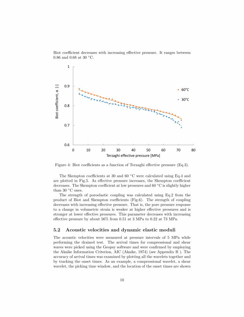
Biot coefficient decreases with increasing effective pressure. It ranges between0.86 and 0.68 at 30 ◦C.

0 10 20 30 40 50 60 70 80

0.6

0.7

0.8

0.9

1

Terzaghi effective pressure [MPa]

Bio

t co

effi

cien

t, α

[-]

60°C

30°C

Figure 4: Biot coefficients as a function of Terzaghi effective pressure (Eq.3).

The Skempton coefficients at 30 and 60 ◦C were calculated using Eq.4 andare plotted in Fig.5. As effective pressure increases, the Skempton coefficientdecreases. The Skempton coefficient at low pressures and 60 ◦C is slightly higherthan 30 ◦C ones.

The strength of poroelastic coupling was calculated using Eq.2 from theproduct of Biot and Skempton coefficients (Fig.6). The strength of couplingdecreases with increasing effective pressure. That is, the pore pressure responseto a change in volumetric strain is weaker at higher effective pressures and isstronger at lower effective pressures. This parameter decreases with increasingeffective pressure by about 56% from 0.51 at 3 MPa to 0.22 at 73 MPa.

5.2 Acoustic velocities and dynamic elastic moduli

The acoustic velocities were measured at pressure intervals of 5 MPa whileperforming the drained test. The arrival times for compressional and shearwaves were picked using the Geopsy software and were confirmed by employingthe Akaike Information Criterion, AIC (Akaike, 1974) (see Appendix B ). Theaccuracy of arrival times was examined by plotting all the wavelets together andby tracking the onset times. As an example, a compressional wavelet, a shearwavelet, the picking time window, and the location of the onset times are shown

10

0 10 20 30 40 50 60 70 80

0.2

0.3

0.4

0.5

0.6

0.7

Terzaghi effective pressure [MPa]

Skem

pto

n c

oef

fici

ent,

B [

-]

60°C

30°C

Figure 5: Skempton coefficients as a function of Terzaghi effective pressure(Eq.4).

in Fig.7.Figures 8 and 9 present the compressional and shear wave velocities as a

function of effective pressure at 30 and 60 ◦C, respectively. The P- and S-wave velocities approached a maximum value of about 5.12 and 2.68 km/s withincreasing pressure at 30 ◦C, respectively. The P-wave velocity increased withincreasing pressure by about 2.5% (from 4.99 to 5.12 km/s) and S-wave velocityincreased by about 2.8% (from 2.60 to 2.68 km/s). At 60 ◦C, the P-wave velocityincreased by about 3.0% (from 4.8 to 4.94 km/s) and S-wave velocity increasedby about 2.73% (from 2.60 to 2.67 km/s).

The velocity ratios for 30 and 60 ◦C are presented in Fig.10. The differencebetween the velocity ratios at 30 and 60 ◦C is higher at low effective pressuresand decreases towards high effective pressures, such that both curves converge.The average velocity ratios at 30 and 60 ◦C are 1.91 and 1.90, respectively.

The dynamic undrained Poisson ratio was calculated using Eq.8 (Fig.11).Poisson’s ratio at 30 ◦C is higher than at 60 ◦C in average. The uncertaintyin calculated Poisson’s ratio can be estimated, using Eq.7 and the method ofpropagation of errors as follows,

∆ν

ν= f(η)

[(∆VPVP

)2

+

(∆VSVS

)2]0.5

(15)

11

0 10 20 30 40 50 60 70 80

0

0.1

0.2

0.3

0.4

0.5

0.6

Terzaghi effective pressure [MPa]

Stre

ngt

h o

f co

up

ling,

aB

[-]

60°C

30°C

Figure 6: Strength of poroelastic coupling, αB, as a function of effective pres-sure.

where

f(η) =2η2

(η2 − 1)(η2 − 2)(16)

A 0.1% error in laboratory measurements of VP and VS yields an error of 0.25%in Poisson’s ratio (0.310± 0.001), whereas a maximum error of 2% in field mea-surements of VP and VS results in a 5% error in Poisson’s ratio calculation(0.31± 0.015). At 30 ◦C, Poisson’s ratio first decreases with increasing effectivepressure and then increases after 60 MPa. At 60 ◦C, Poisson’s ratio is almostconstant at low to moderate effective pressures and increases with increasingeffective pressure after 55 MPa.

5.3 Relating static and dynamic elastic moduli

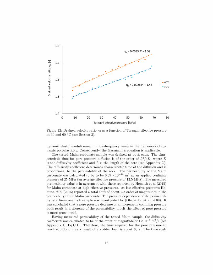
The undrained dynamic elastic bulk moduli were calculated, having obtainedthe ultrasonic velocity ratios and using Eq.8. The drained velocity ratio wasdetermined by calculating the static poroelastic coupling parameter and themeasured (undrained) velocity ratio (see Fig.12). The rate of change in drainedvelocity ratio with effective pressure at 60 ◦C is slightly higher than at 30 ◦C.

The value of Ku

µ in Eq.12 was obtained as best fit parameter. At 30 ◦C, itwas equal to 3.26, corresponding to an undrained static Poisson’s ratio of 0.28(Eq.9b), and at 60 ◦C it was equal to 2.9, corresponding to an undrained static

12

-1800

-1600

-1400

-1200

-1000

-0.8

-0.6

-0.4

-0.2

0

0.2

0.4

0.6

0.8

10E-6 20E-6 30E-6 40E-6 50E-6 60E-6

AIC

Am

plit

ude

[V

olts]

Time [Sec]

tp

(a) P-wavelet

-2500

-2000

-1500

-1000

-500

-0.4

-0.3

-0.2

-0.1

0

0.1

0.2

0.3

0.4

40E-6 45E-6 50E-6 55E-6 60E-6 65E-6 70E-6

AIC

Am

plit

ud

e [

Vo

lts]

Time [Sec]

ts

(b) S-wavelet

Figure 7: Detecting the onset of arrival times (tp and ts) was performed byemploying the Akaike Information Criterion (AIC) for both P- and S-wavelets.The minimum value of the AIC function corresponds to the first motion of thewaves.

13

4900

4950

5000

5050

5100

5150

0 10 20 30 40 50 60 70 80

Co

mp

ress

ion

al w

ave

velo

city

, VP

[m/s

]

Terzaghi effective pressure [MPa]

30°C

60°C

Figure 8: Compressional wave velocity VP as a function of Terzaghi effectivepressure at 30 and 60 ◦C.

Poisson’s ratio of 0.24. The drained bulk moduli were derived by employingEq.8 and by substituting the drained velocity ratios that matched properly themeasured static drained bulk moduli (Figs. 13 and 14).

6 Discussion

Previous studies tried to correlate the static and dynamic moduli either bycorrecting for stress-strain measurements, e.g. Fjaer (1999) and Holt et al (2012)or by defining compressional and shear wave velocities in terms of effectivemoduli and randomly distributed inclusions (Le Ravalec and Gueguen, 1996).Messop (2012) ascribed the difference between static and dynamic moduli to thetime scale of pressure diffusion processes and the applied boundary conditionsin a poroelastic medium. An effect of applied boundary conditions in quasi-static theory of poroelasticity is reflected here in drained and undrained velocityratios that are related to drained and undrained Poisson ratios, respectively.The introduced correlation approach focuses on the velocity ratio which can bedirectly determined in seismological and geophysical studies (Audet et al, 2009).Albeit, there are some inherited assumptions and limitations.

14

2580

2600

2620

2640

2660

2680

2700

0 10 20 30 40 50 60 70 80

Shea

r w

ave

velo

city

, Vs

[m

/s]

Terzaghi effective pressure [MPa]

30°C

60°C

Figure 9: Shear wave velocity VS as a function of Terzaghi effective pressure at30 and 60 ◦C.

6.1 Assumptions and limitations

The correlation equation (Eq.12) derived from quasi-static Biot theory of poroe-lasticity and Gassmann’s equation applies under the following conditions: a) theporous material is assumed to be linear, isotropic and elastic, b) the porous rockis completely saturated, c) the bulk density is assumed to be constant, d) theporous rock consists of one type of pores such that all pores have the samestiffness, e) the shear moduli at drained and undrained conditions are equal,f) all pores are well connected and the pore pressure is equilibrated within REVg) the induced pore pressures are equilibrated through the pore space at lowand moderate frequencies, and h) the velocity dispersion and attenuation, as aresult of scattering, viscoelastic and solid dissipation, etc. are negligible.

It was assumed that the porous medium is isotropic and Poisson’s ratio isdirectly related to the velocity ratio. In this case, the velocity ratio generallytrends between the velocity ratio of the mineral grains and the values for a sus-pended mixture of fluid and minerals. However, in an anisotropic medium thePoisson ratio and the velocity ratio depend on the orientation of wave propaga-tion, crack density, and crack geometry (Walsh, 1966; Mavko et al, 2003).

15

1.88

1.89

1.9

1.91

1.92

1.93

1.94

0 10 20 30 40 50 60 70 80

Vel

oci

ty r

atio

, [-

]

Terzaghi effective pressure [MPa]

30°C

60°C

Figure 10: Velocity ratio η as a function of Terzaghi effective pressure at 30 and60 ◦C.

6.2 Elastic wave propagation theories

The fundamental equations of elastic wave propagation were derived by assum-ing that dissipation only depends on the relative motion between the fluid andthe solid (Biot, 1956b). Several other dissipation mechanisms can be assumed,such as viscoelastic and solid dissipation (Biot, 1962), and different wave prop-agation theories can be derived for porous and cracked media as reviewed byLe Ravalec and Gueguen (1996) and Sarout (2012). Each characteristic (cut-off) frequency is related to a dissipation mechanism and categorizes the wavepropagation theories into different domains. In addition, each characteristicfrequency determines the transition from a low to a high frequency range, cor-responding to relaxed and unrelaxed dynamic moduli, respectively (Le Ravalecand Gueguen, 1996; Mavko et al, 2003) which should be distinguished fromdrained and undrained moduli.

6.3 Drained and undrained conditions in low frequencyrange

In this experimental study, static and dynamic moduli were simultaneously mea-sured. Therefore, two different types of deformations may occur concurrently;a macroscopic deformation due to applied hydrostatic confining pressure, and amicroscopic deformation due to passage of an ultrasonic stress wave that may

16

0.307

0.308

0.309

0.31

0.311

0.312

0.313

0.314

0 10 20 30 40 50 60 70 80 90

Pois

son

's r

atio

, n [

-]

Terzaghi effective pressure [MPa]

30°C

60°C

Figure 11: Poisson’s ratio ν as a function of Terzaghi effective pressure at 30and 60 ◦C.

induce pore pressure gradients on the scale of individual pores.In quasi-static theory of poroelasticity, the drained and undrained moduli

refer to deformation of the REV and reflect the type of hydraulic boundaryconditions applied to an idealized continuous medium, i.e. the static moduli aremacroscopic effective moduli defined over an REV. The drained and undraineddynamic moduli are characterized by time dependent processes (e.g., the porepressure diffusion and crack closure) within an REV and by hydraulic and me-chanical boundary conditions. Therefore, not only heterogeneities and spatialdistribution of the microscopic properties (e.g., crack aspect ratio and pore ra-dius) are of importance but also the diffusivity coefficient of the rock underconsideration as well as the applied loading rate play an important role (De-tournay and Cheng, 1993; Le Ravalec and Gueguen, 1996). That is, how fast theinduced pore pressure due to the applied stress wave equilibrated with pressuresat the boundaries.

The Biot characteristic frequency separates the quasi-static and dynamicdomains of poroelasticity theory, corresponding to a low and a high frequencyrange, respectively (Le Ravalec and Gueguen, 1996; Sarout, 2012). The Biotcharacteristic frequency of the tested Malm carbonate was calculated using Eq.5to be 13.2 GHz (k=0.69 ×10−18, µf = 8 × 10−4 and φ=0.109). The ultrasonicfrequency in the laboratory (500 KHz) was always less than the Biot charac-teristic frequency. Therefore, the ultrasonic velocity measurements and derived

17

d = 0.0033 P' + 1.52

d = 0.0028 P' + 1.48

1.4

1.5

1.6

1.7

1.8

0 10 20 30 40 50 60 70 80

Dra

ined

vel

oci

ty r

atio

, d

[-]

Terzaghi effective pressure [MPa]

60°C

30°C

Figure 12: Drained velocity ratio ηd as a function of Terzaghi effective pressureat 30 and 60 ◦C (see Section 3).

dynamic elastic moduli remain in low-frequency range in the framework of dy-namic poroelasticity. Consequently, the Gassmann’s equation is applicable.

The tested Malm carbonate sample was drained at both ends. The char-acteristic time for pore pressure diffusion is of the order of L2/4D, where Dis the diffusivity coefficient and L is the length of the core (see Appendix C).The diffusivity coefficient determines characteristic time of the diffusion and isproportional to the permeability of the rock. The permeability of the Malmcarbonate was calculated to be to be 0.69 ×10−18 m2 at an applied confiningpressure of 25 MPa (an average effective pressure of 12.5 MPa). The measuredpermeability value is in agreement with those reported by Homuth et al (2015)for Malm carbonate at high effective pressures. At low effective pressures Ho-muth et al (2015) reported a total shift of about 2-3 order of magnitudes in thepermeabilty of the Malm carbonate. The pressure dependence of the permeabil-ity of a limestone rock sample was investigated by (Ghabezloo et al, 2009). Itwas concluded that a pore pressure decrease or an increase in confining pressureboth result in a decrease of the permeability, albeit the effect of pore pressureis more pronounced.

Having measured permeability of the tested Malm sample, the diffusivitycoefficient was calculated to be of the order of magnitude of 1×10−4 m2/s (seeAppendix C, Eq.C.1). Therefore, the time required for the pore pressure toreach equilibrium as a result of a sudden load is about 60 s. The time scale

18

5

10

15

20

25

30

35

40

45

0 10 20 30 40 50 60 70 80

Bu

lk m

od

ulu

s, K

[G

Pa]

Terzaghi effective pressure [MPa]

Dynamic bulk modulus

Static bulk modulus

Effective bulk modulus

Figure 13: Bulk moduli as a function of Terzaghi effective pressure at 30 ◦C.The effective drained bulk modulus was calculated by substituting the drainedvelocity ratio in Eq.8. The calculated effective and measured static bulk modulimatched well.

19

5

10

15

20

25

30

35

40

45

0 10 20 30 40 50 60 70 80

Bu

lk m

od

ulu

s, K

[G

Pa]

Terzaghi effective pressure [MPa]

Dynamic bulk modulus

Static bulk modulus

Effective bulk modulus

Figure 14: Bulk moduli as a function of Terzaghi effective pressure at 60 ◦C.The effective drained bulk modulus was calculated by substituting the drainedvelocity ratio in the Eq.8. The calculated effective and measured static bulkmoduli matched well.

20

of stress wave propagation is inversely proportional to the frequency and isequal to 2×10−6 s. The time scales of pore pressure diffusion and the stresswave propagation differ by seven orders of the magnitude such that microscopicdeformations can be assumed to be undrained ones. Therefore, the ultrasonicwave propagation, the velocity ratios, and the related dynamic elastic moduliare of undrained nature. Moreover, the applied confining pressure rate 0.09MPa/min is low enough (in comparison to a sudden load, i.e. an infinite rate)such that pore pressure has enough time to be equilibrated with pressures atthe boundaries.

6.4 Poroelastic and dynamic moduli of Malm carbonate

The static and dynamic moduli of the tested Malm carbonate increased withincreasing effective pressure and the same behavior has been observed for othertypes of rock, e.g. sandstone (Fjaer, 1999) and chalk (Alam et al, 2012). Thestress-strain curves showed hysteresis and irreversiblity while loading and un-loading the sample. This indicates that part of the work done on the sample isdissipated. Part of the strains were not recovered immediately after unloading(see Fig.1) which can be assigned to time dependent deformation of the sam-ple (e.g., creep, anelasticty, plasticity, etc.). The principal assumption behindthis analysis is that stress cycling effects has been minimized after applyingpreconditioning procedure (see section 4.2).

The value of the unjacketed bulk modulus 103.9 GPa (see Fig.3) was observedto be higher than those reported for calcite (76.8 GPa) and dolomite (94.9 GPa)minerals (Mavko et al, 2003). Such high values for the unjacketed bulk modulushave been reported previously for a limestone of the same age (da Silva et al,2010). The value of the unjacketed bulk modulus of this late Jurassic rockvaried between 60 and 210 GPa at 25.5 MPa effective pressure. If the mineralcomposition is assumed to be homogeneous, a constant unjacketed bulk modulusequal to the mineral bulk modulus is expected. However, if isolated pores andisolated micro-cracks are present, as expected for carbonate rock, the unjacketedbulk modulus may differ from the mineral bulk modulus and approaches a highervalue. Moreover, the composition of the tested Malm carbonate shows existenceof different oxides with bulk moduli higher than 150 GPa (see Table 1) thatinfluences the unjacketed stiffness of the porous rock.

Dimensionless poroelastic coefficients, such as the Biot coefficient, the Skemp-ton coefficient and the strength of poroelastic coupling, decreased with increas-ing effective pressure (see Figs. 4, 5 and 6). That is, the degree of coupling be-tween deformation and pore pressure decreases with increasing effective pressureand pore pressure less effectively counteracts the applied confining pressure re-sulting in lateral deformation of grains into the pore space and to altering poros-ity. Porosity variations and changes in micro-structure provide a link betweenporoelastic and dynamic moduli. Since values of pore stiffness Kφ are rather dif-ficult to be directly measured, the common assumption is that Kφ = Ks (Hartand Wang, 1995). In the current study, an indirect method (Eq. 3) was usedto calculate the Biot coefficient using the static elastic moduli. An alternative

21

approach for determining the poroelastic coupling parameter is to measure theBiot and Skempton coefficients directly, without measuring static elastic mod-uli. That is, the fluid mass content can be monitored to obtain Biot’s coefficient,and the Skempton coefficient can be measured as the ratio of the induced porepressure to the change in applied confining pressure for undrained conditions(Hassanzadegan et al, 2012; Blocher et al, 2014). This has the advantages thatno stress-strain measurements are required and the effective velocity ratio canbe related directly to the poroelastic coupling parameter.

The poroelastic coupling parameter served to accommodate for the nonlin-earity of the dynamic bulk modulus and to include the changes in Poisson’sratio. At low effective pressures, the value of the poroelastic coupling param-eter is high, low aspect ratio pores are open, and Poisson’s ratio is less thanits intrinsic value, i.e. Poisson’s ratio of the rock without cracks (Walsh, 1965).At high effective pressures, the value of the poroelastic coupling parameter de-creases, low aspect ratio pores are closed, and Poisson’s ratio increases withincreasing effective pressure (Walsh, 1965). That is, at high pressures not onlythe low aspect ratio pores are closed but also the grains deform into the porespace due to Poisson’s effect, i.e. compression at grain contacts causes the grainsto become shorter in the direction of the compressive load and wider laterallythereby lowering the effective porosity of the rock. Consequently, acoustic ve-locity increases.

The acoustic velocities were in the range of those reported for Cobourge lime-stone (Nasseri et al, 2013) and were increasing with increasing effective pressure(see Figs.8 and 9). Both VP and VS decreased with increasing temperature from30 to 60 ◦C. While heat treatment, the thermally induced microcracks, and in-creasing crack porosity may lower the acoustic velocities, which has also beenobserved for Bourgogne limestone (Lion et al, 2005) and Flechtinger sandstone(Hassanzadegan et al, 2013).

Since the ultrasonic acoustic velocity ratios are of undrained nature, the de-rived Poisson ratios are also of undrained nature. It appears that this correlation(Eq.12) provides the correct nonlinear link between drained and undrained ve-locity ratios via the strength of poroelastic coupling parameter αB.

Two terms are associated with any discussion of error analysis: accuracyand precision. While the accuracy is a measure of the closeness to the truevalue, the precision refers to reproducibility of the measurements. The errorcalculations presented here refer to the accuracy of the results rather than theirprecision. Thus, this study becomes a starting point for further investigationsat in-situ conditions, for a wide range of frequencies and confining pressures,and including different rock types.

6.5 Implications

6.5.1 Earthquakes and induced seismicity

At the time of an earthquake the static stress change can be considered negligible(Brenguier et al, 2014). However, when seismic energy is released, part of the

22

energy propagates through the crust as seismic body waves resulting in dynamicstress changes, i.e. as transient stress perturbations (Brenguier et al, 2014).Due to the short time scale of an earthquake in comparison to the rate of fluidflow, undrained conditions are favored in the fluid saturated zones and a highervelocity ratio in comparison to drained conditions is expected. There are someobservations and evidence that confirm this hypothesis. For example, passive-source seismic imaging suggested the existence of a zone of high velocity andPoisson ratios down-dip of a subduction ridge which was attributed to high porefluid pressures and low effective pressures (Brenguier et al, 2014). Moreover,Segall (1989) has shown that poroelastic contraction of a zone from which fluidare produced can destabilize faults and induce seismicity in areas where thefluid mass content does not change (i.e. in undrained zones).

Providing the suggested correlation, it would be possible to characterizeundrained zones in terms of poroelastic moduli by comparing seismic imagesbefore and after induced seismicity or earthquakes.

6.5.2 Mechanical reservoir characterization and monitoring

The presented correlation not only can be used for geomechanical reservoir char-acterization but also it is important for underground reservoir management andthe recognition of the overpressured and underpressured zones within geother-mal and hydrocarbon reservoirs before and after exploitation. First, the poroe-lastic moduli in concert with acoustic velocities of a rock sample, representativefor the target formation, have to be measured in the laboratory. Then, thederived correlation between acoustic velocity ratios and the poroelastic moduliserves to characterize the reservoir formation, having obtained the field measure-ments of acoustic velocities. In other words, by comparing initial and modifiedvelocity ratios, the in situ effective pressure and the corresponding poroelasticmoduli can be derived.

7 Conclusions

In this study static drained bulk moduli of Malm carbonate were correlated tothe dynamic elastic bulk moduli. A novel correlation approach was presentedbased on Biot theory of poroleasticity and wave propagation. The strength ofporoelastic coupling parameter, i.e. the product of Biot and Skempton coeffi-cients, was the central element of this coupling approach. A drained velocityratio was introduced and was linked to the drained Poisson ratio. The Biotand Skempton coefficients, as well as their products, i.e. the strength of poroe-lastic coupling, were pressure dependent and were decreasing with increasingpressure. The value of the strength of poroelastic coupling parameter decreasedwith increasing effective pressure by about 56% from 0.51 at 3 MPa to 0.22 at73 MPa. In contrast, the P- and S-wave velocities changed by a maximum of3% in this pressure range. The P- and S-wave velocities approach a maximumvalue of about 5.12 and 2.68 km/s, respectively, with increasing pressure at 30

23

◦C. The average velocity ratios at 30 and 60 ◦C were 1.91 and 1.90, receptively.The calculated drained bulk moduli using the effective velocity ratios matchedthe measured static drained bulk moduli well.

The proposed correlation approach not only is important in detecting andcharacterizing low and high effective pressure zones within subduction zonesbut also is important in underground reservoir management for recognizing andcharacterizing overpressured and underpressured zones within geothermal andhydrocarbon reservoirs, e.g., by comparing velocity ratios before and after in-jection or production.

8 Acknowledgments

The authors would like to thank Liane Liebeskind for assistance with the lab-oratory experiments and TU Bergakademie Freiberg for providing XRD data.Furthermore, the authors would like to thank the reviewers for their construc-tive comments. This work has been performed in the framework of the Allgaugeothermal project and was funded by the Federal Ministry for the Environment,Nature Conservation, Building and Nuclear Safety, Germany (Grant 0325267B).

Nomenclature

Latin Letters

a fitting parameterB Skempton coefficient [-]b fitting parameterE Young’s modulus PaKd drained bulk modulus PaKφ pore stiffness PaKu undrained bulk modulus PaKf pore fluid bulk modulus PaKs solid grain bulk modulus PaKdyu dynamic undrained bulk modulus Pam fluid mass content kgm0 reference fluid mass content kgP confining pressure PaP ′ Terzaghi effective pressure PaPp pore pressure PaVp

VSvelocity ratio [-]

V 0b reference bulk volume m3

VP compressional wave velocity m/sVS shear wave velocity m/sWa suspended weight of the sample kgWd dry weight of the sample kg

24

Ws saturated weight of the sample kg

Greek Letters

α Biot coefficient [-]αB strength of poroelastic coupling [-]ρb bulk density kg/m3

η velocity ratio [-]ηd drained velocity ratio [-]ηu undrained velocity ratio [-]εb bulk strain [-]ν Poisson’s ratio [-]νd drained Poisson’s ratio [-]φ porosity [-]φi initial porosity [-]ρ0 reference fluid density kg/m3

σkk first stress invariant Paµ shear modulus Paµd drained shear modulus Paµu undrained shear modulus Pa

9 Appendices

A Gassmann equation

Gassmann’s equation relates the drained to the undrained bulk moduli. Gassmann’sequations can be written in terms of the strength of the poroelastic couplingαB (Berryman, 1999):

Ku =Kd

1 − αB(A.1)

µd = µu (A.2)

This relation (Eq.A.1) shows how the stiffness of a loaded rock is related tothe strength of the poroelastic coupling. In principle, the drained and undrainedshear moduli, i.e. µd and µu, are identical (Berryman, 1999). At low frequen-cies, the Gassmann equation relates the drained and undrained elastic moduli(Le Ravalec and Gueguen, 1996).

B Picking the arrival-times of ultrasonic waves

A review of time-picking techniques is given by Sarout et al (2009). The AkaikeInformation Criterion (AIC) was used for picking arrival-times of ultrasonicwaves. The AIC picker is a statistical function for which the global minimum

25

defines the onset time of the signal as described by Akaike (1974), Akazawa(2004) and Kurz et al (2005).

AIC(J) = J. log(var(R(1, J))) + (N − J − 1). log(var(R(1 + J,N))) (B.1)

This formulation applies two sliding ranges (windows) to the signal, where Jis a counter range through the signal and N is the total number of data samples.log and var denote the logarithm and variance functions and R(a, b) determinesthe interval range of the recorded voltage.

C Transient poroelasticity

The coupling of fluid mass diffusion with volumetric deformation results in acoupled pore pressure diffusion, i.e. the pore pressure diffusion is coupled withthe rate of change of the volumetric strain. The diffusivity coefficient D can bewritten in terms of drained and undrained elastic moduli, the mobility ratio k

µf,

and poroelastic coefficients to be (Gueguen and Bouteca, 2004),

D =BKu

α

k

µf

(K + 4µ3 )

(Ku + 4µ3 )

(C.1)

References

Akaike H (1974) Markovian representation of stochastic processes and its appli-cation to the analysis of autoregressive moving average processes. Annals ofthe Institute of Statistical Mathematics 26(1):363–387

Akazawa T (2004) A technique for automatic detection of onset time of pands-phases in strong motion records, 13th World conference on earthquake en-gineering vancouver, b.c., canada. In: 13th World Conference on EarthquakeEngineering, pp 1–9

Alam MM, Fabricius IL, Christensen HF (2012) Static and dynamic effectivestress coefficient of chalk. Geophysics 77(2):L1–LL11

Audet P, Bostock MG, Christensen NI, Peacock1 SM (2009) Seismic evidence foroverpressured subducted oceanic crust and megathrust fault sealing. Nature457:76–78

Berryman JG (1999) Origin of Gassmann’s equations. Geophysics 64(5):1627–1629

Biot MA (1941) General theory of three-dimensional consolidation. Journal ofApplied Physics 12(2):155–164

Biot MA (1956a) Theory of propagation of elastic waves in a fluid-saturatedporous solid. i. low-frequency range. Journal of the Acoustical Society ofAmerica 28(2):168–178

26

Biot MA (1956b) Theory of Propagation of Elastic Waves in a Fluid-SaturatedPorous Solid. II. higher-Frequency Range. The Journal of the Acoustical So-ciety of America 28:179–191

Biot MA (1962) Generalized theory of acoustic propagation in porous dissipativemedia. The Journal of the Acoustical Society of America 34(9A):1254–1264

Blocher G, Reinsch T, Hassanzadegan A, Milsch H, Zimmermann G (2014)Direct and indirect laboratory measurements of poroelastic properties of twoconsolidated sandstones. International Journal of Rock Mechanics and MiningSciences 67:191 – 201

Brenguier F, Campillo M, Takeda T, Aoki Y, Shapiro NM, Briand X, EmotoK, Miyake H (2014) Mapping pressurized volcanic fluids from induced crustalseismic velocity drops. Science 345(6192):80–82

Cacace M, Blocher G, Watanabe N, Moeck I, Borsing N, Magdalena-Scheck-Wenderoth, Kolditz O, Huenges E (2013) Modelling of fractured carbonatereservoirs: outline of a novel technique via a case study from the molassebasin, southern bavaria, germany. Environmental Earth Sciences 70(8):3585–3602

Carmichael R (1984) Handbook of physical properties of rocks, Handbook ofPhysical Properties of Rocks, vol v. 3. Taylor and Francis

Carroll M (1980) Mechanical response of fluid suturated porous materials. In:Theoretical and Applied Mechanics, Proc. 15th Int. Congress of Theoreti-cal and Applied Mechanics, Toronto, August 1723, F. P. J. Rimrott and B.Tabarrok, eds., North-Holland, Amsterdam, pp 251–262

Castagna JP, Batzle ML, Eastwood RL (1985) Relationships betweencompressional-wave and shear-wave velocities in clastic silicate rocks. Geo-physics 50(4):571–581

Detournay E, Cheng AHD (1993) Fundamentals of poroelasticity. In Compre-hensive Rock Engineering: Principles, Practice and Projects, vol 2, PergamonPress, chap 5, pp 113 –169

Eissa E, Kazi A (1988) Relation between static and dynamic young’s moduliof rocks. International Journal of Rock Mechanics and Mining Sciences andGeomechanics Abstracts 25(6):479 – 482

Fjaer E (1999) Static and dynamic moduli of weak sandstones. In: Rock Me-chanics for Industry Amadei, B., Kranz, RL, Scott, GA, Smeallie, Balkema,pp 675–681

Gassmann (1951) Uber die Elastizitat poroser Medien. Vierteljahrsschrift derNaturforschenden Gesellschaft 96:1–23

27

Ghabezloo S, Sulem J, Gudon S, Martineau F (2009) Effective stress law forthe permeability of a limestone. International Journal of Rock Mechanics andMining Sciences 46(2):297 – 306

Gueguen Y, Bouteca M (2004) Mechanics of Fluid Saturated Rocks. ElsevierAcademic Press

Hart DJ, Wang HF (1995) Laboratory measurements of a complete set of poroe-lastic moduli for berea sandstone and indiana limestone. Journal of Geophys-ical Research: Solid Earth 100(B9):17,741–17,751

Hassanzadegan A, Blocher G, Zimmermann G, Milsch H (2012) Thermoporoe-lastic properties of flechtinger sandstone. International Journal of Rock Me-chanics and Mining Sciences 49(0):94 –104

Hassanzadegan A, Blocher G, Milsch H, Urpi L, Zimmermann G (2013) Theeffects of temperature and pressure on the porosity evolution of Flechtingersandstone. Rock Mechanics and Rock Engineering 47(2):421–434

Heerden W (1987) General relations between static and dynamic moduli ofrocks. International Journal of Rock Mechanics and Mining Sciences and Ge-omechanics Abstracts 24(6):381 – 385

Hofmann H, Blocher G, Borsing N, Maronde N, Pastrik N, Zimmermann G(2014) Potential for enhanced geothermal systems in low permeability lime-stones stimulation strategies for the western Malm karst (Bavaria). Geother-mics 51:351 – 367

Holt RM, Nes OM, F SJ, Fjaer E (2012) Static vs. dynamic behavior ofshale. In: American Rock Mechanics Association, 46th U.S. Rock Mechan-ics/Geomechanics Symposium, 24-27 June, Chicago, IL, USA

Homuth S, Gotz AE, Sass I (2015) Reservoir characterization of the upperjurassic geothermal target formations (molasse basin, germany): role of ther-mofacies as exploration tool. Geothermal Energy Science 3(1):41–49, DOI10.5194/gtes-3-41-2015

King MS (1969) Static and dynamic elastic moduli of rocks under pressure. In:The 11th U.S. Symposium on Rock Mechanics (USRMS), June 16 - 19, 1969, Berkeley, CA, pp 329–351

Kurz JH, Grosse CU, Reinhardt HW (2005) Strategies for reliable automaticonset time picking of acoustic emissions and of ultrasound signals in concrete.Ultrasonics 43(7):538 – 546

Le Ravalec M, Gueguen Y (1996) High- and low-frequency elastic moduli fora saturated porous/cracked rock-differential self-consistent and poroelastictheories. Geophysics 61(4):1080–1094

28

Lion M, Skoczylas F, Ledesert B (2005) Effects of heating on the hydraulic andporoelastic properties of bourgogne limestone. International Journal of RockMechanics and Mining Sciences 42(4):508–520

Mavko G, Mukerji T, Dvorkin J (2003) The Rock Physics Handbook: Tools forSeismic Analysis of Porous Media. Cambridge University Press

Messop A (2012) When to use static or dynamic moduli in geomechanical mod-els. In: 46th US Rock Mechanics / Geomechanics Symposium , 24-27 June,held in Chicago, IL, USA

Nasseri M, Goodfellow S, Wanne T, Young R (2013) Thermo-hydro-mechanicalproperties of cobourg limestone. International Journal of Rock Mechanics andSciences, Mining 61:212–222

Nur A, Byerlee JD (1971) An effective stress law for elastic deformation of rockwith fluids. Journal of Geophysical Research 76:6414–6419

Sarout J (2012) Impact of pore space topology on permeability, cut-off frequen-cies and validity of wave propagation theories. Geophysical Journal Interna-tional 189(1):481–492

Sarout J, Ferjani M, Guguen Y (2009) A semi-automatic processing techniquefor elastic-wave laboratory data. Ultrasonics 49(45):452 – 458

Sayers CM, Schutjens PMTM (2007) An introduction to reservoir geomechanics.The Leading Edge 26(5):597–601

Segall P (1989) Earthquakes triggered by fluid extraction. Geology 17(10):942–946

da Silva MR, Schroeder C, Verbrugge JC (2010) Poroelastic behaviour of awater-saturated limestone. International Journal of Rock Mechanics and Min-ing Sciences 47(5):797–807

Simmons G, Brace WF (1965) Comparison of static and dynamic measurementsof compressibility of rocks. Journal Of Geophysical Research 70:5649–5656

Walsh JB (1965) The effect of cracks in rocks on poisson’s ratio. Journal ofGeophysical Research 70(20):5249–5257

Walsh JB (1966) Seismic wave attenuation in rock due to friction. Journal ofGeophysical Research 71(10):2591–2599

Wang Z (2000) Dynamic versus static elastic properties of reservoir rocks. In:Seismic and Acoustic Velocities in Reservoir Rocks: Recent developments,Seismic and Acoustic Velocities in Reservoir Rocks, Society of ExplorationGeophysicists, pp 531–539

Wathele M (2004) Geopsy project. In: Grenoble, France, URL http://www.

geopsy.org

29

Yale DP, Jamieson WH (1994) Static and dynamic mechanical properties ofcarbonates. In: Rock Mechanics, Balkema, Rotterdam

Zimmerman R (2000) Coupling in poroelasticity and thermoelasticity. Interna-tional Journal of Rock Mechanics and Mining Sciences 37(1-2):79 – 87

30