HASP Program Flight Readiness Review Document for …laspace.lsu.edu/pacer/Experiment/2010/... ·...
105
Team EQUIS i FRR v1.0 HASP Program Flight Readiness Review Document for the Attitude Determination System (ADS) Experiment by Experiments with Quality United In Science (EQUIS) Prepared by: Team Leader: Dr. H. B. Vo/E.G.Delgado 7/23/2010 Team Member: A. M. Espinal Mena 7/23/2010 Team Member: F. O. Rivera Vélez 7/23/2010 Team Member: E.M. Portilla Matías 7/23/2010 Team Member: J. I. Espinosa Acevedo 7/23/2010 Submitted: Reviewed: Revised: Approved: Dr. Greg Guzik 7/23/2010 Institution Signoff Date HASP Signoff Date
Transcript of HASP Program Flight Readiness Review Document for …laspace.lsu.edu/pacer/Experiment/2010/... ·...

Team EQUIS i FRR v1.0
HASP Program
Flight Readiness Review Document for the Attitude Determination System (ADS)
Experiment by Experiments with Quality United In Science
(EQUIS)
Prepared by: Team Leader: Dr. H. B. Vo/E.G.Delgado 7/23/2010
Team Member: A. M. Espinal Mena 7/23/2010
Team Member: F. O. Rivera Vélez 7/23/2010
Team Member: E.M. Portilla Matías 7/23/2010
Team Member: J. I. Espinosa Acevedo 7/23/2010
Submitted:
Reviewed:
Revised:
Approved: Dr. Greg Guzik 7/23/2010
Institution Signoff Date
HASP Signoff Date

Team EQUIS ii FRR v1.0
Change Information Page
Title: FRR Document for ADS Experiment Date: 07/23/2010
List of Effected Pages
Page Number Issue Date

Team EQUIS iii FRR v1.0
Status of TBDs
TBD
Number
Section Description Date
Created
Date
Resolved

Team EQUIS iv FRR v1.0
Table of Contents Experiment by .............................................................................................................................. i
Change Information Page ........................................................................................................... ii
Status of TBDs ...........................................................................................................................iii
Table of Contents ....................................................................................................................... iv
List of Figures ............................................................................................................................ vi
List of Tables ...........................................................................................................................viii
1.0 Document Purpose ................................................................................................................ 9
1.1 Document Scope ............................................................................................................... 9
1.2 Change Control and Update Procedures ........................................................................... 9
2.0 Reference Documents ........................................................................................................... 9
3.0 Goals, Objectives, Requirements ........................................................................................ 11
3.1 Mission Goal ................................................................................................................... 11
3.2 Objectives ....................................................................................................................... 11
3.3 Science Background and Requirements.......................................................................... 12
3.4 Technical Background and Requirements ...................................................................... 25
4.0 Payload Design ................................................................................................................... 30
4.1 Principle of Operation ..................................................................................................... 30
4.2 System Design ................................................................................................................ 30
4.3 Electrical Design ............................................................................................................. 37
4.4 Software Design .............................................................................................................. 44
4.5 Thermal Design ............................................................................................................... 50
4.6 Mechanical Design.......................................................................................................... 52
5.0 Payload Development Plan ................................................................................................. 58
6.0 Payload Construction Plan .................................................................................................. 59
6.1 Hardware Fabrication and Testing .................................................................................. 59
6.2 Integration Plan ............................................................................................................... 59
6.3 Software Implementation and Verification ..................................................................... 60
6.4 Flight Certification Testing ............................................................................................. 61
7.0 Mission Operations ............................................................................................................. 63
7.1 Pre-Launch Requirements and Operations ..................................................................... 63
7.2 Flight Requirements, Operations and Recovery ............................................................. 70
7.3 Data Acquisition and Analysis Plan ............................................................................... 70
8.0 Project Management ........................................................................................................... 71
Team EQUIS v FRR v1.0
8.1 Organization and Responsibilities .................................................................................. 71
8.2 Configuration Management Plan .................................................................................... 71
8.3 Interface Control ............................................................................................................. 71
9.0 Master Schedule .................................................................................................................. 72
9.1 Work Breakdown Structure (WBS) ................................................................................ 72
9.2 Staffing Plan.................................................................................................................... 72
9.3 Timeline and Milestones ................................................................................................. 73
10.0 Master Budget ................................................................................................................... 73
10.1 Expenditure Plan ........................................................................................................... 73
11.0 Risk Management and Contingency ................................................................................. 74
12.0 Glossary ............................................................................................................................ 76
Appendix ................................................................................................................................... 77
Appendix A ........................................................................................................................... 77
Appendix B ........................................................................................................................... 80
Sensors Subsystem Schematic and PCB design ............................................................... 80
Appendix C ........................................................................................................................... 82
RTC (DS1306) pseudo code ............................................................................................. 82
Magnetometer (MicroMag3) pseudo code ........................................................................ 83
Accelerometer (SCA3000-D01) pseudo code ................................................................. 85
SD card pseudo code ......................................................................................................... 86
Pre-flight software ............................................................................................................ 87
During flight software ....................................................................................................... 91
Appendix D ......................................................................................................................... 103
Team EQUIS vi FRR v1.0
List of Figures
Figure 1: Three axis center mass reference frame and their rotational change definition ........ 13 Figure 2: Accelerometer average values ................................................................................... 14 Figure 3: Accelerometer maximum values ............................................................................... 14 Figure 4: Gyroscope basic structure and operation ................................................................... 15
Figure 5: Earth's Magnetic Field ............................................................................................... 16 Figure 6: Magnitude of the earth’s magnetic field .................................................................... 17 Figure 7: Parameters of the magnetic field ............................................................................... 17 Figure 8: Vector's example of the magnetic field ..................................................................... 18 Figure 9: Vector’s example of the magnetic field .................................................................... 18
Figure 10: Angles of interest ..................................................................................................... 19 Figure 11: HASP 2006 flight profile ........................................................................................ 20
Figure 12: Payload trajectory dynamics ................................................................................... 20 Figure 13: Angle of translation determination .......................................................................... 21 Figure 14: Angle of translation determination .......................................................................... 21 Figure 15 Beamwidth shade diameter determination ............................................................... 21
Figure 16: Determining position accuracy ................................................................................ 22 Figure 17: Determining position accuracy with orbit decay ..................................................... 22 Figure 18: Plot of typical orbit decay ....................................................................................... 23
Figure 19: Temperature variation during flight ........................................................................ 24 Figure 20: Accelerometers basic principal of operation ........................................................... 25
Figure 21: Gyroscopes basic principal of operation ................................................................. 26 Figure 22: Simplified representation of magnetometer basic operations ................................. 27 Figure 23: The DS18B20 Digital temperature sensor............................................................... 28
Figure 24: DS18B20 Digital Temperature Sensor Diagram (From the DS18B20 datasheet) .. 28
Figure 25: Determination of sampling rate by maximum angular velocity .............................. 29 Figure 26: ADS System Design ................................................................................................ 30 Figure 27: Arduino Pro 328 3.3V/8MHz schematic ................................................................. 31
Figure 28: Three Axis Accelerometer schematic ...................................................................... 31 Figure 29: Three Axis Magnetometer schematic ...................................................................... 32
Figure 30: Three Axis Gyroscope schematic ............................................................................ 32 Figure 31: Digital Temperature Sensor schematic .................................................................... 32 Figure 32: MicroSD board schematic ....................................................................................... 33 Figure 33: Real-Time Clock schematic .................................................................................... 33
Figure 34: 9V DC to DC Converter schematic ......................................................................... 33 Figure 35: 3.3V Voltage Regulator schematic .......................................................................... 34 Figure 36: 5V Voltage Regulator schematic ............................................................................. 34
Figure 37: Electrical Design Subsystems ................................................................................. 37 Figure 38: Electrical Subsystem ............................................................................................... 37 Figure 39: Accelerometer Sensor.............................................................................................. 38 Figure 40: SCA3000 Three axis accelerometer pins ................................................................ 38
Figure 41: Gyroscope Sensor .................................................................................................... 39 Figure 42: Three Axis Magnetometer ....................................................................................... 39 Figure 43: Digital Temperature Sensor ..................................................................................... 39
Figure 44: Real Time Clock ...................................................................................................... 40

Team EQUIS vii FRR v1.0
Figure 45: ADS PCB Design .................................................................................................... 41
Figure 46: Power System Diagram ........................................................................................... 42 Figure 47: Power Budget Analysis ........................................................................................... 44 Figure 48: Flight software control flow chart ........................................................................... 49
Figure 49:Payload”s Top Cover ................................................................................................ 53 Figure 50: Internal View of the External Structure .................................................................. 54 Figure 51: External Structure Drawing ..................................................................................... 54 Figure 52: Finite Element Analysis View 1 .............................................................................. 55 Figure 53 Finite Element Analysis View 2 ............................................................................... 55
Figure 54: Detail drawings of payload...................................................................................... 56 Figure 55: Top view payload structure ..................................................................................... 56 Figure 56: View of punctures on structures .............................................................................. 57 Figure 57: Internal Structure Drawing ...................................................................................... 57
Figure 58: EDAC pin layout ..................................................................................................... 60 Figure 59 Psi Vacuum chamber ................................................................................................ 61
Figure 60 Chamber where temperature test was taken ............................................................. 62 Figure 61: Shock Test ............................................................................................................... 62
Figure 62 Helmholtz coils ......................................................................................................... 64 Figure 63: Helmholtz coil (X) vs MM3 (Y) ............................................................................. 66 Figure 64: Linear Fit ................................................................................................................. 69
Figure 65: WBS- Work Breakdown Schedule .......................................................................... 72 Figure 66: Risk Management Cycle ......................................................................................... 75
Figure 68: Heat Loss Analysis .................................................................................................. 77 Figure 69: External Convention ................................................................................................ 79
Team EQUIS viii FRR v1.0
List of Tables
Table 1: Traceability Matrix ..................................................................................................... 36 Table 2: Pins for the Pro 328 .................................................................................................... 40 Table 3: Power Requirements ................................................................................................... 43 Table 4: Bytes Description........................................................................................................ 45
Table 5: SPCR bit specification ................................................................................................ 46 Table 6: RTC registers and address map .................................................................................. 46 Table 7: Axis Select .................................................................................................................. 47 Table 8: SCA3000 registers ...................................................................................................... 47 Table 9: Electronic temperature limits ...................................................................................... 50
Table 10: Effects of the surface treatment in the emisivity ...................................................... 52 Table 11: Alloy Selection ......................................................................................................... 52
Table 12 Polyester Properties ................................................................................................... 57 Table 13: Mass Budget ............................................................................................................. 58 Table 14: EDAC 516 pins function and color code .................................................................. 60 Table 15 Example of raw data from the MM3 ......................................................................... 65
Table 16: Calibration values ..................................................................................................... 65 Table 17: Equations to correct offset ........................................................................................ 65 Table 18: Quadrant determination ........................................................................................... 66
Table 19: DS18B20 versus HOBO temperature measures ....................................................... 68 Table 20: Materials Acquirement & Costs ............................................................................... 74
Table 21: Risk Management & Contingency............................................................................ 75

Team EQUIS 9 FRR v1.0
1.0 Document Purpose
This document describes the final designs for the Attitude Determination System (A.D.S.)
experiment by Team EQUIS for the HASP Program. It fulfills part of the HASP Project
requirements for the Flight Readiness Review (FRR) to be held July 23, 2010.
1.1 Document Scope
This FRR document specifies the scientific purpose and requirements for the A.D.S.
experiment and provides a guideline for the development, operation, and cost of this payload
under the HASP Project. The document includes details of the payload design, fabrication,
integration, testing, flight operation, and data analysis. In addition, project management,
timelines, work breakdown, expenditures, and risk management is discussed. Finally, the
designs and plans presented here are preliminary.
1.2 Change Control and Update Procedures
Changes to this FRR document shall only be made after approval by designated
representatives from Team EQUIS and the HASP Institution Representative. Document
modification requests should be sent to Team members, the HASP Institution Representative
and the HASP Project.
2.0 Reference Documents
The following websites are references for relevant scientific information as well as sources of
electronic components, their specifications, part numbers, products availability, and prices.
Bibliography:
[1] (USRA), R. N. (2002, November 25). Astronomy Picture of the Day. Retrieved May
24, 2010, from Astronomy Picture of the Day Web site:
http://www.astronet.ru/db/xware/msg/1181025
[2] Analog Devices Corporate Headquarters. (2008, September). Analog Devices.
Retrieved May 24, 2010, from Analog Devices Web site: http://www.analog.com
[3] Arduino Pro. (2010). Retrieved March 28, 2010, from Arduino:Blog:
http://arduino.cc/en/Main/ArduinoBoardPro, March 28, 2010
[4] Biology Blog. (n.d.). Retrieved May 24, 2010, from Biology Blog Web Site:
http://www.biology-blog.com/blogs/permalinks/7-2007/chickens-and-earths-magnetic-
field.html
[5] Field Code. (2008). Retrieved February 3, 2010, from Whatis?com Web site:
http://whatis.techtarget.com/definition/0,,sid9_gci213703,00.html
[6] kowoma.de. (2009, April 19). Retrieved May 24, 2010, from kowoma.de Web site:
http://www.kowoma.de/en/gps/additional/atmosphere.htm

Team EQUIS 10 FRR v1.0
[7] Metrolab Instruments. (2006, October). Metrolab Instruments. Retrieved May 24,
2010, from MetroLab Manufactures of MRI systems:
http://www.metrolab.com/index.php?id=10
[8] Mystery Class. (2008). Retrieved May 24, 2010, from Mystery Class Journy North
Web site: http://www.learner.org/jnorth/tm/mclass/Glossary.html
[9] Ritter, M. E. (2009). The Physical Environment an Introduction to Physical
Geography. Retrieved May 24, 2010, from
http://www.uwsp.edu/geo/faculty/ritter/geog101/textbook/energy/earth_sun_relations_
seasons.html
[10] Sparkfun. (2003). Retrieved May 24, 2010, from Sparkfun website:
http://www.sparkfun.com
[11] Wikipedia (DC-to-DC Converters). (2010). Retrieved April 4, 2010, from Wikipedia
Web site: http://en.wikipedia.org/wiki/DC-to-DC_converter
[12]Anderson, B. J., editor, and R. E. Smith, compiler, Natural Orbital Environment
Guidelines for Use in Aerospace Vehicle Development, NASA TM 4527, chapters 6
and 9, June 1994.
[13] T Williams & P Collins, 1997, "Orbital Considerations in Kankoh-Maru Rendezvous
Operations", Proceedings of 7th ISCOPS, AAS Vol 96, pp 693-707.
Team EQUIS 11 FRR v1.0
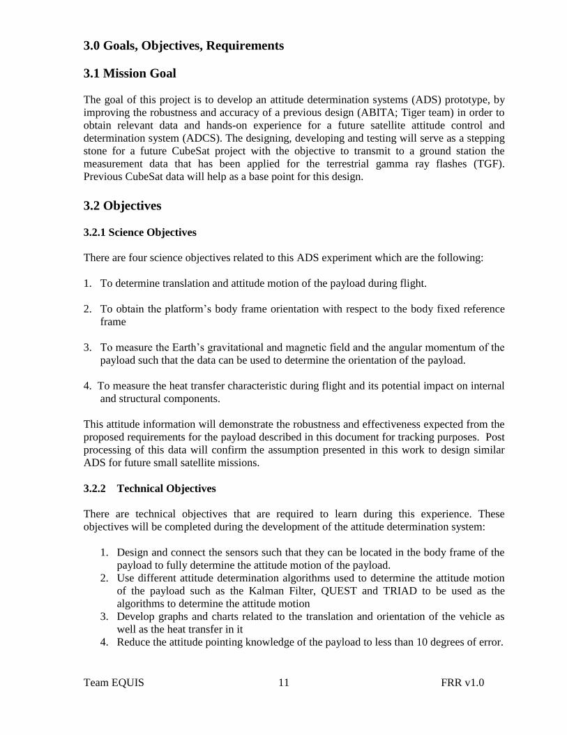
3.0 Goals, Objectives, Requirements
3.1 Mission Goal
The goal of this project is to develop an attitude determination systems (ADS) prototype, by
improving the robustness and accuracy of a previous design (ABITA; Tiger team) in order to
obtain relevant data and hands-on experience for a future satellite attitude control and
determination system (ADCS). The designing, developing and testing will serve as a stepping
stone for a future CubeSat project with the objective to transmit to a ground station the
measurement data that has been applied for the terrestrial gamma ray flashes (TGF).
Previous CubeSat data will help as a base point for this design.
3.2 Objectives
3.2.1 Science Objectives
There are four science objectives related to this ADS experiment which are the following:
1. To determine translation and attitude motion of the payload during flight.
2. To obtain the platform’s body frame orientation with respect to the body fixed reference
frame
3. To measure the Earth’s gravitational and magnetic field and the angular momentum of the
payload such that the data can be used to determine the orientation of the payload.
4. To measure the heat transfer characteristic during flight and its potential impact on internal
and structural components.
This attitude information will demonstrate the robustness and effectiveness expected from the
proposed requirements for the payload described in this document for tracking purposes. Post
processing of this data will confirm the assumption presented in this work to design similar
ADS for future small satellite missions.
3.2.2 Technical Objectives
There are technical objectives that are required to learn during this experience. These
objectives will be completed during the development of the attitude determination system:
1. Design and connect the sensors such that they can be located in the body frame of the
payload to fully determine the attitude motion of the payload.
2. Use different attitude determination algorithms used to determine the attitude motion
of the payload such as the Kalman Filter, QUEST and TRIAD to be used as the
algorithms to determine the attitude motion
3. Develop graphs and charts related to the translation and orientation of the vehicle as
well as the heat transfer in it
4. Reduce the attitude pointing knowledge of the payload to less than 10 degrees of error.

Team EQUIS 12 FRR v1.0
These objectives provide the desire knowledge to learn how the attitude determination
system can be used in an actual mission.
3.3 Science Background and Requirements
3.3.1 Science Background
The design of the attitude determination system (ADS) for this payload is a midpoint
development for a future CubeSat project with the purpose of communicating data about
measurements for science missions such as a terrestrial gamma ray flashes (short blasts of
gamma rays, which are discharged from the uppermost part of the atmosphere into space1) or
other similar science objectives. The intended requirements must be those needed for an
effective and almost error free communication of the ADS data for the CubeSat that will be
navigating at a height above the Earth’s surface as well as the design of the communication
system with a suitable main lobe beamwidth. The A.D.S. project will give the opportunity to
enhance the chosen technology as well as determine the minimum adjustments that it might
need to meet the goal, which is to develop an attitude determination system prototype.
The attitude of a spacecraft is its orientation in space. The motion of a rigid spacecraft is
specified by its position, velocity, attitude, and attitude motion. The position, acceleration,
and velocity quantities describe the translational motion of the center of mass of the spacecraft
and can be determined from previously defined spatial frames such as the magnetic field of
the Earth and the moment of inertia of the body itself. Moreover, attitude determination is
used to change the spacecraft’s direction and maintain the spacecraft on-course (Attitude
Control System).
Attitude analysis can be classified in three types: attitude determination, prediction, and
control. Attitude determination is a process of calculating the orientation of an object relative
to an inertial reference frame. Attitude prediction is the process of anticipating the future
course of the object through the analysis of dynamic models to extrapolate the attitude history.
Attitude control is the method of controlling the orientation of the object based on a
predetermined data from the sensors; it consists of two areas of control, attitude stabilization
and maneuver control, for example a CubeSat project.
The orientation of the payload will be determined by comparing its actual three axis body
frame (three dimensional orthogonal axes at the payload center of mass) with those of three
external vector fields: the Earth’s gravitational field, the payload angular momentum, and the
Earth’s magnetic field.
The gravitational field will serve as a reference frame to measure the change of position,
velocity and acceleration of the payload. The gravitational field has a constant direction
(towards the Earth’s center) which allows its use as a trusted reference frame. The change of
the payload’s center of mass with respect to the Earth’s gravitational frame is done by
determining the yaw, pitch, and roll of the payload when its acceleration is determined with
1 The gamma rays are presumed to be released by electrons traveling at the speed of light when they scatter off
of atoms and decelerate. The mechanism in which the electrons produce TGFs is uncertain; although, it
probably involves the build-up of electric charge at the tops of clouds due to lightning discharge. This results in
a powerful electric field between the top of the clouds and the ionosphere. (Tim Stephens, UC at Santa
Cruz,2005)

Team EQUIS 13 FRR v1.0
respect to the gravitational field. A single integration of the acceleration will have a result of
the payload’s velocity (a vector) and a double integration will result in the payload’s position
with respect to a previous measured point (previous state or reference starting point).
Figure 1: Three axis center mass reference frame and their rotational change definition
Figure 1 illustrates the rotational movements (roll, pitch, and yaw), which are described in
reference to a plane. The movement described is a combination of two-axis (2 dimensional)
area and a missing combination of a pair of axis (pitch) is portrayed in the z – y plane. The
acceleration with respect to the gravitational field will determine the proper acceleration,
which is the acceleration “detected” by the payload within the reference gravitational field.
For example, the gravitational field strength is 1g; the proper acceleration of the payload must
be obtained by subtracting this 1g to that acceleration sensed. If the velocity is constant the
proper acceleration is zero (0).
The ABITA project (2008), determined the balloon dynamics during flight by doing the
following: comparing acceleration vs. altitude, rotational rate, and translational movement of
the payload. The ABITA payload used the gravitational field to determine its acceleration. A
known disadvantage of using the aforementioned is that it needs another frame to initialize the
spatial model (such as data from a GPS). As a brief description of its basic operation, to
measure acceleration is to determine the vibration, or acceleration of motion of a structure.

Team EQUIS 14 FRR v1.0
Figure 2: Accelerometer average values
As it is observed from Figure 2 the average maximum and minimum acceleration that was
achieved by the ABITA was approximately 1.6g and -1.2g, respectively. The values shown
on Figure 3, repeat at 3g, thus it is considered the maximum average.
Figure 3: Accelerometer maximum values
In conjunction with measuring the acceleration, the measurement of the moment of inertia is
used to determine accurately the attitude of the payload. The angular momentum of the
payload and its rate of change, with respect to time, provide information of the payload’s
orientation state in a repetitive measured time frame. There is an equivalence between the
angular momentum at a specific distance from the center of a spinning body (r), the moment
of inertia (I), the angular speed (), and linear momentum (p) that a body experiments when
moving in a straight line at a known velocity (v). The moment of inertia is defined as the
resistance of a body to an angular acceleration applied to it. The resistance to the angular
acceleration, on any of the 3 rotational axes, can be measured to determine when the body is
rotating due to an external applied force. The result of the integral of an angular acceleration
Team EQUIS 15 FRR v1.0
is the velocity and position of the body. The initial position is obtained by using other
reference information, such as that obtained from a Global Positioning System.
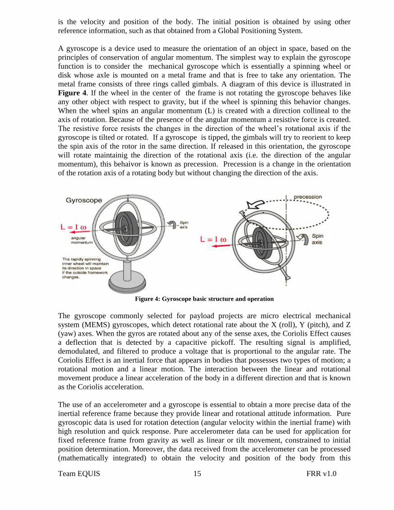
A gyroscope is a device used to measure the orientation of an object in space, based on the
principles of conservation of angular momentum. The simplest way to explain the gyroscope
function is to consider the mechanical gyroscope which is essentially a spinning wheel or
disk whose axle is mounted on a metal frame and that is free to take any orientation. The
metal frame consists of three rings called gimbals. A diagram of this device is illustrated in
Figure 4. If the wheel in the center of the frame is not rotating the gyroscope behaves like
any other object with respect to gravity, but if the wheel is spinning this behavior changes.
When the wheel spins an angular momentum (L) is created with a direction collineal to the
axis of rotation. Because of the presence of the angular momentum a resistive force is created.
The resistive force resists the changes in the direction of the wheel’s rotational axis if the
gyroscope is tilted or rotated. If a gyroscope is tipped, the gimbals will try to reorient to keep
the spin axis of the rotor in the same direction. If released in this orientation, the gyroscope
will rotate maintainig the direction of the rotational axis (i.e. the direction of the angular
momentum), this behaivor is known as precession. Precession is a change in the orientation
of the rotation axis of a rotating body but without changing the direction of the axis.
Figure 4: Gyroscope basic structure and operation
The gyroscope commonly selected for payload projects are micro electrical mechanical
system (MEMS) gyroscopes, which detect rotational rate about the X (roll), Y (pitch), and Z
(yaw) axes. When the gyros are rotated about any of the sense axes, the Coriolis Effect causes
a deflection that is detected by a capacitive pickoff. The resulting signal is amplified,
demodulated, and filtered to produce a voltage that is proportional to the angular rate. The
Coriolis Effect is an inertial force that appears in bodies that possesses two types of motion; a
rotational motion and a linear motion. The interaction between the linear and rotational
movement produce a linear acceleration of the body in a different direction and that is known
as the Coriolis acceleration.
The use of an accelerometer and a gyroscope is essential to obtain a more precise data of the
inertial reference frame because they provide linear and rotational attitude information. Pure
gyroscopic data is used for rotation detection (angular velocity within the inertial frame) with
high resolution and quick response. Pure accelerometer data can be used for application for
fixed reference frame from gravity as well as linear or tilt movement, constrained to initial
position determination. Moreover, the data received from the accelerometer can be processed
(mathematically integrated) to obtain the velocity and position of the body from this

Team EQUIS 16 FRR v1.0
previously reference starting point. Having both gyroscopes and accelerometers we can obtain
the motion processing solution of linear movement and rotation at the same time. By tracking
both the current angular velocity of the system and the current linear acceleration of the body
it is possible to determine the overall attitude, position, and velocity of the body provided by a
starting reference point in time (for example, determined periodically from a GPS). The
starting point provided by the reference mechanism (GPS) provides for the minimization of
the cumulative errors inherent of a sensors system with no external reference frame used when
integration is used.
The Earth’s magnetic field is used as a reference frame for the payload in order to determine
attitude. The magnetic field exists due to the movement inside the Earth’s liquid in the outer
core (mostly compound by iron) that produces an electric current. A dynamo effect is created
and it converts the Earth to a very large bar magnet with a magnetic field that goes from the
North Pole to the South Pole associated to it. Figure 5 presents a not-to-scale representation
of the magnetic field. The HASP mainframe should rise at about 120,000 feet or
approximately 36 km navigating through the magnetic field.
Figure 5: Earth's Magnetic Field
Earth has a magnetic field tilted at about 23.5º with respect to the rotational (physical) axis.
The common sensor used to detect this magnetic field reference frame is the magnetometer.
The magnetometer that will be used for the A.D.S. project consists of three axes (x, y, and z)
that will provide a vector component. The data obtained from this device will be the magnetic
field intensity vs. typical values of the Earth’s magnetic field that goes from 30,000 nT (in the
equator) towards 60,000 nT (in the Poles). Typical values of a magnetometer suitable for this
payload are approximately ±1,000,000 nT and ±15 nT of resolution. The magnetic field vector
will be obtained by the combination of the measurements of each axis and thus can be
projected with respect to the Earth’s magnetic field to determine the payload’s orientation. In
attitude determination systems magnetometers are used because of vector sensing capabilities.
They can provide both direction and magnitude of the magnetic field.

Team EQUIS 17 FRR v1.0
Figure 6: Magnitude of the earth’s magnetic field
The Earth's magnetic field can be described, at any point and time by a direction and intensity
which can be measured. The Earth’s magnetic field is a vector field in which at least three
components are necessary to represent the field. Commonly the components of the
geomagnetic field that are measured are the north (X) and east (Y) components of the
horizontal intensity and the vertical intensity (Z). From these elements, all other parameter of
the magnetic field can be calculated. A figure that illustrates these parameters is the following:
Figure 7: Parameters of the magnetic field
The magnetic field’s direction is described by the declination (D) and the inclination (I).
These two parameters (i.e. D and I), are measured in units of degrees. The declination angle is
form between the magnetic north (i.e. x in the plot), and the horizontal intensity or true north.
The inclination angle is form between the horizontal intensity and the total intensity field
vector. The parameters that describe the field intensity are the total intensity (F), horizontal
component (H), vertical component (Z), and the north (X) and east (Y) components of the
horizontal intensity. These parameters are normally expressed in units of nanoTesla or gauss.
The magnetic field parameters measured are used to determine the payload’s orientation with
respect to the axis directions of the Earth’s magnetic field. (i.e. Northward Eastward and
Downward in the figure #). To explain the procedure performed to interpret the magnetometer
data in order to define the payload’s orientation let’s consider the following example:
Team EQUIS 18 FRR v1.0
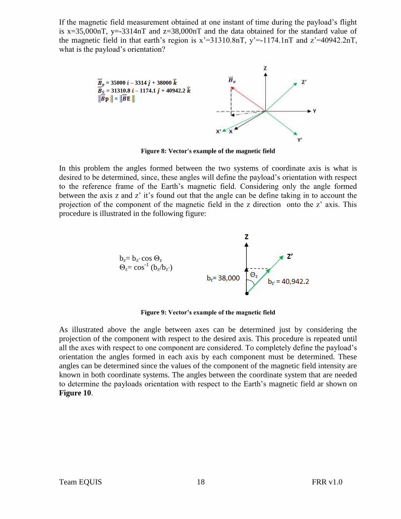
If the magnetic field measurement obtained at one instant of time during the payload’s flight
is x=35,000nT, y=-3314nT and z=38,000nT and the data obtained for the standard value of
the magnetic field in that earth’s region is x’=31310.8nT, y’=-1174.1nT and z’=40942.2nT,
what is the payload’s orientation?
Figure 8: Vector's example of the magnetic field
In this problem the angles formed between the two systems of coordinate axis is what is
desired to be determined, since, these angles will define the payload’s orientation with respect
to the reference frame of the Earth’s magnetic field. Considering only the angle formed
between the axis z and z’ it’s found out that the angle can be define taking in to account the
projection of the component of the magnetic field in the z direction onto the z’ axis. This
procedure is illustrated in the following figure:
Figure 9: Vector’s example of the magnetic field
As illustrated above the angle between axes can be determined just by considering the
projection of the component with respect to the desired axis. This procedure is repeated until
all the axes with respect to one component are considered. To completely define the payload’s
orientation the angles formed in each axis by each component must be determined. These
angles can be determined since the values of the component of the magnetic field intensity are
known in both coordinate systems. The angles between the coordinate system that are needed
to determine the payloads orientation with respect to the Earth’s magnetic field ar shown on
Figure 10.
p = 35000 – 3314 + 38000
E = 31310.8 – 1174.1 + 40942.2
=
bz= bz’ cos Θz
Θz= cos-1
(bz/bz’)

Team EQUIS 19 FRR v1.0
Figure 10: Angles of interest
Therefore three equations are necessary to completely define the payload’s orientations since
three angle are needed to define the payload’s attitude. These equations are:
Θz= cos-1
(bz/bz’) Θy= cos-1
(by/by’) Θx= cos-1
(bx/bx’)
The value of the earth’s magnetic field in a certain region of the earth will be provided by
simulation software available in the International Geomagnetic Reference Field (IGRF) web
page. This simulator only request values of altitude, latitude and longitude to estimate the
magnitude and direction of the earth’s magnetic field. The latitude, longitude and altitude
information will be provided by the GPS on board the HASP platform to perform the analysis
post flight.
Post processing of the received data might include the use of mathematical and statistical
algorithms such as the Kalman Filter, to decrease substantially inherent noise in the data. This
allows predicting the real position and orientation of the payload at any moment during flight.
The Kalman Filter determines the next state estimation by using average weighted matrices
that combines the present state, a mathematical model of the measurement systems and the
noise inherent to both, the system and the measurement devices.
The position and direction of movement will be obtained by determining the payload’s current
position, velocity, and acceleration. The x(t), y(t), and z(t)) will be recorded periodically in a
pre-defined time rate for the whole flight trajectory (creating a vector matrix of its position,
x(t+nt), y(t+nt), z(t+nt), where i stands for the predefined time slot and n stands for a counter
with a limit).
)().......4()3()2()( 3210 nttxtxtxtxtxX n
)().......4()3()2()( 3210 nttytytytytyY n
)().......4()3()2()( 3210 nttztztztztzZ n

Team EQUIS 20 FRR v1.0
A matrix is constructed with the x-y-z axes. Noise suppressor and position predictor
algorithms are used with matrix base mathematical operations to “recover” the real position
from the raw data (typical from the sensing elements inaccuracies) and a 3-dimensional
trajectory diagram.
According to the flight operation plan provided in the HASP website; the platform will launch
at a rate of about 1000 feet per minute. Thus, with this ascent velocity is expected that the
payload reach the float altitude (i.e. 120,000 feet) in approximately 1 ½ to 2 hours. The actual
flight profile for the 2006 HASP flight is shown in Figure 11.
Figure 11 is a comparison between
a HASP flight (blue curve) and the
profile for typical latex, sounding
balloon flight (red curve). The
vehicle will stay at an altitude (i.e.
at the stratosphere) for about 5 to 15
hours before the flight must be
terminated to parachute HASP into
a safe landing zone.
The trajectory expected for the
HASP payload, considering Figure
11, can be divided in two phases:
that of a turbulent launch and that
of a steady and slow dynamic
behavior. Figure 12 illustrates the
payload’s trajectory, when the payload ascends up to 120,000 feet in two approximately 2
hours and when it reaches a near constant altitude for a time greater than 15 hours but no more
than 18 hours.
The first phase data will
be used to determine the
gradient of temperature
in the physical structure
of the payload and the
possible impact it may
have in the performance
of the internal electronic
components and
subsystems.
A typical communication
link for a small satellite,
in LEO (Low Earth
Orbit), with an antenna
beamwidth of 30, a
height of 700 km, and an average speed of 7,500 km/s will need an approximate time of 22
minutes to pass over the ground station communication.
Figure 11: HASP 2006 flight profile
Figure 12: Payload trajectory dynamics

Team EQUIS 21 FRR v1.0
This is justified by
developing the
following analysis. For
an average Earth radius
plus the height of the
satellite of 7,078 km
(6,378 km + 700 km)
and at the speed of
7,500 km/s the linear
displacement in orbit in
1 minute will be of:
In the preceding calculation s stands for a segment of the circumference that the satellite will
travel in one (1) minute. Then, the angle of translation is determined as follows (s is
approximate as a line but it is really a
segment of a circumference):
1000,078,7
000,125sinsin 1
r
s
Then, at the speed of 7,500 km, the satellite
will travel about 1.
Since the downlink antenna beamwidth chosen is about 30 degrees the angle from the
maximum power density center of the mainlobe and the -3 dB (half of power density) is 15.
In order to assure a robust communication link a 20 angle is chosen. Then the needed
minimum accuracy for orientation used will be 10.
The downlink antenna beamwidth
chosen can also be employ to
determine the accuracy of the
position desired for this project. To
define the position’s accuracy two
important cases must be
considered. One is the movement
of a cube sat along its orbit and the
second is the effect of the orbit
decay in the strength of the
downlink communication signal. In
order to define correctly the
accuracy of the position the most
limiting case for the downlink
communication must be examined. This limiting case occurs when the satellite is pointing
Figure 13: Angle of translation determination
min/000,125
min1
60
1
/500,7ms
ssm
Figure 14: Angle of translation determination
Figure 15 Beamwidth shade diameter determination

Team EQUIS 22 FRR v1.0
directly downward, because is in this orientation where the signal covers less distance in
comparison with other types of orientations. If a height of 400 km out of the earth’s
atmosphere is considered for the cubesat’s orbit and a beamwidth of 300, the distance covered
by that situation is of 214 km. The visualization and procedure follow to determine this
distance is shown in the following figure:
Figure 16: Determining position accuracy
This implies that if a 3db of power density don’t want to be lost in the communication link at
least an accuracy of a 100 km should be used for the position. If the effect of orbit decay in
the strength of the downlink communication signal is examined considering that at least 100
km have been lost it’s found that the 214 km of covered distance from the previous case (i.e
400 km of height), have been reduce to approximately 160 km. This means that the second
case suggests a smaller value of position accuracy do to the effect of the cubesat’s orbit decay,
therefore it can be concluded that the lost in altitude will be the limiting factor to establish the
accuracy of the position.
Figure 17: Determining position accuracy with orbit decay
An examination of previous data must be employ to completely define the accuracy of the
position considering the phenomena of orbit decay. That is why data of orbit decay is
retrieved from the Department of Industry Tourism and Resources to complete this task. This
data is illustrated in the following figure:
Team EQUIS 23 FRR v1.0
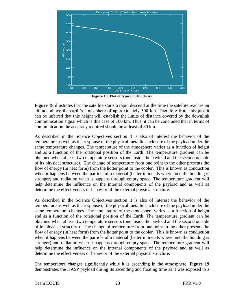
Figure 18: Plot of typical orbit decay
Figure 18 illustrates that the satellite starts a rapid descend at the time the satellite reaches an
altitude above the earth’s atmosphere of approximately 300 km. Therefore from this plot it
can be inferred that this height will establish the limits of distance covered by the downlink
communication signal which is this case of 160 km. Thus, it can be concluded that in terms of
communication the accuracy required should be at least of 80 km.
As described in the Science Objectives section it is also of interest the behavior of the
temperature as well as the response of the physical metallic enclosure of the payload under the
same temperature changes. The temperature of the atmosphere varies as a function of height
and as a function of the rotational position of the Earth. The temperature gradient can be
obtained when at least two temperature sensors (one inside the payload and the second outside
of its physical structure). The change of temperature from one point to the other presents the
flow of energy (in heat form) from the hotter point to the cooler. This is known as conduction
when it happens between the particle of a material (better in metals where metallic bonding is
stronger) and radiation when it happens through empty space. The temperature gradient will
help determine the influence on the internal components of the payload and as well as
determine the effectiveness or behavior of the external physical structure.
The temperature changes significantly while it is ascending in the atmosphere. Figure 19
demonstrates the HASP payload during its ascending and floating time as it was exposed to a

Team EQUIS 24 FRR v1.0
very extreme environment that consists of very low and high temperatures at a very low
pressure (i.e. 5 – 10 millibars).
Figure 19 illustrates the lowest
temperature that was found on
the platform’s top was of -80 0C and could be lower due to
the form of the curve. The
highest temperature
encountered during the 2006
HASP flight was of
approximately 40 0C. The
exposure to these
environmental conditions is
what makes necessary the
design of a thermal control
system so that the electronic
equipment inside the payload can be kept working at its optimal temperature range.
The description of the ADS above, including the chosen attitude determination reference
frames are intended for a robust and precise control of satellite for ground station contact. In
order to test the proposed operation of the ADS, the collection of data needs to be done with
adequate technology. The data collected will determine the attitude of the payload within the
abovementioned reference frames. Proper design and programming of hardware components
and sub-systems are intended to record the relevant data that will be post-processed to
determine the tracking of the payload during the whole test flight.
3.3.2 Science Requirements
To accomplish the development of a robust ADS prototype that would be used to determine
the orientation of a satellite, it is necessary to define the requirements that are needed to obtain
the orientation, position and heat characteristics of the payload throughout the flight. These
requirements are:
1. Determine the payload position within accuracy of 80 km.
2. Determine the heat transfer rate into or out of the payload.
3. Verify the orientation of the payload by comparing an external reference magnetic
field and the International Geomagnetic Reference Field (IGRF) model of the year
2010.
4. Use and verify the position accuracy of the Inertial Measurement Unit (IMU) with
respect to the position GPS data.
5. Use the obtained data to gather knowledge about the attitude motion of the payload
and provide recommendations for future HASP and CubeSat projects.
6. Complete final science report post flight.
Figure 19: Temperature variation during flight

Team EQUIS 25 FRR v1.0
3.4 Technical Background and Requirements
3.4.1 Technical Background
The ADS developed in this project consists of several sensors and a data processing unit used
to collect and store the measurements needed to determine the payload’s position and
orientation at intervals of time during the flight. The ADS is use to determine the payload’s
attitude, using different reference frames that will be established by the following equipment:
Accelerometer
For application with space and weight limitations there are three different kinds of
accelerometers commonly used which are the piezoelectric micro-accelerometer,
capacitive micro-accelerometer and the tunneling current micro-accelerometer. The
type of accelerometer selected for this application is the piezoelectric micro-
accelerometer. It has been selected because its measures are not affected by parasitic
capacitance or electromagnetic interference (EMI) which is disadvantages of
capacitive accelerometers. In addition piezoelectric accelerometers don’t require a
high voltage like the tunneling current accelerometer. The piezoelectric accelerometer
selected is an electromechanical device that obtains acceleration using the relation that
exists between a piezoelectric deformation and the rate of change of the velocity in the
body. When the body of the system accelerates a force is created and this force
produce a deformation in the small piezoelectric that form part of the sensor. The
principle of operation of these devices is presented in the following Figure 17.
Figure 20: Accelerometers basic principal of operation
As the body moves the mass in the sensor due to its inertia moves in the vertical
direction producing a deformation in the beam. The piezoelectric is embedded in the
location of the beam’s maximum deflection and is that deformation which affects the
piezoelectric producing a change in the piezoelectric structure. This piezoelectric
deformation causes a change in the piezoelectric resistance that consequently will alter
the output voltage of the piezoelectric of the specific axis where this inertial change
occurs. This amount will permit us to determine the linear acceleration of the payload
during the flight. This device will allow us to understand the payload behavior better,
thus allowing better knowledge of payload’s motion. An average sensitivity of
10mV/g is commonly encountered in this type of sensors.

Team EQUIS 26 FRR v1.0
Gyroscope
The three-axis gyroscope is a device for measuring the payload’s degree of rotation.
The types of gyroscopes commonly used for applications with space limitations are the
Micro Electrical Mechanical System (MEMS) gyro. These types of gyroscopes are
compose by miniature mechanical elements that vibrates and electronic components
used to process the data produced by the mechanical elements. The vibration of the
mechanical element is affected every time the payloads rotate due to the Coriolis effect
(see section #), which produce a vibration in direction different to direction of the
initial vibration. This resultant vibration is directly related to the angular velocity of
the payload’s rotation. This second vibration is sensed and processed by the electronic
equipment in the gyroscope to finally determine the payload’s angular velocity
readings. To illustrate the principal of operation of these devices consider the
following figure:
Figure 21: Gyroscopes basic principal of operation
The gyroscope readings will provide information about the payload’s rotation on each
one of the axes. The gyroscope and accelerometer data can be combined to acquire a
more precise measure of the payload’s orientation.
Three-axis magnetometer
The ADS system of the payload will take measurements of the strength of the Earth’s
magnetic field. These measurements will be used to obtain the position of the payload
during the complete flight. The magnetometer detects the magnitude of the earth’s
magnetic field on each axis, in this case; X, Y and Z. To obtain the magnetic field the
magnetometer works by measuring the magnetic filed through magneto inductance by
using a circuit that is magneto inductive (which consist of a coil around a
ferromagnetic core). A relaxation oscillator connected to this magnetic circuit works
by gradually building up charge in the circuit and discharging rapidly, this cycle
repeats itself. As the strength of the magnetic field varies so does the frequency of
oscillation in the coil that is perpendicular to field. The output of the magnetometer is
in form of a square wave signal that can be read as a digital signal. This output

Team EQUIS 27 FRR v1.0
represents the magnitude of the magnetic field on a specific axis; having three
magnitudes will allow the calculation of the earth magnetic field vector.
Figure 22: Simplified representation of magnetometer basic operations
The magnetic field is directly related to the cosine of the angle; as a result, when the
angle changes, the magnetic field will change will result in a change of voltage at the
output of the sensor. The following equation represents the relationship between the
magnetic field and the angle at different times.
Where and is the magnetic constant field. Note that the output of the
magnetometer is measured in volts depending directly on the strength of the field
along the axis. Three different circuits as described above would be needed if three
dimensional frame detection is desired.
Temperature sensor
Different kinds of temperature sensors have been develop in the present to meet
diverse kind of requirements that can appear in a variety of applications. These sensors
differ in their ranges of measurements, sensitivity, accuracy, and mode of sensing. The
different kinds of temperature sensor that exist today can be classified as
thermocouples, thermistors, RTD’s, or solid state sensors. For this application the
temperature device considered is solid state sensor. An illustration of this type of
sensor is presented in the following figure:
B
B component along coil axis
Team EQUIS 28 FRR v1.0
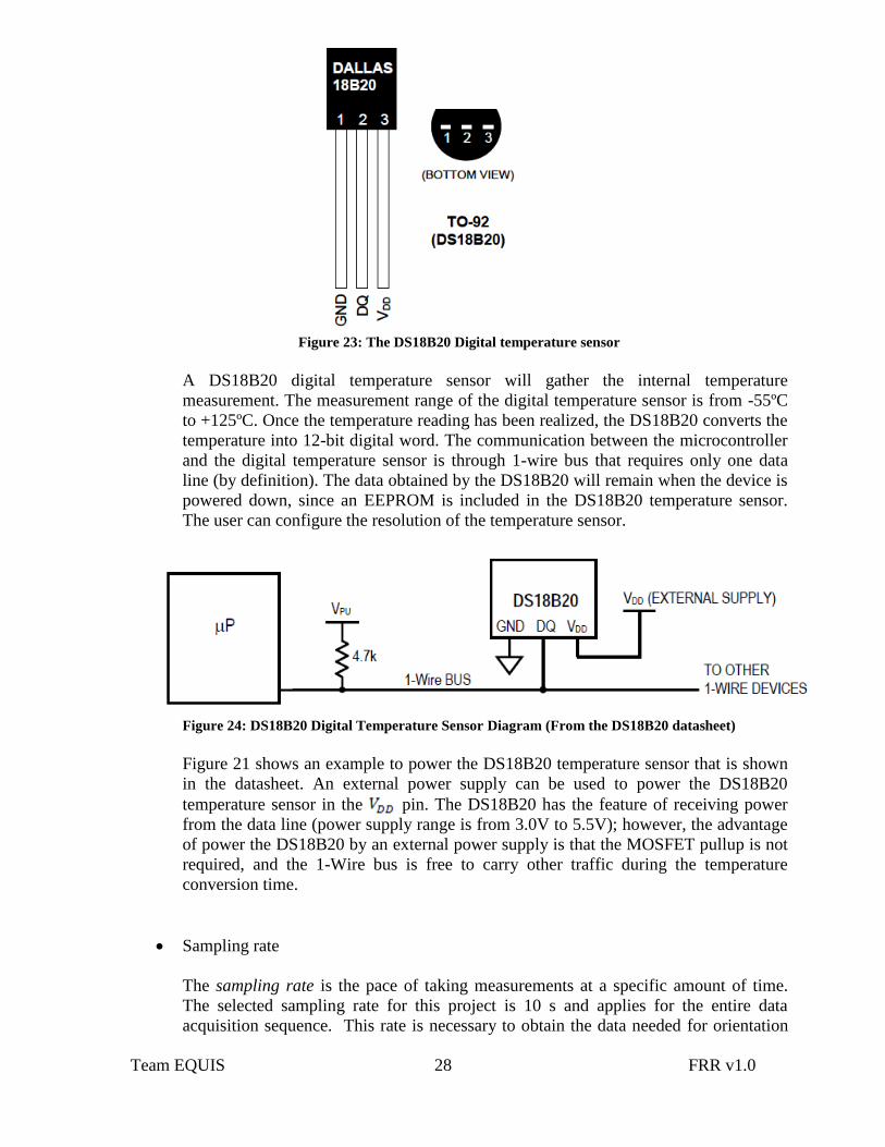
Figure 23: The DS18B20 Digital temperature sensor
A DS18B20 digital temperature sensor will gather the internal temperature
measurement. The measurement range of the digital temperature sensor is from -55ºC
to +125ºC. Once the temperature reading has been realized, the DS18B20 converts the
temperature into 12-bit digital word. The communication between the microcontroller
and the digital temperature sensor is through 1-wire bus that requires only one data
line (by definition). The data obtained by the DS18B20 will remain when the device is
powered down, since an EEPROM is included in the DS18B20 temperature sensor.
The user can configure the resolution of the temperature sensor.
Figure 24: DS18B20 Digital Temperature Sensor Diagram (From the DS18B20 datasheet)
Figure 21 shows an example to power the DS18B20 temperature sensor that is shown
in the datasheet. An external power supply can be used to power the DS18B20
temperature sensor in the pin. The DS18B20 has the feature of receiving power
from the data line (power supply range is from 3.0V to 5.5V); however, the advantage
of power the DS18B20 by an external power supply is that the MOSFET pullup is not
required, and the 1-Wire bus is free to carry other traffic during the temperature
conversion time.
Sampling rate
The sampling rate is the pace of taking measurements at a specific amount of time.
The selected sampling rate for this project is 10 s and applies for the entire data
acquisition sequence. This rate is necessary to obtain the data needed for orientation
Team EQUIS 29 FRR v1.0
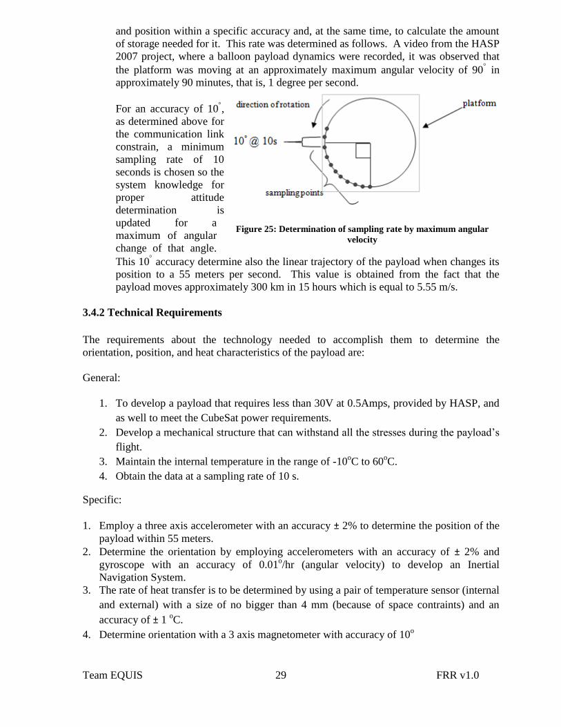
and position within a specific accuracy and, at the same time, to calculate the amount
of storage needed for it. This rate was determined as follows. A video from the HASP
2007 project, where a balloon payload dynamics were recorded, it was observed that
the platform was moving at an approximately maximum angular velocity of 90 in
approximately 90 minutes, that is, 1 degree per second.
For an accuracy of 10,
as determined above for
the communication link
constrain, a minimum
sampling rate of 10
seconds is chosen so the
system knowledge for
proper attitude
determination is
updated for a
maximum of angular
change of that angle.
This 10 accuracy determine also the linear trajectory of the payload when changes its
position to a 55 meters per second. This value is obtained from the fact that the
payload moves approximately 300 km in 15 hours which is equal to 5.55 m/s.
3.4.2 Technical Requirements
The requirements about the technology needed to accomplish them to determine the
orientation, position, and heat characteristics of the payload are:
General:
1. To develop a payload that requires less than 30V at 0.5Amps, provided by HASP, and
as well to meet the CubeSat power requirements.
2. Develop a mechanical structure that can withstand all the stresses during the payload’s
flight.
3. Maintain the internal temperature in the range of -10oC to 60
oC.
4. Obtain the data at a sampling rate of 10 s.
Specific:
1. Employ a three axis accelerometer with an accuracy ± 2% to determine the position of the
payload within 55 meters.
2. Determine the orientation by employing accelerometers with an accuracy of ± 2% and
gyroscope with an accuracy of 0.01o/hr (angular velocity) to develop an Inertial
Navigation System.
3. The rate of heat transfer is to be determined by using a pair of temperature sensor (internal
and external) with a size of no bigger than 4 mm (because of space contraints) and an
accuracy of ± 1 oC.
4. Determine orientation with a 3 axis magnetometer with accuracy of 10o
Figure 25: Determination of sampling rate by maximum angular
velocity

Team EQUIS 30 FRR v1.0
5. Determine position from a three axis accelerometer that has an accuracy of ± 2% and a
reference Global Positioning System sensor.
6. Develop an integrated system of sensor such as magnetometer (10o
accuracy)
accelerometer (± 2% ) and gyroscope (0.01o/hr) at a sample rate of 10s.
4.0 Payload Design
The ADS experiment has a sensor subsystem of five main sensors that will take measurements
to study the balloon platform dynamics. The design arrangement for the experiment consist of
rotational sensor, acceleration sensor, magnetic field sensor, and internal temperature sensor
to acquire data at different positions to get exact information about the Attitude of the
payload.
4.1 Principle of Operation
The ADS experiment will take a variety of measurements, such as acceleration, orientation,
temperature, position, and magnetic field. A three axis accelerometer sensor will be use to
obtain the acceleration data which in the post analysis will be used to obtain velocity and
position and will be compare to the GPS data. The magnetic field concentration will be
determined by a three axis magnetometer to obtain the orientation of the payload. Also the
orientation will be determined by a combination of the gyroscope and accelerometer to obtain
robustness. The internal temperature data will be obtained by an internal temperature sensor
used to monitor the payload’s internal environment to see when the temperature limits of the
devices are reached.
4.2 System Design
Mechanical System
Three Axis
Accelerometer
Flight Control
System
Microcontroller
Three Axis
Gyroscope
Three Axis
Magnetometer
Digital
Temperature
Sensor
Real Time
Clock
SD Card MemoryLegend
Data from Clock
Data from the Sensors
Payload Structure
Transmission of
Data
Figure 26: ADS System Design

Team EQUIS 31 FRR v1.0
The system design (Figure 23) shows the elements of the ADS system. The clear blue
connections designate the data exchange between the flight control and the sensors that will
be in the payload. The green line represents communication between the Microcontroller and
the Real Time Clock to obtain time and day data. The data obtained from the sensors will be
saved in the SD card; this communication is represented by the red line. The light gray line
and the mechanical system box represent the ADS payload structure. The temperature sensor
box represents the internal temperature sensor. The power subsystem is explained in more
detail in the sections 4.3.4 power supply and 4.3.5 power budget.
Arduino Pro 328
An Arduino Pro 328 version 3.3V/8MHz
will be used as the flight control computer
for the ADS experiment. Figure 4 shows
328 provides 3.3V and 40 mA on each of
the I/O pins. The clock speed for the 3.3V
version is 8 MHz. The has both SPI and
I2C interface; as a result sensors with SPI
and I2C protocol can communicate with
the Pro 328. As mentioned above, the
accelerometer and the magnetometer
sensors have SPI interface. Both sensors
have a unique pin for their slave select;
therefore, the Pro 328 can send the
instruction via the developed program to
the sensor that is assigned to read once
the data is available. The gyroscope
sensor can communicate with the Pro 328 using the I2C protocol.
SCA-3000-D01
The schematic for the SCA-3000D01 three axis
accelerometer sensor is shown in Figure 28. The SCA-
3000-D01 has a measurement range of + 2g and has an
SPI digital interface. The SEN-08791 Breakout board
includes an SCA3000 and provides 8 pins in this board.
The pins are as follows; VIN, RST, INT, MOSI,
MISO, SCK, CSB and GND. As mentioned in previous
section 4.4.2 Flight Software, for SPI interface the data
transfer consist of a 4 wire interface; MOSI, MISO,
SCK and CSB. The MOSI and MISO pins stand for
master out slave in and master in slave out
respectively. In addition, the SCK stand for serial clock
and is used to synchronize all the devices. Finally, in
order to select this sensor to communicate with the microcontroller instead of the other slaves,
the SCA-3000-D01 includes a CSB chip select that will be activated by the Pro 328
microcontroller when the Pro 328 sends a signal through this pin. The CSB pin is low active.
Figure 27: Arduino Pro 328 3.3V/8MHz schematic
Figure 28: Three Axis Accelerometer
schematic
Team EQUIS 32 FRR v1.0
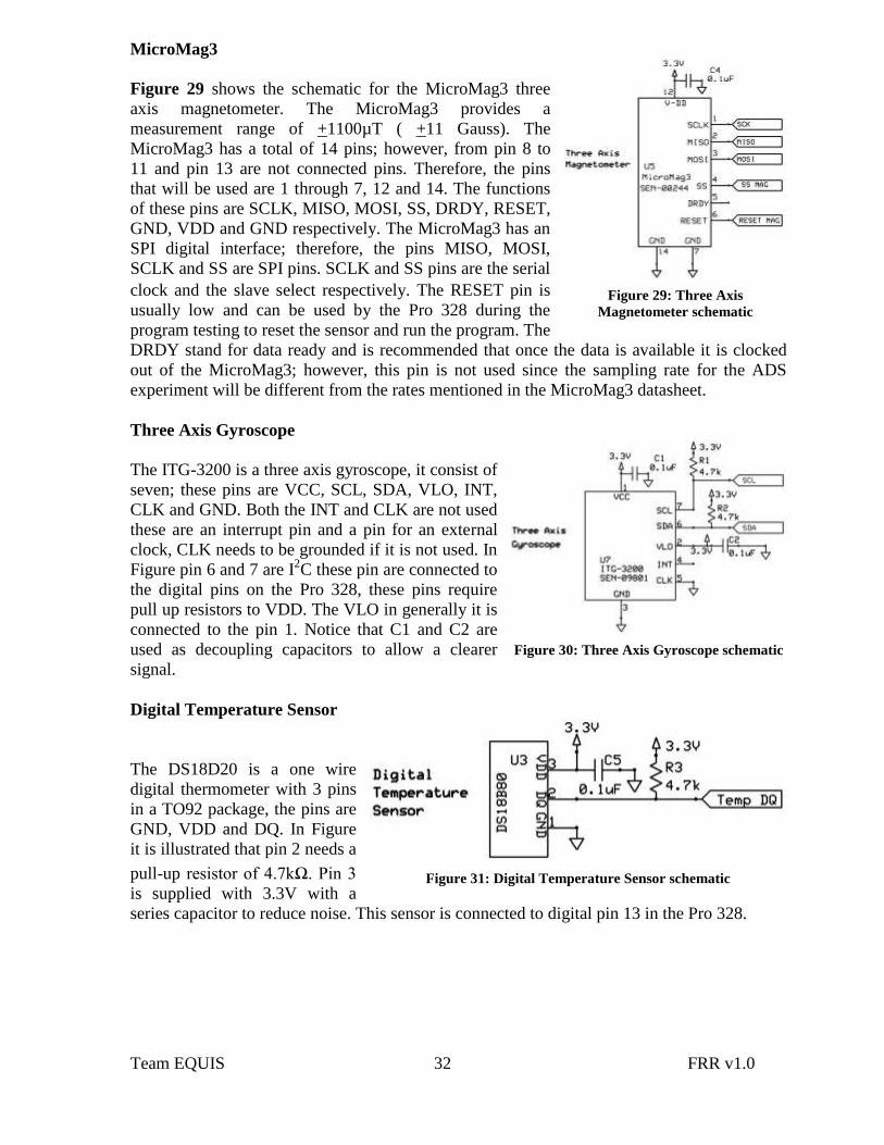
MicroMag3
Figure 29 shows the schematic for the MicroMag3 three
axis magnetometer. The MicroMag3 provides a
measurement range of +1100µT ( +11 Gauss). The
MicroMag3 has a total of 14 pins; however, from pin 8 to
11 and pin 13 are not connected pins. Therefore, the pins
that will be used are 1 through 7, 12 and 14. The functions
of these pins are SCLK, MISO, MOSI, SS, DRDY, RESET,
GND, VDD and GND respectively. The MicroMag3 has an
SPI digital interface; therefore, the pins MISO, MOSI,
SCLK and SS are SPI pins. SCLK and SS pins are the serial
clock and the slave select respectively. The RESET pin is
usually low and can be used by the Pro 328 during the
program testing to reset the sensor and run the program. The
DRDY stand for data ready and is recommended that once the data is available it is clocked
out of the MicroMag3; however, this pin is not used since the sampling rate for the ADS
experiment will be different from the rates mentioned in the MicroMag3 datasheet.
Three Axis Gyroscope
The ITG-3200 is a three axis gyroscope, it consist of
seven; these pins are VCC, SCL, SDA, VLO, INT,
CLK and GND. Both the INT and CLK are not used
these are an interrupt pin and a pin for an external
clock, CLK needs to be grounded if it is not used. In
Figure pin 6 and 7 are I2C these pin are connected to
the digital pins on the Pro 328, these pins require
pull up resistors to VDD. The VLO in generally it is
connected to the pin 1. Notice that C1 and C2 are
used as decoupling capacitors to allow a clearer
signal.
Digital Temperature Sensor
The DS18D20 is a one wire
digital thermometer with 3 pins
in a TO92 package, the pins are
GND, VDD and DQ. In Figure
it is illustrated that pin 2 needs a
pull-up resistor of 4.7kΩ. Pin 3
is supplied with 3.3V with a
series capacitor to reduce noise. This sensor is connected to digital pin 13 in the Pro 328.
Figure 29: Three Axis
Magnetometer schematic
Figure 30: Three Axis Gyroscope schematic
Figure 31: Digital Temperature Sensor schematic

Team EQUIS 33 FRR v1.0
Micro SD Transflash
CD: Card detect
DO: Data output
GND: Ground
SCK: Clock
VCC: Supply Voltage
DI: Data Input
CS: Chip Select
In Figure 32 is demonstrated the Schematic of the SD
Card transflash board with the connections to the
microcontroller. This device has 7 pins CD, DO, GND,
SCK, VCC DI and CS. The serial peripheral interface
(SPI) pins are DI, DO, SCK and CS. As with previous
sensors the capacitor C6 will reduce noise and allow a
clearer signal. Pin 7 is not used when using SPI mode,
pin 7 is mostly used in SD mode.
Serial Alarm Real Time Clock (RTC)
Figure 33 demonstrates the
schematic and pin configuration
use for this experiment. This RTC
is a DS1306 and it is use to obtain
a time stamp. The pins used will
allow to obtain the time without
using any alarm features. Pins 3
and 4 are use for the crystal; the
recommended crystal is a
32.768kHz Quartz crystal with a
series resistance of 45kΩ and a
capacitance of 6pF. Pin 10
through 13 are use for SPI. Pin
16, 14 and 9 needs to be connected to the source, the capacitor C7 allows a clear input signal.
A lithium 3V cell is used as a backup battery in pin 2. In this configuration Vcc2 is connected
to pin 8 and GND. This device is connected to the digital pins in the Pro 328 for SPI.
9V DC to DC
Converter
Connected to the 9V
DC to DC converter
is the power
supplied by HASP
which is 30V @
500mA as shown in
Figure: through
pins 1 and 2. A 3A
diode is used to
Figure 32: MicroSD board schematic
Figure 33: Real-Time Clock schematic
Figure 34: 9V DC to DC Converter schematic

Team EQUIS 34 FRR v1.0
avoid any damage to the devices if a wrong connection is done. The C8 through C11 and C14
is to reduce noise and to guarantee the full parametric performance over the full line and load
range. The 9V output will supply the Pro 328 and the Linear Voltage Regulator. This device
has an efficiency of 80%.
Linear Voltage Regulators
Each one of the sensor and the SD card memory that will
be used for the ADS experiment will be powered by
3.3V. The ADS instruments will receive power from the
HASP platform, which deliver 30V at 0.5 Amps. A 9V
DC to DC converter will transform the 30V provided by
the platform into 9V to power the Pro 328. Since the ADS
electronics (with the exception of the Pro 328 and the DC
to DC converter) will be powered by 3.3V, an
UA78M33IKCS 3.3V linear voltage regulator is required
to reduce the 9V delivered by the DC to DC converter.
The 3.3V linear voltage regulator will remove the excess voltage and it will turn it into heat to
provide the 3.3V.
This device is a linear voltage regulator capable of providing 5V
output for the Real Time Clock since it requires that the input
voltage be higher than 3.2, the device did not work with a input
voltage of 3.3V. The power of the regulator is obtained from the
9V DC to DC converter.
4.2.1 Functional Components
1. Power Subsystem: 0.5 Amps @ 30 VDC will be provided by the HASP platform
during the entire flight. A power budget analysis is required to ensure that this power
will be sufficient for the instruments of the ADS experiment for the entire period of
flight.
2. Microcontroller: The Arduino Pro 328 microcontroller, which is connected to all the
instruments, is in charge of collecting the measurements from all the sensors and stores
it to the memory.
3. SD Card Memory: The SD card memory module will be added to the Arduino were
the measurements of the sensors will be stored here as digital quantities.
4. Three Axes Accelerometer: The accelerometer will take the acceleration
measurements of the payload. Each one of it axes will perform measurements related to
the payload response on that axis.
5. Three Axes Gyroscope: The gyroscope is in charge to determine the orientation of the
ADS payload by sensing the platform rotation during flight.
6. Three Axes Magnetometer: The magnetometer will measure the earth’s magnetic field
intensity.
7. Internal Temperature Sensor: The internal temperature will be monitored by the
flight control computer using an internal temperature sensor. The internal temperature
Figure 35: 3.3V Voltage Regulator
schematic
Figure 36: 5V Voltage
Regulator schematic

Team EQUIS 35 FRR v1.0
readings will be compared with a particular temperature value set in the program of the
microcontroller to identify at what time the maximum temperature is reached.
8. GPS Data: Will provide the position and altitude information of the platform obtained
through HASP website.
9. Mechanical System: The mechanical system is the enclosure of the subsystem
components for the experiment. An aluminum 2014-T4 alloy will be use to construct the
mechanical system to isolate the circuit components and protect them from the
temperature.
10. Thermal Subsystem: The main purpose of the thermal system is to maintain the
internal temperature of the payload within the operating temperature range of the sensors
and the components at the same time protect them from any impact that can damage it.
11. Data Gathering and Analysis: The Pro 328 has to execute the flight software to
gather the sensors measurements and stored it in the SD card. Once the data is extracted
from the SD card several plots will be made to analyze the data and develop new
recommendations.
12. 9V DC to DC Converter: The purpose of this device is to transform the high level
voltage of 30V to 9V to supply the Pro 328 and the linear regulator.
13. 3.3V Linear Voltage Regulator: To supply the sensor with the voltage level of 3.3V it
necessary to use the regulator do to it efficiency with low voltages.
14. 5V Linear Voltage Regulator: To supply the real time clock with the voltage level of
5V it is necessary to use this regulator.
4.2.2 Component Interfaces
The Attitude Determination System will be composed of the following interfaces. The Pro
328 is going to be connected with each one of the sensors output which are digital pins its
interface will be composed of the necessary traces on the PCB. The power subsystem will
have connection with the sensors subsystem and with the Pro 328 to deliver power to both
subsystems, thus permitting for each sensor to receive the power necessary to operate within
the specifications by the use of a 9V DC to DC converter and 3.3V Linear Voltage Regulator.
Also decoupling capacitors will be use to allow a power clearer signal by reducing noise from
the power system. In sections 4.3.3 to 4.3.5 is an explanation in greater detail of the power
interfaces and consumption. The interface between the Magnetometer, Accelerometer and
Gyroscope is a direct connection to the digital pins of the Pro 328. A direct connection
interface with the SD card memory module is used to receive the information that will be
stored. To store the data in micro SD card it is necessary to use a time reference, having the
need for a RTC and its interface is a SPI trace throughout the board.

Team EQUIS 36 FRR v1.0
4.2.3 Traceability
Table 1 below shows the traceability matrix for the ADS experiment.
Main Mission Goal Objectives Requirements Implementation
The goal of this project
is to develop an attitude
determination systems
(ADS) prototype, by
improving the
robustness and
accuracy of a previous
design (ABITA; Tiger
team) in order to obtain
relevant data and
hands-on experience for
a future satellite
attitude control and
determination system
(ADCS). The
designing, developing
and testing will serve as
a stepping stone for a
future CubeSat project
with the objective to
transmit to a ground
station the
measurement data that
has been applied for the
terrestrial gamma ray
flashes (TGF).
Previous CubeSat data
will help as a basepoint
for this design.
To determine
translation and
attitude motion of
the payload during
flight
Determine the
payload position
within accuracy of 10
meters.
Combining the
acceleration and
movements in pitch,
yaw and roll data
from the
accelerometer and
gyroscope
To obtain the
platform’s body
frame orientation
with respect to the
body fixed
reference frame
Determine the
acceleration with an
accuracy of ± 2% and the angular velocity with an accuracy of
0.01o/hr
Employing an
accelerometer with
a resolution of
0.002g and a
gyroscope with a
sensitivity of
14.375 LSB/dps
To measure the
Earth’s
gravitational and
magnetic field and
the angular
momentum of the
payload such that
the data can be
used to determine
the orientation of
the payload.
Determine the
magnetic field with an
accuracy of 10o
Develop an
integrated system
with a
magnetometer with
a resolution of
15nT
Determine the
gravitational field
with an accuracy of ± 2%
Develop an
integrated system
with an
accelerometer with
a resolution of
0.002g
Determine the angular
momentum with an
accuracy of 0.01o/hr
Develop an
integrated system
with a gyroscope
with a sensitivity
of 14.375 LSB/dps
Determine the heat
transfer
characteristic
during flight and
its potential impact
on internal and
structural
components.
Determine the
temperature in the
range of -10 to 60oC
and a accuracy of
0.5%
Use a small signal
diode that can
operate from -30 to
-90oC
Table 1: Traceability Matrix
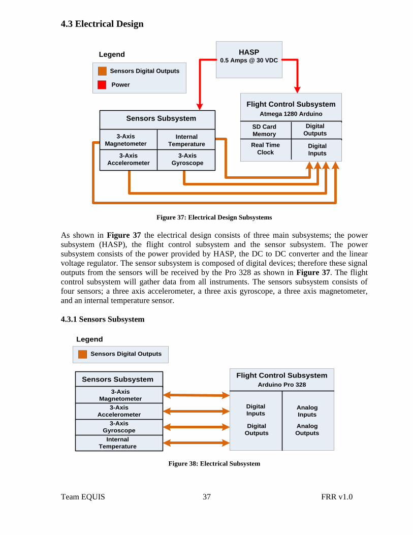
Team EQUIS 37 FRR v1.0
4.3 Electrical Design
Sensors Subsystem
3-Axis
Gyroscope
3-Axis
Accelerometer
3-Axis
MagnetometerInternal
Temperature
Flight Control Subsystem
Atmega 1280 Arduino
SD Card
Memory
Digital
Inputs
Digital
Outputs
Legend
Sensors Digital Outputs
HASP0.5 Amps @ 30 VDC
Power
Real Time
Clock
Figure 37: Electrical Design Subsystems
As shown in Figure 37 the electrical design consists of three main subsystems; the power
subsystem (HASP), the flight control subsystem and the sensor subsystem. The power
subsystem consists of the power provided by HASP, the DC to DC converter and the linear
voltage regulator. The sensor subsystem is composed of digital devices; therefore these signal
outputs from the sensors will be received by the Pro 328 as shown in Figure 37. The flight
control subsystem will gather data from all instruments. The sensors subsystem consists of
four sensors; a three axis accelerometer, a three axis gyroscope, a three axis magnetometer,
and an internal temperature sensor.
4.3.1 Sensors Subsystem
Sensors Subsystem
3-Axis
Gyroscope
3-Axis
Accelerometer
3-Axis
Magnetometer
Internal
Temperature
Flight Control Subsystem
Arduino Pro 328
Digital
Inputs
Digital
Outputs
Legend
Sensors Digital Outputs
Analog
Inputs
Analog
Outputs
Figure 38: Electrical Subsystem

Team EQUIS 38 FRR v1.0
The electrical subsystem is shown in Figure 38 above which allows observing a general view
of how the electrical connections will be done. The sensor subsystem is represented in the left
box and Pro 328 is represented by the right box. The interface between the Pro 328 and each
one of the sensors is represented with the lines with ends. The line ends points at the direction
that the information will be flowing, which is from the sensors to the Pro 328 through the SPI
pins for Magnetometer and the Accelerometer, I2C for the Gyroscope and a digital pins for the
Internal Temperature sensor.
The SCA3000 is a digital three axis accelerometer with an acceleration range of +2 g. The
digital I/O voltage of the SCA3000 is from 1.7 V up to 3.6 V. The digital outputs range of the
SCA3000 accelerometer is from 2.35 V up to 3.6 V.
The sensing element of the SCA3000 three axis
accelerometer consists of three acceleration sensitive masses.
A capacitance change will occur due to acceleration and will
be converted into a voltage change in the signal conditioning
ASIC. The element’s measurement coordinates are rotated
45º compared to the conventional orthogonal X, Y, Z
coordinate system, due to its mechanical construction.
The sensing element is interfaced via a capacitance-to-
voltage (CV) converter. The SCA3000 includes an internal
oscillator, reference and non-volatile memory that enable the sensor’s autonomous operation
within a system. The SCA3000 includes a temperature sensor; therefore, temperature stability
can be reached by using the temperature information from this sensor.
The Figure 40 shows the pins for the SCA3000.
The accelerometer can receive instructions from
the Arduino microcontroller by connecting an
output pin to the accelerometer Master Output
Slave Input (MOSI) pin. The Pro 328 represents
the Master and the accelerometer the slave.
The SCA3000 can be set to operate at low power
to save system level power consumption by using
the Motion Detection (MD) mode. When the Free-
Fall Detection (FFD) is enabled normal
acceleration is available.
The EQUIS team selected the ITG-3200 three axis gyroscope for the ADS experiment. As
mentioned in previous sections, the ITG-3200 is a three axis gyroscope with digital outputs.
The full scale range of the ITG-3200 three axis gyroscope is + 2000 º/s. The ITG-3200 has
digital (I2C) outputs. The operating voltage range of the gyroscope is from 2.1 V up to 3.6 V.
Figure 39: Accelerometer Sensor
Figure 40: SCA3000 Three axis accelerometer
pins

Team EQUIS 39 FRR v1.0
The pins to receive the digital instructions are shown in Figure 29. The ITG-3200 is a three
independent vibratory Micro-electro-mechanical System (MEMs) gyroscope sensitive to
Coriolis forces. The ITG-3200 can detect rotational rate in three axis; the X (roll), Y (pitch),
and Z (yaw).
A rotation about any of the sense axes of the gyro must be induced to create a Coriolis Effect,
which causes a deflection that is detected by a capacitive pickoff. The MEMs device applies
the following process to the detected signal; amplification, demodulation and filtering that
produce a voltage that is digitalized with an internal ADC. The converted voltage is
proportional to the angular rate. The ADC output rate is capable from 3.8 up to a maximum
8,000 sample per seconds, while allowing a wide range of cut off frequencies due to its
capability of a user selectable pass filter.
A MicroMag3 three axis magnetometer has been
selected for the earth’s magnetic field measurements of
the ADS experiment. The three axis magnetometer
sensor operates as an oscillator circuit composed of the
internal sensors, bias, resistors, digital gates and a
comparator. Only one sensor can be measured at the
time. The user sends a command byte to the MicroMag3
through the SPI port specifying the sensor axis to be
measured. A model of the MicroMag3 is shown in
Figure 42.
The micromag3 three axis magnetometer has a low power: draws < 500 µA at 3 VDC and
have a field measurement range (3 VDC at Rb = 43Ω) of +1100 µT. The micromag3 has a
fully digital interface: SPI protocol at 3V, it can also be powered at 3.3V.
A DS18B20 will be the internal temperature sensor for the ADS
experiment. The master (the Pro 328) must issue a convert T
[44h] command in order to initiate a temperature measurement.
The DS18B20 stores the temperature measurement in the 2-byte
temperature register in the scratchpad memory, and then the
DS18B20 will return to its idle state.
Figure 41: Gyroscope Sensor
Figure 42: Three Axis Magnetometer
Figure 43: Digital Temperature
Sensor

Team EQUIS 40 FRR v1.0
The time during flight will be provided by the circuit of an
RTC-Real Time Clock shown in Figure 44. The specific model
will be the DS1306, which can withstand a temperature range
of -40ºC to 85ºC. This device is reliable due to the fact that it
allows to have a backup battery, which in this experiment it
will be a +3V Lithium battery additional to the constant source,
which is 5V. In addition, this device requires a crystal of
32.768 kHz, 6 pF and a resistance of 45 kΩ.
4.3.2 Sensor Interfacing
The sensor connections with the Arduino are as shows the following table;
Sensors Sensors Pins Arduino Pro Pins
Gyroscope (I2C) SCL A4
(I2C) SDA A5
Accelerometer RST 2
SS ACC 3
Magnetometer SS MAG 4
DRDY MAG 5
RESET MAG 6
Digital Temp DQ 7
SD Card SS SD 8
Real Time Clock SS RTC 9
Accelerometer Magnetometer
(SPI) MOSI 10
(SPI) MISO 11
(SPI) SCK 12
Not Connected TBA 13
Not Connected TBA 14
Table 2: Pins for the Pro 328
All the sensors will have an interface between each one of the outputs and the Pro 328. All the
sensors for the ADS experiment are digital sensors; therefore, they do not require any
additional components besides a decoupling capacitor to allow a clearer signal.
Figure 44: Real Time Clock

Team EQUIS 41 FRR v1.0
Figure 45: ADS PCB Design
Figure 45 shows the Print Circuit Board (PCB) design for the ADS experiment. Each one of
the components is represented with yellow lines with its actual size and the corresponding
name. The holes that are required for the PCB to place the components and connect traces
were also realized using the actual size of the leads of each component and are represented
with red circles.
The complete schematic design was linked to the PCB design to enable a tool of the Express
PCB software that indicates the pins that need to be connected according to the schematic.
Several traces were designed on the PCB to realize the required connection between the
components. The green and red lines represent the traces that connect the components in the
PCB. The red lines are the connection traces designed in the top copper layer and the green
lines are the connection traces in the bottom copper layer. When a trace is made in both
copper layers (top and bottom) to make a connection between two components, pass through a
hole to allow connection. Finally, the yellow square that surrounds all the components, holes
and traces represent the actual dimension of the PCB, which is 4 x 4 inches.

Team EQUIS 42 FRR v1.0
4.3.4 Power Supply
30V
3.3V
3.3V9V
5V
3.3V
3.3V
3.3V
30V
9V
HASP
0.5 Amps
at 30 VDC
FUSE Box
9V DC to DC
Converter
Three Axis
Magnetometer
Three Axis
Accelerometer
Three Axis
Gyroscope
Arduino Pro 328
SD Card
Real Time Clock
Digital Internal
Temperature
Sensor
3.3V Linear
Voltage
Regulator
5V Linear
Voltage
Regulator
Figure 46: Power System Diagram
The power subsystem for the ADS experiment is shown in Figure 46. The HASP platform
will be the power source for the ADS experiment and will deliver 30V at 0.5 Amps to the
ADS payload. The fuse shown in the figure 33 is included in the power subsystem to isolate
the ADS electronics from the HASP platform as a safety precaution. As mentioned in the
section 4.2 System Design, a 9V DC to DC Converter will transform the power from the
platform to power the Pro 328. Also a suitable supply of 3.3V is being delivered through a
Linear Voltage Regulator that is represented in the Figure 33 to power the Micro SD board
and all the sensors. Also a 5V voltage converter is used to supply the 5V required for the
RTC.
The Pro 328 has an input voltage range from 3.35V to 12 V; however, the voltage regulator of
the Pro 328 Board may overheat and damage the board when is using more than 12 V and if
the supplied voltage is less than 7 V, the 5 V pin may supply less voltages on the pins and the
board may be unstable [Ref. 14]. Therefore, the Pro 328 will receive 9 V from a DC to DC
converter as shown in Figure 46.

Team EQUIS 43 FRR v1.0
4.3.5 Power Budget
The HASP- High Altitude Student Platform provides power for small and large payloads. For
small payloads the supplied voltage that HASP platform provides is 0.5 Amps @ 30 VDC.
Sensor and Devices Required Voltage
(V)
Required Current
Amperes (A)
Power Consumption
Watts (W)
Power Source
(after HASP) Three Axis Gyroscope
ITG3200 3.3 6.5mA 21.45mW
3.3V Linear
Regulator
Three Axis Accelerometer
SCA3000 3.3 .650uA 21.45uW
3.3V Linear
Regulator
Three Axis Magnetometer
Micromag3 3.3 .500uA 1.65uW
3.3V Linear
Regulator
Digital Temperature Sensor
DS18B20 3.3 1.5mA 4.95mW
3.3V Linear
Regulator
Arduino Pro 328 9 200mA 1800mW 9V DC to DC
Converter
Real Time Clock DS1306 5V 1.28mA 6.4mW 5V Linear
Regulator
SD card circuit 3.3 100mA(max)
40-60mA(Typical) 330mW
3.3V Linear
Regulator
Max consumption of sensors
and devices -- 2162mW --
Table 3: Power Requirements
Table 3 demonstrates the current, voltage required, power source and power consumption for
each of the electronic sensors without the power devices as the linear Regulator and DC to DC
converter. Note that the current consumed by the SD card is a maximum value and that the
typical value is in the range of 40mA to 60mA depending on brands.
The total power consumption was obtained through a mathematical analysis that can be
observe in Figure 47, first all the current of the sensors is sum, then multiplied by the voltage
supplied to obtain the power. This current consumed by the sensor is also consumed by the
linear voltage regulator; to obtain the power dissipated by the regulators, the current
consumed is multiplied by the voltage drop of 5.7V in the 3.3V regulator, and this procedure
is also done with the 5V regulator. The 108mA consumed by the 3.3V regulator, the 1.28mA
consumed by the 5V regulator and the 200mA of the Pro 328 are added to obtain the total
current consumed before the 9V converter; this is defined by Kirchhoff Current Law. This
current of 309mA and the voltage of 9V are used to obtain the power consumed which is
2783.5mW. The DC to DC converter need to supply what is required for the components to
work, the converter has an efficiency of 80%. To obtain the total power consumption of the
value power is divided by the efficiency (0.80) thus obtaining the consumption of the ADS
system which is 3479mW. This power value is divided by the 30V supplied by HASP, thus
obtaining the total current and power consumption. The difference between the powers before
and after of the converter will provide the power dissipation of the device. To verify that the

Team EQUIS 44 FRR v1.0
calculation is correct that total power consumption must be equal to sum of the individual
power consumption of all the devices in the ADS system. Therefore:
Total Power = DC to DC Power + Pro328 Power + Regulator Power + Sensor and Devices Power
3479mW 696mW+ 1800mW+ 615.6mW+ 356.4mW+5.12mW+6.4mW
3.3V Linear
Voltage Regulator
Arduino Pro 328
DC to DC
Converter
80% efficiency
9V 200 mA
1800mW
9V
309.28mA
2783.5mW
Sensors and
Devices
200 mA
696 mW
30V 116mA
3479mWHASP Power
30V @ 500mA
5V Linear Voltage
RegulatorReal Time Clock
3.3V 108mA
356.4mW
5V 1.28mA
6.4mW
108 mA
1.28 mA
5.12 mW
615.6mW
Figure 47: Power Budget Analysis
4.4 Software Design
The data will be retrieved from the sensors and thus the software will be designed to store the
data in the SD card.
4.4.1 Data Format & Storage
The total bytes required for the flight is determined by the quantity of the sensors and the total
bytes of the measurement of the sensor times the hours the payload may remain in flight.
The system has four sensors; three axis magnetometer, three axis gyroscope, three axis
accelerometer, and one for the internal temperature sensor. Each sensor with three axes will
have a total of six bytes and the internal temperature sensor will have a total of two bytes. The
time stamp consists of four bytes, one byte for the hours, one byte for the minutes, one byte
for the seconds, and one byte for the date. In total we have 24 bytes for the whole system. The
sample rate will be of approximately 3 seconds. The data will be received 20 times each
minute. The total bytes for the whole flight will be of about 576,000 bytes.

Team EQUIS 45 FRR v1.0
The total bytes required for the system are:
Byte Description
1-4 Time Stamp
5-6 Accelerometer: X axis
7-8 Accelerometer: Y axis
9-10 Accelerometer: Z axis
11-12 Gyroscope: X axis
13-14 Gyroscope: Y axis
15-16 Gyroscope: Z axis
17-18 Magnetometer: X axis
19-20 Magnetometer: Y axis
21-22 Magnetometer: Z axis
23-24 Internal Temperature Sensor Table 4: Bytes Description
The data will be saved in the SD card. The SD card will be formatted FAT 16 before use. The
program will use the SDFat library to create an object to access Fat16 files in SD cards. The
data will be saved as a comma separated values (CSV) format.
4.4.2 Flight Software
To run the code on the Arduino, the code must have two main functions:
Void setup()
o Will run once, when the Arduino starts
o The pins are set (input or output)
Void loop()
o Is an infinite loop, starts running when setup function finishes
o Runs the rest of the code
The magnetometer, accelerometer, SD card, and the real-time clock use the serial peripheral
interface (SPI) to communicate with the microcontroller. SPI is a synchronous serial
communication with one microcontroller (master) and several devices (slaves). The master
provides the clock signal and activates which device (slave) to receive data from. The SPI
uses 4 lines, the slave select line to activate the device, the serial clock line to synchronize the
data communication, the master-in-slave-out (MISO) line to send data from the slave to the
master, and the master-out-slave-in (MOSI) line to send data from the master to the device.
The SPI communication uses the Atmega’s SPI internal registers. The following are the
registers that will be used:
SPDR - SPI data register
SPCR – SPI control register
SPSR – SPI status register
SPIF – SPI interrupt flag

Team EQUIS 46 FRR v1.0
The control register (SPCR) has 8 bits, each bit is a command.
Bit 7 Bit 6 Bit 5 Bit 4 Bit 3 Bit 2 Bit 1 Bit 0
SPIE SPE DORD MSTR CPOL CPHA SPR1 SPR0
Enables
interrupts
Enables
SPI
If bit = 1
sends
LSB
first, if
bit = 0
sends
MSB
first
If bit = 1
sets
master
mode, if
bit = 0
sets slave
mode
Sets
clock
polarity
Sets
clock
phase
Sets SPI
speed
Sets SPI
speed
Table 5: SPCR bit specification
EQUIS software uses SPI mode 0 for the accelerometer and for the SD card and mode 1 for
the real-time clock. In mode 0 the CPOL and CPHA are set as 0; therefore, the leading edge
of the clock uses a sample on the rising edge (signal low to high) and the trailing edge of the
clock uses a setup on the falling edge (signal high to low) of the clock. The SPR1 and SPR0
are set to 1, this sets the clock frequency to 62.5 KHz, because the oscillator frequency is
divided by 128 and the ArduinoPro 328 (3.3v) is of 8MHz. The real-time clock operates on
SPI mode 1 where CPHA is set to 1 and CPOL is set to 0, this makes the leading edge of the
clock use a setup on the rising edge (signal low to high) and the trailing edge of the clock
sample on the falling edge (signal high to low). The SPR1 and SPR 0 are set to 0 setting the
clock frequency to 2MHz. The magnetometer uses another method, bit-banging, instead of
setting the SPCR. Bit-banging uses software to transmit bits (high and low), the magnetometer
recognizes the bits as commands.
The pre-flight software sets the RTC by sending the seconds, minutes, hours, day, and date,
month, and year to the corresponding RTC’s internal registers (code on Appendix C). During
flight the software will read from the RTC’s internal registers to receive the timestamp. Table
6 illustrates the RTC’s registers that will be used to determine their addresses to read data
from and write data to.
Table 6: RTC registers and address map

Team EQUIS 47 FRR v1.0
The software contains a function called spi_transfer it is used to start the transmission. Sets
the data sent to the data transmission register, waits for transmission to complete, and returns
the data from the data transmission register. For example, when reading from the RTC
register, the registers address is sent first to the spi_transfer, so that the RTC can prepare the
register, followed by 0 and the device will send the registers value.
The magnetic field will be measured using a magnetometer, a MicroMag3. The MicroMag3
data sheet suggests following these steps to communicate with magnetometer:
1. Slave select is brought low.
2. Reset the MicroMag3 before each measurement. Reset must be toggled from low-
high-low.
3. Data is clocked in on the MOSI line. Once eight bits are read in, the MicroMag3 will
execute the command.
4. The MicroMag3 will make the measurement.
5. At the end of the measurement, the data ready line is set to high indicating that the
data is ready.
As stated in the MicroMag3 data sheet, the axes are chosen by setting the appropriate bits in
the 0 and 1 bit position in the commanding byte as shown on Table 7. The pseudo code for
the MicroMag3 is shown on Appendix C.
Function BIT 1 (from the commanding
byte)
BIT 0 (from the commanding
byte)
X axis 0 1
Y axis 1 0
Z axis 1 1 Table 7: Axis Select
The accelerometer that will be used in the ADS experiment is the SCA 3000-D01. The
readings for each axis are divided into two registers, most significant byte (MSB) and the least
significant byte (LSB) as shown on Table 8. The data has a total of two bytes.
Table 8: SCA3000 registers
The register is shifted 2 bits to the left making the last 2 bits 0’s thus indicating the registers
are being read. The data consists of the MSB and the LSB by shifting the MSB to the upper 8
bits and using bitwise OR to check which bits are 1’s and the LSB is computed by using a
bitwise AND with F8 hex (11111000b) then the result will be divided by 8. The pseudo code
for the SCA3000-D01 is shown on Appendix C.
The gyroscope (ITG 3200) uses I2C to communicate with the microcontroller using two lines
the serial data line (SDA) and the serial clock (SCK). The commands from the microcontroller

Team EQUIS 48 FRR v1.0
and the data sent use the same line, SDA. The Arduino has a library called “Wire” to setup the
communication with I2C devices.
The software will use the following Wire library functions:
Wire.begin() – initializes the I2C communication (SDA and SCK lines) as a “master”
Wire.beginTransmission(device address) – selects the device and starts the
communication with the selected device from the bus
Wire.send(value) – sends a value to the device, can be a register number or the data if
the register will be written
Wire.endTransmission() – ends the communication with the device, deselects the
device
Wire.requestFrom(device address, quantity) – requests the quantity of bytes that will
be received from the device
Wire.available() – determines if the requested bytes are available to be read
Wire.receive() – the master receives the data from the device and stores it on the
variable, e.g. data = Wire.receive();
The temperature will be measured using a One-Wire digital thermometer (DS18B20). One-
Wire is how the device communicates with the master, using one wire for data and power.
The master sends pulses to the bus to receive the device address; the address is used to choose
the device when multiple one-wire devices are connected on the same bus. Following the
address, the microcontroller sends the register for the command for the device. Two of the
commands that will be given to the DS18B20 are the convert T, this command converts the
temperature and stores the data in the scratchpad memory, and the read scratchpad, transfer
the data from the scratchpad memory to the microcontroller.
The DS18B20 has a default resolution of 12 bits and an increment of 0.0625oC. The program
calculates the temperature by adding first byte (LSB) and the second byte (MSB). The total of
both bytes is checked if the MSB bit has the value of 1 by using the bitwise AND with a
WORD (16 bits). If the total is negative the total will be computed as two’s complement by
XORing the total with a WORD of values all 1 (FFFFh) and adding 1 to the result; the result
is used twice, it will be multiplied by 6 and it will be added with the result of the
multiplication, and then divided by 4. The value is given as an integer, and to separate the
integer with the fraction is calculated by dividing the total with 100 (integer) and using MOD
(modulus) to have the residual of the division.
The SDFat library has three classes:
Sd2Card – has raw access to SD flash memory cards, some of its functions are:
o errorCode() – returns the error code if any error was triggered
o errorData() – returns the data error
o init() – initializes an SD flash memory card
SdVolume – has access to Fat16 and Fat32 volumes on SD cards, some of its
functions are:
o init() - initializes the SD card’s Fat volume
SdFile – has access to Fat 16 and Fat 32 files on an SD card, some of its functions
are:
o openRoot() – opens a volume’s root directory
o print() (used like the Arduino’s print) – prints the data to the file
o open() – opens a file or directory by the file name

Team EQUIS 49 FRR v1.0
o isOpen() – indicates if the file can be created or not
o writeError() – indicates if there were errors writing to the file
o sync() – causes modified data to be written to the SD card
A file will be created at start-up and when the file closes the software will create a new file.
The file names will be EQUIS in addition to three numbers from 000-999, with each file
creation the numbers will increment, e.g. “EQUIS000”, “EQUIS001”, and so on. The pseudo
code for the SD card is shown on Appendix C.
The flowchart explained briefly (complete code on Appendix C):
INPUT
Receive time stamp
Receive data from sensors
Magnetometer
Gyroscope
Accelerometer
Internal temperature
OUTPUT
Save to SD card
Figure 48: Flight software control flow chart
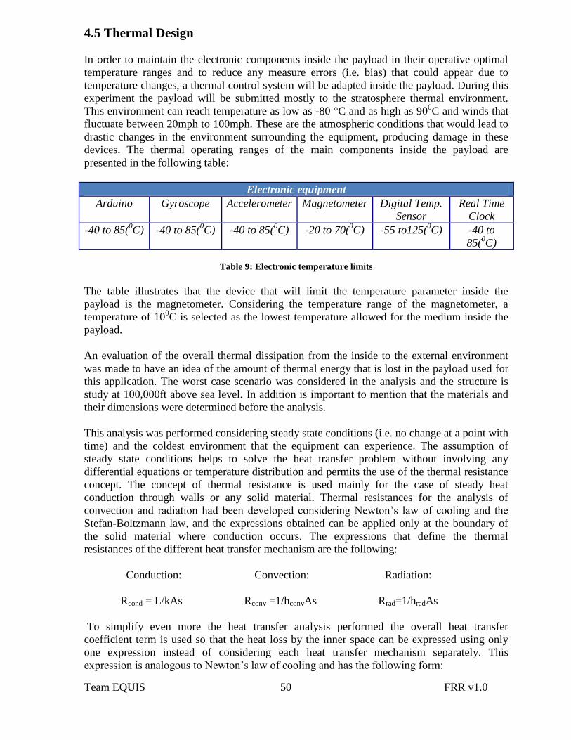
Team EQUIS 50 FRR v1.0
4.5 Thermal Design
In order to maintain the electronic components inside the payload in their operative optimal
temperature ranges and to reduce any measure errors (i.e. bias) that could appear due to
temperature changes, a thermal control system will be adapted inside the payload. During this
experiment the payload will be submitted mostly to the stratosphere thermal environment.
This environment can reach temperature as low as -80 °C and as high as 900C and winds that
fluctuate between 20mph to 100mph. These are the atmospheric conditions that would lead to
drastic changes in the environment surrounding the equipment, producing damage in these
devices. The thermal operating ranges of the main components inside the payload are
presented in the following table:
Electronic equipment
Arduino Gyroscope Accelerometer Magnetometer Digital Temp.
Sensor
Real Time
Clock
-40 to 85(0C) -40 to 85(
0C) -40 to 85(
0C) -20 to 70(
0C) -55 to125(
0C) -40 to
85(0C)
Table 9: Electronic temperature limits
The table illustrates that the device that will limit the temperature parameter inside the
payload is the magnetometer. Considering the temperature range of the magnetometer, a
temperature of 100C is selected as the lowest temperature allowed for the medium inside the
payload.
An evaluation of the overall thermal dissipation from the inside to the external environment
was made to have an idea of the amount of thermal energy that is lost in the payload used for
this application. The worst case scenario was considered in the analysis and the structure is
study at 100,000ft above sea level. In addition is important to mention that the materials and
their dimensions were determined before the analysis.
This analysis was performed considering steady state conditions (i.e. no change at a point with
time) and the coldest environment that the equipment can experience. The assumption of
steady state conditions helps to solve the heat transfer problem without involving any
differential equations or temperature distribution and permits the use of the thermal resistance
concept. The concept of thermal resistance is used mainly for the case of steady heat
conduction through walls or any solid material. Thermal resistances for the analysis of
convection and radiation had been developed considering Newton’s law of cooling and the
Stefan-Boltzmann law, and the expressions obtained can be applied only at the boundary of
the solid material where conduction occurs. The expressions that define the thermal
resistances of the different heat transfer mechanism are the following:
Conduction: Convection: Radiation:
Rcond = L/kAs Rconv =1/hconvAs Rrad=1/hradAs
To simplify even more the heat transfer analysis performed the overall heat transfer
coefficient term is used so that the heat loss by the inner space can be expressed using only
one expression instead of considering each heat transfer mechanism separately. This
expression is analogous to Newton’s law of cooling and has the following form:

Team EQUIS 51 FRR v1.0
Q=UA∆T
where:
U = overall heat transfer coefficient
UA = 1/Rtotal
Is important to mention that convection was examined in this analysis so that all the possible
heat transfer mechanism that could occurred in the stratosphere can be considered. “The
stratosphere contains very dry air which is the medium that allows the presence of convection
in that layer of the earth atmosphere” (National Center for Atmospheric Research, 2009, ¶. 4). Natural convection was considered in the payloads inside, but at the outside forced convection
is the mean of heat transfer considered. For the analysis of natural convection at the payloads
inside the following terms were determined:
β = (1/T)ideal gas
GrL=
Pr =
Nu =
For the analysis of external forced convection at the payloads outside the following terms
were determined:
Nu =
Re =
The terms used in the convection analysis are mainly used to define the convection heat
transfer coefficient h which can be determine for different cases once the Nusselt number had
been evaluated.
The radiation in this analysis is only considered in the payloads inside and this is because the
structure in this analysis is examined in the coldest environment that can occur only during
night. For the evaluation of radiation in the payload the following equation was used:
represents the variation of the
density of a fluid with temperature
at a constant pressure.
represents the ratio of the buoyancy
force to the viscous force acting on
the fluid. (Grashof number)
represents the ratio between the
velocity boundary layer and the
thermal boundary layer form in the
contact surface between a fluid and
a solid surface. (Prandtl number)
Dimensionless convection heat
transfer convection (Nusselt
number)
represents the enhancement of heat
transfer through a fluid layer as a
result of convection relative to
conduction across the same fluid
layer.
represents the ratio between the
inertial forces and the viscous
forces. Used to determine the fluid
flow regime. (Reynolds number)

Team EQUIS 52 FRR v1.0
Qrad eq = єFR4 σAeq (Ts4- Tin
4)
A summary of the analysis performed is presented in the appendix. The results obtained show
that for this application 5 W of heat are lost from the payload’s inside. This were the results
obtained from the analysis of the coldest environment that the payload can experience. The
other case that was considered was the worst warm case that the payload can experiment. The
measures considered to protect the payload for this case involve the use of reflective material
in the walls of the payload’s external structure to reflect a considerable portion of the sun rays
received and also the walls of the external structure in its inside will be polished to improve
the emissivity of the material so that the rate of heat transfer that moves from the inside to the
outside can be increased. A table that illustrates how this surface treatment can change the
emissivity of the material is the following:
Aluminum 0C Emissivity
Unoxidized 100 0.03
Commercial Sheet 100 0.09
Roughly Polished 100 0.18
Table 10: Effects of the surface treatment in the emisivity
4.6 Mechanical Design
The first step in the mechanical design was to determine which type of aluminum alloy was
the appropriate for this application. This alloy was selected considering that the structures
have to withstand thermal and mechanical loads during the various mission phases. Weight
was another important parameter considered for the material selection, since there is a
maximum value of mass that can’t be exceeded in this project (i.e. 3kg). The materials
examined are presented in the following table:
Aluminum ρ (Mg/m³) (Mpa) (Mpa) K ( /m
6066-T6 2.71 255 131 167
2014-T6 2.79 414 172 154
2014-T4 2.79 290 262 134
7075 2.8 220 150 130
1060 2.7 83 55 234 Table 11: Alloy Selection
The aluminum 6061-T6 was the alloy selected for this application because of its advantages
compared with the other materials. As can be observed from the table this material posses the
best combination of thermal and mechanical properties necessary for this application. In
addition Polystyrene Foam was the insulating material selected for this project. Polyester
foam was selected because of its low cost and low conductivity (i.e. 0.08W/mK). These
characteristics are what make this material a good option for heat transfer problems,
specifically for applications with weight limitation. The payloads geometry selected is
basically a cube; this symmetrical geometry facilitates the structural and thermal analysis of
the payload as well as the computation of any unknown dimension. The cube structure made

Team EQUIS 53 FRR v1.0
of aluminum will be form using assembling methods that basically consist of joining
aluminum square pieces using l shape brackets. This structure was selected considering the
maintenance of the structural stresses within a considerable range during the payload’s ascent
and descent.
4.6.1 External Structure
The external structure is basically a cube used to provide the first thermal and mechanical
protection to the equipment inside the payload. It’s a box built with polystyrene insulation in
its core and aluminum skin at its outside. The external aluminum structure is constituted of
four sides that are made using the aluminum alloy 6061 which is a common type of alloy used
for space applications where the weight and resistance of the materials are important factors.
The top cover of the external structure is also made from aluminum and is attached to the rest
of the structure using brackets. The bottom cover is provided by HASP personnel and is
attached to the rest of the structure using the same type of brackets used for the sides and top
parts of the payload’s structure. An illustration of the payload’s wall is provided in the
following figure:
Figure 49:Payload”s Top Cover
The previous figures is used to illustrate the basic components of the payload structure. As
can be observed from the figure the payload’s walls will be painted with a reflective color at
its outside surface and at the inside surface will be treated to increase the emissivity of the
aluminum so that the payload’s heat transfer rate from the inside can be increased. These
features will help to prevent any overheating of the internal components due to the
stratosphere’s environment. A complete illustration of the payloads external structure is
shown in the following figure:

Team EQUIS 54 FRR v1.0
Figure 50: Internal View of the External Structure
The mounting plate will be attached to the payload’s external structure using L-shape
brackets. The following figure is used to illustrate this feature.
Figure 51: External Structure Drawing
As can be observed from the previous figure four L-shape brackets will be used to secure the
payload to the mounting plate. This amount of couplers will create a strong bond between the
mounting plate and the payload’s structure, which is required for the structure, since the
payload will be exposed to a 10 g vertical and 5 g horizontal shock. An analysis was made
using two different software (i.e. Solidworks and ANSYS) to determine the stresses develop
during the payload flight whit the purpose of verifying that the structure is capable enough to
resist the stresses developed in its components during its flight. Figures that illustrate the
results obtained from these analyses are the following:
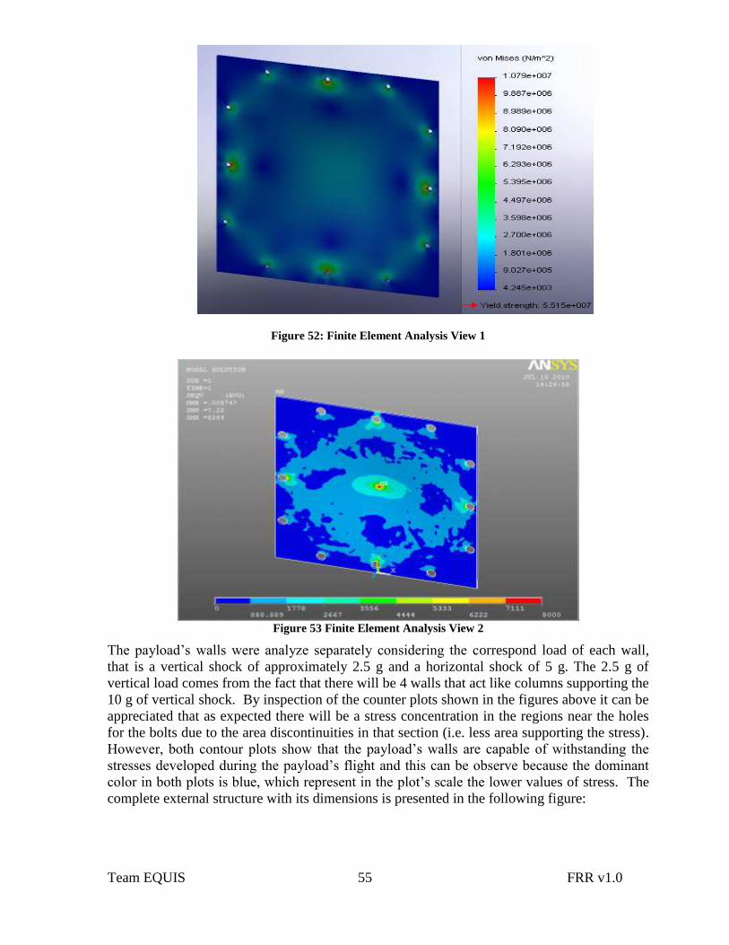
Team EQUIS 55 FRR v1.0
Figure 52: Finite Element Analysis View 1
Figure 53 Finite Element Analysis View 2
The payload’s walls were analyze separately considering the correspond load of each wall,
that is a vertical shock of approximately 2.5 g and a horizontal shock of 5 g. The 2.5 g of
vertical load comes from the fact that there will be 4 walls that act like columns supporting the
10 g of vertical shock. By inspection of the counter plots shown in the figures above it can be
appreciated that as expected there will be a stress concentration in the regions near the holes
for the bolts due to the area discontinuities in that section (i.e. less area supporting the stress).
However, both contour plots show that the payload’s walls are capable of withstanding the
stresses developed during the payload’s flight and this can be observe because the dominant
color in both plots is blue, which represent in the plot’s scale the lower values of stress. The
complete external structure with its dimensions is presented in the following figure:

Team EQUIS 56 FRR v1.0
Figure 54: Detail drawings of payload
4.6.2 Internal Structure
The internal case is used to provide thermal and structural support for the internal components
which are in this case electronic devices. The internal case is basically a box build using
polyester foam. The foam will be utilized as an insulation and also as a damper for any impact
that the electronic components could experience during the payload’s flight. The internal case
has the same geometry and building concept used in the external structure, but with a
difference in building materials and dimensions used. An example of how the payload should
look from the its top is illustrated in the following figure:
Figure 55: Top view payload structure
Insulation External
Structure
Electronic
Components L-shape
Brackets

Team EQUIS 57 FRR v1.0
Is important to mention that a set of holes will be made in the internal structure to route the
electrical cables to the payload’s inside. These cables are necessary for the electrical and data
connections. The polyester foam used for the internal case is a material commonly used for
payloads missions. The following table contain a list of important properties of the polyester
foam:
Polyester Foam Properties
Density Thermal
Conductivity
Specific Heat Young Modulus Tensile Strength
1050 kg/m3 0.08 W/(m-K) 1.3 kj/kg.k 3000 MPa 46-60MPa
Table 12 Polyester Properties
The figure # contains a complete description of the payload’s inside structure with all the
dimensions and necessary views:
Figure 56: View of punctures on structures
The internal structure will be protected by the external structure which withstand all the loads
directly and by the insulation material that enclose this part of the payload. All the important
dimensions and drawing views of the external structure are provided in the following figure:
Figure 57: Internal Structure Drawing

Team EQUIS 58 FRR v1.0
4.6.3 Mass Budget
In this project the maximum mass allowed for a small payload is 3kg. The approximate value
of the total mass of our payload is 2682.05g. This total mass was determined using values
obtained from the Solidworks (CAD software) mass properties feature and considering
approximated values for the PCBs and microcontroller (i.e. Arduino). The masses obtained
directly from the software were the insulation, the external structure and the internal structure.
The value of
the PCBs were base in past experiment of this kind. To eliminate any bias introduced by the
presumed mass values of the PCBs and to work in conservative range of values, the mass
value of the PCBs observed in previous experiment was increased from 95g to 100g for each
board. Also the mass value of the microcontroller board was approximated to 100g. The
following table is used to show the payload’s main components and their masses.
Component Mass (grams)
External Structure 950.29
Internal Structure 616.41
Insulation 815.35
Two PCB (approximately) 200
Arduino 100
Total Mass 2682.05
Table 13: Mass Budget
It can be observed considering the total mass value, that even with the increment of mass in
the PCB values we still have 317.95g that can be used for any component that is not
considered in this moment.
5.0 Payload Development Plan
Prior to the payload fabrication in the development phase various task should accomplished
such as verifying calculations, designs, prototyping and testing. This is done to resolve issues
that can only be fulfilled through testing results made to the prototype. The areas that will be
mostly focused on will be software, electrical and mechanical.
On the software, tests and measurements will be obtained to identify the size of files
developed when storing data to the SD card. It is necessary to establish the processing time of
the program which is obtained by prototyping. Verify that all interfaces, connections, and
programming will work as plan, otherwise apply the suitable contingency plan previously
develop. Simulate or develop a model to ensure that the microcontroller can communicate
through proper connections that will be used for telemetry purpose.
The electrical section will involve prototyping the signal conditional for the external
temperature sensor and the sun sensor to verify the output response and perform calibrations.
Develop the complete design of the print circuit board and develop a prototype. Perform the
prototyping and calibration for the temperature sensor. Proving that the degrees calculated
with the sun sensor data are approximately identical to the sun positioning measured.

Team EQUIS 59 FRR v1.0
Mechanical prototyping will be performed to ensure optimal quality in the payload’s structure.
Test will be performed to ensure the thermal characteristics calculated are similar to the
characteristics and behavior physically.
For the prototyping parts are necessary to be order with a degree of urgency thus requiring a
organize list of parts with sequence. The order the part must be order is:
1. Arduino
2. Magnetometer
3. Gyroscope
4. Accelerometer
5. Slot and SD Memory Card SDHC compatible
6. Payload Structure materials
More detail on order or purchase of parts can be observe in the table in section 10.1
6.0 Payload Construction Plan
When we have the component dimensions we will start sketching for a box that meets the size
and making an estimate of the weight. After the sketching we will start making possible real
size models and testing then. When we finish with the result we will make the final box and
test it with all of the components.
6.1 Hardware Fabrication and Testing
The hardware fabrication will be worked in parallel since the measurement of the payload
enclosure is known, allowing the members to start their respective sections. There will be
various tests done in the mechanical section such as thermal, impact, stress, strain and
vibration. On the electrical part there will be test in current and power dissipation, verifying
that circuits work properly. In the software development there will be a test of all sensors to
make sure it is giving and storing the proper data. The parts and components will be ordered
as soon as possible to prevent shipping delays. If a delay were to happen the team will work
on other areas accordingly until the parts are received to reduce downtime.
6.2 Integration Plan
A mechanical interface mounting plate will be provided to for the payload. The thickness of
the mechanical interface mounting plate is ¼” PVC. The payload will be enough attached to
the mounting plate that can handle 10g vertical and 5g horizontal shock. The mounting plate
includes an EDAC 516-020 connector for power. The EDAC connector will be the power
interface between the payload and the HASP platform.

Team EQUIS 60 FRR v1.0
Figure 58: EDAC pin layout
The EDAC 516 for HASP has twenty pins as shows Figure 54. The pins function and the
color code for the wires of the EDAC 516 are explained in the Table 13.
Function EDAC Pins Wire Color
30VDC A, B, C, D White with red stripe
Power Ground W, T, U, X White with black stripe
Analog 1 K Blue
Analog 2 M Red
Signal Return L, R Black
Discrete 1 F Brown
Discrete 2 N Green
Discrete 3 H Red with white stripe
Discrete 4 P Black with white stripe Table 14: EDAC 516 pins function and color code
As shows Table 1, the +30VDC delivered power from the HASP platform can be received
through the pin A, B, C and D of the EDAC 516 interface and the ground can be provided by
the pins W, T, U and X.
6.3 Software Implementation and Verification
The first step is to design the program to meet the Pro 328 needs and run it for testing
purposes. The sensor code will be develop separately and tested to verify proper functionality,
then the code structure will be develop to join all the different sensor code and tests with the
complete code. If errors and problems appear they will be verified for electrical errors, if no
electrical errors code will be corrected.
This phase will be executed as follow:
Determine the required bytes
Flowchart analysis
Sensor calibration
Display sensor data during testing
Verify Arduino’s processing time

Team EQUIS 61 FRR v1.0
6.4 Flight Certification Testing
To certify that the ADS payload is ready for flight it is necessary to reproduce test with
conditions that could occur during flight, such as pressure, temperature changes and impact
test when the payload is lands. By doing this prevents possible failures that can occur, such
electrical failure due to any of the different conditions just mentioned.
The following tests were concluded:
Vacuum Test
The testing will be done by:
Styrofoam to hold the sensors in place
Full system test
o Payload shock testing
o Payload temperature
o Payload vacuum testing
Electrical system testing
o PCB board continuity test
o Cable connection testing
o Electronic components test (IC- integrated circuit testing)
6.4.1 System Testing Procedures
Vacuum Test
The vacuum test was performed with in a vacuum chamber with the capability of (35psi) in
the physics and astronomy department as shown in Figure 59.
Figure 59 Psi Vacuum chamber
The payload was placed in the chamber, sealed and the test was initiated. The test was
fulfilled by raising the pressure by a factor of 10 up to 30psi, for each pressure the payload
was left for 10 min as the pressure raised and as it went down to cero.
Temperature Test
This test requires placing the payload in four different temperatures stages, starting from the
highest to the lowest temperature and then at the same rate reducing the temperature to the
lowest. First it was placed outside at ambient temperature for 10min then it was placed at
room temperature 25oC, then it was place in a freezer for 10mins and then it will be place in a

Team EQUIS 62 FRR v1.0
box with dry ice. Then the same procedure will be performed until the temperature is finally
ambient temperature. Figure 60 shows the box where it was placed with dry ice.
Figure 60 Chamber where temperature test was taken
Shock test
The shock test consist of dropping the payload while fully functional and talking data, from a
height of approximately 10 feet as shown in Figure 61.
Figure 61: Shock Test

Team EQUIS 63 FRR v1.0
6.4.2 System Testing Results
Vacuum Test
During the time payload was tested it operated correctly during the complete test, the values
obtained will be shown in the Table in Appendix D. The complete test the payload
successfully kept gathering data and function properly... The values of the sensor remained
throughout the test the same…. In the result analysis after the calibration the data will be
plotted and explained in detail. It is important to identify that the output is raw data, later it
will be converted to significant values for each sensor.
Temperature Test
Throughout the temperature test the payload was being exposed to different temperatures for
a determined period of time. The results of the data will be in Appendix D, the results should
show that the all the components function properly during the complete test. The data that will
have change will be the temperature; this data will be plotted as a temperature vs time
analysis. Also plots of sensor data vs. temperature will be completed.
Shock Test
For the shock test the result showed that the payload is capable of a withstanding the impact
while taking data from the sensor without failure. In Appendix D the table shown has the
values obtained during this test. By observing the values it can be observed the electrical
components and the structure is capable of passing the impact test.
7.0 Mission Operations
Equipment final checkup
Complete system integration
Place the equipment on the launch site
Ground platform tracking
Data analysis
o Data retrieval
o Data conversion
o Data plots
o Plot analysis
7.1 Pre-Launch Requirements and Operations
A successful flight testing in simulated environment (similar to that were the payload is going
to be, such as vacuum and thermal testing) will be done to make sure that the sensors are
working as expected. The Arduino also needs to boot up and run the pre-flight software to
ensure the memory will be clean, in other words with 0 data in the SD card.
7.1.1 Calibrations
Proper sensor calibration, with the recommended procedure suggested by the manufacturer,
needs to be done to all of the sensors in the ADS payload.

Team EQUIS 64 FRR v1.0
Magnetometer Calibration
Calibration of the MicroMag3 is necessary to comprehend the raw data obtained by the
attitude determination system, to obtain orientation. Calibration will be made by using a
Helmholtz Coil shown in Figure 62, this payload is centered with two large coils (Helmholtz
coils) to receive a uniform magnetic field.
Figure 62 Helmholtz coils
By placing the ADS payload in the center of the coil it is possible to compare the values of the
magnetometer with the calculated values of the field in the Helmholtz. The field in the
Helmholtz is calculated with the following equation:
Where
B= Magnetic filed in Teslas
µ0= Magnetic permeability of vacuum in N/A2
N= number of turns
I = current in Amperes
R= radius of the coil in meters
The Helmholtz has an N of 70 turns and a radius for the coils of 26.4cm; with the power
supply it is possible to find the magnetic field by knowing the current. The following equation
is a simplified form of the previous equation to obtain the field magnitude with a controlled
current.
This test was done with the MM3 without ADS payload, the result obtained when the current
was cero was approximately 400counts and with a current of 1A the output was approx. 8400
on the positive x-axis similar, the count of the magnetic field was 8000counts. By applying
the following we obtained a gain of 33.58counts/µT, this values is similar to the gain on the
datasheet of 31.24counts/ µT.
MM3

Team EQUIS 65 FRR v1.0
Notice on Table 14 the x-axis has values much larger than the other axis, because this is the
concerning one at this instant.
X Y Z
8407 357 489
Table 15 Example of raw data from the MM3
To convert the raw data all that needs to be done is to multiply the counts of the axis and
multiply it by the gain calculated for that axis. For the each axis the same procedure must be
done.
The calibration values based on the data obtained at each axis both on the positive side and
negative side can be obtained with the equations in Table 15.
Xoffset= Xmax+ Xmin
Calculates the Offset Yoffset= Ymax+ Ymin
Zoffset= Zmax+ Zmin
Xrange= Xmax- Xmin
Calculates the Range Yrange= Ymax- Ymin
Zrange= Zmax- Zmin Table 16: Calibration values
Where
Xmax & Xmin are the maximum and minimum values obtained in the X-axis
Ymax & Ymin are the maximum and minimum values obtained in the Y-axis
Zmax & Zmin are the maximum and minimum values obtained in the X-axis
To correct the offset the following equations in Table 16 must be applied to the values of the
magnetometer.
Xvalue = Xraw - XOffset
Yvalue = Yraw - YOffset
Zvalue = Zraw - ZOffset Table 17: Equations to correct offset
Note that if the values of the Xrange are greater than the Y range it is necessary to match the
gain by using the following equation:
Since tan-1
results is only in the range of 0 to 90 it is important to note the sign of the X and Y
to determine the proper quadrant and to add the correct padding to determine it direction, this
is assisted by using the values in Table 17.
X value Y value Formula Quadrant
D= Ө +X +Y 0-90
D=180 - Ө -X +Y 90-180

Team EQUIS 66 FRR v1.0
D=180+Ө -X -Y 181-270
D=360 - Ө +X -Y 271-359 Table 18: Quadrant determination
To obtain the calibration equations the values obtained from the magnetometer are plotted and
compared with the known magnetic field of the Helmholtz as in Figure 63.
Figure 63: Helmholtz coil (X) vs MM3 (Y)
With figure # it can be observe the a linear fit for the set data will allow a calibration equation
which is
F=0.9624(DCounts) – 25.40
Where
F = Helmholtz field
DC= Digital Counts (raw data)
Digital Temperature Sensor (DS18B20)
As mentioned in Section 3.4.1 Technical Background and 4.3.1 Sensors Subsystem, the
internal temperature of the payload will be gathered using a DS18B20 Digital Temperature
Sensor. The DS18B20 will be calibrated by placing this sensor with a calibrated temperature
sensor
(HOBO) inside the payload and exposing the payload to a temperature profile. These
measurements will be stored during the temperature profile to develop a graph with both
measures and compare the readings of the DS18B20 with the reading of the calibrated
temperature sensor. A plot can be generated using both measurements to obtain an equation to
adjust the output of the DS18B20 and calibrate the data obtained from this sensor; as a result,
the data of the DS18B20 will be calibrated in the post flight analysis phase using the gathered
equation to realize some adjustments to the output of the DS18B20.
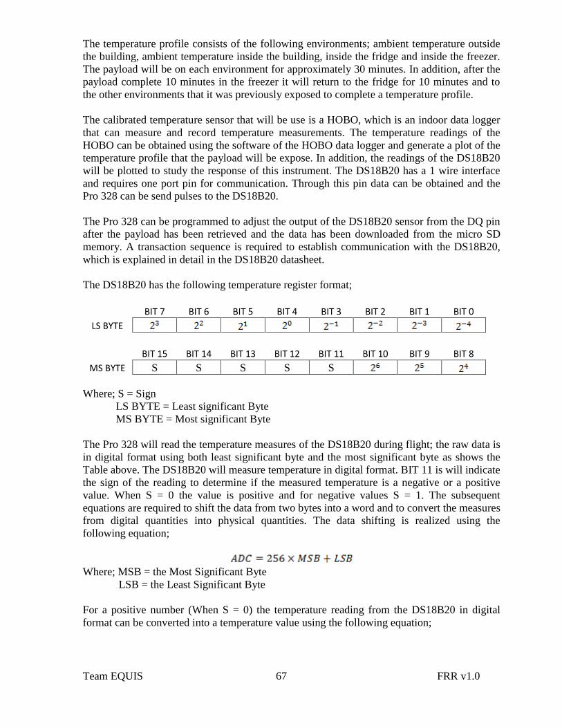
Team EQUIS 67 FRR v1.0
The temperature profile consists of the following environments; ambient temperature outside
the building, ambient temperature inside the building, inside the fridge and inside the freezer.
The payload will be on each environment for approximately 30 minutes. In addition, after the
payload complete 10 minutes in the freezer it will return to the fridge for 10 minutes and to
the other environments that it was previously exposed to complete a temperature profile.
The calibrated temperature sensor that will be use is a HOBO, which is an indoor data logger
that can measure and record temperature measurements. The temperature readings of the
HOBO can be obtained using the software of the HOBO data logger and generate a plot of the
temperature profile that the payload will be expose. In addition, the readings of the DS18B20
will be plotted to study the response of this instrument. The DS18B20 has a 1 wire interface
and requires one port pin for communication. Through this pin data can be obtained and the
Pro 328 can be send pulses to the DS18B20.
The Pro 328 can be programmed to adjust the output of the DS18B20 sensor from the DQ pin
after the payload has been retrieved and the data has been downloaded from the micro SD
memory. A transaction sequence is required to establish communication with the DS18B20,
which is explained in detail in the DS18B20 datasheet.
The DS18B20 has the following temperature register format;
BIT 7 BIT 6 BIT 5 BIT 4 BIT 3 BIT 2 BIT 1 BIT 0
LS BYTE
BIT 15 BIT 14 BIT 13 BIT 12 BIT 11 BIT 10 BIT 9 BIT 8
MS BYTE S S S S S
Where; S = Sign
LS BYTE = Least significant Byte
MS BYTE = Most significant Byte
The Pro 328 will read the temperature measures of the DS18B20 during flight; the raw data is
in digital format using both least significant byte and the most significant byte as shows the
Table above. The DS18B20 will measure temperature in digital format. BIT 11 is will indicate
the sign of the reading to determine if the measured temperature is a negative or a positive
value. When S = 0 the value is positive and for negative values S = 1. The subsequent
equations are required to shift the data from two bytes into a word and to convert the measures
from digital quantities into physical quantities. The data shifting is realized using the
following equation;
Where; MSB = the Most Significant Byte
LSB = the Least Significant Byte
For a positive number (When S = 0) the temperature reading from the DS18B20 in digital
format can be converted into a temperature value using the following equation;

Team EQUIS 68 FRR v1.0
For a negative number (When S = 1) the temperature reading from the DS18B20 in digital
format can be converted into a temperature value using the following equation;
The temperature measurements are placed from BIT 4 to BIT 11; however, the code for the
DS18B20 will shift 16 bit number, so that the measure will start at BIT 0 instead of BIT 4; as
a result, the measurement value will be from BIT 0 to BIT 7.
Table 19: DS18B20 versus HOBO temperature measures
The Table 18 shows simulated measurements obtained from both; the DS18B20 temperature
sensor and the HOBO during the temperature profile. Both sensors were inside the payload
during the temperature profile. For the temperature profile the payload remained on each of
the five different environments; ambient temperature outside the building, ambient
temperature inside the building, the fridge, the freezer and the dry ice for approximately 10
minutes.
HOBO data (°C) DS18B20 data (°C)
30 28
20 18
10 7
5 4
-10 -12
5 4
10 7
20 18
30 28

Team EQUIS 69 FRR v1.0
Figure 64: Linear Fit
Figure 64 shows the temperature measurements from both sensors; the DS18B20 and the
HOBO temperature sensor. This graph was developed using the Graphical Analysis 3.2
software. Note that there is a small difference between the temperature measures of the
DS18B20 and the HOBO measures; therefore, an equation is required to make fine
adjustments to the change the output values from the sensor into a calibrated response.
The subsequent equation is required to convert the measures from digital quantities into
physical quantities. This equation was obtained using the data and the Graphical Analysis
software;
Where; The temperature measured by the DS18B20
The raw data of the DS18B20
The gain
The Offset
Accelerometer Calibration
The SCA3000 Three axis accelerometer sensor will have an output response when a
capacitance change occurs due to acceleration. Once the accelerometer sensor arrives the
prototype for the accelerometer sensor will be implemented to perform the required tests. The
accelerometer prototype will be exposed to at least three different acceleration positions on
each one of its axes to determine the output response of the sensor at that particular
acceleration. The next step is to assign a digital value to each one of the selected outputs
response of the accelerometer to obtain a linear equation that will relate the outputs with the
digital values.
Gyroscope Calibration

Team EQUIS 70 FRR v1.0
The ITG-3200 Three axis gyroscope sensor will measure the rate of rotation; as a result, the
sensor will have an output response when sense a change in rotation in each one of the axis.
Each axis will be rotated at approximately the same rate of rotation to have a similar
calibration for each axis. After rotating each axis at a particular rate of rotation and obtain the
output response, a linear equation can be created to relate the digital values with the
gyroscope output response.
7.1.2 Pre-Launch Checklist
Make sure all the instruments are working properly
Realize a final check of the prototype comparing it with the schematics and the
simulations
Revise the list of test, such as thermal and vacuum test to ensure that all the testing has
been accomplish
Run all the program and make sure are working properly
Bring all the necessary equipment for any emergency
7.2 Flight Requirements, Operations and Recovery
The payload will ascend up to an altitude of 120,000 ft for approximately 2 hours and remain
there for 16 hours total. The payload and components will have to support temperature
conditions of an expected -40 degree of temperature. The system needs the sensors to read all
the time to get all the data during the flight. The batteries must be able to support the flight
with the minimum required power. If the batteries are not in the minimum required power
then the circuit would be in equilibrium with the sensor voltage required for them to work.
The experiment needs a GPS or any radiofrequency tracking device of high power so we can
track the altitude in which the payload is located and to track the retrieval of the payload in
the landing site.
7.3 Data Acquisition and Analysis Plan
The Arduino Pro requires an SD card memory module for the storage of the data during the
flight then we going to download the data using an Arduino Pro and a serial/USB cable in
which is going to be connected from the payload to the computer software but to process the
receiving data we need to convert the measurement in ADC counts requiring some equations
for the convection of ADC to physical values then we analyze the data of the atmosphere and
flight of the payload.
7.3.1 Ground Software
The ground software requires the following components; a microcontroller (Atmega 328), a
serial/USB cable, the code to download the data and a computer to process the information
and download the data from the payload. Graphical analysis 3.2 for plot the data will also be
needed.
7.3.2 Data Analysis Plan

Team EQUIS 71 FRR v1.0
The first step on the ground station after the land will be to use the post flight program to take
the data from the payload. The software will be prepared using the Arduino IDE. We will
implement some software for the calibration of the sensors. The data will be store using ADC
counts to represent the measurements from the sensors. In the process of receiving the data,
the ADC will convert the measurements into ADC counts that will be stored in the SD card.
This requires some equations to convert from ADC counts to physical values. Some
uncertainties during the launch are expected as well as in the balloon cut off and in the
landing. Expecting those irregularities, make some extra calibrations looking for the most
precise measurements.
8.0 Project Management
To ensure documentation version control a single team member (A.M. Espinal Mena) will be
the team member that will have the latest version of all the documentation. It has been agreed
that when a team member do a modification in the PDR, CDR and FRR they have to send an
e-mail of the modification to this team member, so she can add it to the proper document and
send a notification to the rest of the team so they can now which parts has been updated. In
addition to the days of class regular meetings in the week to monitor the progress of the
project will be scheduled.
8.1 Organization and Responsibilities
The EQUIS Team consists of three students of the Inter American University of Puerto Rico,
Bayamón Campus. The responsibilities of these students are to work on the following part of
their experiment; the electrical/mechanical designs, prototype development, fabrication,
integration and testing of the payload that will be launch with a balloon. The name of the
students of the EQUIS Team and their tasks are as follows:
A. M. Espinal Mena, [email protected], Electrical Design, Prototype and
Calibration
E. M. Portilla Matías, [email protected], Software Design and Implementation
F. O. Rivera Vélez, [email protected], Mechanical and Thermal Design
J. I. Espinosa Acevedo, [email protected], Prototype and Calibrstion, Risks
and Management plan
8.2 Configuration Management Plan
Every time a design is made we consult with the team member so we can make a decision of
the design and to analyze de advantage and disadvantage of the design before getting
approved.
8.3 Interface Control
Interface control allows us to maintain a constant monitoring of the Flight Readiness Review
(FRR) document at all times. It was established in a group meeting to assign one person in
charge of the FRR, this person will be in charge of constantly adding new information to the
document and uploading its final version, this way every member will allow access to the file.
Also an online group section was established where all document will be uploaded. It was
notified to the members that every time a document is uploaded or any change will be made to

Team EQUIS 72 FRR v1.0
notify Ana Espinal through a call, which is the person in charge of the FRR, doing so she will
be aware of any modifications. Finally a group meeting will be held to verified the complete
document and ensure it is the final version before submitting.
9.0 Master Schedule
We establish to divide the tasks into different member of the team but some task will be in
parallel with the other task, because this will makes us to meet the experiment goal. The
amount of days assigned to each task is shown in the Figure 62. Following the work
breakdown schedule is essential to realize the mission of this experiment.
9.1 Work Breakdown Structure (WBS)
Figure 65: WBS- Work Breakdown Schedule
Figure 65 shows the WBS of the EQUIS team to complete the EQUIS payload and
instruments on time.
9.2 Staffing Plan
A. M. Espinal Mena- Electrical design, Prototype and Calibration
E. M. Portilla Matías- Software Design and Implementation
F. O. Rivera Vélez- Mechanical and Thermal Design
J. I. Espinosa Acevedo- Prototype and Calibrstion, Risks and Management plan
Advisor: Dr. H. B. VO/ E. G. Delgado

Team EQUIS 73 FRR v1.0
9.3 Timeline and Milestones
The PDR, CDR and FRR documents have to be submitted by the following deadlines:
PDR- Preliminary Design Review due March 5, 2010
PDR Revision- Preliminary Design Review Revision due April 12, 2010
PDR Defense- Preliminary Design Review Defense June 4, 2010
CDR- Critical Design Review due July 1, 2010
FRR- Flight Readiness Review due July 23, 2010
10.0 Master Budget
The maximum capital cost budget required for this project is $5,000. It is also required to
have a reserve contingency fund of 10%, which is $500 in this case; therefore, the capital cost
budget is $4,500.
10.1 Expenditure Plan
Integrating the instruments for the ADS experiment requires several components. Table 13
shows the list of electronic components necessary to integrate the instruments, their price and
delivery status.
Lead time Sensors Part Number
Sales Company
Quantity Status Price ($)
1 Three Axis Accelerometer
SCA3000 Sparkfun 2 - $89.98
($44.99
each)
1 Three Axis Gyroscope
ITG-3200 Sparkfun 2 - $99.90
($49.95
each)
1 Three Axis Magnetometer
Micromag3 Sparkfun 2 - $119.90
($59.95
each)
1 Digital Temperature Sensor
DS18B20 Sparkfun 2 - $8.50
($4.25each)
1 Level Shift Converter
8745 Sparkfun 10 - $19.50
($1.95 each)
1 San Disk 4 GB SDSDB-
004GA14F
Amazon 2 - $17.98 ($8.99)
1 Arduino Pro DEV-09221 Sparkfun 2 - $39.90 ($19.95 each)
1 microSD transflash
BOB-00544 Sparkfun 2 - $29.90 ($14.95 each)
1 Material for housing - $500

Team EQUIS 74 FRR v1.0
11.0 Risk Management and Contingency
Risk Type Risk
Assessment of Risk Risk Control
Measures Impact Severity Likelihood Probability
Detention Difficulty
Electrical
Exceed component’s temperature
HIGH HIGH MEDIUM Provide a
heating system
Faulty connection
between cables HIGH HIGH MEDIUM
Ensure connections
and strap cable to prevent movement
Short circuit HIGH MEDIUM MEDIUM Review the PCB
population process
SD card failure HIGH LOW MEDIUM Transmit through
Telemetry
Mechanical
Temperature Leakage into
payload HIGH MEDIUM MEDIUM
Pressure and temperature
testing
Structure Failure HIGH LOW MEDIUM
Minimize apertures, use alloy 2014 and
mono-block design
Loosening of nuts and bolts
due to vibration MEDIUM LOW LOW
Use pressure bolts
Fall into wet terrain
HIGH MEDIUM LOW Ensure proper
sealing of Payload
Software
Data Corruption HIGH HIGH HIGH Store Data in SD
memory card
Loss of Data due to
Overwriting HIGH HIGH MEDIUM
Divide SD in sectors of 512bytes
Improper Logic Programming
HIGH MEDIUM HIGH Test program before flight
1 Extra PCB board - $300
1 Real Time Clock DS1306 Maxim 2 - $12.72
($6.36 each)
-- Total Cost: - $1364.18
Table 20: Materials Acquirement & Costs

Team EQUIS 75 FRR v1.0
Insufficient memory storage
HIGH HIGH LOW Obtain memory
card with greater storage
Scheduling
Not meeting FRR deadline
HIGH MEDIUM MEDIUM
Getting more hours of work and more days
in the lab
Errors in FRR HIGH MEDIUM MEDIUM Review
document various time
Table 21: Risk Management & Contingency
Through a risk management it is possible to reduce the likelihood of unexpected events. By
having a contingency plan it is possible to reduce costs and severity of a risk. This is done by
identifying, assessing and developing a strategy to response for each risk, while monitoring
for additional risks as shown in Figure 66. Table 14shows the potential risks that the EQUIS
experiment may encounter and the contingency plan that the ADS team has for each of these
risks. As illustrated in the Table 14, the potential risks have several categories. It is important
to keep constant cycle of risk management in order to control possible variables that may
affect project performance.
Figure 66: Risk Management Cycle

Team EQUIS 76 FRR v1.0
12.0 Glossary
CDR Critical Design Review
FRR Flight Readiness Review
PDR Preliminary Design Review
TBD To be determined
TBS To be supplied
WBS Work breakdown structure
HASP High Altitude Student Platform
ITS Internal Temperature Sensor
ADS Attitude Determination System
EQUIS Experiment with Quality United In Science
NEU North-East-Up
MRI Magnetic Resonance Imaging
GPS Global Positioning Satellite
SD Secure Digital
USB Universal Serial Bus
EEPROM Electrically Erasable Programmable Read-Only Memory
ADC Analog to Digital Converter
FET Field Effect Transistor
IC Integrated Circuits
PCB Printed Circuit Board
LSB Least significant byte
MSB Most significant byte

Team EQUIS 77 FRR v1.0
Appendix
Appendix A
I. Data.
Tout = -800C Qemt eq = 1W (computed)
Tin = 00C (design parameter) kalm = 134W/m
0C
kins = 0.12 W/m0C Lalm = 0.0032m
Lins = 0.005m σ = 5.67X10⁻⁸W/m2K
4 (Stefan-Boltzmann const.)
єFR4 = 0.8 єAlm = 0.07 (rough surface)
ѵair@100000ft = 8.012X10 – 4 m2/s Vmean@100000ft = 26.82m/s
ρair@100000ft = 1.841X10⁻² kg/m3 μair@100000ft = 1.475X10⁻⁵ kg/m s
II. Find
Qloss = ?
III . Diagrams
Figure 67: Heat Loss Analysis

Team EQUIS 78 FRR v1.0
IV. Analysis
Heat loss:
Qloss =UA∆T ∆T= (Tin – Tout), UA= , Rtotal = Req1+RA1,1+ Rins+RAl2+Req2
Thermal Resistances:
Req2 = hcomb = hrad,in + hconv,in hconv,in = ? ; hrad,in = ?
Equipment power radiation:
Qrad eq = єFR4 σAeq (Ts4- Tin
4) Ts =Tin +
Ts=450K=1820C; Aeq=0.01198m
2
Qrad eq = hradAeq (Ts- Tin ) hrad,in = = 0.27W/m
2 0C
Internal Convection:
NuL = = ; L =0.1m ;
s=0.06m (distance between boards)
Ra,s = ; B = ; g@100,000ft=9.715m/s2
Tf = = 150C = 288K ; B = 0.003472/K; Pr=0.7362; k=0.02364W/m
0C
Ra,s = 530.19 RaL= Ra,s (L3/s
3) = 306.82
NuL =1.79 = hconv=0.71W/m0C hcomb,in ≈ 1W/m
2 0C
Therefore:
Req2 = 83.5 0C/W
Req1 = hcomb = hrad,out + hconv,out hrad,out = ? hconv,out = ?
Qrad out = єAlm σAs (Ts4- Tout
4) = 84.8mW, hrad,out = = 0.15W/m
2 0C
-0.5
Ideal
gas

Team EQUIS 79 FRR v1.0
For external convection:
Walls modeled as:
Figure 68: External Convention
Re = where Lc = L Re = 4686 = 4.69X10³
Recr =5X10
5 Re < Recr (laminar flow regime)
Therefore:
Nu = = 0.664 ReL0.5
Pr1/3
With interpolation a Pr = 0.7394 is obtained
Nu = 41.1 h = 5.51 W/m2 0
C hcomb = 5.66 W/m2 0
C Req1 = = 9.710C/W
Rcond, eq = Alm,out + ins + Alm,in = 3.31 0C/W
Rtotal = Req1+ Rcond, eq +Req2 =96.52 0C/W UA= = 0.0104W/
0C
Qloss for each side is
Qloss =UA∆T= 0.78W (considering the six sides) Qloss,max =6 Qloss W
Vmean
Tout Ts
L`

Team EQUIS 80 FRR v1.0
Appendix B
Sensors Subsystem Schematic and PCB design
Schematic design

Team EQUIS 81 FRR v1.0
PCB design

Team EQUIS 82 FRR v1.0
Appendix C
RTC (DS1306) pseudo code
spi_transfer(data)
SET SPDR to data
WHILE (NOT (SPDR AND (SET SPIF to 1))) DO
ENDWHILE
RETURN with SPDR
initializeRTC()
SET SPCR to enable SPI, master or slave, and clock frequency
SET slave select line to HIGH
input rtcRegister, setRtc_num
CALL spi_transfer with rtcRegister
CALL spi_transfer with setRtc_num
SET slave select line to LOW
receiveTimeStamp()
input time, rtcRegister, zero
SET zero to 0
SET SPCR to enable SPI, master or slave, and clock frequency
SET slave select line to HIGH
CALL spi_transfer with rtcRegister
CALL spi_transfer with zero RETURNING time
SAVE time to SD card
SET slave select line to LOW

Team EQUIS 83 FRR v1.0
Magnetometer (MicroMag3) pseudo code
receiveMicroMagData()
FOR axis = 0 TO 2
SET SPCR to 0
SET slave select line to LOW
SET reset line to LOW
SET reset line to HIGH
SET reset line to LOW
FOR bits = 0 TO 5
IF bits == 1 OR bits == 2 THEN
SET mosi line to HIGH
ELSE
SET mosi line to LOW
ENDIF
SET sclk line to HIGH
SET sclk line to LOW
ENDFOR
IF axis == 0 THEN
SET mosi line to LOW
SET sclk line to HIGH
SET sclk line to LOW
SET mosi line to HIGH
SET sclk line to HIGH
SET sclk line to LOW
ELSE IF axis == 1 THEN
SET mosi line to HIGH
SET sclk line to HIGH
SET sclk line to LOW
SET mosi line to LOW
SET sclk line to HIGH
SET sclk line to LOW
ELSE
SET mosi line to HIGH
SET sclk line to HIGH
SET sclk line to LOW
SET mosi line to HIGH
SET sclk line to HIGH
SET sclk line to LOW
ENDIF
WHILE data ready line == low DO
ENDWHILE
input firstBit
SET sclk line to HIGH
READ miso line RETURNING firstBit
SET sclk line to LOW
input totalBits
SET totalBits to 0
FOR bits = 14 TO 0

Team EQUIS 84 FRR v1.0
SET sclk line to HIGH
input remainingBits
READ miso line RETURNING remainigBits
SET sclk line to LOW
COMPUTE remainingBits as remainingBits << bits
COMPUTE totalBits as totalBits | remainingBits SET sclk line to LOW
ENDFOR
SET slave select line to HIGH
IF firstBit == 1 THEN
COMPUTE totalBits as totalBits - 32768
ENDIF
SET SPCR to enable SPI, master or slave, and clock frequency
SAVE totalBits to SD card
ENDFOR

Team EQUIS 85 FRR v1.0
Accelerometer (SCA3000-D01) pseudo code
spi_transfer(data)
SET SPDR to data
WHILE (NOT (SPDR AND (SET SPIF to 1))) DO
ENDWHILE
RETURN with SPDR
receiveAcceData()
input data, rtcRegister,msb, lsb
COMPUTE rtcRegister as rtcRegister << 2
SET SPCR to enable SPI, master or slave, and clock frequency
SET slave select line to LOW
CALL spi_transfer with rtcRegister
CALL spi_transfer with 0 RETURNING msb
CALL spi_transfer with 0 RETURNING lsb
COMPUTE data as (msb << 8) | (lsb & 0xf8) / 8
SAVE data to SD card
SET slave select line to HIGH

Team EQUIS 86 FRR v1.0
SD card pseudo code
createFile()
input fileName, counter
SET fileName[] as "EQUIS000.CSV"
FOR number to 1000
COMPUTE fileName[5] as number / 100 + '0'
IF counter >= 100 THEN
SET counter as 0
ENDIF
IF number >= 100 THEN
COMPUTE fileName[6] as counter / 10 + '0'
INCREMENT counter
ENDIF
IF number < 100 THEN
COMPUTE fileName [6] as number / 10 + '0'
ENDIF
COMPUTE fileName[7] as number % 10 + '0'
IF fileName == false THEN
BREAK
ENDIF
ENDFOR
WRITE to fileName ",header"
saveData()
input data
CALL sensorFunction returning data
WRITE to fileName ","
WRITE to fileName data

Team EQUIS 87 FRR v1.0
Pre-flight software: /****************************
*
*
* Pre-flight
* EQUIS software
*
*****************************/
/////////////PINS//////////////
#define MISO 12
#define MOSI 11
#define SCK 13
#define RTCPIN 8
/////////////Variables/////////
byte secs;
byte mins;
byte hrs;
byte date;
byte day;
byte month;
byte year;
byte clr = 0; // used to clear data
char spi_transfer(volatile char data)
SPDR = data; // SPDR = Atmega's SPI data register
/********************************
* SPIF is bit 7 of the SPSR
* When a serial transfer is complete
* the SPIF flag is set
**********************************/
// SPSR = Atmega's SPI status register, SPIF = SPI interrupt flag
while (!(SPSR & (1 << SPIF)))
// wait until transmission is complete
;
/************************************
* SPDR is used for data transfer
* between the register file
* and the SPI shift register
************************************/
return SPDR; // return SPI data register
void set_RTC(byte register_num, byte time)
//SPCR = 0;
register_num |= 128;
/**************************************
* RTC DS1306
* SPI protocol
* sampled falling edge
* SPCR = Atmega's SPI control register
***************************************/
// SPE = enable SPI
// MSTR = sets arduino in master mode

Team EQUIS 88 FRR v1.0
// SPI mode 1
SPCR = (1 << SPE) | (1 << MSTR) | (1 << CPHA);
clr = SPCR; // clear data from past runs
clr = SPDR; // clear data from past runs
digitalWrite(RTCPIN, HIGH); // (slave) select rtc
spi_transfer(register_num); // transfer register
spi_transfer(time); // transfer data to set time
digitalWrite(RTCPIN, LOW); // (slave) deselect rtc
Serial.println("Done");
byte get_RTC(byte register_num)
//SPCR = 0;
register_num &= 127;
/**************************************
* RTC DS1306
* SPI protocol
* sampled falling edge
* SPCR = Atmega's SPI control register
***************************************/
byte temp; // temporary variable
// SPE = enable SPI
// MSTR = sets arduino in master mode
// CPHA = clock phase, sample data = falling or rising
// SPI mode 1
SPCR = (1 << SPE) | (1 << MSTR) | (1 << CPHA);
clr = SPCR; // clear data from past runs
clr = SPDR; // clear data from past runs
digitalWrite(RTCPIN, HIGH); // (slave) select rtc
spi_transfer(register_num); // transfer register
temp = spi_transfer(0); // transfer zero to receive data from
register
digitalWrite(RTCPIN, LOW); // (slave) deselect rtc
return temp;
void setup()
Serial.begin(9600); // set baud rate
pinMode(MOSI, OUTPUT);
pinMode(MISO, INPUT);
pinMode(RTCPIN, OUTPUT);
pinMode(SCK, OUTPUT);
pinMode(9, OUTPUT); // magnetometer
pinMode(7, OUTPUT); // accelerometer
pinMode(10, OUTPUT); // SPI sd card
pinMode(2, OUTPUT); // magnetometer reset
digitalWrite(RTCPIN, LOW); // use RTC, active-high
digitalWrite(10, HIGH); // SPI, active-low
digitalWrite(9, HIGH); // disable

Team EQUIS 89 FRR v1.0
digitalWrite(7, HIGH); // disable
/**************************
* clear the control register
* before any write
* write protect is in the 6th
* bit of the control register
*****************************/
set_RTC(0x8F, 0x04); // set RTC control register to 0
byte temp = get_RTC(0x0F);
Serial.print("ControlReg: "); Serial.println(temp, HEX);
set_RTC(0x80, 0x00); // set seconds write register to 0
set_RTC(0x81, 0x40); // set the minutes to 40min
set_RTC(0x82, 0x23); // set hours to 11pm to 24 hr = 23
set_RTC(0x83, 0x01); // (monday = 1, tuesday = 2, etc)
set_RTC(0x84, 0x19); // set date to the 19th
set_RTC(0x85, 0x07); // month
set_RTC(0x86, 0x10); // year 00-99
void loop()
month = get_RTC(0x05); // get month
year = get_RTC(0x06); // get year
day = get_RTC(0x03); // get day
date = get_RTC(0x04); // get date
hrs = get_RTC(0x02); // get hours
mins = get_RTC(0x01); // get minutes
secs = get_RTC(0x00); // get seconds
// Display output
switch (day)
case 1:
Serial.println("Monday");
break;
case 2:
Serial.println("Tuesday");
break;
case 3:
Serial.println("Wednesday");
break;
case 4:
Serial.println("Thursday");
break;
case 5:
Serial.println("Friday");
break;
case 6:
Serial.println("Saturday");
break;
case 7:
Serial.println("Sunday");
break;
default:
Serial.println("Error");
break;

Team EQUIS 90 FRR v1.0
Serial.print("Mn/Dd/Yr: ");
Serial.print(month, HEX); Serial.print("/");
Serial.print(date, HEX); Serial.print("/");
Serial.print("20"); Serial.println(year, HEX);
Serial.print("Hr:Mm:Ss = ");
Serial.print(hrs, HEX); Serial.print(":");
Serial.print(mins, HEX); Serial.print(":");
Serial.println(secs, HEX);
delay(1000);

Team EQUIS 91 FRR v1.0
During flight software: /***************************************
*
*
* EQUIS Software
*
*
****************************************/
//////////header files/////////////
#include <SdFat.h> // SDFat lib
#include <SdFatUtil.h> // SDFat lib
#include <OneWire.h> // temperature sensor
#include <Wire.h> // I2C library, gyroscope
////////////objects///////////////
Sd2Card card; // sd card
SdVolume volume; // sd card
SdFile root; // sd card
SdFile file; // sd card
OneWire tempSens(3); // temperature sensor pin 3
//////////////variables//////////////
byte clr = 0; // clear registers
int acc_data = 0; // accelerometer
char rtc_data = 0; // RTC
int totalBits = 0; // magnetometer
int firstBit = 0; // magnetometer
#define GYRO_ADDR 0x69 // gyro address binary = 1101001
#define SMPLRT_DIV 0x15 // gyro smaple rate register
#define DLPF_FS 0x16 // gyro sets range and low pass filter
#define INT_CFG 0x17 // gyro interrupt register
#define PWR_MGM 0x3E // gyro power management
#define SYNC_INTERVAL 1000 // mills between calls to sync
#define LOG_INTERVAL 1000 // mills between entries
uint32_t syncTime = 0; // time of last sync()
// calculate temperature celcius
int msb = 0;
int lsb = 0;
int total = 0;
int signBit = 0;
int temperature = 0;
int degrees = 0;
int fraction = 0;
///////////////Pins/////////////////
#define MOSI 11
#define MISO 12
#define SCK 13
#define ACCEPIN 7
#define ACCE_RESET 6
#define RTCPIN 8
#define MAGNEPIN 9
#define MAGNE_RESET 2
// function for the sd card
// outputs error on screen
#define error(s) error_P(PSTR(s))
void error_P(const char *str)

Team EQUIS 92 FRR v1.0
PgmPrint("error: ");
SerialPrintln_P(str);
if (card.errorCode())
PgmPrint("SD error: ");
Serial.print(card.errorCode(), HEX);
Serial.print(',');
Serial.println(card.errorData(), HEX);
while(1);
//initializes the gyroscope
void initGyro()
/*****************************************
* ITG 3200
* power management set to:
* clock select = internal oscillator
* no reset, no sleep mode
* no standby mode
* sample rate to = 3Hz
* parameter to +/- 2000 degrees/sec
* low pass filter = 5Hz
* no interrupt
******************************************/
Wire.beginTransmission(GYRO_ADDR);
Wire.send(PWR_MGM);
Wire.send(0x00);
Wire.endTransmission();
Wire.beginTransmission(GYRO_ADDR);
Wire.send(SMPLRT_DIV);
Wire.send(0xFF); // EB, 50, 80, 7F, DE, 23, 20, FF
Wire.endTransmission();
Wire.beginTransmission(GYRO_ADDR);
Wire.send(DLPF_FS);
Wire.send(0x1E); // +/- 2000 dgrs/sec, 1KHz, 1E, 19
Wire.endTransmission();
Wire.beginTransmission(GYRO_ADDR);
Wire.send(INT_CFG);
Wire.send(0x00);
Wire.endTransmission();
char spi_transfer(volatile char data)
SPDR = data; // SPDR = Atmega's SPI data register
/********************************
* SPIF is bit 7 of the SPSR
* When a serial transfer is complete
* the SPIF flag is set
**********************************/
// SPSR = Atmega's SPI status register, SPIF = SPI interrupt flag
while (!(SPSR & (1 << SPIF)))
// wait until transmission is complete
;
/************************************

Team EQUIS 93 FRR v1.0
* SPDR is used for data transfer
* between the register file
* and the SPI shift register
************************************/
return SPDR; // return SPI data register
void getMagnetometerData()
/****************************
* 3-axis Magnetometer
* MicroMag3
* pins used:
* Reset, Miso, Mosi
* SCK, Slave select
* SPI protocol
*******************************/
for(int axis = 1; axis <= 3; axis++)
// set control reg to zero to
// start using mag handshaking w/ Arduino
SPCR = 0;
digitalWrite(MAGNEPIN, LOW); // select magnetometer
delay(2);
// Toggle RESET low-high-low
digitalWrite(MAGNE_RESET, LOW);
delay(2);
digitalWrite(MAGNE_RESET, HIGH);
delay(2);
digitalWrite(MAGNE_RESET, LOW);
delay(2);
// giving commands to the micromag3
// first 6 bits of the command
// _________________________
//|DHST|PS2|PS1|PS0|ODIR|MOT|
//| 0 | 1 | 1 | 0 | 0 | 0 |
//|____|___|___|___|____|___|
// period select (PS2, PS1, PS0)
// of /2048
for(int bits = 1; bits <= 6; bits++)
if((bits == 2) || (bits == 3))
digitalWrite(MOSI, HIGH);
delay(2);
else
digitalWrite(MOSI, LOW);
delay(2);
digitalWrite(SCK, HIGH);
delay(2);
digitalWrite(SCK, LOW);
delay(2);
// next 2 bits for the complete 8 bits command

Team EQUIS 94 FRR v1.0
// last 2 bits determines the axis
// ___________
// ____ | X | Y | Z |
//| ASI| =| 0 | 1 | 1 |
//| ASO| =| 1 | 0 | 1 |
if (axis == 1) // Reading X axis, command
digitalWrite(MOSI, LOW); // ASI
delay(2);
digitalWrite(SCK, HIGH);
delay(2);
digitalWrite(SCK, LOW);
delay(2);
digitalWrite(MOSI, HIGH); // ASO
delay(2);
digitalWrite(SCK, HIGH);
delay(2);
digitalWrite(SCK, LOW);
delay(2);
else if(axis == 2) // Reading Y axis, command
digitalWrite(MOSI, HIGH); // ASI
delay(2);
digitalWrite(SCK, HIGH);
delay(2);
digitalWrite(SCK, LOW);
delay(2);
digitalWrite(MOSI, LOW); // ASO
delay(2);
digitalWrite(SCK, HIGH);
delay(2);
digitalWrite(SCK, LOW);
delay(2);
else // Reading Z axis, command
digitalWrite(MOSI, HIGH); // ASI
delay(2);
digitalWrite(SCK, HIGH);
delay(2);
digitalWrite(SCK, LOW);
delay(2);
digitalWrite(MOSI, HIGH); // ASO
delay(2);
digitalWrite(SCK, HIGH);
delay(2);
digitalWrite(SCK, LOW);
delay(2);
// instead of using the data ready pin
delay(500); // wait for data ready
digitalWrite(SCK, HIGH);
delay(2);
firstBit = digitalRead(MISO); // first bit is for the sign,
//negative or positive
delay(2);
digitalWrite(SCK, LOW);

Team EQUIS 95 FRR v1.0
delay(2);
totalBits = 0; // clear variable
// Receive data byte
for(int bits = 14; bits >= 0; bits--)
digitalWrite(SCK, HIGH);
delay(2);
int remainingBits = digitalRead(MISO);
delay(2);
digitalWrite(SCK, LOW);
delay(2);
remainingBits = remainingBits << bits; // shift data by
the //bit number
totalBits = totalBits | remainingBits;
digitalWrite(MAGNEPIN, HIGH); // magnetometer idle mode
delay(2);
// if negative, make data negative by subtracting integer value
//range (magnetometer)
if(firstBit == 1)
totalBits -= 32768;
// for testing purposes
if(axis == 1)
Serial.print("X = ");
else if(axis == 2)
Serial.print(" Y = ");
else
Serial.print(" Z = ");
// for the sd card to work
// SPI mode 0, leading edge = sample rising
// trailing edge = setup falling
// SCK frequency /128
SPCR = (1 << SPE) | (1 << MSTR) | (1<< SPR0) | (1<<SPR1) ;
clr = SPCR; // clear data from past runs
clr = SPDR; // clear data from past runs
delay(2);
file.print(","); file.print(totalBits);// first data is X axis,
second //Y axis, third Z axis
Serial.print(totalBits); // for testing purposes
byte RTC_Acc_Data(byte register_num, int pin)
/**************************************
* RTC DS1306
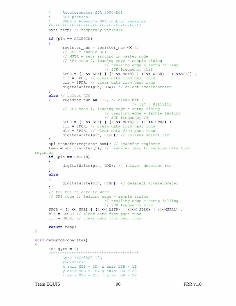
Team EQUIS 96 FRR v1.0
* Accelerometer SCA 3000-D01
* SPI protocol
* SPCR = Atmega's SPI control register
***************************************/
byte temp; // temporary variable
if (pin == ACCEPIN)
register_num = register_num << 2;
// SPE = enable SPI
// MSTR = sets arduino in master mode
// SPI mode 0, leading edge = sample rising
// trailing edge = setup falling
// SCK frequency /128
SPCR = (1 << SPE) | (1 << MSTR) | (1<< SPR0) | (1<<SPR1) ;
clr = SPCR; // clear data from past runs
clr = SPDR; // clear data from past runs
digitalWrite(pin, LOW); // select accelerometer
else // select RTC
register_num &= 127; // clear bit 7
// 127 = 01111111
// SPI mode 1, leading edge = setup rising
// trailing edge = sample falling
// SCK frequency /4
SPCR = (1 << SPE) | (1 << MSTR) | (1 << CPHA) ;
clr = SPCR; // clear data from past runs
clr = SPDR; // clear data from past runs
digitalWrite(pin, HIGH); // (slave) select rtc
spi_transfer(register_num); // transfer register
temp = spi_transfer(0); // transfer zero to receive data from
register
if (pin == RTCPIN)
digitalWrite(pin, LOW); // (slave) deselect rtc
else
digitalWrite(pin, HIGH); // deselect accelerometer
// for the sd card to work
// SPI mode 0, leading edge = sample rising
// trailing edge = setup falling
// SCK frequency /128
SPCR = (1 << SPE) | (1 << MSTR) | (1<< SPR0) | (1<<SPR1) ;
clr = SPCR; // clear data from past runs
clr = SPDR; // clear data from past runs
return temp;
void getGyroscopeData()
int gyro = 0;
/**************************************
Gyro ITG-3200 I2C
registers:
x axis MSB = 1D, x axis LSB = 1E
y axis MSB = 1F, y axis LSB = 20
z axis MSB = 21, z axis LSB = 22

Team EQUIS 97 FRR v1.0
**************************************/
// Arduino Wire library (I2C)
Wire.beginTransmission(GYRO_ADDR);
Wire.send(0x1D); // MSB x axis
Wire.endTransmission();
Wire.requestFrom(GYRO_ADDR, 1); // one byte
byte msb = 0;
byte lsb = 0;
while(!Wire.available())
// wait for data to be available
;
msb = Wire.receive();
Wire.beginTransmission(GYRO_ADDR);
Wire.send(0x1E); // LSB x axis
Wire.endTransmission();
Wire.requestFrom(GYRO_ADDR, 1); // one byte
while(!Wire.available())
// wait for data to be available
;
lsb = Wire.receive();
// calculate total x axis
gyro = (( msb << 8) | lsb);
Serial.print(" gyroX= "); Serial.print(gyro);
file.print(","); file.print(gyro);
// clear variables
msb = 0;
lsb = 0;
gyro = 0;
Wire.beginTransmission(GYRO_ADDR);
Wire.send(0x1F); // MSB y axis
Wire.endTransmission();
Wire.requestFrom(GYRO_ADDR, 1); // one byte
while(!Wire.available())
// wait for data to be available
;
msb = Wire.receive();
Wire.beginTransmission(GYRO_ADDR);
Wire.send(0x20); // LSB y axis
Wire.endTransmission();
Wire.requestFrom(GYRO_ADDR, 1); // one byte
while(!Wire.available())
// wait!
;
lsb = Wire.receive();
// calculate total y axis
gyro = (( msb << 8) | lsb);
Serial.print(" gyroX= "); Serial.print(gyro);
file.print(","); file.print(gyro);

Team EQUIS 98 FRR v1.0
// clear variables
msb = 0;
lsb = 0;
gyro = 0;
Wire.beginTransmission(GYRO_ADDR);
Wire.send(0x21); // MSB z axis
Wire.endTransmission();
Wire.requestFrom(GYRO_ADDR, 1); // one byte
while(!Wire.available())
// wait...
;
msb = Wire.receive();
Wire.beginTransmission(GYRO_ADDR);
Wire.send(0x22); // LSB z axis
Wire.endTransmission();
Wire.requestFrom(GYRO_ADDR, 1); // one byte
while(!Wire.available())
// ...
;
lsb = Wire.receive();
// calculate z axis
gyro = (( msb << 8) | lsb);
Serial.print(" gyroZ= "); Serial.println(gyro);
file.print(","); file.print(gyro);
void getTemperatureData()
/***************************
* 1-Wire digital thermometer
* DS18B20
****************************/
byte data[2]; // temperature data
tempSens.reset(); // initialization
tempSens.skip(); //Skip the device selection. This only works if you
//have a single device.
tempSens.write(0x44,1); // start conversion
delay(1000); // wait for conversion
tempSens.reset(); // initialization
tempSens.skip(); //Skip the device selection, This only works if you
//have a single device
tempSens.write(0xBE); // Read Scratchpad
file.print(",");
for ( int i = 0; i <= 2; i++)
// 3 bytes
data[i] = tempSens.read(); //read a byte
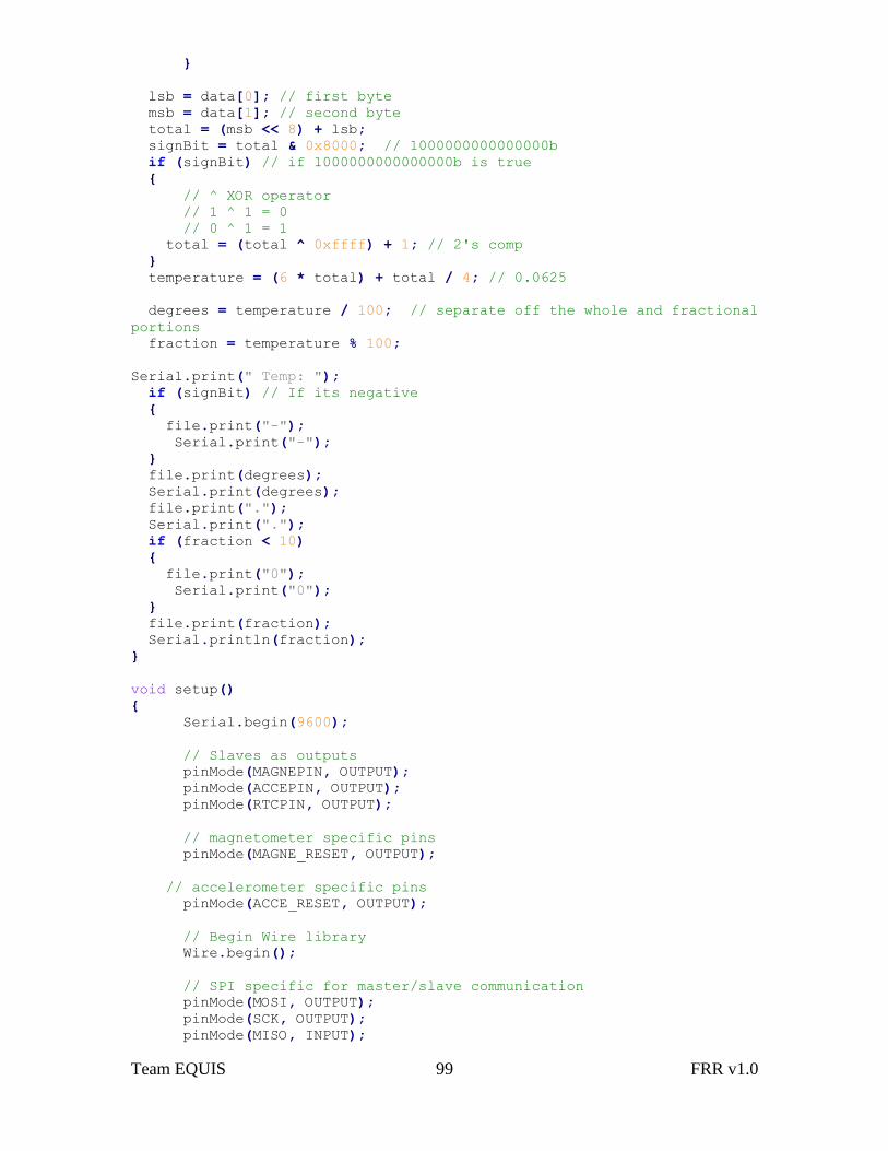
Team EQUIS 99 FRR v1.0
lsb = data[0]; // first byte
msb = data[1]; // second byte
total = (msb << 8) + lsb;
signBit = total & 0x8000; // 1000000000000000b
if (signBit) // if 1000000000000000b is true
// ^ XOR operator
// 1 ^ 1 = 0
// 0 ^ 1 = 1
total = (total ^ 0xffff) + 1; // 2's comp
temperature = (6 * total) + total / 4; // 0.0625
degrees = temperature / 100; // separate off the whole and fractional
portions
fraction = temperature % 100;
Serial.print(" Temp: ");
if (signBit) // If its negative
file.print("-");
Serial.print("-");
file.print(degrees);
Serial.print(degrees);
file.print(".");
Serial.print(".");
if (fraction < 10)
file.print("0");
Serial.print("0");
file.print(fraction);
Serial.println(fraction);
void setup()
Serial.begin(9600);
// Slaves as outputs
pinMode(MAGNEPIN, OUTPUT);
pinMode(ACCEPIN, OUTPUT);
pinMode(RTCPIN, OUTPUT);
// magnetometer specific pins
pinMode(MAGNE_RESET, OUTPUT);
// accelerometer specific pins
pinMode(ACCE_RESET, OUTPUT);
// Begin Wire library
Wire.begin();
// SPI specific for master/slave communication
pinMode(MOSI, OUTPUT);
pinMode(SCK, OUTPUT);
pinMode(MISO, INPUT);

Team EQUIS 100 FRR v1.0
//reset pins
digitalWrite(MAGNE_RESET, LOW);
digitalWrite(ACCE_RESET, HIGH);
// slaves deselected
digitalWrite(ACCEPIN, HIGH); // acce idle mode
digitalWrite(RTCPIN, LOW); // rtc idle mode
digitalWrite(MAGNEPIN, HIGH); // datasheet: HIGH = magnetometer in
idle //mode
//Setup gyroscope
initGyro();
// initialize the SD card
if (!card.init()) error("card.init");
// initialize a FAT volume
if (!volume.init(card)) error("volume.init");
// open root directory
if (!root.openRoot(volume)) error("openRoot");
// File Creation
int counter = 0; //
char fileName[] = "EQUIS000.CSV"; // file in comma separated values
//format
for (int num = 0; num < 1000; num++) // up to 999 files
fileName[5] = num/100 + '0';
if( counter >= 100)
counter = 0;
if (num >= 100)
fileName[6] = counter/10 + '0';
counter++;
if (num < 100)
fileName[6] = num/10 + '0';
fileName[7] = num % 10 +'0';
if(file.open(root, fileName, O_CREAT | O_EXCL | O_WRITE))
break;
if (!file.isOpen()) error ("file.create");
Serial.print("Logging to: ");
Serial.println(fileName);
// Sensor Headers
file.print("Date_Hr:Mm:Ss");
file.print(",mag_X"); file.print(",mag_Y"); file.print(",mag_Z"); //
3 //axis magnetometer
file.print(",acc_X"); file.print(",acc_Y"); file.print(",acc_Z"); //
3 //axis accelerometer

Team EQUIS 101 FRR v1.0
file.print(",gyr_X"); file.print(",gyr_Y"); file.print(",gyr_Z"); //
3 //axis gyroscope
file.print(",temp"); // temperature sensor
file.println(); // new line
if (file.writeError || !file.sync())
error("write header");
void loop()
file.writeError = 0;
delay((LOG_INTERVAL -1) - (millis() % LOG_INTERVAL));
// real-time clock
Serial.print("Date_Hr:Mm:Ss "); // testing
rtc_data = RTC_Acc_Data(0x04, RTCPIN); // receive date, HEX register
file.print(rtc_data, HEX); file.print("_");
Serial.print(rtc_data, HEX); Serial.print("_"); // testing
rtc_data = RTC_Acc_Data(0x02, RTCPIN); // receive hour, HEX register
file.print(rtc_data, HEX); file.print(":");
Serial.print(rtc_data, HEX); Serial.print(":"); // testing
rtc_data = RTC_Acc_Data(0x01, RTCPIN); // receive minutes, HEX
register
file.print(rtc_data, HEX); file.print(":");
Serial.print(rtc_data, HEX); Serial.print(":"); // testing
rtc_data = RTC_Acc_Data(0x00, RTCPIN); // receive seconds, HEX
register
file.print(rtc_data, HEX);
Serial.println(rtc_data, HEX); // testing
// magnetometer data
Serial.print("Mag: ");
getMagnetometerData();
Serial.println();
// accelerometer Data
byte lsb = 0;
byte msb = 0;
Serial.print("Acc: ");
msb = RTC_Acc_Data(0x05, ACCEPIN); // msb x axis
lsb = RTC_Acc_Data(0x04, ACCEPIN); // lsb x axis
acc_data = ((msb << 8) | (lsb & 0xf8)) / 8;
file.print(","); file.print(acc_data);
Serial.print("x = "); Serial.print(acc_data);
msb = RTC_Acc_Data(0x07, ACCEPIN); // msb y axis
lsb = RTC_Acc_Data(0x06, ACCEPIN); // lsb y axis
acc_data = ((msb << 8) | (lsb & 0xf8)) / 8;
file.print(","); file.print(acc_data);
Serial.print(" y = "); Serial.print(acc_data);
msb = RTC_Acc_Data(0x09, ACCEPIN); // msb z axis
lsb = RTC_Acc_Data(0x08, ACCEPIN); // lsb z axis
acc_data = ((msb << 8) | (lsb & 0xf8)) / 8;
file.print(","); file.print(acc_data);
Serial.print(" z = "); Serial.println(acc_data);
// gyroscope data
getGyroscopeData();
//Serial.println();

Team EQUIS 102 FRR v1.0
// temperature data
getTemperatureData();
file.println(); // new line
//don't sync too often - requires 2048 bytes of I/O to SD card
if ((millis() - syncTime) < SYNC_INTERVAL) return;
syncTime = millis();
if (!file.sync()) error("sync");

Team EQUIS 103 FRR v1.0
Appendix D
Shock Test Raw Data
Date_Hr:Mm:Ss mag_X mag_Y mag_Z acc_X acc_Y acc_Z gyr_X gyr_Y gyr_Z temp
22_13:43:1 -334 6 1275 241 -29 1327 3 72 -47 29.25
22_13:43:5 -262 39 1326 284 -121 1326 16 35 -21 29.31
22_13:43:9 -136 33 1304 219 -144 1323 -29 10 -15 29.25
22_13:43:13 -197 -4 1342 240 -130 1333 56 65 -78 29.31
22_13:43:17 -190 31 1236 -209 8 1382 179 306 -262 29.31
22_13:43:21 -477 -456 1248 -959 -359 288 987 3038 -1095 29.31
22_13:43:25 -470 1239 -209 -1297 -108 -223 8 33 -7 29.37
22_13:43:29 -470 1237 -209 -1299 -116 -226 10 34 -7 29.5
22_13:43:33 -470 1237 -208 -1299 -113 -224 10 34 -7 29.5
22_13:43:37 -468 1240 -208 -1296 -108 -225 9 34 -7 29.56
22_13:43:41 -469 1237 -209 -1300 -104 -235 9 33 -7 29.56
22_13:43:45 -469 1152 1280 -258 88 1444 -288 -213 721 29.62
22_13:43:49 -515 370 1185 -483 -43 1307 -10 19 283 29.56
22_13:43:53 -43 1087 794 -577 99 893 -363 172 -281 29.56
22_13:43:57 -355 -496 1051 -303 84 1305 239 120 -77 29.56
22_13:44:1 -74 -435 1116 -52 58 1335 13 100 -499 29.56
22_13:44:5 493 -332 1016 81 113 1360 -76 -200 -370 29.5
22_13:44:9 674 -59 1089 149 -61 1388 -51 88 27 29.5
22_13:44:13 648 -663 973 223 -7 1380 -65 69 -420 29.5
22_13:44:17 484 -479 1032 170 91 1356 8 38 -29 29.5
22_13:44:21 569 -291 1031 236 179 1310 85 49 -71 29.5
22_13:44:25 608 -116 1099 211 102 1346 -3 11 -9 29.5
22_13:44:29 589 -142 1095 150 132 1358 40 15 44 29.5
22_13:44:34 659 -124 1110 85 123 1363 28 66 53 29.5
22_13:44:38 644 125 1069 101 -98 1455 -304 50 -496 29.5
22_13:44:42 -645 -165 851 55 97 1350 -57 -18 19 29.5
22_13:44:46 -618 463 1006 -24 74 1363 11 35 -7 29.5
22_13:44:50 -619 461 1005 -29 72 1368 10 35 -6 29.56
22_13:44:54 -620 460 1006 -28 67 1370 11 35 -7 29.5
22_13:44:58 -620 462 1004 -26 74 1364 10 34 -6 29.5
22_13:45:2 -620 458 1003 -30 74 1351 10 35 -6 29.56
22_13:45:6 -615 472 1009 -29 73 1367 10 35 -6 29.56
22_13:45:10 -617 478 1009 -17 70 1364 10 35 -7 29.5
22_13:45:14 -614 468 1012 -24 72 1363 10 35 -5 29.56
22_13:45:18 -616 232 934 -133 129 1388 -103 -57 154 29.56
22_13:45:22 -551 191 731 79 127 1358 16 18 -36 29.56
22_13:45:26 -487 180 558 90 95 1365 -77 -12 122 29.56
22_13:45:30 -487 127 639 244 53 1330 6 58 -15 29.56
22_13:45:34 -475 -16 615 166 14 1302 -32 -76 14 29.62

Team EQUIS 104 FRR v1.0
22_13:45:38 -445 -28 453 -367 -241 3141 283 -151 -466 29.62
22_13:45:42 -477 757 1244 -35 149 1358 10 35 -6 29.56
22_13:45:46 -271 758 1238 -36 149 1354 11 35 -6 29.56
22_13:45:50 -271 757 1242 -30 146 1358 11 35 -6 29.62
22_13:45:54 -273 758 1241 -31 146 1359 11 35 -6 29.62
22_13:45:58 -273 759 1241 -41 145 1354 11 35 -6 29.62
22_13:46:2 -271 763 1253 233 144 1425 -117 59 -136 29.62
22_13:46:6 46 694 1334 -161 -13 1369 -41 -74 234 29.62
22_13:46:10 378 201 1304 -25 -6 1353 -21 26 54 29.68
22_13:46:14 626 -38 1309 -170 205 1352 156 -124 88 29.68
22_13:46:18 514 -51 1377 -9 115 1346 -37 80 -190 29.68
22_13:46:22 648 222 1297 -37 43 1350 29 -1 -58 29.68
22_13:46:26 672 283 1288 -26 19 1355 28 4 1 29.68
22_13:46:30 670 262 1361 -142 71 1404 -70 -70 43 29.68
22_13:46:34 530 75 1355 39 66 1345 -77 22 -31 29.68
22_13:46:38 581 167 1311 6 64 1383 72 -3 36 29.68
22_13:46:42 628 70 1324 75 99 1394 -127 102 258 29.68
22_13:46:46 570 -41 1358 80 192 1334 21 44 -8 29.75
22_13:46:50 512 -5 1366 79 218 1352 18 53 -7 29.75
22_13:46:54 516 -75 1347 131 178 1351 -1 49 -4 29.75
22_13:46:58 537 -81 1342 152 171 1357 57 69 -1 29.81
22_13:47:2 571 98 1303 179 -17 1314 106 112 -254 29.75
22_13:47:6 398 -515 1335 -54 41 1421 -345 111 -1139 29.81
22_13:47:10 325 633 948 -156 16 1457 40 194 133 29.81
22_13:47:14 619 -106 1161 -104 152 1384 82 83 22 29.81
22_13:47:18 662 120 1136 10 -167 1356 -1 3 687 29.81
22_13:47:22 -532 -103 827 414 -290 1267 58 474 -551 29.81
22_13:47:26 -831 1 1066 209 -40 1615 -271 176 -13 29.81
22_13:47:30 -793 -609 707 373 -110 1541 -50 -61 195 29.87
22_13:47:34 -492 -502 885 104 -9 983 216 95 87 29.87
22_13:47:38 24 -633 934 -104 216 1111 119 -137 163 29.87
22_13:47:42 -228 -635 577 -126 285 1236 -53 99 -438 29.81
22_13:47:46 -514 -540 721 -50 153 1738 -124 47 -298 29.81
22_13:47:50 -381 -689 807 49 66 994 -140 3 -103 29.87
22_13:47:54 -344 -478 368 20 -14 1330 165 -144 475 29.87
22_13:47:58 -658 387 776 146 287 1444 -1 223 -37 29.87
22_13:48:2 -554 338 668 127 247 1321 14 81 -102 29.87
22_13:48:6 -690 348 667 36 158 1354 -10 102 3 29.87
22_13:48:10 -716 208 645 15 100 1351 5 9 -12 29.93
22_13:48:14 -705 228 667 162 33 1369 -109 186 85 29.93
22_13:48:18 -640 181 659 62 226 1362 359 36 -308 29.93
22_13:48:22 -627 247 724 -23 103 1342 -47 153 -210 29.93
22_13:48:26 -724 186 572 166 -142 1352 -51 153 78 29.93
22_13:48:30 -733 345 734 -70 5 1481 -139 3 1096 30

Team EQUIS 105 FRR v1.0
22_13:48:34 441 982 704 -30 49 1367 13 36 -5 30
22_13:48:38 441 981 713 -27 43 1364 13 37 -5 30
22_13:48:42 429 967 710 -41 37 1361 19 46 -5 30
22_13:48:46 445 979 707 -33 53 1352 13 37 -5 30
22_13:48:50 446 980 764 101 163 1350 -31 14 -464 30
22_13:48:54 744 -342 778 -43 58 1363 13 36 -5 30
22_13:48:58 745 -339 772 -34 60 1362 13 38 -4 30.06
22_13:49:2 745 -331 762 -20 65 1365 14 36 -4 30.06
22_13:49:6 745 -337 787 -17 61 1368 13 36 -4 30.06
22_13:49:10 735 -333 784 -14 49 1355 13 36 -5 30.06
22_13:49:14 762 -353 770 -20 50 1353 2 18 -4 30.06
22_13:49:18 732 -334 798 -6 45 1366 10 34 -5 30.12
22_13:49:22 736 -342 785 -9 63 1366 20 47 -4 30.12
22_13:49:26 731 -336 780 1 124 1325 14 37 -4 30.12
22_13:49:30 754 -346 771 -51 58 1365 14 36 -4 30.12
22_13:49:34 761 -348 781 -21 69 1369 14 38 -4 30.18
22_13:49:38 767 -344 782 -59 37 1377 3 19 -4 30.12
22_13:49:42 760 -334 761 -20 62 1370 14 37 -4 30.18
22_13:49:46 765 -352 787 -31 58 1361 14 37 -4 30.12
22_13:49:50 766 -344 781 -17 61 1375 14 37 -4 30.18
22_13:49:54 739 -356 789 -30 67 1365 15 37 -4 30.18
22_13:49:58 747 -361 785 -18 54 1364 14 38 0 30.18
22_13:50:2 737 -370 785 -14 60 1364 15 38 -4 30.18