Haschke

7/25/2019 Haschke

http://slidepdf.com/reader/full/haschke 1/6

Simulation of Evaporating Dropletson AFM-Cantilevers

Thomas Haschke1, Daniel Lautenschlager 1, Wolfgang Wiechert1, Elmar Bonaccurso2, Hans-Jürgen Butt2

1University of Siegen, Faculty 11, Department of Simulation, 57076 Siegen, Germany,{haschke, lautenschlager, wiechert}@simtec.mb.uni-siegen.de, 2Max-Planck-Institute forPolymer Research, Polymer Physics Group, Ackermannweg 10, 55128 Mainz, Germany,{bonaccur, butt}@mpip-mainz.mpg.de

1 Introduction

The design of micro and nanoscale systems is a great challenge for modelling andsimulation. In particular Lab-on-a-Chip-technology offers a wide spectrum of possibleapplications. Because micro and nano scale systems behave very differently from macroscale systems, the behaviour of physico-chemical processes on this scale is still subject to

research. Hence several research projects for Lab-on-a-Chip-applications are run tounderstand the behaviour of these systems and get familiar with the different effects on thatscale (e. g. Cµ 2002, Nano 2002).

At least since Deegan’s publication about drying drops of coffee in Nature (Deegan et al.1997), evaporating micro droplets are a frequently investigated topic. Other authors dealtwith “special” effects like the behaviour of evaporating droplets on solid surfaces (Erbil et al.2002), fluid flow inside the drop (Hu & Larson 2002), Marangoni-Benard-instability (Nguyen &Stebe 2002) or surface morphology (Shmuylovich et al. 2002), only to mention some of them.Stupperich et al. (2005) and Cordeiro & Pakula (2005) presented simulation models for theproduction of microwells which takes into account some of the phenomena mentioned beforefrom other authors.

A general problem for many systems of drying droplets is the relatively short evaporation

time from milliseconds up to a few seconds. So it is very difficult to study the evaporationprocess and related effects. Recently Bonaccurso and Butt (Bonaccurso & Butt 2005)presented a new approach to investigate droplet evaporation: They placed water droplets onrectangular, silicon atomic force microscope (AFM) cantilevers so that the resonancefrequency and the inclination of the cantilever versus time could be measured (Fig. 1). Withthe help of these values the evaporation process can be described and conclusions aboutthe acting forces and interactions between solid, fluid and gas can be drawn.

This contribution deals with a simulation model for these experiments, the resonancefrequency analysis as well as the simulation of the evaporating droplet on the cantilever. Inthe following chapters the experimental setup and analytical basics, the simulation modeland the simulation results are presented.

2 Experimental Setup and Analytical 2D Model

As shown in Fig. 1 the water drops are placed on the cantilever with a dispenser. The liquiddrop exerts forces on the cantilever, which finally result in an upward bending free end of thebeam. The upward bending is due to the fact that on this scale mass and gravitation can beneglected and surface forces are dominating.

Excerpt from the Proceedings of the COMSOL Multiphysics User's Conference 2005 Frankfurt

7/25/2019 Haschke


Fig. 1: Evaporation sequence of a water drop on an AFM-cantilever: Images taken from anexperiment (left) and experimental data contact radius and inclination, respectively, versusevaporation time (right) taken from cantilever deflection.

Forces responsible for the deflection (Fig. 2) are, according to Bonaccurso and Butt (2005),

- Laplace pressure of the fluid: 2 / 2 sin / P R a

- Normal component of the liquid surface tension: sinnormal

- Change in surface stress of the cantilever: - Lateral component of the liquid surface tension: coslateral

- Line tension at the rim of the drop:

Here, R is the radius of curvature, a the contact radius and the contact angle between solidand liquid. With the Young’s modulus E of the cantilever and the moment of inertia I of a

rectangular cantilever (I = WH³/12; W and H are the cantilever’s width and height,respectively), the differential equation for the cantilever inclination in a simplified 2Dapproximation is given by (Bonaccurso & Butt 2005)

32

sin cos4

dz a d

dx EI a a

(1)

The first term in (1) is caused by the normal component of the liquid surface tension and the

Laplace pressure and leads to an upward bending of the cantilever towards the drop. cos ,

and act on the three-phase contact line. They hamper the bending in the lengthdirection of the cantilever and simultaneously lead to a bending in the cantilever’s width

direction. If Young’s equation is valid, the term cos - disappears because the

difference in the solid surface tensions is equal to the change in surface stress . The last

term (line tension ) and the gravity are negligible so that (1), in a first approximation, isreduced to the first term.

The analytical model (1) predicts inclinations that are about 20% higher than the inclinationsmeasured in the experiments. The reason for this discrepancy may be the fact that theanalytical 2D model does not take the deflection of the cantilever in its width direction intoaccount. This deflection in width direction leads to a stiffer cantilever and so to a smallerinclination. Hence a 3D simulation model with FEMLAB which considers this effect is set up.

The resonance frequency of the cantilever with (f i ) and without (f 0 ) a drop is calculated fromthe analytical model by (Bonaccurso & Butt 2005) as


7/25/2019 Haschke


0 2

1 10.1614

2 0.243 2 0.243i

i

K H E K f f

M L m M

(2)

Here, K is the spring constant calculated with K = EWH³/4L² , L the cantilever’s length, itsdensity and M its mass. The two equations are basically alike, but for the mass mi of thedrop, which is added to the mass of the cantilever. Again this has to be considered in the 3D

simulation in FEMLAB.

3 Simulation Models

The experiments are divided into three parts and therewith three different simulation models.The main focus is of course on the simulation of the cantilever bending. On the other handthe determination of the resonance frequency with and without a drop on the cantilever,respectively, plays a role, too. For the simulation, 3D-FEMLAB models (structural mechanicsmodule) were set up which take into account the cantilever geometry, the drop propertiesand the above mentioned forces.

Fig. 2: Forces causing the deflection (left) and simulation for a cantilever with fixed left side (right).

The cantilever, with given dimensions (L, W, H ) and material properties (E , and Poisson’s

ratio ) is modelled as a rectangular solid in Cartesian coordinates in all three models. Theleft side of the cantilever is fixed (Rx, Ry, Rz = 0 ) and the contact area of the drop is placedas a circle on an embedded workplane at the solid (Fig. 2). Because of the critical ratio oflength and width to height, the mesh in all models is scaled in z -direction with the factor 7 .

3.1 Simulation of the Cantilever Bending

The bending of the cantilever is simulated at discrete times, at which also the contact radius,the contact angle and the inclination were measured (compare Fig. 1). The model takes onlythe Laplace pressure and the normal component of the liquid surface tension into account(see (1)). The contact area is defined by the contact radius a and the middle of the drop in x -direction. In y -direction the drop’s center is placed on the middle line. The Laplace pressureis defined as force per area on the contact area in negative z -direction. The three-phasecontact line is represented by the border of the contact area. Here the normal component of

the liquid surface tension is set as force per length in positive z -direction. For the solutionprocess two steps of grid adaptation with a maximum of 10 6 cells are allowed.

To evaluate the simulation, the simulated inclination of the cantilever has to be comparedwith the measured one. For this purpose a MATLAB routine is used which calculates theinclination between adjacent points in cantilever’s length direction. Therefore a fine meshgridof points is laid on the cantilever’s top and the displacements in z -direction at these pointsare computed with the postinterp-command. In a last step the difference between thecalculated inclinations from the free to the fixed end of the beam are summarized. If the sum

of differences exceeds a defined tolerance , the summation is stopped and the mean of the


7/25/2019 Haschke


inclinations from the fixed end up to this point is calculated. This way, several meaninclinations in cantilever’s length direction are calculated. The simulated inclination is finallyset to the mean of all determined inclinations in x -direction.

3.2 Simulation of the Resonance Frequencies

The simulation of the resonance frequency of the unstressed cantilever gives above all theproof that the experiment can be simulated with satisfying results in FEMLAB. In particularthe scaling of the mesh with factor 7 due to the dimension’s ratio is critical and has to berevised. For this purpose the cantilever’s resonance frequency with the described setup iscomputed without grid adaptation in the resonance frequency mode.

For the validation of the model also the stressed cantilever is simulated. In this experimentthe impact of the drop and the resulting initial resonance frequency is measured. Hence onlythe drop’s mass just before the impact and the location of the impact, i.e. the x -location, areimportant. Instead of a spherical cap we used a cylinder with the same volume as the fallingdrop before the impact on the cantilever and the contact radius measured in the experiments.The Poisson’s Ratio of the water drop was set to 0.25 , the density to 1000 kg/m³ and theYoungs’s Modulus to 0.015 GPa, i.e. the Young’s Modulus of rubber, so that the cantilever’s

stiffness is not increased through the additional mass. Again no grid adaptation is allowed.

3.3 Parameter Studies and Sensitivity Analysis

For the purpose of parameter studies and sensitivity analysis the FEMLAB-models areparameterized so that the simulations can be controlled with MATLAB. Hence thecantilever’s dimensions and properties, the experimental data and the forces are set as

variables. In the first place the material properties of the cantilever (E, , ), but also thecantilever’s height H are varied to investigate their influence on the cantilever’s inclination.The aim of these studies is a verification of the underlying models for the cantilever bendingdue to droplet evaporation on micro and nano scales.

4 Results

The simulations described in sections 3.1 and 3.2 were made for three different experimentseach, i.e. there are three different evaporation sequences and three resonance frequencies,each with and without drop. The results of the parameter studies (section 3.3) are presentedfor one cantilever.

4.1 Simulation of the Cantilever Bending

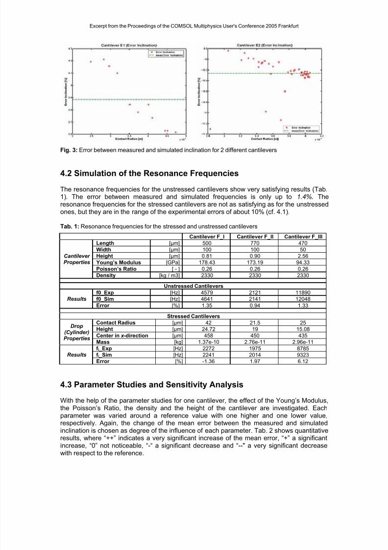
The results of the simulation are in good agreement with the experiment (see section 3). Assuming that the deflection of the cantilever can be described in a first approach by (1) wesee a nearly constant error between the measured and simulated inclination for all threecantilevers. The mean error variation from +4% (Cantilever E1, cf. Fig. 3) to -12% (CantileverE3) can be due to the measurement errors in the experiments, or to wrong materialparameters (see section 4.3).


7/25/2019 Haschke


Fig. 3: Error between measured and simulated inclination for 2 different cantilevers

4.2 Simulation of the Resonance Frequencies

The resonance frequencies for the unstressed cantilevers show very satisfying results (Tab.1). The error between measured and simulated frequencies is only up to 1.4%. Theresonance frequencies for the stressed cantilevers are not as satisfying as for the unstressedones, but they are in the range of the experimental errors of about 10% (cf. 4.1).

Tab. 1: Resonance frequencies for the stressed and unstressed cantilevers

Cantilever F_I Cantilever F_II Cantilever F_III

Length [µm] 500 770 470

Width [µm] 100 100 50

Height [µm] 0.81 0.90 2.56

Young’s Modulus [GPa] 178.43 173.19 94.33

Poisson’s Ratio [ - ] 0.26 0.26 0.26

CantileverProperties

Density [kg / m3] 2330 2330 2330

Unstressed Cantilevers

f0_Exp [Hz] 4579 2121 11890

f0_Sim [Hz] 4641 2141 12048Results

Error [%] 1.35 0.94 1.33

Stressed Cantilevers

Contact Radius [µm] 42 21.5 25

Height [µm] 24.72 19 15.08

Center in x -direction [µm] 458 450 435

Drop(Cylinder)Properties

Mass [kg] 1.37e-10 2.76e-11 2.96e-11

f i _Exp [Hz] 2272 1975 8785

f i _Sim [Hz] 2241 2014 9323Results

Error [%] -1.36 1.97 6.12

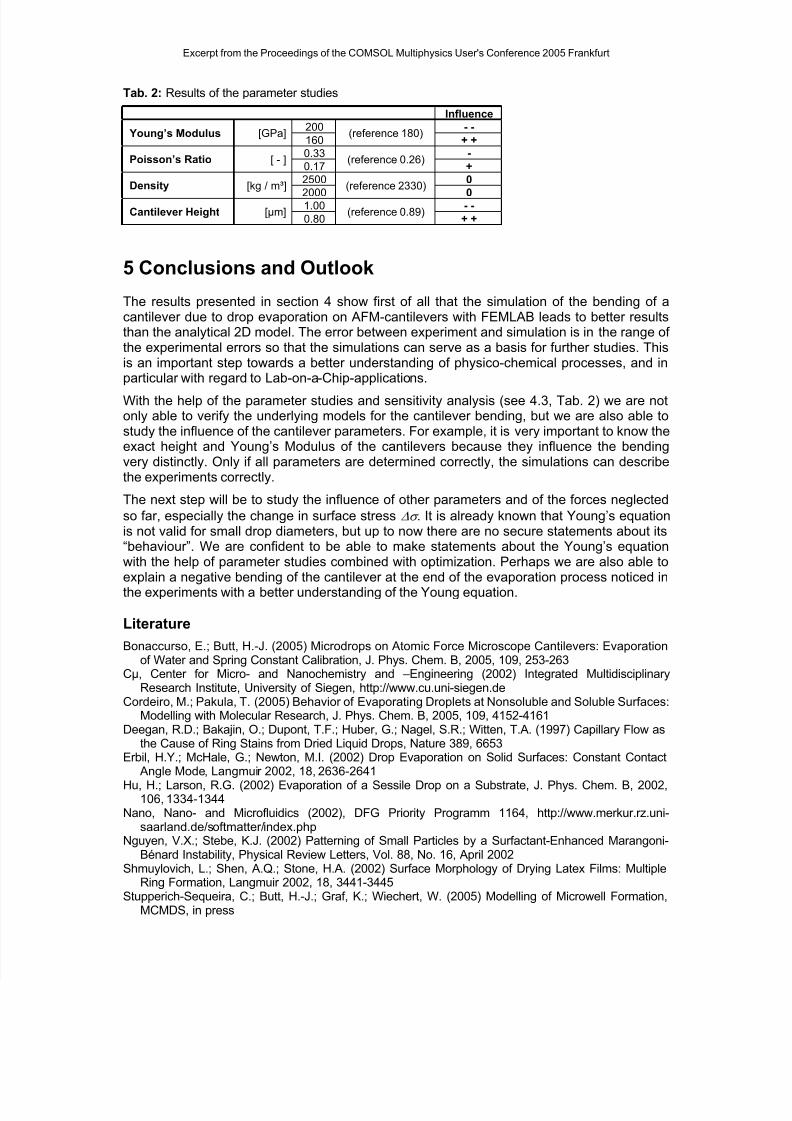
4.3 Parameter Studies and Sensitivity Analysis

With the help of the parameter studies for one cantilever, the effect of the Young’s Modulus,the Poisson’s Ratio, the density and the height of the cantilever are investigated. Eachparameter was varied around a reference value with one higher and one lower value,respectively. Again, the change of the mean error between the measured and simulatedinclination is chosen as degree of the influence of each parameter. Tab. 2 shows quantitativeresults, where “++” indicates a very significant increase of the mean error, “+” a significantincrease, “0” not noticeable, “-“ a significant decrease and “--" a very significant decreasewith respect to the reference.


7/25/2019 Haschke


Tab. 2: Results of the parameter studies

Influence

200 - - Young’s Modulus [GPa]

160(reference 180)

+ +

0.33 -Poisson’s Ratio [ - ]

0.17(reference 0.26)

+

2500 0Density [kg / m³]

2000

(reference 2330)

01.00 - -Cantilever Height [µm]

0.80(reference 0.89)

+ +

5 Conclusions and Outlook

The results presented in section 4 show first of all that the simulation of the bending of acantilever due to drop evaporation on AFM-cantilevers with FEMLAB leads to better resultsthan the analytical 2D model. The error between experiment and simulation is in the range ofthe experimental errors so that the simulations can serve as a basis for further studies. Thisis an important step towards a better understanding of physico-chemical processes, and inparticular with regard to Lab-on-a-Chip-applications.

With the help of the parameter studies and sensitivity analysis (see 4.3, Tab. 2) we are notonly able to verify the underlying models for the cantilever bending, but we are also able tostudy the influence of the cantilever parameters. For example, it is very important to know theexact height and Young’s Modulus of the cantilevers because they influence the bendingvery distinctly. Only if all parameters are determined correctly, the simulations can describethe experiments correctly.

The next step will be to study the influence of other parameters and of the forces neglected

so far, especially the change in surface stress . It is already known that Young’s equationis not valid for small drop diameters, but up to now there are no secure statements about its“behaviour”. We are confident to be able to make statements about the Young’s equationwith the help of parameter studies combined with optimization. Perhaps we are also able toexplain a negative bending of the cantilever at the end of the evaporation process noticed in

the experiments with a better understanding of the Young equation.

Literature

Bonaccurso, E.; Butt, H.-J. (2005) Microdrops on Atomic Force Microscope Cantilevers: Evaporationof Water and Spring Constant Calibration, J. Phys. Chem. B, 2005, 109, 253-263

Cµ, Center for Micro- and Nanochemistry and –Engineering (2002) Integrated MultidisciplinaryResearch Institute, University of Siegen, http://www.cu.uni-siegen.de

Cordeiro, M.; Pakula, T. (2005) Behavior of Evaporating Droplets at Nonsoluble and Soluble Surfaces:Modelling with Molecular Research, J. Phys. Chem. B, 2005, 109, 4152-4161

Deegan, R.D.; Bakajin, O.; Dupont, T.F.; Huber, G.; Nagel, S.R.; Witten, T.A. (1997) Capillary Flow asthe Cause of Ring Stains from Dried Liquid Drops, Nature 389, 6653

Erbil, H.Y.; McHale, G.; Newton, M.I. (2002) Drop Evaporation on Solid Surfaces: Constant Contact Angle Mode, Langmuir 2002, 18, 2636-2641

Hu, H.; Larson, R.G. (2002) Evaporation of a Sessile Drop on a Substrate, J. Phys. Chem. B, 2002,106, 1334-1344

Nano, Nano- and Microfluidics (2002), DFG Priority Programm 1164, http://www.merkur.rz.uni-saarland.de/softmatter/index.php

Nguyen, V.X.; Stebe, K.J. (2002) Patterning of Small Particles by a Surfactant-Enhanced Marangoni-Bénard Instability, Physical Review Letters, Vol. 88, No. 16, April 2002

Shmuylovich, L.; Shen, A.Q.; Stone, H.A. (2002) Surface Morphology of Drying Latex Films: MultipleRing Formation, Langmuir 2002, 18, 3441-3445

Stupperich-Sequeira, C.; Butt, H.-J.; Graf, K.; Wiechert, W. (2005) Modelling of Microwell Formation,MCMDS, in press


Haschke

Documents

Transcript of Haschke