Hasan Mohseni - digital.library.adelaide.edu.au · a graphical representation for debonding...
145
Damage Identification in FRP-Retrofitted Concrete Structures Using Linear and Nonlinear Guided Waves By Hasan Mohseni Thesis submitted in fulfilment of the requirements for the degree of Doctor of Philosophy The University of Adelaide School of Civil, Environmental and Mining Engineering Faculty of Engineering, Computer and Mathematical Sciences June 2018
Transcript of Hasan Mohseni - digital.library.adelaide.edu.au · a graphical representation for debonding...

Damage Identification in FRP-Retrofitted Concrete
Structures Using Linear and Nonlinear Guided Waves
By
Hasan Mohseni
Thesis submitted in fulfilment of the requirements for the degree of
Doctor of Philosophy
The University of Adelaide
School of Civil, Environmental and Mining Engineering
Faculty of Engineering, Computer and Mathematical Sciences
June 2018


I
Abstract
Structural health monitoring (SHM) involves the implementation of damage identification
methods in engineering structures to ensure structural safety and integrity. The paramount
importance of SHM has been recognised in the literature. Among different damage
identification methods, guided wave approach has emerged as a revolutionary technique.
Guided wave-based damage identification has been the subject of intensive research in the past
two decades. Meanwhile, applications of fibre reinforced polymer (FRP) composites for
strengthening and retrofitting concrete structures have been growing dramatically. FRP
composites offer high specific stiffness and high specific strength, good resistance to corrosion
and tailorable mechanical properties. On the other hand, there are grave concerns about long-
term performance and durability of FRP applications in concrete structures. Therefore, reliable
damage identification techniques need to be implemented to inspect and monitor FRP-
retrofitted concrete structures.
This thesis aims to explore applications of Rayleigh wave for SHM in FRP-retrofitted
concrete structures. A three-dimensional (3D) finite element (FE) model has been developed
to simulate Rayleigh wave propagation and scattering. Numerical simulation results of
Rayleigh wave propagation in the intact model (without debonding at FRP/concrete interface)
are verified with analytical solutions. Propagation of Rayleigh wave in the FRP-retrofitted
concrete structures and scattering of Rayleigh waves at debonding between FRP and concrete
are validated with experimental measurements. Very good agreement is observed between the
FE results and experimental measurements. The experimentally and analytically validated FE
model is then used in numerical case studies to investigate the scattering characteristic. The

II
scattering directivity pattern (SDP) of Rayleigh wave is studied for different debonding size
to wavelength ratios and in both backward and forward scattering directions. The suitability
of using bonded mass to simulate debonding in the FRP-retrofitted concrete structures is also
investigated. Besides, a damage localisation method is introduced based on the time-of-flight
(ToF) of the scattered Rayleigh wave. Numerical case studies, involving different locations
and sizes of debonding, are presented to validate the proposed debonding localisation method.
Nonlinear ultrasonics is a novel and attractive concept with the potential of baseline-free
damage detection. In this thesis, nonlinear Rayleigh wave induced at debondings in FRP-
retrofitted concrete structures, is studied in detail. Numerical results of nonlinear Rayleigh
wave are validated with experimental measurements. The study considers both second and
third harmonics of Rayleigh wave. A very good agreement is observed between numerical and
experimental results of nonlinear Rayleigh wave. Directivity patterns of second and third
harmonics for different debonding size to the wavelength ratios, and in both backward and
forward scattering directions, are presented. Moreover, a damage image reconstruction
algorithm is developed based on the second harmonic of Rayleigh wave. This method provides
a graphical representation for debonding detection and localisation in FRP-retrofitted concrete
structures. Experimental case studies are used to demonstrate the performance of the proposed
technique. It is shown that the proposed imaging method is capable of detecting the debonding
in the FRP-retrofitted concrete structures.
Overall, this PhD study proves that Rayleigh wave is a powerful and reliable means of
damage detection and localisation in FRP-retrofitted concrete structures.

III
Acknowledgements
I am deeply honoured and privileged to have been able to undertake this PhD research. I feel
the most sincere gratitude towards my main supervisor; Associate Professor Ching-Tai Ng;
whose tremendous support and invaluable guidance led me throughout this postgraduate
journey. His extensive technical expertise along with genuine enthusiasm helped me complete
this study.
Besides, I need to extend my heartfelt appreciation to my co-supervisor; Dr. Togay
Ozbakkaloglu; who provided me with precious advice and technical support.
I would also like to thank gratefully the following people:
My fellow postgraduate students and academics at the school of civil, environmental and
mining engineering;
Technical and office staff at the faculty of engineering, computer and mathematical sciences;
And;
My Parents; who offered me enthusiastic and wholehearted support.
Hasan Mohseni
June 2018

IV


VI

VII
Table of contents
1 Introduction 1
1.1 Structural Health Monitoring 1
1.2 Guided waves 2
1.3 Fibre reinforced polymer composites 4
1.4 Objective and aims of the research 5
1.5 Thesis outline 5
1.6 List of publications 8
2 Literature review 9
2.1 Damage identification using guided waves 9
2.1.1 Fundamentals of guided waves 9
2.1.2 Generating and sensing of guided waves 12
2.1.3 Digital signal processing 14
2.1.3.1 Hilbert transform 14
2.1.3.2 Fourier transform 15
2.1.3.3 Short-time Fourier transform 15
2.1.3.4 Wavelet transform 16
2.1.4 Guided waves in composites 17
2.1.5 Waves interaction with delamination in composites 21
2.2 Structural health monitoring of FRP-retrofitted concrete structures 24
2.2.1 Applications of FRP in concrete structures 24

VIII
2.2.2 Importance of SHM in FRP-retrofitted concrete structures 25
2.2.3 Visual testing 27
2.2.4 Impact testing 28
2.2.5 Microwave method 29
2.2.6 Infrared thermography 30
2.2.7 Acoustic emission 31
2.2.8 Guided waves in FRP-retrofitted concrete structures 32
2.2.9 Rayleigh waves in concrete structures 33
2.2.10 Nonlinear Rayleigh waves 34
2.3 Conclusions and research gaps 35
3 Research Methodology 36
3.1 Explicit numerical simulations 36
3.2 Analytical solution 38
3.3 Preparation of FRP-retrofitted concrete experimental specimens 39
4 Scattering of linear Rayleigh wave 43
4.1 Finite element model description 43
4.2 Absorbing regions to improve the computational efficiency in scattering
analysis
46
4.3 Attenuation of Rayleigh wave signals 49
4.4 Analytical validation of numerical model 50
4.5 Experimental validation 52
4.5.1 Equipment setup 52
4.5.2 Validation of Rayleigh wave propagation 53

IX
4.5.3 Rayleigh wave scattering at bonded mass 58
4.6 Scattering of Rayleigh wave at debonding at FRP/concrete interface 60
4.6.1 Effect of rebars 61
4.6.2 Effect of debonding size and shape 62
5 Scattering of nonlinear Rayleigh wave 68
5.1 Numerical model 68
5.2 Validation of numerical model 69
5.2.1 Analytical verification 69
5.2.2 Equipment setup 70
5.2.3 Higher harmonics generation due to contact nonlinearity at debonding 71
5.2.4 Accuracy of the element type in simulating higher harmonics 74
5.3 Directivity patterns of higher harmonics generated at debondings 75
6 Debonding localisation in FRP-retrofitted concrete based on scattering of
linear Rayleigh wave
82
6.1 Basics of debonding localisation method 82
6.2 Numerical model description 85
6.3 Numerical case studies 87
7 Locating debonding in FRP-retrofitted concrete using nonlinear Rayleigh wave 95
7.1 Debonding detection method using nonlinear Rayleigh wave 95
7.2 Experimental studies 100
7.2.1 Experiment equipment setup 100
7.2.2 Results and discussion 102
8 Conclusions and suggestions for future research 108

X
8.1 Conclusions 108
8.2 Suggestions for further research 112
9 References 113

XI
List of figures
Figure 1-1. Examples of damage in composites a. surface cut; b. filament
breakage; c. impact dent; d. blister; e. surface swelling-blistering; and f. voids in
resin filler [3]
2
Figure 1-2. a. Rayleigh wave; b. Love wave; and c. Lamb wave [6] 3
Figure 1-3. a. Bulk waves; and b. guided waves [13] 4
Figure 2-1. Phase velocity of Lamb wave modes in a steel plate as a function of
product of frequency and thickness
11
Figure 2-2. Different sizes of PZT elements [28] 13
Figure 2-3. Typical inspection tools for visual testing and hammer tapping [77] 29
Figure 2-4. Microwave apparatus for inspection of concrete members retrofitted
with FRP composites [77].
30
Figure 2-5. a. Heating a concrete column wrapped with FRP composites; and b.
IRT image showing areas of debonding [82]
31
Figure 2-6. Schematic diagram of acoustic emission method. Courtesy of
www.nde-ed.org.
32
Figure 3-1. a. Schematic of FRP-retrofitted concrete with rebars ; b. formwork
preparation; c. concrete pour; d. preparation of carbon fabric and epoxy resin; e.
saturating carbon fabric with epoxy resin; and f. applying carbon fibre on concrete
specimen
41
Figure 4-1. Schematic diagram of the FRP-retrofitted concrete FE model 45

XII
Figure 4-2. Typical contour snapshots of out-of-plane displacement for numerical
FRP-retrofitted concrete model with a circular debonding at FRP/concrete
interface a. before Rayleigh wave reach debonding; and b. after interaction of
Rayleigh wave with debonding.
46
Figure 4-3. Schematic diagram of absorbing regions for wave scattering studies 48
Figure 4-4. Typical contour snapshots of out-of-plane displacement for Rayleigh
wave in FRP-retrofitted concrete model without and with absorbing layers a.
when the incident wave interacts with the boundary; b. soon after the wave
reflection; c. when the incident wave is being absorbed by the absorbing region;
and d. soon after the wave absorption.
49
Figure 4-5. Numerical and analytical values of group and phase velocity 51
Figure 4-6. Analytical and numerical mode shapes for FRP-retrofitted concrete
model
52
Figure 4-7. Schematic diagram of the experimental setup using 3D laser 53
Figure 4-8. FE calculated and experimentally measured Rayleigh wave signals
for concrete specimen 1 (without rebar)
54
Figure 4-9. FE calculated and experimentally measured Rayleigh wave signals
for concrete specimen 2 (with rebar)
55
Figure 4-10. Polar directivity of the normalised amplitude of Rayleigh incident
wave measured on a circular path with r = 50mm, 0° ≤ θ ≤ 360° and the actuator
located at the centre.
56
Figure 4-11. Experimental measurements using 3D laser Doppler vibrometer 57
Figure 4-12. Attenuation of Rayleigh waves in FRP-retrofitted concrete. 57

XIII
Figure 4-13. Normalised polar directivity pattern for the measured signal, with
and without cubic 40mm bonded mass.
59
Figure 4-14. SDP for a cubic 40mm bonded mass. 60
Figure 4-15. Effect of rebars on Rayleigh wave propagation. 61
Figure 4-16. SDP for 40mm×40mm rectangular debonding and 40mm diameter
circular debonding.
63
Figure 4-17. Normalised amplitude for the forward scattering of rectangular
debonding as a function of debonding size to wavelength ratio.
64
Figure 4-18. Normalised amplitude for the forward scattering of circular
debonding as a function of debonding diameter to wavelength ratio.
65
Figure 4-19. Normalised amplitude for the backward scattering of rectangular
debonding as a function of debonding size to wavelength ratio.
66
Figure 4-20. Normalised amplitude for the backward scattering of circular
debonding as a function of debonding diameter to wavelength ratio.
67
Figure 5-1. Numerical and analytical results of the Rayleigh wave phase velocity 70
Figure 5-2. Schematic diagram of experimental setup 71
Figure 5-3. Experimental validation of FE simulated linear Rayleigh wave results 72
Figure 5-4. Experimental validation of FE simulated higher harmonics 74
Figure 5-5. Comparison between the FE simulations using reduced integration
elements and full integration elements
75
Figure 5-6. Energy density spectrum in time-frequency domain for a. debonding
size of 38×38 mm and θ =30°; and b. debonding size of 22×22 mm and θ =330°
76

XIV
Figure 5-7. Directivity pattern for second harmonic amplitude to fundamental
harmonic amplitude ratio (A2/A1) in the model with debonding size 38mm ×
38mm
77
Figure 5-8. Directivity pattern for third harmonic amplitude to fundamental
harmonic amplitude ratio (A3/A1) in the model with debonding size 22mm ×
22mm
77
Figure 5-9. Second harmonic amplitude to fundamental harmonic amplitude ratio
(A2/A1) in the forward scattering direction as a function of debonding size to
wavelength ratio
78
Figure 5-10. Third harmonic amplitude to fundamental harmonic amplitude ratio
(A3/A1) in the forward scattering direction as a function of debonding size to
wavelength ratio
79
Figure 5-11. Second harmonic amplitude to fundamental harmonic amplitude
ratio (A2/A1) in the backward scattering direction as a function of debonding size
to wavelength ratio
80
Figure 5-12. Third harmonic amplitude to fundamental harmonic amplitude ratio
(A3/A1) in backward scattering direction as a function of debonding size to
wavelength ratio
80
Figure 6-1. Schematic diagram of 1D damage localization in FRP-retrofitted
concrete using ToF
83
Figure 6-2. Schematic diagram of damage localization in FRP-retrofitted concrete
element using a pair of actuator/sensor
84
Figure 6-3. FE model of FRP-retrofitted concrete 88

XV
Figure 6-4. PZT and debonding locations in Cases 1-3 of the numerical studies 88
Figure 6-5. Wave signals generated by PZT-1 and captured by PZT-3 in the model
without rebars a. signal from model without debonding; b. signal from model with
debonding; and c. scattered signal obtained from baseline subtraction
89
Figure 6-6. Wave signals generated by PZT-1 and captured by PZT-3 in the model
with rebars a. signal from model without debonding; b. signal from model with
debonding; and c. scattered signal obtained from baseline subtraction
91
Figure 6-7. Wave signals generated by PZT-4 and captured by PZT-3 for
debonding Case 4
92
Figure 6-8. Elliptic solutions for 6mm diameter circular debonding in a. Case 1;
b. Case 2; and c. Case 3
93
Figure 6-9. Elliptic solutions for 8mm diameter circular debonding in Case 4 93
Figure 7-1. a. Rayleigh wave propagation and scattering at debonding between
CFRP and concrete interface; and b. discretization of inspection area by image
pixels
96
Figure 7-2. Schematic diagram of the proposed damage debonding method and
signal processing
100
Figure 7-3. Schematic diagram of the CRFP-retrofitted concrete block and the
layout of the surface-mounted transducer array (top view) a. concrete specimen 3
with 60mm×60mm debonding; and b. concrete specimen 4 with 40mm×300mm
debonding
101
Figure 7-4. Experiment setup for one of the scanning processes in the sequential
scan
101

XVI
Figure 7-5. Measured data of signal path T1-T4 with debonding size 60mm ×
60mm
102
Figure 7-6. Energy density spectrum in time-frequency domain for the data of
signal path T1-T4 with debonding size 60mm × 60mm
103
Figure 7-7. Normalised spectral amplitude of signal path T1-T4 at fundamental
frequency and second harmonic frequency for debonding size 60mm × 60mm
103
Figure 7-8. Angular dependence of group velocity in m/s for the CFRP-retrofitted
concrete
105
Figure 7-9. Typical image of actuator/sensor signal paths T1-T4 for debonding
size 60mm × 60mm
105
Figure 7-10. a. Debonding location image; and b. corresponding binary image for
debonding size 60mm × 60mm (Circles: PZT transducers, dashed line: actual
debonding location and size, cross: centroid of the binary image)
106
Figure 7-11. a. Debonding location image; and b. corresponding binary image for
debonding size 40mm × 300mm (Circles: PZT transducers, dashed line: actual
debonding location and size)
107

XVII
List of tables
Table 2-1. Comparison of typical properties of three types of FRP with steel [68] 25
Table 2-2. Stages of application of FRP on concrete structures and different
causes of defect [20]
26
Table 4-1. Elastic properties of each FRP lamina 44
Table 6-1. Elastic properties of carbon fibre and epoxy resin 86
Table 6-2. Mechanical properties of each FRP ply 87
Table 6-3. Coordinates of the PZT centres in numerical case studies 90
Table 6-4. Coordinates of the debonding centres and diameters in numerical case
studies
90


1
1 Introduction
1.1 Structural Health Monitoring
Engineering structures are indispensable assets of the society and provide people with crucial
services. Therefore, integrity, serviceability and safety of the engineering structures are of
paramount importance. The literature on Structural Health Monitoring (SHM) has been
developed extensively over the past two decades [1, 2]. SHM is defined as the implementation
of an integrated sensing/actuating system in engineering structures in order to monitor
structural conditions and identify damage through data acquisition and processing. Damage
can be defined as any local variation in the physical state or mechanical properties of a
structural component, which can adversely affect the structural behaviour [3]. Depending on
the material, fabrication and geometry of the structure, different types of damage can occur;
e.g. cracks and fractures, buckling, corrosion, joint loosening, matrix cracking, fibre pull-out
or breakage, delamination and debonding [4]. Some common types of damage in composites
are shown in Figures 1-1a to 1-1f. The procedure of damage identification can be divided into
four levels [5]:
• Detecting the existence of damage
• Determining damage location
• Identifying damage type
• Quantifying extent or severity of the damage
It should be noted that it is more difficult and challenging to achieve higher level of damage
identification. The development and use of accurate, reliable and economical damage detection

2
techniques can enhance structural safety, integrity and serviceability. In this regard, a wide
variety of damage identification methods have been developed in the literature.
a b c
d e f
Figure 1-1. Examples of damage in composites a. surface cut; b. filament breakage; c. impact dent; d.
blister; e. surface swelling-blistering; and f. voids in resin filler [3]
1.2 Guided waves
Guided waves propagate in solid media and their propagation is characterised by the
boundaries of the waveguide. Different types of guided waves can occur in different types of
structures, depending on geometry and boundary conditions of structural element(s). Some
types of guided waves are shown in Figure 1-2 and they are listed as below.
• Rayleigh waves, also defined as surface waves, propagate along the surface of a semi-
infinite solid medium.

3
• Love waves also propagate in a semi-infinite solid medium in which direction of particle
vibration is horizontal and perpendicular to the propagation direction.
• Lamb waves propagate in a plate or plate-like thin medium.
a b c
Figure 1-2. a. Rayleigh wave; b. Love wave; and c. Lamb wave [6]
Guided wave damage identification methods have significantly captured interests of
researchers in the past two decades [7-9]. The advantages of guided waves over conventional
bulk wave inspection methods can be enumerated as follows [10-13]:
• Guided waves can propagate over relatively long distances while conventional bulk
waves can inspect only a limited area of structure from a single probe location. This is
schematically shown in Figures 1-3a and 1-3b.
• Guided waves are economical because their application is fast, energy-efficient and cost-
effective.
• Guided waves have active nature, which enables clients to apply them wherever and
whenever necessary.
• Guided waves have ability to inspect inaccessible, encapsulated and embedded structural
elements.
• Guided waves have great sensitivity to different types of damage.

4
a b
Figure 1-3. a. Bulk waves; and b. guided waves [13]
1.3 Fibre reinforced polymer composites
Fibre reinforced polymer (FRP) composites have been extensively used for retrofitting,
strengthening and repairing concrete structures [14]. The use of FRPs is economical and they
have high specific strength and high specific stiffness [15]. They, besides, show better
resistance to corrosion than other conventional construction materials such as steel. There are,
on the other hand, grave concerns about long-term performance of FRPs on concrete structures
[16-18]. That is in part because FRP is still a relatively new concept compared to other
conventional structural materials, such as steel and concrete. In addition, for FRP bonded to
concrete, experimental data on durability is sparse and not well-documented [19].
Different types of defects can occur during preparation, installation and service life of
concrete structures retrofitted by FRP composites [20]. Several non-destructive evaluation
(NDE) techniques, such as impact testing, infrared thermography and acoustic emission are
currently implemented in FRP-retrofitted concrete structures [21]. Due to the active nature of
guided waves and their above-mentioned advantages, guided wave-based method seems
promising for damage identification in FRP-retrofitted concrete structures; particularly;
debonding detection at FRP/concrete interface. To date, different approaches have been

5
adopted by researchers towards guided wave-based damage detection in homogenous and
composite materials, which will be discussed in the literature review.
1.4 Objective and aims of the research
The main objective of this research is to gain physical insights and develop guided wave-based
damage identification techniques for FRP-retrofitted concrete structures. Guided waves
propagate in FRP-retrofitted concrete structures as Rayleigh wave. Therefore, to achieve the
main objective, the following aims have been pursued:
• To gain physical insights into Rayleigh wave propagation in FRP-retrofitted concrete
structures and scattering at debonding at FRP/concrete interface.
• To enhance understanding about higher harmonics generation of Rayleigh wave due to
interaction with debonding between FRP and concrete.
• To develop a debonding localisation method in FRP-retrofitted concrete structures using
linear Rayleigh wave.
• To develop a debonding detection technique in FRP-retrofitted concrete structures using
higher harmonics of Rayleigh wave.
1.5 Thesis outline
Chapter 1 (current chapter) provides an introduction, and objective and aims of this research.
A general explanation of SHM and the use of guided wave for damage identification is
provided. Applications of FRP composites to retrofit concrete structures and defects in FRP-
retrofitted concrete structures are then discussed. A list of publications, including journal and
conference papers, is also mentioned at the end of this chapter.

6
Chapter 2 presents a comprehensive literature review in two sections. The first section
reviews applications of guided waves for damage identification, particularly in composite
structures. Various aspects of guided wave-based damage identification are discussed. The
second section reviews applications of FRP composites in concrete structures, defects in FRP-
retrofitted concrete structures, and current inspection methods for FRP-retrofitted concrete
structures. Based on the literature review, the research gaps are then identified.
Chapter 3 discusses the proposed research methodology and the basics of numerical methods
for simulation of Rayleigh wave propagation and scattering. Besides, the analytical solution
for verification of Rayleigh wave propagation is described. The preparation steps of FRP-
retrofitted concrete specimens are also presented in this chapter.
Chapter 4 presents a study of Rayleigh wave propagation in FRP-retrofitted concrete
structures and scattering of linear Rayleigh wave at debonding between FRP and concrete.
Numerical simulations of Rayleigh wave propagation and scattering are presented and
validated with analytical solutions and experimental measurements. Absorbing layers are
developed to enhance computational efficiency of numerical simulations. Furthermore, this
chapter discusses the suitability of bonded masses to simulate debonding at FRP/concrete
interface. To investigate effects of debonding size and shape on Rayleigh wave scattering, a
parametric study is also presented.
Chapter 5 provides insights into generation of higher harmonics of Rayleigh wave due to
contact nonlinearity at debondings in FRP-retrofitted concrete structures. Numerical
simulations of linear and nonlinear components of Rayleigh waves are validated with
experimental measurements. Generation of both second and third harmonics of Rayleigh wave

7
are investigated and validated with experiments. A parametric study is also carried out to
investigate the directivity patterns of second and third harmonics of Rayleigh waves for
different sizes of debonding at FRP/concrete interface.
Chapter 6 presents a debonding detection method in FRP-retrofitted concrete structures based
on the scattering of linear Rayleigh wave. The proposed method employs time-of-flight of the
scattered Rayleigh waves at debonding at FRP/concrete interface. Numerical case studies are
presented to validate the proposed debonding detection technique. Different locations and
sizes of debonding are considered in numerical investigations.
Chapter 7 introduces a debonding identification technique in FRP-retrofitted concrete
structures based on nonlinear Rayleigh wave. An imaging approach is adopted to locate
debonding using higher harmonics generation at debonding between FRP and concrete. The
imaging method is successfully applied to locate the debonding in experimental case studies.
The proposed technique can facilitate a reference-free damage detection in FRP-retrofitted
concrete structures.
Chapter 8 presents the conclusions drawn from this PhD study. Potential subjects for further
research are also suggested in this chapter.

8
1.6 List of publications
Journal papers:
• Mohseni H and Ng CT. Rayleigh wave for detecting debonding in FRP-retrofitted
concrete structures using piezoelectric transducers. Computers and Concrete 2017; 20:
583-593.
• Mohseni H and Ng CT. Rayleigh wave propagation and scattering characteristics at
debondings in fibre-reinforced polymer-retrofitted concrete structures. Structural Health
Monitoring 2018; (10.1177/1475921718754371)
• Mohseni H and Ng CT. Higher harmonic generation of Rayleigh wave at debondings in
FRP-retrofitted concrete structures. Smart Materials and Structures 2018. (Under
review)
• Ng CT, Mohseni H and Lam HF. Debonding detection in CFRP-retrofitted reinforced
concrete structures using nonlinear Rayleigh wave. Mechanical Systems and Signal
Processing 2018. (Under review)
Conference paper:
• Mohseni H and Ng CT. Guided wave for debonding detection in FRP-retrofitted
concrete structures. Second international conference on performance-based and
lifecycle structural engineering. Brisbane, Australia 2015.

9
2 Literature review
2.1 Damage identification using guided waves
Guided waves have been of great interest among researchers, especially in the past two decades
[22, 23]. Different aspects of guided wave damage identification including wave actuation and
collection, signal processing and interpretation, have been studied. The literature on guided
wave is still being developed rapidly with a focus on damage identification in a wide variety
of homogenous and composite materials with different types of damage. However, guided
wave-based damage identification in composite structures is very complex because of non-
homogeneous and layered architecture of composites, which results in several reflections and
refractions of guided wave signals [24, 25].
2.1.1 Fundamentals of guided waves
Horace Lamb [26], was first to explain waves in plates and therefore plate wave has been
named after him. Before that, Rayleigh [27] had discovered waves along the surface of a semi-
infinite elastic solid. Lamb Waves are guided waves propagating in a plate or thin plate-like
medium. There are two fundamental modes of Lamb waves, symmetric (S0) and asymmetric
(A0) Lamb waves. A0 waves have smaller wavelength and are therefore more sensitive to
damage; however, S0 waves have smaller magnitude and can travel longer distance over the
surface of structure compared to A0 waves. Based on parameters and conditions of the guided
wave problem, the appropriated wave mode should be selected. Propagation of S0 and A0
Lamb wave in a plate can be expressed by Equations 1 and 2 respectively [28]:

10
𝑡𝑡𝑡𝑡𝑡𝑡(𝑞𝑞ℎ)𝑡𝑡𝑡𝑡𝑡𝑡(𝑝𝑝ℎ)
= −4𝑘𝑘2𝑝𝑝𝑞𝑞
(𝑘𝑘2 − 𝑞𝑞2)2 (1)
𝑡𝑡𝑡𝑡𝑡𝑡(𝑞𝑞ℎ)𝑡𝑡𝑡𝑡𝑡𝑡(𝑝𝑝ℎ)
= −(𝑘𝑘2 − 𝑞𝑞2)2
4𝑘𝑘2𝑝𝑝𝑞𝑞 (2)
The parameters p and q are given by Equations 3 and 4 where CL and CT denote longitudinal
and transverse velocities respectively. Also, h, ω, k, ν, ρ and E represent half thickness, angular
frequency, wavenumber, Poisson’s ratio, density and the Young's modulus respectively.
𝑝𝑝2 = �𝜔𝜔𝐶𝐶𝐿𝐿�2− 𝑘𝑘2 (3)
𝑞𝑞2 = �𝜔𝜔𝐶𝐶𝑇𝑇�2− 𝑘𝑘2 (4)
𝐶𝐶𝐿𝐿 = �𝐸𝐸(1 − 𝜈𝜈)
𝜌𝜌(1 + 𝜈𝜈)(1 − 2𝜈𝜈) (5)
𝐶𝐶𝑇𝑇 = �𝐸𝐸
2𝜌𝜌(1 + 𝜈𝜈) (6)
Group velocity (Cg) and phase velocity (Cp) are two important concepts, by which the
propagation of guided waves can be described. Group velocity is the velocity of propagation
of a group of waves with similar frequency. Group velocity can be obtained in experiment
based on difference of arrival times of signals. Phase velocity is the propagation speed of the
wave phase at a specific frequency. The relationship between wavenumber, angular frequency,
phase velocity and group velocity can be expressed as follows:

11
𝐶𝐶𝑝𝑝 =𝜔𝜔𝑘𝑘
(7)
𝐶𝐶𝑔𝑔 =𝑑𝑑𝜔𝜔𝑑𝑑𝑘𝑘
(8)
𝐶𝐶𝑔𝑔 =𝑑𝑑(𝑘𝑘𝐶𝐶𝑝𝑝)𝑑𝑑𝑘𝑘
= 𝐶𝐶𝑝𝑝 + 𝑘𝑘𝑑𝑑𝐶𝐶𝑝𝑝𝑑𝑑𝑘𝑘
(9)
𝐶𝐶𝑝𝑝 = 𝐶𝐶𝑝𝑝(𝑘𝑘) (10)
Figure 2-1. Phase velocity of Lamb wave modes in a steel plate as a function of product of frequency and
thickness
Dependency of phase velocity on spatial frequency means that a wave is dispersive. If phase
velocity is constant, then Cp=Cg and there will be no dispersion. The relationship between
group velocity, phase velocity, frequency (f) and plate thickness (d) can be described as below
[6]:
3 6 90
3
6
9
Frequency×thickness (MHz×mm)
Phas
e ve
loci
ty (1
03 m/s)
A0
S0
A1
A4A2 A3
S1
S2 S3

12
𝐶𝐶𝑔𝑔 =(𝐶𝐶𝑝𝑝)2
𝐶𝐶𝑝𝑝 − (𝑓𝑓𝑑𝑑)𝑑𝑑𝐶𝐶𝑝𝑝𝑑𝑑(𝑓𝑓𝑑𝑑)
(11)
The graphic display of solutions of the guided wave equations is called “dispersion curve”
and is of major importance in guided wave-based damage detection analysis. Figure 2-1 shows
a phase velocity dispersion curve of symmetric and asymmetric Lamb waves in a steel plate
as a function of product of plate thickness and frequency.
2.1.2 Generating and sensing of guided waves
Guided waves can be generated by the use of an actuator or a number of actuators. An actuator
is a device which converts electrical signal into mechanical motion. Thus, actuator is called an
active device. Capturing of waves is done by a sensor or a network of sensors. A sensor is an
instrument which turns a mechanical motion into electrical signal and therefore is called a
passive device. Transducer is a device which function as both actuator and sensor. It can
converts electrical signal to mechanical motion and vice versa and therefore excitation and
sensing of waves can be done by a transducer.
Piezoelectric ceramic (PZT) elements have been widely used in guided wave-based SHM.
The direct piezoelectric effect is defined as the generation of electric signal due to mechanical
deformation. The opposite effect, which is also called inverse piezoelectric effect, is the
application of an electric charge to induce mechanical strain [29]. PZT transducers are able to
both generate and capture waves and can be either surface-mounted or integrated into host
structure. Main advantages of PZT transducers are listed as follows [28]:

13
• With the use of PZT elements, guided waves can be excited with controlled waveform,
frequency and amplitude.
• The use of PZT transducers is economical because they are inexpensive. Besides, the
number of signal generators/sensors in SHM scheme will be substantially reduced as
PZTs can both generate and receive signals.
• PZT transducers are lightweight and can be coupled with host structures with minimum
intrusion. Figure 2-2 shows examples of different sizes of PZT elements.
• PZT transducers have good mechanical strength.
Figure 2-2. Different sizes of PZT elements [28]
Sensors constitute a crucial part of any NDE method and damage identification system.
Generally, NDE techniques are based on measuring defect-induced variations in structural
properties. Those variations are reflected in the dynamic features such as captured guided wave
signals. Therefore, sensor’s capability of accurately obtaining and faithfully transmitting all
changes in the structure is of paramount importance. In addition, a sensor needs to be flexibly
embeddable in or mounted on the host structure with minimum intrusion. Ease of operation is
also another necessity for a sensor or a network of sensors [28]. Considering aforementioned
advantages of PZT transducers, they are a very good choice for sensing guided wave signals.

14
2.1.3 Digital signal processing
Signal processing is a very important step in guided wave-base damage detection [30]. The
purpose of signal processing is to extract the feature of wave signal, which can help with
damage identification. However, the feature extraction is always accompanied by some
challenges. For instance, guided wave signals are likely contaminated by a number of factors,
such as ambient noise and varying temperature. Moreover, several wave modes can exist in a
signal simultaneously. Hence, a proper signal processing scheme should be implemented to
accurately extract wave feature containing the damage information.
2.1.3.1 Hilbert transform
Basically, a wave signal is presented as a series of amplitudes in the time domain and therefore
time domain methods can be used to extract basic features of the signal. When guided wave
signals interact with damage, scattering occurs. Scattering phenomenon can be investigated
based on instantaneous wave characteristics. Besides, propagation characteristics of guided
waves can be obtained from signals in time domain. The Hilbert transform is an important tool
converting a guided wave signal f(t) to an analytical signal FA(t), where H(t) is the Hilbert
transform of f(t):
𝐹𝐹𝐴𝐴(𝑡𝑡) = 𝑓𝑓(𝑡𝑡) + 𝑖𝑖𝑖𝑖(𝑡𝑡) = 𝑒𝑒(𝑡𝑡). 𝑒𝑒𝑖𝑖𝑖𝑖(𝑡𝑡) (15)
𝑖𝑖(𝑡𝑡) =1𝜋𝜋�
𝑓𝑓(𝑡𝑡´)𝑡𝑡 − 𝑡𝑡´
+∞
−∞𝑑𝑑𝑡𝑡´ (16)
𝑒𝑒(𝑡𝑡) = �𝑓𝑓2(𝑡𝑡) + 𝑖𝑖2(𝑡𝑡) (17)

15
𝜑𝜑(𝑡𝑡) = 𝑡𝑡𝑎𝑎𝑎𝑎𝑡𝑡𝑡𝑡𝑡𝑡𝑖𝑖(𝑡𝑡)𝑓𝑓(𝑡𝑡)
(18)
where ϕ(t) is the instantaneous phase. As seen in the Equation (15), the analytical signal is
comprised of a real and an imaginary part. The real part is the original wave signal and the
imaginary one is the corresponding Hilbert transform. The energy envelope of guided wave
signals in time domain is often obtained by Hilbert transform.
2.1.3.2 Fourier transform
The captured guided wave signals usually contain ambient noise as well as boundary
reflections. Therefore, it is difficult to extract the scattered signal from the time domain signals.
Fourier series provide a means for representing the periodic signals in frequency domain. By
applying Fourier transform on a wave signal, the signal is decomposed into its harmonic
components. The basic relationship of Fourier transform can be described as:
𝐹𝐹(𝜔𝜔) = � 𝑓𝑓(𝑡𝑡). 𝑒𝑒−2𝜋𝜋𝑖𝑖𝜋𝜋𝑡𝑡+∞
−∞𝑑𝑑𝑡𝑡 (19)
where f(t) is the wave signal in time domain and ω is the angular frequency. Among Fourier
methods, fast Fourier transform (FFT) has been widely used in damage detection studies [31,
32].
2.1.3.3 Short-time Fourier transform
Although FFT technique is commonly used for processing the guided wave signals, it only
provides frequency domain information without any time information [33]. A joint time-
frequency domain method combines the analysis in time and frequency domain in order to

16
extract as much as information from the wave signal. A very common joint time-frequency
method is the short-time Fourier transform (STFT). In this method, a time window function,
usually a Hanning or Gaussian window function, is employed. The window function, denoted
by W, is applied on the wave signal f(τ) around the specific time, t, while ignoring the rest of
signal. This operation is then repeated for all intervals along the time axis. The energy density
spectrum, which is basically the Fourier transform of the windowed signal, can be expressed
as [28]:
𝑆𝑆(𝑡𝑡,𝜔𝜔) = � 𝑓𝑓(𝜏𝜏).𝑊𝑊(𝜏𝜏 − 𝑡𝑡)𝑒𝑒−2𝜋𝜋𝑖𝑖𝜋𝜋𝜋𝜋+∞
−∞𝑑𝑑𝜏𝜏 (20)
2.1.3.4 Wavelet transform
Wavelet transform (WT) is another joint time-frequency method. When wavelet transform is
applied to a signal, the time-amplitude domain (t, f(t)) is transferred into a time-scale domain
(a, b). Here, scale denoted by b, is inversely proportional to frequency. There are two types of
wavelet transform, continuous wavelet transform and discrete wavelet transform, and they are
denoted by CWT and DWT, respectively [28]:
𝐶𝐶𝑊𝑊𝐶𝐶(𝑡𝑡, 𝑏𝑏) =1√𝑡𝑡
� 𝑓𝑓(𝑡𝑡).𝜓𝜓∗(𝑡𝑡 − 𝑏𝑏𝑡𝑡
+∞
−∞)𝑑𝑑𝑡𝑡 (21)
𝐷𝐷𝑊𝑊𝐶𝐶(𝑚𝑚,𝑡𝑡) = 𝑡𝑡0−𝑚𝑚2 �𝑓𝑓(𝑡𝑡).𝜓𝜓(𝑡𝑡0−𝑚𝑚𝑡𝑡 − 𝑡𝑡𝑏𝑏0)𝑑𝑑𝑡𝑡 (22)
𝑡𝑡 = 𝑡𝑡0𝑚𝑚 , 𝑏𝑏 = 𝑡𝑡𝑡𝑡0𝑚𝑚𝑏𝑏0,𝑚𝑚,𝑡𝑡 ∈ 𝑍𝑍 (23)
where f(t) is the wave signal and Ψ(t) is orthogonal wavelet function. Besides, a0 and b0 define
the sampling intervals along the time and scale axes, respectively. Using DWT analysis, we

17
can decompose signals into discrete components while CWT provides energy spectrum of the
wave signal in the time-scale domain. Thus, the computational cost of a CWT analysis is far
higher than that of a DWT operation.
2.1.4 Guided waves in composites
Rose [34] provided an insight into the potentials of ultrasonic guided waves for NDE and
SHM. Advantages of new method of guided wave over the conventional bulk wave method,
along with the possible application fields of guided waves have been outlined. Finite element
(FE) method is a widely used and recognized method for numerical simulation. A numerical
simulation is usually associated with experimental measurements. The reason for performing
experiments is to validate FE results; however, some of the studies in the literature were limited
to numerical study only.
Diamanti et al. [35] presented a study on detection of low-velocity impact damage in
composite plates with Lamb waves using FE method and experimental validation. Generation
of A0 Lamb wave with the use of a linear array of small piezoelectric patches was studied. The
optimum number and spacing of piezoelectric patches then was determined and impact
damage in multidirectional carbon FRP was detected in experiment. This work was followed
by Diamanti et al. [36] presenting a study on PZT transducer arrangement for inspection of
large composite structures again with the use of finite element method and experimental
validation. It involved generation of A0 Lamb wave in carbon FRP quasi-isotropic laminates
using a linear array of thin piezoelectric transmitters operating in-phase. The aim was to
develop a system of smart devices that would be permanently attached on the surface of the
composite structure and monitor the interaction of Lamb waves at defects with a focus of

18
inspection of large areas with a limited number of sensors. Defects of critical size and also
location of damage was determined. Furthermore, the technique was applied to the inspection
of stiffened panels.
Despite all advantages of FE method, the high computational cost is a concern especially
when the geometric size of model is large; also, in FE simulation, the unwanted reflection from
boundaries is an important issue. To overcome this problem, Drozdz et al. [37] proposed a
concept of using absorbing regions. Absorbing regions are finite regions attached at the
extremities of the model in order to approximate the case of an unbounded problem by
absorbing waves entering them. Two methods of application of absorbing boundary layers for
guided waves are “Perfectly matched layer (PML)” and “Absorbing layers by increasing
damping (ALID)”. Rajagopal et al. [38] presented analytical modelling of PML and ALID for
both bulk wave and guided wave problems. A stiffness reduction method for efficient
absorption of waves in absorbing layers was studied by Pettit et al. [39]. It was aimed at
reducing stiffness values inside absorbing layers so that the time increment could remain
constant in spite of increasing damping values. Hosseini and Gabbert [40] studied on using
dashpot elements as non-reflecting boundary condition for Lamb wave propagation problems
in honeycomb and CFRP plates. The work involved FE simulation using ANSYS along with
experimental validation. Moreau and Castaings [41] worked towards reducing the size of FE
model with the use of an orthogonality relation. It was a technique for post-processing FE
output data corresponding to 3D guided waves scattering problems. The method was based on
a 3D orthogonality relation used to calculate the amplitudes of individual Lamb or SH-like
modes forming a scattered field predicted by the FE model.

19
One of the complexities in guided wave problem is wave mode conversion due to defects.
Cegla et al. [42] studied on mode conversion and scattering of plate waves at non-symmetric
circular blind holes in isotropic plates using analytical prediction and experimental
measurements. The analytical model was based on Poisson and Mindlin plate wave theories
for S0 and A0 modes, respectively. Wave function expansion technique and coupling
conditions at defect boundary were used to evaluate the scattered far fields for the three
fundamental guided wave modes. The results were compared to other analytical models and
also experimentally validated. Two active pitch-catch sensing methods for detection of
debondings and cracks in metallic structures was studied by Ihn and Chang [43], which could
be implemented into aircraft frame structures. First, a single actuator-sensor pair (pitch-catch)
was used to generate a damage index in order to be used to characterize damage at a known
location. Second, a diagnostic imaging method using multiple actuator-sensor paths was
introduced to characterize damage size and location without need of a structural or damage
model. For validation, this method then was tested on aluminium plates and a stiffened
composite panel. Ng et al. [44] introduced a two-phased damage imaging methodology for
damage characterization in composites. Integrated PZT transducers were used to sequentially
scan the structure before and after the presence of damage. In the first phase, the location of
damage was determined by a damage localization image and in the second phase, a diffraction
tomography technique was used to characterize the size and shape of damage. The
methodology was practical because it needs only a small number of transducers compared to
other diffraction tomography algorithms. Also, it was proved to be computationally efficient
since damage localization image involved only cross-correlation analysis.

20
Vanli and Jung [45] presented a new statistical model updating method for damage
detection in composites utilizing both sensor data and FE analysis model. The purpose was to
use the data received from Lamb wave sensors in order to enhance damage prediction ability
of FE analysis model by statistically calibrating unknown parameters of FE model and
estimating a bias-correcting function to reach a good agreement between FE model predictions
and experimental observations. Experiments were done on composite panel with piezoelectric
elements to validate the model. Ng [46] introduced a Bayesian model updating approach for
quantitatively identifying damage in beam-like structures using guided waves. It utilizes a
hybrid particle swarm optimization algorithm to maximize probability density function of a
damage scenario conditional on the captured waves. Not only is this model able to identify
damage location, length and depth, but also it can help determine the uncertainty associated
with damage identification. A number of experiments were carried out on Aluminium beams
with various damage scenarios. Experiments results proved accuracy of damage identification
using this model, even when the damage depth was small. A new third-order plate theories in
modelling of guided Lamb waves in composites was introduced by Zhao et al. [47]. It
presented a new HSDT of five degrees of freedom considering the stress free boundary
condition in order to shorten calculations. Analytical derivation of guided Lamb wave equation
for an n-layered anisotropic composite laminate was the subject of a research presented by
Pant et al. [48]. Experiments were performed with both S0 and A0 Lamb wave modes on an 8-
layered carbon fibre epoxy composite panel and also on a 7-layaered fibre-metal laminate
GLARE in order to validate analytical results.

21
2.1.5 Waves interaction with delamination in composites
The interaction of guided waves with delamination in composites has been studied extensively.
Hayashi and Kawashima [49] carried out a brief study on multiple reflections of Lamb waves
at a delamination in an eight-layered plat model using FE method. The study revealed that
when Lamb wave propagates toward the delamination, it splits into two independent waves at
the entrance of the delamination without any significant reflection. Rather, Lamb wave
reflection occurs at the exit of delamination and large reflections happen only if there are phase
differences between the divided two regions. Ramadas et al. [50] performed a numerical and
experimental research of the primary A0 Lamb wave mode with symmetric delaminations in a
quasi-isotropic laminated composite plate. It was concluded that if A0 is the incident wave at
the entrance of delamination, a new S0 mode wave is created which is confined in sub-
laminates. It was observed that only the A0 incident wave and A0 mode-converted waves
propagate in the main laminate. Ramadas et al. [51], then, presented a study on interaction of
guided Lamb waves with an asymmetrically located delamination in a laminated composite
plate. It was concluded from numerical analysis and also experimental works that when the A0
mode interacts with end points of an asymmetrically located delamination, it generates a new
S0 mode which propagates in each of two sub-laminates as well as main laminate. Turning
mode and a mode converted turning mode were also detected.
Ng and Veidt [52] studied on scattering of fundamental A0 Lamb waves at delamination in
a quasi-isotropic laminate using a three-dimensional explicit FE method and experimental
measurements. The study suggested that scattering of A0 Lamb wave at delamination in
composite laminates has far more complexity than the scattering of wave when interacting
with damage in isotropic plate. The results showed that scatter amplitude directivity depend

22
on the delamination size to wavelength ratio and the through thickness of delamination. Ng
and Veidt [53], also, performed a study on the interaction of low frequency A0 Lamb wave -
as incident wave- with debondings at structural features in composite laminates. FE simulation
of A0 Lamb wave scattering at a debonding between an 8-ply quasi-isotropic composite
laminate and a structural feature was done with software ANSYS and LS-DYNA. Results of
FE analysis then were verified by experimental investigations. The study suggested that the
amplitude of the A0 Lamb wave scattered at the debonding, is sensitive to debonding size
indicating the potential of low frequency Lamb waves for debonding detection. Furthermore,
Ng et al. [54] studied on the scattering of the fundamental A0 Lamb wave at delaminations in
quasi-isotropic composite laminates using both analytical and FE investigations. Analytical
study was based on the Mindlin plate theory and Born approximation and analytical results
were on good agreement with those of FE simulation. Peng et al. [55] presented a study on
Lamb wave propagation in damaged composite laminates using FE method and experimental
investigations. Waves were generated by PZT elements and damage was in form of matrix
cracking and delamination in a composite coupon. The study suggested that the effect of
delamination highly depends on the material and the frequency of actuation. Also, matrix
cracking and delamination should be incorporated in simulation as experiment showed that
matrix cracking occurred along with the delamination.
It is well-known that because of multi-layered and non-isotropic architecture of composites,
scattered Lamb wave signals are very complex to interpret. What adds to complexity is the
presence of some environmental and operational factors which exert influence on captured
signals. Schubert et al. [56] worked on changes in guided Lamb wave propagation which are
not induced by damage. Based on that research, temperature variation, fluid loading,

23
mechanical loads, absorption of water or chemical into composite matrix can affect Lamb
wave propagation properties. Experimental investigations were carried out on anisotropic
fibre-reinforced materials to understand the influence of temperature, humidity absorption,
structural features, load, fatigue, and local damage using surface-mounted PZT transducers.
The study underlined the complexity of distinguishing between damage-related and non-
damage-related changes in Lamb wave signals properties, posing a challenge to Lamb wave-
based structural health monitoring for real carbon fibre reinforced structures.

24
2.2 Structural health monitoring of FRP-retrofitted concrete structures
2.2.1 Applications of FRP in concrete structures
FRP composites have been widely used for retrofitting and strengthening existing concrete
structures. Applications of FRPs in civil infrastructure are exponentially growing [57-60]. FRP
composites are used on concrete structures for different purposes including [61-63]:
• Flexural or shear strengthening of concrete members
• Ductility enhancement of concrete columns
• Repair of damaged or deteriorated concrete components
The need for strengthening can arise from errors in design and/or construction stage, higher
loading conditions required by changes in codes and standards or new client’s requirements
[64]. The main advantages of FRPs over conventional retrofitting materials are [65-67]:
• The use of FRP is fast and economical.
• FRPs are lightweight; therefore; they add very little to the total dead load of the structure.
Besides, they do not need temporary support after installation.
• FRPs have high specific strength and high specific stiffness.
• FRPs usually show good fatigue and creep performance.
• FRPs are more resistant to corrosion than conventional construction materials
• FRPs can have versatile fabrication and adjustable mechanical properties.
Table 2-1 compares density, modulus of elasticity, tensile strength, fatigue and sustained
loading and durability in alkaline/acid environment of carbon FRP (CFRP), aramid FRP
(AFRP), and glass FRP (GFRP) with steel:

25
Table 2-1. Comparison of typical properties of three types of FRP with steel [68]
CFRP AFRP GFRP Steel
Density (kg/m3) 1600–900 1050–1250 1600–2000 7800
Elastic modulus (GPa) 56-300 11-125 15-70 190-210
Tensile strength (MPa) 630-4200 230-2700 500-3000 250-500
Fatigue Excellent Good Adequate Good
Sustained loading Very good Adequate Adequate Very good
Alkaline environment Excellent Good A concern Excellent
Acid/chloride exposure Excellent Very good Very good Poor
2.2.2 Importance of SHM in FRP-retrofitted concrete structures
While the use of FRPs in civil construction is extensively expanding, “SHM” and “damage
detection” in FRP-retrofitted concrete structures must be given a great deal of attention. Unlike
conventional construction materials such as steel, application of FRP composite for civil
structures is still in early stage and very few data is available for their service life,
maintainability and reparability [69]. Durability of FRP bonded to concrete has always been a
concern, because many applications are outdoors and subjected to environmental factors, such
as moisture and high temperature [70-72]. A number of studies have been concluded that
mechanical properties of FRP composites bonded to concrete, degrade with the passage of
time [73]. The “American Concrete Institute” committee 440 notifies that experimental data
on durability of hybrid FRP-retrofitted concrete structures is rare, disorganized, badly-
documented and not readily available [19].

26
Table 2-2. Stages of application of FRP on concrete structures and different causes of defect [20]
Rehabilitation process stages Examples of defect cause
Composite constituent
materials
• overaged, contaminated or moisture-contained resins
• incorrect fibre type
• loose, twisted or broken fibres
• fibre gaps
• wrinkled or sheared fabrics
• fabric moisture
• voids, process-induced or handling damage in pre-fabricated
materials
Preparation of FRPs and
concrete substrate on the site
• inappropriate storage, stoichiometry or mixing of resin
• moisture absorption by fibrous materials
• inadequate preparation and grinding of concrete substrate
• galvanic corrosion of carbon fibres
Installation of composites on
concrete substrate
• sagging of infiltrated composite material
• non-uniform interface (resin-rich & resin-starved)
• voids, air-entrapments and porosity at the FRP/concrete
interface
FRP-retrofitted concrete in
service
• penetration of moisture or chemicals at the FRP/concrete
interface
In FRP-retrofitted concrete structures, defects can be initiated at any stage of rehabilitation
process, including raw constituent material level, on-site preparation of FRP composites and

27
concrete substrate, installation of FRP composite overlays on reinforced concrete elements and
finally during the service life of FRP-retrofitted concrete structure [74]. Defects in materials,
preparation and installation are usually caused by human error, while in-service defects are
mostly induced by environmental factors [17]. Table 2-2 demonstrates some general causes of
defects during different stages of application of FRP on concrete substrate.
In general, the occurrence of defects in material, preparation, installation and in service
cannot be completely avoided. If defects are not detected and remedial work is not done
appropriately and in time, the defects will propagate and lead to ineffectiveness of retrofitting
scheme [75]. This, in fact, underlines the necessity of precise and reliable non-destructive
evaluation in FRP-retrofitted concrete structures. Sections 2.2.3 to 2.2.7 will explain the
conventional NDE techniques, which are currently implemented for defect detection in FRP-
retrofitted concrete structures. Also, applications of linear and nonlinear Rayleigh waves for
damage detection will be discussed in Sections 2.2.9 and 2.2.10, respectively.
2.2.3 Visual testing
Visual inspection or visual testing (VT) is the most frequently used NDE method; in fact,
visual inspection is the first and fundamental step in any structural inspection or defect
detection process. Some types of damage in FRP-retrofitted concrete elements can be detected
by VT including [76]:
• Discoloration of materials induced by UV deterioration
• Surface moisture absorption
• Fabric unravelling

28
However, there are several disadvantages of visual testing method [77]:
• VT is highly susceptible to misunderstanding or misconception of the inspector specially
in varying inspection conditions.
• If done properly, VT is only a qualitative method and does not usually demonstrate a
high level of consistency.
• Visual inspection is not capable of finding under-surface defects such as debonding
between FRP composite and concrete substrate.
The above-mentioned disadvantages of VT should not make it to be put aside. Instead,
visual testing is a basic method and needs to be supplemented by more sophisticated NDE
techniques [78].
2.2.4 Impact testing
Impact testing, also referred to as hammer tapping, is a very simple method for finding
debonding in FRP-retrofitted concrete structures. The impact testing method involves the use
of a hard object such as hammer to strike the surface of the composite material which is bonded
to a concrete substrate. Debonding between FRP and concrete can result in a hollow tone,
which is listened to by an operator. To avoid inflicting damage on the composite, suitable
impact devices with proper tapping force and angle need to be applied [79]. Impact testing is
very simple and readily-available; however, the biggest drawback of this technique is that it is
heavily subjective and dependent on the inspector [80]. Figure 2-3 shows typical tools that are
usually used by an inspector for visual testing and hammer tapping.

29
Figure 2-3. Typical inspection tools for visual testing and hammer tapping [77]
2.2.5 Microwave method
Microwave methods have been implemented to find subsurface defects in FRP-retrofitted
concrete structures [81]. In this method, a waveguide transmits electromagnetic wave through
FRP-retrofitted concrete element, which is then captured by a probe. Changes in electronic
properties of material can be a sign of subsurface damage such as debonding between FRP and
concrete. Figure 2-4 displays microwave equipment for inspection of a concrete bridge to find
debonding between FRP and concrete. One of the major drawbacks of microwave method is
that microwaves cannot fully penetrate into conductive materials; hence, the application of this
method for carbon FRP composites is limited [20].

30
Figure 2-4. Microwave apparatus for inspection of concrete members retrofitted with FRP composites
[77].
2.2.6 Infrared thermography
Infrared thermography (IRT) is another NDE technique for defect detection in FRP-retrofitted
concrete structures. In this method, heat flows through FRP-retrofitted concrete element as
shown in Figure 2-5a. Existence of a defect can disrupt the heat flow, which results in surface
temperature change. This change can be captured by an infrared camera. Figure 2-5b shows
infrared image of a FRP-retrofitted concrete column, with debonding areas obvious in the
image. Despite simplicity of IRT method, some complexities can affect the accuracy of the
results. The presence of coating, stain, dust or moisture can make the thermal image very
obscure and therefore hide subsurface defects. Environmental conditions such as ambient
temperature and wind can also have an adverse effect on the test accuracy. In addition, the
initial cost of IRT method is very high and highly-skilled operators is a real necessity.
Moreover, the temperature change from subsurface defects such as debonding can be very
small and hard to detect [82].

31
(a) (b)
Figure 2-5. a. Heating a concrete column wrapped with FRP composites; and b. IRT image showing areas
of debonding [82]
2.2.7 Acoustic emission
Acoustic emission (AE) method is based on the fact that when structural elements undergo
certain levels of stress, elastic waves are released provided that specific types of defect exist
in the structure. Acoustic emission in FRP composites can be induced by matrix cracking, fibre
breakage, and delamination. In concrete structures, cracking and debonding between
aggregates and mortar can be responsible for acoustic emissions. Also, AE may occur in FRP-
retrofitted concrete structures as a result of debonding between FRP composite and concrete
substrate [83]. Figure 2-6 shows schematic diagram of acoustic emission technique.
Debonding

32
Figure 2-6. Schematic diagram of acoustic emission method. Courtesy of www.nde-ed.org.
Inspection of FRP-retrofitted concrete structures using AE method has some disadvantages.
Firstly, acoustic emission is a passive method, i.e. the structure needs to be loaded to a certain
level and defect must exist so that acoustic emissions are released. Secondly, AE is not capable
of defining the exact location and also the size of damage. Thirdly, highly-skilled operator and
very advanced equipment is needed to perform AE procedure [84].
2.2.8 Guided waves in FRP-retrofitted concrete structures
There is very limited literature on guided wave-based damage identification in FRP-retrofitted
concrete structures. Kim et al. [21] presented a damage detection study in FRP-strengthened
concrete elements based on time reversal method. Sharma et al. [85] studied on monitoring
corrosion of FRP wrapped concrete structures using guided waves. Li et al. [86] studied on
guided wave-based debonding detection in FRP-reinforced concrete elements using time
reversal method and wavelet transform. Based on the literature, it can be found out that
although few studies exist on guided waves for FRP-retrofitted concrete, guided wave-based
approach is a promising method for SHM in FRP-retrofitted concrete structures [87].

33
2.2.9 Rayleigh waves in concrete structures
Rayleigh wave is a type of guided wave that propagates along the surface of a semi-infinite
solid medium. When a harmonic load is applied on a half-space, Rayleigh wave will contain
the biggest portion of energy compared to other types of body waves (S-waves and P-waves),
while decaying at a much lower rate along the surface [88]. Rayleigh wave propagation
characteristics depend on the geometry and mechanical properties of the medium. The wave
characteristics change in the presence of defects or non-conformities. Therefore, applications
of Rayleigh wave to detect surface and near-surface damage in concrete have been considered
[89]. A numerical model was developed by Hevin et al. [90] to characterise concrete surface
crack using Rayleigh wave. Edwards et al. [91] used low-frequency, wideband Rayleigh wave
for gauging the depth of damage in concrete. Sun et al. [92] studied on health monitoring and
damage detection in concrete structures using Rayleigh wave generated and received by PZT
transducers. A study on the repair evaluation of concrete surface cracks was presented by
Aggelis and Shiotani [93] using surface and through-transmission waves. Aggelis et al. [94]
also deployed surface Rayleigh wave to characterise the depth of concrete surface cracks,
which helped evaluate effectiveness of the repair. Metais et al. [95] studied on Rayleigh wave
scattering in concrete using a global neighbourhood algorithm. Lee et al. [96] presented a
method for estimation of concrete crack depth based on Rayleigh wave. Beside Rayleigh
waves, some other types of guided waves have been studied in concrete structures. A numerical
model was introduced by Godinho et al. [97] for a Shear horizontal (SH) wave-based crack
detection in concrete structures. The authors applied two advanced numerical models to
simulate, first, the progress of crack propagation and then, the propagation of waves in a

34
progressively damaged structure. It needs to be mentioned that the aforementioned studies
focused on concrete structures only.
2.2.10 Nonlinear Rayleigh waves
Recently, the concept of ultrasonic nonlinearity has attracted growing attention from
researchers because of its potentials of baseline-free damage identification and high sensitivity
to early stage of defects [98, 99]. Upon interaction of guided waves with a contact-type defect,
such as crack [100, 101] and delamination [102, 103], the compressive and tensile components
of the signal close and open the contact-type defect, respectively. Therefore, the compressive
component passes through the defect while the tensile component is reflected. This
phenomenon is referred to as contact nonlinearity, which contributes to generation of higher
harmonics with frequency at twice, three times or more of the excitation frequency.
A number of studies have been carried out on nonlinear Rayleigh wave and generation of
higher harmonics due to surface defects. Zhang et al. [104] studied the higher harmonic
generation of Rayleigh waves due to surface scratches in glass. Kawashima et al. [105]
investigated nonlinear Rayleigh waves due to surface cracks in aluminium using a numerical
model and experimental measurements. Yuan et al. [106] presented a numerical model of
simulating higher harmonics of Rayleigh waves generated by closed cracks. Besides, a number
of studies have been performed on material nonlinearity in aluminium [107], titanium [108]
and steel [109] using Rayleigh wave.

35
2.3 Conclusions and research gaps
Having done a very thorough literature review, it is concluded that damage detection in FRP
composites with the use of guided waves has been a frequent subject of research. Because of
different combinations of wave modes, actuators and sensors, numerous approaches towards
guided wave problem can be adopted. Meanwhile, the growing use of FRPs for repairing and
strengthening concrete structures and susceptibility of FRP-retrofitted concrete structures to
defects, all underscore the strong need for a reliable and precise SHM scheme in those
structures. Considering the limitations of current NDE methods in FRP-retrofitted concrete
structures, applications of Rayleigh wave have the potential for active and real-time
monitoring of the FRP-retrofitted concrete structures using embedded actuating/sensing
system.
This research explores the applications of Rayleigh waves for damage identification in
FRP-retrofitted concrete structures. Numerical models have been developed to simulate
Rayleigh wave propagation. Scattering of Rayleigh wave at debonding at FRP/concrete
interface has been characterised. A debonding localisation method has been developed using
scattering of linear Rayleigh wave. Furthermore, higher harmonics generation of Rayleigh
waves at debonding has been studied. Scattering characteristic of nonlinear Rayleigh waves
have also been defined. Nonlinear Rayleigh waves have been used to identify debonding in
FRP-retrofitted concrete structures.

36
3 Research Methodology
3.1 Explicit numerical simulations
In this research, numerical simulations were performed using dynamic/explicit module of
ABAQUS version 6.14. In the context of structural dynamics, when the excitation source
changes arbitrarily with time or when the system is nonlinear, the dynamic response can be
obtained with numerical time-stepping methods. An appropriate numerical procedure needs to
fulfil these requirements [110, 111]:
• Convergence: the smaller the time step is, the closer the numerical results to the exact
solution will be.
• Stability: when numerical round-off errors occur, the numerical solution needs to remain
stable.
• Accuracy: numerical time-stepping methods should yield results that are close enough
to the exact solution.
Generally, when response at time i+1 is obtained from solving equilibrium equation only at
time i without considering equilibrium condition at time i+1, the method is called explicit
method. On the other hand, if response at time i+1 is obtained from solving equilibrium
condition only at time i+1, the method is called implicit method [110].
For the numerical method, ABAQUS/explicit was used in this research to solve the wave
propagation and scattering problem. The explicit solution is well-suited for high speed, short
duration dynamic problems including wave propagation. For these types of problems, the
explicit procedure offers higher accuracy as well as lower computational cost compared to

37
implicit solution. The explicit dynamics procedure in ABAQUS is based on an explicit
dynamic integration method along with the use of a lumped mass matrix as:
�̈�𝑢𝑖𝑖 = 𝑀𝑀−1. (𝑃𝑃𝑖𝑖 − 𝐼𝐼𝑖𝑖) (24)
where M is the lumped mass matrix, P is the external load vector and I is the internal load
vector. It should be noted that explicit procedure does not require any iterations and tangent
stiffness matrix. The explicit solution in ABAQUS is based on central difference method. For
the central different method to be stable, the time increment needs to fulfil the following
criterion:
∆𝑡𝑡 <𝐶𝐶𝑛𝑛𝜋𝜋
(25)
where Tn is the natural period. The time increment in numerical calculations is usually much
smaller than this value. For guided wave propagation, the stability limit is often approximated
by the smallest transit time of a wave component across any elements in the meshed model:
∆𝑡𝑡𝑠𝑠𝑡𝑡𝑠𝑠𝑠𝑠𝑠𝑠𝑠𝑠 ≈𝐿𝐿𝑚𝑚𝑖𝑖𝑛𝑛
𝑎𝑎𝐿𝐿 (26)
where Lmin is the smallest mesh dimension and cL is the dilatational wave speed. In numerical
simulations, the stable time increment is automatically chosen by ABAQUS, which is between
1 to 1√3
of the time increment in Equation 26.

38
3.2 Analytical solution
Results of numerical simulations have been analytically verified using DISPERSE. It is a
computer program developed by non-destructive testing laboratory of Imperial College
London. DISPERSE is aimed at obtaining dispersion curves and helping users get a better
understanding of guided wave propagation and develop more efficient non-destructive
evaluation methods [112]. DISPERSE version 2.0.16d is able to model and acquire dispersion
curves of different geometrical and material properties including Cartesian or cylindrical
geometries, single or multiple layers, free or leaky systems, elastic or viscoelastic isotropic
materials and anisotropic materials in non-leaky Cartesian geometries.
The global matrix method is employed in DISPERSE. In this method, the propagation of
waves in each layer can be described and related to displacements and stresses at any location
in the layer through a field matrix. The field matrix coefficients depend on through-thickness
position in the layer and mechanical properties of the layer material. The assembly of field
matrices forms the global matrix. The whole system is modelled by superposition of wave
components and the imposition of boundary conditions at the interface of each two adjacent
layers [113]. It should be noted that the global matrix method is based on continuity of stresses
and displacements at interfaces of layers. Therefore, numerical results of a damage-free model
(without debonding at FRP/concrete interface) can be verified by DISPERSE. For the models
with debonding, the numerical simulations were validated with experimental measurements.

39
3.3 Preparation of FRP-retrofitted concrete experimental specimens
In this research, Rayleigh wave propagation in FRP-retrofitted concrete structures and wave
scattering at debonding are simulated by FE method. To validate FE simulation results,
experimental measurements have been carried out. For this purpose, four concrete blocks with
the Young's modulus of 26.8GPa, density of 2350kg/m3 and a maximum aggregate size of
10mm were cast as shown in Figures 3-1b and 3-1c. The dimensions of the concrete blocks
were 300mm×600mm×300mm (W×L×H). Concrete specimen 1 had no steel bars. Concrete
specimens 2, 3 and 4 had four 16mm diameter rebars at four corners of the cross section, with
6cm of concrete cover as schematically shown in Figure 3-1a.
In each specimen, the FRP composite consisted of four unidirectional carbon fibre layers
with dimensions of 300mm×600mm and the stacking sequence is [0]4. The BASF MasterBrace
4500 epoxy resin was applied to saturate each carbon fabric layer. The hand lay-up method
was used to sequentially bond saturated fibre layers on the concrete blocks as shown in Figures
3-1d to 3-1f. The constructed 4-ply FRP-bonded concrete was then left at room temperature to
cure and harden. Concrete specimens 1 and 2 had no debonding at FRP/concrete interface. The
debonding in concrete specimens 3 and 4 was created by inserting Mylar sheet on the surface
of concrete before bonding the first layer of fabric. Considering Cartesian coordinates shown
in Figure 3-1a, the debonding in concrete specimen 3 was 60mm×60mm with the debonding
centre located at x = 300mm and z = 150mm and debonding edges parallel to x and y axis. In
concrete specimen 4, the debonding was located between x = 280mm and x = 320mm, and
was across whole width of the concrete block.

40
(a)
(b)
(c)
FRP
x
y
Concrete
z
Rebar

41
(d)
(e)
(f)
Figure 3-1. a. Schematic of FRP-retrofitted concrete with rebars ; b. formwork preparation; c. concrete
pour; d. preparation of carbon fabric and epoxy resin; e. saturating carbon fabric with epoxy resin; and
f. applying carbon fibre on concrete specimen

42
In all experimental measurements, Rayleigh wave signals were actuated by PZT transducers
bonded on FRP surface. However, various equipment setups were used based on the conditions
and requirements of the signal measurements. Details of the experimental setup have been
explained in each following section.

43
4 Scattering of linear Rayleigh wave
When Rayleigh wave interacts with debonding between FRP and concrete, it is scattered. This
chapter investigates the capability of linear Rayleigh wave for debonding detection in FRP-
retrofitted concrete structures through studying wave scattering phenomena at debonding
between FRP and concrete. A 3D FE model is presented to simulate Rayleigh wave propagation
and scattering at the debonding. Numerical simulations of Rayleigh wave propagation are
validated with analytical solutions. Absorbing layers are employed in the FRP-retrofitted
concrete numerical model to maximise computational efficiency in the scattering study.
Experimental measurements are also carried out using a 3D laser Doppler vibrometer to validate
the 3D FE model. Very good agreement is observed between the numerical and experimental
results. The experimentally and analytically validated FE model is then used in numerical case
studies to investigate the wave scattering characteristic at the debonding. This chapter
investigates the directivity patterns of scattered linear Rayleigh waves, in both backward and
forward directions, with respect to different debonding size-to-wavelength ratios. This chapter;
besides; investigates the suitability of using bonded mass to simulate debonding between FRP
and concrete. By providing physical insight into Rayleigh wave scattering at the debonding at
FRP/concrete interface, further advance of Rayleigh wave-based damage detection in FRP-
retrofitted concrete structures can be achieved.
4.1 Finite element model description
In this chapter, the 3D FE model of the FRP-retrofitted concrete structure is consisted of three
parts: 1) FRP, 2) concrete, and 3) the absorbing region. This section describes the FRP and
concrete modelling. The dimensions of the FRP used in this section are 300mm×600mm

44
(W×L), and it is attached to the surface of a 300mm×600mm×300mm (W×L×H) concrete
block. The 4-ply FRP composite has stacking sequence of [0]4. Each lamina is 0.5mm thick.
The elastic properties of each lamina are given in Table 4-1. A mesh converge study was carried
out to determine the optimal mesh size. In this section, the FRP is modelled using 2mm×2mm,
4-noded, S4R shell elements with reduced integration. The concrete block is modelled using
2mm×2mm×2mm, 8-noded, C3D8R solid elements with reduced integration. In this study, the
body of the steel rebars and PZT transducer are also modelled using the C3D8R elements. The
Young’s modulus, density and Poisson's ratio of the PZT transducer is 58.8 GPa, 7700 kg/m3
and 0.39, respectively. Tie constraint is used to bond the FRP shell elements and the solid
concrete elements. The debonding is created by untying the FRP shell from the concrete solid
elements at the debonding area. A schematic diagram of the FE model used in this chapter is
shown in Figure 4-1.
Table 4-1. Elastic properties of each FRP lamina
E11 (GPa) E22 (GPa) E33 (GPa) G12 (GPa) G13 (GPa) G23 (GPa)
78.86 5.97 5.97 2.15 2.15 2.13
ν12 ν13 ν23 ρ (kg/m3)
0.336 0.336 0.40 1348
Based on the literature, a minimum of ten nodes should exist per wavelength to ensure the
accuracy of the FE simulated wave signals [101, 114]. In the Section 4.4, the wave velocities
from 60kHz to 85kHz are validated with the analytical results. After that, 65kHz excitation
frequency is considered for the rest of the chapter. For the excitation frequency ranges from
60kHz to 85kHz, the wavelength is between 24mm and 36mm. Therefore, a mesh size of 2 mm
is small enough to ensure the accuracy of simulated Rayleigh wave signals in this frequency

45
range. The Rayleigh wave is generated by applying nodal displacements in radial direction on
the nodes located at the circumference of the PZT transducer top surface. The time step is
automatically controlled by ABAQUS.
Figure 4-1. Schematic diagram of the FRP-retrofitted concrete FE model
To calculate the group and phase velocities, the out-of-plane nodal displacements are
captured at measurement points on the FRP composite. It should be noted that out-of-plane
displacement is dominant in Rayleigh wave propagation; therefore, calculations are based on
out-of-plane displacements. Group and phase velocity of Rayleigh wave, denoted by Cg and Cp
respectively, can be calculated from Equations 7 and 8 in Section 2.1.1. The arrival time of a
signal is calculated from a signal envelope obtained by the Hilbert transform.
Figure 4-2 shows snapshots of the out-of-plane displacement contours for the Rayleigh wave
propagation and scattering waves at the debonding in the FRP-retrofitted concrete structure.
Figure 4-2a displays the propagation of the Rayleigh wave in the FRP-retrofitted concrete
model before they reached the debonding at the FRP/concrete interface. After the interaction of

46
the incident wave with the debonding, the incident wave is transmitted through and reflected
back from the debonding as shown in Figure 4-2b. Figure 4-2 demonstrates that the Rayleigh
wave is sensitive to the debonding between the FRP and concrete. Therefore, it is feasible to
detect the debonding using Rayleigh wave. This highlights the major importance of
investigating characteristics of the scattered Rayleigh wave at debonding at the FRP/concrete
interface.
Figure 4-2. Typical contour snapshots of out-of-plane displacement for numerical FRP-retrofitted
concrete model with a circular debonding at FRP/concrete interface a. before Rayleigh wave reach
debonding; and b. after interaction of Rayleigh wave with debonding.
4.2 Absorbing regions to improve the computational efficiency in scattering
analysis
As discussed in Section 4.1, the FE element size was set to 2mm, based on the wavelength of
the excited Rayleigh wave. However, the numerical study of the scattered wave characteristics
needs to be carried out in an FRP-retrofitted concrete model that is representative of real

47
conditions, i.e. large size of a structure. Modelling the actual size of a structure results in a large
number of FE elements, which is computationally very expensive. Since the wave propagation
is a local phenomenon and the purpose of the study is to examine the characteristics of the wave
scattered at the debonding, only a section of the FRP-retrofitted concrete model is modelled in
the study. Absorbing regions were employed to avoid the reflected wave from the boundaries
of the FRP-retrofitted concrete model, and hence, a small section of the FE model can be used
to represent a large structure. Therefore, the computational cost can be significantly reduced for
investigating the scattering characteristics of the Rayleigh wave at debonding in the FRP-
retrofitted concrete structure.
Absorbing layers by increasing damping (ALID) is proposed and implemented in
commercial FE software for guided wave problems [39]. In this method, successive layers with
gradually increasing values of damping are added to the extremities of a main structure.
According to Rayleigh damping relation, damping can be expressed as a linear combination of
mass and stiffness as:
[𝐶𝐶] = 𝛼𝛼[𝑀𝑀] + 𝛽𝛽[𝐾𝐾] (27)
where α and β denote mass-proportional and stiffness-proportional damping coefficients,
respectively. To employ the ALID in explicit FE simulation, stiffness-proportional damping is
to be set to zero in order to limit the effects on stable time increment. Then, mass-proportional
damping across absorbing layers can be expressed as [38]:
𝛼𝛼(𝑥𝑥) = 𝛼𝛼𝑚𝑚𝑠𝑠𝑚𝑚𝑋𝑋(𝑥𝑥)𝑃𝑃 (28)

48
Figure 4-3. Schematic diagram of absorbing regions for wave scattering studies
To implement the absorbing layers in the FRP-retrofitted concrete structure, the ALID was
separately applied to the FRP shell element and the concrete solid element models, respectively.
For the purpose of the present scattering study, the target of the ALID is to reduce the maximum
magnitude of the waves reflected from the boundaries to less than -46 dB. The excitation
frequency used in the scattering study was 65kHz. At this frequency, the width of the absorbing
region was determined to be 80mm. The absorbing regions were applied to all four sides of the
FRP and concrete and also concrete bottom. Each of the absorbing regions had 40 layers of
elements with gradually increasing values of damping. The thickness of each layer was 2mm,
which was equal to the element size. Using Equation 28, P was set to 3 and αmax was 2.5×10⁶.
A schematic diagram of the ALID in FRP-retrofitted concrete model is shown in Figure 4-3.
Figures 4-4a to 4-4d show the Rayleigh wave propagation on the FRP-retrofitted concrete
with and without absorbing layers. Figure 4-4a and 4-4b show the typical out-of-plane
displacement contours for the FE model without absorbing layers. In these figures, both incident
wave and boundary reflections are obvious. Figures 4-4c and 4-4d display the out-of-plane
displacements in the FE model with absorbing region and they show that Rayleigh wave
gradually diminishes in the absorbing layers.

49
(a)
(b)
Model without absorbing layers
(c)
(d)
Model with absorbing layers
Figure 4-4. Typical contour snapshots of out-of-plane displacement for Rayleigh wave in FRP-retrofitted
concrete model without and with absorbing layers a. when the incident wave interacts with the boundary;
b. soon after the wave reflection; c. when the incident wave is being absorbed by the absorbing region;
and d. soon after the wave absorption.
4.3 Attenuation of Rayleigh wave signals
When the waves propagate in composites, the energy of the wave dissipates due to the
viscoelasticity of the waveguide [13]. The attenuation coefficient ki can be defined by fitting
the curve of the signal data using the following relationship [115]:

50
𝐴𝐴1𝐴𝐴2
= exp (k𝑖𝑖(𝑥𝑥2 − 𝑥𝑥1)) (29)
where A1 and A2 are the wave amplitude at locations x1 and x2 respectively. Based on the value
of ki, the mass-proportional and stiffness-proportional damping constants for a particular
angular frequency could be calculated as:
𝛼𝛼𝜋𝜋 = 2𝑘𝑘𝑖𝑖𝐶𝐶𝑔𝑔 (30)
𝛽𝛽𝜋𝜋 =2𝑘𝑘𝑖𝑖𝐶𝐶𝑔𝑔𝜔𝜔2 (31)
where αω, βω, Cg and ω represent the mass-proportional damping constant, the stiffness-
proportional damping constant, the group velocity and the angular frequency, respectively.
4.4 Analytical validation of numerical model
As explained in Section 3.2, DISPERSE program has been used to analytically validate
numerical results. One of the main characteristics of Rayleigh wave is signal velocity.
Numerical values of group and phase velocity were obtained from FE simulation results. Figure
4-5 compares the group and phase velocities of the FRP-retrofitted concrete structure calculated
using FE simulations and DISPERSE. As shown, the group and phase velocities calculated
using the FE simulations matches quite well with the results calculated from DISPERSE.

51
Figure 4-5. Numerical and analytical values of group and phase velocity
To further validate the FE results, the in-plane and out-of-plane displacement mode shapes
of Rayleigh wave at the frequency of 65kHz are compared and verified with DISPERSE. The
results are shown in Figure 4-6. The mode shapes indicate the deformation along the thickness
direction during the Rayleigh wave propagation in the FRP-retrofitted concrete. The Rayleigh
wave mode shapes shown in Figure 4-6 were obtained by capturing both in-plane and out-of-
plane displacements at vertical measurement points along a cross-section of the FRP-retrofitted
concrete. As expected, the deformation of the Rayleigh wave is concentrated on the surface of
the waveguide, which is consistent with the nature of the Rayleigh wave, i.e. wave travel along
the surface of the solids. Figures 4-5 and 4-6 show that there is good agreement between the
results calculated by FE and DISPERSE.
60 65 70 75 80 850
1500
3000
Frequency (kHz)
Velo
city
(m/s
)
CP- FECg- FECP- DisperseCg- Disperse

52
Figure 4-6. Analytical and numerical mode shapes for FRP-retrofitted concrete model
4.5 Experimental validation
4.5.1 Equipment setup
The Rayleigh wave were generated and measured using a PZT transducer and a Polytec PSV-
400-3D laser Doppler vibrometer, respectively. The laser Doppler vibrometer system includes
a data management system, three sensor heads and vibrometer controllers, and a junction box
as schematically shown in Figure 4-7. The data management system PSV-W-400 incorporates
a computer, a built-in signal generator, and a data acquisition unit. The excitation signal was a
narrow-band 5-cycle sinusoidal tone burst pulse modulated by a Hanning window. The central
frequency of the excitation signal was 65kHz, which ensures minimum reflections from the
concrete aggregates [116]. The signal was generated at 4.3V, which was amplified four times
by a Playmaster SERVO amplifier before being sent to the actuator. The actuator was a 10mm
diameter circular and 2mm thick PZT transducer bonded on the FRP surface. The Rayleigh
wave signals were sensed by three PSV-I-400 sensor heads controlled by the OFV-5000
vibrometer controllers. The interface between the sensor heads, vibrometer controllers, and data
-1 -0.5 0 0.5 10
0.05
0.1
0.15
0.2
0.25
0.3
Normalised amplitude
Verti
cal p
ositi
on (m
)
In-plane, DisperseOut-of-plane, DisperseIn-plane, FEOut-of-plane, FE

53
management system was provided by a PSV-E-400 junction box. The sampling frequency of
the measurement system was set to 2.5MHz. To improve the signal quality and reduce the
signal-to-noise ratio (SNR), an averaging of 2000 times of the signals was carried out. The
acquired data was fed into the computer, from which output results were obtained.
Figure 4-7. Schematic diagram of the experimental setup using 3D laser
4.5.2 Validation of Rayleigh wave propagation
To experimentally validate the accuracy of the FE model, the 3D laser Doppler vibrometer was
used to measure the Rayleigh wave signals. The measured data was then compared with the FE
simulation results. To ensure the numerical and experimental results can be compared directly,
the maximum absolute amplitude of signals was normalised to be one. In this chapter, the FRP-
retrofitted concrete was modelled in FE with real dimensions; i.e. four layers of
300mm×600mm FRP bonded on 300mm×600mm×300mm concrete. Since the arrival time and
magnitude of the boundary reflections needed to be verified with experiments, absorbing layers
were not applied to the FE models in the experimental validation.

54
Figure 4-8. FE calculated and experimentally measured Rayleigh wave signals for concrete specimen 1
(without rebar)
Concrete Specimen 1, which has no rebar and no debonding at the FRP/RC interface, is used
to verify the Rayleigh wave propagation. Based on the Cartesian coordinate system shown in
Figure 4-1, Rayleigh wave was actuated at x = 516mm and z = 190mm. The out-of-plane
displacements were measured at x = 376mm and z = 190mm. As shown in Figure 4-8, there is
good agreement between the FE calculated and experimentally measured results.
Reinforcement in concrete is usually in the form of steel bars; therefore, the FE model with
rebar needs to be experimentally verified. As explained in Section 3.3, the concrete specimen
2 has longitudinal steel bars. The dimensions of the numerical model and the experimental
specimen are the same, and absorbing layers were not applied to the FE model. There was no
debonding in the FRP-retrofitted concrete structure. The Rayleigh wave was generated at x =
170mm and z = 120mm. The out-of-plane displacements were sensed at x = 120mm and z =
120mm using the 3D laser Doppler vibrometer. A very good agreement on the arrival time and
magnitude is observed between the numerically simulated and experimentally measured signals
as shown in Figure 4-9.
0 1 2 3 4x 10⁻⁴
-1
-0.5
0
0.5
1
Time (sec)
Nor
mal
ised
am
plitu
de
FEExperiment
BoundaryReflections
IncidentWave

55
Figure 4-9. FE calculated and experimentally measured Rayleigh wave signals for concrete specimen 2
(with rebar)
A polar directivity plot of the maximum absolute amplitude of the incident wave is shown
in Figure 4-10. The out-of-plane displacements were sensed at 36 points, with a circular path
of r = 50mm, 0° ≤ θ ≤ 360°, and step increments of 10°. The PZT transducer was located at the
centre of the circular path. Figure 4-10 shows the amplitude of the excited Rayleigh wave in
different propagation directions. Since the concrete is retrofitted by 4-ply unidirectional FRP
on the surface, the amplitude distribution of the Rayleigh wave has anisotropic behaviour. To
compare the numerical with experimental results, the amplitude at each point is normalised to
the maximum absolute amplitude of all points. As shown in Figure 4-10, there is good
agreement between the numerical and the experimental results. Figure 4-11 shows the setup of
experimental measurements using 3D laser Doppler vibrometer.
0 1 2 3 4x 10⁻⁴
-1
-0.5
0
0.5
1
Time (sec)
Nor
mal
ised
am
plitu
de
FEExperiment
BoundaryReflections
IncidentWave

56
Figure 4-10. Polar directivity of the normalised amplitude of Rayleigh incident wave measured on a
circular path with r = 50mm, 0° ≤ θ ≤ 360° and the actuator located at the centre.
To investigate the attenuation of Rayleigh wave in FRP-retrofitted concrete, the out-of-plane
displacements were measured at 20mm ≤ r ≤ 160mm away from the PZT transducer, along the
direction θ = 0°. Because of the possible non-uniformity of the FRP-retrofitted concrete
specimen, four different locations of the PZT transducer were considered. The wave signal at
each measurement point was normalised by the maximum absolute amplitude of the signal at r
= 20mm, so that the numerical and experimental results could be compared. Figure 4-12 shows
the normalised maximum amplitude of the incident wave signals as a function of the distance
from the PZT transducer. Using Equation 29, the attenuation coefficient for this FRP-retrofitted
concrete structure is ki =2.87Np/m. Considering Equations 30 and 31, the calculated damping
constants are αω = 12,065rad/s and βω = 7.234×10⁻⁸s/rad.
0.2 0.4 0.6 0.8 1
30
210
60
240
90
270
120
300
150
330
180 0
FEExperiment
PZT

57
Figure 4-11. Experimental measurements using 3D laser Doppler vibrometer
Figure 4-12. Attenuation of Rayleigh waves in FRP-retrofitted concrete.
20 40 60 80 100 120 140 1600
0.2
0.4
0.6
0.8
1
Distance from actuator (mm)
Nor
mal
ised
am
plitu
de
FEExperiment
PC, junction box & vibrometer controllers
Amplifier
FRP-retrofitted concrete specimen
Laser sensor heads
PZT actuator

58
4.5.3 Rayleigh wave scattering at bonded mass
To further validate the 3D FE model, experimental measurements are also used to validate the
Rayleigh wave scattering phenomenon. In this section, the accuracy of the 3D FE model in
predicting the scattering waves are investigated by means of the scattering directivity pattern
(SDP) [117], which displays the maximum amplitude of the scattered signal as a function of
the angular direction of the measurement points. To obtain the scattered wave signals for
calculating the SDP, it requires the baseline data obtained from undamaged structures for
extracting the scattered wave signals. Although this is practical in real SHM applications, it is
hard to obtain the baseline data for delamination/debonding type of damage in the wave
scattering study. Therefore, the bonded mass is used to verify the accuracy of the 3D FE in
predicting the SDP. In addition, the damage has been frequently simulated bonding masses to
surface of the structures for verification of damage detection method [43, 118]. It is still an open
question whether or not the debonding can be well represented by bonding masses to the surface
of the retrofitted concrete structure. The suitability of using bonded mass to represent the
debonding is also investigated.
Based on the polar coordinate system shown in Figure 4-1, the PZT transducer was located
at r = 110mm and θ = 180°. The out-of-plane displacements were sensed by the 3D laser
Doppler vibrometer at 36 points on a circular path with r = 50mm, 0° ≤ θ ≤ 360° and step
increments of 10°. The measurements were obtained before and after a 40mm cubic steel mass
bonding onto the FRP with the centre of the mass area located at r = 0mm and mass edges
parallel to the x or y axis. The measured signal at each point was normalised by the maximum
absolute amplitude of the signal at θ = 180° in the model without the bonded mass. After that,

59
the scattered waves were obtained by subtracting the signals without the bonded mass from the
signals with the bonded mass. The magnitudes of the scattered waves at different directions are
then calculated and represented by the SDP. In the FE simulations, the same measurement
location and excitation frequency are used. The bonded mass was modelled in FE simulation
using C3D8R solid elements with the same dimensions and mechanical properties as the bonded
mass used in the experiments. Two simulations, one with bonded mass and the other without
the bonded mass, were carried out to obtain the scattered wave signals for calculating the SDP.
Figure 4-13. Normalised polar directivity pattern for the measured signal, with and without cubic
40mm bonded mass.
Figure 4-13 compares the FE simulated with experimentally measured signals before and
after bonding the mass on the FRP. The numerical results match quite well with the
experimental results. As shown in Figure 4-13, the bonded mass has the maximum effect on the
measured signal, from angle θ = 60° to θ = 300° (clockwise) with a reduction of up to 50% in
wave magnitude. The scattered signal at each measurement point is the difference between the
baseline signal (without a bonded mass) and the signal measured with the mass bonded. Figure
0.2 0.4 0.6 0.8 1
30
210
60
240
90
270
120
300
150
330
180 0
FE- no bonded massFE- with bonded mass Experiment- no bonded massExperiment- with bonded mass
Bondedmasscentre
Incidentwave

60
4-14 shows the Rayleigh wave SDP for the 40mm cubic bonded mass. The figure shows
amplitude of the scattered wave in different directions, which indicates the energy distribution
of the scattered wave signals. There is good agreement between the FE results and the
experimental measurements. The results show that the maximum magnitude of scattering waves
is around 0.35 and 0.20 for forward and backward scattering direction, respectively. As shown
in Figure 4-14, the scattered wave energy concentrates in the forward scattering direction.
Figure 4-14. SDP for a cubic 40mm bonded mass.
4.6 Scattering of Rayleigh wave at debonding at FRP/concrete interface
Experimental verifications of the numerical models have been presented in Section 4.5. It has
been demonstrated that the 3D FE model can precisely simulate the propagation of Rayleigh
wave in FRP-retrofitted concrete structures and scattering of wave at the bonded mass. Also,
group and phase velocity and mode shapes of Rayleigh wave have been analytically verified in
Section 4.4. The experimentally and analytically validated 3D FE model is then used to study
the scattering characteristics of Rayleigh wave at the debonding at FRP/concrete interface in
this section.
0.1
0.2
0.3
0.4
30
210
60
240
90
270
120
300
150
330
180 0
FEExperiment
Bondedmasscentre
Incidentwave

61
4.6.1 Effect of rebars
To investigate the effects of embedded steel rebars on Rayleigh wave propagation, two FRP-
retrofitted concrete models are considered: one with rebars, and the other without rebars. The
Rayleigh wave was generated at x = 170mm and z = 120mm. The out-of-plane displacements
were measured at x = 120mm and z = 120mm. In the model with rebars, reflections can come
from both rebars and boundaries. As explained in Section 4.2, absorbing layers were applied to
all boundaries of both models to remove all boundary reflections. Therefore, only the incident
waves and the rebar reflections can be seen in the signals. As illustrated in Figure 4-15, the
rebars have a minor effect on the incident waves, and only cause some reflections of body
waves. It means that in Figure 4-9, the first reflected signal coming after the incident wave is a
combination of the rebar reflections and boundary reflections. The rebar reflections exist in the
signals of both intact model and the model with the debonding. Since the baseline subtraction
method [119, 120] is applied to obtain scattered wave signals from the debonding, the rebar
reflections have a minimal effect on the scattered waves.
Figure 4-15. Effect of rebars on Rayleigh wave propagation.
0 1 2 3 4x 10⁻⁴
-1
-0.5
0
0.5
1
Time (sec)
Nor
mal
ised
am
plitu
de
Model with RebarModel without Rebar
RebarReflections
IncidentWave

62
4.6.2 Effect of debonding size and shape
According to the polar coordinate system shown in Figure 4-1, Rayleigh wave is actuated at r
= 110mm and θ = 180o. For each debonding case, two sets of FE simulations were performed,
one without debonding and the other with debonding. The scattered signal was obtained by
subtracting the signals of the model without the debonding from the model with the debonding
[121]. Absorbing layers were applied in all FE models. Two different shapes of debonding,
rectangular and circular debonding, are considered in this study. To examine effects of the
debonding size on the scattering wave, results are presented in terms of RDW. For rectangular
and circular debonding, RDW is defined as the ratio of the debonding size to wavelength, and the
debonding diameter to wavelength, respectively. The wavelength of Rayleigh wave at the
frequency of 65kHz is around 32mm. Rectangular debondings with sizes and circular
debondings with diameters of 10, 16, 20, 24, 30, 36, 40, 44, 50, 56 and 60mm are considered
in this section.
For all rectangular debonding cases considered in this study, the centre of the debonding
area is located at r = 0mm and debonding edges are parallel to the x- or y-axis. The out-of-plane
displacements are measured at 36 points, at r = 50mm, 0° ≤ θ ≤ 360° at intervals of 10°. The
signal at each measurement point is normalised by the maximum absolute amplitude of the
incident wave at r = 50mm and θ = 180°. Figure 4-16 displays the SDP for 40mm×40mm
rectangular and 40mm diameter circular debonding. It has been shown that the amplitude of the
forward scattering direction is larger than that of the backward scattering direction. The
amplitude distribution of the forward scattering waves is quite similar for both rectangular and
circular debonding. The maximum amplitude of the forward scattering wave occurs at θ = 0°

63
with magnitudes of 0.298 and 0.272 for rectangular and circular debonding, respectively. The
maximum amplitude of the backward scattering occurs at θ = 180°, with magnitudes of 0.091
and 0.046 for rectangular and circular debonding, respectively.
Figure 4-16. SDP for 40mm×40mm rectangular debonding and 40mm diameter circular debonding.
To demonstrate the effects of debonding size and shape on the scattering phenomenon, the
normalised forward and backward scattering amplitude of rectangular and circular debondings
are displayed as a function of RDW in Figures 4-17 to 4-20. The forward scattering results are
presented in Figures 4-17 and 4-18 at θ = 90°, 60°, 30°, 0°, 330°, 300° and 270°. The backward
scattering results are presented in Figures 4-19 and 4-20 at θ = 90°, 120°, 150°, 180°, 210°,
240° and 270°.
0.1
0.2
0.3
30
210
60
240
90
270
120
300
150
330
180 0
Rectangular debondCircular debond
Incidentwave

64
Figure 4-17. Normalised amplitude for the forward scattering of rectangular debonding as a function of
debonding size to wavelength ratio.
Figure 4-17 displays the normalised amplitude of the forward scattering wave for rectangular
debonding as a function of debonding size to wavelength ratio. At θ = 0°, the scattering
amplitude rises quite sharply to 0.298 at RDW = 1.25 and then falls slightly to 0.280 at RDW =
1.563. After that, it increases sharply again to 0.397. For θ = 30° and 330°, the amplitude
increases steadily to 0.263 with a small decrease at RDW = 0.50. The magnitudes of the scattering
amplitude at θ = 60° and 300°, and θ = 90° and 270° exhibit moderate fluctuations with RDW.
Figure 4-18 shows the normalised amplitude of the forward scattering of circular debonding
as a function of the debonding diameter to wavelength ratio. The amplitude at θ = 0° increases
constantly to a peak of 0.360. The rise in amplitude is sharper for RDW ≤ 1.375. For θ = 30° and
330°, the amplitude rises steadily to 0.193 except for a small decline at RDW = 0.50. The forward
scattering amplitudes at θ = 60° and 300°, and θ = 90° and 270° show a similar trend to those
of the rectangular debonding. For both rectangular and circular debondings, the forward
scattering amplitudes at θ = 60° and 300°, and θ = 90° and 270° are considerably smaller than
0.5 1 1.50
0.1
0.2
0.3
0.4
Rectangular debonding size to wavelength ratio
Nor
mal
ised
am
plitu
de
θ = 90o
θ = 60o
θ = 30o
θ = 0o
θ = 330o
θ = 300o
θ = 270o

65
those at θ = 0°, θ = 30° and 330° especially for larger values of RDW. Therefore, selecting an
appropriate measurement direction is critical in the damage detection.
Figure 4-18. Normalised amplitude for the forward scattering of circular debonding as a function of
debonding diameter to wavelength ratio.
The normalised amplitude for backward scattering of rectangular debonding as a function of
debonding size to wavelength ratio is shown in Figure 4-19. It is obvious that the overall trend
of the backward scattering is quite different to that of the forward scattering. For θ = 180°,
which is along the incident wave direction, the backward scattering amplitude first rises to a
local peak and then drops at RDW = 0.625. The amplitude then increases steeply to a peak of
0.092 at RDW = 1.25, and decreases sharply to 0.056. After this point, it increases gradually to
0.070. The trend at θ = 150° and 210° is of a slow increase with moderate fluctuations. The
amplitude at θ = 120° and 240° shows some variations without a dominant trend.
0.5 1 1.50
0.1
0.2
0.3
0.4
Circular debonding diameter to wavelength ratio
Nor
mal
ised
am
plitu
de
θ = 90o
θ = 60o
θ = 30o
θ = 0o
θ = 330o
θ = 300o
θ = 270o

66
Figure 4-19. Normalised amplitude for the backward scattering of rectangular debonding as a function
of debonding size to wavelength ratio.
Figure 4-20 shows the normalised amplitude of the backward scattering for circular
debonding as a function of debonding diameter to wavelength ratio. For θ = 180°, the amplitude
rises dramatically and then falls sharply at RDW = 0.5. The amplitude then has an increasing
trend with fluctuations. The amplitude at θ = 150° and 210° starts with a rapid increase and a
sharp decline at RDW = 0.5. Then, an increasing trend is observed and it reaches a peak at RDW
= 1.75. For θ = 120° and 240°, the amplitude shows a gradual decrease for RDW less than 0.938
and then they have moderate fluctuations. In general, the magnitudes of the backward scattering
amplitude at θ = 120° and 240° are smaller than those at θ = 180°, θ = 150° and θ = 210°.
0.5 1 1.50
0.02
0.04
0.06
0.08
0.1
0.12
Rectangular debonding size to wavelength ratio
Nor
mal
ised
am
plitu
de
θ = 90o
θ = 120o
θ = 150o
θ = 180o
θ = 210o
θ = 240o
θ = 270o

67
Figure 4-20. Normalised amplitude for the backward scattering of circular debonding as a function of
debonding diameter to wavelength ratio.
For both rectangular and circular debondings, a major, increasing trend is obvious for the
forward scattering amplitude at the same direction of the incident wave (θ = 0°) and also at θ =
30° and 330°. The trend for the backward scattering is complicated and shows some
fluctuations. It is shown that Rayleigh wave are sensitive to the debonding between FRP and
concrete. However, measurement direction should be chosen appropriately in the damage
detection.
0.5 1 1.50
0.01
0.02
0.03
0.04
0.05
0.06
0.07
0.08
Circular debonding diameter to wavelength ratio
Nor
mal
ised
am
plitu
de
θ = 90o
θ = 120o
θ = 150o
θ = 180o
θ = 210o
θ = 240o
θ = 270o

68
5 Scattering of nonlinear Rayleigh wave
This chapter investigates higher harmonic generation of Rayleigh waves in FRP-retrofitted
concrete structures due to debonding between FRP and concrete. As discussed in Section
2.2.10, the use of ultrasonic nonlinearity for damage detection and monitoring of structures has
attracted growing attention. Interaction of guided waves with contact-type damage, such as
debonding, is one of the major sources of ultrasonic nonlinearity. In this chapter, propagation
and scattering of Rayleigh wave are simulated using a 3D FE model. The numerical simulations
of both linear and nonlinear Rayleigh wave are validated with experimentally measured data.
There is very good agreement between numerical and experimental results. This chapter also
investigates the scattering directivity patterns of second and third harmonics of Rayleigh wave.
The results provide physical insights into nonlinear Rayleigh wave generated by debonding
between FRP and concrete.
5.1 Numerical model
The explicit module of ABAQUS version 6.14 was used to simulate the actuation and
propagation of Rayleigh waves in FRP-retrofitted concrete structures. The dimensions of the 4-
ply FRP composite are 300mm×400mm (W×L) and the thickness of each ply is 0.5 mm. The
stacking sequence of the FRP composite is [0]4. The elastic properties of each lamina are shown
in Table 4-1. The FRP was meshed using 1mm×1mm S4 shell elements. The dimensions of the
concrete block are 300mm×400mm×150mm (W×L×H). The concrete was meshed using
1mm×1mm×1mm C3D8 solid elements. This element size ensures the accuracy of the
numerical simulations for the linear and nonlinear Rayleigh wave. The FRP and concrete are
connected by tie constraint. The debonding was created by removing the tie constraint over

69
debonding area. A surface-to-surface frictionless hard contact was used to simulate clapping
effect at the debonding. Figure 4-1 in Section 4.1 shows the schematic diagram of the FE model.
The Rayleigh wave was actuated by applying radial displacements on nodes located on the
circumference of the upper surface of a 2 mm thick and 10 mm diameter circular PZT
transducer. Mechanical properties of PZT transducer are the same as mentioned in Section 4.1.
The PZT transducer was meshed using C3D8 solid elements in the FE model. The excitation
signal is a 15-cycle tone burst modulated by a Hanning window. The central excitation
frequency for both numerical simulations and experimental measurements is 95 kHz. Since the
out-of-plane motion is dominant in the Rayleigh wave propagation, the wave signals were
measured based on out-of-plane nodal displacements at measurement points on FRP composite.
5.2 Validation of numerical model
5.2.1 Analytical verification
Similar to Section 4.4, DISPERSE has been used for analytical validation of the FE model. This
solution employs the global matrix method, which is based on consistency of displacements
and stresses at interfaces of layers. Therefore, propagation of Rayleigh wave in the FRP-
retrofitted concrete model without debonding can be theoretically validated. In this section, the
phase velocity of Rayleigh wave in FRP-retrofitted concrete model is obtained by DISPERSE
and compared with the FE results as shown in Figure 5-1. There is good agreement between
numerical and analytical results

70
Figure 5-1. Numerical and analytical results of the Rayleigh wave phase velocity
5.2.2 Equipment setup
The concrete specimen 3 was used for experimental verification in this chapter. A 2mm thick
and 10 mm diameter circular PZT transducer was used to actuate Rayleigh wave. The PZT
transducer is made of Ferroperm Pz27, which has the same mechanical properties described in
Section 4.1. The actuator was bonded to the FRP surface at x = 200mm and z = 150mm. The
excitation signal is a 15-cycle tone burst modulated by a Hanning window wave, which is the
same as the excitation signal used in the FE simulation. The excitation signal was generated by
a Tektronix AFG 3021B arbitrary function generator. The amplitude of the generated signal
was 10V (peak-to-peak), which was then amplified five times by a KROHN-HITE 7500
amplifier. The Rayleigh wave signals were measured using Polytec PSV-400 1D laser Doppler
vibrometer system. The laser head controlled by vibrometer controller captured the out-of-plane
displacements. The data was recorded by a data acquisition unit and fed into the PC. The
sampling frequency of the measurement was set to 10.24 MHz. A bandpass filter of frequency
band 10kHz-600kHz was applied to the measured signals. Considering the excitation frequency
100 160 220 2800
1,500
3000
Frequency (kHz)
Phas
e ve
loci
ty (m
/s)
DisperseFE

71
of 95 kHz, the frequency band of the bandpass is wide enough to capture the higher harmonics.
In order to increase the signal-to-noise ratio, an averaging of 5000 times was applied to the
measured signals. A schematic diagram of the experimental setup is shown in Figure 5-2.
Figure 5-2. Schematic diagram of experimental setup
5.2.3 Higher harmonics generation due to contact nonlinearity at debonding
The results of the FE model need to be verified by experimental measurements. However, if the
FE model with the element size of 1 mm has the same dimensions as the test specimen, the
required computational cost will be extremely high. Therefore, a 300mm×400mm FRP bonded
to 300mm×400mm×150mm concrete was used as the FE model in the experimental
verification. For the numerical model in this section, the debonding is 40mm×300mm with left
and right end at x = 180mm and x = 220mm, respectively, and across the whole width of the
concrete block. Based on the cylindrical coordinate shown in Figure 4-1, the actuator is located
at r = 100mm and θ = 180° away from the debonding centre. For both FE simulation and
experiment, the measurement point is at r = 50mm and θ = 0° away from the debonding centre.
Figure 5-3 compares the FE simulated with experimentally measured Rayleigh wave signals in
the time-domain. There is good agreement between numerical and experimental results.

72
Figure 5-3. Experimental validation of FE simulated linear Rayleigh wave results
To compare the generated higher harmonic due to the contact nonlinearity at the debonding
of the numerical and experimental signals, the measured time-domain signals are transformed
to frequency-domain using FFT. The measured time-domain signals contain incident wave and
reflected wave from boundaries. Thus, the scattered wave from the debondings caused by the
incident wave and wave reflected from boundaries can contribute to the generation of higher
harmonics in the frequency-domain. As explained above, the FE model has the same width but
smaller length than experimental specimen. Therefore, the reflected wave from the boundaries
in FE simulation are different to the experiment. On the other hand, the location of the actuator
and the measurement point with respect to the debonding is similar in the FE simulation and
experiment. Considering the actuator/sensor arrangement, the FE model is large enough to
separate incident waves reflected from boundaries; therefore, the higher harmonics induced by
the incident wave do not mix with the boundary reflections. In this study, the signal obtained at
the measurement point only contains incident wave and also the scattered signal from the
debonding. Therefore, the higher harmonics can be compared between the numerically
calculated and experimentally measured data.
0 1 2 3 4x 10⁻⁴
-1
-0.5
0
0.5
1
Time (sec)
Nor
mal
ised
ampl
itude
FEExperiment

73
In addition to the contact nonlinearity, higher harmonics in the measured Rayleigh wave
signals can be caused by experimental instrument and also nonlinearity of materials. It has been
shown that the instrument nonlinearity has a negligible effect on higher harmonics of the
experimentally measured Rayleigh waves [122, 123]. Furthermore, it has been proved that
contact nonlinearity has a dominant contribution to higher harmonic generation than material
nonlinearity [124]. Therefore, it is assumed that the experimentally measured higher harmonics
in this study are mainly due to contact nonlinearity at the debonding between the FRP and
concrete interface.
To investigate the higher harmonics, the measured signals were transformed from time-
domain to the frequency-domain using FFT. It should be noted that the FFT was only applied
to the signal from t = 0 until t = 2.3×10⁻⁴ sec. This ensures the higher harmonics in the signals
are only due to the incident wave interaction with the debonding. Within the time duration, the
signal mainly contains incident wave and scattered wave from the debonding caused by the
incident wave. Figure 5-4 shows the normalised FFT amplitude of numerically calculated and
experimentally measured signals. Considering the excitation frequency of 95 kHz, the second
harmonic and third harmonic frequency are 190 kHz and 285 kHz, respectively. As shown in
Figure 5-4, there is good agreement between the numerical calculated and experimentally
measured second and third harmonic magnitude.

74
Figure 5-4. Experimental validation of FE simulated higher harmonics
5.2.4 Accuracy of the element type in simulating higher harmonics
The results of the FE model with S4 and C3D8 elements were proved to have good agreement
with the experimental measurements. To investigate the accuracy of the reduced integration
elements in the higher harmonic prediction, FE simulations were carried out using reduced
integration elements with hourglass effect, i.e. S4R shell elements for the FRP and C3D8R solid
elements for the concrete. Figure 5-5 compares the FFT results simulated by the FE model with
full and reduced integration elements, and also the experimental results. As shown in Figure 5-
5, the FE results with the reduced integration elements have some discrepancies between the
numerically calculated and experimentally measured second harmonic. Therefore, it is not
preferred to use elements with reduced integration for simulating higher harmonics generation
of Rayleigh wave.
0 0.5 1 1.5 2 2.5 3 3.5x 10⁵
0
0.2
0.4
0.6
0.8
1
Frequency (Hz)
Nor
mal
ised
ampl
itude
FEExperiment
Higher Harmonics

75
Figure 5-5. Comparison between the FE simulations using reduced integration elements and full
integration elements
5.3 Directivity patterns of higher harmonics generated at debondings
The experimentally and theoretically validated FE model is used in the parametric studies.
Based on the cylindrical coordinate system shown in Figure 4-1, the Rayleigh wave is generated
at r = 100mm and θ = 0°. Considering the Cartesian coordinate in Figure 4-1, the actuator is
located at x = 100mm and z = 150mm. Rectangular debondings with sizes of 8, 14, 22, 30, 38
and 44mm are considered in the case studies. In all debonding cases, the centre of the debonding
is located at r = 0mm and the debonding edges are parallel to the x- and z-axis. To study the
effect of the debonding size on the directivity pattern of the generated higher harmonics, the
results are presented in terms of debonding size to wavelength ratio (RDW). The out-of-plane
displacements are monitored at 36 points at r = 50mm and 0° ≤ θ ≤ 360° with intervals of 10°.
To investigate the measured signals in time-frequency domain, energy density spectra of the
signals are obtained using short-time Fourier transform (STFT). Figures 5-6a and 5-6b show
the energy density spectrum of the signal for the case with debonding size of 38mm at θ = 30°,
0 0.5 1 1.5 2 2.5 3 3.5x 10⁵
0
0.2
0.4
0.6
0.8
1
Frequency (Hz)
Nor
mal
ised
ampl
itude
FE, reduced integration elementsFE, full integration elementsExperiment
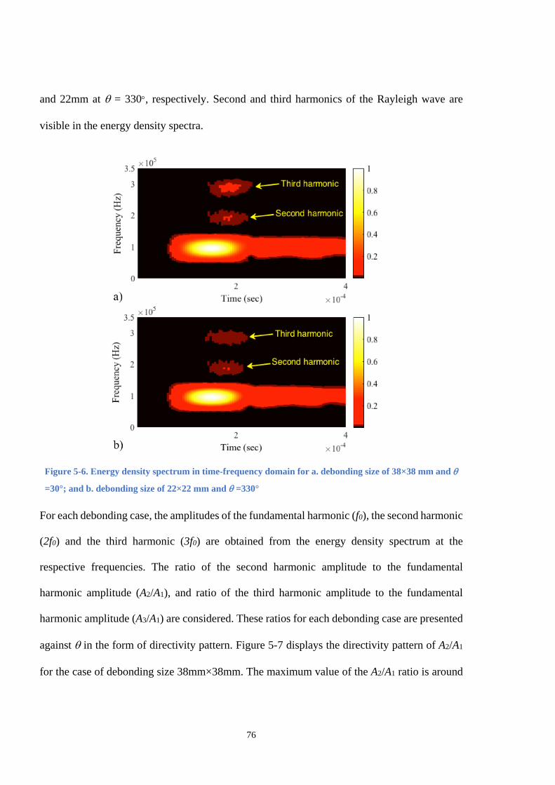
76
and 22mm at θ = 330°, respectively. Second and third harmonics of the Rayleigh wave are
visible in the energy density spectra.
Figure 5-6. Energy density spectrum in time-frequency domain for a. debonding size of 38×38 mm and θ
=30°; and b. debonding size of 22×22 mm and θ =330°
For each debonding case, the amplitudes of the fundamental harmonic (f0), the second harmonic
(2f0) and the third harmonic (3f0) are obtained from the energy density spectrum at the
respective frequencies. The ratio of the second harmonic amplitude to the fundamental
harmonic amplitude (A2/A1), and ratio of the third harmonic amplitude to the fundamental
harmonic amplitude (A3/A1) are considered. These ratios for each debonding case are presented
against θ in the form of directivity pattern. Figure 5-7 displays the directivity pattern of A2/A1
for the case of debonding size 38mm×38mm. The maximum value of the A2/A1 ratio is around

77
0.08, which occurs at θ = 0°. As shown in Figure 5-7, the scattering energy is mainly
concentrated in the forward scattering direction. The directivity pattern of A3/A1 for the case of
debonding size 22mm×22mm is shown in Figure 5-8. As shown in Figure 5-8, the energy in
the forward scattering direction is larger than that in the backward scattering direction. The
maximum value of the A3/A1 is around 0.03 and occurs at θ = 30° and θ = 330°.
Figure 5-7. Directivity pattern for second harmonic amplitude to fundamental harmonic amplitude ratio
(A2/A1) in the model with debonding size 38mm × 38mm
Figure 5-8. Directivity pattern for third harmonic amplitude to fundamental harmonic amplitude ratio
(A3/A1) in the model with debonding size 22mm × 22mm
0.02
0.04 0.06 0.08
30
210
60
240
90
270
120
300
150
330
180 0
Debondingcentre
Incidentwave
0.01
0.02
0.03
30
210
60
240
90
270
120
300
150
330
180 0
Debondingcentre
Incidentwave

78
Figures 5-9 to 5-12 show the higher harmonic amplitudes of Rayleigh wave with respect to
RDW at different directions. Figure 5-9 shows the A2/A1 ratio in the forward scattering direction
as a function of RDW. At θ = 0°, the A2/A1 ratio starts with a rapid rise and a then a sharp drop
until RDW =1. After that, it increases constantly to a peak of 0.0864 at RDW = 2. At θ = 30° and
θ = 330°, the A2/A1 ratio first increases sharply to a peak of 0.0683 and then decreases steeply
to 0.0343 at RDW = 1. It then shows some fluctuations with a decreasing trend. The A2/A1 ratio
at θ = 60° and θ = 300° drops slowly until RDW = 1, and then exhibits moderate fluctuations. At
θ = 90° and θ = 270°, the A2/A1 ratio rises gradually to 0.0480 until RDW =1, it then falls to
0.0334 at RDW =1.36. After this point, it increases slowly to 0.0363 at RDW = 2.
Figure 5-9. Second harmonic amplitude to fundamental harmonic amplitude ratio (A2/A1) in the forward
scattering direction as a function of debonding size to wavelength ratio
Figure 5-10 shows the A3/A1 ratio in the forward scattering direction as a function of RDW.
At θ = 0°, the A3/A1 ratio begins with a sudden rise, next a sharp drop, and then a steep increase
to a peak of 0.0420 at RDW = 1.36. Then, it decreases slowly to 0.0375 at RDW = 2. At θ = 30°
and θ = 330°, the A3/A1 ratio first increases rapidly to 0.0335 and then falls gradually to 0.0229
at RDW = 1.36. Then, it increases steadily to a peak of 0.0416 at RDW = 1.73. The A3/A1 ratio at
0.5 1 1.5 20
0.05
0.1
Debonding size to wavelength ratio
Seco
nd to
fund
amen
tal h
arm
onic
ratio
θ=90o
θ=60o
θ=30o
θ=0o
θ=330o
θ=300o
θ=270o

79
θ = 60°, θ = 300°, θ = 90° and θ = 270° is notably smaller than amplitude ratio at θ = 0°, θ =
30° and θ = 330° while exhibiting moderate fluctuations.
The A2/A1 ratio in the backward scattering direction as a function of RDW is shown in Figure
5-11. The A2/A1 ratios at θ = 120°, θ = 240°, θ = 150°, θ = 210° and θ = 180° show slight
fluctuations. As shown in Figure 5-11, the A2/A1 ratio at θ = 150°, θ = 210° and θ = 180° is
slightly bigger than that at θ = 120° and θ = 240°. Figure 5-12 displays the A3/A1 ratio in the
backward scattering direction as a function of RDW. At θ = 150°, θ = 210° and θ = 180°, it is
obvious that the A3/A1 ratio in the backward scattering direction is markedly smaller than that
of A2/A1 ratio and it fluctuates around 0.006-0.009. However, at θ = 120° and θ = 240°, the
amplitude starts with small values and slight fluctuations until RDW = 1.36. After that, it
increases steadily to a peak of 0.0024, and then falls steeply to 0.0062 at RDW = 2.
Figure 5-10. Third harmonic amplitude to fundamental harmonic amplitude ratio (A3/A1) in the
forward scattering direction as a function of debonding size to wavelength ratio
0.5 1 1.5 20
0.05
0.1
Debonding size to wavelength ratio
Third
to
fund
amen
tal h
arm
onic
ratio
θ=90o
θ=60o
θ=30o
θ=0o
θ=330o
θ=300o
θ=270o

80
Figure 5-11. Second harmonic amplitude to fundamental harmonic amplitude ratio (A2/A1) in the
backward scattering direction as a function of debonding size to wavelength ratio
Figure 5-12. Third harmonic amplitude to fundamental harmonic amplitude ratio (A3/A1) in backward
scattering direction as a function of debonding size to wavelength ratio
The overall trends of the second harmonic and third harmonic of the Rayleigh wave in the
forward and backward scattering direction are discussed for the cases of rectangular
debondings. For smaller values of RDW, the A2/A1 ratio has larger values at θ = 30° and θ = 330°
than θ = 0°. However, for RDW >1.36, the largest values of A2/A1 ratio are at θ = 0°. The
maximum values of A3/A1 ratio in the forward scattering direction occur at θ = 0°, and then at
θ = 30° and θ = 330°. In general, the second and third harmonics in backward scattering
0.5 1 1.5 20
0.05
0.1
Debonding size to wavelength ratio
Seco
nd to
fund
amen
tal h
arm
onic
ratio
θ=90o
θ=120o
θ=150o
θ=180o
θ=210o
θ=240o
θ=270o
0.5 1 1.5 20
0.05
0.1
Debonding size to wavelength ratio
Third
to fu
ndam
enta
l har
mon
ic ra
tio
θ=90o
θ=120o
θ=150o
θ=180o
θ=210o
θ=240o
θ=270o

81
direction have smaller amplitudes than that in the forward scattering direction. Besides, it is
obvious that the third harmonic in the backward scattering direction are smaller than that of
second harmonic for cases of rectangular debondings.

82
6 Debonding localisation in FRP-retrofitted concrete based on
scattering of linear Rayleigh wave
This chapter investigates the application of linear Rayleigh wave for detecting debonding in
FRP-retrofitted concrete structures. A method based on Time-of-flight (ToF) is developed to
locate debonding between the FRP and concrete. A 3D FE model is used to simulate the
Rayleigh wave propagation and scattering at the debonding in the FRP-retrofitted concrete
structure. A series of numerical case studies are carried out to demonstrate the capability of
the proposed debonding detection method. Different debonding sizes and locations are
considered in the case studies. It is demonstrated that the ToF-based method is capable of
locating debonding at FRP/concrete interface.
6.1 Basics of debonding localisation method
ToF is an important feature of a guided wave signal in time domain. ToF-based damage
localization has been widely used in guided wave damage detection [125-128]. Basically, ToF
can be defined as the time difference between the incident wave and damage-scattered wave,
actuated and captured by the same pair of actuator-sensor. Considering FRP-retrofitted
concrete model with debonding between FRP and concrete, the simplest case is when
debonding is located exactly on the projection of actuator and sensor connection. First, the
sensor captures the incident wave. Then, wave propagates and reflects back from debonding,
which is captured again by the sensor as shown in Figure 6-1. Difference of ToF of debonding-
scattered wave and that of incident wave (∆t) and the group velocity of the wave (Cg) can be
used to locate the debonding:

83
𝐿𝐿 =12�𝐶𝐶𝑔𝑔.∆𝑡𝑡� (32)
Figure 6-1. Schematic diagram of 1D damage localization in FRP-retrofitted concrete using ToF
Figure 6-2 illustrates an FRP-retrofitted concrete element with a pair of actuator-sensor
attached on FRP composite. Actuator, sensor and debonding are assumed to be located at
(xA,zA), (xs,zs) and (xD,zD) respectively. Now, Equation 32 can be expanded as:
∆𝑡𝑡 = 𝑡𝑡𝐴𝐴−𝐷𝐷−𝑆𝑆 − 𝑡𝑡𝐴𝐴−𝑆𝑆
= (�(𝑥𝑥𝐷𝐷 − 𝑥𝑥𝐴𝐴)
2 + (𝑧𝑧𝐷𝐷 − 𝑧𝑧𝐴𝐴)2
𝐶𝐶𝑔𝑔+�(𝑥𝑥𝐷𝐷 − 𝑥𝑥𝑆𝑆)
2 + (𝑧𝑧𝐷𝐷 − 𝑧𝑧𝑆𝑆)2
𝐶𝐶𝑔𝑔)
−�(𝑥𝑥𝑆𝑆 − 𝑥𝑥𝐴𝐴)
2 + (𝑧𝑧𝑆𝑆 − 𝑧𝑧𝐴𝐴)2
𝐶𝐶𝑔𝑔
(33)
where Cg is the group velocity. The solution to this equation is an ellipse, presented by dotted
line, which indicates the potential locations of the damage.
Sensor Actuator
Debonding Guided waves
L
Concrete
FRP

84
In the real situation, where we have a network of transducers, each operating as both
actuator and sensor, Equation 33 can be further expanded. With a network consisting of N
transducers, this equation can be applied to each pair of transducers, transducer (i) and
transducer (j), where i, j= 1, 2,…, N and i≠ j. If ∆ti-j denotes difference between ToF of wave
generated by actuator (i), scattered by damage and then captured by sensor (j), and ToF of
wave generated by actuator (i) and captured directly by sensor (j), we can expand Equation 33
as [28]:
∆𝑡𝑡𝑖𝑖−𝑗𝑗 = (�(𝑚𝑚𝐷𝐷−𝑚𝑚𝑖𝑖)
2+(𝑧𝑧𝐷𝐷−𝑧𝑧𝑖𝑖)2
𝐶𝐶𝑔𝑔+
�(𝑚𝑚𝐷𝐷−𝑚𝑚𝑗𝑗)2+(𝑧𝑧𝐷𝐷−𝑧𝑧𝑗𝑗)
2
𝐶𝐶𝑔𝑔) −
�(𝑚𝑚𝑖𝑖−𝑚𝑚𝑗𝑗)2+(𝑧𝑧𝑖𝑖−𝑧𝑧𝑗𝑗)
2
𝐶𝐶𝑔𝑔 (34)
The solution of a set of above-mentioned equations will result in a number of elliptic shapes,
the common intersections of which, can locate the damage.
Figure 6-2. Schematic diagram of damage localization in FRP-retrofitted concrete element using a pair
of actuator/sensor
Concrete
FRP
Debonding
Actuator
Sensor
Y
X
Z

85
6.2 Numerical model description
In the FE model in this chapter, S4R shell elements are used to model the FRP laminate and
C3D8R solid elements are used to model the concrete. As discussed in Section 4.6.1, rebars in
the concrete has minor effects on the measured Rayleigh wave and only cause body wave
reflections, which could be removed by baseline subtraction. Effects of rebars on Rayleigh
wave scattering from debonding are further discussed in Section 6.3. Therefore, the rebars are
not modelled in the FE model in this chapter. In the literature, it is shown that limiting the
excitation frequency up to 150 kHz could minimise the Rayleigh wave scattered from concrete
aggregates [116]. Therefore, a 150 kHz narrow-band five-cycle sinusoidal tone bust pulse
modulated by a Hanning window is used as the excitation signal in this section. The Rayleigh
wave is generated by applying out-of-plane nodal displacement to the FE nodes covered by a
10mm diameter circular transducer area. The Rayleigh wave was measured by monitoring out-
of-plane nodal displacements. Shell elements with dimension 1mm × 1mm and solid elements
with dimension 1mm × 1mm × 1mm are used in ABAQUS models. This ensures at least 12
FE nodes exist per wavelength, and hence, guarantees the accuracy of the FE simulations. The
stable time increment is automatically controlled by ABAQUS as described in Section 3.1. To
simulate the FRP-retrofitted concrete, surface-to-surface tie constraint is applied to connect
nodes between the shell and solid elements. The debonding between FRP and concrete is
simulated by untying nodes covered by the debonding area.
The Young's modulus and density of the concrete are assumed to be 25GPa and 2400kg/m3,
respectively. The FRP composite is 4-ply with layup sequence of [0/90]S. The thickness of
each lamina is 0.2mm. The fibre weight fraction; Wf; is assumed to be 0.8. Table 6-1 shows
the mechanical properties of the carbon fibre and epoxy resin.

86
Table 6-1. Elastic properties of carbon fibre and epoxy resin
Elastic properties of carbon fibre Ef11
(GPa) Ef22
(GPa) Gf12
(GPa) Gf23
(GPa) ρf
(kg/m3) νf12
231 14.48 22.75 4.83 1760 0.27
Elastic properties of epoxy matrix Em
(GPa) Gm
(GPa) ρm
(kg/m3) νm
3.77 1.35 1220 0.40
Chamis [129] formulated mechanical properties of a composite ply based on the properties
of fibre and matrix as:
𝜌𝜌 = 𝑉𝑉𝑓𝑓𝜌𝜌𝑓𝑓 + 𝑉𝑉𝑚𝑚𝜌𝜌𝑚𝑚 (35)
𝐸𝐸11 = 𝑉𝑉𝑓𝑓𝐸𝐸𝑓𝑓11 + 𝑉𝑉𝑚𝑚𝐸𝐸𝑚𝑚 (36)
𝐸𝐸22 = 𝐸𝐸33 =𝐸𝐸𝑚𝑚
1 −�𝑉𝑉𝑓𝑓(1 − 𝐸𝐸𝑚𝑚𝐸𝐸𝑓𝑓22
)
(37)
𝐺𝐺12 = 𝐺𝐺13 =𝐺𝐺𝑚𝑚
1 −�𝑉𝑉𝑓𝑓(1 − 𝐺𝐺𝑚𝑚𝐺𝐺𝑓𝑓12
)
(38)
𝐺𝐺23 =𝐺𝐺𝑚𝑚
1 −�𝑉𝑉𝑓𝑓(1 − 𝐺𝐺𝑚𝑚𝐺𝐺𝑓𝑓23
)
(39)
𝜈𝜈12 = 𝜈𝜈13 = 𝑉𝑉𝑓𝑓𝜈𝜈𝑓𝑓12 + 𝑉𝑉𝑚𝑚𝜈𝜈𝑚𝑚 (40)
𝜈𝜈23 =𝐸𝐸22
2𝐺𝐺23− 1 (41)
where V, W, E, G, ρ and ν represent the volume fraction, weight fraction, modulus of elasticity,
shear modulus, density and Poisson's ratio of constituent materials, respectively. Also, the

87
subscripts f and m denote the properties of fibre and matrix. Based on the elastic properties of
carbon fibre and epoxy matrix, and carbon fibre weight fraction, the elastic properties of each
FRP lamina are shown in Table 6-2.
Table 6-2. Mechanical properties of each FRP ply
E11 (GPa)
E22 (GPa)
E33 (GPa)
G12 (GPa)
G13 (GPa)
G23 (GPa) ν12 ν13 ν23
ρ (kg/m3)
170.78 10.30 10.30 6.97 6.97 3.53 0.30 0.30 0.46 1617
6.3 Numerical case studies
To validate the ToF-based damage localisation explained in Section 6.1, a series of numerical
case studies are considered. In the numerical case studies, the dimensions of the 4-ply FRP are
250mm × 200mm, which is bonded to a 250mm × 200mm × 80mm (L×W×H) concrete. 40mm
wide ALIDs are applied to the boundaries of FRP and concrete parts. ALID is consisted of 40
layers; each 1mm thick; which is equal to the element size. Considering Equation 28, P was
set to 3 and αmax was 2.5×10⁶. The assembly of FRP/concrete model is shown in Figure 6-3.
Four cases are considered in the numerical case studies. Cases 1–3 consider a 6mm diameter
circular debonding located at three different locations as shown in Figure 6-4. Based on the
Cartesian coordinate shown in Fig. 46, the coordinates of the PZT and the centres of the
debondings are summarised in Tables 6-3 and 6-4, respectively. Case 4 considers a debonding
at the same location as Case 3 but the diameter of the debonding is increased to 8mm.

88
Figure 6-3. FE model of FRP-retrofitted concrete
Figure 6-4. PZT and debonding locations in Cases 1-3 of the numerical studies
In each case, Rayleigh wave is sequentially generated by each PZT, and at the same time the
wave signals are measured by the rest of the PZTs. A model without the debonding is used for
baseline subtracting purpose to extract the scattered wave signal. The scattered wave is obtained
by subtracting the simulated displacement responses of the model with debonding from those
of the intact model. Rayleigh wave signals are normalised based on the maximum absolute
amplitude of signal in the model without debonding. Figure 6-5a shows the incident wave
generated by PZT-1 and captured at PZT-3 in the model without debonding in Case 4. Figure
6-5b presents wave generated by PZT-1, scattered at the debonding and then captured by PZT-
3. The scattered signal is shown in Figure 6-5c.

89
(a)
(b)
(c)
Figure 6-5. Wave signals generated by PZT-1 and captured by PZT-3 in the model without rebars a. signal
from model without debonding; b. signal from model with debonding; and c. scattered signal obtained from
baseline subtraction
0 1 2x 10⁻⁴
-1
-0.5
0
0.5
1
Time (sec)
Nor
mal
ised
Am
plitu
de
Incident wave
0 1 2x 10⁻⁴
-1
-0.5
0
0.5
1
Time (sec)
Nor
mal
ised
Am
plitu
de
Incident wave Scattering fromdebonding
0 1 2x 10⁻⁴
-0.1
0
0.1
Time (sec)
Nor
mal
ised
Am
plitu
de

90
As discussed in Section 4.6.1, rebars have minor effects on incident Rayleigh waves and
rebar reflections can be removed by the baseline subtraction. To demonstrate the effect of rebar
in wave propagation, 10mm diameter steel bars with a concrete cover of 50mm are added to the
FE model. Figure 6-6a displays the incident wave generated by PZT-1 and captured at PZT-3
in the model with rebar and without debonding between FRP and concrete. Figure 6-6b shows
the wave signal generated by PZT-1, scattered at the debonding and then captured by PZT-3.
The scattered signal from debonding in the model with rebars is shown in Figure 6-6c. As
demonstrated in Figures 6-5c and 6-6c, the scattered signal is the same for both models, i.e.
without and with rebars.
Table 6-3. Coordinates of the PZT centres in numerical case studies
PZT x (mm) z (mm) 1 50 150 2 50 50 3 200 50 4 200 150
Table 6-4. Coordinates of the debonding centres and diameters in numerical case studies
Case x (mm) z (mm) Debonding diameter (mm) 1 80 120 6 2 125 80 6 3 225 80 6 4 225 80 8
It should be noted that experimentally measured Rayleigh wave signals contain some
degrees of noise. The quality of signals can be improved significantly by averaging and also
applying a bandpass filter. Thus, for all numerical case studies of damage localisation, 2% of
noise was added to the signals obtained from FE simulations. That could ensure that the
proposed method can be used in practical situations. Figure 6-7 shows the signal generated by
PZT-4 and captured by PZT-3 for debonding Case 4 with the added noise.

91
(a)
(b)
(c)
Figure 6-6. Wave signals generated by PZT-1 and captured by PZT-3 in the model with rebars a. signal
from model without debonding; b. signal from model with debonding; and c. scattered signal obtained from
baseline subtraction
0 1 2x 10⁻⁴
-1
-0.5
0
0.5
1
Time (sec)
Nor
mal
ised
Am
plitu
de
Incident wave
Rebarreflections
0 1 2x 10⁻⁴
-1
-0.5
0
0.5
1
Time (sec)
Nor
mal
ised
Am
plitu
de
Incident wave Scattering fromdebonding
Rebarreflections
0 1 2x 10⁻⁴
-0.1
0
0.1
Time (sec)
Nor
mal
ised
Am
plitu
de

92
Figure 6-7. Wave signals generated by PZT-4 and captured by PZT-3 for debonding Case 4
The ToF is calculated based on the difference of arrival time of incident wave and the
scattered wave from the debonding. Elliptic solutions of Cases 1–3 are obtained based on
Equation 36 for each debonding location and are shown in Figures 6-8a to 6-8c, respectively.
The intersection of each pair of ellipses is indicated by a solid circle. The area with the highest
concentration of circles, as indicated by an ellipse with red dotted line, is the most probable
location of the debonding. The true debonding location and size are indicated by circles with
solid blue line.
(a)
0 1 2x 10⁻⁴
-1
-0.5
0
0.5
1
Time (sec)
Nor
mal
ised
Am
plitu
de
0 50 100 150 200 250
0
50
100
150
200
x (mm)
z (m
m)
Estimated locationof debonding
PZT-3PZT-2
PZT-1 PZT-4
True location ofdebonding

93
(b)
(c)
Figure 6-8. Elliptic solutions for 6mm diameter circular debonding in a. Case 1; b. Case 2; and c. Case 3
To validate the proposed ToF-based damage localisation method for larger size of
debonding, Case 4 considers an 8mm diameter circular debonding located at the same location
as the debonding in Case 3. The elliptic solution for this case is shown in Figure 6-9.
Figure 6-9. Elliptic solutions for 8mm diameter circular debonding in Case 4
0 50 100 150 200 250
0
50
100
150
200
x (mm)z
(mm
)
PZT-2 PZT-3
PZT-4PZT-1
True location ofdebonding
Estimeted locationof debonding
0 50 100 150 200 250
0
50
100
150
200
x (mm)
z (m
m)
PZT-1 PZT-4
PZT-2 PZT-3
Estimated locationof debonding
True location ofdebonding
0 50 100 150 200 250
0
50
100
150
200
x (mm)
z (m
m)
PZT-3
PZT-4PZT-1
PZT-2
Estimated locationof debonding
True locationof debonding

94
As shown in Figures 6-8 and 6-9, the ToF-based damage localisation method is successfully
applied to detect debonding at FRP/concrete interface.

95
7 Locating debonding in FRP-retrofitted concrete using nonlinear
Rayleigh wave
This chapter presents the application of nonlinear Rayleigh wave to detect debonding in CFRP-
retrofitted concrete structures. The proposed method requires a network of transducers that are
used to sequentially scan the CFRP-retrofitted reinforced concrete structures by transmitting
and receiving Rayleigh wave. The second harmonic of Rayleigh wave due to contact
nonlinearity at debonding between CFRP and concrete is used to detect debonding. A damage
image reconstruction algorithm is proposed to provide a graphical representation for detecting
and locating the debonding in the CFRP-retrofitted reinforced concrete structures. In this
chapter, experimental case studies are used to demonstrate the performance of the proposed
damage detection technique. A transducer array using four piezoelectric transducers to actuate
Rayleigh wave and measure the second harmonic wave in the experiments. The results show
that the proposed debonding detection technique is reliable in detecting and locating the
debonding in the CFRP-retrofitted reinforced concrete structures.
7.1 Debonding detection method using nonlinear Rayleigh wave
The proposed damage detection method determines the existence and location of the debonding
based on second harmonic Rayleigh wave. A transducer array with N transducers is required to
sequentially scan the targeted structures using Rayleigh wave. Each of the transducer can be
used as both actuator and sensor to excite and measure the wave signals, respectively. In the
sequential scan, one of the transducers is used to generate the Rayleigh wave in the CFRP-

96
retrofitted reinforced concrete structure, the rest of the transducers are used to measure the wave
signals. This provides a total of N(N-1) actuator/sensor signal paths.
Figure 7-1. a. Rayleigh wave propagation and scattering at debonding between CFRP and concrete
interface; and b. discretization of inspection area by image pixels
Figure 7-1a shows a transducer array with four transducers, T1, T2, T3 and T4, which is used
as an example to illustrate the proposed debonding detection method. In the sequential scan,
the transducer T1 is first used as the actuator to excite the Rayleigh wave, while the transducers
T2, T3 and T4 are used as the sensor to measure the wave signals. The incident Rayleigh wave
propagates and reaches the debonding. When the incident Rayleigh wave interacts with the
debonding, wave scattering occurs and the second harmonic of Rayleigh wave is also generated
due to the contact nonlinearity at the debonding. Therefore, the signals measured by the
transducers include the incident Rayleigh wave, the scattered waves from the debonding, which

97
contain components at fundamental and second harmonic frequency, and also the wave
reflected from the boundaries of the structure. This process is repeated N-1 times with
transducer T2, T3 and T4 being used as the actuator, respectively. Once the sequential scan
process is completed, the measured signals are post-processed to determine the debonding
location using the proposed damage detection method.
The idea of the proposed damage detection method is to discretise the inspection area into
image pixels as shown in Figure 7-1b. Without loss of generality, transducers i and j are used
as an example to illustrated the damage detection algorithm. When Rayleigh wave interacts
with the debonding, the second harmonic of Rayleigh wave is generated. Therefore, it is
assumed that the wave propagation can be separated into two stages. In the first stage, the
Rayleigh wave is generated from the transducer i at (xi,yi) and then propagate to the image pixel
at (x,y). In the second stage, it is assumed that the image pixel is considered as the potential
debonding location, and hence, the second stage considers the second harmonic of Rayleigh
wave is generated at the debonding location (the image pixel being considered) and propagates
to the transducer j at (xi,yi). Since the locations of the transducers and image pixels are known
in advance before carrying out the damage inspection, the group velocity of Rayleigh wave at
fundamental and second harmonic frequency can be obtained theoretically or measured
experimentally. The arrival time of the second harmonic Rayleigh wave can be calculated by:
𝐶𝐶𝑖𝑖𝑗𝑗(𝑥𝑥,𝑦𝑦) =�(𝑦𝑦 − 𝑦𝑦𝑖𝑖)2 + (𝑥𝑥 − 𝑥𝑥𝑖𝑖)2
𝑎𝑎𝑔𝑔,𝑓𝑓(𝜃𝜃𝑖𝑖)+�(𝑦𝑦𝑗𝑗 − 𝑦𝑦)2 + (𝑥𝑥𝑗𝑗 − 𝑥𝑥)2
𝑎𝑎𝑔𝑔,2𝑓𝑓(𝜃𝜃𝑗𝑗) (42)
where Cg,f and Cg,2f are the group velocity of the Rayleigh wave at fundamental and second
harmonic frequency, respectively. θi and θj are the Rayleigh wave propagation direction from

98
transducer i to the image pixel and from the image pixel to the transducer j. The first and second
term at the right-hand side of the Equation 42 is the arrival time of the fundamental frequency
of Rayleigh wave from the transducer i to the image pixel (x,y), and the second harmonic of
Rayleigh wave from the image pixel (x,y) to the transducer j, respectively.
Since the measured wave signal at transducer j contains both fundamental and second
harmonic of Rayleigh wave, a short-time Fourier transform (STFT) is used to extract the second
harmonic of Rayleigh wave and it is defined in Equation 20.
In the proposed method, a cross-correlation analysis between the incident pulse at
fundamental frequency input to transducer i and second harmonic of Rayleigh wave measured
at transducer j is used to determine the time shift for describing the source location of the second
harmonic of Rayleigh wave. As the second harmonic is induced due to the contact nonlinearity
at debonding, it can be used to determine the debonding location. Figure 7-2 shows a schematic
diagram of the incident wave and the measured nonlinear Rayleigh wave in the proposed
debonding detection technique. The incident Rayleigh wave only contains components excited
fundamental frequency. The incident Raleigh wave propagates and interacts with the
debonding. The second harmonic Rayleigh wave is then induced due to the contact nonlinearity
at the debonding. Therefore, the measured signal by the transducer contains components at both
excited fundamental frequency and second harmonic frequency as shown in Figure 7-2. With
the information of the incident wave components at the excited fundamental frequency and
damage information at the second harmonic frequency, the cross-correlation Cij is defined as:

99
𝐶𝐶𝑖𝑖𝑗𝑗(𝑡𝑡) = � 𝑆𝑆𝐹𝐹(𝜏𝜏,𝑓𝑓𝑐𝑐)𝑆𝑆𝑖𝑖𝑗𝑗(𝜏𝜏 + 𝑡𝑡, 2𝑓𝑓𝑐𝑐)𝑑𝑑𝜏𝜏𝑇𝑇
0 (43)
where SF is the STFT transformed incident pulse. Sij is the STFT transformed signal measured
by transducer j while transducer i is used as actuator. fc and 2fc is the central frequency of the
excitation signal and the corresponding second harmonic frequency, respectively.
In the sequential scan, there are N(N-1) actuator/sensor paths. For each actuator/sensor path,
the magnitude of a set of image pixels in the inspection area can be calculated and the magnitude
of the cross-correlation at the possible damage location has the largest value. To determine the
debonding location, the image indicating the possible debonding location can be obtained by
superimposing the power flux of all actuator/sensor path images as [130]
𝐼𝐼(𝑥𝑥, 𝑦𝑦) = ��𝜅𝜅𝑖𝑖𝑗𝑗𝐶𝐶𝑖𝑖𝑗𝑗�𝐶𝐶𝑖𝑖𝑗𝑗(𝑥𝑥, 𝑦𝑦)�2𝑁𝑁
𝑗𝑗≠𝑖𝑖
𝑁𝑁
𝑖𝑖=1
(44)
where κij is the weighting factor used to take into account the varying sensitivity of each
actuator/sensor path image. In this section, it is assumed to be uniform aperture weighting, i.e.
equals to unity.

100
Figure 7-2. Schematic diagram of the proposed damage debonding method and signal processing
7.2 Experimental studies
7.2.1 Experiment equipment setup
Concrete specimens 3 and 4 with debonding at FRP/concrete interface were used for
experimental measurements. Four 2mm thick and 10mm diameter circular PZT transducers
(Ferroperm Pz27) were used to actuate and sense Rayleigh wave on each specimen. The
transducers were bonded to the surface of the CFRP and they are located at T1 (x1 = 160mm, y1
= 70mm), T2 (x2 = 360mm, y2 = 70mm), T3 (x3 = 360mm, y3 = 220mm), and T4 (x4 = 160mm,
y4 = 220mm). The excitation signal is a 95kHz, 15-cycle sinusoidal tone burst modulated by a
Hanning window. Case 1 considers the concrete specimen 3 which has a 60mm×60mm
debonding between the CFRP and concrete interface. In Case 2, the concrete specimen 4 with
a 40mm×300mm debonding was used as shown in Figure 7-3.

101
Figure 7-3. Schematic diagram of the CRFP-retrofitted concrete block and the layout of the surface-
mounted transducer array (top view) a. concrete specimen 3 with 60mm×60mm debonding; and b.
concrete specimen 4 with 40mm×300mm debonding
Figure 7-4. Experiment setup for one of the scanning processes in the sequential scan
Figure 7-4 shows the experimental setup used in this study. A PC-controlled NI PXI-5412
waveform generator was used to generate the excitation signal. The amplitude of the generated
signal was then amplified by five times to 50V (peak-to-peak) using a KROHN-HITE 7500
amplifier. The Rayleigh wave signals measured by the PZT transducers and were recorded by
NI PXI-5105 digitizer and the data was then sent to computer for analysis. The sampling

102
frequency was set to 10.24 MHz and the signals were averaged 5000 times to improve the
signal-to-noise ratio.
7.2.2 Results and discussion
Figure 7-5 shows the data measured from signal path T1-T4 for the specimen in Case 1, in which
the transducer T1 is used as actuator to excite Rayleigh wave while the transducer T4 is used as
sensor to measure the scattered wave signals. It is used as an example to illustrate and explain
the wave packages in the measured signal. As mentioned in Section 7.1, the specimen has a
60mm×60mm debonding. As shown in Figure 7-5, the signal contains a number of wave
packages. The first wave package is the incident wave, which propagates directly from the
transducer T1 to T4. The second wave package is the scattered wave from the debonding. As
shown in Figure 7-3a, signal path from the transducer T1 to the debonding, and then transducer
T4 is longer than the direct signal path from the transducer T1 to T4. Therefore, the scattered
wave arrives after the incident wave. The last wave package is the waves reflected from the
boundaries and they are overlapped together as shown in Figure 7-5.
Figure 7-5. Measured data of signal path T1-T4 with debonding size 60mm × 60mm

103
Figure 7-6. Energy density spectrum in time-frequency domain for the data of signal path T1-T4 with
debonding size 60mm × 60mm
Figure 7-7. Normalised spectral amplitude of signal path T1-T4 at fundamental frequency and second
harmonic frequency for debonding size 60mm × 60mm
As shown in Figure 7-5, the scattered wave package is partially mixed with the incident
wave and boundary reflections. For damage detection technique based on the linear feature, it
is essential to extract the scattered wave signal for damage detection using baseline data.
Different to the linear feature, the second harmonic Rayleigh wave can be extracted using the
time-frequency analysis without the baseline data. Figure 7-6 shows the corresponding time-
frequency energy spectrum of the signal transformed using the STFT described in Section 7.1.

104
The figure shows that the time-frequency spectrum contains not only the signal components at
the excited fundamental frequency (95kHz), but also the second harmonic frequency (190kHz).
Figure 7-7 also shows the corresponding normalised spectral amplitude at the excited
fundamental frequency and second harmonic frequency. The second harmonic wave is
generated due to the contact nonlinearity at the debonding. When the incident wave reaches and
interacts with the debonding, the second harmonic wave is generated due to the contact
nonlinearity. The second harmonic wave propagates and is then measured by the transducer T4.
The results show that the arrival time is consistent with the scattered wave from the debonding.
Since the second harmonic wave exists at the second harmonic frequency, it does not require
the baseline data to extract the damage information.
As the specimen is the CFRP-retrofitted reinforced concrete structure, in which the CFRP is
anisotropic material while the concrete can be considered as isotropic material, the group
velocity is different in each propagation direction. Figure 7-8 shows the angular dependence of
the measured group velocity for Rayleigh wave propagation in different directions on the
CFRP-retrofitted reinforced concrete structure. The measured group velocity is used in the
proposed damage detection technique to detect and locate the debonding.

105
Figure 7-8. Angular dependence of group velocity in m/s for the CFRP-retrofitted concrete
Once the sequential scan process is completed, the measured signals are then processed using
the STFT to extract the spectral amplitude at the second harmonic frequency. Using the data
obtained at from signal path T1-T4 as an example, it is S14(t,190kHz). With this information and
the spectral amplitude of the incident wave at the excited fundamental frequency SF(t,95kHz),
an actuator/sensor path image for T1-T4 is obtained and shown in Figure 7-9. The image
indicates the feasible debonding location based on the data measured by signal path T1-T4. The
white dashed lines in the figure indicate the actual debonding location, size and shape.
Figure 7-9. Typical image of actuator/sensor signal paths T1-T4 for debonding size 60mm × 60mm
Using Equation 44, the reconstructed image for indicating the debonding location can be
obtained by superimposing all the actuator/sensor path images. Figure 7-10a shows the
reconstructed image for Case 1. Figure 7-10b shows a binary image crated from Figure 7-10a

106
by only accounting for image pixels whose intensity is larger than an arbitrary threshold value.
In this chapter, it is chosen to be 95% of the maximum intensity of the reconstructed image. In
this section, the predicted damage location is the centroid of the binary image, which is
determined as the ratio of the first- and zeroth-order spatial moments of the binary image [131].
The predicted damage location for Case 1 is at x = 0.3213m and z = 0.1710m and it is indicated
by a cross marker in Figure 7-10b.
Figure 7-10. a. Debonding location image; and b. corresponding binary image for debonding size 60mm
× 60mm (Circles: PZT transducers, dashed line: actual debonding location and size, cross: centroid of
the binary image)
Different to Case 1, Case 2 considers a debonding, which is across the whole width of the
concrete block. The reconstructed image for Case 2 is shown in Figure 7-11a and the
corresponding binary image is shown in Figure 7-11b. The same as Case 1, dashed lines are
used to indicate the actual debonding location, size and shape. The predicted damage location

107
for Case 2 is at x = 0.3188m and y = 0.1413m, and it is indicated by a cross marker in Figure 7-
11b.
Figure 7-11. a. Debonding location image; and b. corresponding binary image for debonding size 40mm
× 300mm (Circles: PZT transducers, dashed line: actual debonding location and size)
Overall, the predicted debonding locations for Cases 1 and 2 are within the actual debonding
region. The results demonstrate that the proposed damage detection technique is able to provide
a reliable prediction of the debonding location in the CFRP-retrofitted reinforced concrete
structures.

108
8 Conclusions and suggestions for future research
8.1 Conclusions
This thesis has presented a comprehensive study on the applications of Rayleigh wave for SHM
in FRP-retrofitted concrete structures. The 3D FE model has been developed to simulate
Rayleigh wave propagation in FRP-retrofitted concrete structures and scattering of signals at
debonding at FRP/concrete interface. The numerical results of group and phase velocity, and
of mode shapes of Rayleigh wave, have been verified by analytical solutions. The analytical
solution is based on the global matrix method. To experimentally validate the numerical results
of Rayleigh wave propagation and scattering, FRP-retrofitted concrete specimens have been
prepared. As discussed in Chapter 4, experimental measurements have been carried out on test
specimens to validate numerical results of Rayleigh wave propagation in FRP-retrofitted
concrete structures. Very good agreement has been observed between numerical and
experimental results. Furthermore, the numerical results of the Rayleigh wave scattering at the
bonded mass have been verified by experimental measurements. By analytical and
experimental validation of the numerical results, it has been shown that the 3D FE model can
accurately simulate the propagation and scattering of Rayleigh wave in FRP-retrofitted concrete
structures.
The scattering directivity patterns of linear Rayleigh wave at debonding at FRP/concrete
interface have also been investigated in Chapter 4. Absorbing layers by increasing damping
have been developed and applied to the numerical model in order to improve computational
efficiency of scattering analyses. Different sizes and shapes of debonding have been considered
for linear scattering studies. Scattering results have been presented in terms of RDW which is

109
defined as debonding size/diameter to the wavelength ratio. For small values of RDW,
magnitudes of forward and backward scattering are close. For larger values of RDW, the forward
scattering is more sensitive to debonding than backward scattering, demonstrating larger
magnitudes and a less complicated directivity pattern. It has been shown that the forward
scattering for rectangular and circular debonding follows a similar trend while rectangular
debonding demonstrates slightly larger magnitudes. Rectangular debondings cause larger
backward scattering than do circular debondings; however, the trend of backward scattering is
complex for both debonding shapes.
Nonlinear Rayleigh wave and higher harmonics generation of Rayleigh wave at the
debondings in FRP-retrofitted concrete structures, have been investigated in Chapter 5. The
numerical results of Rayleigh wave propagation and scattering have been presented in time,
frequency and time-frequency domains. Both second and third harmonics of Rayleigh wave,
induced by the debonding at FRP and concrete interface, have been studied in detail. Very good
agreement has been observed between numerically calculated and experimentally measured
results. It has been shown that the 3D FE model is capable of simulating nonlinear Rayleigh
wave and higher harmonic generation at the debondings. The experimentally validated 3D FE
model has been used in the parametric case studies.
To investigate scattering directivity of nonlinear Rayleigh wave, different sizes of debonding
have been considered in Chapter 5. Second and third harmonics in the forward and backward
scattering directions have been studied. The second and third harmonic amplitudes have been
presented in terms of RDW. For rectangular debondings, the amplitude of the second harmonic
is generally larger than that of the third harmonic. Also, the second and third harmonic

110
amplitudes in the forward scattering direction are larger than that in the backward scattering
direction. That means that the second and third harmonic energy is mainly concentrated in
forward scattering direction.
Scattering of linear Rayleigh wave has been used to locate debonding in FRP-retrofitted
concrete structures in Chapter 6. The proposed method is based on ToF of the incident wave
generated by actuator and directly captured by a sensor, and ToF of the wave scattered by
debonding at FRP/concrete interface. The 3D FE model has been used to simulate Rayleigh
wave propagation and scattering. Numerical case studies have been presented for different
locations and sizes of debonding. It has been demonstrated that the proposed ToF-based method
can accurately locate debonding at FRP/concrete interface in FRP-retrofitted concrete
structures.
A reference-free debonding detection technique for FRP-retrofitted concrete structures has
been presented in Chapter 7. The technique is based on nonlinear Rayleigh wave and second
harmonic generated due to contact nonlinearity at the debonding. In this chapter, the proposed
debonding detection technique has been verified using experimental results. The results show
that the reconstructed binary damage image is able to accurately predict the debonding location.
One of the advantages of the proposed debonding detection technique is that it only requires a
few transducers to locate the debonding within a reasonable size of inspection area. The
proposed technique only involves computationally efficient algorithms, such as signal
processing using STFT, and simple cross-correlation analyses. The technique can be practically
implemented using a multiplexed data acquisition system, which allows sequential excitation
of Rayleigh wave at each transducer and simultaneous measurement of signals from different

111
transducers. Therefore, the proposed imaging technique has the potential to achieve real-time
in-situ debonding detection.
Overall, this PhD research has provided physical insights into propagation of Rayleigh wave
in FRP-retrofitted concrete structures and scattering of signals at debondings at FRP/concrete
interface. It has been demonstrated that Rayleigh wave signals are sensitive to debonding
between FRP and concrete; therefore, scattering characteristics of Rayleigh wave can be used
to identify the debonding. The introduced ToF-based method proves accurate to locate the
debonding using scattering of linear Rayleigh wave. Besides, the proposed reference-free
damage localisation technique can facilitate practical applications of nonlinear Rayleigh wave
for SHM in FRP-retrofitted concrete structures.

112
8.2 Suggestions for further research
The current PhD thesis has thoroughly investigated the applications of Rayleigh wave in FRP-
retrofitted concrete structures. The following topics are suggested for further research:
• The current research has explored applications of linear and nonlinear Rayleigh waves
in FRP-retrofitted concrete structures to detect and locate debonding at FRP/concrete
interface. However, debonding size should be defined as well. Therefore, determination
of size/severity of debonding in FRP-retrofitted concrete structures can be considered
for future studies.
• In this research, the debonding in experimental specimens was created by using Mylar
sheet. For future studies, generation of real debonding conditions in test specimens can
be considered.
• In addition to debonding at FRP/concrete interface, delamination inside FRP composite
can be considered. In this regard, different combinations of debonding/delamination can
be investigated. For instance, various cases of delamination; e.g. different orientations
can be studied.
• FRP composites are not only applied on concrete structures and can be used to retrofit
different types of structures. For those cases, debonding between FRP and the substrate
can be investigated.
• In this research, only CFRP composites have been considered in numerical simulations
and experimental measurements. It is suggested that other types of FRPs be considered
for investigation.

113
9 References
[1] Worden K, Farrar CR, Manson G and Park G. The fundamental axioms of structural health
monitoring. The Royal Society A 2007; 463: 1639-1664.
[2] Rosalie C, Chan A, Chiu WK, Galea SC, Rose F and Rajic N. Structural health monitoring of
composite structures using stress wave methods. Composite Structures 2005; 67: 157-166.
[3] Heslehurst RB. Defects and damage in composite materials and structures. Boca Raton, FL, USA:
CRC Press, 2014.
[4] Sundararaman S. Static damage phenomena and models. In: Boller C, Chang F-K and Fujino Y (eds)
Encyclopedia of structural health monitoring. John Wiley and Sons, 2009.
[5] Wenzel H. Health monitoring of bridges. Chichester, UK: John Wiley and Sons, 2009.
[6] Ostachowicz W, Kudela P, Krawczuk M and Zak A. Guided waves in structures for SHM : the time-
domain spectral element method. Chichester, United Kingdom: John Wiley and Sons, 2012.
[7] Gianneo A, Carboni M and Giglio M. Feasibility study of a multi-parameter probability of detection
formulation for a Lamb waves–based structural health monitoring approach to light alloy aeronautical
plates. Structural Health Monitoring 2017; 16: 225-249.
[8] Bijudas CR, Mitra M and Mujumdar PM. Time reversed Lamb wave for damage detection in a
stiffened aluminum plate. Smart Materials and Structures 2013; 22: 1-8.
[9] Zhang B, Sun XC, Eaton MJ, Marks R, Clarke A, Featherston CA, Kawashita LF and Hallett SR.
An integrated numerical model for investigating guided waves in impact-damaged composite laminates.
Composite Structures 2017; 176: 945-960.
[10] Tian Z, Yu L and Leckey C. Delamination detection and quantification on laminated composite
structures with Lamb waves and wavenumber analysis. Journal of Intelligent Material Systems and
Structures 2015; 26: 1723-1738.
[11] Sherafat MH, Guitel R, Quaegebeur N, Lessard L, Hubert P and Masson P. Guided wave scattering
behavior in composite bonded assemblies. Composite Structures 2016; 136: 696-705.

114
[12] Harb MS and Yuan FG. A rapid, fully non-contact, hybrid system for generating Lamb wave
dispersion curves. Ultrasonics 2015; 61: 62-70.
[13] Rose JL. Ultrasonic guided waves in solid media. New York, NY, USA: Cambridge University
Press, 2014.
[14] Turco A, Bocciarelli M, Nanni A and Poggi C. Influence of width and thickness of composite
laminates on the flexural behavior of reinforced concrete beams and slabs. Composite Structures 2017;
178: 186-194.
[15] Shaw I and Andrawes B. Repair of damaged end regions of PC beams using externally bonded FRP
shear reinforcement. Construction and Building Materials 2017; 148: 184-194.
[16] Jiang G, Dawood M, Peters K and Rizkalla S. Global and local fiber optic sensors for health
monitoring of civil engineering infrastructure retrofit with FRP materials. Structural Health Monitoring
2010; 9: 309-314.
[17] Nassr AA and Dakhakhni WWE. Damage detection of FRP-strengthened concrete structures using
capacitance measurements. Journal of Composites for Construction 2009; 13: 486-497.
[18] Karbhari VM, Chin JW, Hunston D, Benmokrane B, Juska T, Morgan R, Lesko JJ, Sorathia U and
Reynaud D. Durability gap analysis for fiber-reinforced polymer composites in civil infrastructure.
Composites for Construction 2003; 7: 238-247.
[19] ACI-440R-07. Report on fiber-reinforced polymer (FRP) reinforcement for concrete structures.
ACI Committee 440, 2007.
[20] Karbhari VM, Kaiser H, Navada R, Ghosh K and Lee L. Methods for detecting defects in composite
rehabilitated concrete structures. Report no. SPR 336, 2005. Submitted to Oregon Department of
Transportation, and Federal Highway Administration.
[21] Kim SD, In CW, Cronin KE, Sohn H and Harries K. Reference-free NDT technique for debonding
detection in CFRP-strengthened RC structures. Journal of Structural Engineering 2007; 133: 1080-
1091.

115
[22] Giurgiutiu V and Bao J. Embedded-ultrasonics structural radar for in situ structural health
monitoring of thin-wall structures. Structural Health Monitoring 2004; 3: 121-140.
[23] Clarke T and Cawley P. Enhancing the defect localization capability of a guided wave SHM system
applied to a complex structure. Structural Health Monitoring 2010; 10: 247-259.
[24] Chakraborty A. Modeling of Lamb waves in composite structures. In: Boller C, Chang F-K and
Fujino Y (eds) Encyclopedia of structural health monitoring. John Wiley and Sons, 2009.
[25] Memmolo V, Monaco E, Boffa ND, Maio L and Ricci F. Guided wave propagation and scattering
for structural health monitoring of stiffened composites. Composite Structures 2018; 184: 568-580.
[26] Lamb H. On waves in an elastic plate. Proceedings of the Royal Society of London, Series A:
Mathematical, Physical and Engineering Sciences 1917; 93: 114-128.
[27] Rayleigh L. On waves propagated along the plane surface of an elastic solid. Proceedings of the
London Mathematical Society 1889; 1: 4-11.
[28] Su Z and Ye L. Identification of damage using lamb waves: from fundamentals to applications.
Berlin: Springer, 2009.
[29] Giurgiutiu V. Structural health monitoring with piezoelectric wafer active sensors. Kidlington,
United Kingdom: Academic Press, 2014.
[30] Mitra M and Gopalakrishnan S. Guided wave based structural health monitoring: a review. Smart
Materials and Structures 2016; 25: 1-27.
[31] Youbi FE, Grondel S and Assaad J. Signal processing for damage detection using two different
array transducers. Ultrasonics 2004; 42: 803-806.
[32] Koh YL, Chiu WK and Rajic N. Effects of local stiffness changes and delamination on Lamb wave
transmission using surface-mounted piezoelectric transducers. Composite Structures 2002; 57: 437-443.
[33] Raghavan A and Cesnik CES. Review of guided-wave structural health monitoring. The Shock and
Vibration Digest 2007; 39: 91–114.

116
[34] Rose JL. A baseline and vision of ultrasonic guided wave inspection potential. Journal of Pressure
Vessel Technology 2002; 124: 273-282.
[35] Diamanti K, Hodgkinson JM and Soutis C. Detection of low-velocity impact damage in composite
plates using Lamb waves. Structural Health Monitoring 2004; 3: 33-41.
[36] Diamanti K, Soutis C and Hodgkinson JM. Piezoelectric transducer arrangement for the inspection
of large composite structures. Composites: Part A 2007; 38: 1121-1130.
[37] Drozdz M, Moreau L, Castaings M, Lowe MJS and Cawley P. Efficient numerical modelling of
absorbing regions for boundaries of guided waves problems. AIP Conference Proceedings 2006; 820:
126-133.
[38] Rajagopal P, Drozdz M, A.Skelton E, Lowe MJS and V.Craster R. On the use of absorbing layers
to simulate the propagation of elastic waves in unbounded isotropic media using commercially available
finite element packages. NDT&E International 2012; 51: 30–40.
[39] Pettit JR, Walker A, Cawley P and Lowe MJS. A stiffness reduction method for efficient absorption
of waves at boundaries for use in commercial finite element codes. Ultrasonics 2014; 54: 1868-1879.
[40] Hosseini SMH, Duczek S and Gabbert U. Non-reflecting boundary condition for Lamb wave
propagation problemsin honeycomb and CFRP plates using dashpot elements. Composites: Part B 2013;
54: 1-10.
[41] Moreau L and Castaings M. The use of an orthogonality relation for reducing the size of finite
element models for 3D guided waves scattering problems. Ultrasonics 2008; 48: 357-366.
[42] Cegla FB, Rohde A and Veidt M. Analytical prediction and experimental measurement for mode
conversion and scattering of plate wavesat non-symmetric circular blind holes in isotropic plates. Wave
Motion 2008; 45: 162-177.
[43] Ihn JB and Chang FK. Pitch-catch active sensing methods in structural health monitoring for aircraft
structures. Structural Health Monitoring 2008; 7: 5-19.

117
[44] Ng CT, Veidt M and Rajic N. Integrated piezoceramic transducers for imaging damage in
composite laminates. Proceeding of the 2nd International Conference on Smart Materials and
Nanotechnology in Engineering. China: SPIE, 2009.
[45] Vanli OA and Jung S. Statistical updating of finite element model with Lamb wave sensing data
for damage detection problems. Mechanical Systems and Signal Processing 2014; 42: 137-151.
[46] Ng CT. Bayesian model updating approach for experimental identification of damage in beams
using guided waves. Structural Health Monitoring 2014; 13: 359-373.
[47] Zhao J, Ji H and Qiu J. Modeling of Lamb waves in composites using new third-order plate theories.
Smart Materials and Structures 2014; 23.
[48] Pant S, Laliberte, Martinez M and Rocha B. Derivation and experimental validation of Lamb wave
equations for an n-layered anisotropic composite laminate. Composite Structures 2014; 111: 566-579.
[49] Hayashi T and Kawashima K. Multiple reflections of Lamb waves at a delamination. Ultrasonics
2002; 40: 193-197.
[50] Ramadas C, Balasubramaniam K, Joshi M and Krishnamurthy CV. Interaction of the primary anti-
symmetric Lamb mode (Ao) with symmetric delaminations: numerical and experimental studies. Smart
Materials and Structures 2009; 18: 1-7.
[51] Ramadas C, Balasubramaniam K, Joshi M and Krishnamurthy CV. Interaction of guided Lamb
waves with an asymmetrically located delamination in a laminated composite plate. Smart Materials
and Structures 2010; 19: 1-11.
[52] Ng CT and Veidt M. Scattering of the fundamental anti-symmetric Lamb wave at delaminations in
composite laminates. The Journal of the Acoustical Society of America 2011; 129: 1288–1296.
[53] Ng CT and Veidt M. Scattering characteristics of Lamb waves from debondings at structural
features in composite laminates. The Journal of the Acoustical Society of America 2012; 132: 115–123.

118
[54] Ng CT, Veidt M, Rose LRF and Wang CH. Analytical and finite element prediction of Lamb wave
scattering at delaminations in quasi-isotropic composite laminates. Journal of Sound and Vibration
2012; 331: 4870-4883.
[55] Peng T, Saxena A, Goebel K, Xiang Y and Liu Y. Finite element simulation of Lamb wave
propagation in damaged composite laminates and experimental validation. Adaptive Structures
Conference. National Harbor, Maryland2014.
[56] Schubert KJ, Brauner C and Herrmann AS. Non-damage-related influences on Lamb wave–based
structural health monitoring of carbon fiber–reinforced plastic structures. Structural Health Monitoring
2014; 13: 158–176.
[57] Choi E, Utui N and Kim HS. Experimental and analytical investigations on debonding of hybrid
FRPs for flexural strengthening of RC beams. Composites: Part B 2013; 45: 248–256.
[58] D’Antino T and Pellegrino C. Bond between FRP composites and concrete: Assessment of design
procedures and analytical models. Composites: Part B 2014; 60: 440-456.
[59] Perera R, Sevillano E, Arteaga A and Diego AD. Identification of intermediate debonding damage
in FRP-plated RC beams based on multi-objective particle swarm optimization without updated baseline
model. Composites: Part B 2014; 62: 205-217.
[60] Zhang SS and Teng JG. Finite element analysis of end cover separation in RC beams strengthened
in flexure with FRP. Engineering Structures 2014; 75: 550-560.
[61] Haddad RH, Al-Rousan RZ and Al-Sedyiri BK. Repair of shear-deficient and sulfate-damaged
reinforced concrete beams using FRP composites. Engineering Structures 2013; 56: 228-238.
[62] Cao VV and Ronagh HR. Reducing the seismic damage of reinforced concrete frames using FRP
confinement. Composite Structures 2014; 118: 403-415.
[63] Teng JG, Chen JF, Smith ST and Lam L. FRP-strengthened RC structures. Chichester, UK: John
Wiley and Sons, 2001.

119
[64] Pan J and Wu Y-F. Analytical modeling of bond behavior between FRP plate and concrete.
Composites: Part B 2014; 61: 17-25.
[65] Biolzi L, Ghittoni C, Fedele R and Rosati G. Experimental and theoretical issues in FRP-concrete
bonding. Construction and Building Materials 2013; 41: 182-190.
[66] Bocciarelli M and Pisani MA. Survey on the interface behaviour in reinforced concrete beams
strengthened with externally bonded FRP reinforcement. Composites: Part B 2017; 118: 169-176.
[67] Alampalli S. Effectiveness of FRP materials with alternative concrete removal strategies for
reinforced concrete bridge column wrapping. International Journal of Materials and Product
Technology 2005; 23: 338 - 347.
[68] Li Z, Leung C and Xi Y. Structural Renovation in Concrete. New York, USA: Taylor and Francis,
2009.
[69] Alampalli S and Ettouney MM. Structural health monitoring. In: Zoghi M (ed) The international
handbook of FRP composites in civil engineering. Boca Raton, FL, USA: CRC Press, 2014.
[70] Mahmoud AM, Ammara HH, Mukdadi OM, Ray I, Imani FS, Chen A and Davalos JF. Non-
destructive ultrasonic evaluation of CFRP–concrete specimens subjected to accelerated aging condition.
NDT&E International 2010; 43: 635-641.
[71] Hollaway LC. A review of the present and future utilisation of FRP composites in the civil
infrastructure with reference to their important in-service properties. Construction and Building
Materials 2010; 24: 2419–2445.
[72] Nishizaki I and Meiarashi S. Long-term deterioration of GFRP in water and moist environment.
Journal of Composites for Construction 2002; 6: 21-27.
[73] GangaRao HVS, Taly N and Vijay PV. Reinforced Concrete Design with FRP composites. Boca
Raton, FL, USA: CRC Press, 2007.

120
[74] Akuthota B, Hughes D, Zoughi R, Myers J and Nanni A. Near-field microwave detection of disbond
in carbon fiber reinforced polymer composites used for strengthening cement-based structures and
disbond repair verification. JOURNAL OF MATERIALS IN CIVIL ENGINEERING 2004; 16: 540-546.
[75] Brown JR and Hamilton HR. Quantitative infrared thermography inspection for FRP applied to
concrete using single pixel analysis. Construction and Building Materials 2013; 38: 1292-1302.
[76] ACI-440.2R-08. Guide for the design and construction of externally bonded FRP systems for
strengthening concrete structures. ACI Committee 440, 2008.
[77] Washer GA and Alampalli S. Nondestructive evaluation methods for composite materials: general
overview,visual inspection, and microwave methods. In: Zoghi M (ed) The international handbook of
FRP composites in civil engineering. Boca Raton, FL, USA: CRC Press, 2014.
[78] Tonias DE and Zhao JJ. Bridge engineering: rehabilitation, and maintenance of modern highway
bridges. New York, USA: McGraw-Hil, 2007.
[79] Ettouney MM and Alampalli S. Infrastructure health in civil engineering: application and
management. Boca Raton, FL, USA: CRC Press, 2012.
[80] Taillade F, Quiertant M, Benzarti K and Aubagnac C. Shearography and pulsed stimulated infrared
thermography applied to a nondestructive evaluation of FRP strengthening systems bonded on concrete
structures. Construction and Building Materials 2011; 25: 568-574.
[81] Feng MQ, Flaviis FD and Kim YJ. Use of microwaves for damage detection in fiber reinforced
polymer-wrapped concrete structures. Journal of Engineering Mechanics 2002; 128: 172-183.
[82] Washer GA and Alampalli S. Nondestructive evaluation methods for composite materials: infrared
thermography. In: Zoghi M (ed) The international handbook of FRP composites in civil engineering.
Boca Raton, FL, USA: CRC Press, 2014.
[83] Fam A and Mirmiran A. QA/QC, maintenance, and repair of hybrid structures. In: Zoghi M (ed)
The international handbook of FRP composites in civil engineering. Boca Raton, FL, USA: CRC Press,
2014.

121
[84] Telang NM, Dumlao C, Mehrabi AB, Ciolko AT and Gutierrez J. Field inspection of in-service
FRP bridge decks- NCHRP report 564. National Cooperative Highway Research Program 2006.
[85] Sharma A, Sharma S, Sharma S and Mukherjee A. Ultrasonic guided waves for monitoring
corrosion of FRP wrapped concrete structures. Construction and Building Materials 2015; 96: 690-702.
[86] Li J, Lu Y, Guan R and Qu W. Guided waves for debonding identification in CFRP-reinforced
concrete beams. Construction and Building Materials 2017; 131: 388-399.
[87] Washer GA and Ziehl P. Nondestructive evaluation methods for composite materials: acoustic
methods. In: Zoghi M (ed) The international handbook of FRP composites in civil engineering. Boca
Raton, FL, USA: CRC Press, 2014.
[88] Qixian L and Bungey JH. Using compression wave ultrasonic transducers to measure the velocity
of surface waves and hence determine dynamic modulus of elasticity for concrete. Construction and
Building Materials 1996; 10: 237-242.
[89] Chong KP, Carino NJ and GlennWasher. Health monitoring of civil infrastructures. Smart
Materials and Structures 2003; 12: 483-493.
[90] Hevin G, Abraham O, Pedersen HA and Campillo M. Characterisation of surface cracks with
Rayleigh waves: a numerical model. NDT&E International 1998; 31: 289-297.
[91] Edwards RS, Dixon S and Jian X. Depth gauging of defects using low frequency wideband Rayleigh
waves. Ultrasonics 2006; 44: 93-98.
[92] Sun M, Staszewski WJ, Swamy RN and Li Z. Application of low-profile piezoceramic transducers
for health monitoring of concrete structures. NDT&E International 2008; 41: 589-595.
[93] Aggelis DG and Shiotani T. Repair evaluation of concrete cracks using surface and through-
transmission wave measurements. Cement & Concrete Composites 2007; 29: 700-711.
[94] Aggelis DG, Shiotani T and Polyzos D. Characterization of surface crack depth and repair
evaluation using Rayleigh waves. Cement & Concrete Composites 2009; 31: 77-83.

122
[95] Métais V, M.Chekroun, L.LeMarrec, A.LeDuff, G.Plantier and O.Abraham. Influence of multiple
scattering in heterogeneous concrete on results of the surface wave inverse problem. NDT&E
International 2016; 79: 53-62.
[96] Lee FW, Lim KS and Chai HK. Determination and extraction of Rayleigh-waves for concrete
cracks characterization based on matched filtering of center of energy. Journal of Sound and Vibration
2016; 363: 303-315.
[97] Godinho L, Costa DDd, Areias P, Júlio E and Jr DS. Numerical study towards the use of a SH wave
ultrasonic-based strategy for crack detection in concrete structures. Engineering Structures 2013; 49:
782-791.
[98] Soleimanpour R and Ng CT. Locating delaminations in laminated composite beams using nonlinear
guided waves. Engineering Structures 2017; 131: 207-219.
[99] Rauter N, Lammering R and Kühnrich T. On the detection of fatigue damage in composites by use
of second harmonic guided waves. Composite Structures 2016; 152: 247-258.
[100] Shen Y and Cesnik CES. Modeling of nonlinear interactions between guided waves and fatigue
cracks using local interaction simulation approach. Ultrasonics 2017; 74: 106-123.
[101] He S and Ng CT. Modelling and analysis of nonlinear guided waves interaction at a breathing
crack using time-domain spectral finite element method. Smart Materials and Structures 2017; 26: 1-
15.
[102]Yelve NP, Mitra M and Mujumdar PM. Detection of delamination in composite laminates using
Lamb wave based nonlinear method. Composite Structures 2017; 159: 257-266.
[103] Soleimanpour R, Ng CT and H.Wang C. Higher harmonic generation of guided waves at
delaminations in laminated composite beams. Structural Health Monitoring 2016: 1-18.
[104] Zhang J, Xuan F-Z and Yang F. Effect of surface scratches on the characteristics of nonlinear
Rayleigh surface waves in glass. Journal of Non-Crystalline Solids 2013; 378: 101-105.

123
[105] Kawashima K, Omote R, Ito T, Fujita H and Shima T. Nonlinear acoustic response through minute
surface cracks: FEM simulation and experimentation. Ultrasonics 2002; 40: 611-615.
[106] Yuan M, Zhang J, Song SJ and Kim HJ. Numerical simulation of Rayleigh wave interaction with
surface closed cracks under external pressure. Wave Motion 2015; 57: 143-153.
[107] Shui G, Kim J-Y, Qu J, Wang Y-S and Jacobs LJ. A new technique for measuring the acoustic
nonlinearity of materials using Rayleigh waves. NDT&E International 2008; 41: 326-329.
[108] Guo S, Zhang L, Mirshekarloo MS, Chen S, Chen YF, Wong ZZ, Shen Z, Liu H and Yao K.
Method and analysis for determining yielding of titanium alloy with nonlinear Rayleigh surface waves.
Materials Science and Engineering: A 2016; 669: 41-47.
[109] Doerr C, Kim J-Y, Singh P, Wall JJ and Jacobs LJ. Evaluation of sensitization in stainless steel
304 and 304L using nonlinear Rayleigh waves. NDT&E International 2017; 88: 17-23.
[110] Chopra AK. Dynamics of structures: theory and applications to earthquake engineering. 4th ed.
Upper Saddle River, New Jersey, USA: Prentice Hall, 2012.
[111] Williams M. Structural dynamics. Boca Raton, FL, USA: CRC Press, 2016.
[112] Pavlakovic B and Lowe M. DISPERSE version 2.0.16 User's Manual. Imperial College NDT
Laboratory, 2003.
[113] Lowe MJS. Matrix techniques for modeling ultrasonic waves in multilayered media. IEEE
Transactions on Ultrasonics, Ferroelectrics, and Frequency Control 1995; 42: 525-542.
[114] Alleyne DN and Cawley P. The Interaction of Lamb Waves with Defects. IEEE transactions on
ultrasonics, ferroelectrics, and frequency control 1992; 39: 381-397.
[115] Ramadas C, Balasubramaniam K, Hood A, Joshi M and Krishnamurthy CV. Modelling of
attenuation of Lamb waves using Rayleigh damping: Numerical and experimental studies. Composite
Structures 2011; 93: 2020-2025. .
[116] Wu F and Chang F-K. Debond detection using embedded piezoelectric elements for reinforced
concrete structures – part II: analysis and algorithm. Structural Health Monitoring 2006; 5: 17-28.

124
[117] Ng CT. On accuracy of analytical modeling of Lamb wave scattering at delaminations in
multilayered isotropic plates. International Journal of Structural Stability and Dynamics 2015; 15: 1-
12.
[118] Sohn H, Park G, Wait JR, Limback NP and Farrar CR. Wavelet-based active sensing for
delamination detection in composite structures. Smart Materials and Structures 2004; 13: 153-160.
[119] Aryan P, Kotousov A, Ng CT and Cazzolato B. A model-based method for damage detection with
guided waves. Structural Control and Health Monitoring 2017; 24: 1-14.
[120] Putkis O, Dalton RP and Croxford AJ. The influence of temperature variations on ultrasonic
guided waves in anisotropic CFRP plates. Ultrasonics 2015; 60: 109-116.
[121] Aryan P, Kotousov A, Ng CT and Wildy S. Reconstruction of baseline time-trace under changing
environmental and operational conditions. Smart Materials and Structures 2016; 25: 1-10.
[122] Kim G, In C-W, Kim J-Y, Kurtis KE and Jacobs LJ. Air-coupled detection of nonlinear Rayleigh
surface waves in concrete-Application to microcracking detection. NDT&E International 2014; 67: 64-
70.
[123] Torello D, Thiele S, Matlack KH, Kim J-Y, Qu J and Jacobs LJ. Diffraction, attenuation, and
source corrections for nonlinear Rayleigh wave ultrasonic measurements. Ultrasonics 2015; 56: 417-
426.
[124] Yang Y, Ng CT, Kotousov A, Sohn H and Lim HJ. Second harmonic generation at fatigue cracks
by low-frequency Lamb waves: Experimental and numerical studies. Mechanical Systems and Signal
Processing 2018; 99: 760-773.
[125] Lemistre M and Balageas D. Structural health monitoring system based on diffracted Lamb wave
analysis by multiresolution processing. Smart Materials and Structures 2001; 10: 504-511.
[126] Kessler SS, Spearing M and Soutis C. Damage detection in composite materials using Lamb wave
methods. Smart Materials and Structures 2002; 11: 269-278.

125
[127] Harri K, Guillaume P and Vanlanduit S. On-line damage detection on a wing panel using
transmission of multisine ultrasonic waves. NDT&E International 2008; 41: 312-317.
[128] Diamanti K, Soutis C and Hodgkinson JM. Lamb waves for the non-destructive inspection of
monolithic and sandwich composite beams. Composites: Part A 2005; 36: 189–195.
[129] Chamis CC. Mechanics of composite materials: past, present and future. NASA Technical
Memorandum 100793 1984.
[130] Ng CT and Veidt M. A Lamb-wave-based technique for damage detection in composite laminates.
Smart Materials and Structures 2009; 18: 1-12.
[131] Pratt WK. Digital image processing. 2nd ed. New York, NY, USA: John Wiley and Sons, 1991.