Has The Financial System Become Safer After The Crisis?

The Changing Nature of Financial Institution Risk

Paul Calluzzo* G. Nathan Dong†

Rutgers University Columbia University

Feburary 28, 2013

ABSTRACT

Five years after the collapse of Lehman Brothers, the question of whether the U.S. financial

system has become less risky remains unanswered. On the one side, new regulations including

Dodd-Frank and Basel III have made improvement by requiring higher bank capital, and

financial institutions themselves have reduced risk-taking activities. On the other side, it has

been argued that “the fundamental risks remained and the efforts of regulators and politicians

were simply rearranging the deckchairs on the Titanic.” (Baily and Elliott 2013) This paper

highlights the changing nature of financial institution risk from 2005 to 2011. It finds that while

these institutions have become less risky individually after the crisis, the financial market has

become more vulnerable to systemic contagion. The causal inference that the crisis and the post-

crisis legislation have gradually changed the nature of financial institution risk is drawn from a

quasi-experimental design. This finding suggests that the ever more integrated financial system

might experience more synchronized contractions in future crises, providing empirical support

for the proposals of the inter-bank collective regulation of banks by Acharya (2009) in addition

to the intra-bank collective regulations as in Froot and Stein (1998) and BIS (1996, 1999).

Keywords: banking risk, financial institution, systemic risk, catastrophic risk JEL Code: G01, G20, G32

__________________________ * Dept. of Finance & Economics, Rutgers University, 1 Washington Park, Newark-New Brunswick, New Jersey 07102. E-mail: calluzzo@pegasus.rutgers.edu. † Dept. of Health, Policy & Management, Columbia University. 600 W 168th Street, New York, NY 10032, E-mail: gd2243@columbia.edu. We thank Stephen Figlewski, Jussi Keppo, Steven Kou, Felix Lopez-Iturriaga, Leonard Nakamura, Frederic Mike Scherer, Lawrence White, Liuren Wu, and participants in the 11th International Industrial Organization Conference (Boston) and 7th Annual Risk Management Conference (National University of Singapore). All errors remain our responsibility.

2

”The banking system has become safer and stronger since the financial crisis. Certain activities

that people didn't like are no longer being done.” 1

— James "Jamie" Dimon, Chairman,

President and CEO of JPMorgan Chase

I. INTRODUCTION

Nearly five years after the collapse of Lehman Brothers, the United States remains in an

uncertain period of recovery and the debate about whether its financial sector has become safer

after the 2008 financial crisis continues. Some commentators argue that new regulations

requiring higher bank capital have made improvement, and financial institutions themselves

have shifted their main business from risky investment banking and trading to safer wealth and

asset management. 2 Others argue that the fundamental banking risks remain unchanged even

after all of the efforts of regulators and politicians (Baily and Elliott 2013). While there is no

shortage of speculations and conclusions, relatively little empirical evidence has been shown to

support these arguments. This paper attempts to study the changing nature of financial

institution risk in both the traditional banking and shadow banking sectors from the boom

period before the crisis to the recovery period after the crisis.

The bankruptcies of large financial institutions including Bear Stearns and Lehman

Brothers during the recent crisis have focused considerable attention on the failure of financial

institutions and the financial system as a whole. At the firm level, regulators increased their

level of monitoring and applied stress tests to key banks. Bank managers were prompted by

regulators to assess their risk and to implement strategies that would reduce their risk. Bank

shareholders increased their scrutiny of banks and revised their investment positions, making

possible large capital gains or losses. At the market level, the financial crisis highlights the

growing importance of the shadow banking system which grew out of the securitization of

assets and the integration of banking with capital market developments. This trend has had a

profound influence on the traditional banking system and the financial system as a whole. The

importance of both traditional and shadow banking systems results from their role as providers

1“JPMorgan Chase Fails to Impress Wall Street” by Maureen Farrell, CNN Money, April 12, 2013. (Retrieved from http://money.cnn.com/2013/04/12/investing/jpmorgan-earnings/index.html) 2 “Life on Wall Street Grows Less Risky” by Aaron Lucchetti and Julie Steinberg, Wall Street Journal, September 9, 2013. (Retrieved from http://online.wsj.com/article/SB10001424127887324324404579044503704364242.html)

3

of liquidity insurance, monitoring services and information. These two banking systems are

inseparable; the regulation of each system is tied closely to the other.

The recent financial crisis has attracted considerable debate amongst academics,

politicians and the mainstream media. In part, the debate reflects a desire to understand the

factors behind the dramatic rise in banking risk in both the traditional and shadow banking

systems prior and during the crisis. However, there is also a growing recognition that financial

institutions in either system are exposed, not only, to their own risk (individual risk) but also

contribute to the risk of collapses for the entire financial system (systemic risk). 3 As a

consequence, institutions failing due to their individual risks, including both credit and

operational risk, can result in the financial market failing from contagion risk.

The link between individual institutions and contagion risk raises an interesting

question which has yet to be examined: have financial institutions become less risky or has the

financial system as a whole become less vulnerable to contagion risk after the financial crisis? In

Schumpeter’s model of creative destruction, value is created because it is competitively

profitable and survives and that which is not as profitable is destroyed. This implies that after

the crisis, not only were resources mobilized in productive directions, but high risk firms were

driven out of the marketplace and replaced by less risky firm. In this paper, we attempt to

answer this question by examining the changing nature of financial institution risk before and

after the 2008 crisis using two risk measures. The first risk measure captures the individual

institution risk using the equity losses incurred due to a low-probability, high consequence,

event such as stock price crash or bankruptcy. We call this catastrophic risk.4

Our second measure of risk gauges the contagion risk present in the market. Although

large losses in equity have been relatively rare, particularly among larger financial institutions,

recent trends towards lower capital reserves, poorer loan quality and reliance on short-term

financing makes an examination of catastrophe conditions increasingly pertinent. The

unexpected failure of even a single large financial institution, such as Bear Stearns and Lehman

Brothers, can adversely affect investors’ confidence in the banking system. To understand

3 See Chichilnisky and Wu (2006) for the theoretical foundation of collective defaults in a general equilibrium setting, and Bisias, Flood, Lo, and Valavanis (2012) for a survey of econometric measures of systemic risk. 4 In more general terms, catastrophic risks are rare events with severe natural and economic consequences, such as wars, climate changes, market crashes, and the extinction of species. They include the 2007-09 financial crisis that is a once-in-a-hundred-year event with momentous consequences for global markets, and more generally any rare event that threatens human survival, such as a large asteroid impact (Posner 2004, United Nations 2000, Chichilnisky and Eisenberger 2010).

4

contagion risk among financial institutions, we construct a risk measure that estimates the

possibility of a financial system collapses due to the failures of individual financial institutions.

The econometric measures of these two risks are VAR at 0.1% probability level and

∆CoVaR at 1% probability level (from now on defined as 1‰VaR, ∆CoVaR respectively.) Using

cross-sectional and quasi-experimental studies, we find that financial institutions have become

more robust to low-probability events from their own probability distribution, or in other

words, less risky individually. However, we find the financial market has become more

vulnerable to contagion risk after the 2007-09 financial crisis, particularly after the Bear Stearns

and Lehman Brothers bankruptcies in 2008. This finding suggests that our ever more integrated

financial market might experience more synchronized contractions in future crises. To our

knowledge, this is the first paper to examine this changing nature of banking risk for both the

traditional and shadow banking systems. An important feature of the study is the comparison

between the changes in individual and systemic risks, and the causal evidence produced by the

shock of the Bear Stearns and Lehman Brothers bankruptcies.

The actual underlying economic mechanism that caused the nature change of financial

institution risk is still up for debate. On the one hand, it could be that the new regulations have

enforced better corporate governance and more transparency; as a result, financial institutions

are less risk-taking individually (Laeven and Levine 2009). On the other hand, it could be that

the interdependence among banks that arises from financial network relationships, that were

developed for the sake of risk diversification, has made financial institutions contribute more

systemic risk to the financial system and at the same time, become more vulnerable to contagion

(Battiston, Gatti, Gallegati, Greenwald, and Stiglitz 2012).

Nonetheless, this paper provides empirical support for the proposals of the inter-bank

collective regulation of banks by Acharya (2009) in addition to the intra-bank collective

regulations as in Froot and Stein (1998) and BIS (1996, 1999). The standard theory to model the

relationship between the banks and the regulator is to consider a representative bank and its

response to regulatory mechanisms like taxes and capital requirements. 5 Such partial

equilibrium approach ignores that in general equilibrium, each bank’s investment choice has an

externality on the outcomes of other banks. Recognizing this shortcoming of representative

bank models, Acharya (2009) develops a theoretical model with multiple banks to study the

5 For literature review on banking regulation, see Dewatripont and Tirole (1993), Freixas and Rochet (1997).

5

essential properties of prudential bank regulation that takes into account both individual and

systemic bank failure risk. 6

The remainder of the paper is organized as follows. Section II reviews the relevant prior

research on individual institution risk and systemic risk. Section III presents the sample data

and measurement choice. Section IV introduces the empirical method. Section V evaluates the

results. Section VI discusses the causality concern and presents a quasi-experimental study to

address the endogeneity issue. Section VII concludes.

II. RELATED LITERATURE

This paper is closely related to the literature on catastrophic risk and operational risk of

financial institutions. Allen and Bali (2007) suggest that a bank’s operational risk is more likely

to be the cause of a large unexpected catastrophic loss than market-wide risk, although when a

loss occurs, it is smaller, on average, than those resulting from a combination of market risk,

credit risk or other risk events. They estimate catastrophic risk and operational risk using two

different methodologies: the extreme value theory, implemented using the generalized Pareto

distribution (GPD) of Pickands (1975), and a skewed fat-tailed distribution, implemented using

the skewed generalized error distribution (SGED) of Bali and Theodossiou (2008). An

interesting question arises, why is catastrophic risk relevant if investors can diversify their

portfolio holdings. One reason may be that catastrophic risk events are highly visible, even to

relatively uninformed market agents. Merton (1987) and Shapiro (2002) show that the portfolio

holdings of informationally constrained investors may be impacted by catastrophic risk event

related visibility, such that investors eschew holdings in these firms. Some regulated financial

institutions, such as banks, may have access to government-subsidized safety nets. In exchange

for these government subsidies, regulators require banks to maintain capital positions designed

to protect the overall safety and soundness of the banking system. Catastrophic risk events can

potentially cause contagion and systemic risk problems that undermine this regulatory policy

goal. Therefore, value at risk measures that focus on the lower tails of the return distribution are

important determinants of bank capital requirements.

While bank stocks plummeted during the financial crisis, the variation in the

performance amongst these banks was substantial. Some banks were much more exposed to the

6 For literature on bank contagion models, see Rochet and Tirole (1996), Kiyotaki and Moore (1997), Freixas and Parigi (1998), and Allen and Gale (2000c),

6

financial crisis than others. Studies by Flannery and Sorescu (1996), Flannery (1998), Krainer

and Lopez (2003), Furlong and Williams (2006), Distinguin, Ross, and Tarazi (2006), Curry,

Elmer, and Fissel (2007), and Curry, Fissel, and Hanweck (2008) assess whether a bank’s

financial and market data can signal information about the bank’s risk. Yet, there is very limited

research on how a bank’s financial and market data may signal information about a bank's risk

exposure during a financial crisis.

This paper is also closely related to the literature on systemic risk. The contagion effect

of an event usually refers to the spillover effects of stocks of one or more firms to others

(Kaufman 1994) but has also been characterized as the change in the value of a firm that can be

attributed to economic events with a clearer and more direct impact on some other firm

(Docking, Scott, Hirschey, and Jones 1997). Contagion has been studied widely in the theoretical

and empirical financial literature (for reviews see Flannery 1998). The focus of analysis has

ranged from strong systemic shocks involving multiple bank failures, currency crises, and

market crashes to informational spillover effects that lead to the revaluation of stock prices but

not to widespread failures. This paper contributes to the latter body of literature by analyzing

the stock price effects of operational loss events on non-announcing financial institutions. This

type of informational spillover has been analyzed extensively for other types of events. This

section discusses the prior papers with the most significant implications for the research

presented in this paper.

In order to capture systemic risk in the financial sector we use the ∆CoVaR measure

developed by Adrian and Brunnermeier (2008). ∆CoVaR is the value at risk of the entire

financial system conditional on an individual institution in distress. More formally, ∆CoVaR is

the difference between the CoVaR, conditional on a financial institution being in distress, and

the CoVaR, conditional on its operating in its median state. A number of papers have used the

∆CoVaR measure in various contexts. Brunnermeier, Dong, and Palia (2012) find that banks

actively engaged in trading, investment banking and venture capital contributed more to

systemic risk. Wong and Fong (2010) examine ∆CoVaR for credit default swaps of Asia-Pacific

banks, whereas Gauthier, Lehar and Souissi (2010) use it for Canadian institutions. Adams, Fuss

and Gropp (2010) study risk spillovers among financial institutions, including hedge funds, and

Zhou (2009) drives a CoVar measure using extreme value theory rather than quantile

regressions.

7

Recent papers have proposed complementary measures of systemic risk other than

∆CoVaR. Acharya, Pedersen, Philippon, and Richardson (2010) define Systemic Expected

Shortfall (SES) as the expected amount a bank will be undercapitalized by in a systemic event in

which the entire financial system is undercapitalized. Allen, Bali and Tang (2012) propose the

CATFIN measure, which is the principal components of the 1% VaR and expected shortfall,

using estimates of the generalized Pareto distribution, skewed generalized error distribution,

and a non-parametric distribution. Brownlees and Engle (2010) define marginal expected

shortfall (MES) as the expected loss of a bank’s equity value if the overall market declines

substantially. Tarashev, Borio, and Tsatsaronis (2010) suggest Shapley values based on a bank’s

default probability, size, and exposure to common risks could be used to assess the regulatory

taxes on each bank. Billio, Getmansky, Lo and Pelizzon (2010) use principal components

analysis, and linear and nonlinear Granger causality tests, to find the interconnectedness

between the returns of hedge funds, brokers, banks, and insurance companies. Chan-Lau (2010)

proposes the CoRisk measure, which captures the extent to which the risk of one institution

changes in response to changes in the risk of another institution, while controlling for common

risk factors. Huang, Zhou, and Zhu (2009, 2010) propose the deposit insurance premium (DIP)

measure, which is a bank’s expected loss conditional on financial system distress exceeding a

threshold level.

III. DATA

Analyzing the 1‰VaR and ∆CoVaR of financial institutions requires collecting macroeconomic

data, stock returns and financial accounting information. We focus on all publicly traded

financial institutions in the United States. Although financial institutions have similar

characteristics, they are not completely homogenous. For example, commercial banks differ

somewhat from insurance companies and from broker-dealers. We construct our sample by

searching CRSP for all firms traded on either the NYSE, AMEX or Nasdaq that had primary SIC

codes of 60 (depository institutions), 61 (non-depository institutions), 62 (brokers), 63 (insurers),

64 (insurance agents), and 67 (investments) over the time period from 2005 to 2011. To control

for differences in institution characteristics, we use market value, total asset, financial leverage,

market-to-book, maturity mismatch, stock return, volatility, and 1% Value-at-Risk. The detailed

definitions of SIC codes and control variables are shown in Table I.

[Insert Table I Here]

8

We obtain daily and monthly stock returns from CRSP which we use to convert into

weekly and annual returns. Financial statement data is from Compustat. T-Bill and LIBOR rates

are from the Federal Reserve Bank of New York and real estate market returns are from the

Federal Housing Finance Agency. There are two samples in our study: the first sample excludes

the observations in 2008 when both Bear Stearns and Lehman Brothers filed the Chapter 11. We

take the average values for each variable for the period prior to the bankruptcy (2005-2007) and

the period after the bankruptcy (2009-2011). The second sample includes the entire dataset from

2005 to 2007 and from 2009 to 2011, excluding 2008 when Bear Stearns and Lehman Brothers

filed the Chapter 11 for reorganization.

We define the catastrophic risk of the three-year daily return distribution for a financial

institution as the return in the lowest 0.1% of each of the daily observations for the period of

three years. We refer to this measure as the 1‰VaR. To measure the systemic risk for individual

institutions we use the ∆CoVaR measure developed by Adrian and Brunnermeier (2008).

∆CoVaR is the value at risk of the banking system conditional on an individual bank being in

distress. More formally, ∆CoVaR is the difference between the CoVaR, conditional on a bank

being in distress, and the CoVaR, conditional on a bank operating in its median state. We will

discuss the estimation of ∆CoVaR in the next section. The summary statistics for these two

banking risk variables and the other control variables are shown in Table II.

[Insert Table II Here]

Table III reports the Pearson’s correlations among all variables.

[Insert Table III Here]

IV. METHODOLOGY

This paper focuses on analyzing financial institution risk by estimating both 1‰VaR and

∆CoVaR, and comparing the risks between the period prior to the Bear Stearns and Lehman

bankruptcies and the period after the bankruptcies. As mentioned in the data section, we

constructed two samples: one with the 3-year averaged data prior and post 2008, and the other

one with annual data from 2005 to 2011. Both samples exclude observations in 2008 when both

9

Bear Stearns and Lehman Brother filed for Chapter 11. We apply OLS regressions with and

without clustered standard error (on industry classification) to assess the relationship between

financial institution risk and institutional characteristics and to assess the changing nature of

banking risk due to the 2007-09 financial crisis.

The most common measure of financial institutions risk, VaR (Value at Risk), focuses on

the risk of an individual institution in isolation. The q%-VaR is the maximum dollar loss within

the q%-confidence interval; see Kupiec (1998) and Jorion (2006) for overviews. In this paper, we

use the 0.1% level to capture the low probability events at the financial institutions. For an

institution, probability and time horizon, VaR is defined as a threshold value such that with

probability (q) the mark-to-market loss on the equity over the given time horizon exceeds this

value (VaR). However, a single institution’s risk measure does not necessarily reflect systemic

risk, i.e., the risk that the stability of the financial system as a whole is threatened. We use the

∆CoVaR measure of Adrian and Brunnermeier (2008) to capture this systemic risk. This measure

is one period forward and captures the marginal contribution of a financial institution to overall

systemic risk. Adrian and Brunnermeier (2008) suggest that prudential capital regulation should

not just be based on the VaRs of a bank but also on their ∆CoVaRs, which by their predictive

power alert regulators who can use them as a basis for a preemptive countercyclical capital

regulation such as a capital surcharge or Pigovian tax.

Value-at-Risk measures the worst expected loss over a specific time interval at a given

confidence level. In the context of this paper, iqVaR is defined as the percentage iR of asset

value that bank i might lose with %q probability over a pre-set horizon T :

( )i iqProbability R VaR q (1)

Thus by definition the value of VaR is generaly negative. Another way of expressing

this is that iqVaR is the %q quantile of the potential asset return in percentage term ( iR ) that

can occur to bank i during a specified time period T . The confidence level (quantile) q and the

time period T are the two major parameters in a traditional risk measure using VaR. We

consider the 1% quantile and weekly asset return/loss iR in this paper, and the VaR of bank i

is 1%( ) 1%i iProbability R VaR .

Let |system iqCoVaR denote the Value at Risk of the entire financial system (portfolio)

conditional on bank i being in distress (in other words, the loss of bank i is at its level of iqVaR ).

10

That is, |system iqCoVaR is essentially a measure of systemic risk in the q% quantile of this

conditional probability distribution:

|( | )system system i i iq qProbability R CoVaR R VaR q (2)

Similarly, let | ,system i medianqCoVaR denote the financial system’s VaR, conditional on a bank

operating in its median state (in other words, the return of bank i is at its median level). That is,

| ,system i medianqCoVaR measures the systemic risk when business is normal for bank i :

| ,( | )system system i median i iqProbability R CoVaR R median q (3)

Bank i ’s contribution to systemic risk can be defined as the difference between the

financial system’s VaR conditional on bank i in distress ( |system iqCoVaR ), and the financial

system’s VaR conditional on bank i functioning in its median state ( | ,system i medianqCoVaR ):

| | ,i system i system i medianq q qCoVaR CoVaR CoVaR (4)

To estimate this measure of a individual bank’s systemic risk contribution, i.e., iqCoVaR , we

need to calculate two conditional VaRs for each bank, namely |system iqCoVaR and

| ,system i medianqCoVaR . For the systemic risk conditional on bank in distress ( |system i

qCoVaR ), we run a

1% quantile regression using the weekly data to estimate the coefficients i , i , |system i ,

|system i and |system i :

1i i i it tR Z (5)

| | | |1 1

system system i system i system i i system it t tR Z R (6)

and run a 50% quantile (median) regression to estimate the coefficients ,i median and ,i median :

, , ,1

i i median i median i mediant tR Z (7)

where itR is the weekly growth rate of the market-valued assets of bank i at time t :

1 1

1i i

i t tt i i

t t

MV LeverageR

MV Leverage

(8)

and systemtR is the weekly growth rate of the market-valued total assets of all N banks

( 1,2,3...,i j N ) in the financial system at time t :

11

1 1

11 1

1

i i iNsystem t t tt N

j jit t

j

MV Leverage RR

MV Leverage

(9)

In equation (8) and (9), itMV is the market value of bank i ’s equity at time t , and i

tLeverage is

bank i ’s leverage defined as the ratio of its total asset and equity market value at time t :

/i i it t tLeverage Asset MV . It is noted that when we calculate the asset return of the entire

financial system in equation (9), the individual bank’s asset return is value-weighted by its total

assets, proxied by the product of equity market value (MV) and leverage at time t-1.

1tZ in equation (7) is the vector of macroeconomic and finance factors in the previous

week, including market return, equity volatility, liquidity risk, interest rate risk, term structure,

default risk and real-estate return. We obtain value-weighted market returns from the database

of the S&P 500 Index CRSP Indices Daily. We use weekly value-weighted equity returns

(excluding ADRs) with all distributions to proxy for the market return. Volatility is defined as

the standard deviation of log market returns. Liquidity risk is defined as the difference between

the three-month LIBOR rate and the three-month T-bill rate. For the next three interest rate

variables we calculate the changes from this week t to t-1. Interest rate risk is defined as the

change in the three-month T-bill rate. Term structure is defined as the change in the slope of the

yield curve (yield spread between the 10-year T-bond rate and the three-month T-bill rate.

Default risk is defined as the change in the credit spread between the 10-year BAA corporate

bonds and the 10-year T-Bond rate. All interest rate data is obtained from the U.S. Federal

Reserve website and Compustat Daily Treasury database. Real estate returns are proxied by the

Federal Housing Finance Agency’s FHFA House Price Index for all 50 U.S. states.

We predict an individual bank’s VaR and median asset return using the coefficients ˆ i ,

ˆ i , ,ˆ i median and ,ˆ i median estimated from the quantile regressions of equation (5) and (7):

, 1ˆˆ ˆi i i i

q t t tVaR R Z (10)

, , ,1

ˆˆ ˆi median i i median i mediant t tR R Z (11)

The vector of state (macroeconomic and finance) variables 1tZ is the same as in equation (5)

and (7). After obtaining the unconditional VaRs of an individual bank i ( ,iq tVaR ) and that bank’s

asset return in its median state ( ,i mediantR ) from equation (10) and (11), we predict the systemic

12

risk conditional on bank i being in distress ( |system iqCoVaR ) using the coefficients |ˆ system i , |ˆ system i ,

and |ˆ system i estimated from the quantile regression of equation (6) . Specifically,

| | | |, 1 ,

ˆˆ ˆ ˆsystem i system system i system i system i iq t t t q tCoVaR R Z VaR (12)

Similarly, we can calculate the systemic risk conditional on bank i functioning in its median

state ( | ,system i medianqCoVaR ) as:

| , | | | ,, 1

ˆˆ ˆsystem i median system i system i system i i medianq t t tCoVaR Z R (13)

Bank i ’s contribution to systemic risk is the difference between the financial system’s VaR if

bank i is at risk and the financial system’s VaR if bank i is in its median state:

| | ,, , ,

i system i system i medianq t q t q tCoVaR CoVaR CoVaR (14)

Note that this is same as equation (4) with an additional subscript t to denote the time-varying

nature of the systemic risk in the banking system. As shown in the quantile regressions of

equation (5) and (7), we are interested in the VaR at the 1% confident level, therefore the

systemic risk of individual bank at q=1% can be written as:

| | ,1%, 1%, 1%,i system i system i median

t t tCoVaR CoVaR CoVaR (15)

V. RESULTS

The summary statistics for all variables are shown in Table II, and Pearson’s correlations are

reported in Table III. Table IV provides the results of the empirical estimates for the associations

between our two risk measures and institutional characteristics.

[Insert Table IV Here]

The dependent variables are the two measures of financial institution risk: 1‰VaR and

∆CoVaR. Columns 1-2 are the 1‰VaR regressions, and columns 3-4 are the ∆CoVaR regressions.

Higher individual risk as measured by a more negative 1‰VaR is associated with more severe

maturity mismatch, higher stock return volatility, lower equity return, and lower Value-at-Risk

at 1%, whereas higher systemic risk as measured by a more negative ∆CoVaR is associated with

larger institutions (market value and total assets), more growth potentials (market-to-book), and

higher Value-at-Risk. The POSTLEHMAN dummy variable has a positive sign in the 1‰VaR

regressions but a negative sign in the ∆CoVaR regressions, suggesting that financial institutions

13

have become less sensitive to individual risk but more sensitive to systemic risk after the

bankruptcy of both Bear Stearns and Lehman Brothers in 2008. To address the concerns that

standard error clustering in certain industries within the financial sector might have biased our

coefficient estimation, we re-do our analysis using clustered standard error on industry

classification which rectifies for heteroskedasticity. The results are reported in Table V, and they

are consistent with our pervious findings.

[Insert Table V Here]

It should be recognized that the results reported in Table IV and V do not provide

further information regarding which year has the most or least significant effects. To address

this concern, we create six dummy variables with each one representing a single year from 2005

to 2011 excluding the year 2008 when Bear Stearns and Lehman Brothers filed Chapter 11.

Because we cannot include all year dummy variables in one specification, we exclude the year

2011 dummy from columns (1), (2), (5), and (6), and the year 2005 dummy from columns (3), (4),

(7) and (8). We also include the industry fixed effects for columns (2), (4), and (6), and (8). The

coefficient estimates for this analysis are shown in Table VI.

[Insert Table VI Here]

Higher individual risk as measured by a more negative 1‰VaR is associated with larger

institutions, more severe maturity mismatch, higher stock return volatility, lower equity return,

and lower Value-at-Risk at 1%. Higher systemic risk as measured by a more negative ∆CoVaR is

associated with larger institutions, lower leverage, more growth potentials, higher volatility,

and higher Value-at-Risk at 1%. The year 2009, one year after the Bear Stearns and Lehman

bankruptcies, has the most significant reduction in catastrophic risk of individual institutions

but the most significant increase in systemic risk.

Again, we re-run our analysis using clustered standard error on industry classification

to address the concerns that standard error clustering in certain industries within the financial

sector might have biased our coefficient estimations. The results are consistent with our

pervious findings as shown in Table VII.

14

[Insert Table VII Here]

VI. CAUSALITY

This paper studies the relationship between the financial crisis and its impact on the risk of the

U.S. banking sector. However, the economic interpretation of statistical significance in

correlations between the financial crisis and financial institution risks deserves caution because

the empirical results reported in the previous section do not provide “true” causal evidence as

in either Granger (1969) time-series prediction or Rubin (1974, 1978)’s causality. The above

results could be driven by endogeneity concerns. Specifically, there might be significant omitted

variable(s) correlated with both the financial crisis and financial institution risk driving our

results spuriously. To specifically address the endogeneity concern and provide Rubin causality

evidence, we need to employ a quasi-experimental study that assigns intervention (treatment)

and control (non-treatment) status to financial institutions and non-financial firms, and

examines the outcomes (changes of risk) before and after conducting the intervention or

treatment.

In this quasi-experimental study, we consider the bankruptcies of Bear Stearns and

Lehman Brothers in 2008 as an exogenous shock. We employ a difference-in-differences (DiD)

approach (see Meyer 1995, and Angrist and Krueger 1999 for detailed explanations of this

methodology). Specifically, we analyze whether the unexpected shock of Bear Stearns and

Lehman Brothers bankruptcies have changed the individual risk and the systemic risk of

financial institutions. Accordingly, financial institutions are defined as the treatment group, and

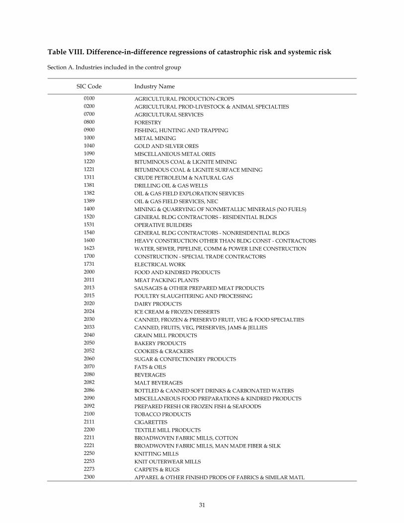
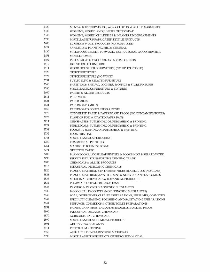
a set of non-financial firms are the control or non-treated group. See Section A of Table VIII for

the list of industries that are included in the control sample.

[Insert Table VIII Here]

The dummy variable TREATMENT is set to one for financial institutions, and zero

otherwise. The dummy variable POSTLEHMAN is set to one if the year is after the bankruptcy

event of Bear Stearns and Lehman Brothers in 2008, and zero otherwise. A third dummy

variable POSTLEHMAN×TREATMENT is the cross-product of the previous two dummy

variables. According to Meyer (1995) and Angrist and Krueger (1999), the coefficient estimate of

15

the POSTLEHMAN×TREATMENT dummy is the effect that needs to be estimated. The

coefficient estimates for this DiD analysis are shown in Section B of Table VIII. There are six

specifications in this analysis. The dependent variable in the first three specifications is 1‰VaR,

whereas the dependent variable in the rest of three specifications is ∆CoVaR. The second and

fourth specifications use industry fixed effects, and the third and sixth specifications use both

industry fixed effects and clustered standard errors. After controlling for numerous firm

characteristics and comparing financial firms to the non-financial firms, the coefficient estimates

of the interaction term (POSTLEHMAN×TREATMENT), which represents the firms in the

financial sector and the time is after the bankruptcy event, are positive for the catastrophic risk

regressions and negative for the systemic risk regressions. The DiD results from this quasi-

experimental study suggest that the bankruptcies of Bear Stearns and Lehman Brothers in 2008

have reduced the individual risk as proxied by 1‰VaR of financial firms, but increased the

systemic risk as measured by ∆CoVaR of these firms.

It should be noted that this specific quasi-experimental design can only provide causal

evidence in the sense of Rubin (1974, 1978), i.e., institutions became less risky individually but

more vulnerable to contagion risk after the exogenous shock of the bankruptcy event. However,

it has no explanation power for exactly what are the underlying economic channels that have

caused this change. It could be that the new regulations have enforced better corporate

governance and more transparency; as a result, financial institutions are less risk-taking

individually albeit contribute more systemic risk to the financial market at the same time.

Laeven and Levine (2009) suggest that there are potential conflicts between bank

managers and owners over bank risk-taking and bank regulation have different effects on bank

risk-taking depending on the comparative power of shareholders in the governance structure of

each bank. Harris and Raviv (2012) recommend two effective regulatory tools (forcing payouts

and constraining investments) that can potentially curb risk taking behavior by banks. From the

above argument, it is not difficult to infer that the post-crisis regulations might have been

successfully improved governance and reduced risk-taking in the financial sector; consequently,

financial institutions have lower level of individual risk after the financial crisis. On the other

hand, the interdependence among banks that arises from active trading7 and financial network

relationships that were developed for the sake of risk diversification might have made financial

7 Brunnermeier, Dong, and Palia (2012) find that banks actively engaged in trading, investment banking and venture capital business contributed more to systemic risk.

16

institutions contribute more systemic risk to the financial system and at the same time, become

more vulnerable to contagion (Battiston, Gatti, Gallegati, Greenwald, and Stiglitz 2012).

VII. CONCLUSION

The collapse of Lehman Brothers sparked a meltdown of the U.S. financial system in 2008. Five

years later, we are at a crucial point that calls for us to step back and examine our progress in

the effort to redesign the rules governing the financial markets. Today the United States

remains in an uncertain period of recovery and the debate about whether its financial sector has

become safer after the crisis continues. While there is no shortage of speculations and

conclusions, it does not seem possible to answer this question without providing any concrete

evidence. This paper attempts to study the changing nature of financial institution risk in both

traditional banking and shadow banking systems from the boom period before the crisis to the

recovery period after the crisis.

The recent crisis highlighted the growing importance of the shadow banking system

which grew out of the securitization of assets and the integration of banking with capital market

developments. This trend has a profound influence on the traditional banking system and the

financial system as a whole. The importance of both traditional and shadow banking systems

results from their role as providers of liquidity insurance, monitoring services and information.

These two banking systems are inseparable, and the regulations in one system are tied closely to

the regulations of the other. The bankruptcies of Bear Stearns and Lehman Brothers in 2008

have attracted considerable debate amongst academics, politicians and the mainstream media in

recent years. In part, this has reflected a desire to understand the factors behind the dramatic

rise in banking risk in both the traditional and shadow banking systems prior and during the

financial crisis. However, there is also a growing recognition that financial institutions in either

system are not only exposed to their own risk (individual risk), but they also contribute to the

risk a collapse of the entire financial system (systemic risk). As a consequence, an institution can

fail as a result of its individual risk, including both credit and operational risk, while the

financial market can fail from the contagion risk arising from the failing institutions.

In this paper, we capture the individual institution risk using the losses incurred due to

a low-probability event such as stock price crash or bankruptcy. We call this catastrophic risk.

To understand the contagion risk among financial institutions, we measure the possibilities that

the entire financial system collapses due to the failure of individual financial institutions. The

17

econometric measures of these two risks are 1‰VaR and ∆CoVaR respectively. Using cross-

sectional and quasi-experimental studies, we highlight the changing nature of banking risk, and

find financial institutions have become more robust to low-probability individual risk but the

financial market has become more vulnerable to contagion risk after (and likely caused by) the

recent crisis, particularly after the Bear Stearns and Lehman Brothers bankruptcies in 2008. This

finding suggests that our ever more integrated financial market might experience more

synchronized contractions in future crises, providing empirical support for the proposals of the

inter-bank collective regulation of banks by Acharya (2009) in addition to the intra-bank

collective regulations as in Froot and Stein (1998) and BIS (1996, 1999).

To our knowledge, this is the first study to examine this changing nature of banking risk

for both the traditional and shadow banking systems in detail. An important feature of the

study is the comparison between individual firm risk and systemic contagion risk, and the new

evidence of causal effects of the Bear Stearns-Lehman shocks on banking risk. However, we

admit that it is impossible to control for all economic and institutional factors that might affect

banking risk, and many of these factors are intrinsically difficult to quantify, or, suffer from a

lack of available data. Finally, the identification of the twin-bankruptcy shock can be weak in

the sense that our estimation of risk is annual whereas the economic impact of these bankruptcy

events can be instantaneous. This shortcoming of risk measure suggests that future research

might be directed towards the estimation of risk in a much narrower time period, i.e., daily or

weekly. We leave such issues for future research.

18

REFERENCE

Acharya, Viral, 2009, A Theory of Systemic Risk and Design of Prudential Bank Regulation, Journal of Financial Stability 5, 224–255. Acharya, Viral, Lasse Pedersen, Thomas Philippon, and Mathew Richardson, 2010, Measuring Systemic Risk, NYU Stern Working Paper. Adams, Zeno, Roland Fuss, and Reint Gropp, 2010, Modeling Spillover Effects among Financial Institutions: A State-Dependent Sensitivity Value-at-Risk (SDSVaR) Approach, EBS Working Paper. Adrian, Tobias, and Markus Brunnermeier, 2008, CoVaR, Fed Reserve Bank of New York Staff Reports. Allen, Franklin, Douglas Gale, 2000, Financial Contagion, Journal of Political Economy 108, 1–33. Allen, Linda, and Turan G. Bali, 2007, Cyclicality in Catastrophic and Operational Risk Measurements, Journal of Banking and Finance 31, 1191–1235. Allen, Linda, Turan G. Bali, and Yi Tang, 2012, Does Systemic Risk in the Financial Sector Predict Future Economic Downturns?, Review of Financial Studies 25, 3000-3036. Angrist, Joshua and Alan Krueger, 1999, Empirical Strategies in Labor Economics, Handbook of Labor Economics (Orley Ashenfelter and David Card, eds.), 3A, 1277–1366. Baily, Martin and Douglas Elliott, 2013, Five Years after Lehman, We’re Much Safer, Brookings Institution, September 9th, 2013. Bali, Turan G., and Panayiotis Theodossiou, 2008, Risk Measurement Performance of Alternative Distribution Functions, Journal of Risk and Insurance 75, 411–437. Battiston, Stefano, Domenico Delli Gatti, Mauro Gallegati, Bruce Greenwald, and Joseph E. Stiglitz, 2012, Liaisons Dangereuses: Increasing Connectivity, Risk Sharing, and Systemic Risk, Journal of Economic Dynamics and Control 36, 1121–1141. Billio, Monica, Mila Getmansky, Andrew Lo, and Loriana Pelizzon, 2010, Econometric Measures of Systemic Risk in the Finance and Insurance Sectors, NBER Paper No. 16223. BIS, 1996, Amendment to the Capital Accord to Incorporate Market Risks, Bank for International Settlements. BIS, 1999, A New Capital Adequacy Framework, Bank for International Settlements. Bisias, Dimitrios, Mark Flood, Andrew Lo, and Stavros Valavanis, 2012. A Survey of Systemic Risk Analytics, Office of Financial Research of the U.S. Department of the Treasury, Working Paper 2012–0001.

19

Brownlees, Christian, and Robert Engle, 2010, Volatility, Correlation and Tails for Systemic Risk Measurement, NYU Stern Working Paper. Brunnermeier, Markus, G. Nathan Dong, and Darius Palia, Non-interest Income and Systemic Risk, Princeton Columbia Rutgers Working Paper. Chan-Lau, Jorge, 2010, Regulatory Capital Charges for Too-Connected-to-Fail Institutions: A Practical Proposal, IMF Working Paper 10/98. Chichilnisky, Graciela, and Ho-Mou Wu, 2006, General Equilibrium with Endogenous Uncertainty and Default, Journal of Mathematical Economics 42, 499–524. Chichilnisky, Graciela, and Peter Eisenberger, 2010, Asteroids, Journal of Probability and Statistics 2010, 1–16. Curry, Timothy J., Peter J. Elmer, and Gary S. Fissel, 2007, Equity Market Data, Bank Failures, and Market Efficiency, Journal of Economics and Business 59, 538–559. Curry, Timothy J., Gary S. Fissel, and Gerald A. Hanweck, 2008, Equity Market Information, Bank Holding Company Risk, and Market Discipline, Journal of Banking and Finance 32, 807–819. Dewatripont, Mathias, Jean Tirole, 1993, The Prudential Regulation of Banks, MIT Press. Distinguin, Isabelle, Philippe Ross, and Amine Tarazi, 2006, Market Discipline and the Use of Stock Market Data to Predict Financial Distress. Journal of Financial Research 30, 151–176. Docking, Diane Scott, Mark Hirschey, and Elaine Jones, 1997, Information and Contagion Effects of Bank Loan-Loss Reserve Announcements, Journal of Financial Economics 43, 219–239. Flannery, Mark J., 1998, Using Market Information in Prudential Bank Supervision: A Review of the U.S. Empirical Evidence, Journal of Money, Credit, and Banking 30, 273–305. Flannery, Mark J., and Sorin M. Sorescu, 1996, Evidence of Bank Market Discipline in Subordinated Debenture Yields: 1983–1991, Journal of Finance 51, 1347–1377. Freixas, Xavier, Bruno Parigi, 1998, Contagion and Efficiency in Gross and Net Interbank Payment Systems, Journal of Financial Intermediation 7, 3–31. Freixas, Xavier, Jean-Charles Rochet, 1997, Microeconomics of Banking, MIT Press. Froot, Kenneth A., and Jeremy C. Stein, 1998, Risk Management, Capital Budgeting, and Capital Structure Policy for Financial Institutions: An Integrated Approach, Journal of Financial Economics 47, 55–82. Furlong, Frederick T., and Robard Williams, 2006, Financial Market Signals and Banking Supervision: Are Current Practices Consistent with Research Findings?, Economic Review, Federal Reserve Bank of San Francisco, 17–29

20

Gauthier, Celine, Alfred Lehar, and Moez Souissi, 2010, Macroprudential Capital Requirements and Systemic Risk, Bank of Canada Working Paper 2010-4. Granger, Clive, 1969, Investigating Causal Relations by Econometric Models and Cross-spectral Methods, Econometrica 37, 424–438. Harris, Milton and Artur Raviv, How to Get Banks to Take Less Risk and Disclose Bad News, Chicago Booth Research Paper No. 12-55 and Fama-Miller Working Paper. Huang, Xin, Hao Zhou, and Haibin Zhu, 2009, A Framework for Assessing the Systemic Risk of Major Financial Institutions, Journal of Banking and Finance 33, 2036-2049. Jorion, Philippe, 2006, Value at Risk: The New Benchmark for Managing Financial Risk, McGraw-Hill. Kaufman, George G., 1994, Bank Contagion: A Review of the Theory and Evidence. Journal of Financial Services Research 8, 123–150. Kiyotaki, Nobuhiro, John H. Moore, 1997, Credit Cycles, Journal of Political Economy 105, 211–248. Krainer, John, and Jose A. Lopez, 2003, Using Securities Market Information for Supervisory Monitoring, Economic Review, Federal Reserve Bank of San Francisco, 29–45. Kupiec, Paul H., 1998, Stress Testing in a Value at Risk Framework, Journal of Derivatives 6, 7–24. Laeven, Luc and Ross Levine, 2009, Bank Governance, Regulation and Risk Taking, Journal of Financial Economics 93, 259–275. Merton, Robert C., 1987, A Simple Model of Capital Market Equilibrium with Incomplete Information, Journal of Finance 42, 483–510. Meyer, Bruce, 1995, Natural and Quasi-experiments in Economics, Journal of Business and Economic Statistics 13, 151–161. Pickands, James, 1975, Statistical Inference Using Extreme Order Statistics, Annals of Statistics 3, 119–131. Posner, Richard A., 2004, Catastrophe: Risk and Response, Oxford University Press. Rochet, , Jean-Charles, Jean Tirole, 1996, Interbank Lending and Systemic Risk, Journal of Money, Credit, and Banking 28, 733–762. Rubin, Donald, 1974, Estimating Causal Effects of Treatments in Randomized and Non-Randomized Studies, Journal of Educational Psychology, 66, 688–701. Rubin, Donald, 1978, Bayesian Inference for Causal Effects, The Role of Randomization, Annals of Statistics, 6, 34–58.

21

Shapiro, Alexander, 2002, The Investor Recognition Hypothesis in a Dynamic General Equilibrium: Theory and Evidence, Review of Financial Studies 15, 97–141. Tarashev, Nikola, Claudio Borio, and Kostas Tsatsaronis, 2010, Attributing Systemic Risk to Individual Institutions: Methodology and Policy Applications, BIS Working Papers 308. United Nations, 1997, Millenium Report 2000, A Note on Weak, Social Choice and Welfare, 14, 357–59. Wong, Alfred, and Tom Fong, 2010, Analyzing Interconnectivity among Economics, Hong Kong Monetary Authority Working Paper 03/1003. Zhou, Chen, 2009, Are Banks too Big to Fail?, DNB Working Paper 232.

22

Table I. Industrial classification and variable definitions Section A. Industries included in the sample

SIC Code Industry Name

6021 NATIONAL COMMERCIAL BANKS

6022 STATE COMMERCIAL BANKS

6029 COMMERCIAL BANKS, NEC

6035 SAVINGS INSTITUTION, FEDERALLY CHARTERED

6036 SAVINGS INSTITUTIONS, NOT FEDERALLY CHARTERED

6099 FUNCTIONS RELATED TO DEPOSITORY BANKING, NEC

6111 FEDERAL & FEDERALLY-SPONSORED CREDIT AGENCIES

6141 PERSONAL CREDIT INSTITUTIONS

6153 SHORT-TERM BUSINESS CREDIT INSTITUTIONS

6159 MISCELLANEOUS BUSINESS CREDIT INSTITUTION

6162 MORTGAGE BANKERS & LOAN CORRESPONDENTS

6163 LOAN BROKERS

6172 FINANCE LESSORS

6189 ASSET-BACKED SECURITIES

6199 FINANCE SERVICES

6200 SECURITY & COMMODITY BROKERS, DEALERS, EXCHANGES & SERVICES

6211 SECURITY BROKERS, DEALERS & FLOTATION COMPANIES

6221 COMMODITY CONTRACTS BROKERS & DEALERS

6282 INVESTMENT ADVICE

6311 LIFE INSURANCE

6321 ACCIDENT & HEALTH INSURANCE

6324 HOSPITAL & MEDICAL SERVICE PLANS

6331 FIRE, MARINE & CASUALTY INSURANCE

6351 SURETY INSURANCE

6361 TITLE INSURANCE

6399 INSURANCE CARRIERS, NEC

6411 INSURANCE AGENTS, BROKERS & SERVICE

6770 BLANK CHECKS

6792 OIL ROYALTY TRADERS

6794 PATENT OWNERS & LESSORS

6795 MINERAL ROYALTY TRADERS

6798 REAL ESTATE INVESTMENT TRUSTS

6799 INVESTORS, NEC

23

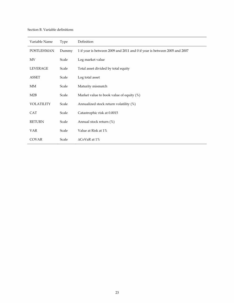
Section B. Variable definitions

Variable Name Type Definition

POSTLEHMAN Dummy 1 if year is between 2009 and 2011 and 0 if year is between 2005 and 2007

MV Scale Log market value

LEVERAGE Scale Total asset divided by total equity

ASSET Scale Log total asset

MM Scale Maturity mismatch

M2B Scale Market value to book value of equity (%)

VOLATILITY Scale Annualized stock return volatility (%)

CAT Scale Catastrophic risk at 0.0015

RETURN Scale Annual stock return (%)

VAR Scale Value at Risk at 1%

COVAR Scale ∆CoVaR at 1%

24

Table II. Summary statistics

Variable Mean Standard Deviation Min Max

POSTLEHMAN 0.50 0.51 0 1

MV 13.44 1.91 7.90 19.18

LEVERAGE 7.88 5.34 1 31.73

ASSET 8.11 1.95 1.99 14.71

MM 0.06 0.09 0 0.90

M2B 1.67 1.65 0 21.27

VOLATILITY 0.41 0.21 0.11 1.544

CAT (%) -15.26 11.66 -138.62 -3.54

RETURN (%) 1.32 11.09 -1.79 269.08

VAR (%) -13.74 9.59 -93.33 -4.31

COVAR (%) -2.79 2.04 -11.51 3.68

25

Table III. Correlation matrix Section A. Sample with data prior and post the Lehman bankruptcy This sample excludes the observations in 2008 when Lehman Brothers filed for Chapter 11, and we take the average values for each variable for the period prior to the bankruptcy (2005-2007) and the period after the bankruptcy (2009-2011).

PO

STL

EH

MA

N

MV

LE

VE

RA

GE

ASS

ET

MM

M2B

VO

LA

TIL

ITY

CA

T

RE

TU

RN

VA

R

MV -0.09

LEVERAGE -0.01 -0.18

ASSET 0.07 0.76 0.37

MM -0.07 0.02 0.22 0.14

M2B -0.22 0.20 -0.20 -0.21 -0.08

VOLATILITY 0.65 -0.34 0.15 -0.08 -0.03 -0.23

CAT -0.42 0.18 -0.12 -0.03 -0.02 0.18 -0.75

RETURN -0.02 0.00 0.00 -0.01 0.14 -0.02 0.06 -0.03

VAR -0.14 0.10 -0.04 0.01 -0.08 0.08 -0.43 0.35 -0.67

COVAR -0.16 -0.41 0.10 -0.30 0.06 -0.16 0.06 -0.01 0.13 -0.20

26

Section B. Sample with data from 2005 to 2011 This sample includes the entire dataset from 2005 to 2011, excluding 2008 when Lehman Brothers filed for Chapter 11.

MV

LE

VE

RA

GE

ASS

ET

MM

M2B

VO

LA

TIL

ITY

CA

T

RE

TU

RN

VA

R

LEVERAGE -0.15

ASSET 0.75 0.38

MM 0.02 0.23 0.15

M2B 0.25 -0.18 -0.19 -0.08

VOLATILITY -0.27 0.12 -0.03 0.00 -0.25

CAT 0.20 -0.10 0.00 -0.01 0.22 -0.86

RETURN 0.00 0.03 0.00 0.14 -0.02 0.05 -0.02

VAR 0.11 -0.05 -0.01 -0.10 0.13 -0.49 0.43 -0.61

COVAR -0.36 0.08 -0.28 0.03 -0.14 -0.12 0.14 0.12 -0.07

Table IV. Regressions of catastrophic and systemic risk prior and post Lehman bankruptcy

The dependent variables are the catastrophic risk of individual institutions and their systemic risk. The independent variables include the post-Lehman dummy, log market value, leverage, log total asset, maturity mismatch, market to book, stock return volatility, annual stock return, and value at risk at 1%. All specifications use OLS regression, and t-statistics are shown in the parentheses with ***, ** and * indicating its statistical significant level of 1%, 5% and 10% respectively.

Catastrophic Risk Systemic Risk Dependent Variable:

(1) (2) (3) (4)

POSTLEHMAN 3.126*** (5.229)

2.801*** (4.719)

-0.881*** (-6.312)

-0.909*** (-6.486)

MV -0.119

(-0.305) -0.153

(-0.385) -0.223**

(-2.449) -0.254*** (-2.709)

LEVERAGE 0.117

(1.496) 0.109

(1.351) 0.0357*

(1.948) 0.0351* (1.837)

ASSET -0.579

(-1.481) -0.483

(-1.212) -0.210**

(-2.295) -0.170* (-1.803)

MM -4.793** (-2.109)

-6.309*** (-2.627)

0.501 (0.944)

0.200 (0.352)

M2B 0.0766 (0.406)

-0.0639 (-0.337)

-0.222*** (-5.038)

-0.229*** (-5.123)

VOLATILITY -47.96*** (-26.91)

-47.44*** (-26.43)

-0.310 (-0.744)

-0.331 (-0.782)

RETURN 0.0866***

(3.119) 0.0918***

(3.344) -0.00599

(-0.924) -0.00548 (-0.845)

VAR 0.0875** (2.431)

0.0848** (2.380)

-0.0479*** (-5.701)

-0.0485*** (-5.764)

CONSTANT 9.380*** (3.164)

9.358*** (3.144)

1.882*** (2.718)

1.982*** (2.821)

Industry Fixed-effects No Yes

No Yes

N 1,281 1,281 1,281 1,281

R-square 0.58 0.60 0.26 0.27

F-test 196.89 132.29 49.13 32.36

28

Table V. Regressions of catastrophic and systemic risk with industry clustered standard error

The dependent variables are the catastrophic risk of individual institutions and their systemic risk. The independent variables include a post-Lehman dummy, log market value, leverage, log total asset, maturity mismatch, market to book, stock return volatility, annual stock return, and value at risk at 1%. All specifications use OLS regression, and t-statistics using industry clustered standard error on are shown in the parentheses with ***, ** and * indicating its statistical significant level of 1%, 5% and 10% respectively.

Catastrophic Risk Systemic Risk Dependent Variable:

(1) (2) (3) (4)

POSTLEHMAN 3.126** (3.024)

2.801** (2.677)

-0.881*** (-4.745)

-0.909*** (-5.143)

MV -0.119

(-0.130) -0.153

(-0.177) -0.223

(-1.585) -0.254

(-1.460)

LEVERAGE 0.117

(0.583) 0.109

(0.451) 0.0357

(1.624) 0.0351 (1.191)

ASSET -0.579

(-0.548) -0.483

(-0.425) -0.210

(-1.468) -0.170

(-0.927)

MM -4.793

(-1.726) -6.309

(-1.722) 0.501

(0.660) 0.200

(0.275)

M2B 0.0766 (0.236)

-0.0639 (-0.235)

-0.222** (-3.272)

-0.229** (-2.789)

VOLATILITY -47.96*** (-10.64)

-47.44*** (-9.633)

-0.310 (-0.449)

-0.331 (-0.460)

RETURN 0.0866***

(4.089) 0.0918***

(4.737) -0.00599

(-1.108) -0.00548 (-1.059)

VAR 0.0875 (1.542)

0.0848 (1.465)

-0.0479*** (-4.992)

-0.0485*** (-4.875)

CONSTANT 9.380

(1.751) 9.358

(1.853) 1.882*

(2.076) 1.982

(1.890)

Industry Fixed-effects No Yes

No Yes

N 1,281 1,281 1,281 1,281

R-square 0.59 0.60 0.26 0.27

29

Table VI. Regressions of catastrophic and systemic risk prior and post Lehman bankruptcy using annual data The dependent variables are the catastrophic risk of individual institutions and their systemic risk. The independent variables include a post-Lehman dummy, log market value, leverage, log total asset, maturity mismatch, market to book, stock return volatility, annual stock return, and value at risk at 1%. All specifications use OLS regression, and t-statistics are shown in the parentheses with ***, ** and * indicating its statistical significant level of 1%, 5% and 10% respectively.

Catastrophic Risk Systemic Risk Dependent Variable:

(1) (2) (3) (4) (5) (6) (7) (8)

MV -0.308** (-2.373)

-0.349*** (-2.618)

-0.308** (-2.373)

-0.349*** (-2.618)

-0.239*** (-4.608)

-0.266*** (-4.978)

-0.239*** (-4.608)

-0.266*** (-4.978)

LEVERAGE 0.00768 (0.297)

0.00751 (0.281)

0.00768 (0.297)

0.00751 (0.281)

0.0333***

(3.231) 0.0326***

(3.052) 0.0333***

(3.231) 0.0326***

(3.052)

ASSET 0.110

(0.840) 0.177

(1.313) 0.110

(0.840) 0.177

(1.313)

-0.191*** (-3.642)

-0.154*** (-2.857)

-0.191*** (-3.642)

-0.154*** (-2.857)

MM -1.650** (-2.215)

-2.434*** (-3.087)

-1.650** (-2.215)

-2.434*** (-3.087)

0.375

(1.262) 0.0956 (0.303)

0.375 (1.262)

0.0956 (0.303)

M2B 0.158** (2.267)

0.104 (1.470)

0.158** (2.267)

0.104 (1.470)

-0.230*** (-8.293)

-0.239*** (-8.491)

-0.230*** (-8.293)

-0.239*** (-8.491)

VOLATILITY -31.52*** (-64.58)

-31.47*** (-63.91)

-31.52*** (-64.58)

-31.47*** (-63.91)

-0.493** (-2.531)

-0.516*** (-2.620)

-0.493** (-2.531)

-0.516*** (-2.620)

RETURN 0.0435***

(5.070) 0.0459***

(5.378) 0.0435***

(5.070) 0.0459***

(5.378)

0.000859 (0.251)

0.00135 (0.394)

0.000859 (0.251)

0.00135 (0.394)

VAR 0.0356***

(3.108) 0.0348***

(3.041) 0.0356***

(3.108) 0.0348***

(3.041)

-0.0377*** (-8.243)

-0.0383*** (-8.351)

-0.0377*** (-8.243)

-0.0383*** (-8.351)

2005 DUMMY -0.994*** (-3.589)

-0.879*** (-3.176)

0.678*** (6.131)

0.710*** (6.418)

2006 DUMMY -0.863*** (-3.109)

-0.745*** (-2.686)

0.131 (0.511)

0.134 (0.525)

0.804*** (7.250)

0.836*** (7.538)

0.126 (1.226)

0.126 (1.230)

2007 DUMMY -0.717*** (-2.697)

-0.639** (-2.410)

0.277 (1.068)

0.240 (0.928)

0.176* (1.656)

0.197* (1.861)

-0.503*** (-4.846)

-0.513*** (-4.958)

2009 DUMMY 2.533*** (8.753)

2.518*** (8.705)

3.527*** (10.44)

3.396*** (10.07)

-1.002*** (-8.671)

-0.996*** (-8.611)

-1.680*** (-12.46)

-1.707*** (-12.65)

2010 DUMMY 0.453* (1.758)

0.472* (1.841)

1.447*** (5.335)

1.351*** (4.993)

0.187* (1.824)

0.193* (1.884)

-0.491*** (-4.533)

-0.517*** (-4.780)

2011 DUMMY 0.994*** (3.589)

0.879*** (3.176)

-0.678*** (-6.131)

-0.710*** (-6.418)

CONSTANT 5.926*** (6.147)

5.920*** (6.085)

4.931*** (5.053)

5.041*** (5.114)

1.615*** (4.196)

1.659*** (4.262)

2.293*** (5.886)

2.370*** (6.008)

Industry Fixed-effects No Yes No Yes No Yes No Yes

N 3,851 3,851 3,851 3,851 3,851 3,851 3,851 3,851

R-square 0.71 0.71 0.71 0.72 0.26 0.27 0.26 0.27

F-test 723.35 529.51 723.55 529.51 102.47 75.77 102.47 75.77

30

Table VII. Regressions of catastrophic and systemic risk using annual data with industry clustered standard error The dependent variables are the catastrophic risk of individual institutions and their systemic risk. The independent variables include a post-Lehman dummy, log market value, leverage, log total asset, maturity mismatch, market to book, stock return volatility, annual stock return, and value at risk at 1%. All specifications use OLS regression, and t-statistics using industry clustered standard error on are shown in the parentheses with ***, ** and * indicating its statistical significant level of 1%, 5% and 10% respectively.

Catastrophic Risk Systemic Risk Dependent Variable:

(1) (2) (3) (4) (5) (6) (7) (8)

MV -0.308

(-0.819) -0.349

(-0.990) -0.308

(-0.819) -0.349

(-0.990)

-0.239 (-1.775)

-0.266 (-1.642)

-0.239 (-1.775)

-0.266 (-1.642)

LEVERAGE 0.00768 (0.127)

0.00751 (0.106)

0.00768 (0.127)

0.00751 (0.106)

0.0333 (1.519)

0.0326 (1.185)

0.0333 (1.519)

0.0326 (1.185)

ASSET 0.110

(0.304) 0.177

(0.468) 0.110

(0.304) 0.177

(0.468)

-0.191 (-1.340)

-0.154 (-0.865)

-0.191 (-1.340)

-0.154 (-0.865)

MM -1.650** (-3.701)

-2.434* (-2.389)

-1.650** (-3.701)

-2.434* (-2.389)

0.375

(0.559) 0.0956 (0.150)

0.375 (0.559)

0.0956 (0.150)

M2B 0.158

(0.940) 0.104

(0.818) 0.158

(0.940) 0.104

(0.818)

-0.230** (-3.335)

-0.239** (-2.918)

-0.230** (-3.335)

-0.239** (-2.918)

VOLATILITY -31.52*** (-14.96)

-31.47*** (-14.24)

-31.52*** (-14.96)

-31.47*** (-14.24)

-0.493

(-0.880) -0.516

(-0.887) -0.493

(-0.880) -0.516

(-0.887)

RETURN 0.0435** (3.799)

0.0459** (4.028)

0.0435** (3.799)

0.0459** (4.028)

0.000859 (0.140)

0.00135 (0.222)

0.000859 (0.140)

0.00135 (0.222)

VAR 0.0356* (2.243)

0.0348* (2.350)

0.0356* (2.243)

0.0348* (2.350)

-0.0377** (-4.003)

-0.0383** (-3.889)

-0.0377** (-4.003)

-0.0383** (-3.889)

2005 DUMMY -0.994

(-1.538) -0.879

(-1.396)

0.678*** (4.968)

0.710*** (5.827)

2006 DUMMY -0.863

(-1.023) -0.745

(-0.902) 0.131

(0.611) 0.134

(0.631)

0.804*** (7.761)

0.836*** (9.478)

0.126** (2.664)

0.126** (2.632)

2007 DUMMY -0.717

(-1.041) -0.639

(-0.955) 0.277

(1.636) 0.240

(1.217)

0.176 (1.114)

0.197 (1.383)

-0.503*** (-6.038)

-0.513*** (-5.860)

2009 DUMMY 2.533*** (4.767)

2.518*** (4.714)

3.527*** (6.580)

3.396*** (6.376)

-1.002*** (-16.18)

-0.996*** (-14.59)

-1.680*** (-8.662)

-1.707*** (-9.149)

2010 DUMMY 0.453

(0.901) 0.472

(0.919) 1.447*** (4.558)

1.351*** (5.010)

0.187*** (9.435)

0.193*** (8.088)

-0.491** (-3.172)

-0.517** (-3.591)

2011 DUMMY 0.994*** (3.538)

0.879*** (3.396)

-0.678*** (-4.968)

-0.710*** (-5.827)

CONSTANT 5.926

(1.786) 5.920

(1.815) 4.931

(1.778) 5.041

(1.845)

1.615 (1.770)

1.659 (1.662)

2.293** (2.895)

2.370** (2.656)

Industry Fixed-effects No Yes No Yes No Yes No Yes

N 3,851 3,851 3,851 3,851 3,851 3,851 3,851 3,851

R-square 0.71 0.72 0.71 0.72 0.26 0.27 0.26 0.27

31

Table VIII. Difference-in-difference regressions of catastrophic risk and systemic risk Section A. Industries included in the control group

SIC Code Industry Name

0100 AGRICULTURAL PRODUCTION-CROPS 0200 AGRICULTURAL PROD-LIVESTOCK & ANIMAL SPECIALTIES 0700 AGRICULTURAL SERVICES 0800 FORESTRY 0900 FISHING, HUNTING AND TRAPPING 1000 METAL MINING 1040 GOLD AND SILVER ORES 1090 MISCELLANEOUS METAL ORES 1220 BITUMINOUS COAL & LIGNITE MINING 1221 BITUMINOUS COAL & LIGNITE SURFACE MINING 1311 CRUDE PETROLEUM & NATURAL GAS 1381 DRILLING OIL & GAS WELLS 1382 OIL & GAS FIELD EXPLORATION SERVICES 1389 OIL & GAS FIELD SERVICES, NEC 1400 MINING & QUARRYING OF NONMETALLIC MINERALS (NO FUELS) 1520 GENERAL BLDG CONTRACTORS - RESIDENTIAL BLDGS 1531 OPERATIVE BUILDERS 1540 GENERAL BLDG CONTRACTORS - NONRESIDENTIAL BLDGS 1600 HEAVY CONSTRUCTION OTHER THAN BLDG CONST - CONTRACTORS 1623 WATER, SEWER, PIPELINE, COMM & POWER LINE CONSTRUCTION 1700 CONSTRUCTION - SPECIAL TRADE CONTRACTORS 1731 ELECTRICAL WORK 2000 FOOD AND KINDRED PRODUCTS 2011 MEAT PACKING PLANTS 2013 SAUSAGES & OTHER PREPARED MEAT PRODUCTS 2015 POULTRY SLAUGHTERING AND PROCESSING 2020 DAIRY PRODUCTS 2024 ICE CREAM & FROZEN DESSERTS 2030 CANNED, FROZEN & PRESERVD FRUIT, VEG & FOOD SPECIALTIES 2033 CANNED, FRUITS, VEG, PRESERVES, JAMS & JELLIES 2040 GRAIN MILL PRODUCTS 2050 BAKERY PRODUCTS 2052 COOKIES & CRACKERS 2060 SUGAR & CONFECTIONERY PRODUCTS 2070 FATS & OILS 2080 BEVERAGES 2082 MALT BEVERAGES 2086 BOTTLED & CANNED SOFT DRINKS & CARBONATED WATERS 2090 MISCELLANEOUS FOOD PREPARATIONS & KINDRED PRODUCTS 2092 PREPARED FRESH OR FROZEN FISH & SEAFOODS 2100 TOBACCO PRODUCTS 2111 CIGARETTES 2200 TEXTILE MILL PRODUCTS 2211 BROADWOVEN FABRIC MILLS, COTTON 2221 BROADWOVEN FABRIC MILLS, MAN MADE FIBER & SILK 2250 KNITTING MILLS 2253 KNIT OUTERWEAR MILLS 2273 CARPETS & RUGS 2300 APPAREL & OTHER FINISHD PRODS OF FABRICS & SIMILAR MATL

32

2320 MEN'S & BOYS' FURNISHGS, WORK CLOTHG, & ALLIED GARMENTS 2330 WOMEN'S, MISSES', AND JUNIORS OUTERWEAR 2340 WOMEN'S, MISSES', CHILDREN'S & INFANTS' UNDERGARMENTS 2390 MISCELLANEOUS FABRICATED TEXTILE PRODUCTS 2400 LUMBER & WOOD PRODUCTS (NO FURNITURE) 2421 SAWMILLS & PLANTING MILLS, GENERAL 2430 MILLWOOD, VENEER, PLYWOOD, & STRUCTURAL WOOD MEMBERS 2451 MOBILE HOMES 2452 PREFABRICATED WOOD BLDGS & COMPONENTS 2510 HOUSEHOLD FURNITURE 2511 WOOD HOUSEHOLD FURNITURE, (NO UPHOLSTERED) 2520 OFFICE FURNITURE 2522 OFFICE FURNITURE (NO WOOD) 2531 PUBLIC BLDG & RELATED FURNITURE 2540 PARTITIONS, SHELVG, LOCKERS, & OFFICE & STORE FIXTURES 2590 MISCELLANEOUS FURNITURE & FIXTURES 2600 PAPERS & ALLIED PRODUCTS 2611 PULP MILLS 2621 PAPER MILLS 2631 PAPERBOARD MILLS 2650 PAPERBOARD CONTAINERS & BOXES 2670 CONVERTED PAPER & PAPERBOARD PRODS (NO CONTANERS/BOXES) 2673 PLASTICS, FOIL & COATED PAPER BAGS 2711 NEWSPAPERS: PUBLISHING OR PUBLISHING & PRINTING 2721 PERIODICALS: PUBLISHING OR PUBLISHING & PRINTING 2731 BOOKS: PUBLISHING OR PUBLISHING & PRINTING 2732 BOOK PRINTING 2741 MISCELLANEOUS PUBLISHING 2750 COMMERCIAL PRINTING 2761 MANIFOLD BUSINESS FORMS 2771 GREETING CARDS 2780 BLANKBOOKS, LOOSELEAF BINDERS & BOOKBINDG & RELATD WORK 2790 SERVICE INDUSTRIES FOR THE PRINTING TRADE 2800 CHEMICALS & ALLIED PRODUCTS 2810 INDUSTRIAL INORGANIC CHEMICALS 2820 PLASTIC MATERIAL, SYNTH RESIN/RUBBER, CELLULOS (NO GLASS) 2821 PLASTIC MATERIALS, SYNTH RESINS & NONVULCAN ELASTOMERS 2833 MEDICINAL CHEMICALS & BOTANICAL PRODUCTS 2834 PHARMACEUTICAL PREPARATIONS 2835 IN VITRO & IN VIVO DIAGNOSTIC SUBSTANCES 2836 BIOLOGICAL PRODUCTS, (NO DISGNOSTIC SUBSTANCES) 2840 SOAP, DETERGENTS, CLEANG PREPARATIONS, PERFUMES, COSMETICS 2842 SPECIALTY CLEANING, POLISHING AND SANITATION PREPARATIONS 2844 PERFUMES, COSMETICS & OTHER TOILET PREPARATIONS 2851 PAINTS, VARNISHES, LACQUERS, ENAMELS & ALLIED PRODS 2860 INDUSTRIAL ORGANIC CHEMICALS 2870 AGRICULTURAL CHEMICALS 2890 MISCELLANEOUS CHEMICAL PRODUCTS 2891 ADHESIVES & SEALANTS 2911 PETROLEUM REFINING 2950 ASPHALT PAVING & ROOFING MATERIALS 2990 MISCELLANEOUS PRODUCTS OF PETROLEUM & COAL

33

Section B. Difference-in-difference regression analysis We consider the Bear Stearns and Lehman Brothers bankruptcies in 2008 as an exogenous shock, and employ a difference-in-differences (DiD) approach (see Meyer 1995, and Angrist and Krueger 1999 for detailed explanations of this methodology) to study the causal effects. All financial institutions are defined as the treatment group, and firms with SIC code 00-30 are defined as the non-treated group. The dummy variable TREATMENT is set to one for financial institutions after 2008 and zero otherwise. The dummy variable POSTLEHMAN is set to one if it is after 2008, and zero otherwise. A third dummy variable POSTLEHMAN×TREATMENT is the cross-product of the previous two dummy variables. The dependent variables are catastrophic risk of individual institutions and their systemic risk. The independent variables include log market value, leverage, log total asset, maturity mismatch, market to book, stock return volatility, annual stock return, and value at risk at 1%. The specifications (2), (3), (5) and (6) use firm fixed-effects and the specifications (3) and (6) use clustered standard error on industry. z-statistics are shown in the parentheses with ***, ** and * indicating its statistical significant level of 1%, 5% and 10% respectively.

Catastrophic Risk Systemic Risk Dependent Variable:

(1) (2) (3) (4) (5) (6)

POSTLEHMAN 3.560*** (5.517)

3.800*** (6.032)

3.800*** (6.991)

-0.385*** (-3.323)

-0.416*** (-3.649)

-0.416*** (-3.870)

TREATMENT -1.563** (-2.261)

-4.371 (-0.812)

-4.371*** (-5.122)

0.272** (2.195)

1.023 (1.049)

1.023*** (15.23)

POSTLEHMAN×TREATMENT 0.756** (1.898)

0.905** (2.104)

0.905** (1.935)

-0.455*** (-3.012)

-0.486*** (-3.272)

-0.486*** (-3.766)

MV -0.340

(-1.048) -0.501

(-1.537) -0.501

(-0.810)

-0.261*** (-4.493)

-0.262*** (-4.429)

-0.262*** (-4.597)

LEVERAGE 0.108

(1.380) 0.154* (1.865)

0.154 (1.101)

0.0240* (1.703)

0.0174 (1.160)

0.0174 (0.812)

ASSET -0.110

(-0.349) -0.120

(-0.379) -0.120

(-0.195)

-0.152*** (-2.685)

-0.119** (-2.078)

-0.119** (-2.204)

MM -5.327* (-1.925)

-6.320** (-2.232)

-6.320*** (-2.966)

0.667

(1.344) 0.428

(0.834) 0.428

(0.678)

M2B -0.182* (-1.713)

-0.130 (-1.246)

-0.130 (-1.046)

-0.0811***

(-4.250) -0.0830***

(-4.391) -0.0830** (-2.107)

VOLATILITY -54.34*** (-33.96)

-56.00*** (-34.87)

-56.00*** (-10.88)

0.0379 (0.132)

0.206 (0.708)

0.206 (0.490)

RETURN 0.0290** (2.305)

0.0335*** (2.708)

0.0335 (1.091)

0.00326 (1.446)

0.00195 (0.872)

0.00195 (0.880)

VAR 0.0674** (2.309)

0.0625** (2.179)

0.0625 (0.773)

-0.0312***

(-5.951) -0.0326***

(-6.277) -0.0326***

(-3.668)

CONSTANT 12.46*** (4.403)

17.18*** (3.082)

17.18** (2.562)

1.558*** (3.069)

1.177 (1.165)

1.177** (2.086)

Industry Fixed-effects No Yes Yes No Yes Yes

Clustered Standard Error No No Yes No No Yes

N 2,376 2,376 2,376 2,376 2,376 2,376

R-square 0.52 0.55 0.55 0.24 0.27 0.27