Has India Emerged ? Business Cycle StylizedFacts from a Transitioning Economy

Chetan Ghate∗ Radhika Pandey† Ila Patnaik‡§

April 11, 2011

Abstract

This paper presents a comprehensive set of stylised facts for busi-ness cycles in India from 1950 - 2009. We find that the nature of thebusiness cycle has changed dramatically after India’s liberalisation re-forms in 1991. In particular, after the the mid 1990s, the propertiesof India’s business cycle has moved closer in key respects to selectadvanced countries. This is consistent with India’s structural trans-formation from a pre-dominantly agricultural and planned developingeconomy to a more market based industrial-income economy. We alsoidentify in what respects the behaviour of the Indian business cycle isdifferent from that of other advanced economies, and closer to that ofother less developed economies. This is the first exercise of this kindto generate an exhaustive set of stylised facts for India using bothannual and quarterly data.

JEL Classification: E10, E32Keywords: Macroeconomics, Real Business Cycles, Emerging Market DSGEModels, Volatility and Growth.

∗Indian Statistical Institute- Delhi Center, New Delhi-110016, India†National Institute of Public Finance and Policy, New Delhi-110067, India‡National Institute of Public Finance and Policy, New Delhi-110067, India§This paper was written under the aegis of the SPF Financial and Monetary Policy

Reform Project at the National Institute for Public Finance and Policy, New Delhi. Weare grateful to Abhijit Banerjee for comments. We also thank participants at the ‘Busi-ness Cycle Facts and DSGE Model for India’ workshop at NIPFP, the Eighth meetingof the NIPFP-DEA Research Program, and Workshop 5 of the Center for InternationalMacroeconomic Studies (Surrey University) for useful comments.

1

Contents

1 Introduction 3

2 Stylised Facts from Emerging Economies 6

3 India in Transition 9

4 The Dataset 12

5 Statistical Methodology 13

6 Indian Business Cycle Stylised Facts in the Pre and PostReform Period 15

7 Robustness Checks 187.1 Stylised Facts with Quarterly Data . . . . . . . . . . . . . . . 187.2 An Alternative Detrending Method . . . . . . . . . . . . . . . 227.3 Redefining the Sample Period . . . . . . . . . . . . . . . . . . 23

8 Conclusion 24

A Data Definition and Sources 29

2

1 Introduction

This paper describes the changing nature of the Indian business cycle from1950 - 2009. Our focus is to compare India’s business cycle in the pre 1991economy, with the post 1991 Indian economy, after the large scale liberal-ization reforms of 1991. Our main finding is that after the liberalisation ofthe Indian economy in 1991, the properties of the Indian business cycle lookcloser to that of advanced industrialized economies in several key respects.This paper - to the best of our knowledge - is the first such exercise to com-prehensively document changes in the properties of the Indian business cyclein the pre and post reform period.

A large literature documents business cycle stylised facts both in advancedindustrial economies (Kydland and Prescott, 1990; Backus and Kehoe, 1992;Stock and Watson, 1999; King and Rebelo, 1999) as well as developing andemerging market economies (Agenor et al., 2000; Rand and Tarp, 2002; Male,2010). Agenor et al. (2000) present a comparison of the business cycle prop-erties of developed and developing economies based on a quarterly datasetfrom first quarter of 1978 to the fourth quarter of 1995. The Index of in-dustrial production (IIP) is taken as a proxy for aggregate business activ-ity. Cyclical components of variables are derived using both the Hodrick-Prescott and Baxter-King filters. A main finding of the paper is that devel-oping economies are characterized by higher output volatility compared todeveloped economies. Similarly, Rand and Tarp (2002) report business cyclestylised facts for 15 developing economies based on an annual dataset from1970-1997. gdp is taken as a proxy for aggregate business activity. Theseauthors find that output volatility in developing economies is 15-20% higherthan that of developed countries. They also find that consumption is morevolatile than output for developing economies (with South Africa and Indiaas exceptions). Volatility in investment is found to be similar to developedeconomies. However, they do not find any consistent evidence of counter-cyclical government expenditure in their sample of developing economies.1

Other papers in the literature - such as Neumeyer and Perri (2005) - alsoprovide a comparison of business cycle properties of a set of five emergingeconomies with a set of five developed economies. gdp is taken as a proxy for

1Rand and Tarp (2002) find a positive relation between consumption and output exceptfor Nigeria. Higher volatility in investment is found to be pro-cyclical in all the developingcountries included in the sample. While imports are reported to be pro-cyclical, the pictureregarding exports is unclear. On the relation between price level and output, the picture isunclear with seven of the developing economies reporting significant negative correlationbetween price level and output.

3

aggregate business cycle activity. Output volatility is found to be higher foremerging economies. While the relative volatility of consumption is greaterthan 1 for emerging economies, the relative volatility of investment is uniformacross the two set of countries. Similarly, Alper (2002) analyses business cy-cles in Mexico and Turkey from 1987-2000 and presents a comparison of theresults with the United States. Consistent with the business cycle featuresof developing economies, the volatility of real gdp in Mexico and Turkey arefound to be 2.63 and 3.91 times larger than for the United States. Consump-tion is found to be more volatile than output in these economies.

Finally, Male (2010) provides a comprehensive documentation of cross-countrycomparison of business cycle stylised facts. Her paper relies on a quarterlydataset for 32 developing economies, across different regions, of which Indiais part of the sample for Asian countries. Due to lack of reliable data onreal gdp for a number of developing economies, she uses indexes of indus-trial production as a proxy for the aggregate business cycle. Business cycleproperties of developing economies are found to be distinctly different fromthose of developed economies. Key variables like output, private consump-tion, price levels are more volatile in developing economies. The correlationof investment and imports with the aggregate business cycle is not found tobe very strong. Government expenditure is not significantly counter-cyclical,unlike in developed countries. Business cycle characteristics also differ interms of persistence of variables. For instance, the persistence of outputand price levels are lower for developing economies compared with developedeconomies.

Because India is typically treated as one of many countries within a largersample (see (Agenor et al., 2000; Rand and Tarp, 2002; Male, 2010)), suchstudies do not show the changing nature of the business cycle of any particularcountry over time. Our main contribution is to provide evidence on thechanging stylised facts of the Indian economy from 1950 - 2009. During thistime, India transitioned from a closed and protected economy characterisedby controls on capacity creation and high import duties, to an economy wellintegrated with the world, with the policy environment changing significantlyin 1991. In terms of business cycle fluctuations, the economy moved awayfrom monsoon cycles (Patnaik and Sharma, 2002) to business cycles in theconventional sense.

The empirical literature on stylised facts relies on long time series of quarterlydata. However, quarterly gdp data in India is available only from 1999. Thislimits us to 11 years of quarterly data for our key variables. Hence, sincewe are interested in the changing pattern of the Indian business cycle, we

4

conduct our analysis with annual data and then use the quarterly data tocheck the robustness of our results.

In particular, we are interested in the properties of Indian business cycleover two periods: 1950-1991 for the pre-liberalisation period and 1992-2009for the post-liberalisation period. gdp, private consumption, total gross fixedcapital formation, consumer prices, exports, imports, government expendi-ture and nominal exchange rate are the key variables analysed. Since thequantitative general equilibrium literature also seeks to explain the strongcounter-cyclicality of net exports as well as highly volatile and counter cycli-cal interest rates in emerging markets, we also report the business cycleproperties of these variables for India. Our main finding is to highlight thedifference in the properties of the Indian business cycle stylised over the twoperiods, and suggest reasons for these changes. A data appendix lists all thesources and definitions of variables used in this study.

In terms of similarities, we find that output (Real gdp) has become lessvolatile in the post-liberalisation period; investment has become significantlypro-cyclical in the post-liberalisation period; the correlation of imports withgdp has also increased; net exports have become counter-cyclical; the volatil-ity in prices and government expenditure has decreased in the post liberalisa-tion period; and the absolute volatility in nominal exchange rate has declined.Further, our results using quarterly data are consistent with the findings ofthe annual data analysis for the post 1991 period. This suggests that inmany key respects, the Indian business cycle shows a growing resemblancewith those of the developed economies.

In terms of differences, the Indian business cycle features also resemble fea-tures of developing economies. While output volatility has fallen, it stillremains high. In addition, consumption is more volatile than output. Fur-ther, government expenditure is not strongly counter-cyclical with respect tooutput, as in advanced economies.

In terms of the sensitivity tests, we note that the volatility of consumption issensitive to the choice of the de-trending procedure. The absolute volatility ofprivate consumption falls in the post-reform period when the band pass filterof Baxter-King is used to de-trend the series. However, the absolute volatilityis higher in the post-reform period when the Hodrick-Prescott filter is usedto de-trend the series. There is also a significant reduction in volatility ofgovernment expenditure when the Baxter-King filter is used to de-trend theseries. However, the key feature of the Indian business cycle which is robustto de-trending procedures is the significant pro-cyclicality of investment withoutput. Coupled with the increased pro-cyclicality of imports with output,

5

this feature makes the Indian business cycle stylised facts closer to those ofthe advanced economies.

The remainder of the paper is divided into the following sections. Section2 outlines the main features of emerging economies business cycle with anoverview of the sources of shocks in these economies. Section 3 presents asnapshot of India’s transition. Section 4 outlines the data sources and thevariables included in the study. Section 5 details the methodology employedto compute the Indian business cycle stylised facts. Section 6 provides em-pirical evidence on the changing Indian business cycle stylised facts from preto post reform period. Section 7 presents results on sensitivity tests. Section8 concludes.

2 Stylised Facts from Emerging Economies

As noted in the introduction, one of the main features that distinguishesemerging economies business cycles from advanced economies is their highervolatility. Current account balances, output growth, interest rates, and ex-change rate tend to exhibit larger, and more frequent changes (Calderon andFuentes, 2006). There are other aspects that characterize emerging mar-ket economies: consumption is more volatile than output with a relativevolatility larger than one; real interest rates are highly volatile and countercyclical, and net exports are strongly counter-cyclical (Neumeyer and Perri,2005; Aguiar and Gopinath, 2007; Uribe and Yue, 2006).2

As a point of reference, we reproduce Table 1 from Aguiar and Gopinath(2007).3 The analysis covers 13 developed and 13 emerging economies basedon a quarterly dataset.4 The findings in Table 1 are broadly consistent with

2Empirical work on emerging market business cycles has led to quantitative generalequilibrium models both in the RBC and DSGE tradition on understanding the keyproperties of emerging market business cycle fluctuations (Aguiar and Gopinath, 2007;Chakraborty, 2008; Neumeyer and Perri, 2005; Uribe and Yue, 2006; Batini et al., 2010;Gabriel et al., 2010; Garcia-Cicco et al., 2010).

3We refer to this paper as it provides average figures for business cycle characteristicsfor developed and developing economies. This facilitates locating the position of Indianbusiness cycle vis-a-vis developed and developing economies.

4Australia, Austria, Belgium, Canada, Denmark, Finland, Netherlands, New Zealand,Norway, Portugal, Spain, Sweden and Switzerland comprise the sample of developedeconomies while Argentina, Brazil, Ecuador, Israel, Korea, Malaysia, Mexico, Peru, Philip-pines, Slovak Republic, South Africa, Thailand and Turkey comprise the set of emergingeconomies.

6

the findings of other papers on the business cycle stylised facts of developingeconomies.

Table 1 Business cycle statistics for developed and emerging economies usingquarterly data

Developed economies Emerging economies

Std Rel Cont. Std Rel. Cont.dev. std. dev. cor. dev. std. dev. cor.

Real gdp 1.34 1.00 1.00 2.74 1.00 1.00Private Consumption 0.94 0.66 1.45 0.72Investment 3.41 0.67 3.91 0.77Trade balance 1.02 -0.17 3.22 -0.51Source: Aguiar and Gopinath, 2007.

Table 1 shows that the business cycle characteristics of developed and emerg-ing economies differ on some important dimensions. Emerging economies,on an average have higher output volatility compared with the developedeconomies. Table 1 shows an average volatility of 1.34 for developed economiesand 2.74 for emerging economies. Another important difference is that con-sumption tends to be more volatile than output in emerging economies. Theaverage relative volatility of consumption is 1.45 for emerging economies and0.94 for developed economies. Relative investment volatility is compara-tively higher for emerging economies at 3.91, compared to 3.41 for developedeconomies.

A distinguishing feature of emerging economies business cycle is the strongcounter-cyclicality of trade balance at the business cycle frequencies. Accord-ing to Aguiar and Gopinath (2007), this property follows from the nature ofshocks governing fluctuations in developed and emerging economies. Theproductivity processes can be in the form of a transitory shock around thetrend growth rate of productivity and a stochastic trend growth rate. Inan emerging market setting, a shock to the growth rate implies a boost tocurrent output, but an even larger boost to future output. This implies thatconsumption responds more than income, reducing savings and generating acurrent account deficit. If growth shocks dominate transitory income shocks,the economy resembles a typical emerging market with its volatile consump-tion process and counter-cyclical current account. Conversely, a developedeconomy characterised by relatively stable growth process will be dominatedby standard, transitory productivity shocks. Such a shock will generate anincentive to save that will offset any increase in investment, resulting in lim-ited cyclicality of the current account. However, counter-cyclical net exports

7

is also reported for developed economies by Stock and Watson (1999); Randand Tarp (2002).

Aguiar and Gopinath (2007) use a standard RBC model to explain thebusiness cycle properties of emerging markets. Because emerging marketeconomies are characterized by frequent changes in economic policy, theyassume that shocks to trend growth are the primary source of fluctuations.This implies that the random walk component of the Solow residual is rela-tively larger. However, Calderon and Fuentes (2006) suggest that because thesources of shocks in Aguiar and Gopinath (2007) remain a black box, it is notclear whether these are being driven by changes in economic reforms, or othermarket frictions. Indeed, Chari et al. (2007) show that a variety of frictionscan be represented in reduced form as Solow residuals. Garcia-Cicco et al.(2010) show that when estimated over a long sample, the RBC model drivenby permanent and transitory shocks - a la Aguiar and Gopinath (2007) - doesa poor job in explaining observed business cycles in Argentina and Mexico,along a number of dimensions. These findings of Garcia-Cicco et al. (2010)suggest that the RBC model driven by productivity shocks does not providean adequate explanation of business cycles in emerging economies.

Other papers in the literature, such as Neumeyer and Perri (2005) emphasizethe interaction between foreign interest rate shocks and domestic financialfrictions that drive business cycle fluctuations in emerging market economies.Firms in their model demand working capital to finance their wage bill mak-ing labour demand sensitive to interest rate fluctuations. An increase in theemerging market country’s interest rate leads to a rise in labour costs. Sincelabour supply is insensitive to interest rate shocks, a lower demand for labourleads to lower levels of employment and output in equilibrium. Uribe andYue (2006) find that both country interest rates drive output fluctuationsin emerging market economies as well as the other way around. Kose et al.(2003) analyse the importance of domestic and external factors as causingcycles. Calvo (1998) argues that the idea of sudden stops are an importantfactor of large cycles in emerging markets.

A discussion of the sources of aggregate business cycle fluctuations assumesgreater relevance for a country like India that has undergone significant trans-formation since the early nineties. With high growth, there has been a sharpincrease in India’s integration on both trade and financial flows, possibly lead-ing to one source of volatility.5 Ramey and Ramey (1995) however find, that

5Jayaram et al. (2009) show that the integration with the global economy has alsoresulted in greater business cycle synchronisation with advanced economies and with theUS.

8

there is a negative correlation between volatility and growth. This wouldsuggest that whether India’s output is more volatile (compared to OECDeconomies), because it is growing faster, would seem unlikely, unless growthhas increased volatility and volatility itself reduces growth subsequently. Wetherefore think a plausible story of the changing pattern of the Indian busi-ness cycle is to link it with the policy regime. In particular, prior to 1991,positive productivity shocks could not be accommodated and generated in-flationary pressures and a worsening of the exchange rate. After the 1991reforms, the same shocks were permitted to generate growth, making invest-ment and imports go up, with foreign investment flowing in and the exchangerate appreciating. As in Aguiar and Gopinath (2007), consumption volatilityremained high mostly because of permanent productivity shocks, i.e., con-sumption volatility was driven by shocks to income that are larger or morepersistent than they should be. However, the focus of this paper is in docu-menting the changing nature of the Indian business cycle in the pre and postreform period.6

3 India in Transition

As mentioned earlier, a careful analysis of business cycle stylised facts assumegreater relevance for an economy like India that is subject to significanttransformation over the last two decades. In this section, we present some ofthe key elements of transformation in the Indian economy from 1950 - 2009.

1. Reduction in the consumption-output ratio: The first two plots of Fig-ure 1 show the behaviour of the consumption-output ratio and invest-ment output ratio from 1950-2009. The graphs show that while theshare of private consumption has declined, there is a gradual and con-sistent increase in the share of investment in gdp.

6Another source of volatility would be that productivity shocks get amplified by fric-tions as in (Aghion et al., 2004). Here, excess output volatility results because of capacityunder-utilization. Aghion et al. (2010) show however that there is not much evidence thatinvestment responds more to productivity shocks in economies with less good capital mar-kets. On the other hand, these authors also find that the fraction of long term investmentin total investment is more pro-cyclical in economies with less good capital markets. Iflong run investment enhances productivity, then the reform story implicit in this paperacquires salience.

9

Figure 1 The story of India’s transition

Sha

re o

f priv

ate

cons

umpt

ion

(Per

cen

t to

GD

P)

1950 1960 1970 1980 1990 2000 2010

6575

8595

Sha

re o

f inv

estm

ent (

Per

cen

t to

GD

P)

1950 1960 1970 1980 1990 2000 2010

1520

2530

35

Sha

re o

f agr

icul

ture

(P

er c

ent t

o G

DP

)

1950 1960 1970 1980 1990 2000 2010

2030

4050

Pub

lic s

ecto

r in

vest

men

t (P

er c

ent t

o to

tal)

1950 1960 1970 1980 1990 2000 2010

2535

4555

Priv

ate

corp

orat

e G

CF

(P

er c

ent t

o G

DP

)

1950 1960 1970 1980 1990 2000 2010

05

1015

Gro

ss fl

ows

(Per

cen

t to

GD

P)

1950 1960 1970 1980 1990 2000 2010

020

4060

capital accountcurrent account

In addition, since the mid 1990s, the Indian economy has undergonea significant transformation in many aspects. From a purely monsoondriven economy, fluctuations in the economy are now driven primarilyby fluctuations in inventory and investment. The share of investmentin gdp has increased from 13% in 1950-51 to 35% in 2009-10. Theincrease has been particularly prominent since 2004-05.

2. Declining share of agriculture: In the India of old, monsoon perfor-mance used to define a good or bad time. Adverse agricultural perfor-mance used to throw gdp growth off trend (Shah, 2008; Patnaik and

10

Sharma, 2002). In the India of present times, monsoon shocks mat-ter less. This is evident in the declining share of agriculture in Indiangdp. The third graph in Figure 1 shows a consistently declining shareof agriculture since 1950s. Table 2 shows the changing composition ofIndian gdp, the decline in the share of agriculture has been matchedwith a rise in the share of services.

Table 2 Changing composition of gdp

Agriculture Industry Services

1951 53.15 16.5 30.21992 28.8 27.4 442009 14.6 28.4 57

3. Shift away from state domination: An important dimension of India’stransition is the shift away from state domination towards a marketeconomy. This is visible in the fourth graph of Figure 1. The graphshows that the share of public investment in total investment surgedin the 1960s and 1970s. Since then it has been consistently declining.

4. Emergence of a conventional business cycle: The policy set up in In-dia of old times was characterised by controls on capacity creation andbarriers to trade. In such a scenario, conventional business cycles char-acterised by an interplay of inventories and investment did not exist.One prominent source of investment was government investment in theform of plan expenditure, which did not show any cyclical fluctuations.In the present environment with eased controls on capacity creationand dismantling of trade barriers, private sector investment as a shareof gdp has shown a significant rise.

The fifth graph in Figure 1 shows the time series of private corporategross capital formation expressed as a percent to gdp. In recent yearswe can see the emergence of the behaviour found in the conventionalbusiness cycle. In the investment boom of the mid-1990s, private cor-porate gcf rose from 5% of gdp in 1990-91 to 11% of gdp in 1995-96.This then fell dramatically in the business cycle downturn to 5.39%in 2001-02, and has since recovered to 17.6% in 2007-08. The recentrecession has led to its fall to 13.5% in 2009-10.

5. Increased integration with the rest of the world: The India of old wassheltered from external competition through high import duties andother barriers to trade. The capital account was also subject to strict

11

regulations on inflows and outflows. Since the adoption of liberalisationpolicy, the restrictions on current and capital account have been eased.This has resulted in India moving away from an autarky situation.

An effective way of measuring the openness is to sum the earnings andpayments on the current and capital account and express the sum asa percent to gdp. The last graph in Figure 1 shows the time series ofcurrent and capital account flows expressed as a percent to gdp. Inthe pre-reform period the flows on current and capital account werearound 20% of GDP. The conducive policy environment has resultedin both current and capital account flows to gdp ratio rising to around60% each in 2009.

4 The Dataset

We now undertake a formal analysis of Indian business cycle stylised facts. InIndia, quarterly data for output and key macroeconomic variables is availableonly from June 1999. To understand the changing nature of Indian businesscycles, we examine annual data. We then check the validity of our resultswith quarterly data. This is consistent with the literature on stylised facts(King and Rebelo, 1999; Stock and Watson, 1999; Male, 2010), that relies onquarterly data to study business cycle properties of macroeconomic variables.Following (King and Rebelo, 1999) we choose private consumption and invest-ment as key variables. In addition, we analyze exports, imports, net exports,consumer prices (Consumer Price Index-Industrial Worker (cpi-iw))7, gov-ernment expenditure and the nominal exchange rate. Data on hours worked,real wage rate and total factor productivity is not available for India. Weuse gdp as a measure of aggregate activity in the economy.

For the annual analysis, we have a sample period covering 1950-2009. Tostudy the transition of the economy, the data is analyzed in two periods: thepre-liberalisation period from 1950-1991 and the post liberalisation periodfrom 1992 to 2009. The primary data source is the National Accounts Statis-tics of the Ministry of Statistics and Programme Implementation. The datafor consumer prices is taken from the Labour Bureau, Ministry of Labourand Employment. The data for government expenditure is taken from thebudget documents of the Government of India. gdp, private consumption,gross fixed capital formation, exports and imports are expressed at constant

7In most countries the headline inflation number is consumer prices, in India it iswholesale prices. We follow the literature on stylised facts in using consumer prices.

12

prices with base 2004. Government expenditure is expressed in real termsby deflating it with the gdp deflator. Following (Agenor et al., 2000) and(Neumeyer and Perri, 2005) net exports is divided by real gdp to control forscale effects. We source the data from the Business Beacon database pro-duced by the Centre for Monitoring Indian Economy (CMIE), who sourceit from the primary data sources mentioned above. All variables and theirsources are described in detail in the Appendix.

For their analysis of investment, King and Rebelo (1999) use only the fixed in-vestment component of gross domestic private investment. The other compo-nents of gross domestic private investment are residential and non-residentialinvestment. The volatility of gross domestic private investment in the US ishigher than the component of fixed investment as residential investment ishighly volatile. We take gross fixed capital formation as a proxy for invest-ment since unlike the US, we do not have data on the categories of grossinvestment.

The variables analyzed are log transformed. The cyclical components of thesevariables are obtained from the Hodrick-Prescott filter, as is standard in theliterature (King and Rebelo, 1999; Agenor et al., 2000; Neumeyer and Perri,2005). The cyclical components are then used to derive the business cycleproperties of the variables in terms of their volatility and co-movement. Forthe sensitivity analysis, we test the robustness of our results by using theband-pass filter of Baxter-King (Agenor et al., 2000). As a further check, wealso use quarterly data to verify the validity of our results.

5 Statistical Methodology

The business cycles examined in the literature are typically known as growthcycles, extending from the work of (Lucas, 1977) where the business cyclecomponent of a variable is defined as its deviation from trend.8 We followthis standard methodology in deriving the stylised facts for Indian businesscycles.

For annual data analysis, the log transformed series is passed through a filterto extract the cyclical (stationary) and trend (non-stationary) component.

8Business cycles dating goes back to the early work by (Burns and Mitchell, 1946). Theclassical approach propounded by (Burns and Mitchell, 1946) defines business cycles assequences of expansions and contractions in the levels of either total output or employment.In 1990, (Kydland and Prescott, 1990) established the first set of stylised facts for businesscycles in other developed economies, based on their research of US business cycle.

13

In case of quarterly data, the variables are adjusted for seasonal fluctuationsusing the x-12-arima seasonal adjustment program.9 Once adjusted forseasonality, the series are transformed to log terms and then filtered to extractthe cyclical and trend component.

A large literature exists on the choice of the de-trending procedure to extractthe business cycle component of the relevant time series (Canova, 1998; Burn-side, 1998; Bjornland, 2000). Canova (1998) argues that the application ofdifferent de-trending procedures extract different types of information fromthe data. This results in business cycle properties differing widely acrossde-trending methods. However, commenting on (Canova, 1998), Burnside(1998) shows through spectral analysis, that the business cycle properties ofvariables are robust to the choice of the filtering methods if the definition ofbusiness cycle fluctuations are uniform across all the de-trending methods.

In choosing the technique to derive the cyclical component, the literature onstylised facts mainly relies on either the Hodrick-Prescott filter (King andRebelo, 1999; Male, 2010) or the band-pass filter proposed by Baxter andKing (Stock and Watson, 1999). We use the Hodrick-Prescott filter (Hodrickand Prescott, 1997) to de-trend the series and then check the robustness ofour results with the Baxter-King filter (Baxter and King, 1999).

In essence, the Hodrick-Prescott method involves defining a cyclical outputyct as current output yt less a measure of trend output ygt with trend outputbeing a weighted average of past, current and future observations:

yct = yt + ygt = yt −J∑

J=−j

ajyt−j

After de-trending the series to obtain the cyclical components, we can thendetermine the properties of the business cycle. In the subsequent analysis,all references to the variables refer to their cyclical component. The cyclicalcomponent of the variable is used to derive the volatility and co-movementsof variables.

Our definition of these terms is standard in the literature. Volatility is ameasure of aggregate fluctuations in the variable of interest. It is measuredby the standard deviation of the variable. Relative volatility is the ratioof volatility of the variable of interest and the variable used as a measure

9We have set set up a website, www.mayin.org/cycle.in/ which has seasonally ad-justed data for key Indian monthly and quarterly time-series. This data is updated everyMonday.

14

of aggregate business cycle activity. A relative volatility of more than oneimplies that the variable has greater cyclical amplitude than the aggregatebusiness cycle. The degree of co-movement of a variable of interest yt withthe measure of aggregate business cycle xt is measured by the magnitude ofcorrelation coefficient ρ(j) where j refers to leads and lags (Agenor et al.,2000). The variable is considered is considered to be pro-cyclical if the con-temporaneous coefficient ρ(0) is positive, a-cyclical if the contemporaneouscoefficient ρ(0) is zero and counter-cyclical if the contemporaneous coefficientρ(0) is negative.

6 Indian Business Cycle Stylised Facts in the

Pre and Post Reform Period

Table 3, which constitutes the main finding of this paper shows the changingnature of the Indian business cycle from 1950 - 2009.

Table 3 Business cycle statistics for the Indian economy using annual data:Pre and post reform period

Pre-reform period (1950-1991) Post-reform period (1992-2009)

Std. Rel. Cont. Std. Rel. Cont.dev. std. dev. cor. dev. std. dev. cor.

Real gdp 2.13 1.00 1.00 1.78 1.00 1.00Pvt. Cons. 1.82 0.85 0.69 1.87 1.05 0.89Investment 5.26 2.46 0.22 5.10 2.85 0.77cpi 5.69 2.66 0.07 3.49 1.95 0.29Exports 7.14 3.34 0.07 7.71 4.31 0.33Imports 11.23 5.26 -0.19 9.61 5.38 0.70Govt expenditure 6.88 3.22 -0.35 4.60 2.58 -0.26Net exports 0.9 0.4 0.24 1.1 0.65 -0.69Nominal exchange rate 6.74 3.15 0.10 5.35 3.00 -0.48

The main features can be summarized as follows:

• Volatility of macroeconomic variables : High macroeconomic volatilityis considered both a source as well as reflection of underdevelopment(Loayza et al., 2007). The volatility statistics of the key macroeco-nomic variables present a mixed picture. The aggregate GDP has seena decline in volatility from 2.13 in the pre-reform period to 1.78 in thepost-reform period. This is due to a decline in volatility in the agricul-tural component of GDP. The volatility of the agricultural GDP has

15

fallen to half from 4.26 in the pre-reform period to 2.56 in the post-reform period due to better agricultural performance. The volatility ofinvestment has declined from 5.26 in the pre-reform period to 5.10 inthe post-reform period. Consumer prices, imports, government expen-diture and nominal exchange rate have also become less volatile in thepost-reform period. However the fall in volatility is not common to allthe macroeconomic variables that we consider. Private consumptionand exports have seen a marginal increase in volatility from 1.82 to1.87 and 7.14 to 7.71 respectively in the post-reform period.

• Increased pro-cyclicality of investment with output : A significant fea-ture of modern capitalist economies is that investment is highly pro-cyclical vis-a-vis the aggregate business cycle. Table 3 reports a signifi-cant increase in contemporaneous correlation of investment with outputfrom 0.22 in the pre-reform period to 0.60 in the post reform period.

• Increased pro-cyclicality of imports with output : Imports have becomepro-cyclical in the post-reform period. The external sector policies inthe pre-reform period were based on protectionism and import licens-ing. This is reflected in a negative correlation of imports with output inthe pre-reform period. The policy thinking underwent a major changein post 1991 period. Tariff barriers were reduced and non-tariff barri-ers were dismantled in the mid 1990s. The demand for raw materialimports increased substantially with easing of capacity controls on in-dustries. This resulted in imports fluctuating with changes in aggregatebusiness activity. Table 3 shows an increase in the contemporaneouscorrelation of imports from an insignificant -0.19 in pre-reform periodto 0.70 in post-reform period. The pro-cyclical nature of imports isagain a feature similar to those for advanced open economies.

• Counter-cyclical nature of net exports : Since imports are significantlypro-cyclical and exports are not highly correlated with gdp, on balancethis leaves us with a counter-cyclical nature of net exports. Table 3shows a transition from a-cyclicality in net exports to counter-cyclicalnet exports.

• Counter-cyclicality of nominal exchange rate: The nominal exchangerate has turned counter-cyclical in the post-reform period. From an a-cyclical relation in the pre-reform period, the post-reform period showsthat the exchange rate goes up in bad times and moves down in goodtimes. This is indicative of the presence of a flexible exchange rateregime in the post-91 period.

16

Hence, in several key respects, the features of the Indian business cyclehave undergone a transformation and have converged to those of advancedeconomies. Investment and imports are found to be strongly correlated withoutput in the post-reform period. Net exports and nominal exchange rateare found to be strongly counter-cyclical in the post-reform period.

Finally, following (Ambler et al., 2004), we investigate whether our correla-tion results are mere statistical noise or are robust to procedures for testingthe statistically significant difference in correlation.10

Table 4 shows the difference in correlation and the associated p-value. Theapplication of the test shows that the difference in correlation between thepre and post-reform period is statistically significant for investment, imports,net exports and the nominal exchange rate. These are the variables thatdrive the transition in the economy from the pre to post reform period. Asan example, these results imply that the difference in the cyclical relationbetween, say, investment and output, is statistically significant between thepre and post reform period.

10The procedure for testing the statistically significant difference in correlation involvesthe following steps:

• Let r1 be the correlation between the two variables for the first group with n1

subjects.

• let r2 be the correlation for the second group with n2 subjects.

• To test H0 of equal correlations we convert r1 and r2 via Fisher’s variance stabilizingtransformationz = 1/2 ∗ ln[(1 + r)/(1− r)] and then calculate the difference:

zf = (z1 − z2)/sqrt(1/(n1 − 3) + 1/(n2 − 3))

• The difference is approximately standard normal distribution.

• If the absolute value of the difference is greater than 1.96 (assuming 95% confidenceinterval) then we can reject the null of equal correlations.

17

Table 4 Difference in correlation and p-value

Variables (X&Y) Difference in correlation (z) P-value

Private Consumption -1.92 0.054Investment and ouput -2.61 0.0089*CPI and output -0.77 0.44Exports and output -0.88 0.37Imports and output -3.49 0.0004*Government expenditure and output -1.15 0.25Nominal exchange rate 2.08 0.037*Net exports 3.63 0.000278*

For private consumption, CPI, exports and government expenditure, the testresults are not significant. This implies that the nature of correlation ofthese variables with output does not change between the pre and post reformperiod.

7 Robustness Checks

In this section we perform robustness checks to test the validity of our results.

7.1 Stylised Facts with Quarterly Data

In this section we present the results with quarterly data to check whetherthe results are consistent with results for the post-reform period in the an-nual data. The quarterly data for GDP is available from 1999 Q2, henceour quarterly data analysis starts from 1999 Q2. Figure 2 shows the de-trended path of the key variables with output proxied by gdp. The cyclicalcomponent of the gdp series is placed in each panel of the figure to gaugethe relative volatility and co-movement of each series in question with thereference series.

Business cycle stylised facts for key variables are provided in Table 5.

18

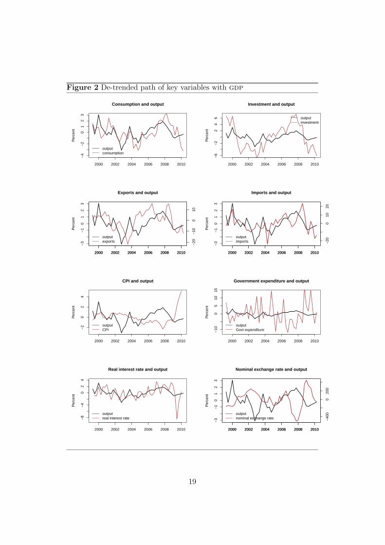
Figure 2 De-trended path of key variables with gdp

Consumption and output

Per

cent

2000 2002 2004 2006 2008 2010

−4

−2

01

23

outputconsumption

Investment and output

Per

cent

2000 2002 2004 2006 2008 2010

−6

−2

24

6 outputinvestment

Exports and output

Per

cent

2000 2002 2004 2006 2008 2010

−3

−1

01

23

2000 2002 2004 2006 2008 2010

−20

−10

010

outputexports

Imports and output

Per

cent

2000 2002 2004 2006 2008 2010

−3

−1

01

23

2000 2002 2004 2006 2008 2010

−20

010

20

outputimports

CPI and output

Per

cent

2000 2002 2004 2006 2008 2010

−2

02

4

outputCPI

Government expenditure and output

Per

cent

2000 2002 2004 2006 2008 2010

−10

05

1015

outputGovt expenditure

Real interest rate and output

Per

cent

2000 2002 2004 2006 2008 2010

−8

−4

02

4

outputreal interest rate

Nominal exchange rate and output

Per

cent

2000 2002 2004 2006 2008 2010

−3

−1

01

23

2000 2002 2004 2006 2008 2010

−40

00

200

outputnominal exchange rate

19

Table 5 Business cycle stylised facts using quarterly data (1999 Q2-2010Q2)

Std. Rel. std. Cont. Persistencedev. dev. corr.

Real gdp 1.18 1.00 1.00 0.73Private Consumption 1.54 1.31 0.51 0.67Investment 4.08 3.43 0.69 0.80cpi 1.30 1.09 -0.29 0.70Exports 8.79 7.40 0.31 0.77Imports 8.93 7.52 0.45 0.54Govt expenditure 6.69 5.53 -0.35 0.005Net exports 1.24 1.04 -0.15 0.45Real interest rate 2.11 1.77 0.38 0.372Nominal exchange rate 4.61 3.88 -0.54 0.82

Volatility : Table 5 shows private consumption as more volatile than output.This is similar to the finding for other developing economies. In general, con-sumption is 40 percent more volatile than income in developing economies.Conversely, in developed economies the ratio is sightly less than one on av-erage (Aguiar and Gopinath, 2007). Table 5 reports the relative volatility ofprivate consumption for India as 1.31.

Prices are also more volatile than output. Again, this is consistent with thefindings for developing economies. In Latin American countries, prices aresix times more volatile than output (Male, 2010). The relative volatility ofprice level for India is 1.09

Exports and Imports exhibit significant volatilities. Higher export and im-port volatilities can also be seen for developed economies, though the extentof volatility is lower. For India, the relative volatility of exports and importsare 7.40 and 7.52 respectively. Net exports are also found to be more volatilethan output.

Consistent with the business cycle facts for developing economies, govern-ment expenditure is more volatile than output. The relative volatility ofgovernment expenditure is 5.53. Thus on volatility, our business cycle fea-tures resemble those of developing economies.

Co-Movement : Table 5 shows investment as significantly pro-cyclical. Thecontemporaneous correlation of investment with output is 0.69. The strongcorrelation between investment and output for India provides evidence for agrowing resemblance between India and advanced economies business cycles.This is consistent with the results from annual data.

20

Table 5 shows imports as pro-cyclical, while exports as mildly pro-cyclical.Again, this feature indicates resemblance between Indian and advanced economiesbusiness cycle facts.

For fiscal policy to play a stabilising role in an economy, government expen-diture should be counter-cyclical. A significant difference between the annualand quarterly data analysis pertains to the correlation of government expen-diture with output. For the annual analysis, the relation is counter-cyclical,though not significant. With the quarterly analysis, which pertains to recentdata, we report a significant counter-cyclical relation between governmentexpenditure and output. The correlation coefficient is -0.35. Crucially, thisis similar to the findings for developed economies.

Also consistent with the results of the annual post-reform period, nominalexchange rate is found to be counter-cyclical.

Persistence11 A central issue in business cycle research is the nature of per-sistence in output fluctuations. Table 5 shows persistent output fluctuationsfor the Indian business cycle. The magnitude of persistence is however lowercompared to those of developed economies. Male (2010) finds the averagepersistence for developed economies to be 0.84 and for developing economiesto be 0.59. The persistence of output for India is higher than the devel-oping economies average figure. The persistence is even higher at 0.84 ifnon-agricultural gdp is taken as the aggregate measure of business cycleactivity. Price levels are also significantly persistent. Significant price persis-tence justifies the use of theoretical models with staggered prices and wagesfor the modeling of developing and emerging market business cycles. Othervariables in Table 5 are also found to be significantly persistent (with theexception of Government expenditure and real interest rate).

In summary, the results of the quarterly data analysis broadly confirm thefindings of the post-reform period using annual data. The findings supportthat the Indian economy is in a transition phase. While on volatility, thebusiness cycle features resemble those of developing economies, the correla-tion results show growing similarity with the advanced economies businesscycle.

11The results on persistence are added in quarterly data analysis.

21

7.2 An Alternative Detrending Method

As another sensitivity measure, we check the robustness of our annual resultsto the choice of the de-trending technique. Following (Stock and Watson,1999; Agenor et al., 2000) we use the Baxter-King to derive the businesscycle properties of our macroeconomic variables. Baxter-King filter belongto the category of band-pass filters that extract data corresponding to thechosen frequency components. We are interested in extracting the businesscycle components. In line with the NBER definition, the business cycleperiodicity is defined as those ranging between 8 to 32 quarters.

Table 6 reports the results with the cyclical components derived from theBaxter-King filter. The results are broadly consistent with those corre-sponding to the Hodrick-Prescott filter. Output volatility shows a declinein the post-reform period. On correlation, the results are broadly the same.Investment becomes pro-cyclical in the post-reform period. Exports is in-significantly pro-cyclical while the cyclicality of imports is significant. Sinceexports is acyclical and imports are pro-cyclical, net exports are found tobe counter-cyclical. Similar to the findings with the Hodrick-Prescott filter,nominal exchange rate becomes counter-cyclical in the post-reform period,though the level of significance varies.

There are some notable differences in the results related to volatility. Thisarises due to differences in the properties of the two filters. While the Baxter-King filter belongs to the category of band-pass filters that remove slowmoving components and high frequency noise, the Hodrick-Prescott filter isan approximation to a high-pass filter that removes the trend but passes highfrequency components in the cyclical part. The Baxter-King filter, howevertends to underestimate the cyclical component. (Rand and Tarp, 2002)12.As an example, in contrast to the findings of the Hodrick-Prescott filter, theabsolute volatility of private consumption declines in the post-reform period,when the Baxter-King filter is used to de-trend the variables. The statisticaltesting procedure shows that the difference in correlations is close to the cut-off value of 1.96, even though it is not as strong as with the Hodrick-Prescottfilter.

12For a detailed comparison of the filtering procedure of Hodrick-Prescott and Baxter-King, refer to (Baxter and King, 1999)

22

Table 6 Business cycle statistics for the Indian economy using annual data:Pre and post reform period (with Baxter-King filter)

Pre-reform period (1950-1991) Post-reform period (1992-2009)

Std. Rel. Cont. Std. Rel. Cont.dev. std. dev. cor. dev. std. dev. cor.

Real gdp 1.94 1.00 1.00 0.95 1.00 1.00Pvt. Cons. 1.59 0.81 0.86 1.05 1.10 0.84Investment 3.49 1.79 0.22 3.12 3.26 0.60cpi 4.29 2.20 0.28 1.51 1.58 0.28Exports 5.99 3.07 -0.03 6.08 6.35 0.36Imports 8.76 4.49 -0.06 6.15 6.42 0.47Govt expenditure 6.39 3.10 -0.17 3.73 3.90 -0.44Net exports 0.68 0.34 0.08 0.81 0.84 -0.26Nominal exchange rate 4.34 2.23 0.05 2.17 2.27 -0.17

7.3 Redefining the Sample Period

Finally, we check the robustness of our results to a change in the sampleperiod. To maintain uniformity in sample size we redefine the pre-reformperiod as starting from 1971.

Table 7 Business cycle statistics for the Indian economy using annual data:Pre (1971-1991) and post reform period

Pre-reform period (1971-1991) Post-reform period (1992-2009)

Std. Rel. Cont. Std. Rel. Cont.dev. std. dev. cor. dev. std. dev. cor.

Real gdp 2.24 1.00 1.00 1.78 1.00 1.00Pvt. Cons. 1.94 0.86 0.69 1.87 1.05 0.89Investment 3.55 1.57 0.50 5.10 2.85 0.77cpi 5.96 2.64 -0.16 3.49 1.95 0.29Exports 6.00 2.66 0.10 7.71 4.31 0.33Imports 8.71 3.87 -0.10 9.61 5.38 0.70Govt expenditure 5.62 2.62 0.50 4.60 2.58 -0.26Net exports 0.8 0.3 0.12 1.1 0.65 -0.69Nominal exchange rate 5.54 2.46 0.40 5.35 3.00 -0.48

Table 7 reports business cycle facts when the pre-reform period is defined asstarting from 1971. The broad stylised facts remain the same. On correlation,our results remain the same as reported in Table 3. Investment and importsbecome highly pro-cyclical, while net exports and nominal exchange rate turn

23

counter-cyclical in the post-reform period. On volatility, we get a mixedpicture. While aggregate gdp is highly volatile at 2.24 in the pre-reformperiod, it falls to 1.78 in the post-reform period. Other variables, with theexception of investment, exports, imports and net exports also show a fall involatility from the pre to post reform period.

8 Conclusion

Documenting business cycle stylised facts forms the foundation of quantita-tive general equilibrium models either in the RBC or DSGE tradition. Sucha study assumes greater relevance in the context of an economy like Indiawhich has undergone significant transformation since 1991. The industrialsector has been freed from capacity controls, import duties have been re-duced and a reasonably conducive environment towards the global economyhas evolved over the last few years. The novel aspect of this paper is topresent a comprehensive set of stylized facts governing an economy in tran-sition. We locate facts about Indian business cycles in the context of otherindustrial economies, as well as other emerging and developing countries.

Our main findings are as follows:

• Output volatility, as measured by the percentage standard deviation ofthe filtered cyclical component of gdp is considerably reduced in thepost-reform period.

• Consistent with the business cycle facts for developed economies, in-vestment becomes highly pro-cyclical in the post-reform period.

• Imports become highly pro-cyclical in the post-reform period.

• Net exports and nominal exchange rate become counter-cyclical in thepost-reform period.

• The quarterly data analysis that focuses only on recent data showsgovernment expenditure to be counter-cyclical. This feature is indica-tive of the growing resemblance between the Indian and the advancedeconomies business cycle.

This kind of study holds relevance not just for India, but for any economythat undergoes transition. An important finding is that for DSGE models toeffectively incorporate the features of an economy in transition, recent datashould be taken.

24

Future work can use the findings of this paper to assess the extent to whichDSGE models, starting with the simplest RBC model through to New-Keynesian models with labour markets and financial frictions introduced instages, can explain business cycle fluctuations in India. Both closed andopen economy models can be examined. Comparisons with a representativedeveloped economy, say the US, can then be made. Proceeding in this way,one will be able to assess the relative importance of various frictions in driv-ing aggregate fluctuations in India. Another avenue for future work relatesto (Lucas, 1987), which pointed out that the welfare gains from eliminatingbusiness cycle fluctuations in the standard RBC model are small, and dwarfedby the gains from increased growth. While adding New Keynesian frictionssignificantly increases the gains from stabilization policy, they still remainsmall compared to the welfare gains from increased growth. However, thereis relatively little work introducing long-run growth into DSGE models, andexploring the relationship between volatility and endogenous growth. Thistakes particular importance for India which has moved to a higher growthpath in recent years, with the attendant decline in macroeconomic volatility,as documented in this paper.

25

References

Agenor P, McDermott C, Prasad E (2000). “Macroeconomic fluctuations in devel-oping countries: Some stylised facts.” The World Bank Economic Review.

Aghion P, Angeletos G, Banerjee A, Manova K (2010). “Volatility and growth:Credit constraints and the composition of investment.” Journal of MonetaryEconomics, 57(3), 246–265. ISSN 0304-3932.

Aghion P, Bacchetta P, Banerjee A (2004). “Financial development and the insta-bility of open economies.” Journal of Monetary Economics, 51, 1077–1106.

Aguiar M, Gopinath G (2007). “Emerging market business cycles: The cycle isthe trend.” Journal of Political Economy, 115(1).

Alper C (2002). “Business cycles, excess volatility, and capital flows: Evidencefrom Mexico and Turkey.” Emerging Markets Finance & Trade, pp. 25–58.ISSN 1540-496X.

Ambler S, Cardia E, Zimmermann C (2004). “International business cycles? Whatare the facts?” Journal of Monetary Economics.

Apergis N (1996). “The cyclical behaviour of prices: Evidence from seven devel-oping countries.” The Developing Economies.

Backus D, Kehoe P (1992). “International evidence on the historical propertiesof business cycles.” The American Economic Review, 82(4), 864–888. ISSN0002-8282.

Batini N, Gabriel V, Levine P, Pearlman J (2010). “A floating versus managedexchange rate regime in a DSGE model of India.” Department of Economics,Surrey University, Discussion Papers.

Baxter M, King R (1999). “Measuring business cycles: approximate band-passfilters for economic time series.” Review of Economics and Statistics, 81(4),575–593. ISSN 0034-6535.

Bjornland H (2000). “Detrending methods and stylized facts of business cycles inNorway- an international comparison.” Empirical Economics.

Boshoff W (December, 2010). “Band-pass filters and business cycle analysis: High-frequency and medium-term deviation cycles in South Africa and what theymeasure .” Universeteit Stellenbosch University, Working Paper, 200.

Burns A, Mitchell W (1946). “Measuring business cycles.” NBER Books.

Burnside C (1998). “Detrending and business cycle facts: A comment.” Journalof Monetary Economics.

26

Calderon C, Fuentes R (2006). “Complementarities between institutions and open-ness in economic development: Evidence for a panel of countries.” Cuadernosde economıa, 43, 49–80. ISSN 0717-6821.

Calderon C, Fuentes R (2010). “Characterising the business cycles of emergingeconomies.” Policy Research Working Paper, The World Bank.

Calvo G (1998). “Capital flows and capital-market crises: the simple economics ofsudden stops.” Journal of Applied Economics, 1(1), 35–54.

Canova F (1998). “Detrending and business cycle facts.” Journal of MonetaryEconomics.

Chadha B, Prasad E (1994). “Are prices countercyclical?: Evidence from the G-7.”Journal of Monetary Economics, pp. 239–254.

Chakraborty S (2008). “Indian economic growth.” UNU-WIDER Research PaperNo. 2008/67.

Chari V, Kehoe P, McGrattan E (2007). “Business cycle accounting.” Economet-rica, 75(3), 781–836. ISSN 1468-0262.

Den Reijer A (2002). “International business cycle indicators, measurement andforecasting.” De Nederlandsche Bank Research Memorandum.

Dua P, Banerji A (2001). “An indicator approach to business and growth ratecycles: The case of India.” Indian Economic Review, 36, 55–78.

Gabriel V, Levine P, Pearlman J, Yang B (2010). “An estimated DSGE model ofthe Indian economy.” Department of Economics, Surrey University, DiscussionPapers.

Garcia-Cicco J, Pancrazi R, Uribe M (2010). “Real business cycles in emergingcountries?” The American Economic Review, pp. 2510–2531.

Hodrick R, Prescott E (1997). “Postwar US business cycles: An empirical investi-gation.” Journal of Money, Credit & Banking, 29(1).

Iacobucci A, Noullez A (2005). “A frequency selective filter for short-length timeseries.” Computational economics, 25(1), 75–102. ISSN 0927-7099.

Jayaram S, Patnaik I, Shah A (2009). “Examining the decoupling hypothesis forIndia.” Economic and Political Weekly, XLIV(44), 109–116.

Kaldor N (1957). “A model of economic growth.” The Economic Journal, 67(268),591–624. ISSN 0013-0133.

King R, Rebelo S (1999). “Resuscitating real business cycles.” Handbook of macroe-conomics, 1, 927–1007.

27

Kose M, Otrok C, Whiteman C (2003). “International business cycles: World,region, and country-specific factors.” American Economic Review, 93(4), 1216–1239. ISSN 0002-8282.

Kydland F, Prescott E (1990). “Business cycles: Real facts and a monetary myth.”Real business cycles: a reader, p. 383.

Loayza N, Ranciere R, Serven L, Ventura J (2007). “Macroeconomic volatility andwelfare in developing countries: An introduction.” The World Bank EconomicReview, 21(3), 343. ISSN 0258-6770.

Lucas R (1987). Models of business cycles. Basil Blackwell New York. ISBN0631147918.

Lucas RJ (1977). “Understanding business cycles.” In “Carnegie-Rochester Con-ference Series on Public Policy,” .

Male R (2010). “Developing country business cycle: Revisiting the stylised facts.”Queen Mary, University of London, Working Paper No. 664.

Neumeyer P, Perri F (2005). “Business cycles in emerging economies: The role ofinterest rates.” Journal of Monetary Economics.

Patnaik I, Sharma R (2002). “Business cycles in the Indian economy.” MARGIN-NEW DELHI-, 35, 71–80. ISSN 0025-2921.

Ramey G, Ramey VA (1995). “Cross-country evidence on the link between volatil-ity and growth.” The American Economic Review, 85(5), 1138–1151.

Rand J, Tarp F (2002). “Business cycles in developing countries: Are they differ-ent?” World Development, 30(12), 2071–2088. ISSN 0305-750X.

Rebelo S (2005). “Business cycles.” Annals of Economics and Finance, 6, 229–250.

Shah A (2008). “New issues in macroeconomic policy.” Business Standard India,pp. 26–54.

Shah A, Patnaik I (2010). “Stabilising the Indian business cycle.” India on growthturnpike: Essays in honour of Vijay L. Kelkar, pp. 136–154.

Stock J, Watson M (1999). “Business cycle fluctuations in US macroeconomic timeseries.” Handbook of Macroeconomics, 1, 3–64. ISSN 1574-0048.

Uribe M, Yue V (2006). “Country spreads and emerging markets: Who driveswhom?” Journal of International Economics, pp. 6–36.

28

A Data Definition and Sources

Variable Definition Source

Gross domestic product gdp is a measure of the volume of all National Accountsgoods and services produced by an Statisticseconomy during a given period of time.gdp is expressed at 2004-05 pricesand chained backwards to 1999-2000 prices.The variable is expressed at factor cost

Private consumption The Private final consumption expenditure National Accountsis defined as the expenditure incurred Statisticsby the resident householdson final consumption of goodsand services, whether made withinor outside economic territory.The variable is expressed at 2004-05 pricesand chained backwards to 1999-2000 prices

Gross fixed capital formation Gross fixed capital formation refers National Accountsto the aggregate of gross additions to Statisticsfixed assets and increase in inventories.The variable is expressed at 2004-05 pricesand chained backwards till 1999-2000 prices

Exports Exports of goods and services, rebased at National Accounts1999-2000 prices. Statistics

Imports Imports of goods and services, rebased at National Accounts1999-2000 prices. Statistics.

Net exports Exports - Imports divided by gdp at constantprices

Consumer prices Consumer Price Index for Industrial Labour Bureau,Workers measured at 2001 prices Ministry of Labour

and Employment.Government expenditure Total expenditure of the Central Government Budget documents,

on revenue and capital accounts Government of IndiaReal interest rate 91-day treasury bill rate Reserve Bank

deflated by of Indiacpi inflation

Nominal exchange rate Nominal rupee-dollar Reserve Bankexchange rate of India.

29