Has Globalization Changed the Phillips Curve? Firm … · Has Globalization Changed the Phillips...

Has Globalization Changed the Phillips Curve?Firm-Level Evidence on the Effect of

Activity on Prices∗

Eugenio GaiottiEconomic Outlook and Monetary Policy Department, Bank of Italy

The flattening of the Phillips curve observed in the indus-trial countries has been attributed to globalization, in contrastwith the traditional explanation centered on monetary pol-icy credibility. The empirical literature is not conclusive. Thispaper argues that recourse to micro data is needed to iden-tify whether changes in the slope of the Phillips curve arestructural. Taking advantage of a unique data set includingabout 2,000 Italian firms, the paper tests whether a changein the link between capacity utilization and prices is con-firmed at the company level and whether it is concentratedamong those firms that are more exposed to foreign competi-tion. The answer is either inconclusive or negative in all cases.The results do not lend support to the view that the flatteningof the Phillips curve is due to globalization.

JEL Codes: E31, E52, E58.

1. Introduction

A widespread flattening of the Phillips curve has taken place inrecent years. In virtually all the advanced economies, the responseof inflation to a variety of measures of cyclical slack (such asthe unemployment gap, the output gap, or the degree of capacity

∗I thank Herve Le Bihan for discussion of a previous version of this paperand three anonymous referees. I am also indebted to Paolo Angelini, MatteoBugamelli, Silvia Fabiani, Domenico Marchetti, Alessandro Secchi, and all theparticipants in the 2009 IJCB annual conference in Paris for comments and sug-gestions on previous versions of this paper. The usual disclaimer applies. E-mail:[email protected].

51

52 International Journal of Central Banking March 2010

utilization) has steadily decreased since the 1980s.1 There has beenmuch discussion on how monetary policymakers should react to thisfinding: does it indicate that a structural change in the trade-offbetween output and inflation variability took place, or is it simplyan endogenous sign of monetary policy success?

An influential argument, advanced by Borio and Filardo (2007),as well as by others, draws a link between the flattening of thePhillips curve and the spread of globalization or, more precisely,the stronger competitive pressures from emerging countries, notablyfrom Asia, unleashed by the increasing openness of the internationaleconomy.2 There are various versions of this story, the common ele-ment being that globalization has changed the price-setting behaviorof individual firms. According to this view, foreign competition hasreduced the pricing power of domestic corporations, limiting theirability to raise prices during booms in response to transitory domes-tic cost or demand pressures; the prices of items produced at homeare increasingly determined by foreign demand and supply factors,rather than domestic ones; and on the labor market, the threat ofoutsourcing to cheaper labor countries disciplines wages, keepingthem low and less responsive to increases in demand.3

According to this “globe-centric” view, global, rather thandomestic, slack is a major driving force of domestic inflation rates,and a flatter Phillips curve is a structural feature of advancedeconomies. If true, this would have far-reaching implications for theconduct of monetary policy. The most obvious is that monetary pol-icy would have more leeway to fine-tune domestic activity, with lessneed to worry about inflation variability. According to Bean (2006a,2006b), it implies that policy errors would not show up in large move-ments of inflation away from the target, and at the same time thatvariations in aggregate demand are a less effective means of con-trolling inflation. Woodford (2007) argues that central banks maylose incentive to control inflation if they perceive a flatter trade-offbetween output expansion and inflation.

1See International Monetary Fund (2006), Kohn (2006), and Pain, Koske, andSollie (2006).

2See also Bank for International Settlements (2006).3Bean (2006a, 2006b).

Vol. 6 No. 1 Has Globalization Changed the Phillips Curve? 53

However, there is controversy. According to Rogoff (2006), anincrease in international competition could in principle steepen,rather than flatten, the Phillips curve: firms revise prices morefrequently, as the cost of keeping prices fixed at the wrong levelincreases.4 Ball (2006) argues that, even with greater internationalcompetition, marginal costs still depend on the firm’s own outputlevels. Woodford (2007), based on a two-country New Keynesianmodel, shows that even in an open economy and with a singleworld market for labor, the aggregate supply relation still connectsdomestic inflation with domestic economic activity.

A long-standing tradition in economic analysis, since the sem-inal contributions by Friedman, Phelps, and Lucas, emphasizesthe pitfalls of treating estimated Phillips curves as structural rela-tionships. The traditional line of argument links the flattening ofPhillips curves to the very success of monetary policy in stabilizingactual and expected inflation. Negative correlation between “sacri-fice ratios” and the average inflation rate may reflect an endogenousadjustment of the degree of price stickiness to lower inflation,5 or achange in the way inflation expectations are formed under a morecredible policy regime; treating these endogenous and reversiblechanges of the output-inflation trade-off as if they were structuralmay lead to recurrent policy mistakes, generated by the very suc-cess obtained in the past. Sargent, Williams, and Zha (2006) haveshown that this may be the case when short-sighted policymakersrecursively estimate a non-expectational, backward-looking Phillipscurve and update their beliefs and policies accordingly.

Assessing whether the change in the slope of the Phillips curveis a structural consequence of globalization or just an endogenousby-product of the success of monetary policy is therefore extremelyrelevant. However, the empirical literature is inconclusive: althoughthey use a similar approach, the International Monetary Fund (2006)finds that globalization has reduced the sensitivity of inflation todomestic capacity, while Ball (2006) and Ihrig et al. (2007) find

4A similar conclusion was reached by Romer (1993) based on a different argu-ment: sacrifice ratios should be smaller in open economies, since an expansionarymonetary policy has larger effects on inflation via the exchange rate, and smallereffects on output, via the higher price of imported inputs.

5Ball, Mankiw, and Romer (1988).


little or no effect.6 The evidence presented is almost entirely basedon the estimation of reduced-form relationships and on macroeco-nomic data. The problems raised by this approach hinge on thelack of cross-sectional variability in the data and on the difficulty ofproperly accounting for inflation expectations. There is an emergingconsensus that more disaggregated information is needed.7

The empirical strategy followed in this paper is to exploit micro-economic evidence, making extensive recourse to individual data andexploiting the variability in firm characteristics, to better identifythe underlying structural relationship and to examine observableimplications overlooked by the macroeconomic literature. This paperexploits a unique data set, including almost twenty years of annualinformation on individual firms’ pricing and capacity utilization, aswell as on various aspects of their exposure to globalization. Theavailability of firm-level information makes it possible to better con-trol for aggregate effects, such as changes in inflation expectations,avoiding the problems typical of aggregate estimates of the Phillipscurve. It also makes it possible to test for some observable implica-tions of the hypotheses discussed above, e.g., the fact that the changein the sensitivity of prices to capacity utilization is more pronouncedfor those firms which are more directly exposed to the competitionof emerging countries.

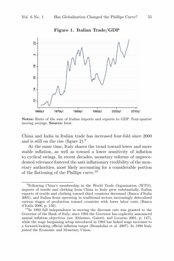
Italy is also an appropriate case to study. Given its traditionalspecialization in low- and medium-technology production, like tex-tiles and clothing, the Italian economy has been particularly affectedby increased competition from emerging countries, notably Asianones.8 While the degree of trade openness of the Italian economyhas been slightly rising (figure 1), the change in the composition oftrade since the beginning of this century is startling; the share of

6Previous literature on the link between openness and sacrifice ratios also pro-duced mixed results. See Temple (2002), Daniels, Nourzad, and Vanhoose (2005),and Razin and Loungani (2005).

7This is also pointed out by Borio and Filardo (2007).8Italian industry is specialized in medium-to-low technology sectors (textiles

and clothing, leather and footwear) that are particularly vulnerable to competi-tion from newly industrialized countries. In 2000–01 only 13 percent of Italianexports was in high-tech sectors, while 44 percent was in low-tech sectors, mostlytextile and clothing; the same figures for the euro area were 30 percent and 21percent (European Central Bank 2005).


Figure 1. Italian Trade/GDP

Notes: Ratio of the sum of Italian imports and exports to GDP. Four-quartermoving average. Source: Istat.

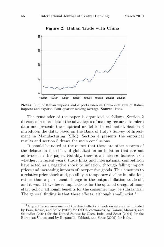
China and India in Italian trade has increased four-fold since 2000and is still on the rise (figure 2).9

At the same time, Italy shares the trend toward lower and morestable inflation, as well as toward a lower sensitivity of inflationto cyclical swings. In recent decades, monetary reforms of unprece-dented relevance fostered the anti-inflationary credibility of the mon-etary authorities, most likely accounting for a considerable portionof the flattening of the Phillips curve.10

9Following China’s membership in the World Trade Organization (WTO),imports of textile and clothing from China to Italy grew substantially, Italianexports of textile and clothing toward third countries decreased (Banca d’Italia2005), and Italian firms operating in traditional sectors increasingly delocalizedvarious stages of production toward countries with lower labor costs (Bancad’Italia 2006, p. 156).

10In 1992 full independence in moving the discount rate was granted to theGovernor of the Bank of Italy; since 1994 the Governor has explicitly announcedannual inflation objectives (see Altissimo, Gaiotti, and Locarno 2001, p. 147),while the wage bargaining setup introduced in 1993 has linked wage increases toa forward-looking official inflation target (Brandolini et al. 2007). In 1998 Italyjoined the Economic and Monetary Union.


Figure 2. Italian Trade with China

Notes: Sum of Italian imports and exports vis-a-vis China over sum of Italianimports and exports. Four-quarter moving average. Source: Istat.

The remainder of the paper is organized as follows. Section 2discusses in more detail the advantages of making recourse to microdata and presents the empirical model to be estimated. Section 3introduces the data, based on the Bank of Italy’s Survey of Invest-ment in Manufacturing (SIM). Section 4 presents the empiricalresults and section 5 draws the main conclusions.

It should be noted at the outset that there are other aspects ofthe debate on the effect of globalization on inflation that are notaddressed in this paper. Notably, there is an intense discussion onwhether, in recent years, trade links and international competitionhave acted as a negative shock to inflation, through falling importprices and increasing imports of inexpensive goods. This amounts toa relative price shock and, possibly, a temporary decline in inflation,rather than a permanent change in the output-inflation trade-off,and it would have fewer implications for the optimal design of mon-etary policy, although benefits for the consumer may be substantial.The general finding is that these effects, although small, exist.11

11A quantitative assessment of the direct effects of trade on inflation is providedby Pain, Koske, and Sollie (2006) for OECD economies; by Kamin, Marazzi, andSchindler (2004) for the United States; by Chen, Imbs, and Scott (2004) for theEuropean Union; and by Bugamelli, Fabiani, and Sette (2009) for Italy.


2. The Empirical Approach

The existing empirical literature is based on the aggregate specifi-cation:12

πt = πet+1 + α0

(yt − y∗

t

)+ α1Tt

(yt − y∗

t

)+ ηt, (1)

where πt stands for inflation at time t, πet+1 stands for expected

inflation, yt stands for output at time t, and y∗t stands for poten-

tial output at time t. To measure the impact of globalization on theslope α0, the output gap is interacted with the trade/GDP ratio Tt.

Substantial econometric issues arise in the empirical implemen-tation of (1). First, πe

t+1 is difficult to measure. Ball (2006) showsthat the results are not robust to the choice of a proxy; in addition,the almost universal practice of adopting a backward-looking vari-able, like lagged inflation, is subject to the Sargent, Williams, andZha (2006) critique. The low variance in πt,π

et+1 during the “Great

Moderation” makes (1) hard to estimate efficiently. Finally, Tt lackscross-sectional variability and it could be spuriously correlated withπe

t+1.This paper replicates equation (1) at the firm level. Focusing on

individual data makes it possible to control for inflation expecta-tions in a straightforward way, to exploit cross-sectional variability,and to use information on each firm’s exposure to international com-petition. The effects of globalization are likely to be quite differentdepending on firms’ characteristics, as they operate through firm-specific channels: marginal costs may have become less sensitive tothe business cycle, as the threat of locating activities offshore inChina, India, or Eastern Europe diminishes the power of workers toclaim higher wages (via overtime compensation or production pre-mia) at a time of increasing pressure on labor utilization by the firm;increased competition from emerging countries may have decreasedthe scope of a firm to move its prices in response to a cyclical rise inmarginal costs, affecting the cyclical behavior of its profit margins.

We start from the definition of the change in prices by firm i:

Δpi,t = Δmci,t + Δμi,t, (2)

12Equation (1) is from Ball (2006). The International Monetary Fund (2006)and Ihrig et al. (2007) follow a similar approach.


where pi,t is the price set by firm i in year t, mci,t stands for mar-ginal labor costs, and μi,t stands for the markup (all variables arein logs).13 We adopt the assumption that all prices are adjustedwithin a single year. While simplifying the notation, such an assump-tion is not unreasonable in light of the existing evidence on pricerevisions.14

To derive a firm-level supply function, two features are thentaken into account: marginal labor costs are affected by the degreeof capacity utilization; adjustments in markups may compensate forpart of the cyclical movements in marginal costs. It is convenient toexpress the change in marginal labor cost as the sum of the changein the national contractual wage, wC

t , and of a firm-specific wagecomponent, wF

i,t, less the change in labor productivity δi,t:

Δmci,t = ΔwCt + ΔwF

i,t − Δδi,t. (3)

In the Italian labor market setup,15 national contractual wageswC

t incorporate both a forward-looking and a backward-lookingexpectations term: ΔwC

t = aπt|t−1 +(1−a)πt+1|t +ε′t. The firm also

faces a firm-specific upward-sloping supply curve for labor, as work-ers demand a higher wage to supply extra hours or enjoy overtimepremia written into labor contracts:16 the growth in the firm-levelwage component is a positive function of the deviation of activityyi,t from its steady-state level y∗

i,t: ΔwFi,t = γ(yi,t − y∗

i ) + ε′′i,t.

17

Δmci,t = [a′πt|t−1 + (1 − a′)πt+1|t] + γ(yi,t − y∗

i,t

)+ εi,t (4)

13Here we abstract from the cost of intermediate inputs, for the sake of nota-tional simplicity. It is included later.

14In Italy firms are found to revise prices on average every ten to eleven monthsbased on both micro quantitative data (Fabiani et al. 2006) and surveys (Fabiani,Gattulli, and Sabbatini 2007).

15National wage agreements are meant to safeguard purchasing power, based onthe official forecast for inflation over the contract period (two years) at the timethe contract was signed; productivity gains and real wage increases are mostlyleft to firm-level agreements (Brandolini et al. 2007).

16See Rotemberg and Woodford (1999).17Under the assumption of firm-specific capital, fixed in the short run (Altig

et al. 2005), labor productivity may also decrease with the deviation of activityfrom its steady-state level: Δδi,t = −β(yi,t −y∗

i,i)+ν′′i,t. This effect is not included

here for the sake of simplicity; it would not change the results in any substantialway.


A link between markups and cyclical conditions may derivefrom the existence of customer markets. An asymmetric reactionof demand to price increases and decreases may follow from the ideathat the consumer is subject to search costs due to imperfect infor-mation on other firms’ prices.18 Ball and Romer (1990) show thatin this case the desired markup is a function of the firm’s relativeprice, μi,t = μi − k(pi,t − pt|t−1) + τi,t, and therefore partly absorbssome of the cyclical movements in nominal marginal costs:

Δμi,t = −(

k

1 + k

)Δ

(wF

i,t − δi,t

)+ ϕi.t. (5)

The individual firm’s pricing equation is then

Δpi,t = [aπt|t−1 + (1 − a)πt+1|t] +(

γ

1 + k

) (yi,t − y∗

i,t

)+ ηi,t. (6)

We interpret the arguments advanced in support of the “global-ization and the Phillips curve” hypothesis as implying that, as aneffect of delocalization, the slope of firm-specific labor supply curves,γ, decreases, since firms are able to outsource production in timesof increasing demand. In addition, we interpret it as also implyingthat, since firms face new foreign competitors and risk losing theircustomers if they increase prices, k increases and desired markupsabsorb a larger part of the cyclical movements in marginal costs.19

As a result, a decrease in γ/(1+k) is the conjecture we want to test.Averaging (6) over firms, an aggregate Phillips curve of the same

form as (1) above could be obtained. However, the estimate of (6)is not affected by the usual problems since it is possible to controlfor inflation expectations, πt+1|t, and to take advantage of cross-firmvariability.

18Rotemberg and Woodford (1999) survey a wide range of models of variabledesired markups, based on variable elasticity of demand, on customer markets(where firms set prices not only to maximize current profits but also to expandtheir customer base in the future), on implicit collusion, and on variable firmentry.

19Ball and Romer (1990) show that such an implication requires the assump-tion that, if prices are kept at their current level, most buyers remain with theiroriginal sellers.


We write an augmented version of (6):

Δpi,t = si + dt + a1CUi,t + b1(λiΔWNAT

t

)+ b2(1 −λi)ΔP INP

t + ηi.t,(7)

where time fixed effects dt control for inflation expectations(πt|t−1, πt+1|t), which are assumed equal across agents. CUi,t is theobserved degree of capacity utilization at firm level, which proxies for(yt − y∗

t ). Individual fixed effects si control, among other things, fora firm-specific steady-state level of capacity utilization, CU∗

i . Twoadditional regressors are included to fully account for price determi-nants: the change in the price of intermediate inputs (ΔP INP

t ) timestheir share over the firm’s variable costs (1 − λi), and the change innational contractual wages (ΔWNAT

t ) times labor’s share over thefirm’s variable costs (λi) (b1 = b2 = 1 is expected).

We first assess whether the observed flattening of the macro-economic Phillips curve can be replicated at the micro level by acorresponding decrease in a1 in (7). This should not be the case ifthe change in the slope observed at the macroeconomic level is onlya statistical artefact due to the dynamics of inflation expectations,a la Sargent, Williams, and Zha (2006).

We then interact CUi,t with firm-specific measures of exposureto globalization (Ti,t):

Δpi,t = si + dt + a1CUi,t + a2Ti,tCUi,t + b1(λiΔWNAT

t

)+ b2(1 − λi)ΔP INP

t + ηi.t. (7a)

We choose Ti,t in several alternative ways: the firm-level shareof export over sales (the closer micro counterpart of (1) above), tosingle out those firms whose pricing power is reduced by exposureto competitive pressures on their export markets; the Asian share inItalian imports of the firm’s (three-digit) type of product, an indi-cator of competitive pressures exerted from low-cost producers onItalian firms’ domestic markets; and a dummy taking value 1 if ina specific year the firm was carrying productive activity abroad, tosingle out those firms who are able to shift production offshore andare therefore less affected by pressures on resource utilization. Theassumption that globalization affected the slope of supply curvesimplies a2 < 0.


A variant of the previous experiment is based on the idea thatthe economically relevant increase in international integration waslargely fostered by a single institutional event, China’s joining theWTO (November 2001); competitive pressures exerted by China aremostly price based and are particularly relevant for Italy’s labor-intensive, low-technology productions. As an interaction variable,we use an aggregate measure of the share of trade with China intoItalian trade (TCt), which starts accelerating in 2001 (figure 2); inaddition, we exploit the information on the firms who declare thattheir competitors are Chinese (identified by a dummy Di) to splitthe sample. We expect a4 < 0.

Δpi,t = si + dt + a1CUi,t + a2TCtCUi,t + b1(λiΔWNAT

t


t + ηi.t + Di

[dt + a3CUi,t + a4TCtCUi,t

+ b3(λiΔWNAT

t


t

](7b)

For these purposes, we need firm-level information on pricechanges and on the degree of capacity utilization. In addition, weneed to find measures of the firms’ exposure to international compe-tition, focusing on export orientation, on foreign penetration in thedomestic market, on the possibility to delocalize production, and onthe presence of foreign competitors.

3. The Data

We obtain data from the Bank of Italy’s annual Survey of Invest-ment in Manufacturing (SIM). The SIM is an open panel of about1,200 firms, which contains specific information on individual Italianmanufacturing firms since 1978.20 During the last two decades, thesurvey has been extensively used to investigate a large number oftopics.21

20Services firms were only recently included in the survey, which is cur-rently known as the Survey of Industrial and Services Firms. See http://www.bancaditalia.it/statistiche/indcamp/indimpser. Each year about 15–20 percentof firms are dropped from the sample due to attrition and are replaced by firmswith comparable characteristics.

21Full references can be found in Gaiotti and Secchi (2006). For recent research,see Bugamelli (2007) and Bugamelli, Fabiani, and Sette (2009).


Data are collected at the beginning of each year, relative to theprevious year, by interviewing a stratified sample of firms with morethan fifty employees (smaller firms have only been included since2003).22 The survey includes information on employment, invest-ment, production, and technical capacity, as well as on specific topicsthat change year by year. Data revision is carried out by officials ofthe Bank of Italy. A special effort is made to keep information asclosely comparable as possible in subsequent years.

A major advantage of SIM is that it contains information on anumber of variables that are not usually available. For our purposes,since 1988, firms have been asked to report the percentage changein the average price of goods sold. The firm-level rate of capacityutilization is also available, as the answer to the question, Whatis the ratio between actual production and the level of productionwhich would be possible by fully using the available capital goodsand without changing labor inputs?

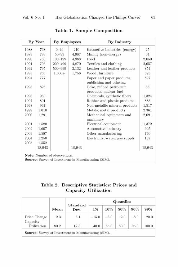
Our complete sample, obtained by dropping all the data pointsfor which information on either price changes or capacity utilizationis missing, covers the period 1988–2005; it includes 18,943 observa-tions and between 800 and 1,600 firms per year (table 1). The averagestay of a firm in the sample is five years. The sample is broadly rep-resentative of the industry composition of the Italian economy; ittends to be slightly biased toward larger firms.

Descriptive statistics on the two main variables are reported intable 2. The average annual price change is around 2 percent; thereis a high degree of variability across firms. As for capacity utiliza-tion, firms on average report that they are using 80 percent of theircapacity; the dispersion of this variable is relatively high, rangingfrom 100 to 40 percent, with a few observations below this value.Capacity utilization is also closely connected to movements of thefirm-specific component of marginal costs.23

22The sample is stratified according to sector (two-digit classification of theItalian National Institute of Statistics, Istat), size (number of employees), andgeographical location (region).

23Simple regressions show that a ten-point increase in capacity utilization (themedian absolute change in our sample) is correlated to an increase in labor com-pensation per capita of about 1 percent, an increase in total costs per unit ofoutput of about 2 percent, and a greater recourse to overtime hours of about 0.1percent of total hours. For details, see the working paper version of this research(Gaiotti 2008).


Table 1. Sample Composition

By Year By Employees By Industry

1988 768 0–49 210 Extractive industries (energy) 251989 799 50–99 4,987 Mining (non-energy) 641990 760 100–199 4,988 Food 2,0501991 795 200–499 4,870 Textiles and clothing 2,6571992 795 500–999 2,132 Leather and leather products 8541993 766 1,000+ 1,756 Wood, furniture 3231994 777 Paper and paper products,

publishing and printing897

1995 828 Coke, refined petroleumproducts, nuclear fuel

53

1996 950 Chemicals, synthetic fibers 1,3241997 891 Rubber and plastic products 8831998 937 Non-metallic mineral products 1,5171999 1,010 Metals, metal products 2,3612000 1,291 Mechanical equipment and

machinery2,691

2001 1,580 Electrical equipment 1,3722002 1,607 Automotive industry 9952003 1,587 Other manufacturing 7402004 1,250 Electricity, water, gas supply 1372005 1,552

18,943 18,943 18,943

Note: Number of observations.Source: Survey of Investment in Manufacturing (SIM).

Table 2. Descriptive Statistics: Prices andCapacity Utilization

StandardDev.

Quantiles

Mean 1% 10% 50% 90% 99%

Price Change 2.3 6.1 −15.0 −3.0 2.0 8.0 20.0Capacity

Utilization 80.2 12.8 40.0 65.0 80.0 95.0 100.0

Source: Survey of Investment in Manufacturing (SIM).


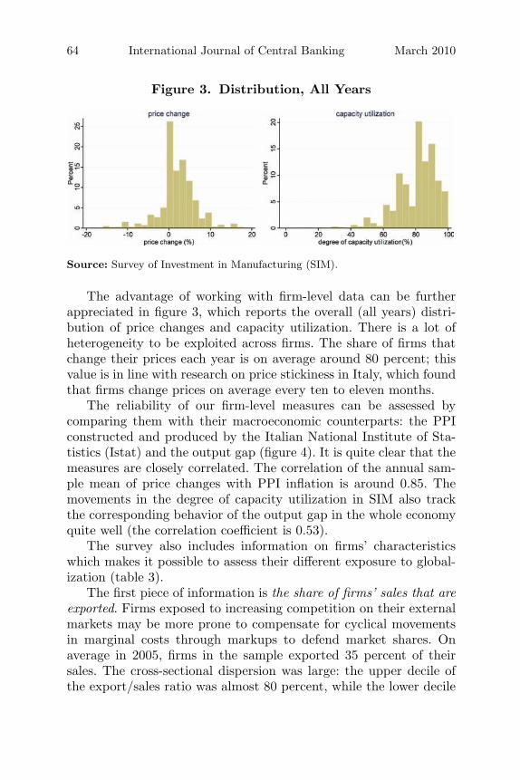
Figure 3. Distribution, All Years


The advantage of working with firm-level data can be furtherappreciated in figure 3, which reports the overall (all years) distri-bution of price changes and capacity utilization. There is a lot ofheterogeneity to be exploited across firms. The share of firms thatchange their prices each year is on average around 80 percent; thisvalue is in line with research on price stickiness in Italy, which foundthat firms change prices on average every ten to eleven months.

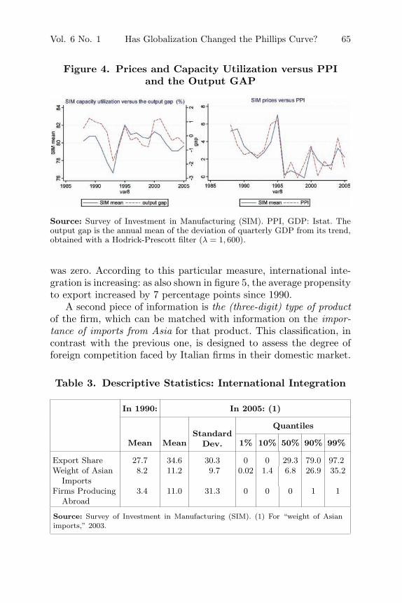
The reliability of our firm-level measures can be assessed bycomparing them with their macroeconomic counterparts: the PPIconstructed and produced by the Italian National Institute of Sta-tistics (Istat) and the output gap (figure 4). It is quite clear that themeasures are closely correlated. The correlation of the annual sam-ple mean of price changes with PPI inflation is around 0.85. Themovements in the degree of capacity utilization in SIM also trackthe corresponding behavior of the output gap in the whole economyquite well (the correlation coefficient is 0.53).

The survey also includes information on firms’ characteristicswhich makes it possible to assess their different exposure to global-ization (table 3).

The first piece of information is the share of firms’ sales that areexported. Firms exposed to increasing competition on their externalmarkets may be more prone to compensate for cyclical movementsin marginal costs through markups to defend market shares. Onaverage in 2005, firms in the sample exported 35 percent of theirsales. The cross-sectional dispersion was large: the upper decile ofthe export/sales ratio was almost 80 percent, while the lower decile


Figure 4. Prices and Capacity Utilization versus PPIand the Output GAP

Source: Survey of Investment in Manufacturing (SIM). PPI, GDP: Istat. Theoutput gap is the annual mean of the deviation of quarterly GDP from its trend,obtained with a Hodrick-Prescott filter (λ = 1, 600).

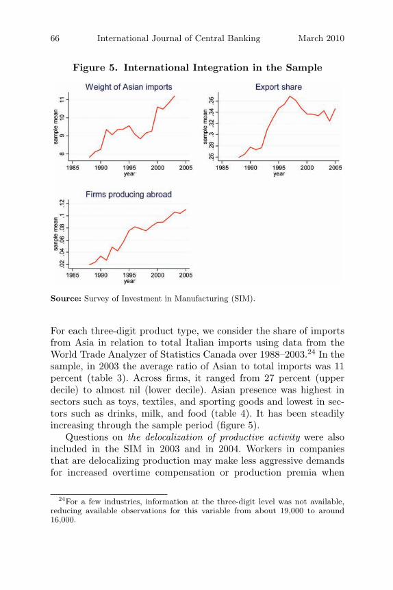
was zero. According to this particular measure, international inte-gration is increasing: as also shown in figure 5, the average propensityto export increased by 7 percentage points since 1990.

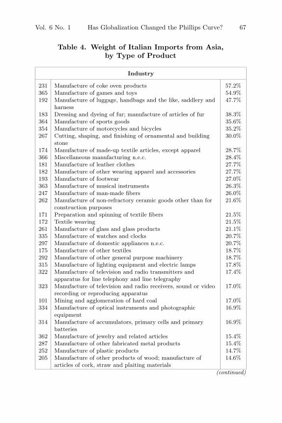
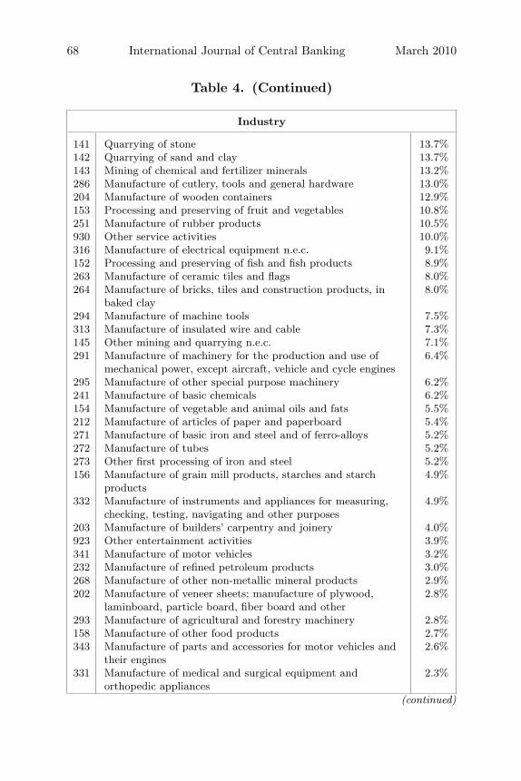
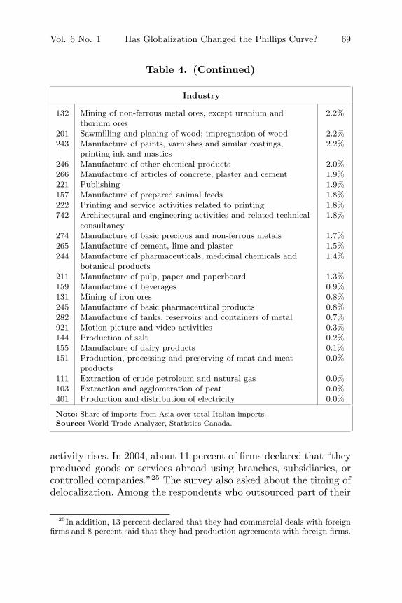
A second piece of information is the (three-digit) type of productof the firm, which can be matched with information on the impor-tance of imports from Asia for that product. This classification, incontrast with the previous one, is designed to assess the degree offoreign competition faced by Italian firms in their domestic market.

Table 3. Descriptive Statistics: International Integration

In 1990: In 2005: (1)

StandardDev.

Quantiles

Mean Mean 1% 10% 50% 90% 99%

Export Share 27.7 34.6 30.3 0 0 29.3 79.0 97.2Weight of Asian

Imports8.2 11.2 9.7 0.02 1.4 6.8 26.9 35.2

Firms ProducingAbroad

3.4 11.0 31.3 0 0 0 1 1

Source: Survey of Investment in Manufacturing (SIM). (1) For “weight of Asianimports,” 2003.


Figure 5. International Integration in the Sample


For each three-digit product type, we consider the share of importsfrom Asia in relation to total Italian imports using data from theWorld Trade Analyzer of Statistics Canada over 1988–2003.24 In thesample, in 2003 the average ratio of Asian to total imports was 11percent (table 3). Across firms, it ranged from 27 percent (upperdecile) to almost nil (lower decile). Asian presence was highest insectors such as toys, textiles, and sporting goods and lowest in sec-tors such as drinks, milk, and food (table 4). It has been steadilyincreasing through the sample period (figure 5).

Questions on the delocalization of productive activity were alsoincluded in the SIM in 2003 and in 2004. Workers in companiesthat are delocalizing production may make less aggressive demandsfor increased overtime compensation or production premia when

24For a few industries, information at the three-digit level was not available,reducing available observations for this variable from about 19,000 to around16,000.


Table 4. Weight of Italian Imports from Asia,by Type of Product

Industry

231 Manufacture of coke oven products 57.2%365 Manufacture of games and toys 54.9%192 Manufacture of luggage, handbags and the like, saddlery and

harness47.7%

183 Dressing and dyeing of fur; manufacture of articles of fur 38.3%364 Manufacture of sports goods 35.6%354 Manufacture of motorcycles and bicycles 35.2%267 Cutting, shaping, and finishing of ornamental and building

stone30.0%

174 Manufacture of made-up textile articles, except apparel 28.7%366 Miscellaneous manufacturing n.e.c. 28.4%181 Manufacture of leather clothes 27.7%182 Manufacture of other wearing apparel and accessories 27.7%193 Manufacture of footwear 27.0%363 Manufacture of musical instruments 26.3%247 Manufacture of man-made fibers 26.0%262 Manufacture of non-refractory ceramic goods other than for

construction purposes21.6%

171 Preparation and spinning of textile fibers 21.5%172 Textile weaving 21.5%261 Manufacture of glass and glass products 21.1%335 Manufacture of watches and clocks 20.7%297 Manufacture of domestic appliances n.e.c. 20.7%175 Manufacture of other textiles 18.7%292 Manufacture of other general purpose machinery 18.7%315 Manufacture of lighting equipment and electric lamps 17.8%322 Manufacture of television and radio transmitters and

apparatus for line telephony and line telegraphy17.4%

323 Manufacture of television and radio receivers, sound or videorecording or reproducing apparatus

17.0%

101 Mining and agglomeration of hard coal 17.0%334 Manufacture of optical instruments and photographic

equipment16.9%

314 Manufacture of accumulators, primary cells and primarybatteries

16.9%

362 Manufacture of jewelry and related articles 15.4%287 Manufacture of other fabricated metal products 15.4%252 Manufacture of plastic products 14.7%205 Manufacture of other products of wood; manufacture of

articles of cork, straw and plaiting materials14.6%

(continued)


Table 4. (Continued)

Industry

141 Quarrying of stone 13.7%142 Quarrying of sand and clay 13.7%143 Mining of chemical and fertilizer minerals 13.2%286 Manufacture of cutlery, tools and general hardware 13.0%204 Manufacture of wooden containers 12.9%153 Processing and preserving of fruit and vegetables 10.8%251 Manufacture of rubber products 10.5%930 Other service activities 10.0%316 Manufacture of electrical equipment n.e.c. 9.1%152 Processing and preserving of fish and fish products 8.9%263 Manufacture of ceramic tiles and flags 8.0%264 Manufacture of bricks, tiles and construction products, in

baked clay8.0%

294 Manufacture of machine tools 7.5%313 Manufacture of insulated wire and cable 7.3%145 Other mining and quarrying n.e.c. 7.1%291 Manufacture of machinery for the production and use of

mechanical power, except aircraft, vehicle and cycle engines6.4%

295 Manufacture of other special purpose machinery 6.2%241 Manufacture of basic chemicals 6.2%154 Manufacture of vegetable and animal oils and fats 5.5%212 Manufacture of articles of paper and paperboard 5.4%271 Manufacture of basic iron and steel and of ferro-alloys 5.2%272 Manufacture of tubes 5.2%273 Other first processing of iron and steel 5.2%156 Manufacture of grain mill products, starches and starch

products4.9%

332 Manufacture of instruments and appliances for measuring,checking, testing, navigating and other purposes

4.9%

203 Manufacture of builders’ carpentry and joinery 4.0%923 Other entertainment activities 3.9%341 Manufacture of motor vehicles 3.2%232 Manufacture of refined petroleum products 3.0%268 Manufacture of other non-metallic mineral products 2.9%202 Manufacture of veneer sheets; manufacture of plywood,

laminboard, particle board, fiber board and other2.8%

293 Manufacture of agricultural and forestry machinery 2.8%158 Manufacture of other food products 2.7%343 Manufacture of parts and accessories for motor vehicles and

their engines2.6%

331 Manufacture of medical and surgical equipment andorthopedic appliances

2.3%

(continued)


Table 4. (Continued)

Industry

132 Mining of non-ferrous metal ores, except uranium andthorium ores

2.2%

201 Sawmilling and planing of wood; impregnation of wood 2.2%243 Manufacture of paints, varnishes and similar coatings,

printing ink and mastics2.2%

246 Manufacture of other chemical products 2.0%266 Manufacture of articles of concrete, plaster and cement 1.9%221 Publishing 1.9%157 Manufacture of prepared animal feeds 1.8%222 Printing and service activities related to printing 1.8%742 Architectural and engineering activities and related technical

consultancy1.8%

274 Manufacture of basic precious and non-ferrous metals 1.7%265 Manufacture of cement, lime and plaster 1.5%244 Manufacture of pharmaceuticals, medicinal chemicals and

botanical products1.4%

211 Manufacture of pulp, paper and paperboard 1.3%159 Manufacture of beverages 0.9%131 Mining of iron ores 0.8%245 Manufacture of basic pharmaceutical products 0.8%282 Manufacture of tanks, reservoirs and containers of metal 0.7%921 Motion picture and video activities 0.3%144 Production of salt 0.2%155 Manufacture of dairy products 0.1%151 Production, processing and preserving of meat and meat

products0.0%

111 Extraction of crude petroleum and natural gas 0.0%103 Extraction and agglomeration of peat 0.0%401 Production and distribution of electricity 0.0%

Note: Share of imports from Asia over total Italian imports.Source: World Trade Analyzer, Statistics Canada.

activity rises. In 2004, about 11 percent of firms declared that “theyproduced goods or services abroad using branches, subsidiaries, orcontrolled companies.”25 The survey also asked about the timing ofdelocalization. Among the respondents who outsourced part of their

25In addition, 13 percent declared that they had commercial deals with foreignfirms and 8 percent said that they had production agreements with foreign firms.


Table 5. Competitors, by Geographical Area

In Industrial In OtherCountries Countries In China

Cheap Products 9.7% 28.8% 27.2%Average Price/Quality Ratio 24.6% 13.9% 3.5%Medium/High Quality 21.2% 6.7% 1.1%Very High Quality 9.3% 2.5% 0.6%Not Applicable 8.8% 17.1% 28.5%Don’t Know 7.1% 9.5% 12.0%Don’t Answer 19.3% 21.6% 27.2%Total 100% 100% 100%# of Observations 1,587 1,587 1,587

Source: Survey of Investment in Manufacturing (SIM), 2003 questionnaire. Distri-bution of answers to the question “what is the average quality of your competitors’products?”

production, 50 percent did so after 1999; almost 40 percent between1990 and 1998; only 7 percent in the 1980s; and 4 percent in the1960s or in the 1970s. Based on this information, we construct a 0–1dummy for each firm, taking value 1 in the year the firm starts tohave some productive activity abroad. According to this measure,the share of firms producing abroad increased from 3 percent in 1990to 11 percent in 2005 (table 3).26

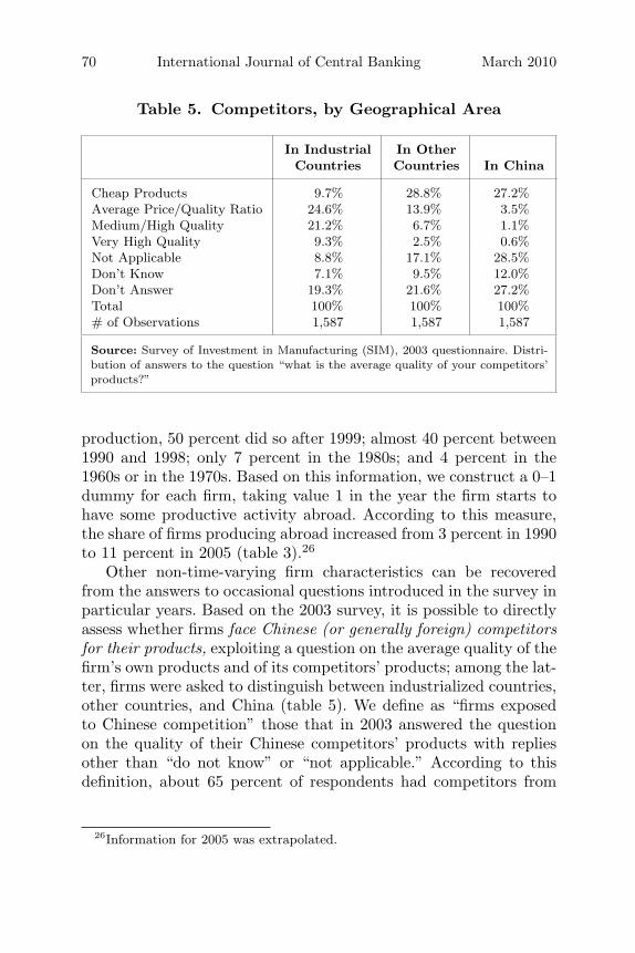
Other non-time-varying firm characteristics can be recoveredfrom the answers to occasional questions introduced in the survey inparticular years. Based on the 2003 survey, it is possible to directlyassess whether firms face Chinese (or generally foreign) competitorsfor their products, exploiting a question on the average quality of thefirm’s own products and of its competitors’ products; among the lat-ter, firms were asked to distinguish between industrialized countries,other countries, and China (table 5). We define as “firms exposedto Chinese competition” those that in 2003 answered the questionon the quality of their Chinese competitors’ products with repliesother than “do not know” or “not applicable.” According to thisdefinition, about 65 percent of respondents had competitors from

26Information for 2005 was extrapolated.


industrialized countries, while around 30 percent had competitorsfrom China in that year.

Among the remaining variables entering equation (7), nationalcontractual wages and the input deflator in manufacturing are fromIstat.27 The firm-specific ratio of labor costs over variable costs (λi)is taken from Gaiotti and Secchi (2006); it is constructed by merg-ing the SIM with the Central Accounts Data Service (firms’ balancesheets), taking the average share over the sample period for eachfirm.

4. Main Findings

4.1 Benchmark Specification

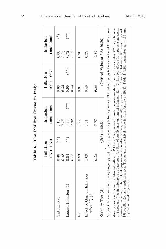
Table 6 shows that the flattening of the Phillips curve observed inthe main industrial countries is confirmed for Italy. The table reportsthe results of a regression of quarterly inflation on the output gap(measured as the deviation of GDP at constant prices from its HP-filtered trend) and its own lags. The effect of a change in the outputgap on inflation has constantly decreased since the 1970s. As shownin the last row of the table, in 1998–2006 a 1 percent increase in theoutput gap caused inflation to increase by slightly more than 0.2percentage points after three quarters; the same effect was almostdouble this large in the previous decade, and almost six times largerin the 1970s. The table also reports the results of a break-point test,which clearly rejects the hypothesis of coefficient stability.28

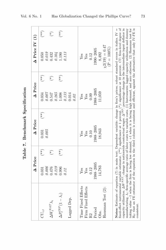
The estimates of equation (7) are reported in the first column oftable 7. Two conclusions stand out. The estimate of a1 is positive,around 0.03, and statistically significant. The size of the effect isalso plausible; the magnitude of the coefficient is comparable withthe macro estimates, once the different metrics of capacity utilization

27The intermediate input deflator is the ratio of the difference between produc-tion and value added at 1995 prices and the difference between production andvalue added at current prices.

28The table reports a sup-Chow statistic (the highest statistics from a sequenceof Chow tests with varying break dates) and the asymptotic critical value reportedby Andrews (1993). The estimation covers the last two decades for a comparisonwith the sample period of our micro data sample.


Tab

le6.

The

Phillips

Curv

ein

Ital

y

Inflat

ion

Inflat

ion

Inflat

ion

Inflat

ion

1970

–197

919

80–1

989

1990

–199

719

98–2

006

Out

put

Gap

0.46

(**)

0.18

0.09

0.08

(*)

0.18

0.15

0.06

0.04

Lag

ged

Infla

tion

(1)

0.94

(**)

0.96

(**)

0.90

(**)

0.72

(**)

0.05

0.02

0.06

0.09

R2

0.93

0.98

0.94

0.90

Effe

ctof

Gap

onIn

flati

onA

fter

3Q(2

)1.

690.

610.

400.

29

0.52

0.52

0.30

0.12

Stab

ility

Tes

t(3

)χ2(

6)=

80.5

4(C

riti

calV

alue

at5%

:20

.26)

Note

s:O

LS

esti

mat

eof

πt

=b 0

+b 1

ygap

t−1+

4 ∑ i=1c i

πt−

i,w

here

πtis

four

-qua

rter

CP

Iin

flati

on;y

gap t

isth

ede

viat

ion

ofG

DP

atco

n-

stan

tpr

ices

from

its

tren

d(o

btai

ned

wit

han

HP

filte

r);t

isqu

arte

rs.S

tand

ard

erro

rsar

esh

own

bel

owth

ees

tim

ates

.(**

):si

gnifi

canc

eat

1per

cent

;(*

):si

gnifi

canc

eat

10per

cent

.(1

)Su

mof

coeffi

cien

tson

lagg

edin

flati

on,Σ

c i.(2

)Im

plie

deff

ect

ofa

1-per

cent

age-

poi

ntper

sist

ent

incr

ease

inth

eou

tput

gap

onin

flati

onaf

ter

thre

equ

arte

rs.

(3)

Sequ

enti

alSu

p-C

how

χ2

stat

isti

cs.

Est

imat

ion

per

iod:

1986

–200

6.R

obus

tst

anda

rder

rors

.T

heas

ympt

otic

crit

ical

valu

eis

from

And

rew

s(1

993)

,Tab

le1

(wit

hpa

ram

eter

π0

=.1

5an

dde

gree

sof

free

dom

p=

6).


Tab

le7.

Ben

chm

ark

Spec

ifica

tion

ΔP

rice

ΔP

rice

ΔP

rice

ΔP

rice

IV(1

)

CU

i,t

0.03

1(*

*)0.

031

(**)

0.03

4(*

*)0.

050

(**)

0.00

60.

005

0.00

70.

019

ΔW

NAT

tλ

i0.

476

(*)

0.54

7(*

)0.

432

(*)

0.21

90.

265

0.30

4Δ

PIN

Pt

(1−

λi)

0.99

6(*

*)1.

098

(**)

1.19

0(*

*)0.

120.

133

0.11

3Lag

ged

Dep

.0.

014

0.02

Tim

eFix

edE

ffect

sY

esY

esY

esY

esFir

mFix

edE

ffect

sY

esY

esY

esY

esR

20.

120.

100.

090.

12Per

iod

1988

–200

519

88–2

005

1988

–200

519

90–2

005

Obs

.14

,783

18,9

4311

,059

8,49

2H

ausm

anTes

t(2

):χ2(

19)

=0.

47(P

=10

0%)

Note

s:E

stim

ate

ofeq

uati

on(7

)in

mai

nte

xt.

Dep

ende

ntva

riab

le:

chan

gein

firm

’spr

ices

;ro

bust

stan

dard

erro

rsin

ital

ics.

IV=

fixed

-effec

tin

stru

men

tal

vari

able

esti

mat

or.

(**)

:si

gnifi

canc

eat

1per

cent

.(*

):si

gnifi

canc

eat

10per

cent

.C

U:

firm

-lev

elde

gree

ofca

paci

tyut

iliza

tion

.Δ

WN

AT

:ch

ange

inna

tion

wid

eco

ntra

ctua

lw

ages

.Δ

INP

:per

cent

age

chan

gein

the

inte

rmed

iate

inpu

tde

flato

rin

man

ufac

turi

ng.λ

i:fir

m-s

pec

ific

aver

age

rati

oof

labor

cost

sto

vari

able

cost

s.(1

)In

stru

men

ts:la

gged

capa

city

utili

zati

onan

ddu

mm

yta

king

valu

e−

1w

hen

the

firm

isfa

cing

low

dem

and,

+1

whe

nit

isfa

cing

high

dem

and,

and

zero

othe

rwis

e.(2

)H

ausm

ante

stfo

rH

0:th

atan

FE

esti

mat

orof

the

equa

tion

inth

eth

ird

colu

mn

isco

nsis

tent

and

effici

ent,

agai

nst

the

alte

rnat

ive

that

only

IV-F

Eis

cons

iste

nt.


and the output gap has been taken into account.29 The estimates ofcoefficients b1 and b2, on the change in national contractual wagesand on the change in intermediate input costs (each multiplied bythe respective average share), are statistically significant, have theexpected sign, and are of the expected magnitude.30

The remaining columns present robustness checks. In the secondcolumn, the controls for input costs are dropped; the estimates of a1are unaffected. The third column presents the results of estimateswhich also include the lagged dependent on the right-hand side: theestimated coefficient on Δpi,t−1 is negligible (0.01) and not statis-tically different from zero.31 Finally, in the fourth column, instru-mental variables (IV) are used to address the potential endogeneityof CUi,t. The instruments used are the variables’ lagged values anda qualitative proxy for firm-specific shocks to demand, constructedfrom a question included in the SIM.32 A Hausman test overwhelm-ingly fails to reject the null hypothesis that the FE estimator isconsistent and efficient.

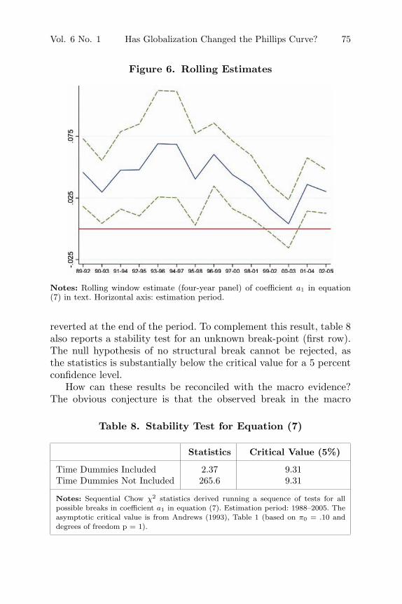
To investigate the existence of a break, in figure 6, we reportrolling estimates of a1, performed by running a series of regressionson panels covering a four-year span, starting with the period 1989–92 and then moving the window forward. The results are showntogether with 95 percent confidence bands. While the estimated coef-ficients somehow decrease over time, they mostly remain within theprevious periods’ confidence bands. Moreover, the decrease is fully

29A change in the output gap of 1 percentage point corresponds to a change inthe sample mean capacity utilization in SIM of about 2.5–3.0 percentage points.Hence, our estimate of a1 corresponds to an effect of the output gap on prices ofabout 0.08–0.09 within a year.

30The coefficient on contractual wages is lower than 1 (about 0.6), but this isa common finding (Gaiotti and Secchi 2006).

31The fixed-effects (FE) estimator may result in downward-biased estimates ofthe autoregressive coefficient; however, its use is appropriate when the numberof time periods is reasonably large, as in our sample. Alternative experimentsrun with a GMM first-difference estimator, not reported, still yielded resultsnot significantly different from those in the table (while implying the loss of aconsiderable number of observations).

32A dummy, taking value 1 in the case of an increase in demand, −1 in thecase of a decrease in demand, and zero otherwise, is based on two pieces ofinformation: whether the firm judges that the deviation between actual and pre-viously planned investment was due to unexpected demand behavior, and thequantitative difference between actual and planned investment.


Figure 6. Rolling Estimates

Notes: Rolling window estimate (four-year panel) of coefficient a1 in equation(7) in text. Horizontal axis: estimation period.

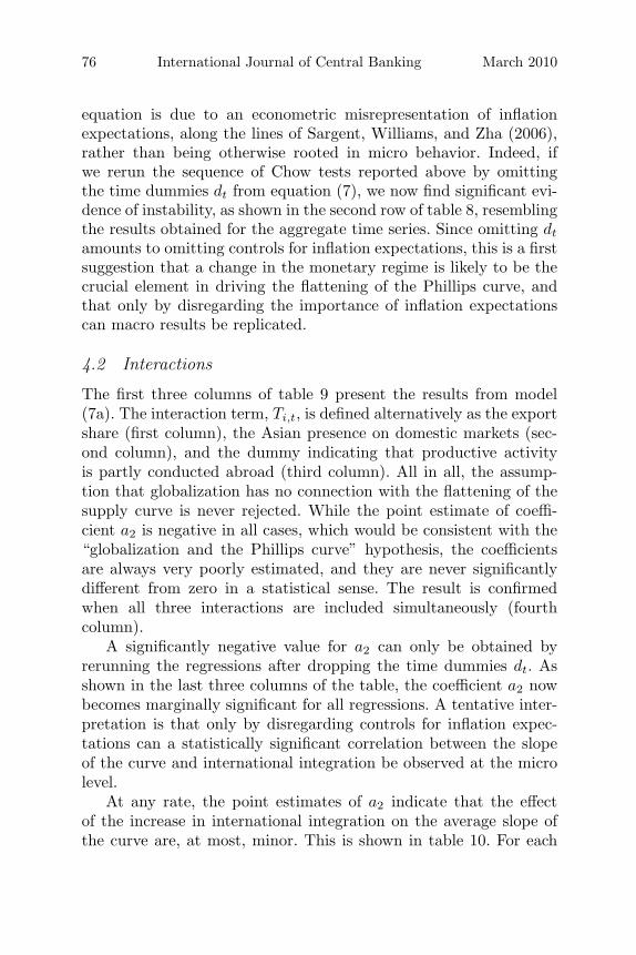
reverted at the end of the period. To complement this result, table 8also reports a stability test for an unknown break-point (first row).The null hypothesis of no structural break cannot be rejected, asthe statistics is substantially below the critical value for a 5 percentconfidence level.

How can these results be reconciled with the macro evidence?The obvious conjecture is that the observed break in the macro

Table 8. Stability Test for Equation (7)

Statistics Critical Value (5%)

Time Dummies Included 2.37 9.31Time Dummies Not Included 265.6 9.31

Notes: Sequential Chow χ2 statistics derived running a sequence of tests for allpossible breaks in coefficient a1 in equation (7). Estimation period: 1988–2005. Theasymptotic critical value is from Andrews (1993), Table 1 (based on π0 = .10 anddegrees of freedom p = 1).


equation is due to an econometric misrepresentation of inflationexpectations, along the lines of Sargent, Williams, and Zha (2006),rather than being otherwise rooted in micro behavior. Indeed, ifwe rerun the sequence of Chow tests reported above by omittingthe time dummies dt from equation (7), we now find significant evi-dence of instability, as shown in the second row of table 8, resemblingthe results obtained for the aggregate time series. Since omitting dt

amounts to omitting controls for inflation expectations, this is a firstsuggestion that a change in the monetary regime is likely to be thecrucial element in driving the flattening of the Phillips curve, andthat only by disregarding the importance of inflation expectationscan macro results be replicated.

4.2 Interactions

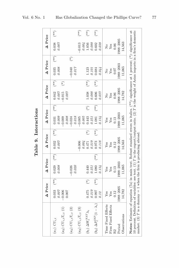
The first three columns of table 9 present the results from model(7a). The interaction term, Ti,t, is defined alternatively as the exportshare (first column), the Asian presence on domestic markets (sec-ond column), and the dummy indicating that productive activityis partly conducted abroad (third column). All in all, the assump-tion that globalization has no connection with the flattening of thesupply curve is never rejected. While the point estimate of coeffi-cient a2 is negative in all cases, which would be consistent with the“globalization and the Phillips curve” hypothesis, the coefficientsare always very poorly estimated, and they are never significantlydifferent from zero in a statistical sense. The result is confirmedwhen all three interactions are included simultaneously (fourthcolumn).

A significantly negative value for a2 can only be obtained byrerunning the regressions after dropping the time dummies dt. Asshown in the last three columns of the table, the coefficient a2 nowbecomes marginally significant for all regressions. A tentative inter-pretation is that only by disregarding controls for inflation expec-tations can a statistically significant correlation between the slopeof the curve and international integration be observed at the microlevel.

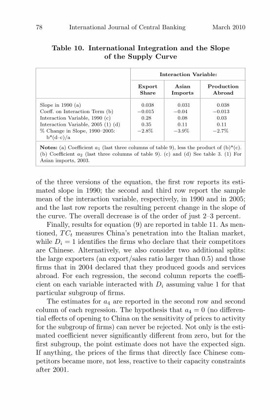
At any rate, the point estimates of a2 indicate that the effectof the increase in international integration on the average slope ofthe curve are, at most, minor. This is shown in table 10. For each


Tab

le9.

Inte

ract

ions

ΔP

rice

ΔP

rice

ΔP

rice

ΔP

rice

ΔP

rice

ΔP

rice

ΔP

rice

(a1)

CU

i,t

0.03

3(*

*)0.

029

(**)

0.03

2(*

*)0.

031

(**)

0.04

2(*

*)0.

035

(**)

0.03

8(*

*)0.

007

0.00

80.

007

0.00

90.

007

0.00

80.

007

(a2)

CU

i,tT

i,t

(1)

−0.

006

−0.

009

−0.

015

(*)

0.00

70.

008

0.00

7(a

2)

CU

i,tT

i,t

(2)

−0.

026

−0.

024

−0.

040

(*)

0.02

00.

018

0.01

7(a

2)

CU

i,tT

i,t

(3)

−0.

006

−0.

005

−0.

013

(**)

0.00

40.

005

0.00

4(b

1)

ΔW

NAT

tλ

i0.

475

(*)

0.44

00.

471

(*)

0.44

3(*

)1.

038

(**)

1.12

31.

056

(**)

0.21

90.

251

0.21

90.

251

0.08

80.

101

0.08

8(b

2)

ΔP

INP

t(1

−λ

i)

0.99

7(*

*)1.

080

(**)

0.97

3(*

*)1.

081

(**)

0.60

6(*

*)0.

684

0.60

2(*

*)0.

120.

134

0.11

80.

134

0.03

70.

044

0.03

8

Tim

eFix

edE

ffec

tsY

esY

esY

esY

esN

oN

oN

oFir

mFix

edE

ffec

tsY

esY

esY

esY

esY

esY

esY

esR

20.

120.

130.

120.

130.

060.

070.

06Per

iod

1988

–200

519

88–2

003

1988

–200

519

88–2

003

1988

–200

519

88–2

003

1988

–200

5O

bser

vati

ons

14,7

8211

,065

14,5

6311

,065

14,7

8211

,065

14,5

63

Note

s:E

stim

ate

ofeq

uati

on(7

a)in

mai

nte

xt.R

obus

tst

anda

rder

rors

init

alic

s.(*

*):si

gnifi

canc

eat

1per

cent

;(*

):si

gnifi

canc

eat

10per

cent

.D

efini

tion

ofva

riab

les:

see

text

.(1

)T

isth

eex

por

t/ou

tput

rati

o.(2

)T

isth

ew

eigh

tof

Asi

anim

por

tsin

afir

m’s

dom

esti

cm

arke

t.(3

)T

isa

dum

my

=1

whe

nth

efir

mis

prod

ucin

gab

road

.


Table 10. International Integration and the Slopeof the Supply Curve

Interaction Variable:

Export Asian ProductionShare Imports Abroad

Slope in 1990 (a) 0.038 0.031 0.038Coeff. on Interaction Term (b) −0.015 −0.04 −0.013Interaction Variable, 1990 (c) 0.28 0.08 0.03Interaction Variable, 2005 (1) (d) 0.35 0.11 0.11% Change in Slope, 1990–2005:

b*(d–c)/a−2.8% −3.9% −2.7%

Notes: (a) Coefficient a1 (last three columns of table 9), less the product of (b)*(c).(b) Coefficient a2 (last three columns of table 9). (c) and (d) See table 3. (1) ForAsian imports, 2003.

of the three versions of the equation, the first row reports its esti-mated slope in 1990; the second and third row report the samplemean of the interaction variable, respectively, in 1990 and in 2005;and the last row reports the resulting percent change in the slope ofthe curve. The overall decrease is of the order of just 2–3 percent.

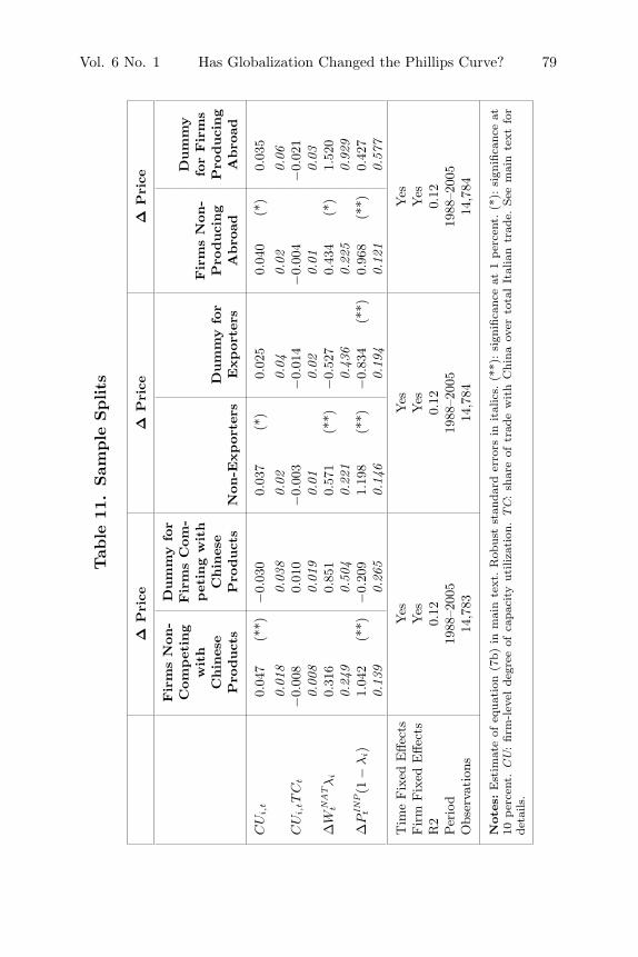
Finally, results for equation (9) are reported in table 11. As men-tioned, TCt measures China’s penetration into the Italian market,while Di = 1 identifies the firms who declare that their competitorsare Chinese. Alternatively, we also consider two additional splits:the large exporters (an export/sales ratio larger than 0.5) and thosefirms that in 2004 declared that they produced goods and servicesabroad. For each regression, the second column reports the coeffi-cient on each variable interacted with Di assuming value 1 for thatparticular subgroup of firms.

The estimates for a4 are reported in the second row and secondcolumn of each regression. The hypothesis that a4 = 0 (no differen-tial effects of opening to China on the sensitivity of prices to activityfor the subgroup of firms) can never be rejected. Not only is the esti-mated coefficient never significantly different from zero, but for thefirst subgroup, the point estimate does not have the expected sign.If anything, the prices of the firms that directly face Chinese com-petitors became more, not less, reactive to their capacity constraintsafter 2001.


Tab

le11

.Sam

ple

Splits

ΔP

rice

ΔP

rice

ΔP

rice

Fir

ms

Non

-D

um

my

for

Com

pet

ing

Fir

ms

Com

-D

um

my

wit

hpet

ing

wit

hFir

ms

Non

-fo

rFir

ms

Chin

ese

Chin

ese

Dum

my

for

Pro

duci

ng

Pro

duci

ng

Pro

duct

sP

roduct

sN

on-E

xpor

ters

Expor

ters

Abro

adA

bro

ad

CU

i,t

0.04

7(*

*)−

0.03

00.

037

(*)

0.02

50.

040

(*)

0.03

50.

018

0.03

80.

020.

040.

020.

06C

Ui,

tT

Ct

−0.

008

0.01

0−

0.00

3−

0.01

4−

0.00

4−

0.02

10.

008

0.01

90.

010.

020.

010.

03Δ

WN

AT

tλ

i0.

316

0.85

10.

571

(**)

−0.

527

0.43

4(*

)1.

520

0.24

90.

504

0.22

10.

436

0.22

50.

929

ΔP

INP

t(1

−λ

i)

1.04

2(*

*)−

0.20

91.

198

(**)

−0.

834

(**)

0.96

8(*

*)0.

427

0.13

90.

265

0.14

60.

194

0.12

10.

577

Tim

eFix

edE

ffect

sY

esY

esY

esFir

mFix

edE

ffect

sY

esY

esY

esR

20.

120.

120.

12Per

iod

1988

–200

519

88–2

005

1988

–200

5O

bser

vati

ons

14,7

8314

,784

14,7

84

Note

s:E

stim

ate

ofeq

uati

on(7

b)in

mai

nte

xt.R

obus

tst

anda

rder

rors

init

alic

s.(*

*):si

gnifi

canc

eat

1per

cent

.(*

):si

gnifi

canc

eat

10per

cent

.C

U:

firm

-lev

elde

gree

ofca

paci

tyut

iliza

tion

.T

C:

shar

eof

trad

ew

ith

Chi

naov

erto

tal

Ital

ian

trad

e.Se

em

ain

text

for

deta

ils.


5. Conclusions

It has been conjectured that the flattening of the Phillips curveobserved at the macroeconomic level is a structural feature ofadvanced economies, and that it is a consequence of globalization.The most compelling arguments rely either on a change in the behav-ior of individual firms’ markups, which may have become morecountercyclical in order to defend market shares, or on a less upward-sloping curve for firm-specific inputs: companies that are delocalizingproduction may exploit a pool of labor more elastically supplied,and their workers may make less aggressive demands for increasedovertime compensation when the level of activity rises.

We argued that a testable implication of this conjecture isthat a change in the sensitivity of prices to capacity utilization isapparent not only in macroeconomic time series but also at thefirm level, that this result is robust to controls for economy-wideinflation expectations, and that such a change has also been con-centrated among the firms that are most exposed to internationalcompetition.

Using the micro data from the Bank of Italy’s Survey of Invest-ment in Manufacturing, we are able to test whether these implica-tions are observable. The answer is either inconclusive or negative.A statistically significant flattening of the supply curve can only bereplicated at the micro level by running a (possibly misspecified)regression which omits controlling time fixed effects. The interac-tion coefficient with various measures of firms’ international integra-tion has the expected sign, but it is not significantly different fromzero and (more importantly) its point estimates indicate an eco-nomically irrelevant effect at the macro level. The effect of China’sentry on firms that are most exposed to that country’s competitionwas, if any, of the opposite sign to the one that could have beenexpected.

The results give no support to the conjecture that the flat-tening of the Phillips curve is rooted in the different behavior ofindividual firms exposed to competition. There seems to be littleempirical ground in our data to discard the traditional view thata more moderate dynamic of inflation expectations is by far themain force driving the observed changes in the slope of the curve. Inour view, the result suggests that institutional and policy changes


which occurred in the first half of the 1990s remain the most likelyexplanation of the macro findings. As far as the empirical evidencecurrently stands, monetary policymakers would be ill advised toreconsider their “beliefs” and their strategies.

While we find no support for the conjecture that globalizationaffected the Phillips curve, our results do not imply that it had noeffect on firms’ pricing. Our results are not inconsistent with theargument that trade is likely to have acted as a favorable directshock on the prices of the firms that were most exposed to inter-national competition, possibly with substantial benefits for the con-sumers. A thorough assessment of this issue is beyond the scope ofthis paper, although various pieces of empirical analysis for OECDcountries, mentioned in the paper, seem to be consistent with thisconjecture.

References

Altig, D., L. Christiano, M. Eichenbaum, and J. Linde. 2005. “Firm-Specific Capital, Nominal Rigidities and the Business Cycle.”NBER Working Paper No. 11034.

Altissimo, F., E. Gaiotti, and A. Locarno. 2001. “Monetary Analysisin the Bank of Italy Prior to EMU.” In Monetary Analysis: Toolsand Applications, ed. H. J. Klockers and C. Willeke, 145–64.Frankfurt am Main: European Central Bank.

Andrews, D. W. K. 1993. “Tests for Parameter Instability and Struc-tural Change with Unknown Change Point.” Econometrica 61(4): 821–56.

Ball, L. M. 2006. “Has Globalization Changed Inflation?” NBERWorking Paper No. 12687.

Ball, L. M., N. G. Mankiw, and D. Romer. 1988. “The New Keyne-sian Economics and the Output-Inflation Trade-off.” BrookingsPapers on Economic Activity 1: 1–82.

Ball, L., and D. Romer. 1990. “Real Rigidities and the Non-neutrality of Money.” Review of Economic Studies 57 (2): 183–203.

Banca d’Italia. 2005. “Italian Foreign Trade in Textiles and Cloth-ing After Liberalization.” Economic Bulletin 41 (November):26–27.


———. 2006. “La bilancia dei pagamenti e la posizione nettasull’estero.” Relazione del Governatore sull’anno 2005.

Bank for International Settlements. 2006. “Globalisation and Mon-etary Policy.” In 76thAnnual Report, 69–78. Basel, Switzerland:Bank for International Settlements.

Bean, C. 2006a. “Commentary: Impact of Globalization on Mone-tary Policy.” Comments on a paper by Ken Rogoff. See Rogoff(2006).

Bean, C. 2006b. “Globalisation and Inflation.” Quarterly Bulletin(Bank of England) 46 (4): 468–75.

Borio, C. E. V., and A. Filardo. 2007. “Globalisation and Infla-tion: New Cross-Country Evidence on the Global Determinantsof Domestic Inflation.” BIS Working Paper No. 227.

Brandolini, A., P. Casadio, P. Cipollone, M. Magnani, A. Rosolia,and R. Torrini. 2007. “Employment Growth in Italy in the 1990s:Institutional Arrangements and Market Forces.” In Social Pacts,Employment and Growth, ed. N. Acocella and R. Leoni, 31–68.Heidelberg: Physica-Verlag.

Bugamelli, M. 2007. “Export Prices, Product Quality and Firms’Characteristics: An Analysis on a Sample of Italian Firms.”Banca d’Italia Temi di discussione No. 634.

Bugamelli, M., S. Fabiani, and E. Sette. 2009. “The Pro-competitiveEffect of Imports from China: An Analysis on Firm-Level PriceData.” (September).

Chen, N., J. Imbs, and A. Scott. 2004. “Competition, Globaliza-tion and the Decline of Inflation.” CEPR Discussion PaperNo. 4695.

Daniels, J. P., F. Nourzad, and D. D. Vanhoose. 2005. “Openness,Central Bank Independence and the Sacrifice Ratio.” Journal ofMoney, Credit, and Banking 37 (2): 371–79.

European Central Bank. 2005. “Competitiveness and the ExportPerformance of the Euro Area.” Report by a Task Force ofthe Monetary Policy Committee of the ESCB, ECB OccasionalPaper No. 30.

Fabiani, S., A. Gattulli, and R. Sabbatini. 2007. “The Pricing Behav-ior of Italian Firms: New Survey Evidence on Price Stickiness.”In Pricing Decisions in the Euro Area: How Firms Set Pricesand Why, ed. S. Fabiani, C. S. Loupias, F. M. Martins, andR. Sabbatini. Oxford University Press.


Fabiani, S., A. Gattulli, R. Sabbatini, and G. Veronese. 2006. “Con-sumer Price Setting in Italy.” Giornale degli Economisti e Annalidi Economia 65 (1): 31–74.

Gaiotti, E. 2008. “Has Globalization Changed the Phillips Curve?Firm-Level Evidence on the Effect of Activity on Prices.” Bancad’Italia, Temi di discussione No. 676.

Gaiotti, E., and A. Secchi. 2006. “Is There a Cost Channel ofMonetary Policy Transmission? An Investigation into the Pric-ing Behaviour of 2,000 Firms.” Journal of Money, Credit, andBanking 38 (8): 2013–37.

Ihrig, J., S. B. Kamin, D. Lindner, and J. Marquez. 2007. “Some Sim-ple Tests of the Globalization and Inflation Hypothesis.” Inter-national Finance Discussion Paper No. 891, Board of Governorsof the Federal Reserve System.

International Monetary Fund. 2006. “How Has GlobalizationAffected Inflation?” In World Economic Outlook (April). Wash-ington, DC: International Monetary Fund.

Kamin, S. B., M. Marazzi, and J. W. Schindler. 2004. “Is China‘Exporting Deflation’?” International Finance Discussion PaperNo. 791, Board of Governors of the Federal Reserve System.

Kohn, D. L. 2006. “The Effects of Globalization on Inflation andTheir Implications for Monetary Policy.” Speech at the FederalReserve Bank of Boston 51st Economic Conference, Chatham,Massachusetts, June 16.

Pain, N., I. Koske, and M. Sollie. 2006. “Globalisation and Infla-tion in the OECD Economies.” OECD Economics Department,Working Paper No. 524.

Razin, A., and P. Loungani. 2005. “Globalization and Inflation-Output Tradeoffs.” NBER Working Paper No. 11641.

Rogoff, K. 2006. “The Impact of Globalisation on Monetary Pol-icy.” Presented at the Federal Reserve Bank of Kansas City 30th

Annual Economic Symposium, Jackson Hole, Wyoming, August24–26.

Romer, D. 1993. “Openness and Inflation: Theory and Evidence.”Quarterly Journal of Economics 108 (4): 869–904.

Rotemberg, J. J., and M. Woodford. 1999. “The Cyclical Behaviorof Prices and Costs.” In The Handbook of Macroeconomics, Vol.1A, ed. J. Taylor and M. Woodford. North-Holland.


Sargent, T. J., N. Williams, and T. Zha. 2006. “Shocks and Govern-ment Beliefs: The Rise and Fall of American Inflation.” AmericanEconomic Review 96 (4): 1193–24.

Temple, J. 2002. “Openness, Inflation and the Phillips Curve: APuzzle.” Journal of Money, Credit, and Banking 34 (2): 450–68.

Woodford, M. 2007. “Globalization and Monetary Control.” NBERWorking Paper No. 13329.

Has Globalization Changed the Phillips Curve? Firm … · Has Globalization Changed the Phillips...

Documents

Transcript of Has Globalization Changed the Phillips Curve? Firm … · Has Globalization Changed the Phillips...