Harvest Forecasting with Environmental Information for ... · Harvest Forecasting with...

Journal of Advanced Agricultural Technologies Vol. 2, No. 2, December 2015

83© 2015 Journal of Advanced Agricultural Technologiesdoi: 10.12720/joaat.2.2.83-87

Harvest Forecasting with Environmental

Information for Cucumbers Cultivated in Net

Houses

Yung-Hsing Peng, Chin-Shun Hsu, and Po-Chuang HuangInnovative DigiTech-Enabled Applications and Services Institute, Institute for Information Industry

Kaohsiung City, 80661 Taiwan

Email: {pengyh, ling9082, arvinpchuang}@iii.org.tw

Abstract—For the purpose of supply chain management, a

crop producer is required to forecast and to forward the

information of potential harvest to his customers, such as

food processors or wholesale channels. Usually, such

forecast relies on the field observation done by experienced

producers with domain knowledge for growing crops under

different climates. In this paper, we propose a

computational approach for cucumber harvest forecasting,

which is based on the partial least square (PLS) regression

over historical environment and harvest information. The

experiment is performed in a 40×8m2 net house consisting

36 tiny farms for collecting the harvest data, and 68

environmental sensors for measuring the illumination, the

air temperature, the air humidity, the soil temperature, and

the soil moisture. The area of each tiny farm is about 8m2,

which is planted with 16 seedlings of organic cucumbers.

The harvest and the environmental data are collected with

the Smart Agro-management Platform (SAMP) developed

by the Institute for Information Industry (III). According to

the experimental results, the forecast for the accumulative

harvest in the future 4 to 6 days achieves accuracy 70% in

split testing, which is close to the averaged forecasting

performance of experienced producers. Therefore, the

environmental data during the harvest season serves as

good factors for building harvest forecasting models.

Index Terms—cucumber, data science, environmental

factors, harvest forecasting

I. INTRODUCTION

Harvest forecasting is an important application of data

science to modern agriculture, which helps to determine

whether the supply meets the demand. In addition, by

integrating forecasting models for individual lands, crop

production scheduling can be more systematic to

managers and more applicable to future sales. To

construct a harvest forecasting model, factors related to

harvest have to be defined, collected, and analyzed during

the progress. For example, Aggelopoulou et al. [1]

predicts the yield of apples by taking the density of apple

flowers as the factor, which is obtained from image

processing. As another example, Yang et al. [2] estimates

the crop yield by analyzing the hyperspectral images

collected from airplanes or satellites. In addition to

Manuscript received March 17, 2015; revised May 4, 2015.

images and spectral signals, environmental information is

supposed to be of high relevance to crop growth and

harvest, and therefore many researchers focus on finding

the relationship between environment and harvest [3]-[5],

in order to improve the accuracy of harvest forecasting.

In general, such relationship can be expressed by linear or

non-linear model. For building linear model, the partial

least square (PLS) regression [6] is an effective and well-

known technique, which has been widely applied in

previous works. Meanwhile, the multi-degree polynomial

model [7]-[9] and the artificial neural network [10], [11]

are usually adopted for non-linear analysis.

To increase the harvest, plenty of crops in Taiwan are

now cultivated in nethouses (simplified greenhouses with

few facilities). Among these crops, cucumber is a very

popular vegetable for Taiwanese, which usually comes in

the form of side dishes. If cultivated in net houses, the

growing season of cucumber takes about 45 to 60 days,

which is followed by the flowering season of 5 to 7 days.

After that, the cucumber can be harvested for 2 to 4

weeks, depending on the cultivation managment. To our

knowledge, the interaction between fertilizers and

cucumber growth behaviors have been extensively

studied in previous researches [12]-[15]. However, most

of these researches focus on evaluating the effectiveness

of certain fertilizer, rather than forecasting the harvest in

the future. In the field of agricultural data science,

computational approach that forecasts the harvest of

cucumber is scarcely investigated, which remains worthy

of study. In this paper, we propose a harvest forecasting

approach that takes the environmental data in the past as

factors, and forecasts the acumulative harvest in a future

period of time. The required data are collected with the

Smart Agro-management Platform (SAMP), an

agricultural cloud service developed by the Institute for

Information Industry (III). The organization of this paper

is as follows. In Section II, we present the main

architecture and concise descriptions for our

computational model. After that, the experimental results

are given in Section III. Finally, we give our conclusions

and some future studies in Section IV.

II. METHODOLOGY

The flowchart for building our forecasting model is

shown in Fig. 1, consisting of six main steps (1) the raw


84© 2015 Journal of Advanced Agricultural Technologies

data acquisition, (2) the sensor data preprocessing, (3) the

tiny climate allocation, (4) the dataset creation, (5) the

model construction, and (6) the verification. In Fig. 1, the

items with yellow background represent the techniques

involved in each step, explained as follows.

Figure 1. The flowchart for building the harvest forecasting model.

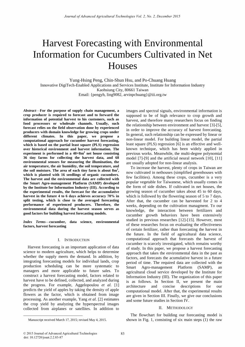
Figure 2. The layout of 68 sensors and 36 tiny farms in the experimental net house.

A. Raw Data Acquisition

There are two kinds of raw data adopted in this paper,

which are the environmental data obtained by sensors,

and the harvest data reported by farmers. To store the

obtained data, we utilize the Smart Agro-management

Platform (SAMP) developed by the Institute for

Information Industry (III), which offers convenient

service for agricultural management. The SAMP gathers

environmental data from the gateway of III, which is a

box with network access, connected by many sensors and

placed in the cucumber net house. At the same time, the

fulfillment of farming task is reported to SAMP by a

farming app, by which farmers can take pictures and

input the daily yield during the harvest season. The yield

data is directly sent to the database of SAMP, whereas the

environmental data is preprocessed by the gateway before

transmission to SAMP.

B. Sensor Data Preprocessing

In our research, 68 sensors with 1-minute sampling

rate are placed in the experimental net house, and the

gateway reports the processed data of each sensor for

every 10 minutes, removing the outliers that do not fall

within 2 standard deviations to the average. For the

purpose of analysis, the reported data to SAMP is

furthered averaged to obtain the hourly records of

environment, which serves as our environmental factors

for harvest forecasting.

C. Tiny Climate Allocation

To obtain suitable amount of harvest data, the net

house is divided into tiny farms. By referring to the

layout of sensors and tiny farms (such as Fig. 2), the

climate of each tiny farm is estimated with the inverse

distance weighting technique [16]. For a specified type of

environment k, such as the air temperature, the climate

Ck(u) of the tiny farm u is estimated by the formula

𝐶𝑘(𝑢) =∑ 𝐼(𝑢,𝑣𝑘,𝑗)×𝑣𝑎𝑙(𝑣𝑘,𝑗)𝑗

∑ 𝐼(𝑢,𝑣𝑘,𝑗)𝑗 (1)

where I(u, vk,j) denotes the inverse distance weight for the

tiny farm u and the jth sensor for measuring environment

k in the net house, and val(vk,j) is the sensing value of

sensor vk,j. Usually, I(u, vk,j) is computed as 1/D(u, vk,j)p,

where D(u, vk,j) represents the distance between the center

of u and the location of vk,j, which can be estimated by the

Euclidean distance or the Hamming distance. In addition,

the variable p is used to control the inverse weight. In this

paper, the considered environments are the illumination

for k=1, the air temperature for k=2, the air humidity for

k=3, the soil temperature for k=4, and the soil moisture

for k=5. Note that the numbers of sensors placed for each

36 tiny farms

4 wooden stands in

each tiny farm, with 16

cucumber seedlings.

Air Temperature

Air Humidity

Illumination

Soil Temperature

Soil Moisture

Illumination

Soil Temperature

Soil Moisture

Soil Temperature

Soil Moisture

40 m

8 m

F1 F2 F3

F10

F19

F28

Door

0

2

4

6

8

5 10 15 20 25 30 35 40



environment could be different. Because the

environmental data is hourly recorded in the SAMP

database, we can obtain 524=120 environmental records

for each tiny farm per day.

D. Dataset Creation

The environmental and harvest records are further

integrated to create our dataset. For investigating the

continuous effect of environment to harvest, we construct

our datasets according to the harvest date t with two

variables r1 and r2. In each dataset, the environments

obtained from dates (t – r1) to (t – 1) are taken as the

factors, and the forecasting target is the accumulative

harvest from dates t to (t + r2 – 1). By accumulating the

harvest, the noise caused by holiday (zero harvest) can be

reduced. For specified r1 and r2, the data is of dimension

(r1×120 + 1). By manipulating r1 and r2, individual

datasets can be generated for experiment, which will be

further explained in Section III. The generated datasets

are stored as .arff files, which can be accessed by the

Weka software [17] for model construction.

E. Model Construction

For each created dataset, we perform the partial least

square (PLS) regression [6] to construct the forecasting

model. Here we merely give a brief explanation to the

PLS regression, but omit the detailed computation,

because it is beyond the scope of this paper. Let X be an n

× m matrix that keeps n records of environments, where

m = r1× 120, and let Y be an n × 1 matrix that keeps n

records of accumulative yield. The PLS regression

detects the relationship between X and Y by the following

decomposition

X = TPT + E

Y = UQT + F (2)

where T and U are n × s matrices, P is an m × s matrix, Q

is a 1 × s matrix, E is an n × m matrix, and F is an n × 1

matrix. The purpose of this decomposition is to find the

matrices T and U of the highest relevance for building the

linear regression U=TB, where B is the coefficient matrix

of size s × s. With the above decomsition, the yield

forecasting Ynew to a given environment record Xnew of

size 1 × m can be accomplished as follows.

Step 1: Compute the 1s matrix Tnew=XnewP

Step 2: Compute the 1s matrix Unew = TnewB

Step 3: Compute the 11 matrix Ynew = UnewQT

For ease of implementation, the Weka software [17] is

adopted for the computation of PLS, which also offers

convenient tools for viewing data statistics and verifying

model performance.

F. Verification

The verification of models is accomplished with the

self-testing and split-testing functions in Weka. We

estimate the accuracy of a model by (1)the mean absolute

error (MAE) of the overall forecasting and (2)the mean

accumulative harvest of the dataset. Formally, the

accuracy for the model with r1 = i and r2 = j is defined as

acci,j = 1 – (Ri,j / Hj) (3)

where Ri,j and Hi,j are the MAE of the model and the

mean accumulative harvest for j days, respectively. In

addition, the ratio term Ri,j / Hj represents the degree of

error. The description of our methodolgy ends here, and

in the following we propose our experimental results.

III. EXPERIMENTS

To cultivate cucumbers, we rented a 40×8m2 net house

in the Yongling Organic Farm located in Kaohsiung. The

cultivation tasks were managed by an agricultural expert

in the Kaohsiung District Agricultural Research and

Extension Station, and these tasks were fulfilled by

farmers in Yongling. The cucumber seedlings were

planted on March 1st in 2014, and the harvest season was

from April 6th

to May 9th

in 2014. To obtain appropriate

amount of data, the net house was furthered divided into

36 tiny farms of area 8m2 for reporting the harvest, and

the environmental data was collected with 68 sensors.

There were 16 planted cucumber seedlings in each tiny

farm. During our experiment, the SAMP received the

environmental reports in every 10 minutes (which is

further organized to hourly records), and received the

cultivation reports from the farmers everyday. The layout

of 68 sensors and 36 tiny farms are shown in Fig. 2, in

which the entrance (door) of net house is placed on the

left. Note that sensors for different environements could

be placed on the same position. For example, the red

circles in Fig. 2 specify the locations containing five

sensors, and for yellow triangles we place two kinds of

sensors on them.

TABLE I. THE ACCURACIES OF 36 HARVEST FORECASTING MODELS FOR CUCUMBERS.

r2 = 1 r2 = 2 r2 = 3 r2 = 4 r2 = 5 r2 = 6

Train

(754)

Test

(260)

Train

(754)

Test

(220)

Train

(754)

Test

(219)

Train

(754)

Test

(183)

Train

(754)

Test

(145)

Train

(754)

Test

(109)

r1 = 1 55.81% 46.99% 62.42% 48.76% 69.66% 56.82% 73.40% 66.64% 75.94% 71.95% 76.85% 75.04%

r1 = 2 58.58% 50.31% 64.15% 52.04% 72.06% 59.24% 74.48% 70.76% 76.01% 70.60% 78.04% 73.95%

r1 = 3 60.65% 51.31% 67.89% 42.92% 73.30% 63.78% 75.53% 72.22% 77.34% 70.26% 79.26% 73.18%

r1 = 4 62.32% 52.24% 69.09% 52.29% 73.55% 64.44% 76.11% 64.56% 78.31% 63.05% 79.86% 69.80%

r1 = 5 62.42% 52.47% 68.99% 55.80% 73.64% 59.02% 76.64% 56.36% 78.60% 60.45% 79.81% 70.74%

r1 = 6 63.92% 48.06% 70.43% 57.80% 75.24% 51.93% 77.67% 59.36% 79.34% 60.38% 80.48% 68.48%

Hr2 (kg) 0.79 1 1.331 1.351 1.994 2.183 2.65 2.774 3.259 3.763 3.882 3.96



(a) self-testing for r1=3 and r2=4 (b) self-testing for r1=1 and r2=5 (c) self-testing for r1=1 and r2=6

(d) split-testing for r1=3 and r2=4 (e) split-testing for r1=1 and r2=5 (f) split-testing for r1=1 and r2=6

Figure 3. The distribution of forecast for self-testing and split testing.

For identification, the 36 tiny farms are named as F1,

F2, …, F36, and the centers (coordinates) for F1 to F9 are

(4, 1), (8, 1),…, (36, 1). Similarly, the centers for F10 to

F18, F19 to F27, and F28 to F36 locate at (4, 3) to (36, 3),

(4, 5) to (36, 5), and (4, 7) to (36, 7), respectively. These

coordinates are utilized to perform the tiny climate

allocation, as mentioned in Section II.C. In our

experiment, we investigate r1 and r2 from 1 to 6,

generating 36 datasets for building forecasting models.

The number of components c for executing Weka PLS is

set to 10. For split-testing, the data obtained before May

1st

serve as the training data, and the others are the testing

data. The accuracies of self-testing (Train) and split-

testing (Test) are given as Table I, where the numbers in

parentheses are sizes of datasets, and Hr2 provides the

mean accumulative harvest for r2 days in the dataset. The

accuracies in split-testing are marked with bold and blue

if they are higher than 70%. In addition, we further

investigate the distribution of forecast for the best models

obtained with r2=4, r2=5, and r2=6, whose accuracies for

split-testing are 72.22%, 71.95%, and 75.04%,

respectively. In Fig. 3, we provide diagrams for both the

self-testing and the split-testing. Interestingly, we find

that these forecasting models tend to give under-

estimation because there are only few forecasts greater

than 5kg. However, it is obvious that many real harvests

exceed 5kg.

Finally, the total yield of each tiny farm during the

harvest season April 6th

to May 9th

in 2014 is illustrated

as Fig. 4. The overall yield obtained from the net house is

850.62 kg, and the highest and lowest yields are produced

by F12 and F18, which are 32.34 kg and 12.48 kg,

respectively.

Figure 4. The total yield of 36 tiny farms.

IV. CONCLUSION

From Table I, one can see that the environmental

information of the past 2 or 3 days can be used to forecast

the accumulative harvest for the future 4 to 6 days,

achieving accuracies higher than 70%. According to our

interview with experienced farmers, the achieved

accuracies are close to that of their own forecasts, which

reveals the initial contribution of our computational

approach. For future study, we will devise non-linear and

evolutionary models to improve the forecasting accuracy.

Referring to our previous research, the response surface

methodology (RSM) [18] is worth being investigated to

achieve this goal. In addition, we would like to consider



the post-calibration mechanism, since our models reveal

the bias of under-estimation. We will also extend our

approach to support climate stations and real fields,

which are more general compared with sensors and tiny

farms. Finally, the frequencies and timing of farming

tasks are factors that have not yet been considered, which

could be included in the future research to analyze the

relationship between task schedule and harvest.

ACKNOWLEDGMENT

This study is conducted under the "Online and Offline

integrated Smart Commerce Platform (2/4)" of the

Institute for Information Industry which is subsidized by

the Ministry of Economy Affairs of the Republic of

China. The authors would like to express their

appreciation to the staff of Yongling Organic Farm and

Kaohsiung District Agricultural Research and Extension

Station for their kind support on cucumber production

management and harvest data collection.

REFERENCES

[1] D. Aggelopoulou, D. Bochtis, S. Fountas, K. C. Swain, T. A.

Gemtos, and G. D. Nanos, “Yield prediction in apple orchards

based on image processing,” Precision Agriculture, vol. 12, pp. 448-456, 2011.

[2] C. Yang, J. H. Everitt, Q. Du, B. Luo, and J. Chanussot, “Using

high-resolution airborne and satellite imagery to assess crop growth and yield variability for precision agriculture,”

Proceedings of the IEEE, vol. 101, no. 3, pp. 582-592, 2013.

[3] J. Arnó, J. R. Rosell, R. Blanco, M. C. Ramos, J. A. Martínez-Casasnovas, “Spatial variability in grape yield and quality

influenced by soil and crop nutrition characteristics,” Precision

Agriculture, vol. 13, pp. 393-410 , 2012. [4] W. S. Lee, V. Alchanatis, C. Yang, M. Hirafuji, D. Moshou, C. Li,

“Sensing technologies for precision specialty crop production,”

Computers and Electronics in Agriculture, vol. 74, pp. 2-33, 2010. [5] M. Ruiz-Altisent, L. Ruiz-Garcia, G. P. Moreda, et al., “Sensors

for product characterization and quality of specialty crops—A

review,” Computers and Electronics in Agriculture, vol. 74, pp. 176-194, 2010.

[6] R. Rosipal and N. Krämer, “Overview and recent advances in

partial least squares,” Subspace, Latent Structure and Feature Selection, Lecture Notes in Computer Science, vol. 3940, pp. 34-

51, 2006.

[7] C. S. Hsu, Y. H. Peng, P. C. Huang, and Y. D. Wu, “An efficient rsm-based algorithm for measuring chlorophyll on orchid leaves

with a microspectrometer," in Proc. 18th Conference on Artificial

Intelligence and Applications (International Track), Taipei, Taiwan, Dec. 6-8, 2013, pp. 194-198.

[8] D. C. Montgomery, Design and Analysis of Experiments, John

Wiley & Sons, Inc., New Jersey2009. [9] T. Yoshida, S. Tsubaki, Y. Teramoto, and J. I. Azuma,

"Optimization of microwave-assisted extraction of carbohydrates

from industrial waste of corn starch production using response surface methodology," Bioresource Technology, vol. 101, pp.

7820-7826, 2010.

[10] D. L. Ehret, B. D. Hill, T. Helmer, and D. R. Edwards, “Neural network modeling of greenhouse tomato yield, growth and water

use from automated crop monitoring data,” Computers and

Electronics in Agriculture, vol. 79, pp. 82-89, 2011. [11] D. L. Ehret, B. D. Hill, D. A. Raworth, and B. Estergaard,

“Artificial neural network modelling to predict cuticle cracking in greenhouse peppers and tomatoes,” Computers and Electronics in

Agriculture, vol. 61, pp. 108-116, 2008.

[12] M. N. Feleafel, Z. M. Mirdad, and A. S. Hassan, “Effecte of NPK fertigation rate and starter fertilizer on the growth and yield of

cucumber grown in greenhouse,” Journal of Agricultural Science,

vol. 6, pp. 81-92, 2014. [13] B. Natsheh and S. Mousa, “Effect of organic and inorganic

fertilizers application on soil and cucumber (Cucumis sativa L.)

plant productivity,” International Journal of Agriculture and Forestry, vol. 4, pp. 166-170, 2014.

[14] E. K. Eifediyi and S. U. Remison, “Growth and yield of cucumber

(Cucumissativus L.) as influenced by farmyard manure and inorganic fertilizer,” Journal of Plant Breeding and Crop Science,

vol. 2, pp. 216-220, 2010.

[15] G. E. Nwofia, A. N. Amajuoyi, and E. U. Mbah, “Response of three cucumber varieties (Cucumissativus L.) to planting season

and NPK fertilizer rates in lowland humid tropics: Sex expression,

yield and inter-relationships between yield and associated traits,” International Journal of Agriculture and Forestry, vol. 5, pp. 30-

37, 2015.

[16] G. Y. Lu and D. W. Wong, “An adaptive inverse-distance weighting spatial interpolation technique,” Computers &

Geosciences, vol. 34, pp. 1044-1055, 2008.

[17] I. H. Witten, E. Frank, L. Trigg, M. Hall, G. Holmes, and S. Jo Cunningham, “Weka: Practical machine learning tools and

techniques with Java implementations,” in Proc.

ICONIP/ANZIIS/ANNES'99 Workshop on Emerging Knowledge Engineering and Connectionist-Based Information Systems, 1999,

pp. 192-196.

[18] Y. H. Peng, C. S. Hsu, P. C. Huang, and Y. D. Wu, “An effective wavelength utilization for spectroscopic analysis on orchid

chlorophyll measurement," in Proc. IEEE International

Conference on Automation Science and Engineering, Taipei, Taiwan, Aug. 18-21, 2014, pp. 716-721.

Yung-Hsing Peng received his B.S. and the M.S. degree in computer science and

engineering from National Sun Yat-sen

University, Kaohsiung, Taiwan, in 2003 and 2004, respectively. Then, he received the

Ph.D. degree in computer science and engineering from National Sun Yat-sen

University in 2010. He is currently an R&D

engineer in the Institute for Information Industry (III). His research interests include

data mining, evolutionary algorithms, sequence analysis, and pattern

matching.

Chin-Shun Hsu received his B.S. in

electronic and computer engineering from National Taiwan University of Science and

Technology, and M.S. in computer science

and engineering from National Sun Yat-sen University, Taiwan in 1999 and 2001,

respectively. He is currently an R&D engineer

in the Institute for Information Industry (III), and a Ph.D. candidate of the institute of

computer and communication engineering in

National Cheng Kung University. His research interests include data mining, evolutionary algorithms, and

network topology.

Po-Chuang Huang received his B.S. and M.S.

degree in Computer Science and Engineering

from National Chen Kung University, Tainan, Taiwan, in 1999 and 2001, respectively. Then,

he received his Ph.D. degree in computer

science from National Cheng Kung University in 2010. He is currently an R&D engineer in

the Institute for Information Industry (III). His

research interests include machine learning, evolutionary algorithms, and pattern matching.

Harvest Forecasting with Environmental Information for ... · Harvest Forecasting with...

Documents

Transcript of Harvest Forecasting with Environmental Information for ... · Harvest Forecasting with...