Harvard CS 121 and CSCI E-121 Lecture 19: Computational...

Harvard CS 121 and CSCI E-121Lecture 19: Computational Complexity

Harry Lewis

November 7, 2013

• Reading: Sipser §7.1

Harvard CS 121 & CSCI E-121 November 7, 2013

Objective of Complexity Theory

• To move from a focus:

• on what it is possible in principle to compute

• to what is feasible to compute given “reasonable” resources

• For us the principle “resource” is time, though it could also bememory (“space”) or hardware (switches)

1


What is the “speed” of an algorithm?

• Def: A TM M has running time t : N → N iff for all n, t(n) isthe maximum number of steps taken by M over all inputs oflength n.

→ implies that M halts on every input

→ in particular, every decision procedure has a running time

→ time used as a function of size n

→ worst-case analysis

2


Example running times

• Running times are generally increasing functions of n

t(n) = 4n.

t(n) = 2n · dlog ne

dxe = least integer ≥ x (running times must be integers)

t(n) = 17n2 + 33.

t(n) = 2n + n.

t(n) = 22n.

3


“Table lookup” provides speedup for finitely many inputs

Claim: For every decidable language L and every constant k,there is a TM M that decides L with running time satisfyingt(n) = n for all n ≤ k.

Proof:

⇒ study behavior only of Turing machines M deciding infinitelanguages, and only by analyzing the running time t(n) asn →∞.

4


Why bother measuring TM time,when TMs are so miserably inefficient?

• Answer: Within limits, multitape TMs are a reasonable modelfor measuring computational speed.

• The trick is to specify the right amount of “slop” when statingthat two algorithms are “roughly equivalent”.

• Even coarse distinctions can be very informative.

5


Complexity Classes

• Def: Let t : N → R+. Then TIME(t) is the class of languagesL that can be decided by some multitape TM with running time≤ t(n).

e.g. TIME(1010 · n), TIME(n · 2n)

R+ = positive real numbers

• Q: Is it true that with more time you can solve more problems?

i.e., if g(n) < f(n) for all n, is TIME(g) ( TIME(f)?

• A: Not exactly . . .

6


Linear Speedup Theorem

Let t : N → R+ be any function s.t. t(n) ≥ n and 0 < ε < 1,Then for every L ∈ TIME(t), we also haveL ∈ TIME(ε · t(n) + n)

• n = time to read input

• Note implied quantification:

(∀ TM M)(∀ε > 0)(∃ TM M ′) M ′ is equivalent to M but runsin fraction ε of the time.

• “Given any TM we can make it run, say, 1,000,000 times fasteron all inputs.”

7


Proof of Linear Speedup

• Let M be a TM deciding L in time T .

• A new, faster machine M ′:

(1) Copies its input to a second tape, in compressed form.

Computational Complexity Theory 3

Proof of Linear Speedup

• Let M be a TM deciding L in time T . Assume, for simplicity, that M has 1 tape.

• A new, faster machine M ′:

(1) Copies its input to a work tape, compresses and reverses it.

(2) Copies it back to the first tape in order.

a b c b a a b c b !

abc baa bcb ! ! ! !

⇒

(3) Simulates the operation of M using the compressed tape.

• Let the “compression factor” be c (c = 3 here), and let n be the length of the input.

• Running time of M ′:

(1) takes n + #n/c$ steps. (note that #n/c$ = length of compressed tape)

(2) takes 2#n/c$ steps.

(3) takes ?? steps.

N.B. (1) and (2) take ≤ 2n steps if c ≥ 4.

How long does the simulation (3) take?

• M ′ remembers in its finite control which of the c “subcells” M is scanning.

• M ′ keeps simulating c steps of M by 12 steps of M ′:

(1) Look at current cell on either side. (4 steps to read 3c symbols)

(2) Figure out the next c steps of M . (can’t depend on anything outside these 3c subcells)

(3) Update these 3 cells and reposition the head. (3 writes and 5 moves)

• It must do this #t(n)/c$ times, for a total of 12 · #t(n)/c$ steps.

• Total of ≤ (13/c) · t(n) + 2n steps of M ′.

• If c is chosen so that c ≥ 13/! then M ′ runs in time !·t(n)+2n.

• (Compression factor = 3 in this example—actual valueTBD at end of proof)

(2) Moves head to beginning of compressed input.

(3) Simulates the operation of M treating all tapes ascompressed versions of M ’s tapes.

8


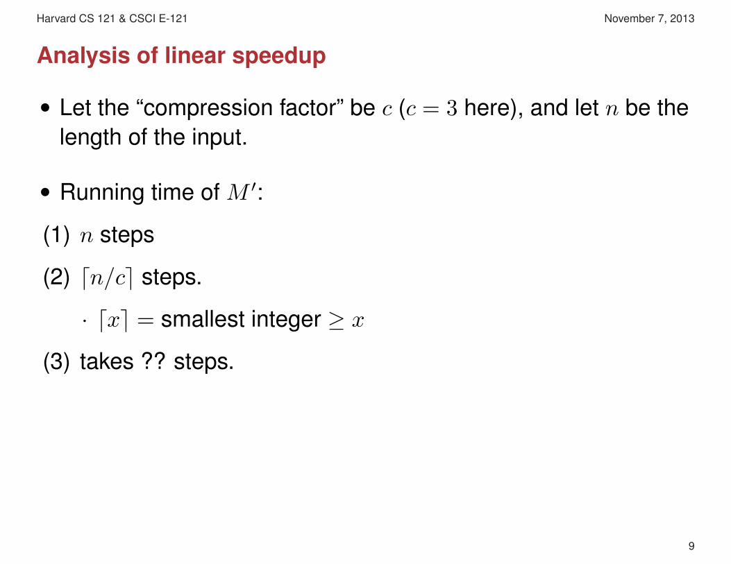
Analysis of linear speedup

• Let the “compression factor” be c (c = 3 here), and let n be thelength of the input.

• Running time of M ′:

(1) n steps

(2) dn/ce steps.

· dxe = smallest integer ≥ x

(3) takes ?? steps.

9


How long does the simulation (3) take?

• M ′ remembers in its finite control which of the c “subcells” M

is scanning.

• M ′ keeps simulating c steps of M by 8 steps of M ′:

(1) Look at current cell on either side.

(4 steps to read 3c symbols)

(2) Figure out the next c steps of M .

(can’t depend on anything outside these 3c subcells)

(3) Update these 3 cells and reposition the head.

(4 steps)

10


End of simulation analysis

• It must do this dt(n)/ce times, for a total of 8 · dt(n)/ce steps.

• Total of ≤ (10/c) · t(n) + n steps of M ′ for sufficiently large n.

• If c is chosen so that c ≥ 10/ε then M ′ runs in time ε · t(n) + n.

11


Implications/Rationalizations of Linear Speedup

• “Throwing hardware at a problem” can speed up any algorithmby any desired constant factor

• E.g. moving from 8 bit → 16 bit → 32 bit → 64 bit parallelism

• Our theory does not “charge” for huge capital expenditures tobuild big machines, since they can be used for infinitely manyproblems of unbounded size

• This complexity theory is too weak to be sensitive tomultiplicative constants — so we study growth rate

12


Growth Rates of Functions

We need a way to compare functions according to how fastthey increase not just how large their values are.

Def: For f : N → R+, g : N → R+, we write g = O(f) if thereexist c, n0 ∈ N such that g(n) ≤ c · f(n) for all n ≥ n0.

• Binary relation: we could write g = O(f) as g 4 f .

• “If f is scaled up uniformly, it will be above g at all but finitelymany points.”

• “g grows no faster than f .”

• Also write f = Ω(g).

13


Examples of Big-O notation

• If f(n) = n2 and g(n) = 1010 · n

g = O(f) since g(n) ≤ 1010 · f(n) for all n ≥ 0

where c = 1010 and n0 = 0

• Usually we would write: “1010 · n = O(n2)”

i.e. use an expression to name a function

• By Linear Speedup Theorem, TIME(t) is the class oflanguages L that can be decided by some multitape TM withrunning time O(t(n)) (provided t(n) ≥ 1.01n).

14


Examples

• 1010 · n = O(n2).

• 1764 = O(1).

1: The constant function 1(n) = 1 for all n.

• n3 6= O(n2).

• Time O(nk) for fixed k is considered “fast” (“polynomial time”)

• Time Ω(kn) is considered “slow” (“exponential time”)

• Does this really make sense?

15


Little-o and little-ω

Def: We say that g = o(f) iff for every ε > 0, ∃n0 such thatg(n) ≤ ε · f(n) for all n ≥ n0.

• Equivalently, limn→∞ g(n)/f(n) = 0.

• “g grows more slowly than f .”

• Also write f = ω(g).

16


Big-Θ

Def: We say that f = Θ(g) iff f = O(g) and g = O(f).

• “g grows at the same rate as f ”

• An equivalence relation between functions.

• The equivalence classes are called growth rates.

• Note: If limn→∞ g(n)/f(n) = c for some 0 < c < ∞, thenf = Θ(g), but the converse is not true. (Why?)

• Because of linear speed up, TIME(t) is really the union of allgrowth rate classes 4 Θ(t).

17


More Examples

Polynomials (of degree d):

f(n) = adnd + ad−1n

d−1 + · · ·+ a1n + a0, where ad > 0.

• f(n) = O(nc) for c ≥ d.

• f(n) = Θ(nd)

• “If f is a polynomial, then lower order terms don’t matter tothe growth rate of f ”

• f(n) = o(nc) for c > d.

• f(n) = nO(1). (This means: f(n) = ng(n) for some functiong(n) such that g(n) = O(1).)

18


More Examples

Exponential Functions: g(n) = 2nΘ(1).

• Then f = o(g) for any polynomial f .

• 2nα= o(2nβ

) if α < β.

What about nlg n = 2lg2 n?

Here lg x = log2 x

Logarithmic Functions:

loga x = Θ(logb x) for any a, b > 1

19


Asymptotic Notation within Expressions

When we use asymptotic notation within an expression, theasymptotic notation is shorthand for an unspecified functionsatisfying the relation.

• nO(1)

• n2 + Ω(n) means n/2 + g(n) for some function g(n) such thatg(n) = Ω(n).

• 2(1−o(1))n means 2(1−ε(n))·g(n) for some function ε(n) suchthat ε(n) → 0 as n →∞.

20


Asymptotic Notation on Both Sides

When we use asymptotic notation on both sides of anequation, it means that for all choices of the unspecifiedfunctions in the left-hand side, we get a valid asymptoticrelation.

• n2/2 + O(n) = Ω(n2) because for every function f such thatf(n) = O(n), we have n2/2 + f(n) = Ω(n2).

• But it is not true that Ω(n2) = n2/2 + O(n).

21

Harvard CS 121 and CSCI E-121 Lecture 19: Computational...

Documents

Transcript of Harvard CS 121 and CSCI E-121 Lecture 19: Computational...