1

Physics Letters A, Vol. 371, Nº 4, 291-299 (2007)

Harmonic balance approach to the periodic solutions of

the (an)harmonic relativistic oscillator

Augusto Beléndez and Carolina Pascual

Departamento de Física, Ingeniería de Sistemas y Teoría de la Señal.

Universidad de Alicante. Apartado 99. E-03080 Alicante. SPAIN

E-mail: a.belendez@ua.es

Corresponding author: A. Beléndez

Phone: +34-96-5903651

Fax: +34-96-5903464

2

ABSTRACT

The first-order harmonic balance method via the first Fourier coefficient is used to

construct two approximate frequency-amplitude relations for the relativistic oscillator for

which the nonlinearity (anharmonicity) is a relativistic effect due to the time line dilation

along the world line. Making a change of variable, a new nonlinear differential equation is

obtained and two procedures are used to approximately solve this differential equation. In

the first the differential equation is rewritten in a form that does not contain a square-root

expression, while in the second the differential equation is solved directly. The

approximate frequency obtained using the second procedure is more accurate than the

frequency obtained with the first due to the fact that, in the second procedure, application

of the harmonic balance method produces an infinite set of harmonics, while in the first

procedure only two harmonics are produced. Both approximate frequencies are valid for

the complete range of oscillation amplitudes, and excellent agreement of the approximate

frequencies with the exact one are demonstrated and discussed. The discrepancy between

the first-order approximate frequency obtained by means of the second procedure and the

exact frequency never exceeds 1.6%. We also obtained the approximate frequency by

applying the second order harmonic balance method and in this case the relative error is as

low 0.31% for all the range of values of amplitude of oscillation A.

Keywords: Nonlinear oscillations; Relativistic oscillator; Harmonic balance method;

Approximate frequency.

3

1. Introduction

The study of nonlinear oscillators is of great interest in engineering and physical

sciences and many analytical techniques have been developed for solving the second order

nonlinear differential equations that govern their motion [1]. It is difficult to solve

nonlinear differential equations and, in general, it is often more difficult to get an analytic

approximate than a numerical one of a given nonlinear oscillatory system [2]. There is a

large variety of approximate methods for the determination of solutions of nonlinear

second order dynamical systems including perturbation [3], standard and modified

Lindstedt-Poincaré [4-6], variational [7], variational iteration [8], homotopy perturbation

[9-12], harmonic balance [13-17] methods, etc. Surveys of the literature with numerous

references and useful bibliography and a review of these methods can be found in detail in

[2] and [18]. In this paper we apply the first-order harmonic balance method to obtain

analytic approximate solutions for the relativistic oscillator. This is a procedure for

determining analytical approximations to the periodic solutions of differential equations

by using a truncated Fourier series representation. This method can be applied to nonlinear

oscillatory systems where the nonlinear terms are not small and no perturbation parameter

is required.

When the energy of a simple harmonic oscillator is such that the velocities become

relativistic, the simple harmonic motion (linear oscillations) at low energy becomes

anharmonic (nonlinear oscillations) at high energy [19]. Due to this fact we have

considered the parentheses around the “an” in the title of this paper. Then, the strength of

the nonlinearity increases as the total relativistic energy increases, and at the non-

relativistic limit the oscillator becomes linear. Mickens [20] showed that all the solutions

to the relativistic (an)harmonic oscillator are periodic and determined a method for

calculating analytical approximations to its solutions. Mickens considered the first-order

harmonic balance method, but he did not apply the technique correctly and the first

analytical approximate frequency he obtained is not the correct one.

4

2. Nonlinear differential equation for the relativistic oscillator

The governing non-dimensional nonlinear differential equation of motion for the

relativistic oscillator is [20]

d2x

dt2

+ 1!dx

dt

"

# $

%

& '

2(

)

*

*

+

,

-

-

3 /2

x = 0 (1)

where x and t are dimensionless variables. The even power term in Eq. (1),

(dx / dt )2, acts

like the powers of coordinates in that it does not cause a damping of the amplitude of

oscillations with time. Therefore, Eq. (1) is an example of a generalized conservative

system [1]. At the limit when

(dx / dt )2<< 1, Eq. (1) becomes

(d2x / dt

2 ) + x ! 0 the

oscillator is linear and the proper time

! (

d! = 1" (dx / dt )2 dt ) becomes equivalent to

the coordinate time t to this order.

Introducing the phase space variable (x,y), Eq. (1) can be written as follows

dx

dt= y ,

dy

dt= !(1! y

2)3/ 2x (2)

and the trajectories in phase space are given by solutions to the first order, ordinary

differential equation

dy

dx= !

(1! y2)3/ 2x

y (3)

As Mickens pointed out, since the physical solutions of both Eq. (1) and Eq. (3) are real,

the phase space has a “strip” structure [20], i.e.,

!" < x < +" and

!1< y < +1 (4)

5

Then unlike the usual non-relativistic harmonic oscillator, the relativistic oscillator is

bounded in the y variable. This is due to the fact that the nondimensional variable y is

related with the relativistic relation

! = v /c , where v is the velocity of the particle and c

the velocity of light. In the relativistic case, the condition

!c < v(t ) < +c must be met, and

so we obtain

!1 < y(t ) < +1. Mickens proved that all the trajectories to Eq. (3) are closed

in the open region of phase space given by Eq. (4) and then all the physical solutions to

Eq. (1) are periodic. However, unlike the usual (non-relativistic) harmonic oscillator, the

relativistic (an)harmonic oscillator contains higher-order multiples of the fundamental

frequency.

In order to apply the harmonic balance method, we make a change of variable,

y! u, such that

!" < u < +", as follows

y =u

1+ u2

(5)

and the corresponding second order nonlinear differential equation for u is

d2u

dt2

+u

1+ u2

= 0 (6)

We consider the following initial conditions in Eq. (7)

u(0) = B anddu

dt(0) = 0 (7)

Eq. (6) is an example of conservative nonlinear oscillatory system having irrational

form for the restoring force. This is a conservative nonlinear oscillatory system and all the

motions corresponding to Eq. (6) are periodic [20], the system will oscillate symmetric

bounds [-B, B], and the angular frequency and corresponding periodic solution of the

nonlinear oscillator are dependent on the amplitude B.

6

The main objective of this paper is to solve Eq. (6) by applying the first-order

harmonic balance method and to compare the approximate frequency obtained with the

exact one and with another approximate frequency obtained by applying the method of

harmonic balance to the same oscillatory system but rewriting Eq. (6) in a way suggested

previously by Mickens [20]. Comparing with the approximate solution obtained by this

last procedure, the approximate frequency derived here is more accurate with respect to

exact solution. The errors of the resulting frequency are reduced and the maximum relative

error is less than 1.6% for the complete range of oscillation amplitudes, including the

limiting cases of amplitude approaching zero and infinity.

3. Solution method

3.1.- First adaptation of harmonic balance method

Eq. (6) is not amenable to exact treatment and, therefore, approximate techniques

must be resorted to. Eq. (6) can be rewritten in a form that does not contain the square-root

expression

(1+ u2)

d2u

dt2

!

"

#

$

%

&

2

= u2 (8)

It is possible to solve Eq. (8) by applying the method of harmonic balance.

Following the lowest order harmonic balance method, a reasonable and simple initial

approximation satisfying conditions in Eq. (7) can be taken as

u(t ) = Bcos!t (9)

The angular frequency of the oscillator is ω, which is unknown to be further determined.

The corresponding period of the nonlinear oscillation is given by T = 2π/ω. Both the

periodic solution u(t) and frequency ω (thus period T) depends on B. Substitution of Eq.

7

(9) into Eq. (8), and expanding and simplifying the resulting expression gives

1

2! 4

+3

8! 4

B2 "

1

2+

1

6! 4

B2 "

1

2

#

$ %

&

' ( + (higher " order harmonics) = 0 (10)

and setting the coefficient of the resulting term

cos(0! t) (the lowest harmonic) equal to

zero gives the first analytical approximate frequency

!a1

as a function of B

!a1(B) = 1+

3

4B

2"

# $

%

& '

(1/ 4

(11)

which is valid for the whole range of values of B. By applying the first order homotopy

perturbation method to Eq. (8) the same approximate frequency is obtained [21] and this is

due to the fact that in both methods the first Fourier coefficient is obtained. We can

conclude that this is a general result for conservative oscillators. The approximate

frequency in Eq. (11) is the correct one when the harmonic balance method is applied to

Eq. (8), and not the frequency obtained in Ref. [20].

3.2.- Second adaptation of harmonic balance method

As we pointed out previously, the main objective of this paper is to solve Eq. (6)

instead of Eq. (8) by applying the harmonic balance method. Substitution of Eq. (9) into

Eq. (6) gives

!B"2

cos"t +Bcos"t

1+ cos2"t

= 0 (12)

The power-series expansion of

u / 1+ u2 is

u

1+ u2

= u + (!1)n (2n !1)!

22n!1n!(n !1)!n=1

"

# u2n+1 (13)

8

Substituting Eq. (13) into Eq. (12) and taking into account Eq. (9) gives

(!"2+ 1)cos"t + (!1)n (2n !1)!

22n!1n!(n !1)!n=1

#

$ B2n cos2n+1

"t = 0 (14)

The formula that allows us to obtain the odd power of the cosine is

cos2n+1!t =1

22n

2n + 1

n

"

# $

%

& ' cos!t +

2n + 1

n (1

"

# $

%

& ' cos3!t + … +

2n + 1

0

"

# $

%

& ' cos[(2n + 1)!t]

)

*

+

,

-

.

(15)

Substituting Eq. (15) into Eq. (16) gives

!"2+ c2n+1

n=0

#

$ B2n

%

&

'

'

(

)

*

* cos"t + (higher ! order harmonics) = 0 (16)

where the coefficients c2n+1 are given by

c1 = 1 (17)

and

c2n+1 = (!1)n (2n !1)!(2n + 1)!

24n!1(n!)2(n !1)!(n + 1)! for n ≥ 1 (18)

For the lowest order harmonic to be equal to zero, it is necessary to set the

coefficient of cosωt equal to zero in Eq. (16), then

!(B) = c2n+1

n=0

"

# B2n

$

%

& &

'

(

) )

1/2

(19)

In order to obtain the value of

c2n+1

n=0

!

" B2n in Eq. (19) we consider the following relations

9

(2n !1)!

22n!1(n !1)!= 1/ 2( )

n ,

(2n + 1)!

22nn!

= 3/ 2( )n,

(n + 1)!= (2)n (20)

where (a)n is the Pochhammer symbol [22]

(a)n

= a(a + 1)…(a + n !1) (21)

Taking into account Eqs. (17), (20) and (21) it is possible to write

c2n+1

n=0

!

" B2n as follows

c2n+1

n=0

!

" B2n

=1/ 2( )

n

3/ 2( )n

(2)n

(#B2)n

n!n=0

!

" = 2F11

2,3

2;2;#B

2$

% &

'

( ) (22)

where

2 F1 a , b;c; z( ) is the hypergeometric function [22]

2 F1 a ,b;c; z( ) =(a)n(b)n

(c)nn=1

!

"z

n

n! (23)

Substituting Eq. (22) into Eq. (19) gives

!b1(B) =

2F

1

1

2,3

2;2;"B2#

$ %

&

' (

)

* +

,

- .

1/2

(24)

which is the angular frequency obtained applying the low-order harmonic balance method

directly to Eq. (6). By the software MATHEMATICA, we can readily obtain the following

relation

!b1(B) =

2F

1

1

2,3

2;2;"B2#

$ %

&

' (

)

* +

,

- .

1/2

=2

/BE("B2

) "K("B2)[ ]

1/2

(25)

To obtain Eq. (25), the command “FunctionExpand” has been applied to

10

2F

11/2,3/2;2;!B

2( ) . K(m) and E(m) are the complete elliptic integrals of the first and

second kind, respectively, defined as follows [23]

K(m) =d!

1"mcos2!0

# /2$ (26)

E(m) = 1!mcos2" d"0

# /2$ (27)

By applying the first order homotopy perturbation method to Eq. (6), the same

approximate frequency is obtained [24].

The corresponding approximation to y is obtained from Eqs. (5) and (9)

y(t ) =u(t )

1+ u2(t )

=Bcos!t

1+ B2 cos2

!t (28)

Likewise,

x(t ) can be calculated by integrating equation

y = dx /dt subject to the

restrictions

x(0) = 0, y(0) =B

1+ B2

(29)

which can be easily obtained from Eqs. (5) and (7). This integration gives

x j(t ) =1

! j (B)sin"1 B

1+ B2

sin[! j(B)t]#

$

%

%

&

'

(

(

, j = 1, 2 (30)

However, we should not forget what we are really looking for is an approximate analytical

solution to Eq. (1), that is, x(t). Moreover, it is convenient to express the approximate

angular frequency and the solution in terms of oscillation amplitude A rather than as a

11

function of B. It is now necessary to find a relation between oscillation amplitude A and

parameter B used to solve Eqs. (6) and (8) approximately. From Eq. (3) we get

1

(1! y2 )1/2

+1

2x

2= C (31)

where C is a constant to be determined as a function of initial conditions. From Eq. (28)

we can easily obtain

C = (1+ B2)1/ 2 and Eq. (31) can be written as follows

1

(1! y2 )1/2

+1

2x

2= (1+ B

2 )1/2 (32)

In addition, when x = A, the velocity

y = dx /dt is zero. Taking this into account in

Eq. (32), we obtain the following relation between amplitude A and parameter B

1+1

2A

2= (1+ B

2 )1/2 (33)

From the above equation we can easily find that the solution for B is

B = A 1+1

4A

2!

" #

$

% &

1/2

(34)

Substituting Eq. (34) into Eqs. (11), (26) and (29), the first analytical approximate

periodic solutions for the relativistic oscillator as a function of the oscillation amplitude A

are given by

!a1(A) = 1+

3

4A

2+

3

16A

2"

# $

%

& '

(1/ 4

(35)

12

!b1(A) =

4

A "(4 + A2)E #

1

4A

2(4 + A

2)

$

% &

'

( ) #K #

1

4A

2(4 + A

2)

$

% &

'

( )

*

+ ,

-

. /

1/2

(36)

x j(t ) =1

! j ( A)sin"1 4A

2+ A

4

4 + 4A2

+ A4

sin[! j ( A)t]

#

$

%

%

&

'

(

( , j = a1, b1 (37)

3.3.- Results and discussion

In this section we illustrate the accuracy of the proposed approach by comparing

the approximate frequencies ωa1(B) and ωb1(B) obtained in this paper with the exact

frequency ωex(A). The exact angular frequency is calculated as follows. Substituting Eq.

(34) into Eq. (32), we obtain

1

(1! y2 )1/2

=1

2( A

2! x

2 ) (38)

The exact frequency can then be derived as follows

!ex

( A) ="

2

1+ 1

2( A

2 - x2 )

A2 - x

2 + 1

4( A

2 - x2 )20

A

# dx

$

%

&

&

'

(

)

)

*1

(39)

which can be written in terms of elliptical integrals as follows

!ex

( A) = 2" 4 4 + A2E

A2

4 + A2

#

$

% %

&

'

( ( )

8

4 + A2

KA

2

4 + A2

#

$

% %

&

'

( (

*

+

,

,

-

.

/

/

)1

(40)

where K(m) and E(m) are the complete elliptic integrals of the first and second kind,

respectively, defined in Eqs. (26) and (27).

For small values of the amplitude A it is possible to take into account the following

approximation,

13

!ex

( A) "1#3

16A

2+

51

1024A

4#

233

16384A

6+ … (41)

For small values of A it is also possible to do the power-series expansion of the

approximate angular frequencies ωa1 (Eq. (35)) and ωb1 (Eq. (36)). In this way the

following equations can be obtained

!a1(A) "1#

3

16A

2+

42

1024A

4#

90

16384A

6+ … (42)

!b1(A) "1#

3

16A

2+

54

1024A

4#

278

16384A

6+ … (43)

These series expansions were carried out using MATHEMATICA. As can be seen,

in the expansions of the angular frequencies, ωa1 (Eq. (42)) and ωb1 (Eq. (43)), the first two

terms are the same as the first two terms of the equation obtained in the power-series

expansion of the exact angular frequency, ωex (Eq. (41)). By comparing the third terms in

Eqs. (42) and (43) with the third term in the series expansion of the exact frequency ωex

(Eq. (41)), we can see that the third term in the series expansions of ωb1 (Eq. (43)) is more

accurate than the third term in the expansion of ωa1 (Eq. (42)).

Now we are going to obtain an asymptotic representation for large amplitudes. For

very large values of the amplitude A it is possible to take into account the following power

series expansions

!ex

( A) "#

2A+ … =

1.57080

A+ … (44)

!a1(A) "

2

31/ 4A

+ … =1.51967

A+ … (45)

14

!b1(A) "

8

#

1

A+ … =

1.59577

A+ … (46)

Once again we can also see than the frequency

!b1(A) is more accurate than

!a1(A) and

can provide excellent approximations to the exact frequency

!ex

( A) for very large values

of oscillation amplitude. Now, the relative errors of the first term of series expansions of

!a1(A) and

!b1(A) are 3.3% and 1.6%, respectively. These results confirm the fact that

ωb1 is a better approximation to the exact frequency ωex than the approximate frequency

ωa1, not only for small amplitudes but also for large values of the amplitude of oscillation.

The exact periodic solutions x(t) achieved by numerically integrating Eq. (1), and

the proposed normalized first-order approximate periodic solutions x1(t) and x2(t) in Eq.

(37), respectively, for one complete cycle are plotted in Figures 1 and 2 for A = 1 and 10,

respectively. In these figures parameter h is defined as follows

h = Tex

( A)t =2!t

"ex

( A) (48)

As the dimensionless variable y is equal to v/c, where v and c are the velocity of the

particle and the velocity of light, respectively,

!0 =v0

c= y(0) =

B

1+ B2

=4 A

2+ A

4

4 + 4 A2

+ A4

(49)

Figures 1 and 2 show that Eq. (37) provides a good approximation to the exact

periodic solution and it is adequate to obtain the approximate analytical expression of x(t).

As we can see, for small values of A (Figure 1) x(t) is very close to the sine function form

of nonrelativistic simple harmonic motion. For higher values of A (Figure 2) the curvature

becomes more concentrated at the turning points

(x = ±A). For these values of A, x(t)

becomes markedly anharmonic and is almost straight between the turning points. Only in

the vicinity of the turning points, where the magnitude of the Hooke’s law force is

15

maximum and the velocity becomes relativistic, is the force effective in changing the

velocity [19]. Figure 2 is typical example of the motion in the ultrarelativistic region

where

!0"1.

At this point it is necessary to answer the following questions: (a) why does

substitution of Eq. (9) into Eq. (6) not give the same result as substitution of Eq. (9) into

Eq. (8)?, and (b) why does application of the first-order harmonic balance method to Eq.

(6) give a more accurate frequency than application of the method to Eq. (8)? These

questions have been analyzed in detail in reference [24] and here we are going only to

summarize the results. If we substitute Eq. (9) into Eq. (8) and we divide the resulting

equation by cosωt we obtain an equation that includes only two odd powers of cosωt,

cosωt and cos3ωt, and then there are only two contributions to the coefficient of the first

harmonic cosωt, which are 1 from cosωt and 3/4 from cos3ωt. Therefore, substituting Eq.

(9) into Eq. (8) produces only the first harmonic, cosωt, and the third harmonic, cos3ωt,

! 41+

3

4B

2"

# $

%

& ' (1

)

*

+

,

-

. cos!t +1

4! 4

B2

cos3!t = 0 (50)

However, Eq. (14) includes all odd powers of cosωt, which are cos2n+1ωt with n =

0, 1, 2, …, ∞, and then there are infinite contributions to the coefficient of the first

harmonic cosωt, that is, 1 from cosωt, 3/4 from cos3ωt, 5/8 from cos5ωτ, …,

2!2n 2n + 1

n

"

# $

%

& '

from

cos2n+1

!t , and so on. Therefore, substituting Eq. (9) into Eq. (6) produces the

infinite set of higher harmonics, cosωt, cos3ωt, …, cos[(2n+1)ωt], and so on. Similar

phenomenon occurred in [10] and [15] for the Duffing-harmonic oscillator.

It can be seen that Eqs. (11) and (25) have the form

! j (B)= f j (B)[ ] "1/ 4 , j = a1, b1 (51)

which allows the approximate frequency ω to be determined in terms of the oscillation

16

amplitude B. From this equation we can conclude that application of the first-order

harmonic balance method to Eqs. (6) and (8) gives the same functional form for the

approximate frequency ω. The difference between these approximate frequencies is the

function f(B)

!a1(B) = 1+

3

4B

2"

# $

%

& '

(1/ 4

and

fa1(B) = 1+

3

4B

2 (52)

!b1(B) =

2F

1

1

2,3

2;2;"B2#

$ %

&

' (

"2#

$

%

&

'

(

"1/ 4

and

fb1(B)=

2F

1

1

2,3

2;2;!B2"

# $

%

& '

!2

(53)

If we do the power-series expansion of

2F

11/2,3/2;2;!B

2( )!2

we have

!b1(B) = 1+

3

4B

2 "3

64B

4+

13

512B

6+ …

#

$ %

&

' (

"1/ 4

(54)

As can be seen, in this equation the first two terms in the brackets are identical to the two

terms in brackets in Eq. (52); whereas powers B4, B6,… are due to the infinite set of

higher harmonics in Eq. (14). Applying the harmonic balance method to Eqs. (6) and (9)

with higher harmonics, the two procedures will give more accurate results. In the limit in

which we include all the harmonics, they must give us exactly the same solution, since Eq.

(9) is equivalent to Eq. (6).

4. Higher order approximation

As the application of the first-order harmonic balance method to Eq. (6) give a

more accurate frequency than application of the method to Eq. (8), we have obtain the

second order approximation for Eq. (6). The next level of harmonic balance uses the form

[16]

17

u2(t ) = u1(t ) + !u1(t ) (55)

where

u1(t) = Bcos!t (Eq. (9)) and

!u1(t ) is the correction part. Substituting Eq. (55)

into Eq. (6) and linearizing the resulting equation with respect to the correction

!u1(t ) at

u(t) = u1(t) leads to

d2u

1

dt2

+d

2!u

1

dt2

+u

1

1+ u1

2+

!u1

(1+ u1

2)

3 /2= 0 (56)

and

!u1(0) = 0,d!u1

dt(0) = 0 (57)

To obtain the second approximation to the exact solution,

!u1(t ) in Eq. (55),

which must satisfy the initial conditions in Eq. (57), takes the form

!u1 = c1(cos"t # cos3"t ) (58)

where

c1 is a constant to be determined. Substituting Eqs. (9), (55) and (58) into Eq. (56),

expanding the expression in a trigonometric series and setting the coefficients of the

resulting items

cos!t and

cos3!t equal to zero, respectively, yield

!(B + c1)B

4"

2# 4(B

3# 8c

1)E(#B

2) + 4(B

3# 8c

1# 4c

1B

2)K(#B

2) = 0 (59)

and

27!c1B

6"

2# 4(8B

3+ B

5#128c

1# 88c

1B

2)E(#B

2)

+ 4[(B3(8 + 5B

2) # 4(32 + 38B

2+ 9B

4)c

1]K(#B

2) = 0

(60)

From Eq. (29) we can obtain the second analytical approximate frequency

!b2

as

follows

18

!b2(B) =

4(B3 " 8c

1)E("B2

) " 4(B3 " 8c

1" 4c

1B

2)K("B2

)

#(c1

+ B)B4

$

%

&

'

(

)

1/2

(61)

Substituting Eq. (61) into Eq. (60) and solving for

c1, we obtain

c1

=B

5[(8 + B

2)E(!B

2) ! (8 + 5B

2)K(!B

2)]

("1

+ "2)1/2B

2+ (64B

2+ 40B

4+ 13B

6)E(!B

2) ! (64B

2+ 72B

4+ 29B

6)K(!B

2)

(61)

where

!1

= [("64 " 48B2

+ 13B4)E("B

2) + (64 + 80B

2+ 7B

4)K("B

2)]

2 (62)

!2

= "432B4["(4 + 5B

2)E

2("B

2) " 2(4 + 5B

2+ B

4)E("B

2)K("B

2) " (4 + 5B

2+ B

4)K

2("B

2)]

(63)

For small values of the amplitude A it is possible to take into account the following

power series expansion of the second order approximate angular frequency

!b2(A) "1#

3

16A

2+

51

1024A

4#

238.25

16384A

6+ … (64)

where we have taken into account Eq. (34). As can be seen, in the expansion of the

angular frequency

!b2(A) , the first three terms are the same as the first three terms of the

equation obtained in the power-series expansion of the exact angular frequency,

!ex

( A)

(Eq. (41)). For very large values of the amplitude A it is possible to take into account the

following power series expansion

19

!b2(A) "

1.5659

A+ … (65)

Once again we can see than

!b2(A) provides excellent approximations to the exact

frequency

!ex

( A) for very large values of oscillation amplitude and the relative error for

!2b(A) is lower than 0.31% for all the range of values of amplitude of oscillation A.

6. Conclusions

The first order harmonic balance method was used to obtain two approximate frequencies

for the relativistic oscillator in which the restoring force has an irrational form. An

approximate frequency, ωa1, was obtained by rewriting the nonlinear differential equation

in a form that does not contain an irrational expression; while the second one, ωb1, was

obtained by solving the nonlinear differential equation containing a square-root expression

approximately. We can conclude that formulas (35) and (36) are valid for the complete

range of oscillation amplitude, including the limiting cases of amplitude approaching zero

and infinity. Excellent agreement of the approximate frequencies with the exact one was

demonstrated and discussed and the discrepancy between the first order approximate

frequency, ωb1, and the exact one never exceeds 1.6%. The first order approximate

frequency, ωb1, derived here is the best frequency that can be obtained using the first-order

harmonic balance method, and the maximum relative error was significantly reduced as

compared with the first approximate frequency, ωa1. We have also shown that applying the

first order harmonic balance method to Eqs. (6) and (8) we obtain the same results that

those obtained by applying the first order homotopy perturbation method to Eqs. (6) and

(8). We can conclude that this is a general result for conservative oscillators. Some

examples have been presented to illustrate excellent accuracy of the approximate

analytical solutions. We discussed the reason why the accuracy of the approximate

frequency, ωb1, is better than that of the frequency, ωa1. This reason is related to the

number of harmonics that application of the first-order harmonic balance method produces

20

for each differential equation solved, two harmonics for the first case and the infinite set of

harmonics for the second one. We also obtained the approximate frequency

!2b(A) by

applying the second order harmonic balance method to Eq. (6) and we obtained that the

relative error for

!2b(A) is lower than 0.31% for all the range of values of amplitude of

oscillation A.

Finally, we can see that the method considered here is very simple in its principle,

and is very easy to apply.

Acknowledgements

This work was supported by the “Ministerio de Educación y Ciencia”, Spain, under project

FIS2005-05881-C02-02, and by the “Generalitat Valenciana”, Spain, under project

ACOMP/2007/020.

21

References

[1] R. E. Mickens, Oscillations in Planar Dynamics Systems (World Scientific,

Singapore 1996).

[2] J. H. He, Non-perturbative methods for strongly nonlinear problems

(dissertation.de-Verlag im Internet GmbH, Berlin 2006).

[3] A. H. Nayfeh, Problems in Perturbations (Wiley, New York 1985).

[4] P. Amore, A. Raya and F. M. Fernández, “Alternative perturbation approaches in

classical mechanics”, European Journal of Physics 26, 1057-1063 (2005).

[5] P. Amore. A. Raya and F. M. Fernández, “Comparison of alternative improved

perturbative methods for nonlinear oscillations”, Physics Letters A 340, 201-208

(2005).

[6] J. H. He, “Modified Lindstedt-Poincare methods for some non-linear oscillations.

Part I: expansion of a constant”, Int. J. Non-linear Mech. 37, 309-314 (2002).

[7] J. H. He, “Variational approach for nonlinear oscillators”, Chaos, Solitons &

Fractals 34, 1430-1439 (2007).

[8] J. H. He and X. H. Wu, “Construction of solitary solution and compacton-like

solution by variational iteration method”, Chaos, Solitons & Fractals 29, 108-113

(2006).

[9] J. H. He, “Homotopy perturbation method for bifurcation on nonlinear problems”,

Int. J. Non-linear Sci. Numer. Simulation. 6, 207-208 (2005).

[10] A. Beléndez, A. Hernández, T. Beléndez, E. Fernández, M. L. Álvarez and C.

Neipp, “Application of He’s homotopy perturbation method to the Duffing-

harmonic oscillator”, International Journal of Non-linear Sciences and Numerical

Simulation 8 (1), 79-88 (2007).

22

[11] J. H. He, “Homotopy perturbation method for solving boundary value problems”,

Physics Letters A 350, 87-88 (2006).

[12] A. Beléndez, A. Hernández, T. Beléndez, C. Neipp and A. Márquez, “Application of

the homotopy perturbation method to the nonlinear pendulum”, European Journal of

Physics 28, 93-104 (2007).

[13] R. E. Mickens, “Comments on the method of harmonic-balance”, Journal of Sound

and Vibration 94, 456-460 (1984).

[14] A. Beléndez, A. Hernández, A. Márquez, T. Beléndez and C. Neipp, “Analytical

approximations for the period of a simple pendulum”, European Journal of Physics

27, 539-551 (2006).

[15] H. Hu and J. H. Tang, “Solution of a Duffing-harmonic oscillator by the method of

harmonic balance”, Journal of Sound and Vibration 294, 637-639 (2006).

[16] C. W. Lim and B. S. Wu, “A new analytical approach to the Duffing-harmonic

oscillator”, Physics Letters A 311, 365-373 (2003).

[17] A. Beléndez, A. Hernández, T. Beléndez, M. L. Álvarez, S. Gallego, M. Ortuño and

C. Neipp, “Application of the harmonic balance method to a nonlinear oscillator

typified by a mass attached to a stretched wire”, Journal of Sound and Vibration

302, 1018-1029 (2007).

[18] J. H. He, “Some asymptotic methods for strongly nonlinear equations”, International

Journal of Modern Physics B 20, 1141-1199 (2006).

[19] W. Moreau, R. Easther and R. Neutze, “Relativistic (an)harmonic oscillator”, Am. J.

Phys. 62, 531-535 (1994).

[20] R. E. Mickens, “Periodic solutions of the relativistic harmonic oscillator”, Journal of

Sound and Vibration 212, 905-908 (1998).

23

[21] A. Beléndez, C. Pascual, A. Márquez and D. I. Méndez, “Application of He’s

Homotopy Perturbation Method to the Relativistic (An)harmonic Oscillator. I:

Comparison between Approximate and Exact Frequencies”, International Journal of

Non-linear Sciences and Numerical Simulation 8 (4), (2007). –in press-

[22] F. Oberhettinger, “Hypergeometric functions” in M. Abramowitz and I. A. Stegun

(Eds.), Handbook of Mathematical Functions, Dover Publications, Inc., New York,

1972.

[23] L. M. Milne-Thomson, “Elliptic integrals” in M. Abramowitz and I. A. Stegun

(Eds.), Handbook of Mathematical Functions, Dover Publications, Inc., New York,

1972.

[24] A. Beléndez, C. Pascual, D. I. Méndez, M. L. Álvarez and C. Neipp, “Application of

He’s Homotopy Perturbation Method to the Relativistic (An)harmonic Oscillator. II:

A More Accurate Approximate Solution”, International Journal of Non-linear

Sciences and Numerical Simulation 8 (4), (2007). –in press-

24

FIGURE CAPTIONS

Figure 1.- Comparison of the analytical approximate solutions

x1 (black circles) and

x2

(white circles) with the exact solution (continuous line) for A = 1

(!0 = v0 / c = 0.74536).

Figure 2.- Comparison of the analytical approximate solutions

x1 (black circles) and

x2

(white circles) with the exact solution (continuous line) for A = 10

(!0 = v0 / c = 0.99981).

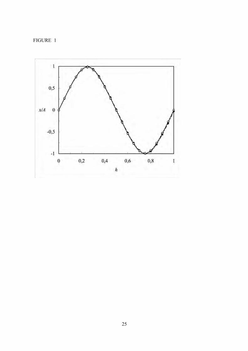
25

FIGURE 1

26

FIGURE 2