Hark! Who goes there? Concurrent Association of...

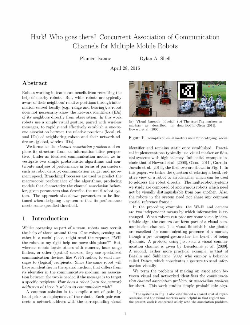
Hark! Who goes there? Concurrent Association of Communication

Channels for Multiple Mobile Robots

Plamen Ivanov Dylan A. Shell

April 28, 2016

Abstract

Robots working in teams can benefit from recruiting thehelp of nearby robots. But, while robots are typicallyaware of their neighbors’ relative positions through infor-mation sensed locally (e.g., range and bearing), a robotdoes not necessarily know the network identifiers (IDs)of its neighbors directly from observation. In this workrobots use a simple visual gesture, paired with wirelessmessages, to rapidly and effectively establish a one-to-one association between the relative positions (local, vi-sual IDs) of neighboring robots and their network ad-dresses (global, wireless IDs).

We formalize the channel association problem and ex-plore its structure from an information filter perspec-tive. Under an idealized communication model, we in-vestigate two simple probabilistic algorithms and con-tribute analyses of performance in terms of parameters,such as robot density, communication range, and move-ment speed, Branching Processes are used to predict themacroscopic performance of the algorithms, producingmodels that characterize the channel association behav-ior, given parameters that describe the multi-robot sys-tem. The approach also allows parameters to be fine-tuned when designing a system so that its performancemeets some specified threshold.

1 Introduction

Whilst operating as part of a team, robots may recruitthe help of those around them. One robot, sensing an-other in a useful place, might send the request: “Willthe robot to my right help me move this piano?” But,whereas robots locate others with cameras, laser rangefinders, or other (spatial) sensors, they use specializedcommunication devices, like Wi-Fi radios, to send mes-sages to (logical) recipients. Since the same robot willhave an identifier in the spatial medium that differs fromits identifier in the communicative medium, an associa-tion between the two is needed if the message is to targeta specific recipient. How does a robot learn the networkaddresses of those it wishes to communicate with?

A common solution is to compile a set of pairs byhand prior to deployment of the robots. Each pair con-nects a network address with the corresponding visual

(a) Visual barcode fiducialmarkers as described inHoward et al. [2006].

(b) The AprilTag markers asdescribed in Olson [2011].

Figure 1: Examples of visual markers used for identifying robots.

identifier and remains static once established. Practi-cal implementations typically use visual marker or fidu-cial systems with high saliency. Influential examples in-clude that of Howard et al. [2006], Olson [2011], Garrido-Jurado et al. [2014], the first two are shown in Fig. 1. Inthis paper, we tackle the question of relating a local, rel-ative view of a robot to an identifier which can be usedto address the robot directly. The multi-robot systemswe study are composed of anonymous robots which neednot be visually distinguishable from one another. Also,the robots in the system need not share any commonspatial reference frame.1

In the preceding examples, the Wi-Fi and cameraare two independent means by which information is ex-changed. When robots can produce some visually iden-tifiable sign, the camera can form part of a visual com-munication channel. The visual fiducials in the photosare excellent for communicating presence of a marker,though a pre-arranged gesture has the benefit of beingdynamic. A protocol using just such a visual commu-nication channel is given by Dieudonne et al. [2009].A second, rather more practical example, is that ofBatalin and Sukhatme [2002] who employ a behaviorcalled Dance, which constitutes a gesture to send infor-mation visually.

We term the problem of making an association be-tween visual and networked identifiers the communica-tion channel association problem, or association problemfor short. This work studies simple probabilistic algo-

1The systems in Fig. 1 also established a shared spatial repre-sentation and the visual markers were helpful in that regard too—the present work is concerned solely with the association problem.

1

rithms that solve the association problem without rely-ing on global information or external markers. Instead,the robots use a simple, visually identifiable gesture (likea light being turned on-and-off or a Dance behavior) andwireless communication to solve the association problemquickly and concurrently. The identifiers of robots in thevisual channel (visual IDs) are locally assigned by eachobserver (it is helpful to think of the typical, represen-tative case of the IDs being the range and bearing toeach visible robot). The network IDs of the robots inthe wireless channel are assigned to the robots globallyand do not depend on other robots’ perspectives.

This paper’s focus is on understanding and predict-ing the expected behavior of this association process forlarge multi-robot systems. We analyze the problem us-ing an idealized model of the inter-agent communica-tion, which enables characterization of the performancein terms of very few parameters. Starting with simula-tions, three key system parameters were identified: robotdensity, communication range, and robot velocity. Theeffect that each has on performance is examined in detail,and a model using the theory of Branching Processes topredict the expected macroscopic performance of suchsystems constructed.

The paper is organized as follows. Section 2 exam-ines related work. In Section 3 we formalize the com-munication channel association problem, describing thecommunication model we study, and introducing the in-formation space view. Section 4 addresses the problemwith stationary robots and then, Section 5, the mobilecase. The models are validated by comparing their pre-dictions to the simulation results. We also show that aMarkov chain analysis is infeasible when applied to theassociation problem. The infeasibility of standard anal-ysis, even under assumptions of perfect communication,helps exculpate the simplified model we employ. But,because the results obtained are for this idealized com-munication model, they may be best viewed as bounds forsystems involving erroneous packet transmissions. Nev-ertheless, Section 6 returns to our modeling assumptions,suggesting that several real-world circumstances are ap-proximated reasonably well. Section 7 concludes.

2 Related Work and Background

2.1 Related Work

The notion of situated communication is central to solv-ing the channel association problem. Støy [2001] distin-guishes abstract channels, which carry meaning only inthe message contents, from situated channels. In situatedcommunication some property, inherent to the channel,provides additional meaning to the received messages.In our case, the visual channel is situated and the addedinformation is the relative position of the transmitter. Amore general concept, encompassing the situated prop-erty, is that of indexical knowledge [Agre and Chapman,

1987, Lesperance and Levesque, 1995]. Indexical knowl-edge refers to knowledge, which is relative to the ob-server. It is contrasted by objective knowledge, which isindependent from the perspective of the observer.

One may categorize robotic systems informally basedon the number of communication channels that areavailable to them. Most common are one- and two-channel systems (e.g. idealized wireless in the first case,and infrared communication devices in the second). InDieudonne et al. [2009], the authors examine a sce-nario where the robots can only communicate throughmovement-signals. Their work shows how an explicitcommunication channel can be established using robotsensors and robot gestures — the gestures consist of spe-cific motion of a robot through the environment.

A multi-robot system falls under the two-channel cat-egory if its robots are equipped with two independentcommunication devices such as wireless and infrared-based communication. In such systems, typically, bothcommunication channels are capable of transmitting arobot’s ID reliably. In addition, the infrared communi-cation channel is also a situated one, it can be used todetect range and bearing to other robots (cf. Gutierrezet al. [2008]). Since each channel can transmit a robot’sID, this means that the association problem can besolved by directly sending a message containing the ID.Robots which receive the message now know the robot’sidentity and can address them directly in either channel.

As Dieudonne et al. [2009] and Batalin and Sukhatme[2002] show, a communication channel can be establishedthrough the use of any robot sensor which can detect achange in the state of another robot. In our work, thesecond communication channel is assumed to be estab-lished through a camera and a light (vision beacon).

Multi-robot systems in which there is no explicitsecond communication channel, such as Howard et al.[2006], Garrido-Jurado et al. [2014], Olson [2011], muststill solve the association problem. As mentioned above,a common approach in such systems is to use passivemarkers along with a fixed pre-compiled list of marker-network address pairs. This sort of static association hasthe limitation of requiring maintenance by some mech-anism external to the multi-robot system. Additionally,such markers can encode a limited number of uniqueidentifiers, may suffer from reliability issues, and mayimpose restrictions on the maximum distance at whichthe markers can be identified. Markers may also increasethe computational or hardware required by the system.

This work addresses algorithmic aspects of the asso-ciation problem for systems where the second channeldoes not suffice to transmit IDs directly. Most closelyrelated is the recent work of Mathews et al. [2012, 2015]which introduces the concept of spatially targeted com-munication. They use the idea of a situated channel totarget communication to a receiver based on their lo-cation in space. Both the model and solution in theirwork have similarities with that which we describe be-

2

low. But their work establishes an association betweena pair of robots in the system, while we establish an as-sociation between all robots in the system concurrentlyand without restricting the use of the wireless and visualcommunication channels for any robot.

Finally, we note that mutual or collective localizationin a multi-robot system, as exemplified by Franchi et al.[2009] and Fox et al. [2000] is related to the associationproblem because it solves a harder problem, the solu-tion to which can provide a common reference frame forrobots in a system. However, the cost of localization ofall robots may be greater than is desirable simply fortargeted communication.

2.2 Background

The information space and information state conceptsexplained by LaValle [2009] underpin our understandingof the association process. An information state encap-sulates the abstract information which a robot maintainsto keep track of the world around it. The informationspace can be seen as the set of all information statesand a transition function which describes how one in-formation state is transformed into another, given anobservation.

We also use techniques based on discrete-time absorb-ing Markov chain [Berend and Tassa, 2010] and discrete-time Branching Processes [Haccou et al., 2007] to analyzeand predict the macroscopic behavior of a multi-robotsystem solving the association problem.

An earlier version of this work appeared in our confer-ence paper, Ivanov and Shell [2014]. This paper expandsthe analysis substantially and offers an extended algo-rithm for solving the association problem for a systemcomposed of mixture of stationary and mobile robots.

3 General Description of the As-sociation Problem

Consider a large number of robots spread randomlyand uniformly through an open and empty environment.Each robot in the system can directly observe (and dis-tinguish from the environment) other robots using acamera or array of cameras with a 360 field of view.The robots’ operation proceeds in discrete, synchronoustime steps. Each robot has a light which can be on or offduring any time step. The camera and light form a situ-ated visual communication channel and robots may alsobroadcast messages through a wireless channel. Bothchannels have limited range. Every robot is assigned awireless ID and itself assigns visual IDs to robots it candetect with its camera. The following is a list of assump-tions about the motivating system.

Assumption 1. Perfect communication: Messages areneither lost, degraded, nor noisy. A message broadcast

by a robot will be received by all robots within rangeduring the time step it was transmitted.

Assumption 2. Message size: The wireless communi-cation medium can transmit the full binary representa-tion of a robot’s ID: log2(n) bits. The visual channel cantransmit a message of size 1 bit.

Assumption 3. Unlimited bandwidth and message pro-cessing: Robots can receive and process any number ofmessages during each time step.

The preceding, idealized model describes the systemused in our simulation experiments and serves as thebasis of our formal model as well as subsequent anal-ysis. Observe that we do not consider communicationerrors or robot failures. Section 6.3 discusses potentialapproaches for dealing with communication noise and er-ror while Section 6.4 provides an informal discussion onthe feasibility of Assumption 3.

3.1 Formal Definition

Definition 1. We consider a multi-robot system ofrobots capable of communicating via a radio communica-tion channel (channel 1) and a physically situated com-munication channel (channel 2), and described by a tu-ple: 〈G1 = 〈V,E1〉, G2 = 〈V,E2〉, C1, C2, f1, f2〉 where

1. V is a set of vertices, each vertex represents a robot.

2. G1 = 〈V,E1〉 and G2 = 〈V,E2〉 are two directedgraphs representing the connectivity of the systemover the two channels. Edge e ≡ (vi, vj) ∈ Ek is in-terpreted as robot i being able to receive a one-hopmessage from robot j over communication channel k.

3. E2 ⊆ E1 — This is Property 2 (see below).

4. C1 and C2 are the label sets for channels 1 and 2.

5. f1, f2 are labeling functions f : V × V → C whichare applied to channels 1 and 2, respectively. C is aset of labels.

The labeling function for each channel maps robots toa set of labels, corresponding to addresses (wireless andvisual IDs, respectively). In the motivating system, thelabeling functions will provide unique IDs for the wire-less channel (IP addresses) and locally unique (definedprecisely next) IDs for the visual channel. Whateverproduces the ID assignment, it must satisfy Property 1.

Property 1. Labeling function property:∀x, y, z ∈ V, ey = (y, x) ∈ Ech ∧ ez = (z, x) ∈ Ech

. =⇒ fch(ey) 6= fch(ez).

Thus, if a robot can receive a message from two robots,then the IDs of the two robots will differ. This en-sures that each neighborhood will have non-repeatingIDs, which we call locally unique IDs. In the motivat-ing system, it applies to both the wireless and visualIDs and, moreover, any labeling that provides globallyunique IDs satisfies Property 1.

3

Wireless IDs = 1,2,3,4,5,6 Visual IDs = a,b,c

1

2

3

4

5

6

a

b

c

1

2

3

4

5

6

a

b

c

Red area - wireless range of R1Blue segment - visual range of R1

a

b

c

R1

Initial i-state: possible associations between IDs

Final i-state:actual associations between IDs

(C)

R1

Neighborhood of robot R1

(A) (B)

12

3

4

5 6R1

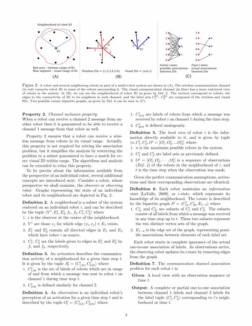
Figure 2: A robot and several neighboring robots as part of a multi-robot system are shown in (A). The wireless communication channel(in red) connects robot R1 to some of the robots surrounding it. The visual communication channel (in blue) has a more restricted viewof robots in the system. In (B), we can see the neighborhood of robot R1 as given by Def. 2. The vertices correspond to robots, theedges to the connectivity of R1 to its neighbors in each channel, and the label sets CR1

1 , CR12 are composed of the wireless and visual

IDs. Two possible i-state bipartite graphs, as given by Def. 6 can be seen in (C).

Property 2. Channel inclusion property:When a robot can receive a channel 2 message from an-other robot then it is guaranteed to be able to receive achannel 1 message from that robot as well.

Property 2 ensures that a robot can receive a wire-less message from robots in its visual range. Actually,this property is not required for solving the associationproblem, but it simplifies the analysis by restricting theproblem to a subset guaranteed to have a match for ev-ery visual ID within range. The algorithms and analysiscan be extended to relax this property.

To be precise about the information available fromthe perspective of an individual robot, several additionalconcepts are introduced next. Consider a robot, whoseperspective we shall examine, the observer or observingrobot. Graphs representing the state of an individualrobot and its neighborhood are depicted in Fig. 2.

Definition 2. A neighborhood is a subset of the systemcentered on an individual robot i, and can be describedby the tuple 〈V i, Ei

1, Ei2, f1, f2, C

i1, C

i2〉 where

1. i is the observer at the center of the neighborhood.

2. V i are those vj for which edge (vi, vj) ∈ E1 exists.

3. Ei1 and Ei

2 contain all directed edges in E1 and E2

which have robot i as source.

4. Ci1, Ci

2 are the labels given to edges in Ei1 and Ei

2 byf1 and f2, respectively.

Definition 3. An activation describes the communica-tion activity of a neighborhood for a given time step t.It is given by the tuple Ai

t = 〈Ci1At, C

i2At〉 where

1. Ci1At is the set of labels of robots which are in range

of and from which a message was sent to robot i onchannel 1 during time step t.

2. Ci2At is defined similarly for channel 2.

Definition 4. An observation is an individual robot’sperception of an activation for a given time step t and isdescribed by the tuple Oi

t = 〈Ci1Ot, C

i2Ot〉 where

1. Ci1Ot are labels of robots from which a message was

received by robot i on channel 1 during the time step.

2. Ci2Ot is defined analogously.

Definition 5. The local view of robot i is the infor-mation directly available to it, and is given by tuple〈n,Ci

1, Ci2, O

i = [Oi1, O

i2, ...O

it]〉 where

1. n is the maximum possible robots in the system.

2. Ci1 and Ci

2 are label sets as previously defined.

3. Oi = [Oi1, O

i2, · · · , Oi

t] is a sequence of observations(Def. 4) of the robots in the neighborhood of i, andt is the time step when the observation was made.

Given the perfect communication assumptions, activa-tions and their corresponding observations are identical.

Definition 6. Each robot maintains an informationstate [LaValle, 2009], or i-state, which represents itsknowledge of its neighborhood. The i-state is describedby the bipartite graph Si = 〈Ci

1t, Ci2t, E1−2〉 where

1. Ci1t and Ci

2t are subsets of Ci1 and Ci

2. The subsetsconsist of all labels from which a message was receivedin any time step up to t. These two subsets representthe two distinct vertex sets of the graph.

2. E1−2 is the edge set of the graph, representing possi-ble associations between elements of each label set.

Each robot starts in complete ignorance of the actualone-to-one association of labels. As observations arrive,the observing robot updates its i-state by removing edgesfrom the graph.

Definition 7. The communication channel associationproblem for each robot i is:

Given: A local view with an observation sequence attime t.

Output: A complete or partial one-to-one associationbetween channel 1 labels and channel 2 labels forthe label tuple 〈Ci

1, Ci2〉 corresponding to i’s neigh-

borhood at time t.

4

111111111111

2

100011011011

101010101101

110110001001

110110001110

101010101010

100011011100

111111111000

4

100011011000

100010001001

100010001010

4

101010101000

100010001100

4

110110001000

100010001000

4 4 44

8 888 8 8

16

8 88 8 8 8

44

44

4

44

4

44

4

44

4

44

4

44

4

4

22

2

2 2 2

2

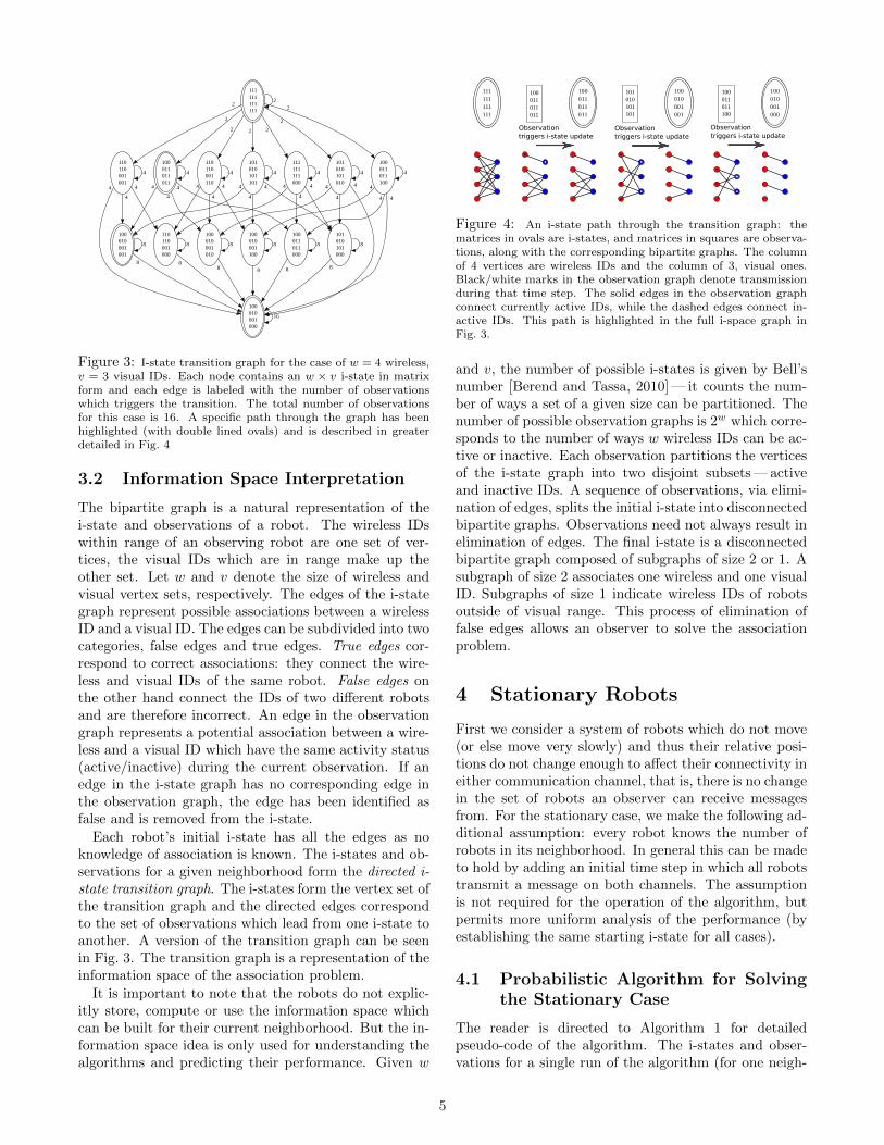
Figure 3: I-state transition graph for the case of w = 4 wireless,v = 3 visual IDs. Each node contains an w × v i-state in matrixform and each edge is labeled with the number of observationswhich triggers the transition. The total number of observationsfor this case is 16. A specific path through the graph has beenhighlighted (with double lined ovals) and is described in greaterdetailed in Fig. 4

3.2 Information Space Interpretation

The bipartite graph is a natural representation of thei-state and observations of a robot. The wireless IDswithin range of an observing robot are one set of ver-tices, the visual IDs which are in range make up theother set. Let w and v denote the size of wireless andvisual vertex sets, respectively. The edges of the i-stategraph represent possible associations between a wirelessID and a visual ID. The edges can be subdivided into twocategories, false edges and true edges. True edges cor-respond to correct associations: they connect the wire-less and visual IDs of the same robot. False edges onthe other hand connect the IDs of two different robotsand are therefore incorrect. An edge in the observationgraph represents a potential association between a wire-less and a visual ID which have the same activity status(active/inactive) during the current observation. If anedge in the i-state graph has no corresponding edge inthe observation graph, the edge has been identified asfalse and is removed from the i-state.

Each robot’s initial i-state has all the edges as noknowledge of association is known. The i-states and ob-servations for a given neighborhood form the directed i-state transition graph. The i-states form the vertex set ofthe transition graph and the directed edges correspondto the set of observations which lead from one i-state toanother. A version of the transition graph can be seenin Fig. 3. The transition graph is a representation of theinformation space of the association problem.

It is important to note that the robots do not explic-itly store, compute or use the information space whichcan be built for their current neighborhood. But the in-formation space idea is only used for understanding thealgorithms and predicting their performance. Given w

111111111111

100011011011

100010001001

100010001000

100011011100

100011011011

101010101101

Observation triggers i-state update



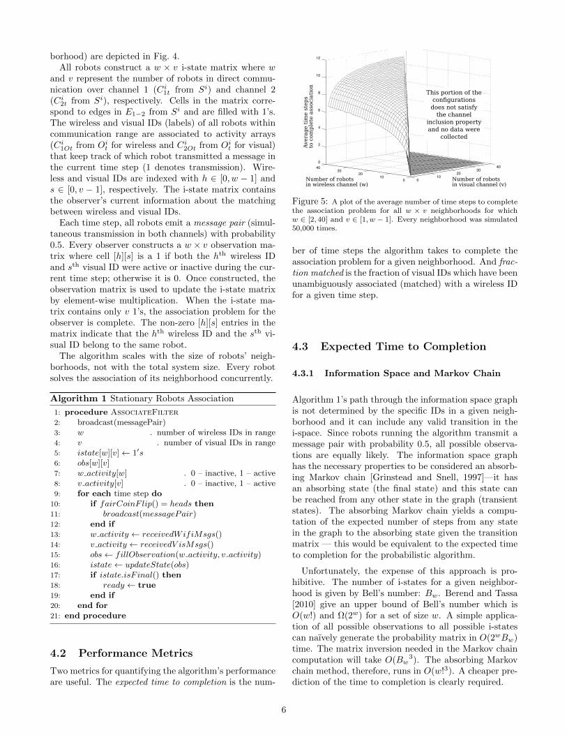
Figure 4: An i-state path through the transition graph: thematrices in ovals are i-states, and matrices in squares are observa-tions, along with the corresponding bipartite graphs. The columnof 4 vertices are wireless IDs and the column of 3, visual ones.Black/white marks in the observation graph denote transmissionduring that time step. The solid edges in the observation graphconnect currently active IDs, while the dashed edges connect in-active IDs. This path is highlighted in the full i-space graph inFig. 3.

and v, the number of possible i-states is given by Bell’snumber [Berend and Tassa, 2010] — it counts the num-ber of ways a set of a given size can be partitioned. Thenumber of possible observation graphs is 2w which corre-sponds to the number of ways w wireless IDs can be ac-tive or inactive. Each observation partitions the verticesof the i-state graph into two disjoint subsets — activeand inactive IDs. A sequence of observations, via elimi-nation of edges, splits the initial i-state into disconnectedbipartite graphs. Observations need not always result inelimination of edges. The final i-state is a disconnectedbipartite graph composed of subgraphs of size 2 or 1. Asubgraph of size 2 associates one wireless and one visualID. Subgraphs of size 1 indicate wireless IDs of robotsoutside of visual range. This process of elimination offalse edges allows an observer to solve the associationproblem.

4 Stationary Robots

First we consider a system of robots which do not move(or else move very slowly) and thus their relative posi-tions do not change enough to affect their connectivity ineither communication channel, that is, there is no changein the set of robots an observer can receive messagesfrom. For the stationary case, we make the following ad-ditional assumption: every robot knows the number ofrobots in its neighborhood. In general this can be madeto hold by adding an initial time step in which all robotstransmit a message on both channels. The assumptionis not required for the operation of the algorithm, butpermits more uniform analysis of the performance (byestablishing the same starting i-state for all cases).

4.1 Probabilistic Algorithm for Solvingthe Stationary Case

The reader is directed to Algorithm 1 for detailedpseudo-code of the algorithm. The i-states and obser-vations for a single run of the algorithm (for one neigh-

5

borhood) are depicted in Fig. 4.All robots construct a w × v i-state matrix where w

and v represent the number of robots in direct commu-nication over channel 1 (Ci

1t from Si) and channel 2(Ci

2t from Si), respectively. Cells in the matrix corre-spond to edges in E1−2 from Si and are filled with 1’s.The wireless and visual IDs (labels) of all robots withincommunication range are associated to activity arrays(Ci

1Ot from Oit for wireless and Ci

2Ot from Oit for visual)

that keep track of which robot transmitted a message inthe current time step (1 denotes transmission). Wire-less and visual IDs are indexed with h ∈ [0, w − 1] ands ∈ [0, v − 1], respectively. The i-state matrix containsthe observer’s current information about the matchingbetween wireless and visual IDs.

Each time step, all robots emit a message pair (simul-taneous transmission in both channels) with probability0.5. Every observer constructs a w × v observation ma-trix where cell [h][s] is a 1 if both the hth wireless IDand sth visual ID were active or inactive during the cur-rent time step; otherwise it is 0. Once constructed, theobservation matrix is used to update the i-state matrixby element-wise multiplication. When the i-state ma-trix contains only v 1’s, the association problem for theobserver is complete. The non-zero [h][s] entries in thematrix indicate that the hth wireless ID and the sth vi-sual ID belong to the same robot.

The algorithm scales with the size of robots’ neigh-borhoods, not with the total system size. Every robotsolves the association of its neighborhood concurrently.

Algorithm 1 Stationary Robots Association

1: procedure AssociateFilter2: broadcast(messagePair)3: w . number of wireless IDs in range4: v . number of visual IDs in range5: istate[w][v]← 1′s6: obs[w][v]7: w activity[w] . 0 – inactive, 1 – active8: v activity[v] . 0 – inactive, 1 – active9: for each time step do

10: if fairCoinF lip() = heads then11: broadcast(messagePair)12: end if13: w activity ← receivedWifiMsgs()14: v activity ← receivedV isMsgs()15: obs← fillObservation(w activity, v activity)16: istate← updateState(obs)17: if istate.isF inal() then18: ready ← true19: end if20: end for21: end procedure

4.2 Performance Metrics

Two metrics for quantifying the algorithm’s performanceare useful. The expected time to completion is the num-

0

2

4

6

8

10

1020

3040

12

0 010

2030

40

This portion of the configurations does not satisfy

the channel inclusion property and no data were

collected

Number of robotsin wireless channel (w)

Ave

rag

eti

me

step

sto

com

ple

teass

oci

ati

on

Number of robotsin visual channel (v)

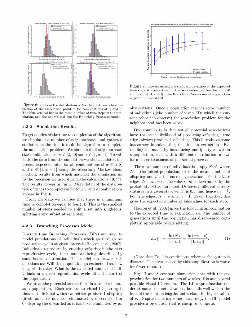
Figure 5: A plot of the average number of time steps to completethe association problem for all w × v neighborhoods for whichw ∈ [2, 40] and v ∈ [1, w − 1]. Every neighborhood was simulated50,000 times.

ber of time steps the algorithm takes to complete theassociation problem for a given neighborhood. And frac-tion matched is the fraction of visual IDs which have beenunambiguously associated (matched) with a wireless IDfor a given time step.

4.3 Expected Time to Completion

4.3.1 Information Space and Markov Chain

Algorithm 1’s path through the information space graphis not determined by the specific IDs in a given neigh-borhood and it can include any valid transition in thei-space. Since robots running the algorithm transmit amessage pair with probability 0.5, all possible observa-tions are equally likely. The information space graphhas the necessary properties to be considered an absorb-ing Markov chain [Grinstead and Snell, 1997]—it hasan absorbing state (the final state) and this state canbe reached from any other state in the graph (transientstates). The absorbing Markov chain yields a compu-tation of the expected number of steps from any statein the graph to the absorbing state given the transitionmatrix — this would be equivalent to the expected timeto completion for the probabilistic algorithm.

Unfortunately, the expense of this approach is pro-hibitive. The number of i-states for a given neighbor-hood is given by Bell’s number: Bw. Berend and Tassa[2010] give an upper bound of Bell’s number which isO(w!) and Ω(2w) for a set of size w. A simple applica-tion of all possible observations to all possible i-statescan naıvely generate the probability matrix in O(2wBw)time. The matrix inversion needed in the Markov chaincomputation will take O(Bw

3). The absorbing Markovchain method, therefore, runs in O(w!3). A cheaper pre-diction of the time to completion is clearly required.

6

1 2 3 4 5 6 7 8 9 10 11 12 13 14 15 16 17 18 19 200

0.05

0.1

0.15

0.2

0.25

0.3

0.35

Time steps taken to associate all visual IDs

Frac

tion

of tr

ials

com

plet

ed b

y a

give

n tim

e st

ep

Number of wireless IDs = 40 | Number of visual IDs = 39

Trial distribution

Simulation mean: 10.944 ts

BP model prediction: 10.571 ts

1 2 3 4 5 6 7 8 9 10 11 12 13 14 15 16 17 18 19 200

0.05

0.1

0.15

0.2

0.25

0.3

0.35


Frac

tion

of tr

ials

com

plet

ed b

y a

give

n tim

e st

ep


Trial distribution



1 2 3 4 5 6 7 8 9 10 11 12 13 14 15 16 17 18 19 200

0.05

0.1

0.15

0.2

0.25

0.3

0.35


Frac

tion

of tr

ials

com

plet

ed b

y a

give

n tim

e st

ep


Trial distribution



1 2 3 4 5 6 7 8 9 10 11 12 13 14 15 16 17 18 19 200

0.05

0.1

0.15

0.2

0.25

0.3

0.35


Frac

tion

of tr

ials

com

plet

ed b

y a

give

n tim

e st

ep


Trial distribution



Figure 6: Plots of the distribution of the different times to com-pletion of the association problem for combinations of w and v.The blue vertical line is the mean number of time steps in the sim-ulation, and the red vertical line the Branching Processes model.

4.3.2 Simulation Results

To get an idea of the time to completion of the algorithm,we simulated a number of neighborhoods and gatheredstatistics on the time it took the algorithm to completethe association problem. We simulated all neighborhoodsize combinations of w ∈ [2, 40] and v ∈ [1, w−1]. To val-idate the data from the simulation we also calculated theprecise expected value for all combinations of w ∈ [2, 8]and v ∈ [1, w − 1] using the absorbing Markov chainmethod, results from which matched the simulation upto the precision we used during the calculations (10−4).The results appear in Fig. 5. More detail of the distribu-tion of times to completion for four w and v combinationsappear in Fig. 6.

From the data we can see that there is a minimumtime to completion equal to log2(v). This is the smallestnumber of steps needed to split a set into singletons,splitting every subset at each step.

4.3.3 Branching Processes Model

Discrete time Branching Processes (BPs) are used tomodel populations of individuals which go through re-productive cycles at given intervals [Haccou et al., 2007].Individuals reproduce by creating offspring in the nextreproductive cycle, their number being described bysome known distribution. The model can answer suchquestions as: Will this population go extinct? If so, howlong will it take? What is the expected number of indi-viduals in a given reproduction cycle after the start ofthe population?

We treat the potential associations in a robot’s i-stateas a population. Each wireless to visual ID pairing isthus an individual which can either produce 1 offspring(itself, as it has not been eliminated by observation) or0 offspring (be discarded as it has been eliminated by an

0 5 10 15 202

4

6

8

10

12

Number of visual IDs in communication range

Ave

rage

tim

e st

eps

to a

ssoc

iate

all

visu

al ID

s

Comparison between simulation data and BP model for 20 wireless IDs

Simulation data

BP model prediction

Figure 7: The mean and one standard deviation of the expectedtime steps to completion for the association problem for w = 20and odd v ∈ [1, w− 1]. The Branching Process model’s predictionis given in dashed red.

observation). Once a population reaches some numberof individuals (the number of visual IDs which the cur-rent robot can observe) the association problem for theneighborhood has been solved.

One complexity is that not all potential associationshave the same likelihood of producing offspring—trueedges always produce 1 offspring. This introduces someinaccuracy in calculating the time to extinction. Ex-tending the model by introducing multiple types withina population, each with a different distribution, allowsfor a closer treatment of the actual process.

The mean number of individuals is simply Nmt, whereN is the initial population, m is the mean number ofoffspring and t is the current generation. For the falseedges, N = wv−v. The value of m is determined by theprobability of two unrelated IDs having different activitystatuses in a given step, which is 0.5, and hence m = 1

2 .For true edges, N = v and m = 1. Taken together, thisgives the expected number of false edges for each step.

Haccou et al. [2007] gives the following approximationto the expected time to extinction, i.e., the number ofgenerations until the population has disappeared com-pletely, applicable to our setting:

EN [τ ] =ln (N)

| ln (m)|=

ln (wv − v)

| ln (12 )|

. (1)

(Note that Eq. 1 is continuous, whereas the system isdiscrete. The error caused by this simplification is worsefor fewer robots.)

Figs. 7 and 8 compare simulation data with the ap-proximation for two numbers of wireless IDs and severalpossible visual ID counts. The BP approximation un-derestimates the actual values, but falls well within thebulk of the solution lengths and is closer for higher valuesof v. Despite incurring some inaccuracy, the BP modelprovides a prediction that is cheap to compute.

7

0 10 20 30 404

6

8

10

12

14

Number of visual IDs in communication range

Ave

rage

tim

e st

eps

to a

ssoc

iate

all

visu

al ID

s

Comparison between simulation data and BP model for 40 wireless IDs

Simulation data

BP model prediction

Figure 8: Data as in Fig. 7 but for w = 40.

4.4 Fraction Matched Metric

4.4.1 Simulation Results

Keeping the simulation setup as before, an average ofthe fraction matched metric over several simulation runs,for neighborhoods of different sizes, was computed andappears in Fig. 9. In addition, to the time to completion,we kept track of the number of visual IDs unambiguouslyassociated with a wireless ID. From this we computed theexpected fraction of visual IDs solved at each time step.

4.4.2 Fraction Matched Model

To predict fraction matched we set w = v since empiricalobservations showed that, under our assumptions, thereis no dependence on v. The starting number of falseedges is wv − v and, thereafter, one can compute theexpected number of false edges via Eq.(2) to give a valuefor each time step.

Ft = Finit ×mt. (2)

Next, for every visual ID, we calculate the probabilitythat it will have zero false edges assigned to it, as thisrepresents an unambiguously associated visual ID. Thevalue is equal to the probability that all false edges havebeen assigned to any of the rest of the visual IDs, whichis given by Eq. (3). The same equation also producesthe fraction of unambiguously associated visual IDs.

Pmatched =

(v − 1

v

)Ft

. (3)

The following simplifications have been introduced toboiling this probabilistic, combinatorial problem in sucha concise characterization. First, we assume each visualID is independent from the other visual IDs. Second,when looking from the perspective of a single visual ID,that there is no limit on how many false edges may beassigned to the other visual IDs. A comparison betweenthe model’s prediction and simulation results can be seenin Fig. 9. This simple model is startlingly effective.

0 2 4 6 8 100

0.2

0.4

0.6

0.8

1

Time steps since the algorithm started

Frac

tion

of v

isua

l ID

s as

soci

ated

with

a w

irele

ss ID

Simulation results for fraction matched metric

W = 2W = 4

W = 8W = 16

W = 30W = 60

W = 100

Simulation data

Model prediction

Figure 9: Predictions of the model compared with simulationperformance for the fraction matched metric across different num-bers of wireless IDs (w).

5 Moving Robots

Next, we examine the channel association problem inwhich a subset of the robots move fast enough to causeconnectivity changes during the execution.

5.1 Information Space and States

In the mobile case, the associated i-state and i-spacestructures and their respective sizes may change as therobots move. We assume that this change may occurevery time step of the algorithm, thus, the associationproblem can be imagined as a two part process. Onesubprocess acts multiplicatively to reduce the number offalse edges as in the stationary robot case. But now asecond subprocess acts additively, introducing new edgesto the process. Eq. 4 models these two processes:

Tt = (Tt−1 ×m) +Nt. (4)

Here Tt is the total number of edges for time step t,Tt−1 denotes the number of edges in the previous step,and Nt is the number of newly added edges, with m, amultiplicative factor m < 1, giving the dependence ofedges from one time step to the next.

5.2 Algorithm for Mobile Robots

The algorithm in Section 4.1 needs some modification tohandle the dynamic nature of the moving robot’s neigh-borhood. The evolving information state must distin-guish between new and old IDs, and old IDs which areno longer in range should be removed. Unlike the sta-tionary case, we do not assume that the full number ofrobots (IDs) which are in range is known in advance.

A new wireless ID enters an observer’s range as soonas a message is received from it, which can only happenwhen the ID is both in range and active. Visual IDs,on the other hand, can enter the range of an observerbefore they activate since the robot can distinguish a

8

neighbor even when it is not transmitting through thevisual channel. But since adding a visual ID before itis activated brings no practical information, we may ig-nore visual IDs which are inactive and only add themto the observer’s i-state once they activate. This, givenour earlier assumptions, guarantees that there will be atleast one candidate wireless ID to be associated with thevisual ID.

Visual IDs can simply be removed when they leave therobot’s range. This does not apply to wireless IDs sincean observing robot cannot detect when a robot has leftits wireless range. Thus, the observer needs to keep trackof how long a wireless ID has been inactive. If, after apre-set number of time steps, an ID has been inactive,it is dropped from the list. By choosing an appropriatedrop time, the robot limits the number of IDs it tracksand also guards against losing too much information bydropping IDs too soon.

We note that it is possible for the algorithm to operatewithout dropping wireless IDs, but this runs the risk ofcreating unnecessary work with little or no benefit. Forexample, if a robot is likely to see most of the IDs in thesystem, but will only be in communication range withrelatively few, then there is no need to keep old wirelessIDs around. Since the algorithm only adds potentialedges between active IDs, a wireless ID which has beenencountered before but subsequently dropped, will beadded back as soon as it is detected. Furthermore, visualIDs are dynamically assigned to the robots in range bythe observing robot. This means that a wireless ID whichre-enters communication range is unlikely to be matchedwith the same visual ID, making keeping the old wirelessID around even less useful.

A major change to Algorithm 1 is a procedure whichmodifies the i-state based on the list of new and re-moved IDs before it updates the i-state using the currenttime step’s observation. The procedure removes rowsand columns from the i-state corresponding to wirelessand visual IDs which have exited their respective ranges.The procedure also adds new rows and columns into thei-state for new wireless and visual IDs. Once new IDshave been added, the appropriate edges between verticesneed to be added to the i-state as well. Edges are addedas follows. An edge is added between all new wirelessand new visual IDs. In the case of equal wireless andvisual range, no more edges are added. In the case ofthe wireless range being greater than the visual range,new edges are added between all new visual IDs and old,not yet associated, active wireless IDs. This is necessarybecause a robot can enter wireless communication rangemuch sooner than it will enter the visual communicationrange of an observer. This means that a newly added vi-sual ID may be matched with a wireless ID which has al-ready been included in the i-state of the observing robot.In this work, we only examine the case where the wire-less range is equal to the visual range. The pseudo-codefor the mobile version of algorithm can be seen in Algo-

rithm 2.

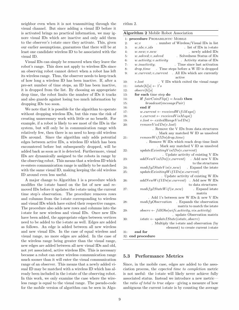
Algorithm 2 Mobile Robot Association

1: procedure Probabilistic Mobile2: w; v . number of Wireless/Visual IDs in list3: w ids; v ids . list of IDs in i-state4: w new; v new . newly added IDs5: w solved; v solved . Solvedness Status of IDs6: w activity; v activity . Activity status of IDs7: w inactivity; . Time since last activation8: drop time . Time steps before a W ID is dropped9: w current; v current . All IDs which are currently

. active10: v lost . V IDs which exited the visual range11: istate[h][s]← 1′s12: observ[h][s]13: for each time step do14: if fairCoinF lip() = heads then15: broadcast(messagePair)16: end if17: w current← receivedWifiMsgs()18: v current← receivedV isMsgs()19: v lost← exitedRangeV isIDs()20: removeV isIDs(v lost)

. . Remove the V IDs from data structures

. . Mark any matched W ID as unsolved21: removeWifIDs(drop time)

. . Remove W IDs which reach drop time limit

. . Mark any matched V ID as unsolved22: updateExisitingV isIDs(v current)

. . Update activity of existing V IDs23: addNewV isIDs((v current) . Add new V IDs

. to the structures24: modifyIStateV is(v new) . Expand the istate25: updateExisitingWifIDs(w current)

. . Update activity of existing W IDs26: addNewWifIDs(w current) . Add new W IDs

. to data structures27: modifyIStateWif(w new) . Expand istate

. matrix

. . Add 1’s between new W IDs & new V IDs28: modifyObservation . Expands the observation

. matrix to match the istate29: observ ← fillObs(wifi activity, vis activity)

. . update Observation matrix30: istate← updateIState(istate, observ)

. . Multiply the i-state and observation (by

. element) to create current i-state31: end for32: end procedure

5.3 Performance Metrics

Since, in the mobile case, edges are added to the asso-ciation process, the expected time to completion metricis not useful: the i-state will likely never achieve fullyassociated status. Instead we introduce a new metric—the ratio of total to true edges—giving a measure of howambiguous the current i-state is by counting the average

9

0 10 20 30 400.2

0.4

0.6

0.8

1

Time since beginning of algorithm

Frac

tion

visu

al ID

s m

atch

ed

Fraction matched for 3 different population mixes

10% mobile robots

50% mobile robots

90% mobile robots

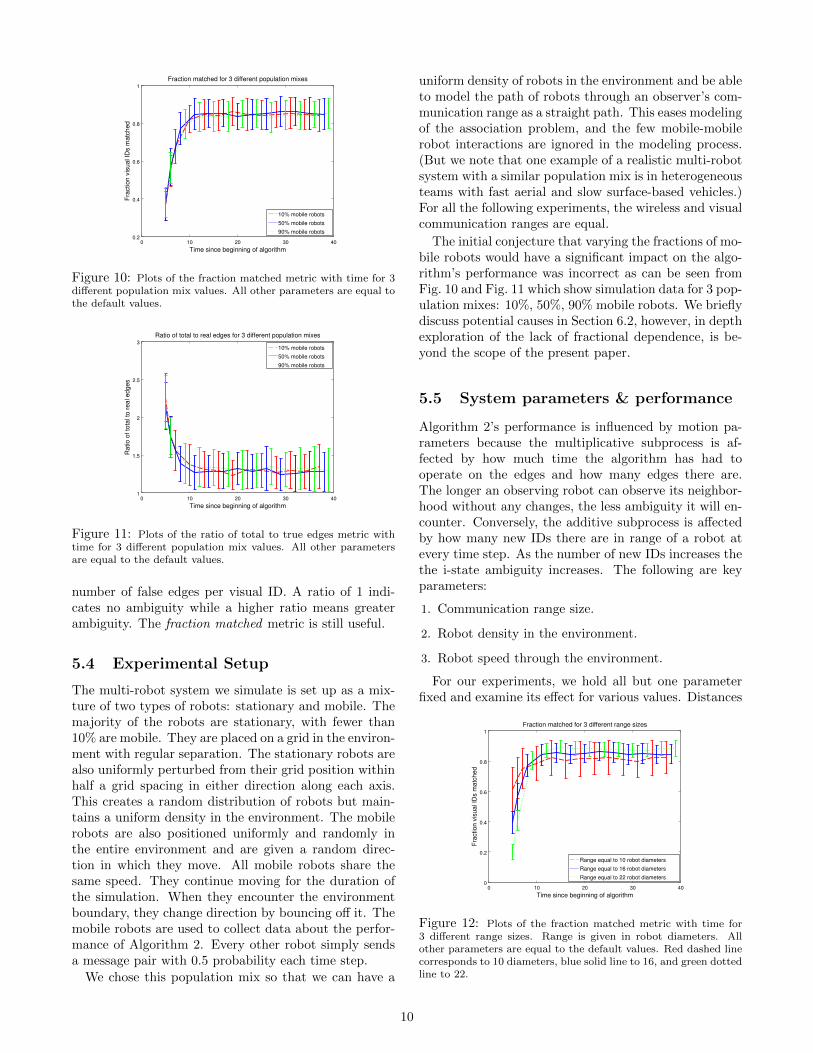
Figure 10: Plots of the fraction matched metric with time for 3different population mix values. All other parameters are equal tothe default values.

0 10 20 30 401

1.5

2

2.5

3


Rat

io o

f tot

al to

real

edg

es

Ratio of total to real edges for 3 different population mixes

10% mobile robots

50% mobile robots

90% mobile robots

Figure 11: Plots of the ratio of total to true edges metric withtime for 3 different population mix values. All other parametersare equal to the default values.

number of false edges per visual ID. A ratio of 1 indi-cates no ambiguity while a higher ratio means greaterambiguity. The fraction matched metric is still useful.

5.4 Experimental Setup

The multi-robot system we simulate is set up as a mix-ture of two types of robots: stationary and mobile. Themajority of the robots are stationary, with fewer than10% are mobile. They are placed on a grid in the environ-ment with regular separation. The stationary robots arealso uniformly perturbed from their grid position withinhalf a grid spacing in either direction along each axis.This creates a random distribution of robots but main-tains a uniform density in the environment. The mobilerobots are also positioned uniformly and randomly inthe entire environment and are given a random direc-tion in which they move. All mobile robots share thesame speed. They continue moving for the duration ofthe simulation. When they encounter the environmentboundary, they change direction by bouncing off it. Themobile robots are used to collect data about the perfor-mance of Algorithm 2. Every other robot simply sendsa message pair with 0.5 probability each time step.

We chose this population mix so that we can have a

uniform density of robots in the environment and be ableto model the path of robots through an observer’s com-munication range as a straight path. This eases modelingof the association problem, and the few mobile-mobilerobot interactions are ignored in the modeling process.(But we note that one example of a realistic multi-robotsystem with a similar population mix is in heterogeneousteams with fast aerial and slow surface-based vehicles.)For all the following experiments, the wireless and visualcommunication ranges are equal.

The initial conjecture that varying the fractions of mo-bile robots would have a significant impact on the algo-rithm’s performance was incorrect as can be seen fromFig. 10 and Fig. 11 which show simulation data for 3 pop-ulation mixes: 10%, 50%, 90% mobile robots. We brieflydiscuss potential causes in Section 6.2, however, in depthexploration of the lack of fractional dependence, is be-yond the scope of the present paper.

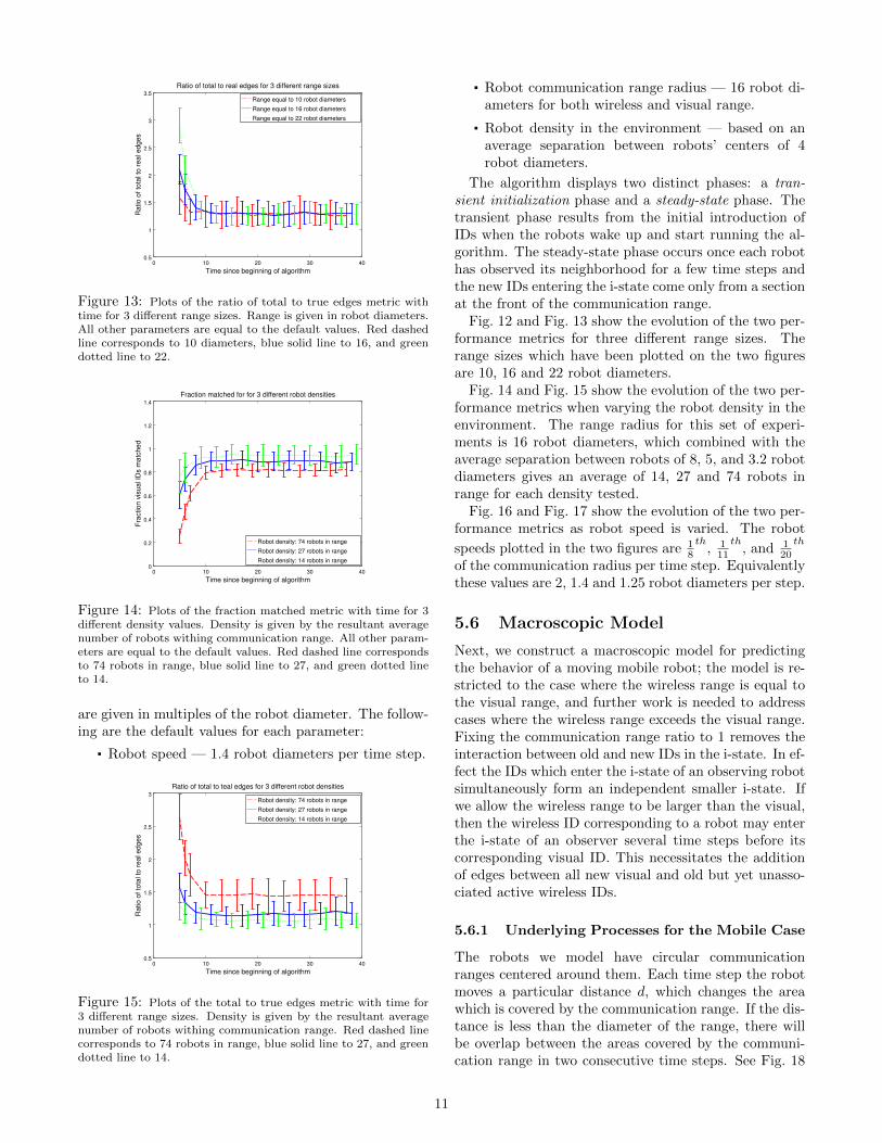
5.5 System parameters & performance

Algorithm 2’s performance is influenced by motion pa-rameters because the multiplicative subprocess is af-fected by how much time the algorithm has had tooperate on the edges and how many edges there are.The longer an observing robot can observe its neighbor-hood without any changes, the less ambiguity it will en-counter. Conversely, the additive subprocess is affectedby how many new IDs there are in range of a robot atevery time step. As the number of new IDs increases thethe i-state ambiguity increases. The following are keyparameters:

1. Communication range size.

2. Robot density in the environment.

3. Robot speed through the environment.

For our experiments, we hold all but one parameterfixed and examine its effect for various values. Distances

0 10 20 30 400

0.2

0.4

0.6

0.8

1


Frac

tion

visu

al ID

s m

atch

ed

Fraction matched for 3 different range sizes

Range equal to 10 robot diameters



Figure 12: Plots of the fraction matched metric with time for3 different range sizes. Range is given in robot diameters. Allother parameters are equal to the default values. Red dashed linecorresponds to 10 diameters, blue solid line to 16, and green dottedline to 22.

10

0 10 20 30 400.5

1

1.5

2

2.5

3

3.5


Rat

io o

f tot

al to

real

edg

es

Ratio of total to real edges for 3 different range sizes




Figure 13: Plots of the ratio of total to true edges metric withtime for 3 different range sizes. Range is given in robot diameters.All other parameters are equal to the default values. Red dashedline corresponds to 10 diameters, blue solid line to 16, and greendotted line to 22.

0 10 20 30 400

0.2

0.4

0.6

0.8

1

1.2

1.4


Frac

tion

visu

al ID

s m

atch

ed

Fraction matched for for 3 different robot densities

Robot density: 74 robots in range



Figure 14: Plots of the fraction matched metric with time for 3different density values. Density is given by the resultant averagenumber of robots withing communication range. All other param-eters are equal to the default values. Red dashed line correspondsto 74 robots in range, blue solid line to 27, and green dotted lineto 14.

are given in multiples of the robot diameter. The follow-ing are the default values for each parameter:

Robot speed — 1.4 robot diameters per time step.

0 10 20 30 400.5

1

1.5

2

2.5

3


Rat

io o

f tot

al to

real

edg

es

Ratio of total to teal edges for 3 different robot densities




Figure 15: Plots of the total to true edges metric with time for3 different range sizes. Density is given by the resultant averagenumber of robots withing communication range. Red dashed linecorresponds to 74 robots in range, blue solid line to 27, and greendotted line to 14.

Robot communication range radius — 16 robot di-ameters for both wireless and visual range.

Robot density in the environment — based on anaverage separation between robots’ centers of 4robot diameters.

The algorithm displays two distinct phases: a tran-sient initialization phase and a steady-state phase. Thetransient phase results from the initial introduction ofIDs when the robots wake up and start running the al-gorithm. The steady-state phase occurs once each robothas observed its neighborhood for a few time steps andthe new IDs entering the i-state come only from a sectionat the front of the communication range.

Fig. 12 and Fig. 13 show the evolution of the two per-formance metrics for three different range sizes. Therange sizes which have been plotted on the two figuresare 10, 16 and 22 robot diameters.

Fig. 14 and Fig. 15 show the evolution of the two per-formance metrics when varying the robot density in theenvironment. The range radius for this set of experi-ments is 16 robot diameters, which combined with theaverage separation between robots of 8, 5, and 3.2 robotdiameters gives an average of 14, 27 and 74 robots inrange for each density tested.

Fig. 16 and Fig. 17 show the evolution of the two per-formance metrics as robot speed is varied. The robot

speeds plotted in the two figures are 18

th, 1

11

th, and 1

20

th

of the communication radius per time step. Equivalentlythese values are 2, 1.4 and 1.25 robot diameters per step.

5.6 Macroscopic Model

Next, we construct a macroscopic model for predictingthe behavior of a moving mobile robot; the model is re-stricted to the case where the wireless range is equal tothe visual range, and further work is needed to addresscases where the wireless range exceeds the visual range.Fixing the communication range ratio to 1 removes theinteraction between old and new IDs in the i-state. In ef-fect the IDs which enter the i-state of an observing robotsimultaneously form an independent smaller i-state. Ifwe allow the wireless range to be larger than the visual,then the wireless ID corresponding to a robot may enterthe i-state of an observer several time steps before itscorresponding visual ID. This necessitates the additionof edges between all new visual and old but yet unasso-ciated active wireless IDs.

5.6.1 Underlying Processes for the Mobile Case

The robots we model have circular communicationranges centered around them. Each time step the robotmoves a particular distance d, which changes the areawhich is covered by the communication range. If the dis-tance is less than the diameter of the range, there willbe overlap between the areas covered by the communi-cation range in two consecutive time steps. See Fig. 18

11

0 10 20 30 400.2

0.4

0.6

0.8

1


Frac

tion

visu

al ID

s m

atch

ed

Fraction matched for 3 different robot speeds

Robot speed 1/20th of range



Figure 16: Changes in the fraction matched metric with timefor 3 different robot speeds. Robot speed is given in fractions ofthe communication range radius. All other parameters are equalto the default values. Red dashed line corresponds to 1/20th ofrange, blue solid lines to 1/11th, and green dotted lines to 1/8th.

0 10 20 30 400.5

1

1.5

2

2.5

3


Rat

io o

f tot

al to

real

edg

es

Ratio of total to real edges for 3 different robot speeds




Figure 17: The changes in the total to true edges metric withtime for 3 different robot speeds. Robot speed is given in fractionsof the communication range radius. All other parameters are equalto the default values. Red dashed line corresponds to 1/20th ofrange, blue solid line to 1/11th, and green dotted line to 1/8th.

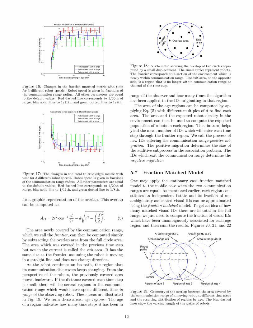
for a graphic representation of the overlap. This overlapcan be computed as:

AO = 2r2 cos−1d

2r− d

√r2 −

(d

2

)2. (5)

The area newly covered by the communication range,which we call the frontier, can then be computed simplyby subtracting the overlap area from the full circle area.The area which was covered in the previous time stepbut not in the current is called the exit area. It has thesame size as the frontier, assuming the robot is movingin a straight line and does not change direction.

As the robot continues on its path, the region thatits communication disk covers keeps changing. From theperspective of the robots, the previously covered areamoves backward. If the distance covered each time stepis small, there will be several regions in the communi-cation range which would have spent different time inrange of the observing robot. These areas are illustratedin Fig. 19. We term these areas, age regions. The ageof a region indicates how many time steps it has been in

Fron

tier

area

Overlap area Exit area

Figure 18: A schematic showing the overlap of two circles sepa-rated by a small displacement. The small circles represent robots.The frontier corresponds to a section of the environment which isnewly within communication range. The exit area, on the oppositeside, is a region that is no longer within communication range atthe end of the time step.

range of the observer and how many times the algorithmhas been applied to the IDs originating in that region.

The area of the age regions can be computed by ap-plying Eq. (5) with different multiples of d to find eacharea. The area and the expected robot density in theenvironment can then be used to compute the expectedpopulation of robots in each region. This, in turn, helpsyield the mean number of IDs which will enter each timestep through the frontier region. We call the process ofnew IDs entering the communication range positive mi-gration. The positive migration determines the size ofthe additive subprocess in the association problem. TheIDs which exit the communication range determine thenegative migration.

5.7 Fraction Matched Model

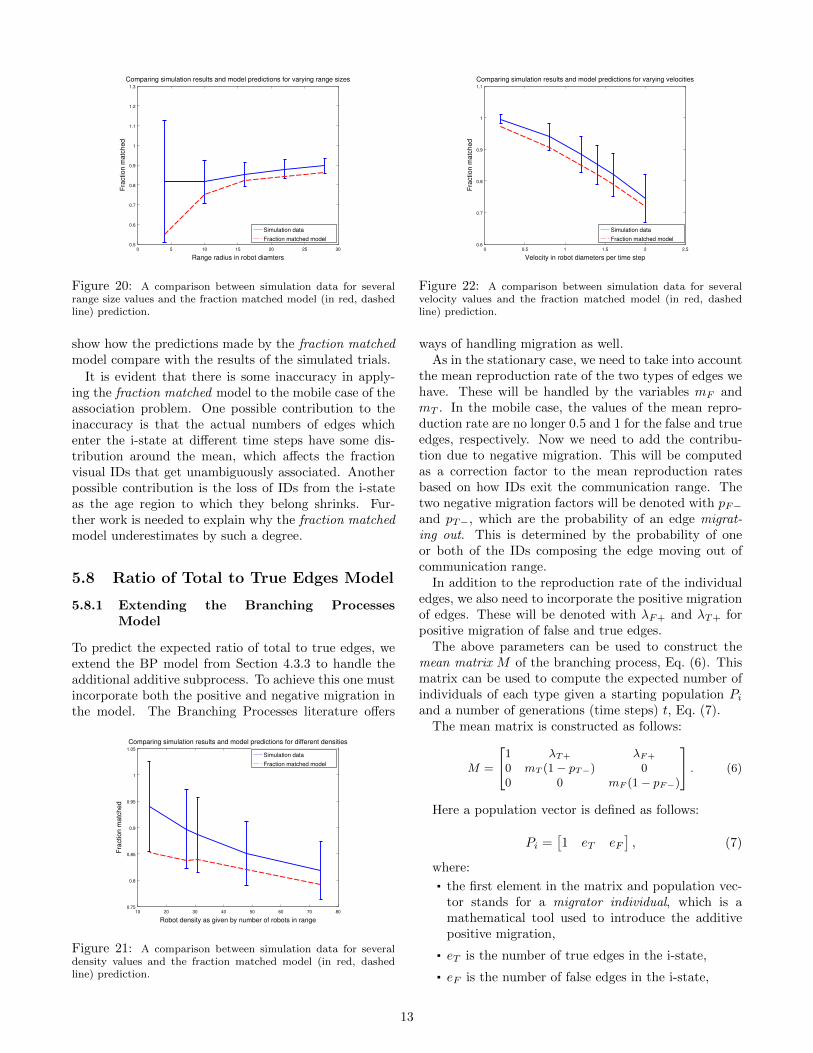
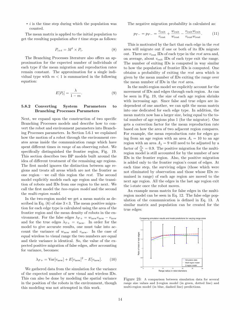
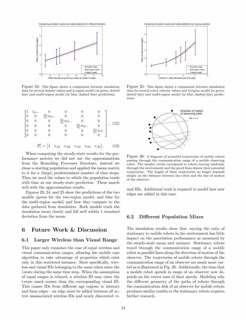
One may apply the stationary case fraction matchedmodel to the mobile case when the two communicationranges are equal. As mentioned earlier, each region con-stitutes an independent i-state and its fraction of un-ambiguously associated visual IDs can be approximatedusing the fraction matched model. To get an idea of howmany matched visual IDs there are in total in the fullrange, we just need to compute the fraction of visual IDswhich have been unambiguously associated for each ageregion and then sum the results. Figures 20, 21, and 22

Area in range at t

Area in range at t-1 Area in range at t-2

Area in range at t-3

Robot paths

Frontier

Region of age 3 Region of age 4Region of age 2

Figure 19: Geometry of the overlap between the area covered bythe communication range of a moving robot at different time stepsand the resulting distribution of regions by age. The blue dashedlines show the varying length of the paths of robots.

12

0 5 10 15 20 25 300.5

0.6

0.7

0.8

0.9

1

1.1

1.2

1.3

Range radius in robot diamters

Frac

tion

mat

ched

Comparing simulation results and model predictions for varying range sizes

Simulation data

Fraction matched model

Figure 20: A comparison between simulation data for severalrange size values and the fraction matched model (in red, dashedline) prediction.

show how the predictions made by the fraction matchedmodel compare with the results of the simulated trials.

It is evident that there is some inaccuracy in apply-ing the fraction matched model to the mobile case of theassociation problem. One possible contribution to theinaccuracy is that the actual numbers of edges whichenter the i-state at different time steps have some dis-tribution around the mean, which affects the fractionvisual IDs that get unambiguously associated. Anotherpossible contribution is the loss of IDs from the i-stateas the age region to which they belong shrinks. Fur-ther work is needed to explain why the fraction matchedmodel underestimates by such a degree.

5.8 Ratio of Total to True Edges Model

5.8.1 Extending the Branching ProcessesModel

To predict the expected ratio of total to true edges, weextend the BP model from Section 4.3.3 to handle theadditional additive subprocess. To achieve this one mustincorporate both the positive and negative migration inthe model. The Branching Processes literature offers

10 20 30 40 50 60 70 800.75

0.8

0.85

0.9

0.95

1

1.05

Robot density as given by number of robots in range

Frac

tion

mat

ched

Comparing simulation results and model predictions for different densities

Simulation data


Figure 21: A comparison between simulation data for severaldensity values and the fraction matched model (in red, dashedline) prediction.

0 0.5 1 1.5 2 2.50.6

0.7

0.8

0.9

1

1.1

Velocity in robot diameters per time step

Frac

tion

mat

ched

Comparing simulation results and model predictions for varying velocities

Simulation data


Figure 22: A comparison between simulation data for severalvelocity values and the fraction matched model (in red, dashedline) prediction.

ways of handling migration as well.As in the stationary case, we need to take into account

the mean reproduction rate of the two types of edges wehave. These will be handled by the variables mF andmT . In the mobile case, the values of the mean repro-duction rate are no longer 0.5 and 1 for the false and trueedges, respectively. Now we need to add the contribu-tion due to negative migration. This will be computedas a correction factor to the mean reproduction ratesbased on how IDs exit the communication range. Thetwo negative migration factors will be denoted with pF−and pT−, which are the probability of an edge migrat-ing out. This is determined by the probability of oneor both of the IDs composing the edge moving out ofcommunication range.

In addition to the reproduction rate of the individualedges, we also need to incorporate the positive migrationof edges. These will be denoted with λF+ and λT+ forpositive migration of false and true edges.

The above parameters can be used to construct themean matrix M of the branching process, Eq. (6). Thismatrix can be used to compute the expected number ofindividuals of each type given a starting population Pi

and a number of generations (time steps) t, Eq. (7).The mean matrix is constructed as follows:

M =

1 λT+ λF+

0 mT (1− pT−) 00 0 mF (1− pF−)

. (6)

Here a population vector is defined as follows:

Pi =[1 eT eF

], (7)

where:

the first element in the matrix and population vec-tor stands for a migrator individual, which is amathematical tool used to introduce the additivepositive migration,

eT is the number of true edges in the i-state,

eF is the number of false edges in the i-state,

13

i is the time step during which the population wascounted.

The mean matrix is applied to the initial population toget the resulting population after t time steps as follows:

Pi+t = M t × Pi. (8)

The Branching Processes literature also offers an ap-proximation for the expected number of individuals ofeach type if the mean migration and reproduction ratesremain constant. The approximation for a single indi-vidual type with m < 1 is summarized in the followingequation:

E[Pt] =λ

1−m. (9)

5.8.2 Converting System Parameters toBranching Processes Parameters

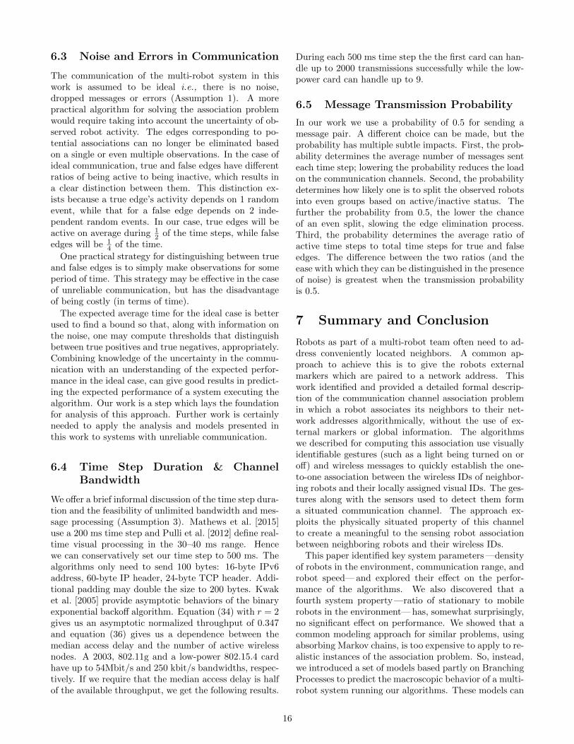
Next, we expand upon the construction of two specificBranching Processes models and describe how to con-vert the robot and environment parameters into Branch-ing Processes parameters. In Section 5.6.1 we explainedhow the motion of a robot through the environment cre-ates areas inside the communication range which havespent different times in range of an observing robot. Wespecifically distinguished the frontier region, Fig. 19.This section describes two BP models built around theidea of different treatment of the remaining age regions.The first model ignores the distinction between age re-gions and treats all areas which are not the frontier asone region — we call this region the rest. The secondmodel explicitly models each age region and the transi-tion of robots and IDs from one region to the next. Wecall the first model the two-region model and the secondthe multi-region model.

In the two-region model we get a mean matrix as de-scribed in Eq. (6) of size 3×3. The mean positive migra-tion for each edge type is calculated using the area of thefrontier region and the mean density of robots in the en-vironment. For the false edges λF+ = wnewvnew − vnewand for the true edges λT+ = vnew. In order for themodel to give accurate results, one must take into ac-count the variance of wnew and vnew. In the case ofequal wireless to visual range the two numbers are equaland their variance is identical. So, the value of the ex-pected positive migration of false edges, after accountingfor variance, becomes:

λF+ = Var[vnew] + E[vnew]2 − E[vnew]. (10)

We gathered data from the simulation for the varianceof the expected number of new visual and wireless IDs.This can also be done by modeling the spatial variancein the position of the robots in the environment, thoughthis modeling was not attempted in this work.

The negative migration probability is calculated as:

pT− = pF− =vexitvrest

+wexit

wrest− vexitwexit

vrestwrest. (11)

This is motivated by the fact that each edge in the restarea will migrate out if one or both of its IDs migrateout. There are vrest IDs of each type in the rest area and,on average, about vexit IDs of each type exit the range.The number of exiting IDs is computed in way similarto how the population of frontier IDs is computed. Oneobtains a probability of exiting the rest area which isgiven by the mean number of IDs exiting the range overthe mean number of IDs in the rest area.

In the multi-region model we explicitly account for themovement of IDs and edges through each region. As canbe seen in Fig. 19, the size of each age region shrinkswith increasing age. Since false and true edges are in-dependent of one another, we can split the mean matrixinto one dedicated for each edge type. In addition, themean matrix now has a larger size, being equal to the to-tal number of age regions plus 1 (for the migrator). Onegets a correction factor for the mean reproduction ratebased on how the area of two adjacent region compares.For example, the mean reproduction rate for edges go-ing from an age region with an area Ai = 10 to an ageregion with an area Aj = 9 will need to be adjusted by a

factor ofAj

Ai= 0.9. The positive migration for the multi-

region model is still accounted for by the number of newIDs in the frontier region. Also, the positive migrationis added only to the frontier region’s count of edges. Ateach time step, the surviving edges (those which werenot eliminated by observation and those whose IDs re-mained in range) of each age region are moved to thenext age region. All the edges in the last age region exitthe i-state once the robot moves.

An example mean matrix for false edges in the multi-region model can be seen in Eq. 12. The false edge pop-ulation of the communication is defined in Eq. 13. Asimilar matrix and population can be created for thetrue edges:

0 5 10 15 20 25 300.6

0.8

1

1.2

1.4

1.6

Range radius in robot diameters

Rat

io o

f tot

al o

f rea

l edg

es

Comparing simulation results and model predictions for varying range sizes

Simulation data

Multi-region model

2-region model

Figure 23: A comparison between simulation data for severalrange size values and 2-region model (in green, dotted line) andmulti-region model (in blue, dashed line) predictions.

14

10 20 30 40 50 60 70 800.8

1

1.2

1.4

1.6

1.8

Robot density as given by number of robots in range

Rat

io o

f tot

al to

real

edg

es

Comparing simulation results and model predictions for different densities

Simulation data

Multi-region model

2-region model

Figure 24: This figure shows a comparison between simulationdata for several density values and 2-region model (in green, dottedline) and multi-region model (in blue, dashed line) predictions.

1 λF+ 0 0 0 0

0 0 A2A1mF− 0 0 0

0 0 0 A3A2mF− 0 0

0 0 0 0 A4A3mF− 0

0 0 0 0 0 A5A4mF−

0 0 0 0 0 0

, (12)

P ′i =[1 eA1 eA2 eA3 eA4 eA5

]. (13)

When computing the steady-state results for the per-formance metrics we did not use the approximationsfrom the Branching Processes literature, instead wechose a starting population and applied the mean matrixto it for a (large) predetermined number of time steps.Then we used the values to which the population tendswith time as our steady-state prediction. These matchwell with the approximation results.

Figures 23, 24, and 25 show the predictions of the twomodels (green for the two-region model, and blue forthe multi-region model) and how they compare to thedata gathered from simulation. Both models track thesimulation mean closely and fall well within 1 standarddeviation from the mean.

6 Future Work & Discussion

6.1 Larger Wireless than Visual Range

This paper only examines the case of equal wireless andvisual communication ranges, allowing the mobile casealgorithm to take advantage of properties which existonly in this restricted instance. More specifically, wire-less and visual IDs belonging to the same robot enter thei-state during the same time step. When the assumptionof equal ranges is relaxed, a wireless ID may enter thei-state much sooner than the corresponding visual ID.This causes IDs from different age regions to interactand form edges—an edge must be added between all ac-tive unassociated wireless IDs and newly discovered vi-

0 0.5 1 1.5 2 2.50.8

1

1.2

1.4

1.6

1.8

2

Velocity in robot diameters per time step

Rat

io o

f tot

al to

real

edg

es

Comparing simulation results and model predictions for varying velocities

Simulation data

Multi-region model

2-region model

Figure 25: This figure shows a comparison between simulationdata for several robot velocity values and 2-region model (in green,dotted line) and multi-region model (in blue, dashed line) predic-tions.

Direction of motion of observing robot

Figure 26: A diagram of potential trajectories of mobile robotspassing through the communication range of a mobile observingrobot. The smaller circles correspond to robots moving randomlythrough the environment and the greed lines denote their potentialtrajectories. The length of these trajectories no longer dependssimply on the distance between the robot and the line of motionof the observer.

sual IDs. Additional work is required to model how newedges are added in this case.

6.2 Different Population Mixes

The simulation results show that varying the ratio ofstationary to mobile robots in the environment has littleimpact on the association performance as measured bythe steady-state mean and variance. Stationary robotstravel through the communication range of a mobilerobot in parallel lines along the direction of motion of theobserver. The trajectories of mobile robots through thecommunication range of an observer are much more var-ied as is illustrated in Fig. 26. Additionally, the time thata mobile robot spends in range of an observer now de-pends on the vector sum of their speeds. Modeling whythe different geometry of the paths of robots throughthe communication disk of an observer for mobile robotsproduces similar results to the stationary robots requiresfurther research.

15

6.3 Noise and Errors in Communication

The communication of the multi-robot system in thiswork is assumed to be ideal i.e., there is no noise,dropped messages or errors (Assumption 1). A morepractical algorithm for solving the association problemwould require taking into account the uncertainty of ob-served robot activity. The edges corresponding to po-tential associations can no longer be eliminated basedon a single or even multiple observations. In the case ofideal communication, true and false edges have differentratios of being active to being inactive, which results ina clear distinction between them. This distinction ex-ists because a true edge’s activity depends on 1 randomevent, while that for a false edge depends on 2 inde-pendent random events. In our case, true edges will beactive on average during 1

2 of the time steps, while falseedges will be 1

4 of the time.

One practical strategy for distinguishing between trueand false edges is to simply make observations for someperiod of time. This strategy may be effective in the caseof unreliable communication, but has the disadvantageof being costly (in terms of time).

The expected average time for the ideal case is betterused to find a bound so that, along with information onthe noise, one may compute thresholds that distinguishbetween true positives and true negatives, appropriately.Combining knowledge of the uncertainty in the commu-nication with an understanding of the expected perfor-mance in the ideal case, can give good results in predict-ing the expected performance of a system executing thealgorithm. Our work is a step which lays the foundationfor analysis of this approach. Further work is certainlyneeded to apply the analysis and models presented inthis work to systems with unreliable communication.

6.4 Time Step Duration & ChannelBandwidth

We offer a brief informal discussion of the time step dura-tion and the feasibility of unlimited bandwidth and mes-sage processing (Assumption 3). Mathews et al. [2015]use a 200 ms time step and Pulli et al. [2012] define real-time visual processing in the 30–40 ms range. Hencewe can conservatively set our time step to 500 ms. Thealgorithms only need to send 100 bytes: 16-byte IPv6address, 60-byte IP header, 24-byte TCP header. Addi-tional padding may double the size to 200 bytes. Kwaket al. [2005] provide asymptotic behaviors of the binaryexponential backoff algorithm. Equation (34) with r = 2gives us an asymptotic normalized throughput of 0.347and equation (36) gives us a dependence between themedian access delay and the number of active wirelessnodes. A 2003, 802.11g and a low-power 802.15.4 cardhave up to 54Mbit/s and 250 kbit/s bandwidths, respec-tively. If we require that the median access delay is halfof the available throughput, we get the following results.

During each 500 ms time step the the first card can han-dle up to 2000 transmissions successfully while the low-power card can handle up to 9.

6.5 Message Transmission Probability

In our work we use a probability of 0.5 for sending amessage pair. A different choice can be made, but theprobability has multiple subtle impacts. First, the prob-ability determines the average number of messages senteach time step; lowering the probability reduces the loadon the communication channels. Second, the probabilitydetermines how likely one is to split the observed robotsinto even groups based on active/inactive status. Thefurther the probability from 0.5, the lower the chanceof an even split, slowing the edge elimination process.Third, the probability determines the average ratio ofactive time steps to total time steps for true and falseedges. The difference between the two ratios (and theease with which they can be distinguished in the presenceof noise) is greatest when the transmission probabilityis 0.5.

7 Summary and Conclusion

Robots as part of a multi-robot team often need to ad-dress conveniently located neighbors. A common ap-proach to achieve this is to give the robots externalmarkers which are paired to a network address. Thiswork identified and provided a detailed formal descrip-tion of the communication channel association problemin which a robot associates its neighbors to their net-work addresses algorithmically, without the use of ex-ternal markers or global information. The algorithmswe described for computing this association use visuallyidentifiable gestures (such as a light being turned on oroff) and wireless messages to quickly establish the one-to-one association between the wireless IDs of neighbor-ing robots and their locally assigned visual IDs. The ges-tures along with the sensors used to detect them forma situated communication channel. The approach ex-ploits the physically situated property of this channelto create a meaningful to the sensing robot associationbetween neighboring robots and their wireless IDs.

This paper identified key system parameters —densityof robots in the environment, communication range, androbot speed— and explored their effect on the perfor-mance of the algorithms. We also discovered that afourth system property —ratio of stationary to mobilerobots in the environment— has, somewhat surprisingly,no significant effect on performance. We showed that acommon modeling approach for similar problems, usingabsorbing Markov chains, is too expensive to apply to re-alistic instances of the association problem. So, instead,we introduced a set of models based partly on BranchingProcesses to predict the macroscopic behavior of a multi-robot system running our algorithms. These models can

16

be used to evaluate the feasibility of using the proba-bilistic algorithms to solve the association problem for amulti-robot system with given parameters or during theprocess of designing a system to achieve some desiredlevel of performance.

Acknowledgements

This work was partially supported by National ScienceFoundation under award number IIS-1453652, for whichwe are grateful.

References

P. E. Agre and D. Chapman. Pengi: An implementationof a theory of activity. In Proceedings of the Sixth Na-tional Conference on Artificial Intelligence - Volume1, AAAI’87, pages 268–272, Palo Alto, CA, USA, Jul1987. AAAI Press.

M. A. Batalin and G. S. Sukhatme. Spreading out:A local approach to multi-robot coverage. In Dis-tributed Autonomous Robotic Systems 5, pages 373–382. Springer Japan, Tokyo, Japan, Jun 2002.

D. Berend and T. Tassa. Improved bounds on Bellnumbers and on moments of sums of random vari-ables. Probability and Mathematical Statistics, 30(2):185–205, 2010.

Y. Dieudonne, S. Dolev, F. Petit, and M. Segal. Deaf,dumb, and chatting asynchronous robots. In Proceed-ings of the 13th International Conference on Princi-ples of Distributed Systems, OPODIS’09, pages 71–85,Berlin, Germany, Dec 2009. Springer-Verlag.

D. Fox, W. Burgard, H. Kruppa, and S. Thrun. A prob-abilistic approach to collaborative multi-robot local-ization. Autonomous Robots, 8(3):325–344, Jun 2000.

A. Franchi, G. Oriolo, and P. Stegagno. Mutual lo-calization in a multi-robot system with anonymousrelative position measures. In Proceedings of the2009 IEEE/RSJ International Conference on Intelli-gent Robots and Systems, IROS’09, pages 3974–3980,Piscataway, NJ, USA, Oct 2009. IEEE Press.

S. Garrido-Jurado, R. Munoz Salinas, F. J. Madrid-Cuevas, and M. J. Marın-Jimenez. Automatic gen-eration and detection of highly reliable fiducial mark-ers under occlusion. Pattern Recognition, 47(6):2280–2292, Jun 2014.

C. M. Grinstead and J. L. Snell. Introduction to Proba-bility, chapter 11: Markov Chains. American Mathe-matical Society, Providence, RI, USA, Jul 1997.

A. Gutierrez, A. Campo, M. Dorigo, D. Amor, L. Mag-dalena, and F. Monasterio-Huelin. An open localiza-tion and local communication embodied sensor. Sen-sors, 8(11):7545–7563, Nov 2008.

P. Haccou, P. Jagers, and V. A. Vatutin. Branching Pro-cesses: Variation, Growth, and Extinction of Popula-tions. Cambridge University Press, Cambridge, UK,Nov 2007.

A. Howard, L. E. Parker, and G. S. Sukhatme. The sdrexperience: Experiments with a large-scale heteroge-neous mobile robot team. In Experimental RoboticsIX: The 9th International Symposium on Experimen-tal Robotics, pages 121–130. Springer Berlin Heidel-berg, Heidelberg, Germany, Feb 2006.

P. Ivanov and D. A. Shell. Associating nearby robots totheir voices. In Proceedings of The Fourteenth Inter-national Conference on the Synthesis and Simulationof Living Systems (ALIFE 14) 2014, pages 274–281,Cambridge, MA, USA, Jul 2014. MIT Press.

B. Kwak, N. Song, and L. E. Miller. Performance anal-ysis of exponential backoff. IEEE/ACM Transactionson Networking, 13(2):343–355, Apr 2005.

S. M. LaValle. Tutorial: Filtering and planning in infor-mation space. In Proceedings of the 2009 IEEE/RSJInternational Conference on Intelligent Robots andSystems, IROS’09, Piscataway, NJ, USA, Oct 2009.IEEE Press.

Y. Lesperance and H. J. Levesque. Indexical knowledgeand robot action - a logical account. Artificial Intelli-gence, 73(1–2):69–115, Feb 1995.

N. Mathews, A.L. Christensen, R. O’Grady, andM. Dorigo. Spatially targeted communication andself-assembly. In 2012 IEEE/RSJ International Con-ference on Intelligent Robots and Systems, IROS’12,pages 2678–2679, Piscataway, NJ, USA, Oct 2012.IEEE Press.

N. Mathews, G. Valentini, A.L. Christensen,R. O’Grady, A. Brutschy, and M. Dorigo. Spa-tially targeted communication in decentralizedmultirobot systems. Autonomous Robots, 38(4):439–457, Apr 2015.

E. Olson. Apriltag: A robust and flexible visual fiducialsystem. In 2011 IEEE International Conference onRobotics and Automation (ICRA), pages 3400–3407,Piscataway, NJ, USA, May 2011. IEEE Press.

K. Pulli, A. Baksheev, K. Kornyakov, and V. Eruhimov.Real-time computer vision with opencv. Communica-tions of the ACM, 55(6):61–69, Jun 2012.

K. Støy. Using situated communication in distributedautonomous mobile robotics. In Proceedings of theSeventh Scandinavian Conference on Artificial In-telligence, SCAI’01, pages 44–52, Amsterdam, TheNetherlands, Feb 2001. IOS Press.

17

Hark! Who goes there? Concurrent Association of...

Documents

Transcript of Hark! Who goes there? Concurrent Association of...