Hardware Verification, Boolean Logic Programming, Boolean Functional Programming

Enrico Tronci1,2 Dip. Matematica Pura ed Applicata, Univeristci di L ;Iquila, Coppito, 671 00 L'Aquila, Italy

Abstract One of the main obstacles to automatic verification

of Finite State Systems (FSSs) is state explosion. In this respect automatic vervication of an FSS M using Model Checking and Binary Decision Diagrams (BDDs) has an intrinsic limitation: no automatic global optimization of the verification task is possible until a BDD representation for M is generated. This is because systems and specifications are defined using d@erent languages. To perform global optimization before generating a BDD representation for M we propose to use the same language to define systems and specifications.

We show that First Order Logic on a Boolean Domain yields an efficient functional programming language that can be used to represent, specifi and automatically verify FSSs. E.g. on a SUN Spare Station 2 we were able to automatically verifr a 64 bit commercial multiplier.

Key words: Hardware Verification, Model Checking, Boolean Functional Programming, Boolean Logic Programming, Boolean First Order Logic, p-calculus, Binary Decision Diagrams.

1. Introduction

One of the main obstacles to automatic verification of Finite State Systems (FSSs) is state explosion since it can quickly fill up a computer memory. Nevertheless FSSs of considerable size have been automatically verified using F-calculus Model Checking on a Boolean Domain (e.g. see (21) and efficient canonical representations for Boolean Functions (namely: Binary Decision Diagrams, BDDs, see 131). Model Checking (MC), however, has an intrinsic limitation: it does not allow automatic global optimization of the verification task until a (BDD) representation for the system to be verified is generated. Removing such limitation will allow us to enlarge the

1 . email: tronci@smaq20.univaq.it. 2. This work has been partially supported by MURST funds.

class of FSSs automatically verifiable. The following will clarify the matter.

In our context an MC problem can be seen as a pair (M, cp), where M (the model) is a finite list of boolean functions and cp (the specification) is a map assigning a boolean function eval(M, c p ) to M (i.e to the list of boolean functions in M). Moreover answer(M, cp) = if eval(M, c p ) is identically equal to true then true else false. For a large class of properties (see [2], [9]) automatic verification of FSSs comes down to compute answer(M, cp). Efficient canonical representations for boolean functions are crucial to carry out such computation. BDDs have been very successful in this respect.

A global optimization is a transformation taking an MC problem (M, cp) and returning an (hopefully) easier MC problem (MI, cp ' ) s.t. answer(M, cp) = answer(M', 9'). E. g. in [2] sec. 5 and [l 11 are optimization techniques in which cp (but not M) is modified to improve fixpoint computation performances. All MC optimization techniques that we know of act only on cp. However to avoid state explosion when dealing with combinatorial circuits we need to modify M and cp. This is because BDDs are a canonical form for boolean functions. To the best of our knowledge no automatic global (i.e. acting on both M and cp) optimization technique has been presented in the literature.

Automatic global optimization in an MC setting is difficult because model M and specification cp are defined using different languages. E.g. M can be defined using Hardware Description Languages, Process Algebras, etc., whereas specification cp is usually defined using logic (e.g. p-calculus or a temporal logic). For this reason it is hard to compare M and cp until BDDs representing M are generated. This can be far too late to avoid running out of memory. To be effective global optimization should take place before a BDD representation for M is generated. To this end we need to define M and cp in the same language. If such a language, say L, is available then given descriptions for M and cp (in any two languages) we can translate them into L and then carry out verification in L.

We show that Logic can be used as a common

1043-687U95 $4.00 0 1995 IEEE 408

language for systems and system specifications. This idea is already in, e.g., TLA ([14]), HOL ([lo]), Coq ([8]), Nuprl ([7]). However such approaches rely on very powerful logics, thus they do not yield automatic verifiers. To get an efficient logic based automatic verifier we need to restrict ourselves to a language L satisfying the following contrasting requirements:

0 To each formula in L we can associate a model M and efficiently compute a representation for M.

L is large enough to express interesting specifications.

We show that Boolean First Order Logic (BFOL) can be used to represent systems and syslem specifications. In particular we show that BFOL can be used as a functional programming language which, in turn, yields an efficient logic based automatic verifier for FSSs. To stress the logic-functional nature of our BFOL based functional programming language we call it BFP ( B o o l e a n Functional Programming). Syntactically BFP is a Logic Programming Language on a Boolean Domain. However we do not use resolution, instead we compute on BFOL models using BDDs. Thus computationally BFP behaves as a Functional Programming Language on a Boolean Domain with BDDs playing the same role as X -calculus for traditional functional programming.

The main results in this paper are: BFP is as expressive (3.7) aind at least as efficient

(3.9) as p-calculus MC via BDDs. Moreover all algorithms developed in an MC sei ting (e.g. [2] sec. 5) can also be used with BFP. We point out that a BDD based (imperative) programming language already exists: Ever [12]. However, as far as we can tell, Ever does not support automatic global optimization.

BFP allows automatic global optimization. This is performed by means of program I+ransformations. This allows automatic verification of systems that are out of reach for Model Checking and BDDs alone. We present (4.2, 4.3, 5.4) a program transformation based on a syntactic and a semantic (via BDDs) analysis of the verification task. Simultaneous use of syntax and semantics makes BFP more efficient than MC. Our program transformation is effective also on combinatorial circuits. Note that no MC optimization acts on them.

BFP is useful in practice. 'We are implementing (in C) a compiler for BFP. Using BFP on a SUN Sparc Station 2 we were able to automatically verify the correctness of a 64 bit commercial multiplier (section 6). A task out of reach for MC and BDDs alone.

BFP shows that using simultaneously Logic and efficient representations (BDDs) for Models we can improve computational performances of automatic verifiers for finite state systems. Moreover BFP provides an efficient BDD based logic-functional programming

language to execute BFOL specifications. The rest of this paper is organized as follows. In

section 2 we review iind adapt standard definitions from Logic Programming. In section 3 we define a class of programs suitable for automatic verification of FSSs. In section 4 we define a program transformation performing global optimization. In section 5 we give a reduction strategy allowing practical use of our program transformation. In section 6 we report on experimental results on automatiic verification of a commercial multiplier.

2. Basic Definitions

In this section we review standard definitions from Logic Programming i(see, e.g., [I], [15]) and adapt them to our case: Boolean Functional Programming (BFP). Boolean First Order Logic (BFOL) is simply first order logic on the boolean domain { 0, 1 }. Symbol denotes syntactic equality between strings. An identifier is just an alphanurneric string.

2.0. Definition. An a l p h a b e t consists of: Propositional Constants: 0, 1; A countable set of identifiers called Variables (denoted by xo, xl , ... ); A countable set of identifiers called Predicate Symbols (denotedl by pol pl, ... ); Connectives: 1, v , A , -+, =, e; Quantifiers: 3 , ' d ; Punctuation Symbols: "(", ")", ",". We assume that the set of variables is infinite, disjoint by the set of predicate symbols and fixed once and for all. Thus an alphabet is univocally defined by its set of predicate symbols (which may be empty). To each predicate symbol p is associated an integer n (n 2 0) called the arity of p (and p is said n-ary). Note that we have no function symbols.

A term is a propositional constant or a variable. Formulas are defined as follows: any term is a formula (this is because we are working on Booleans), if p is an n- ary predicate symbol and t l , ... tn are terms then p(tl, ... tn) is a formula (called atomic formula or atom), if F and G are formulas then (7 F), (F v G), (F A G), (F -+ G), (F = G), (F G:) are formulas, if F is a formula and x is a variable then (3 x F), (V x F) are formulas. As a syntactic sugar we suppress parenthesis as usual.

A variable x occurs free in a formula F if x is not in the scope of a V x or 3 x; x occurs bound otherwise. FV(F) is the set of free variables in formula F.

Formula F[x := t] is obtained from formula F by replacing all free occurrences of x in F with term t.

Atom A occurs positively in A. If A occurs positively (negatively) in a formula F then A occurs positive:ly (negatively) in: (3 x F), (V x F), (G + F), (F op G), (G op F), whiere op is v , A , =, f33 . If A occurs

0

0

409

positively (negatively) in F then A occurs negatively (positively) in: (7 F), (F + G), (Fop G), (G op F), where op is =, e.

We use the usual semantics for first order languages. However our universe will always be the set Boole = {0, 1 ] of boolean values. Boolean value 0 stands for false and boolean value 1 stands for true. If b denotes a boolean value then we will often write b instead of b. Thus symbols 0, 1 are overloaded since they can denote propositional constants, boolean values or just integers. However the formal context will always make clear the intended meaning. In the following it is always assumed that an alphabet is given.

2.1. Definition. An interpretation I on a given alphabet is a subset of the set {p(tl, . . . tn) I p is an n-ary predicate symbol in the given alphabet and t l , . . . t, are propositional constants}. If G is a set of predicate symbols we define I(G) = {p(tl, ... tn) I p(t1, ... tn) E I and p E G}. We write I(p) for I({p}). Let p be an n-ary predicate symbol and vl, ... vn be boolean values. We define the boolean value I(p)(vl, . . . vn) as follows: I(p)(vl, ... vn) = if (p(vl, ... 5) E I) then 1 else 0. Thus I(p) can also be regarded as an n-ary boolean function. Note that if n = 0 then symbol I(p) may also denote a boolean value. The mathematical context will always make clear the intended reading for I@).

A state is a map o assigning a boolean value o(x) to each variable x. If o is a state and d is a boolean value then o[x := d] is a state s.t.: o[x := d](y) = (if (y = x) then d else o(y)). An environment is a map [I, o] assigning boolean values to terms and formulas as in Fig .2.0.

Let P, S be set of formulas and I be an interpretation. We say that I is a model for S (notation: I k S) iff for each formula F in S and for each state o we have [I, o](F) = 1. We say that S is a logical consequence of P (notation P I= S) iff for each interpretation I we have: if 1 I= P then I k S. If S = {F} then we write: I k F, P k F for, respectively, I k {F}, P k IF}.

A Model Checking (MC) problem is a pair (I, F), where I is an interpretation and F is a formula. Answer-MC is a function from Model Checking problems to Boole s.t.: Answer-MC(1, F) = 1 iff I k F.

-

*

0

2.2. Definition. * A program statement is a formula of the form p(x1, ... xn) = F, where p is a predicate symbol and F is a formula s.t. FV(F) C ( X I , ... xn]. Formulas p(xl, . . . xn) and F are called, respectively, the head and the body of the statement.

A p r o g r a m is a finite nonempty set P of program statements s.t. for each predicate symbol p occurring in a program statement in P there is exactly one program statement in P with p occurring in the head. Thus a program is a system of Boolean Functional Equations. Note that we call program what in logic programming is usually called the completion of a logic program (see, e.g., [15] sec. 17, [I]).

Let P be a program. A predicate symbol p is in P iff p occurs in a statement in P. The set Alph(P) of predicate symbols in P defines the alphabet of P. The definition of p in P is the (unique) program statement in P in which p occurs in the head. We denote with size(P) the number of symbols in P. A model for (or a solution to) P is an interpretation I s.t. I k P.

Fig.2.0. [I, oI(0) = 0, [I, o l ( l ) = 1, [I, ol(x) = o(x),

[I, o](7 F) = if [I, o](F) then 0 else 1, [I, o](F v G) = if [I, ol(F) then 1 else [I, oI(G), /J, o](F A G) = if [I, o](F) then [I, o](G) else 0, [I, o](F -+ G) = if [I, o](F) then [I, o](G) else 1, [I, o](F = G) =

if [I, o](F) then [I, o](G) else [I, 0](7 G), [I, o](F G) =

if [I, o](F) then [I, o l ( 7 G) else [I, o](G), [I, 0](3 x F) =

if [I, o[x := O]J(F) then 1 else [I, o[x := l]](F), [I, 0](V x F) =

if [I, o[x := O]](F) then [I, o[x := 1]](F) else 0.

[I, ol(P(tl1 , . . tn)> = I(P)(CI, ol(t+ . . . [I, ol(tn>>,

We will need to carry out computations on BFOL interpretations. Thus we need to efficiently represent them. We will always deal with alphabets with a finite number of predicate symbols. Thus we can represent interpretations as finite lists of boolean functions. Boolean functions, in turn, can be represented using Binary Decision Diagrams (BDDs) (see [3] for details). BDDs are an efficient canonical representation for Boolean Functions. I.e. for each boolean function f there is (up to f argument ordering) exactly one BDD, bdd(f), representing f. In the following we assume that for each predicate symbol p (in the given alphabet) an ordering on its arguments is given. Thus, given an interpretation I, bdd(I(p)) is univocally determined. Moreover size-bdd(G) denotes the number of vertices in BDD G. We heavily rely on BDDs. However in the following they can be replaced by any efficient canonical representation for boolean functions.

In the following we refer to p-calculus on a Boolean domain as defined in [2], with p-calculus interpretations

410

defined as in 2.1. We will liberally use C-like pseudo-CO for our algorithms.

space. In the following we omit proofs because of lack of

Regular programs (3.1) are obtained adapting to BFOL p-calculus formal monotonicity condition (e.g. see [2]). In 3.7 we show that regular programs are as expressive as p-calculus on a boolieiin domain. In 3.9 we show that regular programs are at least as efficient as p- calculus MC via BDDs. Note thaf CTL formulas can be expressed as p-calculus terms (see 121).

In 3.0 - 3.1 we define regular pralgrams. 1

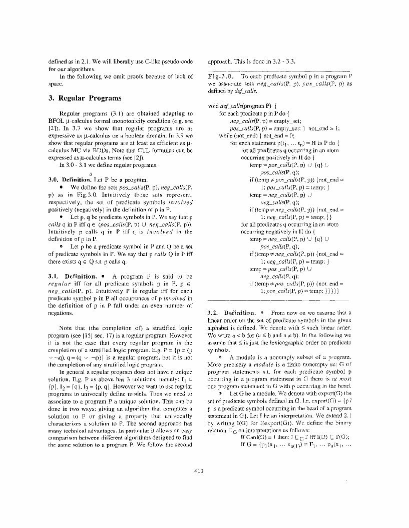
3.0. Definition. Let P be a prograim. We define the sets pos-c,dCs(P, p), neg-.calls(P,

p) as in Fig.3.0. Intuitively these sets represent, respectively, the set of predicate symbols involved positively (negatively) in the definition of p in P.

Let p, q be predicate symbols in P. We say that p calls q in P iff q E (pos-culls(P, 13) U neg-calls( Intuitively p calls q in P iff CI 11s involved definition of p in P.

Let p be a predicate symbol in P and of predicate symbols in P. We say that p calls there exists q E Q s.t. p calls q.

0

*

*

3.1. Definition. * A program F" is said to be regu lar iff for all predicate symbols p in P, p 4: neg-calZs(P, p). Intuitively P is regular iff for each predicate symbol p in P all occunrences of p involved in the definition of p in P fall under an even number of negations.

Note that (the completion of) a stratified logic program (see [15] sec. 17) is a regular program. However it is not the case that every regular program is the completion of a stratified logic program E.g. P = [p = (p v -,q), q = (q v -p)} is a regulair program, but it is not the completion of any stratified logic program.

In general a regular program does not have a unique solution. E.g. P as above has 3 solutions, namely: I, = [p}, I2 = {q}, I3 = {p, q}. However we want to use regular programs to univocally define models. Thus we nee associate to a program P a unique solution. This can be done in two ways: giving an algiorithm that computes a solution to P or giving a property that univocally characterizes a solution to P. The second approach has many technical advantages. In particular it allows an easy comparison between different algorithms designed to find the same solution to a program P. We follow the second

approach. This is done in 3.2 - 3.3.

defined by def-calls.

void def-calls(prograr

neg-culls(P, p> = empty-set; pos-calls(P, p) = empty-set; } not-end = 1;

for each statement p(t1, . . . en) = H in P do { Ifor all predicates q occurring in an atom occurring positively in

temp = pos-cuZls(P, p) U { q} U

while (not-end) { not-end = 0;

] 'XX-CU.h(P, q); if (temp f J B Q S - C U h (

I; pos-calZs(P, p) = temp; 1

1; neg-culls(P, p) = temp; } 1 for all predicates q occurring in an atom occurring negatively in H do {

tempi = neg-culls(P, p) U {q} U

t e q = ~ Q S - C U Z ~ S ( P , p) U aeg-calls(P, q);

if (temp f pos-caZls( 1 ; pos_calls(P, p) = temp; 1 } } ] }

3.2. From now on we assume that a linear set of predicate symbols in the given alphabet is defined. We denote with I such linear order. We write a < b for (a S b and a f b). In the following we assume ihat 5 is just the lexicographic order on predicate

A module is a ~ ~ n e m p ~ y subset of a program. ore precisely a module is a finite nonempty set C of

program statements s.t. for each predicate symbol p occurring in a program statement in C there is ut most one program statement in C with p occurring in the head.

e denote with expork(6) the set of predicate symbols defined in G. I.e. export(6) = p is a predicate symbol occurring in thc he statement in G}. Let 1 be an interpr by writing I(G) for H(export(G)). relation on inierpretations as follows:

If Card(G) = 1 then: 1

symbols. Q

G I' iff I(6) C I'(G); If G = ( g q ( X 1 , ... Xa($ = F1> . . ~ P n ( X l 9 ...

4111

xa(,)) = n > 1, p1 < ... < pn and M = G - {pl(xl, ... xa(l)),= F1) then: I CG I' iff (I(p1) C I'(p1) and (I(p1) = B'(p1) implies H M 1')).

Let P be a program, p be a predicate symbol in P be a set of program statements in P. We denote

with def(P, p> the definition of p in P. I.e. def(P, p) is the unique statement in P in which p occurs in the head. We define: cluster(P, p) = { def(P, p)} U { def(P, q) I (p calls q

nd (q calls p in P)}, clusters(P) = {cluster(P, p) I p }, base(P, G) = {p I (p is a predicate in P) and (p

expore(6)) and (there exists g E export(G) s.t. g calls p in

Let P be a program. A standard solution to P is an interpretation I s.t.: H k P and I = I(Alph(P)) and for all G E clusters(P), for all interpretations I', if I(base(P, G)) U 1'(G) b G then I

P?).

1'.

eorem Let P be a regular program. Then P has exactly one standard solution.

r o o f . ( S k e t c h ) . We give a constructive proof exploiting Tarsky-Knaster fixpoint theorem. See appendix A for more details.

3. ~ Let P = {q = 7p, p = p]. P is a re (as well as the completion of a stratified logic program). The standard solution to P is I = { q].

Let P = (p = (p v Tq), q = (q " Yp)}. P is a regular program. The standard solution to P is I = {q}.

Y

m, k)

3.5. Definition. * Let P be a regular program. We denote with stdsol(P) the standard solution to P. By 3.3 stdsol(P) is well defined. Let p be a predicate symbol in P. We write bdd(P, p) for bdd(stdsol(P)(p)).

A query is a pair (P, g), where P is a regular program and g is a predicate symbol in P. Answer-Query is a function from queries to Boole s.t. Answer-Query(P, g) = 1 iff stdsol(P) I= g(x1, ... xn) . Thus Answer-Query(P, g) = Answer-MC(stdsol(P), g(x1, . . . x,)). We call Answer-Query(P, g) the answer to query (P, g) and the problem of computing Answer-Query the query (evaluation) problem. Note that in this situation P is often seen as a deductive database (see [IS] sec. 21).

*

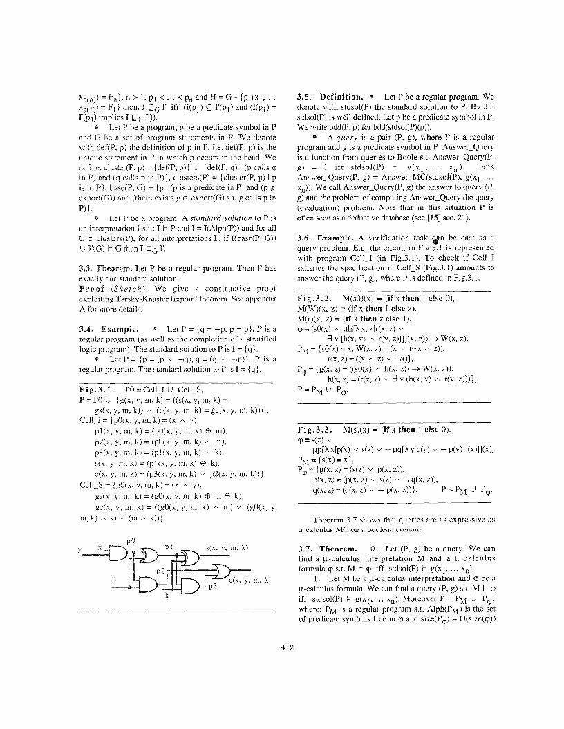
3.6. Example. A verification task query problem. E.g. the circuit in Fig. with program Cell-I (in Fig.3.1). To check if Cell-I satisfies the specification in Cell-S (Fig.3.1) amounts to answer the query (P, g), where P is defined in Fig.3.1.

Theorem 3.7 shows that queries are as expressive as pcalculus MC on a boolean domain.

3.7. Theorem. 0. Let (P, g) be a query. We can find a p-calculus interpretation M and a p-calculus formula cp s.t. M b cp iff stdsol(P) k g(x1, ... xn).

Let M be a p-calculus interpretation and cp be a p-calculus formula. We can find a query (P, g) s.t. M k cp iff stdsol(P) k g(x1, ... x,). Moreover P = PR/~ U Pp, where: PM is a regular program s.t. Alph(PM) is the set of predicate symbols free in cp and size(P9) = O(size(cp))

1.

412

(size(q) is the number of symbols in q). . (Sketch) 0. Trivial. Take ~p g(x1, ... xn) and

I . Defining M and cp in P (see example 3.8). See = stdsol(P).

appendix B for more details.

le. Let M, 9, P, PM, E' be as in Fig.3.2 or Fig.3.3. Then M != cp iff stdsol(P)l? g(x, z).

Since we are on a Boolean Domain stdsol(P) and ry are computable. HLowever to get an ifier we need to show that Answer-query is

efficiently computable. Theorem 3.9 shows that query evaluation is at least as efficient as p-calculus MC via BDDs. In particular we have BDD based algorithms for query evaluation.

. Let (P, g) be a query and let Alph(P) = There are BDD based algorithms

bdd-compile, bdd-eval s.t.: bdd-compile(P) = (bdd(P, ]PI), ... bdd(P, pk)). Answer-Query(P, g) = bdld--eval(bdd(P, PI), . . .

roof. (Ske tch ) Function bdd-compile is obtained implementing with BDDs the algorithm in the proof of 3.3. E.g. if Card(P) = 1 then bdd--compile is similar to

OINT in [2] sec. 4. Since g E Alph(P) bdd-eval simply tests if bdd(P, g) represents the boolean function

ically equal to 1. This is done in constant time since s are a canonical representation for boolean functions.

, pk), g) = bdd-eval(bdd-compile(P), g),

0. From theorem 3.9 follows that s can be imported in a query evaluation

framework. E.g. to improve fixpoint computations we can use 121 sec. 5, [ll], [16], [I31 in (tlhe proof of 3.3 and thus in) bdd-compile in 3.9.

Regular programs and queries define a BFOL based functional programming language that we call BFP (Boolean Functional Programming). Theorem 3.3 and Answer-Query (3.5) define a semantics for BFP. Theorem 3.9 defines a BDD based compiler for BFP. Note that a regular program is (the completion of) a logic program (see [15] sec. 17). Thus syntactically BFP is a Logic Programming Language. However computationally BFP is a Functional Programming Language. In fact query evaluation is carried out with a BDD based computation (bdd-eval). Thus for BFP BDDs play the same role as 1 - calculus in traditional functional programming.

From theorem 3.7 follow:, that a p-calculus MC problem (M, cp) can be cast as a query problem (P, g). Thus, using queries, systems and system specifications are represented (in P) using the same language (namely

I .

2.

BFOL). We will exploit this feature by means of program transformations.

Fa s

So far we have just shown that query evaluation is as good as I'VE. However the interest of query evaluation for automatic verification relies on the possibility of using program transformdons to avoid state explosion. This makes query evaluaiion more efficient program transformation is a map 'taking a qu returning an (hopefully) eas i e r que Answer-Query(P, g ) =: Answer-Query(P', (4.2,4.3) an easy and effective program transformation.

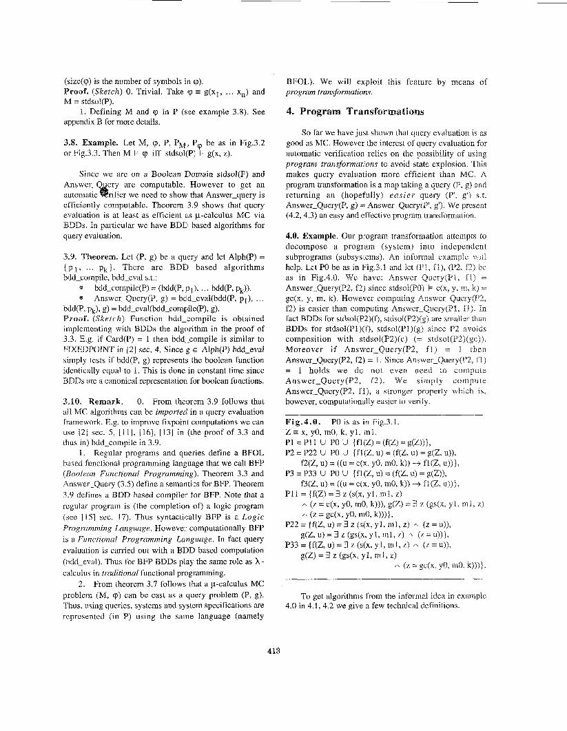
4.0. Example. Our program transformation attempts to decompose a program (system) into independent subprograms (subsystems). An informal exampic: '<ra .iI

help. Let PO be as in lFig.3.1 and let (PI, f l ) , (P2, f2) be as in Fig.4.0. We

fa) is easier than con fact BDDs for stdsol(F BDDs for stdsol(P1)i composition with s Moreover if Answer-Query(P2, f l ) = 1 iben Answer-Query(P2, f2 = 1 holds we dol not even need to compute Answer--Query(P2, f2). We simply compute Answer-iQuery(P2, f l ) , a stronger property which is, however, computationally easier tc verify.

Fig.4.8. Z z x, YO, mO, k, y1, m l .

P2 = P22 U PO U { f l (Z , U> = (f(Z, U) = g(Z, U)),

PO is as in Fig.3.1.

P1 =P11 U PO U {fl(Z)=(f(Z)=g(Z))),

P3 = P33 U PO U { fl (Z, U) = (f(Z, U) = g(Z)),

P11 = ( f ( Z ) = 3 z ( s ( x , y l , m l , z )

f2(Z, U) = ((U = c(x, yo, mO, k)) 3 fl(Z, U))},

f3(Z, U) = ((U = c(x, YO, mO, k)) -+ fl(Z, U))),

A (Z = C(X, YO, mO, k))), g(z) = 3 z (gs(x, YP, A (z = gc(x, YO, m O , k)))J,

P22 = {f(Z, U) = 3 z (s(x, y l , ml , z) A (z = U)), g(Z, u) = 3 z (gs(.rc, y l , m l , z) A (z = U)?),

P33 = {f(Z, U) = 3 z (9(x, yl , m l , z) A (z = U)), g(Z> = 3 z (gs(x, y l , nil, z>

A (z = gc(x, yo, m@ NI)).

To get algorithms from the informal idea in example 4.0 in 4.1, 4.2 we give a few technical definitions.

413

itioira, Let P be a program. predicate symbol p in P is said to be almost ff for each statement q(xl, . . . xn) = IF in P, if

(p occurs in an atom E% occurring in F) then (B = p(xl, . . . xh) and h 5 0).

A predicate symbol p in P is said to be G O L (Gate Output Like) in P iff p is almost GOL in P and for

P we have: if (q calls p in P)

Predicate symbols defining gate outputs are GOL. E.g. the following predicate symbols are GOL: s, g in P in Fig.3.1; SO, W, g in P in Fig.3.2; f, g, c, gc, f l in Pi in Fig.4.0. Predicate symbols defining operators (e.g. IC's, transition relations, transitive closures) are not GOQ. E.g. thc following predicate symbols are not GOL: s (IC) i n PI in Fig.4.0; r (transition relation), h (transitive closure) in P in Fig.3.2.

4

.4,1a Let S = {p l , ... pk}. Let u l , ... uk be fresh

variables. Choose arbitrarily functions rp, 8 : { I , . . . k} -+ { 1, ... k] s.t.: (for all i, j E 11, . . k } [ ~ ( i ) = 90) iff stdsol(P) b

a l l i ~ { c p ( j ) I j ~ { I , ... k } ) [cp(O(i))=i]). Note that we can use bdd(P, p1 1, . . . bdd(P, pk) to test

if stdsol(P) b pi(xI, . . . x ~ ( ~ ) ) = pj(xl, . . , xbci)) holds. @ S) and (there is no p

E S s.t. p cillls q in P) and (q calls S in P)) then 1 else 0. Note that if refreshed(P, S , q) = 1 then q is GOL in P.

refresh(P, S, {U,, ... uk}) = P', where P' is obtained from P as follows:

For all statements q(xl, . . . xh) = F in P s. t. refreshed(P, S, q) = 1 replace q(xl , ... x,,) =

F with q(xl ' ... xh) = F', where F' is obtained from F by replacing, for i = 1, . .. k, pi(xl , . . . xb($ in F with u .

cp(l).

For all atoms q(xl , ... xh) s.t.

refreshed($, S, q) = 1 replace q(xl, . . . xh) in P with q(xl,

reduce-quer);(P, g, S) = (refresh(P, S , {U, , ...

U ] , . . . uk)) 1, g'), where: (note that refreshed(P, S, g) = 1 and that g i s GOL in P)

g' is a fresh predicate symbol, { cp(j) I j E { 1,

... Xbii)) = p.(x 1, ... ~ ~ ~ $ 1 ) and (for

refreshed(P, S , q) = if ((9

0

Step 6.

Step 1.

. . . Xh' u i ~ . . . Uk) .

@

"k)) U {g'(xl, ... Xn' u1' ... uk) = (G g(x,. ... x,,

... k ) ] = {p( l ) , ... p(r)}, G = ((U p(1) = PS(p(l))(Xl> ' ' .

xb(O(p(l))))) A ..'

~ n ~ v o c a ~ ~ y defined. This, however, will be harmless.

= b ( p ( r ) ) ( x l ' .'. 'b(O(p(r)))))). Note that, strictly speaking, reduce-query is not

A (P, g)-redex (4.2.0) is a set S of predicate symbols in P that can be replaced with fresh variables. The new query (PI> E') obtained from (P, g) via S is computed from P, g, S by reduce-query (4.2.1). A similar idea has been used in A-calculus to solve systems of equations (e.g. see ~51, [a [181).

efinition. 0. Let (P, g) be a query. A nonempty set S of GOL predicate symbols in P is said to be a (P, g)-redex iff ( ( g e S) and (g calls S,& P) and (there is no p E S s.t. p calls g in P)).

Let (P, g) be a query and S be a (P, g)-redex. Function reduce-query is defined as in Fig.4.1. E.g. consider example 4.0 again. Then {c, gc} is a (Pl , f1)- redex and (P2, a) = reduce-query(P1, f l , { c , gc}).

,,*e

1 .

Theorem 4.3.0 shows that from a (P, g)-redex S and reduce-query we get a program transformation. Theorem 4.3.1 shows that a counter-example ( 0 ) for reduce-query(P, g, S) is also a counter-example for (P, g) *

4.3. Theorem. Let (P, g) be a query, S be a (P, g)- redex and (PI, g') = reduce-query(P, g, S) .

Answer-Query(P, g) = Answer-Query(P, g'). For each state G, if [stdsol(P'), ol(g'(x1, ... x,~))

= 0 then [stdsol(P), ol(g(x1, .. . x,)) = 0. Proof. (Sketch) . Using the following fact. Since all predicates in S are GOL in P we have: (see definition of reduce-query in Fig.4.1) for all predicate symbols q in P, if refreshed(P, S, q) = 1 then q is GOL in P.

0. 1 .

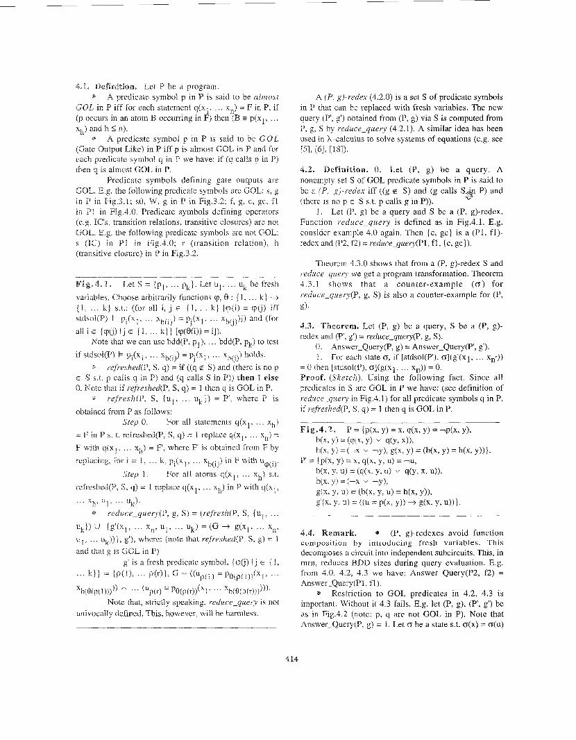
F i g . 4 . 2 . p = {p(x, y) = x, q(x, y> =1p(x , y), b(x, Y) = (q(x, Y) " Y(Y, x)), h(x, Y) = (- " lY) , g(x, Y) = (Wx, Y) = h(x, YN}.

P' = {P(& y) = x, q(x, y, U) = IU, b(x, Y, U) = (q(x, Y, U) " 0, x, U)), h(x, y) = (TX v -y>, g(X, Y: U> = (b(x, Y , U) = N x , Y>>, g'(x, Y 3 U) = ((U = P(% Y)) + g(x, Y > U))}-

emark. * (P, g)-redexes avoid function composition by introducing fresh variables. This decomposes a circuit into independent subcircuits. This, in turn, reduces BDD sizes during query evaluation. E.g. from 4.0, 4.2, 4.3 we have: Answer-Query(P2, f2) = Answer-Query(P1, f l ) .

Restriction to GOL predicates in 4.2, 4.3 is important. Without it 4.3 fails. E.g. let (P, g), (P, g') be as in Fig.4.2 (note: p, q are not GOL in P). Note that Answer-Query(P, g) = 1. Let o be a state s.t. o(x) = ~ ( u )

@

4 14

= 1, o(y) = 0. Then [stdsol(P'), c~](g'(x, y, U)) .- 0 (but [stdsol(P), o](g(x, y)) = 1). Thus Answer-Query(P, g) # Answer-Query(P, g').

(P, g)-redexes only act on predicate symbols that are GOL. Thus non-GOL predicatle symbols represent non-decomposable subsystems (of the system defined by P). Our program transformation cannot prevent state explosion caused by non-decomposable subsystems. This means that our program transformation is effective on systems obtained connecting together not-too-large non- decomposable subsystems. In particular (P, g)-redexes are effective on combinatorial circuits built from not-too- l a r g e IC's. Note that no MC automatic global optimization technique working on combinatorial circuits is available.

A verification problem is ani MC problem (M, cp) in an MC setting and a query (P, g) in a BFP setting. All algorithms used in an MC setting can be imported in a BFP setting (see 3.10.0). However not all BFP optimization techniques can be easily exported to an MC setting. E.g. 4.2, 4.3 cannot be used in an MC setting since M and cp are defined using different languages. Defining systems and specifications in the same language (BFOL) is the main advantage of using BFP as an automatic verifier.

5. Reduction Strategy

Given a query (P, g) in general not all (P, g)-redexes will improve query evaluation performances. Thus we need an efficient reduction strategy, i.e. an algorithm that given a query (P, g) returns a reasonably good (P, g)- redex S whithin a reasonable time. Note that (if P # NP) we cannot expect to make all queries easy.

In this section we give an efficient reduction strategy (5.4) aimed to avoid function Composition in a program. This reduces BDD sizes during query evaluation. Note that this is not the only possible criterion to choose a reduction strategy, but it is an effective one (see sec. 6).

Given a query (P, g) there are O(2size(P)) sets of GOL predicates to be considered as rede.x candidates. We cannot consider all of them. Thus we restrict our search to safe redexes (5.1). Example 5.0 motivaCes restriction to safe redexes.

The point is that redex {c} avoids composition with predicate: symbol c, but does not avoid composition with function stdsol(P3)(c) since stdsol(P3)(c) = stdsol(P3)(gc).

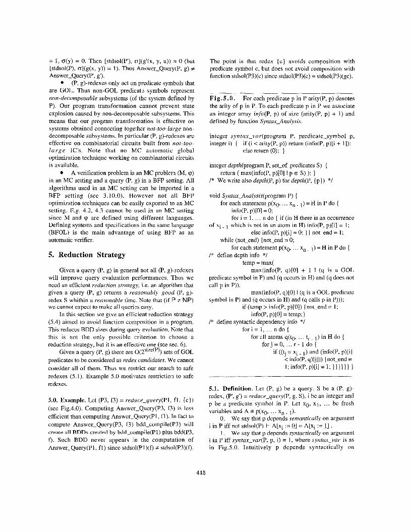
Fig .5 . (11. For each predicate p in P arity(P, p) denotes the arity of p in P. To each predicate p in P we associate an integer array info(P, p) of size (arity(P, p) + 1) and defined by function S,yntax-Analysis.

integer .syntax-var(program P, predicate-symbol p, integer i)l { if (i < arity(P, p)) return (info(P, p)[i + 11);

else return (0); }

integer depth(progran-i P, set-of-predicates S) { return ( max(info(P, p)[O] I p E S) ); }

/* We write also depi%(P, p) for depth(P, { p}) */

void Syntax-Analysis(program P) {

info(P, p)[O] = 0; for i = 1, . . . n do { if (in H there is an occurrence

for each statement p(x0, . . . x, - 1) = H in P do {

of xi - 1 which is not in an atom in H) info(P, p)[i] = 1; else info(P, p)[i] = 0; } } not-end = 1;

while (not-end) { not-end = 0; for each statement p(x0, . . . x, 1) = H in P do {

/* define depth info */ temp = max(

max(info(P, q)[O] + 1 I (q is a GOL predicate symbol in P) and (q occurs in H) and (q does not call p in P)),

maxi(info(P, q)[O] I (q is a GOL predicate symbol in P) and (q occurs in H) and (q calls p in P)));

info(P, p)[O] = temp;} /* define syntactic dependency info */

if (temp > info(P, p)[O]) {not-end = 1;

fori = 1, ... n do { for all atoms q(t0, . . . t, - 1) in H do {

for j=O, ... r - 1 d o { if ((tj = xi - 1) and (info(P, p)[i]

< info(P, q)Q])) { not-end = 1; info(P,p)[iI = 1; }}I}}} }

5.1. Definition. Le:t (P, g) be a query, S be a (P, 8)- redex, ( P I , 8') = reduce-query(P, g, S), i be an integer and p be a predicate syiinbol in P. Let xo, XI, ... be fresh variables and A ~ p(xo, . . . xn -

We say that p depends semantically on argument i in p iff not stdsol(P) k A[x; := Q] = A[xi := 1 1 .

5.0. Example. Let (P3, f3) = reduce-query(P1, f l , {c}) (see Fig.4.0). Computing Answer-Query(P3, f3) is less efficient than computing Answer-Query(P1, fl). In fact to compute Answer-Query(P3, f3) bdd-compile(P3) will

0.

create all BDDs created by bdd-compile(P1) plus bdd(P3, We say that p depends syntactically on argument f). Such BDD never appears in the computation of i in P i f syntax-var(P, p, i) = 1, where syntax-var is as Answer-Query(P1, f l ) since stdsol(Pl)(f) # stdsol(P3)(f). in Fig.5.O. Intuitively p depends syntactically on

1 .

415

argument i iff xi is involved in the definition of p in P.

satisfying the following conditions:

argument i in P';

2. S is said to be safe iff there exists an integer i

@ For all p E S , p depends semantically on

g does not depend syntactically on i in P'. E.g. consider example 4.0 again. Then {e, gc} is

a safe (Pl, f1)-redex, whereas {c} is not (see 5.0).

The following proposition shows that safe redexes avoid situations like the one described in example 5.0.

ition. Let (P, g) be a query, S be a safe (P, (P, g') = reduce-query(P, g, S).

if ((4 is g) or (g calls q in P')) then not stdsol(P') != p(x0,

roof. (Sketch). Showing that for any regular program P the following facts hold. (0) If p in P depends semantically on argument i in P then p depends syntactically on argument i in P. (1) If p depends semantically on argument i in P and q does not depend syntactically on argument i in P then not stdsol(P) k

For all p E S, for all GOL predicates q in P,

. x, - 1) = q(x07 . . . xb - 1).

P(x0, ... x, - 1 ) = q(x@ ... Xb - 1).

ark. We can efficiently decide if a given redex is safe. In fact let (Pi g) be a query. We note the following. (0) To efficiently decide if p in P depends semantically on argument i we can use BDDs. It suffices to check if the index corresponding to argument i of p occurs in bdd(P, p). This can be done traversing bdd(P, p). Thus semantic dependency can be decided in time O(size-bdd(bdd(P, p))). (1) To efficiently decide if p in P depends syntactically on argument i we use Syntax-Analysis in Fig.5.O (no BDDs needed).

Unfortunately predicate symbols in a safe redex can easily generate large BDDs. Thus to avoid state explosion we only consider safe redexes built from GOL predicates which definition is not too complex. Function depth (see Fig.5.0) defines our measure of complexity for predicate symbol definitions. We only consider safe redexes which predicate symbols have depth less than a given integer. Theorem 5.4 shows that for such redexes there is an efficient reduction strategy (reduce-step).

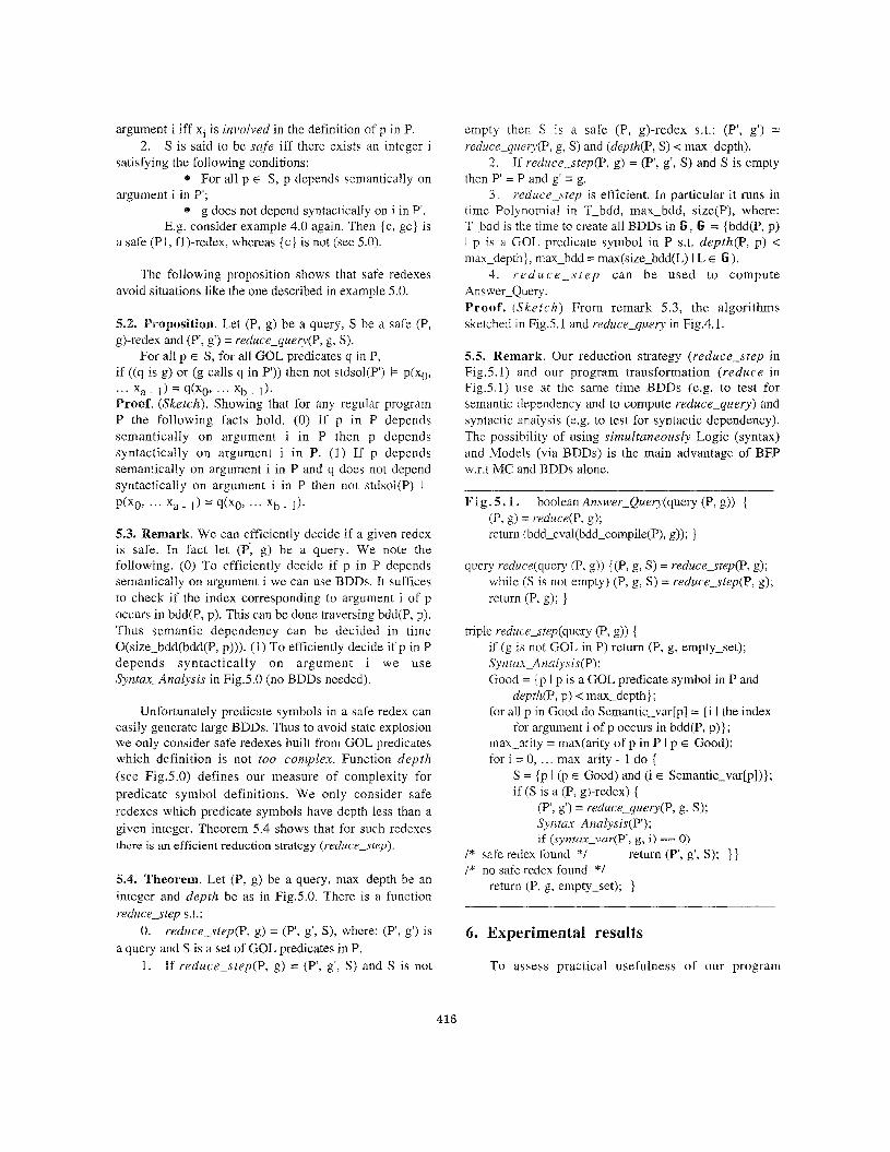
5.4. Theorem. Let (P, g) be a query, max-depth be an integer and depth be as in Fig.5.0. There is a function reduce-step s. t. :

reduce-step(P, g) = (PI, g', S), where: (PI, g') is a query and S is a set of GOL predicates in P.

If reduce-step(P, g) = (PI, g', S) and S is not

0.

1.

empty then S is a safe (P, g)-redex s.t.: (E", g') = reduce-quety(P, g, S) and (depth(P, S) < max-depth).

2. If reduce-step(P, g) = (PI, g', S) and S is empty then P' = P and g' = g.

3. reduce-step is efficient. In particular it runs in time Polynomial in T-bdd, max-bdd, size(P), where: T-bdd is the time to create all BDDs in G , G = { bdd(P, p) I p is a GOL predicate symbol in P s.t. depth(P, p) < max-depth}, max-bdd = max(size-bdd(L) I L E E).

4. r e d u c e - s t e p can be used to compute Answer-Query . Proof. (Sketch) From remark 5.3, the algorithms sketched in Fig.5.1 and reduce-query in Fig.4.1.

5.5. Remark. Our reduction strategy (reduce-step in Fig.5.1) and our program transformation (reduce in Fig.5.1) use at the same time BDDs (e.g. to test for semantic dependency and to compute reduce-query) and syntactic analysis (e.g. to test for syntactic dependency). The possibility of using simultaneously Logic (syntax) and Models (via BDDs) is the main advantage of BFP w.r.t MC and BDDs alone.

Fig . 5 . 1 . boolean Answer-Query(query (P, g)) { (P, g) = reduce(P, g); return (bdd-eval(bdd-compile(P), g)); }

query reduce(query (P, g)) { (P, g, S) = reduce-step(P, g); while (S is not empty) (P, g, S) = reduce-step(P, g); return (P, g); }

triple reduce-step(query (P, g)) { if (g is not GOL in P) return (P, g, empty-set); Sy n tax-A nu ly s is (P) ; Good = { p I p is a COL predicate symbol in P and

depth(P, p) < max-depth}; for all p in Good do Semantic-var[p] = { i I the index

for argument i of p occurs in bdd(P, p)}; max-arity = max(arity of p in P I p E Good); for i = 0, . . . max-arity - 1 do {

S = {p I (p E Good) and (i E Semantic-var[p])}; if (S is a (P, g)-redex) {

(P, g') = reduce-query(P, g, S); Syntax-A naly s is (PI) ; if (syntau_var(P', g , i) == 0)

/* safe redex found */ return (PI, g', S); } } /* no safe redex found *I

return (P, g, empty-set); }

6. Experimental results

To assess practical usefulness of our program

416

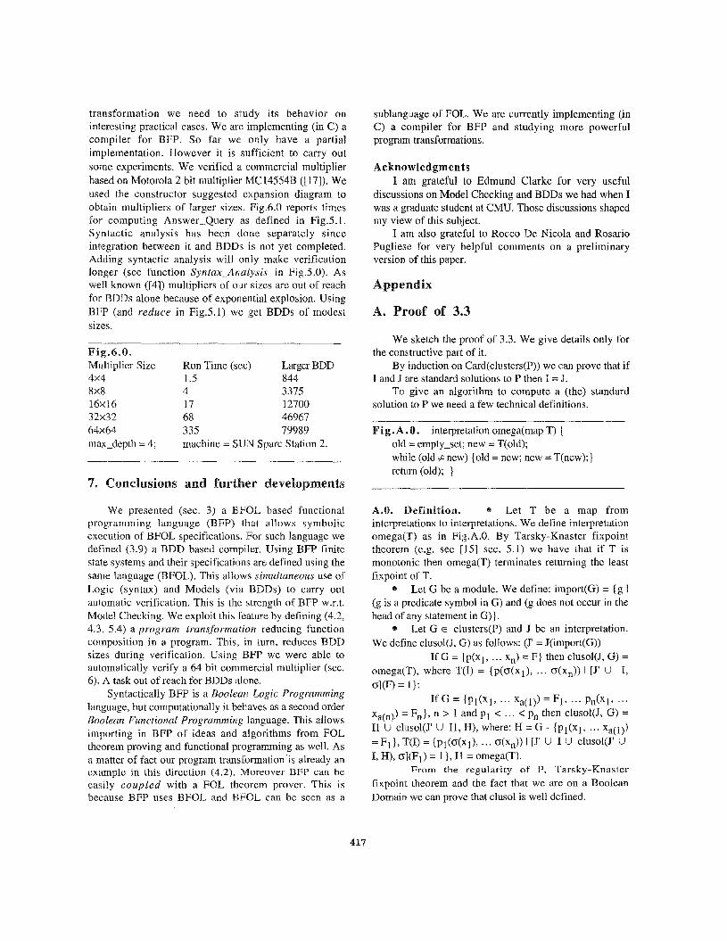
transformation we need to study its behavior on interesting practical cases. We are implementing (in C ) a compiler for BFP. So far we only have a partial implementation. However it is sufficient to carry out some experiments. We verified ai commercial multiplier based on Motorola 2 bit multiplier R4C14554B ([17]). We used the constructor suggested expansion diagram to obtain multipliers of larger sizes. Fig.6.0 reports times for computing Answer-Query as defined in Fig.5.1. Syntactic analysis has been done separately since integration between it and BDDs is not yet completed. Adding syntactic analysis will only make verification longer (see function Syntax-Analysis in Fig.5.O). As well known ([4]) multipliers of our sizes are out of reach for BDDs alone because of exponential explosion. Using BFP (and reduce in Fig.5.1) wie get BDDs of modest sizes.

Multiplier Size Run Time (sec) Larger BDD 4x4 1.5 844 8x8 4 3375 16x16 17 12700 32x32 68 4696'7 64x64 335 79989 maxdepth = 4; machine = SUN Sparc Station 2.

We presented (sec. 3) a BFOL based functional programming language (BFP) that allows symbolic execution of BFOL specifications. For such language we defined (3.9) a BDD based compiler. Using BFP finite state systems and their specifications are defined using the same language (BFOL). This allows simultaneous use of Logic (syntax) and Models (via BDDs) to carry out automatic verification. This is the strength of BFP w.r.t. Model Checking. We exploit this feature by defining (4.2, 4.3, 5.4) a program transformation reducing function composition in a program. This, in turn, reduces BDD sizes during verification. Using EiFP we were able to automatically verify a 64 bit commercial multiplier (sec. 6). A task out of reach for BDDs alone.

Syntactically BFP is a Boolean Logic Programming language, but computationally it behaves as a second order Boolean Functional Programming language. This alIows importing in BFP of ideas and algorithms from FOL theorem proving and functional programming as well. As a matter of fact our program transformation is already an example in this direction (4.2). Moreover BFP can be easily coupled with a FOL theorem prover. This is because BFP uses BFQL and NFOL can be seen as a

sublanguage of FOL. We are currently implementing (in C ) a compiler for BFP and studying more powerful program transformations.

Acknowledgments I am grateful to Edmund Clarke for very useful

discussions on Model Checking and BDDs we had when I was a graduate student at CMU. Those discussions shaped my view of this subjlect.

I am also grateful to Rocco De Nicola and Rosario Pugliese for very helpful comments on a preliminary version of this paper.

We sketch the proof of 3.3. We give details only for

By induction on Card(clusters(P)) we can prove that if

To give an algorithm to compute a (the) standard

the constructive part of it.

I and J are standard solutions to P then I = J.

solution to P we need a few technical definitions.

Fig . A . 0. interpretation omega(map T) { old = empty-set; new = T(o1d); while (old # new) {old = new; new = T(new);} retuim (old); }

lefinition. @ Let T be a map from interpretations to interpretations. We define interpretation omega(T) as in Fig.A.O. By Tarsky-Knaster fixpoint theorem (e.g. see [15] sec. 5.1) we have that if T is monotonic then omega(T) terminates returning the least fixpoint of T.

Let G be a module. We define: import((;) = {g I (g is a predicate symbol in G) and (g does not occur in the head of any statement in G)}.

Let G E clusters(P) and J be an interpretation. We define clusol(J, G) as follows: (J' = J(import(G))

If G = (p(x1, . . . xn) = F} then clusol(J, G) = omega(T), where T(1) = {p(o(xl), ... o(xn)) I [J' U I,

*

0

ol(F) = 11;

x ~ ( ~ ) ) =: F,], n > 1 ,and p1 < . . . < pn then clusol(J, 6) = I1 U clnsol(J' U 11, H), where: H = G - { p ~ ( x ~ , ... ~ ~ ( 1 ) )

I, H), o](F1) = l}, I1 = omega(T). From the regularity of P, Tarsky-Knaster

fixpoint theorem and the fact that we are on a Boolean Domain we can prove that clusol is well defined.

If G = { P I ( x ~ , ... ~ ~ ( 1 ) ) F1, ... pn(xl, ...

= F~ 1, *r(I) = { p ] ( ~ ( ~ ~ ) , ... o(~,)) I [J' U I U ciusoi(r U

417

We define the interpretation sol(P) as follows: If clusters(P) = {G} then sol(P) = clusol(0, G); If Card(clusters(P)) > 1 then sol(P) = sol(P -

G ) U clusol(sol(P - G), G), where: G is an arbitrarily chosen module in clusters(P) s.t. there is no p in (P - G) s.t. p calls export((;) in P. Note that Card(clusters(P - G)) < Card(clusters(P)), thus sol(P) is well defined.

We can prove that sol(P) in A.0 is indeed a standard solution to P. This concludes the proof of 3.3.

B. Proof of 3.7.3

We sketch the proof of 3.7.1. We give details only for the constructive part of it. We follow p-calculus definition in [2]. Note that we call individual variables and relational variables in [2], respectively, variables and predicate symbols. Let free-pred(cp) be the set of predicate symbols free in cp. W.1.o.g. we can assume that M = M(free-pred(cp)) (see 2.1). Thus M defines a finite set of boolean functions. Since boolean functions can be defined using regular programs we can easily find a regular program PM s.t. stdsol(PM) = M. To define Pq we need a few technical definitions.

B.Q. Definition. * Let FH be a map from natural numbers to predicate symbols not occurring in cp or PM s.t.: for all i, k E N, if i < k then FH(i) < FH(k).

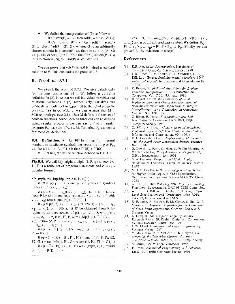
* Let mu-bfp be the function defined in Fig.B.0.

Fig.B.Q. We call bfp-triple a triple (i, P, cp) where: i E

I N , P is a finite set of program statements and cp is a p- calculus formula.

bfp-triple mu-bfp(bfp-triple (i, P, cp)) { if (cp = p(x1, ... xn) and p is a predicate symbol)

return (i, P, p(xl, . . . x,)); if (cp = ? X I , ... x,[F](yl, ... y,)) {let F be obtained

from F by simultaneously replacing XI, . . . xn in F with y l , ... yn; return (mu-bfp(i, P, F')); }

if (cp = pp[R](xl, ... x,)) {let FV((p) = {zl , ... Zk, x1, ... xn}; p' = FH(i); let R' be obtained from R by replacing all occurrences of p(t1, . . . tn) in R with p'(t1, ... I,, z1, ... zk); (i', P , F) = mubfp(i c 1, P, R'(xl, ... xn)); return (it, P' U {p'(xl, ... x,, z l , ... zk) = F}, p'(x1,

if (cp = F) { (i', P', F') = mu-bfp(i, P, F); return (i', P', 1 F); }

if (cp = F v G) { ( i l , P1, F1) = mu-bfp(i, P, F); (i2, P2, 6 1 ) = mu-bfp(i1, P1, 6); return (i2, P2, F1 v GI); }

if (cp = 3 z [F]) { (i', P , F ) = mu-bfp(i, P, F); return

e . . xn, z], ... zk)); }

(i', P', 3 z CF'I); 1 1

Let (i, PI, F) = mu-bfp(0, 0, cp). Let FV(F) = {XI, . . . xn} and g be a fresh predicate symbol. We define: PQ = P1 U {g(xl, . . . xn) = F}, P = PM U P . Finally we can prove 3.7.1 by induction on size(cp).

References

cp

K.R. Apt, Logic Programming, Handbook of Theoretical Computer Science, Elsvier 1990 J. R. Burch, E. M. Clarke, K. L. McMillan, D. L. Dill, L. J. Hwang, Symbolic model checking: 1020 states and beyond, Information and Computation 98, (1 992) R. Bryant, Graph-Based Algorithms for Boolean Function Manipulation, IEEE Transaction on Computers, Vol. C-3.5, N.8, Aug. 1986 R. Bryant, On On the complexity of VLSI Implementations and Graph Representations of Boolean Functions with Application to Integer Multiplication, IEEE Transaction on Computers, Vol. 40, N.2, Feb. 1991 C. Bohm, E. Tronci, X-separability and Left- Invertibility in A -calculus, LICS 1987, IEEE Computer Society, 1987 C. Bohm, E. Tronci, About systems of equations, X-separability and Lef-Invertibility in A -calculus, Information and Computation, 90, (1991) R. L. Constable et altri, Implementing Mathematics with the Nuprl Proof Develpment System, Prentice- Hall, 1986 G. Dowek, A. Felty, G. Huet, C. Paulin-Mohring, B. Werner, The Coq Proof Assistant user's guide 5.6, INRIA-Rocquencourt, 134, 1991 E. A. Emerson, Temporal and Modal Logic, Handbook of Theoretical Computer Science, Elsvier 1990 M. J. C. Gordon, HOL: a proof generating System for Higher Order Logic, in VLSI Specification, Verification and Synthesis, Kluwer SECS 3.5, Kluwer, 1988 A. J. Hu, D. Dill, Reducing BDD Size by Exploiting Functional Dependencies, DAC 93, IEEE Comp. Soc. A. J. Hu, D. Dill, A. J. Drexler, C. H. Yang, Higher Level Specification and Verification using BDDs, CAV 92, to be reprinted in LNCS D. E. Long, A. Browne, E. M. Clarke, S. Jha, W. R. Marrero, An Improved Algorithm for the Evaluation of Fixed Point Expressions, CAV 94, LNCS 818, Springer-Verlag L. Lamport, The Temporal Logic of Actions, Research Report 79, Digital Equipment Corporation, Systems Research Center, Dec. 1991 J. W. Lloyd, Foundations of Logic Programming, Springer-Verlag 1987 Y. Matsunaga, P. C. McGeer, R. K. Brayton, On computing the Transitive Closure of a State Transition Relation, DAC 93, IEEE Comp. Society. Motorola, CMOS Logic Databook, I986 E. Tronci, Equational Programming in A-calculus, LICS 1991, IEEE Computer Society, 1991

418