Hardware-Software Co-design of Resource-EfficientDeep Neural Networks

byHokchhay Tann

M.Sc., Brown University, Providence, RI, 2016B.Sc., Trinity College, Hartford, CT, 2014

A dissertation submitted in partial fulfillment of therequirements for the degree of Doctor of Philosophy

in School of Engineering at Brown University

PROVIDENCE, RHODE ISLAND

May 2019

© Copyright 2019 by Hokchhay Tann

This dissertation by Hokchhay Tann is accepted in its present formby School of Engineering as satisfying the

dissertation requirement for the degree of Doctor of Philosophy.

Recommended to the Graduate Council

Date

Sherief Reda, Advisor

Date

Jacob Rosenstein, Reader

Date

Rodrigo Fonseca, Reader

Approved by the Graduate Council

Date

Andrew G. Campbell, Dean of the Graduate School

iii

Vitae

Hokchhay Tann was born and raised in Pursat Province, Cambodia. He received his

B.Sc. with double majors in Engineering (EE Concentration) and Mathematics from Trin-

ity College, Hartford, CT in 2014. He received his M.Sc. in Electrical and Computer

Engineering from Brown University in 2016 during his studies in the Ph.D. program. His

main areas of research include approximate computing, resource-efficient design and ac-

celerations of neural networks with applications to iris recognition and chemical compu-

tation.

hokchhay tann@brown.edu

https://www.htann.com

Brown University, RI, USA

Selected Publications:

1. H. Tann, H. Zhao, S. Reda, “Resource-Efficient Embedded Iris Recognition Systems

Using Fully Convolutional Neural Networks,” under revision in ACM Journal of

Emerging Technologies in Computing Systems (JETC), 2019.

2. K. Nepal, S. Hashemi, H. Tann, R. I. Bahar and S. Reda, “Automated High-Level

Generation of Low-Power Approximate Computing Circuits,” in IEEE Transactions

on Emerging Topics in Computing, vol. 7, no. 1, pp. 18-30, 1 Jan.-March 2019.

3. C. Arcadia, H. Tann, A. Dombroski, K. Ferguson, S. L. Chen, E. Kim, B. Ruben-

iv

stein, C. Rose, S. Reda and J. Rosenstein, “Parallelized Linear Classification with

Volumetric Chemical Perceptrons,” in IEEE International Conference on Rebooting

Computing (ICRC), 2018, pp. 1-9.

4. S. Hashemi, H. Tann, and S. Reda, “BLASYS: Approximate Logic Synthesis Using

Boolean Matrix Factorization,” in ACM/ESDA/IEEE Design Automation Confer-

ence (DAC), 2018, pp. 1-6.

5. S. Hashemi, H. Tann, F. Buttafuoco and S. Reda, “Approximate Computing for Bio-

metric Security Systems: A Case Study on Iris Scanning,” in Design, Automation

& Test in Europe Conference & Exhibition (DATE), 2018, pp. 319-324.

6. H. Tann, S. Hashemi, R. I. Bahar and S. Reda, “Hardware-software codesign of

accurate, multiplier-free Deep Neural Networks,” in ACM/EDAC/IEEE Design Au-

tomation Conference (DAC), Austin, TX, 2017, pp. 1-6.

7. S. Hashemi, N. Anthony, H. Tann, R. I. Bahar and S. Reda, “Understanding the

impact of precision quantization on the accuracy and energy of neural networks,” in

Design, Automation & Test in Europe Conference & Exhibition (DATE), Lausanne,

2017, pp. 1474-1479.

8. H. Tann, S. Hashemi, R. I. Bahar and S. Reda, “Runtime configurable deep neu-

ral networks for energy-accuracy trade-off,” in International Conference on Hard-

ware/Software Co-design and System Synthesis (CODES+ISSS), Pittsburgh, PA,

2016, pp. 1-10.

Book Chapters:

1. H. Tann, S. Hashemi, and S. Reda, “Lightweight Deep Neural Network Accelerators

Using Approximate SW/HW Techniques,” in Approximate Circuits, pp. 289-305.

Springer, 2019.

v

2. H. Tann, S. Hashemi, and S. Reda, “Approximate Computing for Iris Recognition

Systems,” in Approximate Circuits, pp. 331-348. Springer, 2019.

3. S. Hashemi, H. Tann, and S. Reda, “Approximate Logic Synthesis Using Boolean

Matrix Factorization”, in Approximate Circuits, pp. 141-154. Springer, 2019.

Technical Report

1. H. Tann, S. Hashemi, S. Reda, “Flexible Deep Neural Networks Processing,” arXiv

Technical Report, 2018.

vi

Acknowledgements

This thesis would not have been possible without the inspirations, support and mentoring

from many kind individuals, for whom I am forever grateful. First and foremost, I would

like to express my immense gratitude to my advisor and mentor, Prof. Sherief Reda, for

his guidance, support and insights. I would also like to thank Prof. Jacob Rosenstein and

Prof. Rodrigo Fonseca for being on my defense committee and taking the time to review

my thesis.

I am extremely thankful for the fruitful collaborations with all my co-authors, Prof. Iris

Bahar, Prof. Jacob Rosenstein, Dr. Soheil Hashemi, Heng Zhao, Francesco Buttafuoco,

Chris Arcadia, Nicholas Anthony, Dr. Kumud Nepal, my advisor Prof. Sherief Reda, and

many others. My work would not have been possible without them. Specifically, I would

like to thank Dr. Soheil Hashemi for being an incredible collaborator and friend.

I would like to thank all my friends at Brown, who made my time here a wonderful one.

Thank you to all my friends and colleagues in SCALE lab: Kapil Dev, Xin Zhan, Reza

Azimi, Onur Ulusel, Sofiane Chetoui, Farnaz Nouraei, Marina Hesham, Abdelrahman

Ibrahim, Abdelrahman Hussein and many others for always making the lab a fun place to

be at. Thank you Pratistha Shakya, Chen Lin and the Khmer Student Association for fun

parties and gatherings.

I would like to thank Yicheng Shao (Dora) for the years of support, encouragements,

insightful discussions, and many unforgettable memories.

vii

Last but not least, I would like to thank my parents, Toumneup Tann and Mouyly

Taing, and my siblings for their unwavering support and love. I have learned a lot from

them. Without them, none of what I achieved today would be possible.

The research in this thesis is partially supported by NSF grants 1420864, 1814920,

and DARPA W911NF-18-2-0031.

viii

Abstract of “Hardware-Software Co-design of Resource-EfficientDeep Neural Networks” by Hokchhay Tann, Ph.D., Brown University, May 2019

The unprecedented success of deep learning technology has elevated the state-of-the-art

accuracy performance in many application domains such as computer vision and voice

recognition. At the same time, typical Deep Neural Network (DNN) models used in

deep learning contain hundreds of millions of parameters and require billions of expensive

floating-point operations to process each input. The large storage and computational over-

heads severely limit DNN’s applicability on resource-constrained systems such as mobile

and embedded platforms.

Recently, a large number of resource optimization techniques and dedicated hardware

architectures have been proposed to alleviate these overheads. The principal observation

enabling such optimization approaches stems from the inherent error-resilient property of

DNNs, where approximation-induced accuracy loss can be potentially recovered through

retraining or finetuning. In addition, applications deploying DNNs in their processing

pipeline tend to be resilient to small inaccuracies in the output produced by DNNs. With

the growing importance of the field of machine learning and the increasing number of

embedded systems, the success of DNN approximation techniques would be critical to

enable resource-efficient operations.

This thesis makes several contributions toward advancing the progress of DNN in-

ference on embedded platforms. First, we introduce design methodologies to reduce the

hardware complexities of DNN models and propose light-weight approximate accelerators

that can efficiently process these models. Our methodologies include analysis and novel

training algorithms for a spectrum of data precisions ranging from fixed-point, dynamic

fixed point, powers-of-two to binary data precision for both the weights and activations

of the models. We demonstrate custom hardware accelerator designs for the various data

precisions which achieve low-power and low-latency while incurring insignificant accu-

ix

racy degradation. To boost the accuracy of the proposed light accelerators, we describe

ensemble processing techniques that use an ensemble of light-weight DNN accelerators to

achieve the same or better accuracy than the original floating-point accelerator. We also

introduce two flexible runtime strategies, which enable significant savings in DNN infer-

ence latency. Our methodologies are flexible in that they allow for dynamic adaptation

between the quality of results (QoR) and execution runtime. First, we present a novel dy-

namic configuration technique that permits adjustments in the number of channels in the

network depending on response time, power, and accuracy targets. Our second runtime

technique enables flexible inference for DNNs ensembles, which is a popular and effective

method to boost the inference accuracy.

Next, we showcase our DNN design methodologies using an end-to-end iris recogni-

tion application. Here, we propose a resource-efficient end-to-end iris recognition flow,

which consists of FCN-based segmentation, contour fitting, followed by Daugman nor-

malization and encoding. To obtain accurate and efficient FCN architectures, we intro-

duce a SW/HW co-design methodology, where we propose multiple novel FCN models.

Incorporating each model into the end-to-end flow, we show that the recognition rates

of our end-to-end pipelines outperform the previous state-of-the-art on the two datasets

evaluated. To further simplify the models for efficient inference, we quantize the weights

and activations of the models to dynamic fixed-point (DFP) format and propose a DFP

accelerator. We realize our HW/SW co-design pipeline on an embedded FPGA platform.

Finally, we extend our work to emerging computing paradigms for machine learning

by introducing a novel methodology for a chemical-based single-layer neural network.

We propose a parallel encoding scheme which simultaneously represents multiple bits in

microliter-sized chemical mixtures. While the demonstration is still limited in scale, we

consider this as a first step to building computing systems that can complement electronic

systems for applications in ultra-low-power systems and extreme environments.

x

Contents

Vitae iv

Acknowledgments vii

1 Introduction 1

1.1 Problem Characterization . . . . . . . . . . . . . . . . . . . . . . . . . . 1

1.2 Major Thesis Contributions . . . . . . . . . . . . . . . . . . . . . . . . . 4

2 Background 8

2.1 Deep Neural Networks . . . . . . . . . . . . . . . . . . . . . . . . . . . 8

2.2 Hardware-Software Co-design of Deep Neural Networks . . . . . . . . . 12

3 Hardware-Software Co-design of Deep Neural Network Accelerators 15

3.1 Introduction . . . . . . . . . . . . . . . . . . . . . . . . . . . . . . . . . 15

3.2 Data Precision Options . . . . . . . . . . . . . . . . . . . . . . . . . . . 17

3.3 Hardware Accelerator Designs . . . . . . . . . . . . . . . . . . . . . . . 20

3.4 Training For Low Precision Networks . . . . . . . . . . . . . . . . . . . 23

3.5 Boosting Accuracy with Ensemble Processing . . . . . . . . . . . . . . . 27

3.6 Experimental Results . . . . . . . . . . . . . . . . . . . . . . . . . . . . 28

3.7 Conclusion . . . . . . . . . . . . . . . . . . . . . . . . . . . . . . . . . 32

4 Runtime-Flexible Deep Neural Networks Processing 34

4.1 A Dynamically Configurable DNN Design . . . . . . . . . . . . . . . . . 35

x

4.1.1 Introduction . . . . . . . . . . . . . . . . . . . . . . . . . . . . . 35

4.1.2 Background . . . . . . . . . . . . . . . . . . . . . . . . . . . . . 36

4.1.3 Methodology . . . . . . . . . . . . . . . . . . . . . . . . . . . . 37

4.1.4 Runtime Methodology . . . . . . . . . . . . . . . . . . . . . . . 42

4.1.5 Experiments . . . . . . . . . . . . . . . . . . . . . . . . . . . . . 48

4.1.6 Experimental Setup . . . . . . . . . . . . . . . . . . . . . . . . . 48

4.1.7 Conclusions . . . . . . . . . . . . . . . . . . . . . . . . . . . . . 59

4.2 A Flexible Processing Strategy for DNN Ensembles . . . . . . . . . . . . 59

4.2.1 Introduction . . . . . . . . . . . . . . . . . . . . . . . . . . . . . 59

4.2.2 Related Works . . . . . . . . . . . . . . . . . . . . . . . . . . . . 61

4.2.3 Methodology . . . . . . . . . . . . . . . . . . . . . . . . . . . . 62

4.2.4 Experimental Results . . . . . . . . . . . . . . . . . . . . . . . . 66

4.3 Conclusion . . . . . . . . . . . . . . . . . . . . . . . . . . . . . . . . . 68

5 Resource-Efficient Fully Convolutional Networks for Iris Recognition Ap-plication 69

5.1 Introduction . . . . . . . . . . . . . . . . . . . . . . . . . . . . . . . . . 69

5.2 Background and Related Works . . . . . . . . . . . . . . . . . . . . . . . 72

5.2.1 Traditional Iris Segmentation Methodologies . . . . . . . . . . . 73

5.2.2 Fully Convolutional Networks for Iris Segmentation . . . . . . . . 75

5.2.3 Metrics for Iris Segmentation Accuracy . . . . . . . . . . . . . . 76

5.3 Proposed Methodology . . . . . . . . . . . . . . . . . . . . . . . . . . . 78

5.3.1 Fully Convolutional Networks Architecture Design . . . . . . . . 79

5.3.2 Segmentation Accuracy Evaluations . . . . . . . . . . . . . . . . 82

5.3.3 Quantization to Dynamic Fixed-Point . . . . . . . . . . . . . . . 85

5.3.4 End-to-end FCN Models Evaluation . . . . . . . . . . . . . . . . 86

5.4 Implementation of Iris Recognition Pipeline on Embedded SoC . . . . . . 89

5.4.1 Runtime Profiles for Iris Recognition Pipeline . . . . . . . . . . . 89

xi

5.4.2 FCN Processing Components . . . . . . . . . . . . . . . . . . . . 91

5.4.3 Hardware Accelerator Architecture . . . . . . . . . . . . . . . . . 92

5.5 Experimental Results . . . . . . . . . . . . . . . . . . . . . . . . . . . . 95

5.5.1 Experimental Setup . . . . . . . . . . . . . . . . . . . . . . . . . 95

5.5.2 Recognition Performance Evaluations and Comparisons . . . . . 95

5.5.3 Runtime Performance and Hardware Acceleration Speedup . . . . 100

5.6 Conclusion . . . . . . . . . . . . . . . . . . . . . . . . . . . . . . . . . 102

6 Co-Design Techniques for Chemical-based Neural Classifier 104

6.1 Introduction . . . . . . . . . . . . . . . . . . . . . . . . . . . . . . . . . 104

6.2 Proposed Chemical Computing Methodology . . . . . . . . . . . . . . . 106

6.2.1 Encoding Data in Chemical Mixtures . . . . . . . . . . . . . . . 106

6.2.2 Computing with Chemical Mixtures . . . . . . . . . . . . . . . . 108

6.2.3 Reading the Results of Chemical Mixture Computations . . . . . 111

6.3 System Development . . . . . . . . . . . . . . . . . . . . . . . . . . . . 112

6.3.1 Experimental Setup . . . . . . . . . . . . . . . . . . . . . . . . . 112

6.4 Experiments & Results . . . . . . . . . . . . . . . . . . . . . . . . . . . 113

6.4.1 Robustness Simulation . . . . . . . . . . . . . . . . . . . . . . . 114

6.4.2 MNIST Image Classification . . . . . . . . . . . . . . . . . . . . 115

6.4.3 Performance Evaluation . . . . . . . . . . . . . . . . . . . . . . 116

6.5 Conclusion . . . . . . . . . . . . . . . . . . . . . . . . . . . . . . . . . 118

7 Summary of Dissertation and Possible Future Directions 119

7.1 Summary of Results . . . . . . . . . . . . . . . . . . . . . . . . . . . . . 120

7.2 Potential Research Extensions . . . . . . . . . . . . . . . . . . . . . . . 123

Bibliography . . . . . . . . . . . . . . . . . . . . . . . . . . . . . . . . . . . 124

xii

List of Figures

2.1 The structure of a neuron (perceptron). . . . . . . . . . . . . . . . . . . . 9

2.2 The structure of a typical DNN. . . . . . . . . . . . . . . . . . . . . . . . 9

3.1 The hardware architecture of our accelerator. . . . . . . . . . . . . . . . 20

3.2 Architecture of Neural Processing Unit for uniform fixed-point activations.The pipeline consists of three main blocks: weight block (WB), addertree (AT), and non-linearity unit (NL). The weight block can be modifiedaccording to different weight quantization schemes. . . . . . . . . . . . . 21

3.3 Architecture of Neural Processing Unit for dynamic fixed-point precision. 23

3.4 Training procedure for DNNs with reduced-precision parameters. . . . . . 24

3.5 Ensemble Processing. . . . . . . . . . . . . . . . . . . . . . . . . . . . . 28

3.6 The Pareto Frontier plot of the evaluated design points for CIFAR-10dataset. The X-axis is shown in logarithmic scale to cover the large en-ergy range of all the designs. Here, the black point indicates the initial32-bit floating-point design. . . . . . . . . . . . . . . . . . . . . . . . . . 31

3.7 Accelerator area utilization for different precision formats normalized againstthe 32-bit floating-point reference design. . . . . . . . . . . . . . . . . . 32

4.1 Illustration of Incremental Training on a typical DNN. . . . . . . . . . . . 38

4.2 Dynamic adjustment of DNN capacity using feedback controllers as im-plemented in the proposed constrained design approach. For real time con-straints, the controller monitors the response time and power consumptionof the DNN and adjusts its capacity based on the measurements and thetarget runtime constrains. . . . . . . . . . . . . . . . . . . . . . . . . . . 43

4.3 Dynamic adjustment of DNN capacity using score margin classifiers asimplemented in the proposed opportunistic approach. The score marginunit scales down the DNN to save energy as long as accuracy is not com-promised. . . . . . . . . . . . . . . . . . . . . . . . . . . . . . . . . . . 44

xiii

4.4 Inference accuracy of golden model in validation set versus relative net-work runtime in forward pass. . . . . . . . . . . . . . . . . . . . . . . . 46

4.5 Histogram for top two class scores margin for correct inference (top) andwrong inference (bottom) for CIFAR-10 dataset. The number of channels(x/y) shows the ratio of number of channels in the first layer of the networkin use (x) and that of the full network (y). This ratio is identical for alllayers except the final layer. . . . . . . . . . . . . . . . . . . . . . . . . . 48

4.6 The custom HW implemented in our work. . . . . . . . . . . . . . . . . . 49

4.7 Comparison of inference accuracy on CIFAR-10 validation set for goldenmodel, incremental training, channel increments shutdown and incremen-tal training with initialization from Section 8. Relative runtime is the ratioof the forward-pass runtime to that of the full network. The two num-bers displayed at each datapoint (x/y) shows the number of channels asexplained in Figure 4.5. . . . . . . . . . . . . . . . . . . . . . . . . . . . 53

4.8 Test set inference accuracy versus network relative runtime for MNIST(top), SVHN (middle), and CIFAR-10 (bottom). The two numbers (x/y) ateach data point have the same representation as Figure 4.5. . . . . . . . . 54

4.9 Comparison of network energy adjusts with the imposed energy budgetover time running MNIST tesebench. . . . . . . . . . . . . . . . . . . . . 57

4.10 Inference accuracy versus average runtime per input for AlexNet and ResNet-50 for DNN ensembles on ImageNet validation set. Each data label showsthe number of networks in the ensemble. Runtime results are based on asystem with a Nvidia Titan Xp GPU. . . . . . . . . . . . . . . . . . . . . 62

4.11 Score Margins histograms for correct and wrong top-1 inference for AlexNet.The x-axis shows the score margin, and the y-axis shows the number ofsamples in each score margin bin. . . . . . . . . . . . . . . . . . . . . . 65

4.12 Execution flow for flexible DNN ensemble processing. . . . . . . . . . . 65

4.13 Inference accuracy versus average runtime per input for AlexNet and ResNet-50 for normal and flexible ensemble execution. Runtime results are basedon a system with a Nvidia Titan Xp GPU. . . . . . . . . . . . . . . . . . 67

5.1 Typical processing pipeline for iris recognition applications based on Daug-man [19]. . . . . . . . . . . . . . . . . . . . . . . . . . . . . . . . . . . 73

5.2 Architecture for Encoder-Decoder Fully Convolution Networks with skipconnections for semantic segmentation. . . . . . . . . . . . . . . . . . . 75

xiv

5.3 F-measure segmentation accuracy and computational complexity of can-didate FCN models on CASIA Iris Interval V4 and IITD datasets. Themodels use 32-bit floating point for both weights and activations. Thescales refer to the ratio of the model input dimensions to the originalimage resolutions from the datasets. Smaller resolution inputs can sig-nificantly reduce the computational complexity of the models. We labelmodels which make up the Pareto fronts as FCN0-FCN8 for CASIA4 andFCN9-FCN19 for IITD. . . . . . . . . . . . . . . . . . . . . . . . . . . . 83

5.4 Processing pipeline for contour fitting, normalization and encoding. . . . 87

5.5 FCN-based iris recognition pipeline runtime breakdown for floating-pointFCN0–FCN8 models from CASIA Interval V4 Pareto front in Figure 5.3.From left to right, the FCN models are arranged in increasing computa-tional complexity. Results are based on floating-point FCN models. . . . . 90

5.6 Image to column operation for convolution layer. . . . . . . . . . . . . . 92

5.7 Overall system integration and the hardware accelerator module for theGEMM unit. The code representing the operations of the hardware mod-ule is shown in the bottom left, where A and B are the multiplicant andmultiplier matrices, and C is the resulting output matrix. For DFP versionof the accelerator, A and B are 8-bit, and C is 16-bit. A, B and C areall 32-bit floats for the floating-point version. The accelerator module isconnected to the Zynq Processor Unit via the Accelerator Coherency Port(ACP). . . . . . . . . . . . . . . . . . . . . . . . . . . . . . . . . . . . . 93

5.8 A closer look at the data paths of the buffers in the DFP accelerator unit. . 94

5.9 Receiver Operating Characteristic (ROC) curves of FCN-based iris recog-nition pipelines with ground truth segmentation and different floating-point FCNs models for CASIA Interval V4 and IITD datasets. In the leg-end of each dataset, the FCN models are arranged in increasing FLOPsfrom bottom to top. The zoom-in axis range is [0 0.02] for both x and ydirections. . . . . . . . . . . . . . . . . . . . . . . . . . . . . . . . . . . 97

5.10 Runtime results for end-to-end FCN-based iris recognition pipelines basedon different FCN segmentation models for the IITD dataset. Five plat-form configurations are reported: pure none-vectorized floating-point soft-ware (SW Float), vectorized float-point and fixed-point software usingARM NEON instructions (SW Vectorized Float, SW Vectorized DFP) andhardware accelerated with floating-point and DFP acceleerators (SW+HWVectorized Float, SW+HW Vectorized DFP). The speedup relative to SWFloat is reported on top of each bar. . . . . . . . . . . . . . . . . . . . . . 100

5.11 FPGA floorplans of our synthesized accelerators and system modules. . . 102

xv

6.1 A conceptual block diagram of the chemical computation scheme. Binarydatasets are encoded into discretized mixtures of chemicals. Computa-tions can be performed on these chemical mixtures through quantitativesampling, based on the desired classifier’s weights, and mixing of theircontents. The computation output is initially still in the chemical domain,and can be assessed using analytical chemistry techniques. Figure fromArcadia et al. [6]. . . . . . . . . . . . . . . . . . . . . . . . . . . . . . . 106

6.2 Data is stored in isolated wells containing quantitative chemical mixtures.The concentrations of these chemicals reflect the values of the binary inputdata. Each bit address in the input data is assigned to one grid location ona microplate, while the value of each bit is encoded in the concentrationof a particular chemical compound at that position. Multiple datasets canbe simultaneously stored in the same fluid containers by using multipledistinct chemicals. Figure from Arcadia et al. [6]. . . . . . . . . . . . . . 107

6.3 A schematic of the proposed chemical computation procedure, as im-plemented for pattern classification. All spatially concurrent chemicaldatasets (x) are operated on in parallel by a single weight matrix (w),whose values are realized as volumetric fluid transfers. Since weightscan be positive and negative (wi ∈ [−1, 1]), a pool for each polarity ismade. Each pool is analyzed by liquid chromatography to measure theconcentrations of each analyte species. The differential concentration ofeach analyte is calculated in post-processing and used to determine theappropriate label for the input data. Figure from Arcadia et al. [6]. . . . . 109

6.4 An overview of the experimental setup and data flow used for these exper-iments. Weight matrices were trained in simulation and then converted,along with test data, into sequences of pipetting instructions for a roboticliquid handler. Analytes were dispensed into a 384-well microplate toform the chemical dataset and then collected in volume fractions corre-sponding to the classifier weight matrix. The outputs were analyzed byHPLC to produce class labels. Figure from Arcadia et al. [6]. . . . . . . . 112

6.5 Single-layer neural network classification simulation results. Figure (a)shows the classification error introduced from the varying uncertainties inimage creation portion while assuming the volumetric multiply-accumulateand HPLC readings are assumed to be exact. For Figure (b), the volumeuncertainty for image creation was fixed at 0.05 while varying the un-certainties in the multiply-accumulate pooling volumes. The HPLC con-centration reading was assumed to be exact. For each data point in bothfigures, the mean and standard deviation are computed from a trial of 100runs. . . . . . . . . . . . . . . . . . . . . . . . . . . . . . . . . . . . . . 115

xvi

6.6 Chemical classification of MNIST handwritten digits. Three 16×16 (256-bit) binary images were chemically encoded, in parallel, on a 384-wellplate. The overlaid chemical images were then classified by a three-neuron,single-layer neural network which had been previously trained to identifyeither digit ‘0’, ‘1’, or ‘2’. The results of this experiment are shown in atable format as class matches (zm > 0) or mismatches (zm < 0). All ninechemical classifier outputs were correct (3 true positives, 6 true negatives)(shown in (a)). A photograph of the microplate containing the chemicaldataset of overlaid images is also shown in (b). Each well in the plate con-tains 60µL of liquid whose chemical composition represents the values ofone pixel across three images. Figure from Arcadia et al. [6]. . . . . . . . 116

6.7 Validation experiments for chemical classifiers with pseudo-random data.Sixteen trials were performed. In each trial, three 16-bit data vectors(x1, x2, x3) were chemically encoded and classified according to a weightvector (w). The computed class label (`) is shown for each vector, alongwith a green check mark or red cross out to indicate whether or not thechemical classifier identified it correctly. In total, 46 out of 48 vectorswere correctly classified (96% accurate with 2 false positives). Figurefrom Arcadia et al. [6]. . . . . . . . . . . . . . . . . . . . . . . . . . . . 117

xvii

List of Tables

3.1 Classification accuracy, inference time, and energy cost for CIFAR-10 andImageNet benchmark DNNs based on different numerical representationand ensembling. Ensemble deployment uses two DNNs in the inference.Accuracy results show Top-1 performance and Top-5 in parentheses forImageNet benchmark. . . . . . . . . . . . . . . . . . . . . . . . . . . . . 30

4.1 The hardware implementation characteristics of different arithmetic andbit-widths. . . . . . . . . . . . . . . . . . . . . . . . . . . . . . . . . . . 50

4.2 Breakdown of hardware implementation characteristics of different com-ponents. . . . . . . . . . . . . . . . . . . . . . . . . . . . . . . . . . . . 51

4.3 Benchmark Networks Architecture Descriptions. . . . . . . . . . . . . . 52

4.4 Mean energy cost (E) and processing time (T) per input image when differ-ent fractions of the each networks are deployed using our custom hardwareaccelerator. . . . . . . . . . . . . . . . . . . . . . . . . . . . . . . . . . 55

4.5 Mean energy cost (E) and processing time (T) per input image when differ-ent fractions of the each networks are deployed using Nvidia Jetson TX1GPU board. Input images are fed into the network one at a time. . . . . . 56

4.6 Additional storage requirements normalized to the original network whenthe system is allowed to store multiple weights network. . . . . . . . . . . 57

4.7 Optimal number of retraining increments for each network and fractionsof active channels in each layer for each increment (score margin thresholdin parentheses). . . . . . . . . . . . . . . . . . . . . . . . . . . . . . . . 58

4.8 Inference Accuracy (in parenthesis is the accuracy of the golden modelfor network with the same size as the increment) and energy cost for eachincrement in incremental training. . . . . . . . . . . . . . . . . . . . . . 58

4.9 Energy savings and accuracy drops for the dynamic configuration normal-ized to the golden result. . . . . . . . . . . . . . . . . . . . . . . . . . . 59

xviii

5.1 Proposed baseline FCN architecture. Each convolution layer (CONV) isfollowed by Batch Normalization and ReLU activation layers. Transposedconvolution layer (TCONV) is followed by ReLU activation layer. Thearrows denote the skip connections, where the outputs of two layers areadded together element-wise before passing to the next layer. VariableN denotes the number of feature maps per layer, which is varied amongdifferent designs explored. . . . . . . . . . . . . . . . . . . . . . . . . . 80

5.2 Segmentation Accuracy Comparison to Previous Works . . . . . . . . . . 84

5.3 Descriptions of FCN architectures and their computational complexities(MFLOPs) which achieve top segmentation accuracy among all modelsexplored in Figure 5.3 for CASIA Interval V4 and IITD datasets. As in Ta-ble 5.1, each CONV layer is followed by Batch Normalization and ReLU,and TCONV is followed by ReLU. FS denotes the filter size, and the skipconnections are represented by the arrows. . . . . . . . . . . . . . . . . . 85

5.4 Runtime profile for floating-point FCN inference using the onboard CPU. 90

5.5 Equal Error Rate (EER) and segmentation accuracy (F-measure) compari-son between previous approaches, our FCN-based pipeline and groundtruth(GT). In each dataset, FCN models are floating-point based and arrangedin increasing FLOPs and F-measure from top to bottom. . . . . . . . . . 98

5.6 Equal Error Rate (EER) and segmentation accuracy (F-measure) compar-ison between the groundtruth (GT), floating-point, and DFP FCN-basedrecognition pipelines using the IITD dataset. . . . . . . . . . . . . . . . . 99

5.7 Utilization of FPGA Resources for Look-up Tables (LUT), LUT as mem-ory (LUTRAM), Flip-Flop Registers, Block RAM (BRAM), Digital Sig-nal Processing units (DSP), and Global Clock Buffers (BUFG). . . . . . . 101

6.1 Computational cost of classifying M binary inputs, each containing Nbits, in a traditional versus volumetric neuron . . . . . . . . . . . . . . . 108

xix

Chapter 1

Introduction

1.1 Problem Characterization

Machine learning has become an integral part of many systems we interact with. From

data centers to embedded devices, machine learning models are deployed to enable var-

ious services such as language translations, voice recognition, and recommendation en-

gines. With the recent breakthroughs in deep learning [56, 32], we are capable of solving

ever more complex tasks, many of which were not previously possible. The ability to auto-

matically learn important features from large datasets distinguishes deep learning models,

also known generally as deep neural networks (DNNs), from previous machine learning

techniques, which rely on handcrafted feature extractors. In order to capture essential fea-

tures and their underlying relationships from large and complex datasets, state-of-the-art

DNNs typically consists of hundreds of millions of trainable parameters, hyperparameters

and require millions of expensive computations for each input.

The success in deep learning has been possible in part due to the performance leaps

1

achieved in modern computing systems. As accurately predicted by Gordon Moore in

1965, Moore’s law states that the number of transistors in dense integrated circuits roughly

doubles every 18 months [67]. This is due to the continual downsizing of the transistor

area, which improves the circuit performance by allowing for higher switching frequency.

In addition, the observation from Robert Dennard in 1974, known as the Dennard scal-

ing, stated that with the shrinking of the transistor feature size, the operating voltage and

current would be downscaled proportionally and that the power density would remain

constant [21]. Combining of Moore’s Law and Dennard scaling, this meant that the per-

formance per watt of integrated circuits would double every 18 months paving way for an

incredible semiconductor roadmap. However, more recently, we have reached the end of

Dennard scaling and soon Moore’s Law. In order to keep up the momentum, the indus-

try and academic research have looked for other directions such as parallelized multicore

systems and building more specialized circuits, i.e. accelerators and Application-Specific

Integrated Circuits (ASIC), for various tasks and integrate them as a system on a chip

(SoC) [22, 23].

In addition, as we target more and more challenging tasks, it is expected that the com-

plexities of DNN models will continue to grow dramatically. In order to continue the

progress in deep learning, efficient high-performance computing systems and methodolo-

gies are among the essential components. This need is evidenced in recent work such as

neural architecture search [104], which deployed 800 Graphics Processing Units (GPU)

concurrently. For this reason, a thriving field of research in both academia and industries

focuses on designing specialized, efficient hardware architectures to support the immense

computational requirements of DNNs. Some of the popular systems currently deployed to

train and run large DNNs models from industries include the deep-learning tailored GPUs,

Tensor Processing Unit (TPU) [51] and Fields-Programmable Gate Array (FPGA).

Another line of research focuses on the deployments of DNN models in more resource-

2

constrained environments, which are mobile and embedded systems. With the ubiquity of

these platforms, they have become popular target systems for many deep learning appli-

cations. However, these systems are often battery-powered with limited computational

resources and strict power budgets making the deployments of large DNN models chal-

lenging. This problem has motivated many studies which focus on designing specialized,

efficient hardware architectures and software-hardware co-design approaches to support

the computational need of DNNs while simultaneously meeting the system constraints

[15, 16, 31, 99]. A large number of software-hardware co-design approaches were pro-

posed to reduce the complexities of DNN models through sparsification [60], bit-width

reduction [34], as well as exploring more efficient model architectures [44, 47]. Others

have proposed low-power, small-footprint accelerator designs which can support many of

the simplified DNNs models [15, 16, 100, 35]. Collectively, these various techniques have

shown promising results in achieving an orders-of-magnitude reduction in the number of

arithmetic operations, runtimes, and power requirements.

The impressive improvements from the proposed optimization techniques are often re-

alized by trading off small accuracy loss of the models for large savings in computational

overhead. However, this accuracy loss is often measured through certain test sets with iso-

lated DNNs. In many end-to-end applications, DNNs are often just one of the components

in the processing pipeline. Thus, the isolated accuracy loss measurements may not reflect

the true performance of the optimization methodologies on the end-to-end applications. It

is vitally important to also capture the impacts of proposed optimization techniques on the

end-to-end performance of the applications. As evidenced in the previous work [37, 90],

such end-to-end evaluation can also provide additional insights, which simplify the DNN

models.

Finally, while semiconductor-based computing systems have driven the breakthroughs

in deep learning, alternative computing paradigms, which could potentially offer more

3

flexibility as well as efficiency in computation may be necessary to help drive the progress

forward. A number of emerging technologies have been explored such as in-memory

computations, quantum computing, and chemical-based computing. These alternative

paradigms may help bring deep learning to new applications, where semiconductor-based

systems are unsuitable. Next, we provide a summary of the contributions made in this

thesis.

1.2 Major Thesis Contributions

In this section, we outline the major contributions made in this thesis with regards to

the explorations of efficient DNNs design methodologies and accelerations as well as the

emerging chemical computing domain.

1. Hardware-Software Co-design of Deep Neural Network Accelerators: In Chap-

ter 3, we propose a hardware-software co-design methodology targeting DNN accel-

erations to achieve low-power, low-latency inference with insignificant degradation

in accuracy performance. Our goal is to devise light approximate DNN accelera-

tors that use fewer hardware resources while incurring negligible accuracy loss. In

order to simplify the hardware requirements, we first perform a detailed analysis

of a broad range of data representation formats ranging from floating point to fixed

point, dynamic fixed point, powers-of-two, and binary weights and activations. To

compensate for accuracy loss due to the limited bit-precisions, we employ learning

technique which performs quantization-aware fine-tuning of the DNN parameters.

In addition, we show how to fine-tune a low-precision DNN using student-teacher

learning to improve accuracy performance in a similar manner to knowledge dis-

tillation [39]. Our technique does not require architectural change for the network.

4

We also describe how to utilize an ensemble of low-precision networks to boost

classification accuracy while still allowing large energy savings. We demonstrate

the effectiveness of our DNN accelerators through two well-known state-of-the-art

and demanding datasets, namely CIFAR-10 and ImageNet, with well-recognized

network architectures for our experiments. Our light DNN accelerators provide

dramatic savings in energy consumption in comparison to a baseline floating-point

accelerator.

2. Runtime-Flexible Deep Neural Networks Processing: The hardware-software co-

design technique proposed in Chapter 3 focuses on the design-time aspect of DNN

optimization. Once the fine-tuning process is completed, the runtime and accu-

racy of the model are fixed. While the technique significantly simplifies the DNN

models, fixed accuracy loss and runtime may not be desirable or efficient for ap-

plications with varying real-time constraints such as recommendation systems. To

enable runtime flexibility, we propose in Chapter 4, two runtime trade-off strategies

which aim to lower the average inference latency of DNN models, while maintain-

ing minimal impact on accuracy performance. Our techniques are flexible in that

they allow for dynamic adaptation between the quality of results (QoR) and execu-

tion runtime. First, in Section 4, we propose a runtime-configurable DNN design

and incremental training strategy, which allow parts of the models to be shut down

at runtime to reduce computational cost. We evaluate our proposed methods using

two different platforms: a low-power embedded GPU and a custom ASIC-based

hardware accelerator design, which uses an industrial-strength tool flow and a 65

nm technology library. Next, in Section 4.2, we propose runtime trade-off strategies

for DNN ensembles, which is a popular and effective technique to boost inference

accuracy performance. We demonstrate the effectiveness of the technique on well-

known models, which are AlexNet [56] and ResNet-50 [38] using the ImageNet

dataset [79].

5

3. Resource-Efficient Fully Convolutional Networks for Iris Recognition Appli-

cation: In Chapter 4, in order to explore the effects of DNN HW/SW co-design

methodologies on an end-to-end application, we propose an iris recognition pro-

cessing pipeline, which consists of fully convolutional neural network (FCN) based

segmentation, contour fitting, followed by Daugman normalization and encoding.

To obtain accurate and efficient FCN architectures, we employ HW/SW co-design

methodologies as proposed in Chapter 3 while introducing architectural exploration

as a first step. In this exploration, we propose multiple novel FCN models and

construct a Pareto plot based on their segmentation performance and computational

overheads. We then select the most efficient set of models and further optimizing

their HW resources by quantizing their weights and activations to 8-bit dynamic

fixed-point. We then incorporate each model into the end-to-end flow to evaluate

their true recognition performance. Compared to previous works, our FCN archi-

tectures require 50× fewer FLOPs per inference while setting a new state-of-the-art

segmentation accuracy. The recognition rates of our end-to-end pipeline also outper-

form the previous state-of-the-art on the two datasets evaluated. We then propose

a custom dynamic fixed-point accelerator and fully demonstrate the SW/HW co-

design realization of our flow on an embedded FPGA platform. In comparison with

the embedded CPU, our hardware acceleration achieves up to 8.3× speedup for the

overall pipeline while using less than 15% of the available FPGA resources.

4. A Novel Volumetric Chemical Single-Layer Neural Networks for Parallelized

Classifications: We extend our work to emerging computing paradigms for ma-

chine learning by introducing a novel methodology for the chemical-based single-

layer neural network (NN) in Chapter 6. We propose a novel encoding technique

which simultaneously represents multiple datasets in an array of microliter-scale

chemical mixtures. Parallel computations on these datasets are performed as robotic

liquid handling sequences, whose outputs are analyzed by high-performance liquid

6

chromatography. As a proof of concept, we chemically encode several MNIST

images of handwritten digits and demonstrate successful chemical-domain classifi-

cations of the digits using a volumetric single-layer NN. We additionally quantify

the performance of our method with a larger dataset of binary vectors and compare

the experimental measurements against predicted results. Paired with appropriate

chemical analysis tools, our approach can work on increasingly parallel datasets.

We anticipate that related approaches will be scalable to multilayer NNs and other

more complex algorithms.

The organization for the remainder of this thesis is as follows. Chapter 2 briefly re-

views the basics of DNNs and related works in DNN HW/SW co-design methodologies.

Next, Chapter 3 presents our proposed HW/SW co-design techniques aimed at simpli-

fying DNN designs. Chapter 4 introduces our proposed runtime-flexible methodologies

and results on well-known benchmarks. Next, in order to explore the impacts of DNN

HW/SW co-design methodologies on an end-to-end application, we present an iris recog-

nition pipeline with FCN-based segmentation in Chapter 5. In Chapter 6, we propose and

demonstrate novel parallelized single-layer NN classifier in the chemical domain. Finally,

Chapter 7 summarizes the results and findings presented in this thesis as well as offering

insights for future extensions to this work.

7

Chapter 2

Background

2.1 Deep Neural Networks

Inspired by the structure of the human brain, deep neural networks (DNNs) are proposed

as a family of machine learning models which loosely resembles the connections of the

neurons in the brain. At the core of DNNs are the neuron units, which were originally

proposed several decades ago. Beginning in the 1940s, the McCulloch-Pitts neuron [66]

was proposed, where two binary inputs are fed into a threshold function. This single

neuron unit could perform simple logical operations such as AND and OR. Building on

top of this model, Frank Rosenblatt [78] proposed the perceptron model, which could take

analog values inputs and perform a weighted sum of the inputs before passing the result

through a threshold or other kinds of non-linear functions. Figure 2.1 shows structure of

the perceptron model, and its operation can be formulated as:

y = F(n−1∑i=0

xi · wi + b),

8

∑

wnxn

w2x2

w1x1

. . .

y

Figure 2.1: The structure of a neuron (perceptron).

ConvolutionInput Pooling Classifier

Cn

C1

C1

Cn

...

Figure 2.2: The structure of a typical DNN.

where xi and wi are the i-th input feature and weights respectively, b is the bias, and F is

the non-linear function. In modern DNNs, the perceptron model is used as the core neuron

unit, where they are arranged in multiple layers. The weights in DNNs are adjusted as the

models learn to perform various tasks. Figure 2.2 shows the organization and connections

of layers in a type of DNNs, namely convolutional neural network (CNN). CNNs are

typically employed for tasks involving images or videos as inputs. Note that, while there

exists many different types of DNNs targeted for tasks from various domains, we focus

mainly on CNNs and their variants when referring to DNNs in this thesis.

With the availability of high-performance computing systems and large training datasets,

DNNs have recently produced state-of-the-art accuracy performances for many of the most

challenging problems in computer vision, such as image classification and object detec-

tion. As shown in Figure 2.2, traditional DNN architectures consist of several stacked

layers, where each layer gets its input from the previous layer and feeds its output to the

9

next layer. Here, the intermediate values between different layers are called the feature

maps. In this approach, each layer consists of a number of channels, where each channel

is responsible for implementing a specific feature map filter. Channels within a layer share

the inputs from the previous layer while each using a different set of weights.

While there is a broad range of different layers available in the literature, some of

the most common types of layers in DNNs include convolutional, pooling, and fully con-

nected layers. More recently, transposed convolution layers, also known as deconvolu-

tional layers, are also becoming prevalent due to their importance in image segmentation

and generative adversarial networks (GANs). These layers are typically followed by a

non-linear activation function. We briefly describe each layer type below.

• Convolutional Layers: Convolutional layers have multiple filters, where each filter

applies a convolution to the input feature maps. In other words, the convolutional

layer performs a weighted sum on a region of the input features. The number of

filters directly translates into the number of channels in the respective layer. The

convolution operation can be formulated as: y = b +∑

i

∑j

∑k(xi,j,k · wi,j,k).

Here, x is the input subset, w is the kernel weight matrix, and b is a scalar bias.

These layers are used for feature extractions.

• Fully Connected Layers: In this layer, each neuron has weighted synaptic connec-

tions to all neurons in the previous layer. In other words, a fully connected layer

treats its input as a 1-dimensional vector and generates a 1-dimensional vector as a

result.

• Pooling Layers: These layers extract local information in each feature map by down-

sampling input feature maps. The two most popular pooling layers are average

pooling and max pooling. These layers are commonly used to reduce the spatial

dimensions of the feature maps and help the models achieve translation invariance.

10

• Transposed Convolution Layers: These layers are used to upsample the spatial di-

mensions of the input feature maps, which are typically employed in image seg-

mentation and GANs. Transposed convolution is also known as deconvolution and

fractionally strided convolution. Compared to convolutional layers, the forward op-

erations in these layers are similar to a backward pass through convolution layers,

and the backward pass through transposed convolution is similar to the forward pass

in a convolutional layer.

• Non-Linear Activation Function: Non-linearity is necessary for DNNs as they in-

crease the decision boundaries and approximation power of the models. Without

non-linearity, stacked layers could be folded into a single layer. Currently, the most

popular non-linear function in DNNs is the rectified linear unit (ReLU).

DNNs typically are based on floating-point precision and trained with backpropagation

algorithm. Each training step involves two phases: forward and backward. In the forward

phase, the network is used to perform inference on the input. Afterward, the partial gra-

dients with respect to the loss are propagated back to each layer in the backward phase.

These partial gradients are then used to update the network parameters using stochastic

gradient descent rules. After the network is trained, it can be utilized in inference mode

to evaluate each input. In all of the state-of-the-art DNN architectures, the biggest portion

of the computational demands is required by the multiplier blocks utilized in the convo-

lutional, deconvolution and fully connected layers. We discuss next previous efforts to

reduce these computational complexities.

11

2.2 Hardware-Software Co-design of Deep Neural Net-

works

Recent interest in efficient, low-cost inference of DNNs has motivated a broad exploration

of viable algorithmic solutions, hardware designs as well as the intersection of the two,

namely hardware-software co-design. Often, these solutions take advantage of the error-

resilient nature of DNNs by trading off small accuracy loss for potentially large saving in

computational overheads. DNNs error tolerance originates from the inherently approxi-

mate nature of the applications as well as the training process of the models, where some

of the induced errors can be compensated by re-learning and fine-tuning the parameters.

We first discuss some of the existing algorithmic-based approaches aimed at simpli-

fying DNN overheads. One of the promising solutions proposed in several studies was

condensing large, cumbersome DNN models to smaller networks [11, 39]. This approach

proposed to train the student (smaller model) to mimic to the outputs of the teacher (larger

model) by modifying the loss function to consist of two parts: the losses with respect to

the true labels and the outputs from the teacher model. Both the large and small models are

based on floating-point precision. Other algorithmic solutions include iterative pruning,

which aims to remove unnecessary synaptic connections and hence, reduce the compu-

tational and storage overhead of the models [60]. Other works proposed more efficient

convolutional operations such as Winograd convolution [57] and depth-wise separable

convolution [44].

For hardware-software co-design solutions, many studies have focused on optimiza-

tion of neural networks for effective implementations targeting both FPGAs [27, 31, 28]

and custom hardware accelerators [53, 93, 26]. Other works have focused on the opti-

mization of the core computational blocks [13, 27, 80]. For example, Farabet et al. [27]

12

propose the use of one hardware convolutional operator for implementing the filtering

computation while the rest of the computation is done in software. Different parallelism

and locality opportunities are also explored in recent work [80, 13, 12]. As an exam-

ple, Chakradhar et al. [13] take advantage of inter-output and intra-output parallelism and

design a dynamically configurable hardware design for the forward phase. A tile-based

hardware accelerator that uses custom-designed memory structures to exploit data locality

is proposed in DianNao [15] and is capable of performing 452 GOPs per second. Park et

al. [69] proposed a “Big/Little” implementation, where two networks are trained and used

to reduce energy requirements. For each input, the little network is first evaluated and the

big network is triggered only if the result of the little network is not deemed confident

enough. Targeting an FPGA platform, Zhang et al. [99] use a rooftop model to identify

the best solution given a specific set of resources, thereby mitigating the under-utilization

of memory bandwidth and computational logic. Their proposed tile-based custom design

can achieve up to 61.62 GFLOPS using floating-point arithmetic.

To simplify the designs of hardware running DNNs, a number of recent works ad-

vocate the use of approximating computing techniques in the co-design solutions. Du et

al. [25] propose the use of an approximate multiplier design for weight and input multipli-

cation and conduct a broad design space exploration to determine the best network designs.

Sarwar et al. propose a multiplier-less neural network where an accurate multiplier is re-

placed with an alphabet set multiplier to save power [81]. This work, however, focuses on

multi-layer perceptrons and deep neural networks are not evaluated. Venkataramani et al.

propose a methodology in which less sensitive neurons are approximated with precision

scaling [96]. The power and accuracy results are then evaluated on a customized quality

configurable neuromorphic processing engine to report the benefits. In a similar approach,

Zhang et al. propose to remove the less critical neurons in favor of energy reduction [99].

Alternatively, DNNs with low precision data formats have enormous potentials for

13

reducing hardware complexity, power and latency. Not surprisingly, there exists a rich

body of literature which studies such limited precisions. Previous work in this area have

considered a wide range of reduced precision including fixed point [17, 33, 87], ternary (-

1,0,1) [46] and binary (-1,1) [45, 84]. Chen et al. proposed Eyeriss, a spatial architecture

along with a dataflow aimed at minimizing the movement energy overhead using data

reuse [16]. For their implementation, a 16-bit fixed-point precision is utilized. Sankaradas

et al. empirically determine an acceptable precision for their application [80] and reduce

the precision to 16-bit fixed-point for inputs and intermediate values while maintaining

20-bit precision for weights. Chakradhar et al. propose a configurable co-processor where

input and output values are represented using 16 bits while intermediate values use 48

bits [13]. Furthermore, comprehensive studies of the effects of different precision on deep

neural networks are also available. Gysel et al. [34] propose Ristretto, a hardware-oriented

tool capable of simulating a wide range of signal precisions. While they consider dynamic

fixed-point, in their work the focus is on network accuracy, and thus, the hardware metrics

are not evaluated.

14

Chapter 3

Hardware-Software Co-design of Deep

Neural Network Accelerators

3.1 Introduction

One major challenge in designing DNN accelerators originates from the high-precision

representation used for the network parameters and data paths. Typically, single precision

(32-bit) floating-point format is used to implement state-of-the-art DNNs, which leads

to large memory traffic and capacity requirements for both the network parameters and

the intermediate computations. In addition, operations on high precision representations

require expensive hardware multipliers and adders, which translates to large power and

chip area.

In this chapter, our goal is to devise lightweight approximate accelerators for DNN

accelerations that use fewer hardware resources with negligible reduction in accuracy per-

formance. In order to simplify the hardware requirements, we co-design the DNN data

15

representations by performing a detailed analysis of a broad spectrum of precision for-

mats ranging from fixed-point, dynamic fixed point, powers-of-two to binary data preci-

sion. The powers-of-two and binary are particularly attractive as they eliminate the need

for multipliers altogether, which provide a larger reduction in hardware requirements. In

conjunction, we propose new training methods to compensate for accuracy loss due to the

simpler representations. To boost the accuracy of the proposed lightweight accelerators,

we describe ensemble processing techniques that use an ensemble of light-weight DNN

accelerators to achieve the same or better accuracy than the original floating-point accel-

erator, while still using much fewer hardware resources. Using 65 nm technology libraries

and industrial-strength design flow, we demonstrate a custom hardware accelerator design

and training procedure which achieve low-power, low-latency while incurring insignifi-

cant accuracy degradation. We evaluate our design and technique on the CIFAR-10 and

ImageNet datasets and show that significant reduction in power and inference latency is

realized. Our work, as presented in this chapter, has been published in [36, 89, 92].

The organization for the rest of this chapter is as follows. In Section 3.2, we describe

the various options for data precision in DNNs, and in Section 3.3, we provide various

accelerators designs that are targeted for the precision of the DNN. Next, in Section 3.4,

we provide our training methodology for low-precision DNNs, and in Section 3.5 we de-

scribe ensemble processing techniques to boost the accuracy of DNNs. Using the proposed

methodologies and our custom accelerators, we discuss the results in Section 3.6. Finally,

in Section 3.7 we provide the main conclusions of this chapter.

16

3.2 Data Precision Options

In this chapter, we evaluate quantizations of parameters and intermediate signals to a vari-

ety of numerical representation formats with different precisions and ranges, from floating-

point (32-bit single precision) to binary format (-1, 1) with several other points in between.

We summarize the representations below:

Floating-Point Format: Readily available in most processing systems, this precision for-

mat is the most commonly employed among all DNNs producing many state-of-the-art

results. However, arithmetic operations for floating-point data necessitate complicated cir-

cuitries for the computational units such as adders and multipliers as well as other logic.

In addition, the large bit-width also requires ample memory bandwidths and capacity. As

a result, this representation format is unsuitable for deployment on low-power and embed-

ded systems.

Uniform Fixed-Point: Fixed-point representation differs from floating-point in that the

location of the radix-point is fixed among all inputs to the operations. With fixed radix

point location, the complicated routing and exponent difference logics are absent from

arithmetic operations with fixed-point values, which make them much less demanding

than floating point operations. Using this format in DNNs also allow for a wide range

accuracy performance-power trade-offs opportunities by varying the word bit-width in the

representation. In this chapter, we study the fixed-point format with word bit-widths of 4,

8, 16 and 32. Here, we do not evaluate word bit-widths which are not powers of 2 since

such formats will result in inefficient memory usage that may negate benefits from having

fixed-point representation. Since the required ranges for activations and network param-

17

eters such as weights and biases may differ [34], we allow different radix point location

between the two value types. However, these radix point locations are shared across all

the layers in the network.

Dynamic Fixed Point: Due to large variations in the range of neuron activations between

different layers, we employ dynamic fixed-point format to represent these intermediate

values. Without this dynamic range property, any fixed-point representation used must

be able to support a large variation in ranges across the network layers. Otherwise, the

network may suffer significant accuracy performance drop. This would result in a large

bit widths requirement. Previous works [36, 34] have demonstrated this challenge in that

even with a 16-bit fixed-point word, the accuracy of the networks drops significantly in

comparison to the baseline floating-point network.

Within a layer, the dynamic fixed-point representation used in a multi-layer network

behaves exactly like a normal fixed-point number [17]. The format is represented by two

variables 〈b, f〉, where b is the word bit-width, and f ∈ Z is the length of the fractional

part. In this scheme, a b-bit value is interpreted as (−1)s2−f∑b−2

i=0 2ixi, where s is the sign

bit, and xi is the ith bit in the word. The differentiating factor between the dynamic and

uniform fixed-point is that different layers in a DNN, according to their required ranges,

can use different values for f . For the work shown in this chapter, an 8-bit word represen-

tation is used for all of the dynamic fixed-point experiments.

Note that allowing range variation of activations between different layers of a network

will automatically results in dynamic range for the weights. Thus, we do not discuss the

dynamic range for weights here.

18

Power-of-Two Quantization: In typical DNN computations, multiplication is one of the

most ubiquitous operations. At the same time, a hardware multiplier is a very complex unit

across different representation formats requiring large area and power overheads compared

to other types of arithmetic units such as adders. This makes DNN a very computational

demanding application. Thus, significant power and area savings can be achieved by elim-

inating multiplication operations from DNNs. In previous efforts, Lin [59] proposed to

quantize the weights in DNNs to powers-of-two in the form of 2i. This format allows the

expensive multipliers to be replaced with much smaller and less complex barrel shifters.

In this chapter, we demonstrate the competitiveness of power-of-two weight quantizations.

Along with the weights, we also quantize the intermediate values to fixed-point formats.

We show experiments with 16-bit uniform and 8-bit dynamic fixed-point representations.

Binary Representation: Similar to power-of-two format, binary representation allows

multiplier-free operations. Furthermore, the barrel shifter can be replaced with a sim-

ple multiplexer as will be shown in Section 3.3. In addition, a significant reduction in

memory accesses is also realized since each weight is just 1-bit wide. Motivated by these

simplifications, recent works [73, 45] demonstrated that networks using this format have

promising accuracy performance even on challenging datasets. While the methodology

proposed by Hubara et al. [45] binarizes both the network parameters and neuron activa-

tions in all the DNN layers, the input to the first layer of the DNN is not binarized, but

it is rather represented using 8-bit fixed-point. With this set-up, our accelerator must still

support multi-bit fixed-point operations. Thus, in evaluating the accuracy performance

and power of binarized DNN, we retain multi-bit representation for the activations, 16-bit

in this case, while binarizing the weights.

19

Figure 3.1: The hardware architecture of our accelerator.

3.3 Hardware Accelerator Designs

For our hardware accelerator, we adopt a tile-based design similar to the approach in

DianNao [15]. Figure 3.1 shows the high-level architecture of our accelerator. In this im-

plementation, the accelerator contains three separate subsystems for memory, control, and

Neuron Processing Unit (NPU). As shown in the figure, the memory subsystem contains

three separate buffers for neuron inputs, weights, and outputs or activations. Each buffer

unit consists of an SRAM array, control logic, and a DMA responsible for loading input

and writing output data from the processing unit. The control unit ensures that the data

movement happens at correct clock cycles to avoid incurring additional latency. The NPU

consists of 16 neurons each implemented as a three-stage pipeline and connected to 16

input synapses.

In Figure 3.2 we provide the architecture of the individual neuron inside the NPU

unit for the case of uniform fixed-point activations. The neuron pipelines the computation

into three stages: weight block (WB), adder tree (AT), and non-linearity function (NL).

As shown in Figure 3.2, different weight quantization schemes can be implemented by

20

x +

++

x

x

Multiplier Block Barrel Shifter *-1

𝑤

𝑖𝑛

in

w

WB AT NL

Figure 3.2: Architecture of Neural Processing Unit for uniform fixed-point activations.The pipeline consists of three main blocks: weight block (WB), adder tree (AT), andnon-linearity unit (NL). The weight block can be modified according to different weightquantization schemes.

substituting appropriate computation units in the weight blocks. For binarized weights

quantization, the weight block is essentially implemented using a multiplexer and can be

integrated into the adder tree creating effectively a two-stage neuron. Furthermore, the

bit-widths of the data path through all pipeline stages are modified according to the pre-

cision format in use. Similarly, we modify the sizes of the buffer units in the memory

subsystems to ensure that similar word counts can be stored across different quantization

and precision schemes. To avoid any additional accuracy degradation incurred, we en-

sure the integrity of all the intermediate values during each computation throughout the

pipeline by eliminating any arithmetic overflow possibility. Thus, our design ensures that

appropriately-sized word-width are used to represent all intermediate signals, thereby ef-

fectively increasing the width of intermediate wires for the multiplier outputs and in the

adder tree as necessary.

For dynamic fixed-point representation, allowing the location of the radix point to

change from layer to layer allows range flexibility for neuron activations, which is nec-

essary to minimize the degradation in accuracy. However, this scheme incurs additional

complexities in the hardware design for bookkeeping the radix point locations of neuron

21

activations across different layers in the network. We implement this bookkeeping feature

in our accelerator by providing details on radix point bit indices for the neuron inputs and

output activations for each set of calculations. More specifically, additional control signals

are added to correctly route portions of the output bits depending input and output indices

for the neuron being computed. The routing is performed using a shifter that shifts the

output according to the amount specified by the control signals. Figure 3.3 illustrates our

implementation details for a dedicated hardware unit supporting the dynamic fixed-point

operations. In the figure, m and n denote the radix point locations for the neuron inputs

and output activations respectively.

Although dynamic fixed-point representation for synaptic weights and activation maps

allow for compact bit widths, during inference, we still need to perform fixed-point multi-

plications. The multipliers needed are still expensive to be implemented in hardware. For

this reason, our experiments here are performed with weights quantized to integer power-

of-two, which as described in Section 3.2 allows simple arithmetic shifts to substitute the

expensive multiplication operations. The quantization scheme used here converts each

floating point weight w in the network to its quantized version, which can be represented

using two values 〈s, e〉. Here, s is the sign bit, and e = max[round(log2(|w|)),−7] is

the power-of-2 integer exponent (i.e., 2e). The round() operation rounds the value to the

nearest integer. As described in Section 3.2, the neuron input values are limited to 8-bit

wide, thus the lower bound value for e is −7. With this quantization scheme, for each

input a, the operation a ·w can be transformed into (s · a)�� e, where�� denotes the

shift operator. Furthermore, we observe that throughout the training process, the weight

magnitudes are predominantly less than 1 for all the benchmark DNNs. This observation,

also evidenced in many state-of-the-art DNNs, allows for an even more efficient weight

quantization, where we can limit the quantized weights to have only 8 possible powers of

two, {0,−1, . . . ,−7}, for 8-bit neuron inputs. Therefore the weights can be encoded into

22

Figure 3.3: Architecture of Neural Processing Unit for dynamic fixed-point precision.

4-bit representation with the additional bit used to denote a weight of zero.

3.4 Training For Low Precision Networks

One of the most popular and successful methods for training DNNs is through the use

of the backpropagation algorithm. Many variants of the algorithms have been developed

using different update rules. However, the core of the algorithm is essentially captured

by the stochastic gradient descent method. For DNNs using low-precision representation,

this learning method can be ill-suited. Normally, the learning rates and computed error

gradients have very small magnitudes, which means that each update may not actually

change the parameters at all due to the low-precision format. For instance, with integer

power-of-two weights, each update must be a large increment jump which at least either

double or half the weight magnitude. Intuitively, in order to make such algorithm converge

to a good local minimum, we need to allow high precision updates even though the weights

are represented using low-precision format.

A solution to combat this disparity was proposed by Courbariaux et al. [17] which

23

Figure 3.4: Training procedure for DNNs with reduced-precision parameters.

we adopt for our experiments in this chapter. The overview of this training procedure is

shown in Figure 3.4. During training, the methodology employs two separate sets of net-

work weights with one set in the original floating-point format and another in the target

low-precision format such as fixed-point or powers of two. The detailed procedure of this

training technique is described in Algorithm 1. For each training input, the low-precision

weights used during the forward propagation or inference of the input. These weights

are obtained by stochastically or deterministically quantizing the floating-point weight set

(shown in line 4). For our study, we observed that better accuracy performance is achieved

using deterministic quantization. After the forward propagation using quantized weights,

the inference results are then used to compute the loss with respect to the ground truth

labels of the input data (line 5). During the backward propagation, gradient values com-

puted through partial derivatives with respect to this loss for each quantized weights are

then used to update the floating-point weight set (line 6). This training process carries on

for multiple epochs until convergence. With updates in this manner, small gradient values

are allowed to accumulate over time, which can eventually trigger the large incremental

updates for the low-precision weights.

On top of the technique from Courbariaux et al. [17], we propose additional training

with a modified loss function once normal training with hard ground truth labels con-

24

verges and stops improving the accuracy performance. Our proposed training is described

in Algorithm 1 lines 10–20. Here, we augment the loss function by complementing hard

ground truth labels with inference outputs from the original highly accurate floating-point

network. This technique can be viewed as a student-teacher learning approach, where a

student DNN is trained to imitate the output probabilities of a teacher network. Previous

works [39, 11] proposed using this technique to compress large DNNs into a smaller ver-

sion. In their works, both the student and teacher DNNs use floating-point representation,

however, the student network is architecturally simpler having far fewer parameters. On

the other hand, we propose to use this technique to improve the accuracy performance of

quantized DNN by treating the floating-point network as the teacher and low-precision

version as the student. We demonstrate this methodology on the dynamic fixed-point ex-

periments and show its benefit over regular training procedure.

Unlike typical back propagation loss function, in the student-teacher learning proce-

dure, the loss function also incorporates the loss with respect to the inference output of

the teacher model. The motivation behind this is that the student should not only learn

the ground truth label but also to mimic the teacher’s outputs since it can possibly contain

additional useful information. Hinton et al. refer to this information as dark knowledge

[39]. We describe the details of this training process as follows. The original derivations

can also be found in [39]. Suppose S and T denote the student and teacher networks

respectively. Also, let zS and zT be their respective output logit vectors and PS and PT

be their class probability output. An additional temperature parameter τ is introduced to

relax the softmax regression function of the output layer such that PS,i =exp(zS,i/τ)∑j exp(zS,j/τ)

and

PT,i =exp(zT,i/τ)∑j exp(zT,j/τ)

. Suppose the parameters of the student model is denoted by WS , then

the modified loss function for the student-teacher learning used to train the student model

25

Algorithm 1: Floating-Point to Dynamic Fixed-Point// FLnet: the input floating-point DNN.// t logits: the floating-point DNN’s logit vectors.Input : FLnet, t logits

1 begin Phase 1Output: Quantized DNN// Quantize the weights and datapath// to chosen data precision

2 Quantized DNN = Quantize(FLnet);// Fine-tuning Quantized DNN until convergence// using hard data labels as in [17]

3 for i = 1 to Convergence do4 Forward Pass(Quantized DNN);

// Compute gradients5 grads = Grad(Quantized DNN, true labels);

// Backpropagate grad and update weights:6 Backward update(FLnet, grads);7 Quantized DNN = Quantize(FLnet);8 end9 end

10 begin Phase 2// Additional training using different

11 for j = i to Convergence do12 Forward Pass(Quantized DNN);13 grads = Grad(Quantized DNN, true labels);

// Also with respect to teacher’s logits14 grad logit=Grad(Quantized DNN, t logits);

// gradient to update:15 gradients = grads + β·grad logit;16 Backward update(FLnet, gradients);17 Quantized DNN = Quantize(FLnet);18 end19 return Quantized DNN20 end

is defined as:

L(WS) = H(Y, PS) + β · H(PT , PS), (3.1)

where H is the cross entropy function, β is a tunable hyperparameter, and Y is the one-

26

hot encoding of ground truth label for the training input. If we set τ >> zS, zT , we

have Pi = exp(zi/τ)∑j exp(zj/τ)

≈ 1+zi/τN+

∑j zj/τ

where N denotes the length of vectors zS, zT . With

zero-meaned zS, zT (∑

j zS,j =∑

j zT,j = 0), the approximated error gradient is then:

δL(WS)

δzS,i≈ (PS,i −Yi) +

β

N · τ 2· (zS,i − zT,i). (3.2)

3.5 Boosting Accuracy with Ensemble Processing

A simple and effective strategy to boost the accuracy performance of DNN application is

through the use of ensemble inferencing [8]. The basic idea behind this method is to train

multiple DNNs independently, each with the same architecture, and to evaluate each input

data using all of them as shown in Figure 3.5. The correct output is then selected based on

the average or weighted average of the ensemble output probabilities. Suppose there are

M DNNs in the ensemble, which then produce output logit vectors {z1, z2, . . . , zM}. Then

the correct output class is selected by finding the maximum element in vector 1M

∑Mi=1 zi.

Ensemble deployment is suitable for situations where the systems can afford the ad-

ditional runtime and energy overheads to justify inferencing each input using multiple

DNNs. Since dramatic energy savings can be achieved through our proposed multiplier-

free dynamic fixed point (MF-DFP) representations and training methodologies, designers

may choose to deploy an ensemble of MF-DFP networks through multiple parallel hard-

ware accelerators. For instance, we demonstrate that using just two MF-DFP networks, the

MF-DFP ensemble allows significant energy savings while still producing better accuracy

performance than its floating-point baseline network. This shows that MF-DFP networks

can dominate the floating-point in both accuracy and energy. The ensemble construction

process is as simple as running Algorithm 1 multiple times, where each time a different,

27

Figure 3.5: Ensemble Processing.

independently trained floating-point networks is used as input to the algorithm.

3.6 Experimental Results

In this section, we demonstrate the results of the different quantization schemes using

two well-known benchmark datasets, namely CIFAR-10 and 2012 ImageNet [55, 79].

For DNN architectures, we use well-known networks from [55] for CIFAR-10 and [56]

for ImageNet dataset. Due to implementation difficulties in quantized formats, we train

the floating-point networks with all local response normalization layers removed. The

reported results here are based on experiments using the Caffe framework [50].

To construct the training procedure for low-precision networks, we start by training

each DNN benchmark on its corresponding dataset using the baseline floating-point rep-

resentation until convergence. For student-teacher learning, we need to obtain the output

logit vectors (pre-softmax activations) from teacher models, which in this case are the

trained floating-point networks. We do so by running each trained model through its cor-

responding training set and saving the activations vectors. These logits along with the

floating-point networks are then used to train quantized models using Algorithm 1.

28

In order to evaluate our hardware accelerators with different representation formats,

we compile each of our designs using a 65 nm standard cell library on the Synopsys De-

sign Compiler software in the typical processing corner. Since we are interested in energy

saving results, we synthesize all of our hardware designs using the frequency that achieves

zero timing slack on our floating-point design. Our synthesis results show that this tim-

ing slack is achieved using a clock frequency of 250 MHz. Thus, all of our experimental

results are reported based on using this constant clock frequency. This choice of experi-

mental setting means that designs using less complex arithmetic logic or smaller datapaths

will have positive timing slacks, which may be used to improve the processing latency and

throughput. For instance, replacing floating-point multipliers with barrel shifters would

significantly reduce latency. However, in this work, allowing different clock frequencies

between different representation formats adds another dimension to the analysis, which is

beyond the scope of this work.

In Figure 3.6 we report the classification accuracy and energy usage from using our

light approximate DNN accelerators together with a baseline floating-point multiplier. For

each design, we report the number of bits for the precision of the weights and the activation

signals between parentheses respectively. For each precision format, we also report the

area utilization of its corresponding accelerator design in Figure 3.7. To better illustrate

the savings, the reported areas are normalized to the fully accurate 32-bit floating point

design. Here, we consider a wide array of precision formats.

• We evaluate the fixed point DNN (16, 16) and fixed-point (16, 16) in an ensemble.

The ensemble processing improves the accuracy by about 2.2%, leading to a total

energy consumption that is slightly less than the floating-point DNN with improved

accuracy. We also observe similar trends for fixed-point (8, 8); here, the ensem-

ble processing improves both the accuracy slightly and energy by a large margin

29

CIFAR-10Class. Time Energy Energy

Precision Acc. (%) (us) (uJ) Svg (%)Floating-Point (32,32) 81.53 246.5 335.68 0MF-DFP (4,8) 80.77 246.2 34.22 89.81Ensemble MF-DFP 82.61 246.2 66.56 80.17

ImageNetFloating-Point (32,32) 56.95 (79.88) 15.6 21.33 0MF-DFP (4,8) 56.16 (79.13) 15.6 2.17 89.80Ensemble MF-DFP 57.57 (80.29) 15.6 4.23 80.15

Table 3.1: Classification accuracy, inference time, and energy cost for CIFAR-10 andImageNet benchmark DNNs based on different numerical representation and ensembling.Ensemble deployment uses two DNNs in the inference. Accuracy results show Top-1performance and Top-5 in parentheses for ImageNet benchmark.

compared to the floating-point DNN.

• The binary network is able to give an order of magnitude improvement in energy

consumption, but at the expense of about 6.5% reduction in accuracy.

• The basic power-of-2 network (6, 16) provides a large reduction in energy, but it is

unable to match the accuracy of the floating-point network even in ensemble pro-

cessing

• The dynamic fixed-point (DFP) with powers-of-two weights is able to provide the

best results. Its ensemble improves accuracy by 1.08%, while simultaneously re-

ducing energy consumption by about 5×.

Table 3.1 provides a summary of the accuracy performance, inference time, and the

energy costs for our proposed methodologies. The results from this table show that energy

savings as high as 89% can be obtained using a single MF-DFP network while observ-

ing less than 0.79% accuracy performance degradation in both benchmark datasets. This

result shows very promising potentials for quantized models such as MF-DFP, especially

that there are no architectural changes in the network beside numerical representations.

30

Floating-Point(32,32)

Fixed-Point(32,32)Fixed-Point(16,16)

Fixed-Point(8,8)

Pow-of-2(6,16)

BinaryNet(1,16)

Fixed-Point(8,8)EnsembleFixed-Point(16,16)Ensemble

Pow-of-2(6,16)EnsemblePow-of-2DFP(4,8)

Pow-of-2DFP(4,8)Ensemble

74

75

76

77

78

79

80

81

82

83

10 100 1000

ClassificationAccuracy%

EnergyConsumption(uJ)

Figure 3.6: The Pareto Frontier plot of the evaluated design points for CIFAR-10 dataset.The X-axis is shown in logarithmic scale to cover the large energy range of all the designs.Here, the black point indicates the initial 32-bit floating-point design.

In addition, as shown in Figure 3.7, significant savings can be achieved where MF-DFP

provide up to 88% smaller design area. With this extra budget for design area, we can

implement an additional processing unit to our accelerator design, which would allow the

deployment of an ensemble of two MF-DFP networks without incurring extra latency. The

result of this ensemble deployment is shown in Table 3.1. Figure 3.7 also shows that the

ensemble of MF-DFP networks still results in 76% design area saving compared to the

floating-point design. This shows that the MF-DFP ensemble outperforms the floating-

point networks accuracies in both benchmark datasets while still producing significant

area and energy savings.

31

1.00

0.84

0.41

0.20 0.18

0.07

0.82

0.400.36

0.12

0.24

0

0.2

0.4

0.6

0.8

1

1.2

Normalize

dAreaUtiliza

tion

Figure 3.7: Accelerator area utilization for different precision formats normalized againstthe 32-bit floating-point reference design.

3.7 Conclusion

In this chapter, we analyzed the numerical precisions and quantizations for DNN acceler-

ators. We evaluated a broad range of numerical approximations in terms of accuracy, as

well as design metrics such as area, power consumption, and energy requirements. We

studied floating-point arithmetic, different precisions of fixed-point arithmetic, quantiza-

tions of weights to be of powers of two, and finally binary nets where the weights are

limited to one-bit values. In addition, we demonstrated a hardware design capable of in-

corporating the dynamic fixed-point precision. We described the changes in the training

procedure that are required to handle networks with lower precisions. To boost the ac-

curacy of low-precision networks, we have utilized ensemble processing. We evaluated

our designs and report the results using two well-known and challenging datasets, namely

32

CIFAR-10 and ImageNet, and design our networks based on well-studied architectures in

literature. Our DNN accelerators were able to achieve nearly 90% energy savings while

producing insignificant accuracy performance degradation of approximately 1%. Further-

more, we showed that this degradation can be fully compensated through the use of an

ensemble of just two quantized networks. With this ensemble, the accuracy of the quan-

tized models outperforms the floating-point networks by more than 1% for CIFAR-10 and

0.5% for ImageNet while still delivering energy savings of 80%.

33

Chapter 4

Runtime-Flexible Deep Neural

Networks Processing

The resource-efficient hardware-software co-design techniques introduced in Chapter 3

target the design-time aspect of DNN optimization. Building on top of this, we introduce

in this Chapter two runtime trade-off strategies targeting at lowering the latency of DNN

deployment while maintaining minimal impact on accuracy performance. In section 4, we

propose a dynamically configurable DNN design and training strategy, which allow parts

of the models to be shut down at runtime for saving in computational cost. In section

4.2, we introduce runtime trade-off strategies for DNN ensembles, which is a popular and

effective technique to boost inference accuracy performance as evidenced in Chapter 3.

The work presented in the two sections are published in [88] and [91] respectively.

34

4.1 A Dynamically Configurable DNN Design

4.1.1 Introduction

In this Section, we propose a novel dynamic configuration methodology that enables

DNNs to (1) save energy during runtime without compromising their accuracy, and to (2)

meet hard constraints in response time and power consumption with a graceful reduction

in accuracy. Our contributions are as follows.

• To enable dynamic configuration, we propose to adjust the number of active chan-

nels per layer of the DNN during runtime. Our technique allows DNNs to be par-

tially or fully deployed, which leads to energy savings and enables the DNN to track

runtime constraints.

• To enable dynamic configuration without compromising accuracy, we co-design an

incremental training algorithm that takes advantage of intrinsic features of neural

networks, where we initially train a subset of channels in each layer and gradually

add in more channels, while keeping the earlier trained channels fixed. We propose

novel methods to adjust the weights to ensure that the network retains the accuracy

of the original network when it is fully deployed. Our method offers the flexibil-

ity that would arise from using multiple DNNs of different capacities, while only

requiring the memory and hardware real estate of one network.

• We analyze the energy-accuracy trade-offs enabled from our approach in two dif-

ferent scenarios. The first scenario dynamically configures the DNN based on con-

straints arising during runtime, such as response time, power and energy. The second

scenario dynamically adjusts the DNN to save energy as long as the accuracy of the

classification results is not compromised. We develop a method to determine the ap-

propriate network size and dynamically adjust it if the wrong inference is detected.

35

• We implement and evaluate our proposed methods in two different platforms com-

monly used within embedded systems: a custom ASIC-based hardware accelerator

design and a low-power embedded GPU. For the ASIC implementation, we use an

industrial-strength flow in 65 nm technology, and use the flow to evaluate the run-

time, power and energy consumption of the hardware.

• Using the two platforms, we evaluate our methodology on three well-recognized and

diverse classification testbenches using three different network architectures. The

three testbenches are MNIST, CIFAR-10 and SVHN datasets [58, 55, 68] running

on LeNet, ALEXnet and ConvNet respectively [58, 55, 82]. Our results show up

to 95% reduction in runtime, with small or no accuracy loss, and with less memory

overhead. Further, we provide a systematic method for achieving such savings.

The rest of the Section is organized as follows. First, in subsection 4.1.2, we provide

a brief report on recent work targeting low-power and approximate hardware implemen-

tations of DNNs. Subsection 4.1.3 describes our incremental training methodology fol-

lowed by Subsection 4.1.4, which describes our opportunistic and constraint-based frame-

works. Next, Subsection 4.1.5 summarizes our results on the accuracy, runtime benefits,

and power benefits. Here, we also include our hardware accelerator design and its charac-

teristics. Finally, Subsection 4.1.7 summarizes the main contributions of this Section.

4.1.2 Background

Park et al. [69] proposed a “Big/Little” implementation, where two networks are trained

and used to reduce energy requirements. For each input, the little network is first evalu-

ated and the big network is triggered only if the result of the little network is not deemed

confident enough. While this work is the closest to ours, our proposed approach differs in

36

that we do not need to store different sets of weights to implement networks with different

sizes. This is a significant improvement as DNNs require substantial memory capacity

and these memory requirements translate directly to memory transfers and computations.

In our approach, intermediate results can be stored for partial use in the bigger network,

therefore reducing data storage, transfer, and computation. In addition, we provide a com-

prehensive methodology to evaluate an application beforehand and identify the best set of

configurations such as the number of increments as well as the portion of the network used

in each increment.

In the next section, we present our proposed incremental training and testing method-

ology, driven by power consumption and memory requirement considerations.

4.1.3 Methodology

Typical DNN architectures consist of a series of convolutions, pooling, and non-linearity.

Each convolution layer has varying numbers of channels, each of which is connected

to all channels in the layers in front and behind. While the channels contribute to the

feature pools for that layer, each channel comes at a cost in terms of weight storage,

communication, and computation in a forward pass. In our work, we assume that the

number and types of layers and the channels within our testbench architectures are optimal

with respect to targeted accuracy. However, we propose to leverage the number of active

channels in each layer during runtime to yield energy saving.

Given a network, such as Figure 2.2, we first form smaller or sub-networks from the

original network by reducing the number of channels in each layer except for the output

layer. For instance, the sub-networks labeled A in Figure 4.1 is a smaller network created

from the original network by keeping only channels labeled A active while disabling those

37

Figure 4.1: Illustration of Incremental Training on a typical DNN.

labeled B and C. During runtime, when only sub-network A is used, all synaptic connec-

tions between channels in A and those in B and C are cut, resulting in less computations

in the forward pass, which translates directly to energy savings. However, since smaller

networks are less accurate, it may be beneficial to have multiple sub-networks of different

sizes such as A, (A ∪ B) and the full network (A ∪ B ∪ C) enabling the deployment of dif-

ferent network sizes as required. We keep the ratio of channels used in each sub-network

compared to the full-size network constant across all layers (excluding the last layer) to

ensure feature representations are not lost between layers. In addition, this simplifies the

search space for such sub-networks.

In order to allow sub-networks to be deployed independently while minimizing the

weight storage requirement to that of a single network, we co-design the training algorithm

(Algorithm 2) to train the network. We call this algorithm incremental training since

the training process is done in increments. The inputs to Algorithm 2 are the number

(Num Incr) and the network architectures of the increments (Incr Arch), which contains

the number of additional channels in each layer at different increments. Initially, we train

38

the first increment, which is the smallest network (line 1 and 2 in the algorithm). Then, at

each new increment, we expand the network by adding in more channels (line 4). We then

train the resulting network while keeping all the weights in the previous training fixed (line

7). When a new channel is added, it is connected to all channels in the layers ahead and

behind, so all these new synaptic connections are also trained. This process is repeated

until the network size is equal to that of the original network. Every time the network is

trained with new channels, we keep a copy of the previous weights of the final output layer

since these weights represent a unique output classifier. We refer to the number of training

as the number of increments in the training process.

By performing incremental training, we provide the flexibility of using multiple net-

works of different sizes while storing and utilizing only one set of weights. As shown in

Figure 4.1, we can either deploy just the fraction A or (A ∪ B) or the full network (A ∪ B

∪ C). This deployment scheme allows for a trade-off between delay/energy and accuracy

at runtime. We show next a systematic method to determine the optimal number and sizes

of retraining increments for a given network.

Network size versus inference accuracy

In order to effectively transform a given network so that it is runtime configurable, we

first estimate the upper bounds of inference accuracy for various sizes of the network.

For instance, we consider the accuracy achievable by the smaller network whose channels

are labeled A in Figure 4.1. Then we do the same on the network whose channels are the

union of A and B, and so on. This analysis is performed by the same method as incremental

training except that in each training, we allow all weights to change. In addition, for each

training, we use the same hyperparameters such as weight decay and momentum as given

with the original network. We call these trained networks the Golden Models.

39

Algorithm 2: Incremental TrainingInput : Num Incr, Incr ArchOutput: Trained Network

1 net = initialize(Incr Arch[1])// Train all weights in net

2 net = train(net, KEEP FIXED(NULL))3 for i = 2 to Num Incr do

// Add more channels and initialize their// weights

4 tmp net = {net ∪ initialize(Incr Arch[i])}// Keep all weights corresponding to net// fixed

5 tmp net = train(tmp net, KEEP FIXED(net))6 net = tmp net7 end8 return net

By gradually increasing/decreasing the size of the network, we have an estimate of

how the number of channels affects the network accuracy. In section 13, we use this

information to estimate the optimal number of retraining increments, which represents

the number of networks with different sizes that could be independently deployed. For

instance, when the number of retraining increments is 2, we can only deploy either a spe-

cific fraction of the network or the full network. Whereas when the number of increments

is 3 as in Figure 4.1, we can deploy either just A, A and B combined, or the full network.

The optimal number and sizes of increments would result in the lowest average size of

network deployed per input using our algorithm outlined in Section 13.

Weight Initialization

Most DNNs are trained using the backpropagation algorithm with stochastic gradient de-

scent or one of its variants. During training, the inference error from the output layer is

propagated backward in the form of partial gradients, and the synaptic weights in each

layer are updated concurrently. This training scheme presents a challenge for our method

40

because, in incremental training, we optimize the network according to only a subset of

the weights at each training increment, and these weights are fixed in the next increment.

Fortunately, the non-convex nature of the cost function in DNNs allows for many local

optima, which could be very close to the local optimum found using the original training

scheme. At each step, incremental training searches for these local optima by adopting

features learned by new channels to features which are already captured by the fixed a

priori channels.

With a more restricted search space compared to the original training procedure, our

method could lead to some accuracy drop in the full network. However, we found that

the number of retraining increments and sizes of channel increments directly correlate

with the final accuracy difference from the traditional training scheme. In particular, with

few increments and large increment size, there is no accuracy drop. Depending on the

deployment scenario, designers can trade off the number of increments and accuracy of

the network. We propose next, an initialization technique that helps lead to smaller drops

in accuracy.

Good initialization of synaptic weights plays a key role in the success of training

DNNs [86]. Given a network architecture, we first train a separate model for each incre-

ment, where all weights and biases are allowed to change, using the original initialization

and training procedure. We call these the golden models. In Figure 4.1, the golden mod-

els would be (A ∪ B) for the second increment, and (A ∪ B ∪ C) for the third and last

increment. Then, in incremental training, we initialize each new increment with its corre-

sponding golden model and substitute in the fixed weights from the previous increment.

In Section 4.1.5, we will evaluate the proposed initialization techniques and show that

it leads to a significant boost in accuracy compared to regular incremental training.

41

Algorithm 3: Feedback Controller for Dynamic Network ConfigurationInput : Constraints: Energy and DelayInput : System Performance: sysEnergy and sysDelayOutput: capacity

1 if Energy or Delay changes then2 if Energy or Delay decreased then3 if sysEnergy > Energy then4 Decrease capacity;5 end6 else7 capacity = MaxCapacity;8 end9 else

10 if sysEnergy > Energy then11 Decrease capacity;12 end13 end

4.1.4 Runtime Methodology

The increase in popularity of mobile platforms imposes strict regulations on delay and en-

ergy requirements. While DNNs are leading the state-of-the-art in accuracy performance,

they are especially hard to be deployed in mobile settings due to their energy and high

throughput requirements. We aim to provide a method, which can help designers achieve

the accuracy goal but with smaller energy, delay, and storage overhead. This system can

be deployed in either of the two following schemes to achieve energy savings.

Runtime, Energy and Delay Constraints

In this scheme, the system is given energy and delay constraints in real-time, so the system

must adjust the network size to meet the constraints. One possible scenario is that real-time

constraints force a DNN to provide an answer within a smaller window of time as in the

case of DNN accelerators deployed in autonomous vehicles, where a sudden, unexpected

42

Figure 4.2: Dynamic adjustment of DNN capacity using feedback controllers as imple-mented in the proposed constrained design approach. For real time constraints, the con-troller monitors the response time and power consumption of the DNN and adjusts itscapacity based on the measurements and the target runtime constrains.

situation could force an on-chip DNN to make a decision within a tighter window of time.

Another possible scenario is in mobile devices, where low-power modes can demand a

DNN to reduce its nominal power consumption during run time.

We develop Algorithm 3 for our feedback controller given in Figure 4.2 to regulate the

number of channels or network capacity allowed at any given point, This algorithm first

checks the energy and delay constraints and current system performance. If the energy

and/or delay budget is not met, the network capacity is adjusted accordingly. At any point,

the controller tries to adjust the capacity such that the system performance is close to, but

does not exceed, the constraints. This allows for the highest possible inference accuracy

while not violating the constraints. However, when the constraints loosen (i.e., allowing

higher energy or delay), in order to avoid implementing expensive controller circuitry

with memory, we allow the controller to jump to the biggest network and then settle to the

correct capacity based on the current constraints.

It is desirable, in this scheme, to maximize the number of retraining increments in the

incremental training since this would allow more flexibility at runtime. However, a large

number of increments could lead to larger accuracy drop in the full network as discussed

43

Figure 4.3: Dynamic adjustment of DNN capacity using score margin classifiers as im-plemented in the proposed opportunistic approach. The score margin unit scales down theDNN to save energy as long as accuracy is not compromised.

in Section 8. This results in a trade-off, which would vary between applications. In this

work, we use 4 retraining increments to demonstrate the resilience of incremental training.

Opportunistic Energy Saving Scheme

In this scheme, our goal is to maximize energy saving while minimizing accuracy loss.

This is equivalent to minimizing the average number of computations needed per input,

which is achieved by deploying the smallest fraction of the network. However, since a

smaller network is less accurate in general, there needs to be a recovery mechanism when

the inference of the smaller network is wrong. As shown in Figure 4.3, our technique

consists of a runtime configurable DNN of choice and a score margin classifier.

Score margin is defined as the absolute difference between the two largest neuron out-

puts (scores) in the final layer of a DNN. Leveraging the observations from Park et al. [69]

that there is a strong correlation between the top two score margins and the prediction

accuracy, we use this margin information in our recovery mechanism.

In this approach, when the top two score margins fall below a certain threshold, we de-

ploy a bigger fraction of the network. Algorithm 4 illustrates this process. This threshold

44

Algorithm 4: Runtime Opportunistic Energy Saving SchemeInput : TrainedNet, ImageIn, ThresholdOutput: Class

1 ForwardPass() , performs a forward pass evaluation on the input2 Net = TrainedNet[increment=1]3 (Class, ScoreMargin) = ForwardPass(Net,ImageIn)4 while ScoreMargin ¡ Threshold[increment] do5 increment = increment + 16 Net = TrainedNet[increment]7 (Class, ScoreMargin) = ForwardPass(Net,ImageIn)8 if TrainedNet[increment+1]=NULL then9 break

10 end11 end12 return Class

can be set statically or adjusted dynamically. Compared to Park et al., the memory re-

quirement for our method is significantly less since we only need to store small additional

weights for the final output layer for various-sized networks. The difference becomes

even bigger when the number of retraining increments increases, as will be shown in Sec-

tion 4.1.6. In addition, we provide a systematic search approach for such networks.

The optimal number of retraining increments is not necessarily the largest one in this

scheme. As discussed below, it depends on the accuracy of the full network, the initial

increment and the accuracy increase of each increment. Let E be the expected fraction of

network deployed per input. We can compute E as follows:

E =N∑i=1

[i∑

j=1

fj

]·[P (SMi > θi|fi) (4.1)

− P (SMi−1 > θi−1|fi−1)],

where fi represents the fraction of the network in increment i, N is the number of in-

crements until the full network is deployed, and P (SMi > θi|fi) denotes the probability

that the score margin (SM ) is greater than the threshold θi in increment i given that the

45

0 0.1 0.2 0.3 0.4 0.5 0.6 0.7 0.8 0.9 1

Relative Runtime

0.6

0.65

0.7

0.75

0.8

0.85

0.9

0.95

1

Infe

rence A

ccura

cy

MNIST

SVHN

CIFAR-10

Figure 4.4: Inference accuracy of golden model in validation set versus relative networkruntime in forward pass.

network size is fi, so the inference result is final. At increment N , the full network is

deployed, so fN = 1, θN = 0 or undefined, and P (SMN > θN |1) , 1. For i < N ,

P (SMi > θi|fi) can be approximated as follows:

P (SMi > θi|fi) = P (fi correct) · P (SMi > θi|fi correct)

+(1− P (fi correct)) · P (SMi > θi|fi wrong)), (4.2)

where P (fi correct) ∈ [0, 1] is the accuracy of fi. Figure 4.4 shows the inference accuracy

of the golden models for the three networks we considered for this paper. We obtain

P (fi correct) by curve fitting the accuracy versus network size using this figure.

The expected accuracy of the network deployed using our incremental method (netacc)

is computed by:

netacc =

T1 if N > 1

P (fN correct) N = 1,

(4.3)

46

where

Ti =

P (SMi < θi|fi correct) if i < N

+P (SMi < θi) · Ti+1

P (fN correct) otherwise.

Our goal is to choose F=(f1, f2, . . . , fN), Θ = (θ1, . . . , θN), and N so as to minimize E

while maximizing netacc. This can be stated as:

argminN,F,Θ [E, 1− netacc] . (4.4)

We observe that, for any θi ∈ [0, 1], P (SMi < θi|fi correct) increases as fi decreases,

as shown in the top plot of Figure 4.5. This is beneficial for netacc; however, the energy

savings is not optimal in this case because larger networks could be deployed even though

the inference of the smaller network is correct. To analyze score margin behavior for

different network sizes, we perform a forward pass on the validation set using the golden

models in Figure 4.4 and report the score margin in Figure 4.5. Given limited space, we

only report the result for CIFAR-10. Based on these results, training with fi too small can,

in fact, hurt E for ∀θi ∈ [0, 1]; e.g. when the number of active channels is 4, the score

margin for the correct inference case has no clear trend. Thus, we set a minimum value

for fi for each benchmark network.

Figure 4.5 also shows that θi correlates with fi, so for each fi, we can use the static

method used by Park et al. [69] to find θi such that Eqn. (4.4) is optimized. Thus, we

first compute optimal N and fi by optimizing Eqn. (4.1). Keeping the fraction of active

channels uniform across layers in the network allows a relatively small search space for

N and fi. This uniform fraction is also necessary for preserving the information between

layers. Thus, we can optimize Eqn. (4.1) by simply sweeping through all possible values

47

0 0.2 0.4 0.6 0.8 1

Score Margin

0

100

200

300

400

Fre

quency

Correct Inference

number of channels = 4/32

number of channels = 8/32

number of channels = 16/32

number of channels = 24/32

number of channels = 32/32

0 0.2 0.4 0.6 0.8 1

Score Margin

0

20

40

60

Fre

quency

Wrong Inference

number of channels = 4/32

number of channels = 8/32

number of channels = 16/32

number of channels = 24/32

number of channels = 32/32

Figure 4.5: Histogram for top two class scores margin for correct inference (top) andwrong inference (bottom) for CIFAR-10 dataset. The number of channels (x/y) shows theratio of number of channels in the first layer of the network in use (x) and that of the fullnetwork (y). This ratio is identical for all layers except the final layer.

of N and fi assuming that P (SMi < θi|fi correct) = P (SMi ≥ θi|fi wrong) = 0.

4.1.5 Experiments

4.1.6 Experimental Setup

We evaluate our proposed techniques on two different platforms: (1) a custom hardware

accelerator and (2) a low-power embedded GPU. Details of our evaluation platforms fol-

low.

48

Input Buffer(Bin)

Weight Buffer(Sb)

x Output Buffer(Bout)

x +

+

+

x +

+

+

x

NFU

Memory Interface

Neuron #1

Neuron #16

DMA

DMA

DMA

Controller LogicMargin

Controller

Figure 4.6: The custom HW implemented in our work.

1. Custom Hardware Accelerator. For our custom accelerator experiments, we adopt a

tile-based design similar to DianNao [15]. We use a 65 nm technology node and Synopsys

Design Compiler to synthesize our design. We implement 16 neuron processing units,

with 16 synapses for each neuron where the inputs, weights, and outputs are stored in

separate SRAM buffers for high throughput. We use 32-bit fixed point arithmetic and the

calculation of the output for each neuron is divided into three phases where the phases

are multiplication, additions, and the non-linearity functions. Figure 4.6 illustrates the

organization of our accelerator design. We also design and implement our own custom

hardware controller which enables the accelerator to calculate and utilize the score margin

for each image and decide whether to move to the next image or rerun the same image on a

bigger network. In Figure 4.6 we highlight this controller logic as margin controller, which

differentiates our implementation from DianNao. Our controller adds an insignificant area

and power overhead of approximately 0.15%, and delay overhead of 12ns each time it is

activated. In our implementation, the total capacity of our three buffers is 90KB. We

model an off-chip DDR3 DRAM memory with 4GB of capacity for storing the weights.

To evaluate the design metrics and external memory, we use CACTI [1] models.

49

Design Area Power Delay(mm2) (mW ) (ns)

Floating Point 16.74 1379.6 3.99Fixed Point < 32, 16 > 14.13 1213.4 3.99Fixed Point < 16, 10 > 6.88 574.8 3.94

Table 4.1: The hardware implementation characteristics of different arithmetic and bit-widths.

To isolate the inaccuracies introduced using the proposed methods and to eliminate the

quantization inaccuracies, we use a bit-width that ensures there is no degradation in accu-

racy compared to floating point as implemented in software. We observe, empirically, that

in our applications, fixed point representation using 32-bits delivers no drop in accuracy

compared to floating point while offering some benefits in design parameters. Therefore,

for Section 4.1.6, we use a 32-bit fixed point implementation to report the performance.

We provide in Table 4.1 the design characteristics of different bit-widths as well as a single

precision floating point implementation. Here, 〈n, f〉 shows the bit-width and the fraction

part width respectively. As expected, as we increase the bit-width, the area and power in-

crease. Also, the floating point implementation has the highest delay and power overhead.

Table 4.2 provides in detail the hardware characteristics of the 32-bit fixed point hardware

implementation. The resulting hardware is capable of performing 496 fixed point opera-

tions every clock cycle resulting in 124 GOP per second or 102.48 GOP per Watt.

2. Embedded GPGPU: For our GPU experiments, we use single precision floating point

weights and inputs and evaluate our techniques using the Nvidia Jetson TX1 board. We

choose an embedded GPU to demonstrate the critical improvement in runtime and energy

of our method when DNNs are deployed in a resource constrained environment. The

board features a quad-core 64-bit ARM A57 CPU and a 256-core Nvidia Maxwell GPU.

We modify Caffe [50] to take advantage of our dynamic network configuration method.

Benchmarks. All of our experiments are performed using three well-known DNNs, for

50

Component Area Area Power Power(um2) (%) (mW ) (%)

Total 14,133,270 1213.4Combinational 1,220,249 8.63 140.4 11.57Buffer/Inverter 76,716 0.54 Neg. 0

Registers 14,133,270 0.65 28.0 2.31Memory 14,133,270 90.72 1,044.9 86.11

Sb (Weights Buffer) 11,369,714 80.64 979.96 80.76Bin (Input Buffer) 712,294 5.04 61.25 5.05

Bout (Output Buffer) 712,295 5.04 61.25 5.05NFU (Functional Unit) 1,275,780 9.03 163.85 13.50

Control Logic 36,187 0.26 4.06 0.33

Table 4.2: Breakdown of hardware implementation characteristics of different compo-nents.

MNIST, CIFAR-101 and SVHN datasets [58, 55, 68]. Benchmark details are given in

Table 4.3. We do not perform pre-processing on any of the datasets other than normal-

ization or mean subtraction. For MNIST and CIFAR-10, we randomly split out 10% of

each classification category from the original test set as our validation set. For the SVHN

dataset, we prepare the validation and training sets using the same method as Sermanet

et al. [82] except that we do not preprocess the images. We chose the three networks

to reflect varying final network accuracies and to illustrate the importance of multi-step

flexibility through incremental training. Our networks are trained using Caffe [50]. Our

analysis in Section 4.1.3 is performed on the validation sets, and we report all results in

this section from the test sets.

Experimental Results

In this section, we first demonstrate the strength of incremental training by comparing its

accuracy performance to channels shut-down, where we shut down a number of channels

from each layer of the full network for each input. The number of channels left active in1We remove the local response normalization layers from the AlexCIFAR-10 network to simplify our

hardware implementation. In agreement with recent literature, which questions the necessity of such a layer,we found that the accuracy drop is small (less than 1%).

51

LeNet [58] ConvNets [82] ALEXnet [55]28×28 32×32×3 32×32×3

conv 5×5×20 conv 5×5×16 conv 5×5×32maxpool 2×2 avgpool 2×2 maxpool 3×3conv 5×5×50 conv 7×7×512 conv 5×5×32maxpool 2×2 conv 5×5×20 avgpool 3×3

innerproduct 500 avgpool 2×2 conv 5×5×64innerproduct 10 innerproduct 20 avgpool 3×3

innerproduct 10 innerproduct 10

Table 4.3: Benchmark Networks Architecture Descriptions.

each layer is equal to that of the incremental training counterpart to ensure that the number

of computations needed is the same for the two networks. In addition, we show the effect

of the initialization procedure proposed in Section 8.

To demonstrate the strength of incremental training and the initialization procedure,

we train ALEXnet DNN using these two methods. We then compare their accuracy per-

formance to that of the golden model as shown in Figure 4.7. However, deployment of

the golden model is unrealistic since it would require extra storage for each network of

different sizes. For a fair comparison, we also perform channel increments shutdown ex-

periment, where we shut down channels in the full network of the golden model. The

number of training increments is set to four for all experiments. After the first increment

(8/32 in the figure), a large fraction of the weights is kept fixed at each new training incre-

ment, yet the accuracy continues to increase for incremental training. On the other hand,

channel increments shutdown result in disastrous accuracy drop. This highlights the im-

portance of incremental training and its resilience despite the small fraction of trainable

weights. In normal incremental training mode, however, the accuracy drops when going

from the third to the last increment (from 24/32 to 32/32 in the figure). It is observed that

this drop is due to the large magnitudes of the weights in the third increment, which are

kept fixed, interfering with the learning of new weights in the fourth increment, especially

since these new weights are normally initialized to very small values. This accuracy drop

52

0 0.1 0.2 0.3 0.4 0.5 0.6 0.7 0.8 0.9 1

Relative Runtime

0

0.1

0.2

0.3

0.4

0.5

0.6

0.7

0.8

0.9

Infe

rence A

ccura

cy

8/32

16/3224/32

32/32

Golden Model

Normal Incr. Train

Channel Increments Shutdown

Incr. Train With Initialization Algo

Figure 4.7: Comparison of inference accuracy on CIFAR-10 validation set for goldenmodel, incremental training, channel increments shutdown and incremental training withinitialization from Section 8. Relative runtime is the ratio of the forward-pass runtime tothat of the full network. The two numbers displayed at each datapoint (x/y) shows thenumber of channels as explained in Figure 4.5.

reduces significantly when we apply the initialization procedure proposed in Section 8,

which initializes the new weights to comparable magnitudes to the fixed ones. In addition,

initialization from the golden models helps ensure a good starting point.

As demonstrated in Figure 4.7, weight initialization results in considerable accuracy

boost for incremental training and therefore, we perform our training using this method

for the rest of our experiments. Next, we report the energy savings and accuracy results

for the two scenarios as described in Section 4.1.4.

1. Runtime Energy, Delay Constraints: For these experiments, first, we incrementally

train each network to support 4 different increments. As discussed in previous sections,

increasing the number of increments without provisions results in significant accuracy

losses. Therefore, selecting the number of increments is a trade-off between the reduction

in accuracy and the flexibility to perform within close vicinity of the constraints. We

53

Figure 4.8: Test set inference accuracy versus network relative runtime for MNIST (top),SVHN (middle), and CIFAR-10 (bottom). The two numbers (x/y) at each data point havethe same representation as Figure 4.5.

choose 4 increments due to the fact that a larger number of increments results in further

accuracy drop even when the full network is deployed. The achieved accuracies for each

network and for each network size is shown in Figure 4.8. Also in Figure 4.8 we compare

the accuracies of our incrementally trained networks to their respective golden models,

which has a weight set for each increment to avoid accuracy loss, as described in training

initialization in Section 4.1.3.

Figure 4.8 demonstrates that we are able to transform our benchmark networks into

54

LeNet ConvNets ALEXnetIncr. T(us) E(uJ) T(us) E(uJ) T(us) E(uJ)

1 4.61 5.59 86.49 103.78 57.80 70.122 14.43 17.48 313.69 376.41 177.04 214.803 75.54 91.61 686.51 823.76 357.74 434.034 283.04 343.39 1203.34 1443.90 599.85 727.81

Table 4.4: Mean energy cost (E) and processing time (T) per input image when differentfractions of the each networks are deployed using our custom hardware accelerator.

runtime configurable with 4 increments while sacrificing a maximum of 1.4% of full net-

work accuracy. It is critical to note that this 1.4% reduction in accuracy is due to the high

number of increments. It is up to designers to decide on the trade off. With small number

of increments, the reduction is negligible, as shown in the Opportunistic Energy Saving

scheme. We also evaluate the energy and delay characteristics of our proposed methods

using two domains commonly used within the embedded system design framework. In

Table 4.4, we give the energy costs and response time when deploying each increment for

each of our three networks using our custom accelerator, while Table 4.5 summarizes the

results when the networks are implemented on the TX1 GPU board. Table 4.4 reports good

saving when going from the first increment to the fourth. However, there are some incon-

sistencies in Table 4.5, where some smaller networks have larger execution time/energy

than the larger ones. Our profiling results show that Caffe maps the smaller networks to

less optimized GPU kernels in the CuDNN library2. In addition, some kernels appear to

be the bottlenecks as they have similar runtime for smaller and larger networks. Thus, the

execution time/energy difference among the various increments in Table 4.5 is a modest

estimate.

With this trained network, we next develop a set of runtime energy constraints to show

the effectiveness of our runtime controller, as described in Algorithm 3. Figure 4.9 shows

the controller in action, as implemented in our ASIC-based custom hardware, where we

impose energy constraints during runtime, and the controller adjusts the network capacity

2https://developer.nvidia.com/cudnn

55

LeNet ConvNets ALEXnetIncr. T(us) E(uJ) T(us) E(uJ) T(us) E(uJ)

1 1.64e03 1.40e04 1.97e03 1.45e04 2.52e03 2.09e042 1.81e03 1.58e04 2.45e03 2.41e04 2.46e03 2.01e043 2.23e03 1.88e04 2.25e03 2.00e04 2.77e03 2.16e044 3.14e03 2.94e04 3.22e03 3.05e04 3.28e03 3.13e04

Table 4.5: Mean energy cost (E) and processing time (T) per input image when differentfractions of the each networks are deployed using Nvidia Jetson TX1 GPU board. Inputimages are fed into the network one at a time.

to meet the constraints. We evaluate our controller on the MNIST network and the four

levels of network energy per image are defined as summarized in Table 4.4. We see that

with an incrementally trained network, the system is able to adapt to different energy

requirements dynamically.

While in our work we focus on minimizing the memory requirements which would

result in lower power consumption, in previous work, Park et al. propose to store two dif-

ferent networks and deploy them dynamically [69]. This is also applicable to our case,

where we simply store the golden models, each of which consists of four sets of weight

each of different size. While this leads to a 1% increase in the final network accuracy

compared to incremental training, there is a heavy cost in storage requirement. Table

4.6 provides a comparison between our method and Big/Little [69]. As demonstrated in

the table, saving different sets of weights rather than one can result in up to a 96.43%

additional memory requirement in reference to the original network. In addition, during

runtime these four different networks need to be in memory for fast dynamic switching,

which would incur high memory power and could mask the energy saving from dynamic

network configuration.

2. Opportunistic Energy Saving: In this approach, for each DNN we first perform anal-

ysis on the optimal number and sizes of each increment, as discussed in Sections 4.1.3

56

Input Images

0 20 40 60 80 100

Energ

y/Im

age (

uJ/Im

age)

0

50

100

150

200

250

300

350

400

450

System Energy

Energy Constraint

Figure 4.9: Comparison of network energy adjusts with the imposed energy budget overtime running MNIST tesebench.

LeNet ConvNet ALEXnetOurs 0.58% 0.10% 17.39%

Big/Little [69] 30.71% 88.08% 96.43%Table 4.6: Additional storage requirements normalized to the original network when thesystem is allowed to store multiple weights network.

and 4.1.4. Table 4.7 shows the computed optimal values using Eqn. (4.1). Note that the

fraction of active channels is uniform across all layers except the output layer, where the

number of neurons is fixed. For instance, increment 1 of ALEXnet has 25% of the number

of channels in the full network. Since the full network has 32 channels in its first layer, in-

crement 1 will have 8 channels in its first layer. As shown in Table 4.7, when the network is

highly accurate and resilient against large fractions of the channels disabled such as LeNet

[58], the optimal number of increments is larger since larger savings can be achieved with

a small probability of redoing the computation. Based on the results in Table 4.7, we

proceed to incrementally train the network. We then compute the optimal threshold θ

for score margin for each network increment by maximizing the energy saving-accuracy

product on the validation set. The threshold values are shown in parentheses.

57

LeNet ConvNets ALEXnetNum Incr. 3 2 21st incr. 0.25 (0.90) 0.25 (0.75) 0.25 (0.70)2nd incr. 0.30 (0.85) 1 13rd incr. 1

Table 4.7: Optimal number of retraining increments for each network and fractions ofactive channels in each layer for each increment (score margin threshold in parentheses).

LeNet ConvNets ALEXnetIncr. Acc. E(uJ) Acc. E(uJ) Acc. E(uJ)

1 0.9760 5.59 0.828 103.78 0.724 70.12(0.9760) (0.828) (0.724)

2 0.9866 17.48 0.8637 1443.90 0.8088 727.81(0.9856) (0.8691) (0.8106)

3 0.9885 343.39(0.9882)

Table 4.8: Inference Accuracy (in parenthesis is the accuracy of the golden model fornetwork with the same size as the increment) and energy cost for each increment in incre-mental training.

Table 4.8 shows the inference accuracy and the energy of the different network in-

crements. When the number of retraining increments is small, such as the case here,

the accuracy difference between the incrementally and traditionally trained networks are

almost negligible. Table 4.8 shows that the maximum accuracy difference in the full net-

work between the two training schemes is 0.52%. Table 4.9 shows the energy saving and

accuracy drops for each of our three benchmarks as evaluated on both of our platforms

(i.e., the hardware accelerator and the TX1 GPU board). The GPU result of CIFAR-10

is omitted since the saving is minimal because, as discussed previously, the smaller net-

work gets mapped to less optimized kernels. Compared to Big/Little [69], we are able to

achieving the same or better saving with smaller memory requirements. We also provide

a systematic method for achieving such saving.

58

LeNet ConvNets ALEXnetAccuracy Drop 0.60% 0.96% 0.29%

Acc. Energy Savings 95.53% 58.74% 32.61%GPU Energy Savings 48.00% 18.39%

Table 4.9: Energy savings and accuracy drops for the dynamic configuration normalizedto the golden result.

4.1.7 Conclusions

The massive computational requirements of DNNs presents a challenge for its applica-

tion on mobile platforms, where energy and delay budgets are restricted. However, with

its state of the art accuracy, DNNs are becoming prevalent. In this work, we proposed a

dynamic configuration approach for DNNs in conjunction with a co-designed incremental

training methodology. Our approach achieves the targeted accuracy while allowing for

runtime configurable energy and delay budget. It also enables the DNN to meet runtime

constraints such as response time or power with a graceful trade-off in accuracy. We show

that our technique could be used to enable large energy saving with very small accuracy

reduction using three DNN benchmarks. We evaluate these savings using our custom hard-

ware design accelerator as well as TX1, an embedded GPU platform. Furthermore, our

method requires much less memory and silicon real-estate compared to previous dynamic

techniques.

4.2 A Flexible Processing Strategy for DNN Ensembles

4.2.1 Introduction

Foundational works targeting general resource-constrained deployment of machine learn-

ing models introduce flexible computation methodologies, where partial results can be

59

accepted in exchange for a reduction in allocations of costly resources such as time and

memory [43, 42]. Since the inference output may have a time-dependent utility, waiting

for increasingly accurate results could have a net negative impact. The costs of delayed ac-

tions and increase in computations may outweigh the benefits of a more accurate inference.

By adopting a flexible computing approach, large computation and latency reductions can

be made while incurring a small drop in quality of results (QoR). The constraint of this

flexibility is that the overall utility of the systems must not decrease.

In the deployment of DNN ensembles, each additional model evaluation linearly in-

creases the overall latency and required computations of the systems. For platforms with

real-time delay/energy constraints, processing every input using all the models in the

ensemble may not always be efficient or even possible. To address this issue, we pro-

pose flexible ensemble processing as a form of flexible computation, where input data is

only evaluated using additional DNN model based on a metareasoner. The metareasoner

computes the likelihood of increase utility with additional model evaluations and decides

whether to continue or output the current results. With this flexible computation model, we

achieve a large reduction in average runtime per input while still maintaining most of the

benefits from ensemble learning. The work presented in this section has been published

as a technical report [91].

Our contribution: We introduce in this section a flexible ensemble processing methodol-

ogy offering large runtime and energy reduction with small inference accuracy drop com-

pared to normal ensemble execution. We demonstrate our technique on two well-known

DNNs, namely AlexNet and ResNet-50 on the ImageNet dataset.

60

4.2.2 Related Works

For many machine learning problems, in order to reduce generalization error, a simple

and effective technique is often to deploy an ensemble of models. For problems with

small models and datasets, techniques such as Bootstrap Aggregating (bagging) [10] are

often used. On the other hand, larger models such as DNNs normally reach a large variety

of solutions simply by using different initializations, which takes away the need for spe-

cial data partitioning [32]. For this reason, DNN ensembles can be formed using a single

model architecture by independently training them with different initializations. Zheng

[103] demonstrates this in practical application, where a ensemble of DNNs show bet-

ter prediction capability of software-reliability than a single model. The effectiveness of

model ensembles is explained by Dietterich [24] as the consequence of three fundamental

reasons: statistics, computations, and representations.

While DNN ensembles dramatically improve the QoR for many machine learning

problems, deploying such large models incurs longer latency and requires massive re-

source. Horvitz and Rutledge [42] demonstrate examples where the increases in inference

latency and system resource allocations could nullify any additional utility gains from the

extra computations. In fact, continuing to wait for a higher QoR may decrease the overall

utility of the systems. Addressing this problem, Horvitz [43] introduces flexible compu-

tation methodologies, where knowledge of model utility is used to control the trade-offs

between additional computations and acting with partial results. In this work, we pro-

pose a methodology to enable flexible DNN ensemble processing in order to minimize the

overall systems latency while trading off small inference accuracy loss.

61

0.57

0.575

0.58

0.585

0.59

0.595

0.6

0.605

0.61

0 2 4 6 8 10 12 14

Top-1accuracy

Avg runtimeperinput(ms)

AlexNet

0.735

0.74

0.745

0.75

0.755

0.76

0.765

0.77

0.775

0.78

0 20 40 60 80 100

Top-1accuracy

Avg runtimeperinput(ms)

ResNet-50

1

2

34 5

6 7 8

1

2

34

5 6 7 8

Figure 4.10: Inference accuracy versus average runtime per input for AlexNet and ResNet-50 for DNN ensembles on ImageNet validation set. Each data label shows the number ofnetworks in the ensemble. Runtime results are based on a system with a Nvidia Titan XpGPU.

4.2.3 Methodology

In this section, we discuss the DNN ensemble method and our proposed flexible processing

technique targeted at lowering inference latency and computational demand.

Ensemble of Deep Neural Networks

Deploying an ensemble of DNNs has been proven to be a simple and reliable method to

boost the inference accuracy. After independently training multiple DNNs of the same

architecture, each input is then evaluated using all of the networks. The final output of

the model is computed by combining the outputs from all the DNNs in the ensemble. The

combination process can be weighted or unweighted voting. For this study, we use un-

weighted outputs averaging. For instance, suppose there are N networks in the ensemble,

and for each input, they produce output logit vectors zi, i ∈ [1, N ]. Then the final output

vector is computed as z = 1N

∑Ni=1 zi. In the case of classification, the predicted class can

simply be the maximum element in z.

Figure 4.10 shows the top-1 accuracy on ImageNet validation set versus average run-

time per input for AlexNet and ResNet-50 for ensembles with different number of net-

62

works. As shown, for both DNNs, the inference accuracy improves for ensembles with

increasing number of DNNs. Based on Figure 4.10, this improvement seems logarith-

mic to the number of models in the ensembles. The accuracy saturates after ensemble of

7 models for AlexNet while it continues to improve with 8 models for ResNet-50. Al-

though the accuracy improvement diminishes and saturates with larger ensembles, it still

represents a significant boost compared to single network performance.

Next, we discuss our proposed methodology to cut down the average runtime, and

hence the energy per input.

Flexible Deep Neural Network Ensemble Processing

The goal of ensemble execution is to improve the overall inference accuracy of the model.

However, executing all networks in the ensemble for every input incurs high costs for

valuable resources such as time and memory. As shown in Figure 4.10, increasing en-

semble size linearly increases the processing latency while it logarithmically improves

performance accuracy. In our proposed methodology, our aim is to preserve this accuracy

improvement, while significantly reducing the average latency per input. We do this by

introducing a metareasoner which determines when it is unnecessary to execute additional

networks. For instance, for an ensemble of 8 DNNs, instead of running each input through

all 8 DNNs, we first process the input using one DNN. Then, based on the metareasoner,

we only evaluate using additional DNNs as necessary.

In similar fashion to Horvitz [42], the metareasoner reasons about the probability of

utility increase with additional latency and resource allocations. The utility can be thought

of as the value of additional computations performed. A net positive value of computation

increases the utility of the systems. In our case, we define the net value of computation

63

as positive for situations where it is highly probable that the current inference output is

incorrect and that additional model evaluation may change that. This decision model

introduces processing flexibility in that every input is evaluated using only a number of

models in the ensembles considered optimal.

In order to compute the probability of net positive value of computation, we analyze

the score margins of the current inference output. Score margin is defined as the absolute

difference between the top two scores (logits) in the DNN output. For instance, suppose P

is a pre- or post-softmax output vector for a DNN, the score margin is defined as

SM = |m0−m1|

where m0 = max(P)

and m1 = max({P}\m0).

It is observed that there exists a strong correlation between the top two score margins and

the prediction accuracy [69]. This observation is also observed for our models as shown

in Figure 4.11. Here, we show two histogram plots of the score margins for when the

inference is correct and when it is wrong based on the true data labels for a single DNN.

This figure is generated using a random subset of 50000 images from the training data.

With this correlation, the net value of computation can be estimated by comparing the

score margin to a set threshold.

Figure 4.12 illustrates our flexible DNN ensemble processing. Once an input is evalu-

ated though a DNN, the score margin is computed and passed to the metareasoner, where

it is compared against a set threshold. We use post-softmax output, so our score margin is

always in the range [0, 1]. If the margin is higher than the threshold, it highly probable that

the current is already correct, and additional model processing will likely produce a net

negative value of computation. For this reason, the processing is halted and current pre-

64

Correct Inference Wrong Inference

Figure 4.11: Score Margins histograms for correct and wrong top-1 inference for AlexNet.The x-axis shows the score margin, and the y-axis shows the number of samples in eachscore margin bin.

Value-of-computationmetareasoner:scoremargin>threshold?

Outpu

taccumulate

andaverage

...Input

Outputinferenceresults

LoadDNNweights

Figure 4.12: Execution flow for flexible DNN ensemble processing.

diction is output as the final inference result. Otherwise, we execute the additional DNN

model and average the prediction. This process is repeated until, we finish executing all

the DNN in the ensemble. Since the number of DNNs in the ensemble between each exe-

cution changes, we set different thresholds for each ensemble size. We empirically choose

the thresholds based on the training set data so as to minimize latency and QoR loss. Our

objective function is M = α · R + (1 − α) · E, where R is the inference latency, and

E is the relative increase in inference error compared to normal ensemble execution. α

determines the relative importance of error rate increase and latency improvement. Since

our score margin is in the range [0, 1], we perform a grid search for each ensemble size

over different threshold values and output the value that minimizes M .

65

4.2.4 Experimental Results

In this section, we evaluate the runtime benefit and accuracy impact from our methodol-

ogy.

Experimental Setup

For our experiments, we measure deployment runtime of the flexible ensemble execution

using a system with Intel Core i7 4790K CPU and a Nvidia Titan Xp GPU. This setup

allows us to analyze the runtime benefit on smaller scale systems, where DNNs in an

ensemble is executed serially. Note that the saving reported on this system should also

be observed on smaller embedded platforms, where only one DNN can be executed at a

time. Our accuracy results are based on the ImageNet 2012 datasets. We employ two

well-known DNN architectures namely AlexNet [56] and ResNet-50 [38]. All of our

experiments are based on Caffe [50].

Decision model: The score margin threshold choices directly affect the inference la-

tency versus accuracy trade-off. Lower threshold values mean each input is likely to get by

less number of DNNs, which results in shorter average latency. However, this would also

mean that the accuracy is lower. Thus, selecting an optimal threshold is crucial. Since this

work is application agnostic, we achieve optimal threshold by setting α = 0.5 in Section

4.2.3.

66

0.57

0.575

0.58

0.585

0.59

0.595

0.6

0.605

0.61

0 2 4 6 8 10 12

Top-1inference

Avg runtimeperinput(ms)

AlexNet

NormalEnsemble FlexibleEnsemble

0.735

0.74

0.745

0.75

0.755

0.76

0.765

0.77

0.775

0.78

0 20 40 60 80 100

Top-1inference

Avg runtimeperinput(ms)

ResNet-50

NormalEnsemble FlexibleEnsemble

Figure 4.13: Inference accuracy versus average runtime per input for AlexNet and ResNet-50 for normal and flexible ensemble execution. Runtime results are based on a system witha Nvidia Titan Xp GPU.

Results and Discussions

Figure 4.13 shows the inference latency and accuracy for two execution modes, normal

and our proposed flexible ensemble executions. For AlexNet, Figure 4.10 shows that the

ensemble with 8 DNNs achieves no accuracy gain compared to that with 7 DNNs. For this

reason, we only show results for ensemble with up to 7 DNNs in Figure 4.13. For both

of the DNNs presented, flexible ensemble processing retains majority of the inference ac-

curacy of normal DNN ensembles while offering large reduction in average latency. For

instance, in AlexNet case, for an ensemble of 7 DNNs, the average runtimes for normal

and flexible executions are 11.67 ms and 6.51 ms respectively while the accuracies are

0.6043 and 0.6032 respectively. This is close to 2× latency improvement with 0.1% infer-

ence accuracy drop. Using our methodology, this drop can be traded off with the latency

improvement by adjusting the score margin thresholds. In the extreme case, where no

accuracy drop is tolerable, we can set the score margin thresholds very high, which is

equivalent to normal ensemble execution and would not result in any relative accuracy

loss.

Bounded-resource inference has long been a pressing issue in machine learning prob-

67

lems. Flexible computing introduces alternative inference strategies, where QoR is grace-

fully traded off for benefits in lower computational costs [43, 42]. Toward this goal, we

presented a flexible execution methodology that lessens DNN ensemble computation and

latency overheads while still maintaining much of the inference accuracy. This technique

allows a large degree of freedoms for inference accuracy versus latency trade-off, and it

can be readily combined with other types of approximations. In addition, this approach

can be easily extended to handle other types of neural networks or other kinds of machine

learning models.

4.3 Conclusion

In this Chapter, we introduced two DNN runtime trade-off strategies, which are targeted at

lowering the latency of DNN deployment with minimal impact on accuracy performance.

First, we proposed a dynamically-configurable design for DNNs, which allows portions of

the models to be disabled at runtime for latency and energy savings. In order to minimize

the accuracy impact of this design, we proposed an incremental training strategy. Our

combined approach enables the DNN to meet runtime constraints such as response time

or power with a graceful trade-off in accuracy. Second, we proposed a flexible execution

methodology for DNN ensembles which is able to significantly reduce latency overheads

while still maintaining much of the inference accuracy. This technique also allows for

This technique allows for a dynamic trade-off between inference accuracy versus latency

trade-off and can be readily combined with other types of approximations.

68

Chapter 5

Resource-Efficient Fully Convolutional

Networks for Iris Recognition

Application

5.1 Introduction

In this chapter, we propose an end-to-end embedded iris recognition pipeline with fully

convolutional network (FCN) based segmentation. Building on top of our proposed DNN

hardware-software co-design techniques, we study the effects of such hardware-oriented

optimization targeting the FCN models on the end-to-end recognition performance.

Due to the unique and rich signatures in the irises of each individual, iris recognition

has been shown as one of the most secure forms of biometric identification [20]. Unlike

other biometric features such as fingerprints and voice, the irises hardly change over the

69

course of an individual’s lifetime. With the advances in wearable technology and smart-

phones, iris recognition becomes increasingly common and deployed over various em-

bedded devices. For these systems, the limited computational resources require efficient

recognition pipeline designs which maintain the high level of security.

A variety of algorithms and implementations have been proposed over the years for

iris recognition pipelines [97, 71, 98, 19]. In typical processing flows, some of the main

difficulties include obtaining quality iris images and properly segmenting the iris regions.

For iris segmentation, several algorithms have been developed [74, 95, 5, 65, 70, 30] us-

ing various techniques such as circular Hough transform and integrodifferential operator.

Recently, with the success of deep learning, emerging studies on iris recognition adopt

various forms of Deep Neural Networks (DNN) to replace different parts of traditional

pipelines such as segmentation [48, 61, 7] and representation [102, 29]. In particular,

using groundtruth datasets such as IRISSEG-EP [41], recent works on FCN-based iris

segmentation have shown promising improvements in robustness and accuracy.

Despite the improvements in segmentation accuracy, existing FCN-based designs are

extremely computationally intensive, which can hinder their applications on embedded

systems. Currently, a full SW/HW system design and implementation of FCN-based iris

recognition pipeline does not exist. As such, the existing FCN architectures are designed

without taking into account the computational overheads incurred in a real deployment.

In doing so, the models generally contain a large number of layers and parameters and

require billions of expensive floating-point operations for each input, which make them

unsuitable for embedded systems.

In addition, existing studies in this area only report the segmentation performance of

the models. Evaluation of the true recognition performance of the FCN models using

end-to-end, from input image to encoding, iris recognition flow is missing. As observed

70

by Hofbauer et al. [40] in their experiments using multiple recognition pipelines, seg-

mentation accuracy alone may not accurately reflect the true recognition performance of

the segmentation algorithms. To address the current shortfalls, we propose in this chapter

several contributions, which are summarized as follows:

• We propose a resource-efficient end-to-end iris recognition pipeline, which con-

sists of custom-designed FCN-based segmentation and contour fitting algorithm,

followed by Daugman normalization and encoding [19]. Our flow sets a new state-

of-the-art recognition rate, based on Equal Error Rate (EER), on the two datasets

evaluated.

• To construct a full end-to-end SW/HW flow with FCN-based segmentation, we pro-

pose an accurate contour fitting algorithm which computes center points and radii of

the pupil and limbic boundaries from the segmented mask. This information is then

used in the normalization and encoding routines from Daugman [19]. To the best of

our knowledge, we are the first to demonstrate a complete iris recognition pipeline

using FCN-based segmentation.

• In order to obtain resource-efficient and highly accurate FCN model suitable for em-

bedded platforms, we propose a SW/HW co-design methodology, which consists of

FCN architectural explorations and precision quantization using dynamic fixed point

format. Throughout this process, we propose and evaluate a large number of FCN

architectures and identify the most efficient set of models. Several of our models

set new state-of-the-art segmentation accuracy results while incurring significantly

less computational overhead compared to previous FCN approaches. The multiple

FCN models evaluated also allow for a trade-off opportunity, where a small EER

increase can be traded off for order of magnitude reduction in overall computational

complexities. Using the end-to-end flow, we observe that an FCN model with higher

71

segmentation accuracy does not necessarily outperform others in overall recognition

rate such as EER.

• The FCN-based segmentation portion is identified as the major bottleneck in the

overall iris recognition pipeline. With this observation, we propose a custom, dy-

namic fixed-point based hardware accelerator design for the FCN models. To com-

pare with floating-point acceleration, we also synthesize a floating-point version of

the accelerator. We then fully realize our iris recognition pipeline implementation

on an embedded FPGA SoC. Using a combination of CPU vectorization and the

hardware accelerator, we demonstrate up to 8.3× runtime speedup over the onboard

CPU core while using less than 15% of the available FPGA resources.

The rest of the chapter is organized as follows. In Section 5.2, we provide a back-

ground of conventional and FCN-based iris recognition and previous related works to

ours. In Section 5.3, we describe our resource-efficient SW/HW co-design methodology,

and Section 5.4 discusses our hardware accelerator implementation. We discuss our ex-

perimental setup, as well as our experimental results in Section 5.5. Finally, Section 5.6

provides the final discussions and concludes the chapter.

5.2 Background and Related Works

In order to capture the unique features from each individual’s irises and construct their cor-

responding signatures, the iris recognition pipeline typically consists of multiple stages as

shown in Figure 5.1. First, the iris image is captured using a camera, often with near-

infrared (NIR) sensitivity. The input image is then preprocessed to remove specular re-

flections and undergone a contrast enhancement step. Next, a segmentation step is applied

72

(1). Acquired Image (2). Iris and Pupil Segmentation (3). Iris Normalization

(4). Unique Iris Encoding

(5). Mask

Figure 5.1: Typical processing pipeline for iris recognition applications based on Daug-man [19].

to detect the pupil, iris and eyelids boundaries. The segmented iris region is then converted

into its polar coordinates form in the normalization step. Finally, a wavelet transform is

applied to encode the polar coordinate array into bit stream, which represents the unique

signature of the iris [19]. Each encoding is accompanied by a mask bit stream that gives

encoding bits corresponding to none-iris areas such as those occluded by the eyelids or

glare reflection. In this pipeline, the most computationally demanding portions are the

preprocessing and iris segmentation [63, 37, 90]. In optimizing the pipeline, it is thus

most beneficial to target these first few steps, which is the focus of this work.

5.2.1 Traditional Iris Segmentation Methodologies

Accurate iris segmentation has been a subject of interest for the majority of studies in iris

recognition. One of the most widely adopted segmentation algorithms was proposed by

Daugman [19] using the integrodifferential operator. In this algorithm, the iris center point

is located by searching through local-minimum intensity pixels throughout the image in

a coarse-to-fine strategy. At each candidate pixel, a circular integrodifferential operator

is applied while allowing the radius to change from a minimum to a maximum radius.

This radius range is predetermined for the dataset to contain the limbic boundary. After

all the candidate pixels are evaluated, the pixel location with the maximum in the blurred

partial derivative with respect to the increasing radius is used in a fine-grain search. Here,

73

the integrodifferential operator is applied to all pixels in a small window surrounding the

candidate pixels, which results in a single iris center point with radius, r. Once the iris

radius and center points are determined, a similar step is used to search a small area around

the iris center point for the pupil centers. Here, the radius range is allowed to vary from

0.1 to 0.8 of the computed iris radius. The integrodifferential operator is also used to

determine the elliptical boundaries of the lower and upper eyelids.

Another popular technique used in many segmentation algorithms is circular Hough

Transform [97, 54, 64, 94]. Typically, the Hough Transform operates on an edge map

constructed from the input image. The main computation can be written as:

(x− xi)2 + (y − yi)2 = r2

where xi and yi are the center coordinates, and r is the circle radius. Similar to integrod-

ifferential operator, the circle radius range for the iris and pupil boundaries are predeter-

mined. A maximum in the Hough space corresponds to a most likely circle at radius r.

The operator is used to compute two circles for the limbic and pupil boundaries. Since the

iris region is often partially occluded by the top and bottom eyelids, two parabolic curves

are used to approximate their boundaries.

The assumption of circular or elliptical limbic and pupil boundaries in the segmenta-

tion algorithms discussed can be challenging in many cases. For this reason, active contour

based segmentation algorithms were introduced to locate the true boundaries of the iris and

pupil [18, 83, 4]. Since the segmentation output of active contour can assume any shapes,

Abdullah et al. [4] proposed a new noncircular iris normalization technique to unwrap the

segmentation region. Recently, Gangwar et al. [30] proposed a technique based on adap-

tive filtering and thresholding. Zhao and Kumar [101] proposed a total variation model to

segment visible and infrared images under relaxed constraints.

74

Convolutional Encoder-Decoder

Segmentation OutputInput Image

Conv + Batch Normalization + ReLU Pooling Up SamplingSoftmaxElement-wise Addition

Figure 5.2: Architecture for Encoder-Decoder Fully Convolution Networks with skip con-nections for semantic segmentation.

5.2.2 Fully Convolutional Networks for Iris Segmentation

The challenges with traditional iris segmentation methods stem from the fact that the algo-

rithms tend to be reliant on hand-crafted feature extractions and careful parameter tuning

such as pre-computed radii ranges for the limbic and pupil boundaries. They can also be

highly dependent on input intensity and pre-processing to function correctly. In addition,

separate models are typically deployed to detect the eyelids and iris regions.

With the recent drastic advances in deep learning-based semantic segmentation, iris

segmentation based on fully convolutional networks have been proposed to solve the chal-

lenges facing conventional methods [48, 61, 7, 49]. Similar to successful architectures

used in general semantic segmentation problems such as SegNet [9] and U-Net [77], the

architectures employed in iris segmentation generally has the form of encoder-decoder

format as shown in Figure 5.2. This architecture allows for pixel-wise labeling which

conveniently produces an output of the same spatial dimensions as the input.

The success of the FCN models stems from their ability to learn and extract increas-

ingly abstract features from the inputs. On the encoder side, the hierarchical arrangement

of convolution layers allows earlier layers to learn lower-level features such as edges while

latter layers learn more abstract, high-level concepts from the inputs. The underlying com-

75

putation of each layer can be summarized as convolution operations followed by a non-

linear function such as Rectified Linear Unit (ReLU). The operation can be formalized

as

Bi,j = f(b+∑m

∑n

∑k

(Ai+m,j+n,k ·Wm,n,k))

where A, W, and b are the input tensor, kernel weight matrix, and a scalar bias respectively,

and f() is a non-linear function. A subset of the layers is also followed by a subsampling

operation, which reduces the spatial dimension of the input allowing the model to be

translation-invariant. On the decoder side, the low-resolution feature maps outputted by

the encoder are upsampled using successions of transposed convolution layers to produce

labeling prediction for each pixel in the original input image.

5.2.3 Metrics for Iris Segmentation Accuracy

In order to evaluate segmentation algorithms, there exist numerous ways to compute the

segmentation accuracy. A widely accepted metric in the field of information retrieval as

well as iris recognition is the F-measure [76]. This metric is aimed at optimizing the

precision and recall performance of the segmentation output. The resulting mask from a

segmentation operation can be categorized into four different groups: true positive (TP ),

false positive (FP ), true negative (TN ) and false negative (FN ). TP and TN represents

the fractions of pixels which were classified correctly as iris and none-iris respectively with

respect to the ground truth segmentation. On the other hand, FP and FN correspond to

those which are incorrectly classified as iris and none-iris. For a dataset with N images,

the precision is then defined as

P :=1

N

N∑i=1

TPiTPi + FPi

,

76

and recall is defined as

R :=1

N

N∑i=1

TPiTPi + FNi

.

P measures the fraction of predicted iris pixels that is correct while R measures the frac-

tion of iris pixels in the ground truth correctly identified or retrieved. F is then computed

by taking the harmonic mean ofR and P:

F :=1

N

N∑i=1

2RiPiRi + Pi

.

In iris recognition, other segmentation accuracy metrics also exist such as the Noisy

Iris Challenge Evaluation - Part I [72], where segmentation errors for a dataset of N im-

ages, with c× r dimension, is defined as

E1 :=1

N

N∑i=1

(1

c× r

c×r∑j=1

O(j)⊗ C(j)

).

Here, O(j) and C(j) are the pixels from the predicted outputs and ground truth masks

respectively, and⊗ is the XOR operator. A second error measure is also introduced which

aims to compensate for the a priori probability disproportions between the iris and non-iris

pixels in the input images:

E2 :=1

2N

N∑i=1

(FPi + FNi).

In our work, we mainly utilize the F-measure and also report the Precision and Recall

performance. The E1 and E2 error rates can also be considered, but they would not affect

our FCN optimization.

While existing FCN-based iris segmentation proposals can outperform the traditional

counterparts in terms of segmentation accuracy, the models proposed so far tend to be

77

extremely computationally intensive. For instance, the model used in Arsalan et al. [7]

consists of a 13-layer encoder and 13-layer decoder, where each layer produces between

64 to 512 feature maps. Similarly, the multi-scale fully convolutional networks proposed

by Liu et al. [61] contains 31 layers, each producing between 128 and 1024 feature maps.

Jalilian and Uhl [48] deployed an 88-layer encoder-decoder FCN model with 64 to 512

feature maps. For embedded systems, the strict resource constraints make deployment of

such models very challenging. In addition, only a few existing studies propose runtime op-

timization and implementation of end-to-end iris recognition system targeting embedded

platforms [63, 37]. For FCN-based iris recognition, there is currently no study on end-to-

end optimization and implementation for embedded systems. In this work, we aim to close

this gap by proposing an end-to-end design process for a resource-efficient iris recogni-

tion pipeline with FCN-based segmentation. We also demonstrate a hardware-accelerated

implementation for the end-to-end system on an embedded FPGA platform.

5.3 Proposed Methodology

Traditional iris recognition pipelines consist of multiple computation stages for image pre-

processing, segmentation, normalization, and encoding as depicted in Figure 5.1. In our

flow, the segmentation is performed using an FCN model, which allows the pre-processing

stage to be eliminated. For normalization and encoding, we employ the well-known rubber

sheet model and 1-D log Gabor filter from Daugman [20]. In order to connect the FCN

segmentation output with the normalization stage, we propose a contour fitting routine,

which will be described in Section 5.3.4. We will show in Section 5.4 that similar to most

iris recognition pipelines, the segmentation step is the most compute-intensive portion

taking up majority of the overall processing time. Hence, our optimization effort focuses

mostly on this processing stage.

78

5.3.1 Fully Convolutional Networks Architecture Design

In developing FCN models to perform iris segmentation, there are many architectural

parameters choices, each of which can lead to drastically different segmentation accuracy

and computational complexities. Generally, this design process uses empirical results from

training and validating the models to refine the architectures. For this work, we explore

network architectures similar to U-Net model proposed in [77]. We do not explore other

model types such as DeepLab [14], Segnet [9], and Long et al. [62] since they are targeted

for more complex scenes with more training examples than our application.

It is observed that in iris recognition pipeline, segmentation accuracy alone cannot be

used to reliably predict the overall system recognition performance [40]. Hence, in order

to select the most efficient FCN architecture with good overall recognition performance,

we first create a large pool of candidate FCN models. We start by iteratively training

multiple candidates with varying computational costs, which also lead to differences in

segmentation accuracy. Here, we define computational cost as the number of arithmetic

operations, which in this case is the number of floating point operations (FLOPs), required

per inference.

In order to generate the pool of FCN candidate models, we start by designing a base-

line model with the largest capacity, e.g. the number of parameters. The architecture of

this model is shown in Table 5.1. Instead of using pooling layers to downsize the input,

we propose to employ strided convolution layers (convolutions with stride greater than

1). This has been shown to have no effect on the models’ accuracy performances while

offering reduced number of computations [85]. The larger models tend to have the high-

est segmentation accuracy while requiring significant computational resources. However,

the number of parameters must also be selected with care relative to the size of the avail-

able training data. Models with too many parameters on a small dataset can overfit and

79

Table 5.1: Proposed baseline FCN architecture. Each convolution layer (CONV) is fol-lowed by Batch Normalization and ReLU activation layers. Transposed convolution layer(TCONV) is followed by ReLU activation layer. The arrows denote the skip connections,where the outputs of two layers are added together element-wise before passing to the nextlayer. Variable N denotes the number of feature maps per layer, which is varied amongdifferent designs explored.

No. Layer Type Filter Size/Stride/Padding Num. Outputs0 Image Input – –1 CONV 3×3/1/1 N2 CONV 3×3/2/1 2N3 CONV 3×3/1/1 2N4 CONV 3×3/2/1 2N5 CONV 3×3/1/1 2N6 CONV 3×3/2/1 2N7 CONV 3×3/1/1 2N8 CONV 3×3/2/1 2N9 CONV 3×3/1/1 4N

10 T-CONV 4×4/2/0 2N11 CONV 3×3/1/1 2N12 T-CONV 4×4/2/0 2N13 CONV 3×3/1/1 2N14 T-CONV 4×4/2/0 2N15 CONV 3×3/1/1 2N16 T-CONV 4×4/2/0 N17 CONV 1×1/1/1 218 SOFTMAX – 2

generalize poorly.

With a baseline architecture selected, we iteratively design smaller models with fewer

number of parameters by varying a few different architectural parameters as will be dis-

cussed next. Each candidate model is trained using the backpropagation algorithm with

stochastic gradient descent (SGD) and momentum weight updates:

∆Wt+1 = β∆Wt − η∇L(W)

Wt+1 = Wt + ∆Wt+1

80

where β and η are the momentum and learning rate respectively. For loss function L(W),

we use cross entropy loss where there are two output classes, iris and non-iris for each

pixel. This loss can be written as:

L(W) = − 1

c× r

c×r∑i=1

(yi log pi + (1− yi) log(1− pi)),

where yi ∈ {0, 1} and pi ∈ [0, 1] are the ground truth and predicted label for each pixel

respectively. This loss function works well in case where the number of pixels in each class

is roughly equal. In reality, most images captured for iris recognition contain much smaller

iris area compared to non-iris. Thus, we introduce additional parameter to compensate for

the disproportionality of the two classes a priori probabilities as:

L(W) = − 1

c× r

c×r∑i=1

((1− α)(yi log pi) + α(1− yi) log(1− pi)),

where α ∈ [0, 1] is ratio of iris to non-iris area and precomputed from the training set.

In order to obtain a variety of candidate FCN models for our iris recognition pipeline,

we propose to vary a few different architectural parameters as discussed below.

• Input image size: The size of the input features map directly affects the number

of computation required at each layer. While the original image resolution offers

more detailed and fine features, segmentation using scaled-down input could offer

a significant reduction in the number of computation with limited effect on the seg-

mentation accuracy. We explore three different scaling factors in this work, namely,

0.25, 0.5 and 1 (original resolution).

• Number of layers: We explore FCN models with wide-ranging number of layers for

each dataset. The maximum number of layers explored is 18 as shown later in Table

5.1. However, the spatial dimensions of the smallest feature maps in the networks

81

are kept fixed at 116

the original dataset resolution. This means that the number of

strided convolution and transposed convolution layers for each input scaling factors

are adjusted accordingly.

• Number of feature maps/channels per layer: These parameters quadratically af-

fect the computational complexity of each FCN layer. For efficiency, we limit the

maximum number of output feature maps to be 64 in any layer. Starting from the

baseline architecture, we experiment with four different baseline number of feature

maps, which are N={4, 8, 12, 16}.

However, several architectural choices are kept constant across all the models. For in-

stance, the filter size of all convolution layers is kept fixed at 3×3 except for the last

convolution layer, which is 1×1. The size is 4×4 for all transposed convolution layers.

None-strided convolution layers are padded to keep the spatial dimensions of the input and

output the same.

5.3.2 Segmentation Accuracy Evaluations

We evaluate two well-known datasets in this work, namely CASIA Interval V4 [2] and

IITD [3]. Figure 5.3 shows the F-measure performance and computational complexity,

defined as the number of FLOPs required per inference, of candidate FCN models eval-

uated. For each dataset, the models were trained on a training set, and the reported F-

measures in Figure 5.3 are obtained using a disjoint test set. The training and validation

sets are 80% of the original dataset with the remaining 20% for the test set. For mod-

els using scaled-down images, each input is first downsized according to the scale factor.

The output segmentation mask is then resized back to the original resolution before the

F-measure is computed. We use the nearest-neighbor approach for the both resizing oper-

82

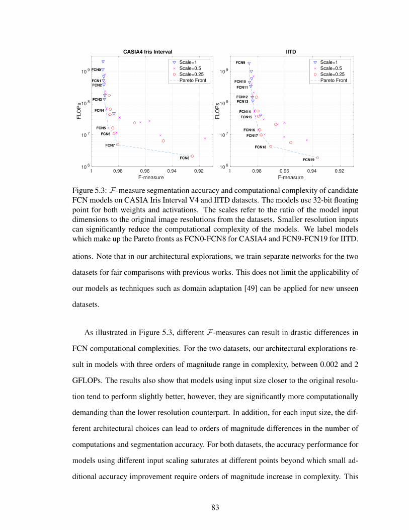
0.920.940.960.981

F-measure

106

107

108

109

FLO

Ps

CASIA4 Iris Interval

FCN8

FCN7

FCN6

FCN5

FCN4

FCN3

FCN2

FCN1

FCN0

Scale=1

Scale=0.5

Scale=0.25

Pareto Front

0.920.940.960.981

F-measure

106

107

108

109

FLO

Ps

IITD

FCN19

FCN18

FCN17

FCN16

FCN15

FCN14

FCN13

FCN12

FCN11

FCN10

FCN9 Scale=1

Scale=0.5

Scale=0.25

Pareto Front

Figure 5.3: F-measure segmentation accuracy and computational complexity of candidateFCN models on CASIA Iris Interval V4 and IITD datasets. The models use 32-bit floatingpoint for both weights and activations. The scales refer to the ratio of the model inputdimensions to the original image resolutions from the datasets. Smaller resolution inputscan significantly reduce the computational complexity of the models. We label modelswhich make up the Pareto fronts as FCN0-FCN8 for CASIA4 and FCN9-FCN19 for IITD.

ations. Note that in our architectural explorations, we train separate networks for the two

datasets for fair comparisons with previous works. This does not limit the applicability of

our models as techniques such as domain adaptation [49] can be applied for new unseen

datasets.

As illustrated in Figure 5.3, different F-measures can result in drastic differences in

FCN computational complexities. For the two datasets, our architectural explorations re-

sult in models with three orders of magnitude range in complexity, between 0.002 and 2

GFLOPs. The results also show that models using input size closer to the original resolu-

tion tend to perform slightly better, however, they are significantly more computationally

demanding than the lower resolution counterpart. In addition, for each input size, the dif-

ferent architectural choices can lead to orders of magnitude differences in the number of

computations and segmentation accuracy. For both datasets, the accuracy performance for

models using different input scaling saturates at different points beyond which small ad-

ditional accuracy improvement require orders of magnitude increase in complexity. This

83

Table 5.2: Segmentation Accuracy Comparison to Previous Works

DB Method R P Fµ σ µ σ µ σ

CA

SIA

4In

terv

al

GST [5] 85.19 18 89.91 7.37 86.16 11.53Osiris [70] 97.32 7.93 93.03 4.95 89.85 5.47

WAHET [95] 94.72 9.01 85.44 9.67 89.13 8.39CAHT [74] 97.68 4.56 82.89 9.95 89.27 6.67Masek [65] 88.46 11.52 89.00 6.31 88.30 7.99IrisSeg [30] 94.26 4.18 92.15 3.34 93.10 2.65

IDN [7] 97.10 2.12 98.10 1.07 97.58 0.99Our FCN0 99.41 0.40 98.93 0.75 99.17 0.40

IIT

D

GST [5] 90.06 16.65 85.86 10.46 86.60 11.87Osiris [70] 94.06 6.43 91.01 7.61 92.23 5.80

WAHET [95] 97.43 8.12 79.42 12.41 87.02 9.72CAHT [74] 96.80 11.20 78.87 13.25 86.28 11.39Masek [65] 82.23 18.74 90.45 11.85 85.30 15.39IrisSeg [30] 95.33 4.58 93.70 5.33 94.37 3.88

IDN [7] 98.00 1.56 97.16 1.40 97.56 1.04Our FCN9 98.92 0.87 98.33 1.13 98.62 0.65

saturation behavior is also observed when all scaling factors are combined.

To compare the efficiency and segmentation performance of our models to previous

works, we also evaluate each model using the full dataset. While several of our designs

outperform state-of-the-art segmentation accuracy on both datasets, we only report in Ta-

ble 5.2 our best performing models, which are FCN0 and FCN9 in Figure 5.3 for CASIA

Interval V4 and IITD respectively. The architectural descriptions for FCN0 and FCN9

and their respective computational complexities are given in Table 5.3. The segmenta-

tion accuracies of other works reported in the table are obtained from IrisSeg [30] and

IrisDenseNet (IDN) [7]. Previously, IrisSeg achieved better segmentation accuracy per-

formance in comparison to other none-FCN segmentation methods such as GST [5], Osiris

[70], Masek [65], WAHET [95], and CAHT [74]. This result was outperformed by FCN-

based segmentation method proposed by IDN from Arsalan et al. [7]. In comparison to

IDN model, which requires more than 100 GFLOPs per inference, both of our FCN ar-

chitectures need less than 2 GFLOPs as shown in Table 5.3, which is 50× more efficient.

84

Table 5.3: Descriptions of FCN architectures and their computational complexities(MFLOPs) which achieve top segmentation accuracy among all models explored in Figure5.3 for CASIA Interval V4 and IITD datasets. As in Table 5.1, each CONV layer is fol-lowed by Batch Normalization and ReLU, and TCONV is followed by ReLU. FS denotesthe filter size, and the skip connections are represented by the arrows.

CASIA Interval V4 (FCN0) IITD (FCN9)Type/FS/Stride Output Size MFLOPs Type/FS/Stride Output Size MFLOPs

Input/–/– 1×272×320 – Input/–/– 1×240×320 –CONV/3×3/1 12×272×320 18.8 CONV/3×3/1 16×240×320 22.1CONV/3×3/2 24×136×160 112.8 CONV/3×3/2 32×120×160 176.9CONV/3×3/1 24×136×160 225.6 CONV/3×3/1 32×120×160 353.9CONV/3×3/2 24×68×80 56.4 CONV/3×3/2 32×60×80 88.5CONV/3×3/1 24×68×80 56.4 CONV/3×3/1 32×60×80 88.5CONV/3×3/2 24×34×40 14.1 CONV/3×3/2 32×30×40 22.1CONV/3×3/1 24×34×40 14.1 CONV/3×3/1 32×30×40 22.1CONV/3×3/2 24×17×20 3.5 CONV/3×3/2 32×15×20 55.3CONV/3×3/1 48×17×20 7.1 CONV/3×3/1 64×15×20 110.6

TCONV/4×4/2 24×34×40 12.5 TCONV/4×4/2 32×30×40 19.7CONV/3×3/1 24×34×40 14.1 CONV/3×3/1 32×30×40 22.1

TCONV/4×4/2 24×68×80 25.1 TCONV/4×4/2 32×60×80 39.3CONV/3×3/1 24×68×80 56.4 CONV/3×3/1 32×60×80 88.5

TCONV/4×4/2 24×136×160 100.2 TCONV/4×4/2 32×120×160 157.3CONV/3×3/1 24×136×160 225.6 CONV/3×3/1 32×120×160 353.9

TCONV/4×4/2 24×272×320 200.5 TCONV/4×4/2 16×240×320 314.6CONV/1×1/1 2×272×320 4.2 CONV/1×1/1 2×240×320 4.9Classifier/–/– 1×272×320 – Classifier/–/– 1×240×320 –

Approx. Total 1148 Approx. Total 1941

This large difference in computational overhead can be attributed to the fact that our net-

work architectures are significantly shallower with far fewer number of feature maps per

layer. In addition, our models utilize few shortcut connections instead of the costly dense

connectivity.

5.3.3 Quantization to Dynamic Fixed-Point

As we demonstrated in Chapter 3, reducing the data precision in DNNs can significantly

lower the computational overheads of the models. With the Pareto front models identified

in Figure 5.3, we co-design their data precision such that they can be run using lower-

85

cost computational units on the targeted hardware platform. Since quantization is a time-

consuming process, we do not target other models which are not on the Pareto front.

We propose to quantize the models to dynamic fixed-point (DFP) for both the weights

and activations. More detailed explanations of the DFP representation can be found in

Chapter 3 Section 3.2. In this format, each layer in the FCN models is represented by

five hyperparameters, namely (wbw, abw, wfl, ain, aout), for bitwidths of the weights and

activations/feature maps, and fractional lengths of the weights, input feature maps, and

output feature maps respectively. We fix the bitwidths of both weights and activations of

all the layers to be 8 bits.

In order to determine the proper fractional lengths for the weights and feature maps of

each layer, we first perform profiling of the trained floating-point models. For the weights,

we select layer-wise fractional lengths such that no overflow exists during the quantization.

For the feature maps, the profiling is done by using a randomly selected subset of training

data to perform forward passes with the models. During this inference process, we record

the largest activation for each layer. Similar to the weights, we then select layer-wise

fractional lengths such that there is no overflow. With these hyperparameters in place, we

then quantize the floating models to DFP by employing the same procedure as described

in Section 3.4 of Chapter 3.

5.3.4 End-to-end FCN Models Evaluation

The combinations of different input scalings, varying architectural parameters allow for

robust Pareto fronts between segmentation accuracy and computational complexity for

both datasets as shown in Figure 5.3. These Pareto fronts would not be possible using any

single scaling factor. However, segmentation accuracy alone cannot reliably determine

the impact on the overall recognition performance as demonstrated by Hofbauer et al.

86

(a) Input image (b) Segmentation output

(e) Mask and CirclesOverlaid

(f) Normalized Iris

(g) Iris encoding (top)and mask (bottom)

(c) Rough limbic boundary estimate

(d) Fine-grained Fitting usingCircular Hough Transform

Figure 5.4: Processing pipeline for contour fitting, normalization and encoding.

[40]. In order to select the most efficient model without sacrificing overall recognition

performance, the candidate models need to be evaluated using the end-to-end processing

pipeline. Since each end-to-end evaluation is time-consuming, we select as candidates the

FCN models which form the Pareto front and their quantized versions for each dataset.

To compute the overall recognition performance, we first perform segmentation on

each input iris image using the floating point or quantized FCN model. Each output mask

is then passed through our proposed contour fitting algorithm, which produces the center

coordinates and radii of the pupil and limbic boundaries. This information is passed on

to the normalization step based on Daugman’s rubber sheet model [19], which converts

the iris region into a 16×256 pixel grid. A 1-D log Gabor filter is then used to extract

features from the grid producing a 16×256-bit encoding. A 16×256-bit mask grid is also

produced to identify useful and none-useful encoding bits. Next, we describe the details

of our proposed contour fitting routine.

Proposed Contour Fitting Algorithm: Daugman’s rubber sheet model achieves iris 2D

positional and size invariance due to a new coordinate system created by the center points

and radii of the iris and the pupil [19]. With FCN-based segmentation, each output mask

87

only identifies the pixels belonging to the iris and not the exact center coordinates or

radii of the iris and the pupil. In order to extract this information, we develop a contour

fitting routine as shown in Figure 5.4. Given a segmentation output mask, we first perform

a rough estimate of iris center point and radius. This is done by analyzing the largest

connected object in the image and computing its centroid, which is the rough iris center

point. The iris radius is then approximated by taking the mean of the object’s major and

minor axis lengths.

Using the approximated center point and radius, we perform a more fine-grained

boundary fitting using the Circular Hough Transform (CHT) for circles with similar radii

to the rough estimate. After obtaining the final iris radius (r) and center point (x, y), we

search for the pupil using CHT for circles with radius range in the range [0.1r 0.8r] and

whose center points are within a region of interest (ROI) around (x, y). We select this

radius range because biologically, the pupil radius can be anywhere between 0.1 and 0.8

of the iris radius [20]. The ROI allows for a less noisy and more computationally efficient

localization of the pupil boundary.

Note that, the Daugman normalization used in our current pipelines assumes circular

limbic and pupillary boundaries. This assumption may not be suitable for some datasets

such as those explored in [18] in which the recognition performance may be affected.

However, it is a useful first order approximation, which can be built upon to fit in those

cases.

88

5.4 Implementation of Iris Recognition Pipeline on Em-

bedded SoC

So far, the majority of work on iris recognition focuses mostly on algorithmic designs

such as segmentation and feature extraction. There exist only a few studies on the system

design and implementation aspect. Hashemi et al. [37] and Lopez et al. [63] implemented

full recognition pipelines on an embedded FPGA platform and showed that careful param-

eters optimization and hardware-software partitioning are required to achieve acceptable

runtime. For iris recognition with FCN-based segmentation, existing studies so far are

only concerned with achieving state-of-the-art segmentation accuracy without considera-

tions for computational costs of the proposed designs. As such, full system analysis and

implementation of these processing pipelines have not been demonstrated. In this section,

we provide analysis of the FCN-based iris recognition pipeline runtimes and bottlenecks

on an embedded FPGA SoC. We then realize our HW/SW co-design of the pipeline by

proposing a dynamic fixed-point hardware accelerator, which is able to achieve significant

speedup computations relative to the onboard CPU core. Additionally, we synthesized a

floating-point version of our accelerator for runtime and resource utilization comparisons.

5.4.1 Runtime Profiles for Iris Recognition Pipeline

As an initial step, we implement the iris recognition pipeline in software running on the

physical CPU core on the FPGA SoC. Our pipeline consists of four main modules, namely

segmentation, contour fitting, normalization, and encoding. The segmentation step can be

performed using different FCN models, which can lead to vastly different runtimes. On the

other hand, the runtimes for the remaining three components stay approximately constant

across different input images and FCN models. This is because the dimensions of the

89

FCN8 FCN7 FCN6 FCN5 FCN4 FCN3 FCN2 FCN1 FCN00

0.2

0.4

0.6

0.8

1

No

rma

lize

d R

un

tim

e

Segmentation Circle Fitting Normalization Encoding

Figure 5.5: FCN-based iris recognition pipeline runtime breakdown for floating-pointFCN0–FCN8 models from CASIA Interval V4 Pareto front in Figure 5.3. From left toright, the FCN models are arranged in increasing computational complexity. Results arebased on floating-point FCN models.

Table 5.4: Runtime profile for floating-point FCN inference using the onboard CPU.

Function Init Im2Col GEMM Activation (ReLU)

Percentage 1.31 10.58 80.77 7.34

input and output images for these three modules are constant.

With this setup, we profile the runtime of the different components in the pipeline,

which is shown in Figure 5.5. Here, we observe that the majority of the runtime is spent in

the segmentation stage. This is especially true for larger FCN models where segmentation

takes up more than 95% of the total runtime. Therefore, it is reasonable to focus our

efforts on accelerating the segmentation component of the pipeline, which is essentially

the inference process of the FCN model. To effectively speed up this operation, we explore

next the runtime profiles for FCN model components. While the profile shown here is for

floating-point FCN models here, similar behavior is observed for quantized models.

90

5.4.2 FCN Processing Components

In this work, our FCN models are implemented and trained using the Darknet framework

[75]. Each model consists of multiple layers with different computational requirements,

and each layer consists of multiple components as listed in Table 5.4. Here, the Init func-

tions is responsible for ensuring that the output matrices are properly initialized and ze-

roed out. Note that Batch Normalization (BN) layers are used in training, but they are not

shown here since the trained normalization parameters (µ, σ2, γ, β) can be folded into the

network parameters in inference as such:

w = γ · w/σ2

b = γ · (b− µ)/σ2 + β

where w and b are the trained weights and biases of the preceding convolution layer. With

this, the forward computation can be carried out using w and b without the BN layers.

The Im2Col function, as illustrated in Figure 5.6, is a standard operation which converts

the input images/feature maps into column format. With this, the convolution operations

can be carried out using a general matrix to matrix multiplication (GEMM) routine. For

transposed convolution layer, a similar operation named Col2Im is used to convert column

data to images instead. The GEMM unit is essentially responsible for the multiplication of

two matrices, the weights and input feature maps. The results in Table 5.4 show that the

GEMM unit is the most time consuming portion taking up more than 80% of the module

runtime. The remaining 20% is spent mostly on Im2Col and activation function, which is

the rectify linear unit in this case. Again, we observe similar runtime profiles for quantized

models.

The resources onboard the SoC allow for multiple choices for accelerating the pipeline

91

Patc

h1

Patc

h2

…

im2col

Patch1 Patch2 …

Input Image

Figure 5.6: Image to column operation for convolution layer.

including parallelization and vectorization using embedded CPU cores and custom hard-

ware accelerator on the programmable logic (PL) fabric. In comparison to the PL, par-

allelization, and vectorization on the CPU offer limited number of arithmetic processing

units; however, accelerators on the PL side can face challenges in the limited on-chip

buffer size and memory bandwidths. Thus, in order to efficiently utilize the available

hardware resources, we leave the control logic and memory-access intensive component,

Im2Col, in software and move computational intensive module, GEMM, to PL by synthe-

sizing a custom accelerator. For the activation function, we process it using the CPU core

in parallel to the accelerator unit. Next, we describe in details our accelerator architecture.

5.4.3 Hardware Accelerator Architecture

For FCN models, the GEMM operation is carried out in every layer between the weight

and input feature matrices. The dimensions of the two matrices can be represented by

a 3-tuple, (M, K, N), where the weight matrix is M × K, and the input features matrix

is K × N . The output feature matrix is then M × N . Between different layers of an

FCN model, (M, K, N) vary significantly depending on the sizes and number of the input

and output feature maps. Evidence of this can be observed in the network architecture

shown in Table 5.3 for CASIA Interval V4. In this architecture, after Im2Col operation,

the (M, K, N) dimensions would be (16, 9, 76800) for Layer 1, whereas for Layer 2, these

92

Application Processing Unit

Zyn

q

Programmable Logic

ARM CPUsFPUsNEON

L1 Cache

L2 C

ach

e &

Co

ntr

oll

er

Snoop Controller

OCM

DMA

AcceleratorACP

CentralInterconnect

GP Ports

I/O

ACP

ACP

ACP

Buffer A

Buffer B

Buffer C

GEM

M A

cce

lera

tor Processing Engine

Processing EngineCode Synthesized into Hardware

for (i = 0; i < M; ++i){for (j = 0; j < N; ++j){

Dtype sum = 0;for (k = 0; k < K; ++k){

sum += A[i][k]*B[k][j];}C[i][j] += sum;

}}

×

×

×

×

A[0]B[0]A[1]B[1]A[2]B[2]

A[n]B[n]

+

+

+

clk

Figure 5.7: Overall system integration and the hardware accelerator module for the GEMMunit. The code representing the operations of the hardware module is shown in the bottomleft, where A and B are the multiplicant and multiplier matrices, and C is the resultingoutput matrix. For DFP version of the accelerator, A and B are 8-bit, and C is 16-bit.A, B and C are all 32-bit floats for the floating-point version. The accelerator module isconnected to the Zynq Processor Unit via the Accelerator Coherency Port (ACP).

dimensions become (32, 144, 19200). Among FCN models which use different input

image scaling factors, these dimensional differences are even more drastic. As such, the

accelerator unit must be able to accommodate these dimensional variations and maximize

utilization across all the models explored.

Figure 5.7 shows the overall system integration and the architecture of the accelerator

core. For comparisons, we synthesized two versions of the accelerator, one with DFP

and one with floating-point datatype. We implement tiling buffers for the weights (Buffer

A), input features (Buffer B), and output features (Buffer C). The sizes of these buffers

are selected based on the greatest common divisor among the models. For the candidate

models in Figure 5.3, these turn out to be 8×9 for matrix A, 9×224 for B, and finally

8×224 for matrix C. Note that, since we do not target a specific model, the sizes for A,

B, and C may not be optimal for any specific architecture. In final system deployment,

93

ACP

ACP

ACP

Buffer A

Buffer B

Buffer CGEM

M A

ccel

erat

orProcessing EngineShift &

Saturate16-bit

8-bit

8-bit

16-bit8-bit

8-bit

8-bit

Figure 5.8: A closer look at the data paths of the buffers in the DFP accelerator unit.

such dimensions can be further optimized according to the chosen FCN model. We used

Vivado High-Level synthesis (HLS) to develop the accelerator connected via an AXI4-

Full interface to Accelerator Coherency Port (ACP). Here, we use the ARM CPUs as the

control unit which is responsible for preparing and feeding correct addresses in of the input

and output matrices as well as sending the start signal. Once this start signal is received,

the accelerator unit accesses the input matrices, performs computations and writes the

output matrix to the designated address in the DDR RAM.

The accelerator in Figure 5.7 utilizes nine parallel multipliers each of which is con-

nected to different banks of block RAM contain portions of input from matrices A and

B. This matrix partitioning helps improve the throughput of the design. The output of the

multipliers are then summed together using an adder tree consisting of 9 adders. If the out-

put is a partial sum, it is written to buffer C for accumulation until completion before being

written back to the DRAM. For the floating-point version, all the datapaths and buffers are

32-bit wide. For the DFP version, Figure 5.8 provides a closer look at the datapaths. Since

DFP representation may result in different radix-point location for the feature maps be-

tween different FCN layers, we need to shift the output results accordingly. Afterward,

the output feature maps are converted to 8-bit and saturated if necessary.

94

5.5 Experimental Results

In this section, we discuss the segmentation and recognition performance of our proposed

processing pipeline. We also report the runtime performance for the FPGA implementa-

tion and speedup achieved using our hardware accelerator.

5.5.1 Experimental Setup

All of our experiments are performed using two well-known and publicly available iris

datasets, the CASIA Interval V4 [2] and IITD [3]. Both datasets are captured using near-

infrared range sensors and reflect real-world deployment conditions. The ground truth

segmentation masks used in all of our experiments are obtained from IRISSEG-EP [41].

We use segmentation from Operator A for CASIA Interval V4 dataset. For FCN training

and deployment, we use the Darknet framework [75]. We fully implement our processing

pipeline on the ZedBoard with Xilinx Zynq 7020 FPGA SoC and 512 MB DDR3 memory.

The chip contains two ARM Cortex A9 cores and programmable logic fabric with 85K

logic cells and 4.9Mb block RAM. Our iris recognition flow is run inside an embedded

Linux operating system.

5.5.2 Recognition Performance Evaluations and Comparisons

As discussed in Section 5.3.4, segmentation accuracy alone is not a sufficient indicator

of the overall recognition performance. The true trade-off between FCN model computa-

tional complexity and recognition performance can only be analyzed using an end-to-end

flow. That is, each model must be evaluated based on performance metrics such as Equal

95

Error Rate (EER) and its receiver operating characteristics (ROC). Since end-to-end evalu-

ation on all explored models is extremely time-consuming, we select only the models from

the Pareto fronts from Figure 5.3, which represent the most efficient models across the seg-

mentation accuracy levels. The models on the Pareto fronts are labeled FCN0–FCN8 and

FCN9–FCN19 for CASIA Interval V4 and IITD datasets respectively. For each dataset,

the labels are in decreasing order of computational complexity as well as segmentation

accuracy.

To evaluate the recognition performance of each FCN model, we perform all possi-

ble combinations of intra-class, which are different instances of the same iris, and inter-

class matchings. For CASIA Interval V4, this results in approximately 9K intra-class and

6.9M inter-class comparisons. For IITD, approximately 4.8K intra-class and 5M inter-

class comparisons are performed. In each matching, the hamming distance (HD) for two

iris encodings {encodingA, endcodingB} with masks {maskA, maskB} is computed as

follows:

HD =||(encodingA⊗ encodingB) ∩maskA ∩maskB||

||maskA ∩maskB||.

The Hamming distance is computed for different degrees of rotation in the range [-35◦,

35◦] between the two masks. From this, the smallest Hamming distance is recorded.

Comparisons to Previous Works

In order to compare with previous works, we first evaluate the recognition performance

of the original floating-point versions of the FCN models from the Pareto fronts of the

two datasets. The resulting ROC curves are shown in Figure 5.9. Here, the ground truth

results are obtained by using the segmentation from IRISSEG-EP [41] along with the rest

of our flow, which includes contour fitting, normalization, and encoding. As evidenced

96

0 0.05 0.1 0.15 0.2 0.25 0.3 0.35

FAR

0

0.05

0.1

0.15

0.2

0.25

0.3

0.35

FR

R

ROC for IITD

Ground Truth

FCN9

FCN10

FCN11

FCN12

FCN13

FCN14

FCN15

FCN16

FCN17

FCN18

FCN19

0 0.05 0.1 0.15 0.2 0.25 0.3 0.35

FAR

0

0.05

0.1

0.15

0.2

0.25

0.3

0.35

FR

R

ROC for CASIA Interval V4

Ground Truth

FCN0

FCN1

FCN2

FCN3

FCN4

FCN5

FCN6

FCN7

FCN8

Figure 5.9: Receiver Operating Characteristic (ROC) curves of FCN-based iris recognitionpipelines with ground truth segmentation and different floating-point FCNs models forCASIA Interval V4 and IITD datasets. In the legend of each dataset, the FCN models arearranged in increasing FLOPs from bottom to top. The zoom-in axis range is [0 0.02] forboth x and y directions.

here, our best performing models achieve ROC close to the ground truth. The EER along

with the F-measure achieved for each model are reported in Table 5.5. We also provide

comparison to previous methods, CAHT [74] and IrisSeg [30]. We observe that the ground

truth EER for each dataset computed using our flow is slightly lower than that reported in

IrisSeg. While we cannot provide an exact explanation for this result without full access

to their experimental setup, we suspect that our contour fitting step might be the reason

for the difference since both of the studies use Daugman’s normalization and encoding

methods.

97

Table 5.5: Equal Error Rate (EER) and segmentation accuracy (F-measure) compari-son between previous approaches, our FCN-based pipeline and groundtruth (GT). In eachdataset, FCN models are floating-point based and arranged in increasing FLOPs and F-measure from top to bottom.

CASIA Interval V4 IITDApproach EER (%) F -measure GFLOPs Approach EER (%) F -measure GFLOPs

CAHT [74] 0.78 89.27 – CAHT [74] 0.68 86.28 –IrisSeg [30] 0.62 93.10 – IrisSeg [30] 0.50 94.37 –

FCN8 12.24 92.55 0.002 FCN19 10.42 93.65 0.002FCN7 9.29 98.07 0.005 FCN18 8.89 97.04 0.004FCN6 1.10 98.35 0.011 FCN17 8.86 97.75 0.010FCN5 0.94 98.75 0.016 FCN16 6.96 97.94 0.014FCN4 0.64 98.93 0.060 FCN15 1.13 98.15 0.038FCN3 0.50 99.06 0.132 FCN14 0.82 98.24 0.054FCN2 0.43 99.09 0.380 FCN13 0.50 98.35 0.117FCN1 0.42 99.14 0.513 FCN12 0.60 98.38 0.154FCN0 0.38 99.17 1.143 FCN11 0.41 98.50 0.335

FCN10 0.19 98.59 0.453FCN9 0.29 98.62 1.791

GT 0.31 – – GT 0.16 – –

The results in Table 5.5 show that several of our FCN models in each dataset out-

perform previous state-of-the-art EER results from IrisSeg [30]. For CASIA Interval V4,

FCN0–FCN3 outperform IrisSeg with FCN0 reducing the EER by almost half. For IITD

dataset, FCN9–FCN11 surpass the previous methods with FCN9 reducing EER by more

than half. However, it is interesting to note that some of our models achieve significantly

higher segmentation accuracy than both CAHT and IrisSeg, while at the same time, these

models underperform the previous methods recognition performance. This discrepancy

can be attributed to the nature of FCN-based segmentation, which does not strongly ac-

count for fine-grained pupil and limbic boundaries labeling. This problem can throw off

the contour fitting module in the next stage producing inaccurate center points and radii.

This highlights the necessity to evaluate FCN-based design using end-to-end flow rather

than segmentation accuracy alone. In future work, this problem may be remedied by as-

signing larger loss to boundary pixels in comparison to other pixels.

Another evidence for the necessity to perform end-to-end evaluation is between FCN9

and FCN10, where the model with more than 3× computational complexity and higher

segmentation accuracy performs worse in overall recognition performance. This observa-

98

Table 5.6: Equal Error Rate (EER) and segmentation accuracy (F-measure) comparisonbetween the groundtruth (GT), floating-point, and DFP FCN-based recognition pipelinesusing the IITD dataset.

Floating-Point DFPModel EER (%) F-measure EER (%) F-measureFCN13 0.50 98.35 0.46 97.23FCN12 0.60 98.38 0.68 96.49FCN11 0.41 98.50 0.22 97.24FCN10 0.19 98.59 0.23 96.97FCN9 0.29 98.62 0.37 97.14

GT 0.16 – – –

tion is also true for between FCN12 and FCN13. Figure 5.9 also verifies this observation

where the ROC curves for FCN10 and FCN13 fall below those of FCN9 and FCN12 re-

spectively.

Comparisons between DFP and Floating-Point

Table 5.6 shows the segmentation accuracy and end-to-end recognition rate comparisons

between our floating-point FCN-based pipeline and their DFP counter part. The DFP

version of each FCN model is obtained by analyzing and finetuning the trained floating-

point weights. From the results in the Table, it is evidenced that the quantization process

negatively impacts the segmentation accuracy of the models. However, in many cases,

the quantization, in fact, improves the overall recognition rates. For instance, for FCN11,

FCN13, FCN14, FCN15 and FCN16, the EER improves significantly after quantization to

DFP.

99

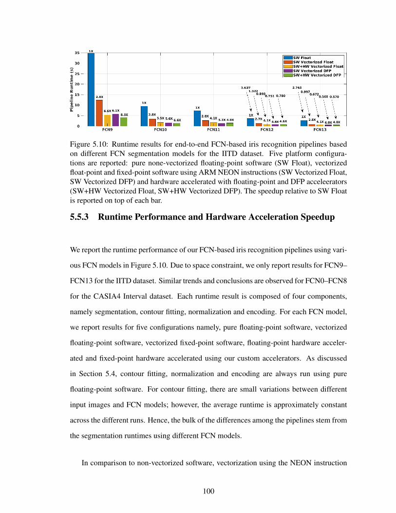
Figure 5.10: Runtime results for end-to-end FCN-based iris recognition pipelines basedon different FCN segmentation models for the IITD dataset. Five platform configura-tions are reported: pure none-vectorized floating-point software (SW Float), vectorizedfloat-point and fixed-point software using ARM NEON instructions (SW Vectorized Float,SW Vectorized DFP) and hardware accelerated with floating-point and DFP acceleerators(SW+HW Vectorized Float, SW+HW Vectorized DFP). The speedup relative to SW Floatis reported on top of each bar.

5.5.3 Runtime Performance and Hardware Acceleration Speedup

We report the runtime performance of our FCN-based iris recognition pipelines using vari-

ous FCN models in Figure 5.10. Due to space constraint, we only report results for FCN9–

FCN13 for the IITD dataset. Similar trends and conclusions are observed for FCN0–FCN8

for the CASIA4 Interval dataset. Each runtime result is composed of four components,

namely segmentation, contour fitting, normalization and encoding. For each FCN model,

we report results for five configurations namely, pure floating-point software, vectorized

floating-point software, vectorized fixed-point software, floating-point hardware acceler-

ated and fixed-point hardware accelerated using our custom accelerators. As discussed

in Section 5.4, contour fitting, normalization and encoding are always run using pure

floating-point software. For contour fitting, there are small variations between different

input images and FCN models; however, the average runtime is approximately constant

across the different runs. Hence, the bulk of the differences among the pipelines stem from

the segmentation runtimes using different FCN models.

In comparison to non-vectorized software, vectorization using the NEON instruction

100

Table 5.7: Utilization of FPGA Resources for Look-up Tables (LUT), LUT as memory(LUTRAM), Flip-Flop Registers, Block RAM (BRAM), Digital Signal Processing units(DSP), and Global Clock Buffers (BUFG).

LUT LUTRAM Flip-Flop BRAM DSP BUFGFloating Point 15% 3% 9% 5% 21% 3%

DFP 13% 2% 7% 5% 5% 3%

allows between 2.4× to 2.8× speedup. Software-based vectorized DFP outperforms vec-

torized floating-point in all cases. This is due to the smaller data movement needed by

DFP. In addition, vectorized DFP can use integer Arithmetic Logic Unit (ALU), which

has lower latency than floating-point ALU. Using our floating-point accelerator design,

we achieve between 2.4× and 6.6× speedup compared to pure non-vectorized software.

The DFP accelerator provides the best speedup for larger models, however, vectorized

DFP software outperforms other configurations for smaller models. This is due to the

larger cache inside the CPU core which allows for minimal DDR access. Overall, we ob-

serve that higher speedup is realized for larger FCN models since the fraction of runtime

spent in segmentation far exceeds that of other components. Additionally, the amount of

time spent in GEMM operations are also larger for larger models.

The resource utilization of our accelerators is reported in Table 5.7, and the floorplans

of the designs are shown in Figure 5.11. As discussed earlier, since our target models vary

significantly in architecture and computational requirement, we implement the accelera-

tors using only the greatest common divisor among them, which explains the low resource

utilization. However, with this design, we demonstrate that significant speedup can be

achieved while only utilizing a fraction of the available resource. Once a specific model is

chosen, a potentially larger speedup can be achieved by optimizing the accelerator design

and parameters.

As expected, we observe that overall the floating-point accelerator consumes more re-

101

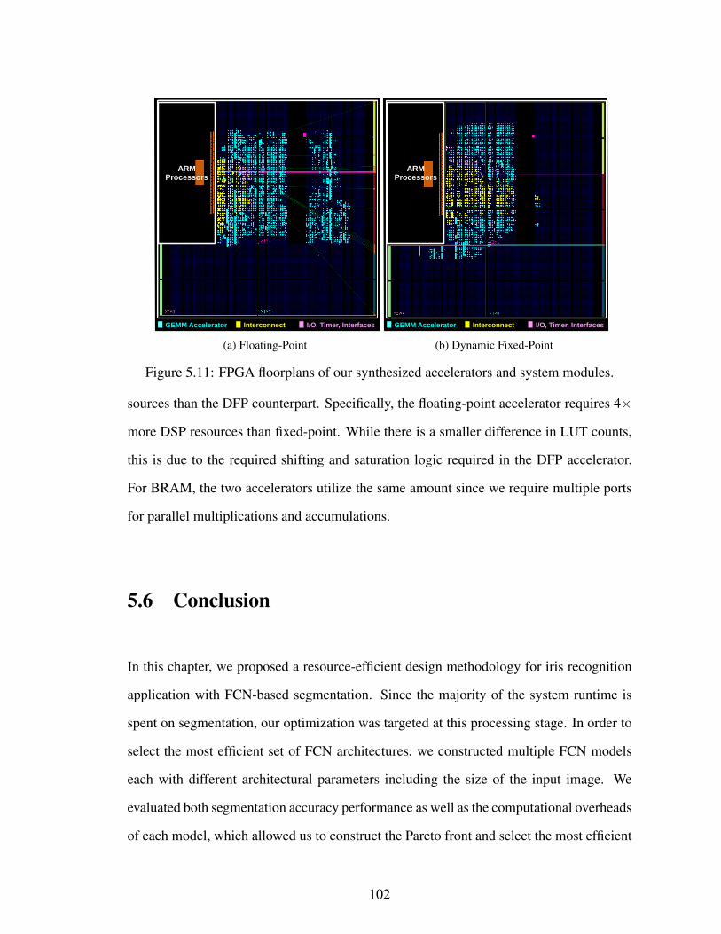
ARMProcessors

GEMM Accelerator Interconnect I/O, Timer, Interfaces

(a) Floating-Point

ARMProcessors

GEMM Accelerator Interconnect I/O, Timer, InterfacesDFP8x9 * 9x224

(b) Dynamic Fixed-Point

Figure 5.11: FPGA floorplans of our synthesized accelerators and system modules.

sources than the DFP counterpart. Specifically, the floating-point accelerator requires 4×

more DSP resources than fixed-point. While there is a smaller difference in LUT counts,

this is due to the required shifting and saturation logic required in the DFP accelerator.

For BRAM, the two accelerators utilize the same amount since we require multiple ports

for parallel multiplications and accumulations.

5.6 Conclusion

In this chapter, we proposed a resource-efficient design methodology for iris recognition

application with FCN-based segmentation. Since the majority of the system runtime is

spent on segmentation, our optimization was targeted at this processing stage. In order to

select the most efficient set of FCN architectures, we constructed multiple FCN models

each with different architectural parameters including the size of the input image. We

evaluated both segmentation accuracy performance as well as the computational overheads

of each model, which allowed us to construct the Pareto front and select the most efficient

102

set of models. Incorporating each model from the Pareto front into an end-to-end flow,

we evaluated their true recognition performance. Compared to FCN architectures from

previous works, our models set new state-of-the-art segmentation accuracy while being

being 50× more resource efficient. Furthermore, the recognition rates achieved using

our end-to-end pipelines outperform the results from previous works on the two datasets

evaluated. Through the evaluations of many FCN models in this design process, we also

showed that small EER increase of 0.7% can be traded off for an order-of-magnitude

reduction in overall computational complexities and runtime. Finally, we demonstrated

full implementation with a co-designed hardware accelerator for the processing flow on

an embedded FPGA SoC. In comparison to the onboard CPU, our accelerator is able to

achieve up to 8.3× speedup for the overall pipeline while using only a small fraction of

the available FPGA resources.

103

Chapter 6

Co-Design Techniques for

Chemical-based Neural Classifier

6.1 Introduction

As the daily amount of globally generated data is fast growing, relying on tradition von

Neumann-based digital logic for storage and processing may not be sufficient. Explo-

ration of alternative paradigms, which could potentially offer more flexibility in compu-

tation could pave the ways for massive growth in density and efficiency. In this Chapter,

we extend our work to an emerging computing paradigm for machine learning by intro-

ducing a novel methodology for a chemical-based single-layer neural network (NN). With

the billions of possible molecules each with a unique 3-dimensional structure, Chemistry

offers promising potentials for dense information storage and parallel processing which

may not be possible in traditional computer architectures. Inspired by these potentials,

we aim to develop a computational framework to concurrently process digital information

104

represented in chemical mixtures.

Our work, as presented here, has been published in [6]. The main contributions of this

work is as follows.

1. We propose a method to encode binary data into mixtures of chemical compounds.

Our technique allows multiple bits to be stored in parallel with multiple coexisting

chemicals. With this approach, we chemically encode several images of handwritten

digits from the MNIST database.

2. Using a robotic liquid handler, we perform volumetric multiply-accumulate opera-

tions for the single-layer NN on the parallelized chemical datasets. The results of the

computations are read and verified using a high-performance liquid chromatography

(HPLC).

3. In order to capture the robustness of this computing paradigm, we perform simu-

lations with various levels of uncertainties introduced. In addition, we verify this

robustness by carrying out chemical classifications with a larger set of binary vec-

tors.

The organization of this chapter is as follows. In Section 6.2, we discuss our methods

for chemical encoding, computation, and readout. A description of the system we devel-

oped to perform these functions is given in Section 6.3. In Section 6.4, we demonstrate

the simulations as well as experiments for classifications of several MNIST images and

Boolean test vectors. Section 5.6 summarizes the main conclusions of this chapter.

105

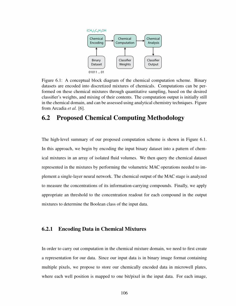
Binary

Dataset

Chemical

Encoding

Chemical

Computation

Weights

Chemical

Analysis

Output

(CH3)2C6H3OH

01011 ... 01

Figure 6.1: A conceptual block diagram of the chemical computation scheme. Binarydatasets are encoded into discretized mixtures of chemicals. Computations can be per-formed on these chemical mixtures through quantitative sampling, based on the desiredclassifier’s weights, and mixing of their contents. The computation output is initially stillin the chemical domain, and can be assessed using analytical chemistry techniques. Figurefrom Arcadia et al. [6].

6.2 Proposed Chemical Computing Methodology

The high-level summary of our proposed computation scheme is shown in Figure 6.1.

In this approach, we begin by encoding the input binary dataset into a pattern of chem-

ical mixtures in an array of isolated fluid volumes. We then query the chemical dataset

represented in the mixtures by performing the volumetric MAC operations needed to im-

plement a single-layer neural network. The chemical output of the MAC stage is analyzed

to measure the concentrations of its information-carrying compounds. Finally, we apply

appropriate an threshold to the concentration readout for each compound in the output

mixtures to determine the Boolean class of the input data.

6.2.1 Encoding Data in Chemical Mixtures

In order to carry out computation in the chemical mixture domain, we need to first create

a representation for our data. Since our input data is in binary image format containing

multiple pixels, we propose to store our chemically encoded data in microwell plates,

where each well position is mapped to one bit/pixel in the input data. For each image,

106

0 000 000 0

0000 0000 0000 0000 0000 00000000 01111 001111 00000000 001111 001111 00000000 001111 001111 00000000 01111 001111 00000000 01111

0000 00001111 11111111 11110000 00000000 0000 01111 00000000 0000 0000 0000 0000 0000

. . .0 0 0 0 0 00 0 0 00 0 0 00 0 0 00 0 0 00 0

1 11 11 11 11 1 0 00 0 0 0 0 0

image 1

analyte 1

0 0 0 0 0 00 0 00 0 0 0 00 0 0 00 0 0 00

1 1 111 11 11 1 1 1 00 0 0 0 0 0

image 2

analyte 2

1 11 1 1 11 1 1 11 11 1

0 0 0 0 0 00 0 0 00 00 00 0 0 00 0 0 00 0 0 0 0 0

image M

analyte M M analytes

M imagesspatially

overlay

Figure 6.2: Data is stored in isolated wells containing quantitative chemical mixtures.The concentrations of these chemicals reflect the values of the binary input data. Eachbit address in the input data is assigned to one grid location on a microplate, while thevalue of each bit is encoded in the concentration of a particular chemical compound at thatposition. Multiple datasets can be simultaneously stored in the same fluid containers byusing multiple distinct chemicals. Figure from Arcadia et al. [6].

we designate a specific chemical compound, which is used to encode its pixels. The pixel

intensity is represented using a high concentration (‘1’) or low concentration (‘0’) of the

designated chemical.

In order to enable parallel data storage and processing, we take advantage of the diver-

sity and uniqueness of different chemical compounds and overlay (concurrently encode)

multiple pixels from various input images in the datasets using the same set of wells in

the microplate. Figure 6.2 depicts this multiple input storage format for M binary image

inputs. Here, we take M binary images and realize all pixels with the same position in a

single well, by assigning a unique chemical species to each image.

In order to construct the parallelized data format shown in Figure 6.2, data in this

parallel format, we need to obtain a set of compatible chemical compounds. For a set

of chemical compounds to be considered compatible, they must satisfy a few criteria as

discussed below.

1. All the chemical compounds must be miscible in the chosen solvent.

2. The compounds must be stable, relatively inert, and not react with one another.

3. The chemicals must be compatible with analytical chemistry tools that can quantify

107

Table 6.1: Computational cost of classifying M binary inputs, each containing N bits, ina traditional versus volumetric neuron

Operations Scalar SingleCore Silicon

Parallel ChemicalMixtures

Additions M ·N − 1N

Multiplications M ·N

Total 2·M ·N − 1 N

their concentrations.

As demonstrated in Figure 6.2, the potential advantages of performing computation

with chemical mixtures stem from the ability for many datasets to coexist in parallel. For

instance, in the case of overlaid chemical images, any operation on a single well will

simultaneously be applied to the corresponding pixel in all images. As such, this encoding

scheme has the potential to support massively parallel storage and computation. Table 6.1

shows a comparison of the number of operations required for a neuron with a traditional

computer versus the proposed mixture-based technique. The number of operations needed

to be performed with chemical mixtures scales only with the number of input features and

is independent of the number of input instances.

6.2.2 Computing with Chemical Mixtures

Figure 6.3 illustrates the computational scheme for the proposed chemical mixture based

single-layer neural networks. The weights (wi ∈ [−1, 1]) are scaled to correspond to a

maximum volume Vo, which is chosen based on the available volume in the data wells.

Since we can only transfer positive liquid volumes, we pool wells with positive and nega-

108

mC+m-C–

0 000 000 0

0000 0000 0000 0000 0000 00000000 01111 001111 00000000 001111 001111 00000000 001111 001111 00000000 01111 001111 00000000 01111

0000 00001111 11111111 11110000 00000000 0000 01111 00000000 0000 0000 0000 0000 0000M analytes

M images

wi > 0wi < 0

0.4 0.6 0.5 0.9 0.8 0.81.0 0.3 0.7 0.6 0.5 0.70.4 0.0 0.8 0.5 0.2 0.70.7 0.4 0.0 0.4 0.9 0.60.1 0.3 0.3 0.8 0.4 0.80.7 0.3 0.7 0.9 0.9 0.70.8 0.1 1.0 0.5 0.5 0.4

weights

volumes

zyes nomatch mismatch

xi |wi|

timeabsorb

ance 1

2 . . .M

>0

∑∑

timeabsorb

ance

12

M. . .

negativepool positivepool

Figure 6.3: A schematic of the proposed chemical computation procedure, as implementedfor pattern classification. All spatially concurrent chemical datasets (x) are operated on inparallel by a single weight matrix (w), whose values are realized as volumetric fluid trans-fers. Since weights can be positive and negative (wi ∈ [−1, 1]), a pool for each polarity ismade. Each pool is analyzed by liquid chromatography to measure the concentrations ofeach analyte species. The differential concentration of each analyte is calculated in post-processing and used to determine the appropriate label for the input data. Figure fromArcadia et al. [6].

tive weights in two separate MAC operations.

The total volume that will be transferred from the ith well will be: Vi = |wi| · Vo.

As previously described, the scaling of the transfer volume represents a multiplication

and the pooling of volumes into a common well represents an addition. Since bits from

different datasets may be stored in the same well, these pooling operations allow for par-

allel multiply-accumulate operations on all concurrently stored datasets. There is zero

marginal computational cost to increasing parallelism, since, regardless of the complexity

of the chemical mixtures, we only need to perform the pooling transfers once.

109

Next, we show that the system in Figure 6.3 realizes the single-layer neural network

classifier. According to the conservation of mass, if a mixture of N sources, each contain-

ing a concentration Ci of a certain chemical, is formed by transferring a volume Vi from

each source to a common destination, then the final concentration will be given as:

Cf =N∑i=1

ViVf· Ci (6.1)

where Vi · Ci is the total mass of the chemical added to the destination and Vf is the

final total volume in the destination. We can then work backwards from the output of the

system. We can write the output for the data represented by molecular species m as:

zm = ∆Cm = C+m − C−m (6.2)

where C+m and C−m are the concentrations of species m in the positive and negative weight

pools, respectively. According to Equation 6.1 the concentration of molecule m at the

output of each MAC can be expressed as:

C+m =

N∑i=1wi>0

ViV +p

· Cmi =N∑i=1wi>0

|wi| · VoV +p

· Cmi (6.3)

and similarly:

C−m =N∑i=1wi<0

|wi| · VoV −p

· Cmi (6.4)

110

where V +p and V −P are the total volumes in each pool, i is the index of the data well, Vi =

|wi| ·Vo is the weighted volume transferred from the ith well, and Cmi is the concentration

of molecule m in the ith well. We can then expand Equation 6.2 as:

zm =N∑i=1wi>0

|wi| · VoV +p

· Cmi −N∑i=1wi<0

|wi| · VoV −p

· Cmi (6.5)

As long as the the pooled volumes are intentionally set to be equal after weighted pooling

(V +p = V −p = Vp), by appropriately adding pure solvent, we can collect the summations

as:

zm =N∑i=1

wi · VoVp

· Cmi =N∑i=1

wi · xmi (6.6)

where our features have been defined to be the scaled data concentrations: xmi = VoVp·Cmi.

This yields the original form of the pre-classification output that we sought to generate.

6.2.3 Reading the Results of Chemical Mixture Computations

To verify the output of the computations, we need to determine the amount of each compo-

nent present in the liquid samples. For this purpose, we chose to employ high-performance

liquid chromatography (HPLC). HPLC is a technique commonly used in analytical chem-

istry for separation, identification, and quantification of components in a mixture [52]. The

output from the HPLC is an absorbance time series, known as a chromatogram, which can

be used to infer the identity and concentration of the analytes in the solution. More details

regarding HPLC is available in our work [6].

111

Fluid HandlerDesktop Computer

Data Well Plate

SolventAnalytes

1 2 3

Weighted PoolsHPLC Unit

xi

|wi|

send instructionsfor liquid handling

writechemicaldata

xi|wi|∑i=1

N

read resultingconcentrations

volumetric multiply &accumulate

take computationresult to be analyzed

simulate &train weights&mC+ mC–

Figure 6.4: An overview of the experimental setup and data flow used for these exper-iments. Weight matrices were trained in simulation and then converted, along with testdata, into sequences of pipetting instructions for a robotic liquid handler. Analytes weredispensed into a 384-well microplate to form the chemical dataset and then collected involume fractions corresponding to the classifier weight matrix. The outputs were analyzedby HPLC to produce class labels. Figure from Arcadia et al. [6].

6.3 System Development

6.3.1 Experimental Setup

A diagram of our experimental setup and procedural workflow is shown in Figure 6.4.

Binary input data and classifier weights are first trained through simulations on a desktop

computer, in a Python environment. Prior to chemically encoding the input data, concen-

trated stock solutions are prepared of each analyte. The description and choice of analytes

are described in our work [6]. To write the chemical data to a 384-well plate, the binary

112

datasets are converted to pipetting instructions for a fluid handling robot. For each input

data bit whose value is ‘1’, the robot is instructed to transfer 20µL of the corresponding

analyte to the appropriate well. If the input data is ‘0’, it transfers 20µL of solvent in-

stead. After the chemical datasets are created, the classifier weights are converted into

additional pipetting instructions which the robot uses to perform the weighted-summation

operations, placing the pooled outputs into an empty well plate. The pooling operation

separates the source wells into two groups, those with corresponding positive weights and

those with negative ones. The positive and negative weights are two different destination

wells. Once the positive and negative weight pools are generated, each output is analyzed

using HPLC. The analytes representing each dataset exit the instrument at different times,

allowing separate estimations of the output concentration of each component. For each

analyte, the differential concentration (∆Cm) is calculated on a computer. If it is greater

than zero, then the data contained in the well plate is classified as a match; otherwise, the

data is classified as a mismatch.

6.4 Experiments & Results

For our first experimental demonstration, we used images derived from the well-known

MNIST database of handwritten digits [58]. The original images were grayscale at 28×28

pixel resolution, but for these experiments, we binarized and resized the images to 16×16.

We trained three one-versus-all classifiers on a computer a priori for three foreground

classes, representing the digits ‘0’, ‘1’, and ‘2’. Each classifier was trained using 100

foreground class images and 100 background class images which were randomly selected

from the MNIST training set. For example, the classifier with the digit ‘0’ foreground

class was trained using 100 images of the digit ‘0’ and 100 images of other digits ‘1’

through ‘9’.

113

6.4.1 Robustness Simulation

In this methodology, several sources of experimental variability which could affect the

exact output concentrations and measurements of the mixtures were expected. First, in

the data creation process, the actual pipetting volume for each transfer may deviate from

the target volume, which would vary the actual concentrations between different wells.

For instance, two wells whose corresponding pixel value are both ‘1’ could in fact contain

different concentrations of their corresponding analyte. Similarly, this pipetting inconsis-

tencies could also affect the actual volumes transferred in the weighted sum operations,

which would cause concentration variations in the pooled output. Another source of error

could stem from the HPLC, which was used in concentration reading of the output pools.

In order to capture these sources of uncertainties, we performed simulation of the neu-

ral network classifications with varying level uncertainties introduced prior to carrying out

the experiments. Here, we used the trained weights from the model with ‘0’ as the fore-

ground class. Our test set, disjoint from the training set, included 95 randomly selected im-

ages, 47 images of ‘0’ and 48 images of other digits. The results from the simulations are

shown in Figure 6.5. First, Figure 6.5a shows the classification error introduced from the

varying uncertainties in image creation portion while assuming the volumetric multiply-

accumulate and HPLC readings were assumed to be exact. Here, the left-most data point

shows the ground truth classification error rate, where no uncertainty was presented. As

the volume uncertainties increase, we observed that the mean and standard deviation of the

classification errors start to increase. For Figure 6.5b, we fixed the volume uncertainty for

image creation at 0.05 while varying the uncertainties in the multiply-accumulate pooling

volumes. We assumed the HPLC concentration reading to be exact. In both figures, we

can see that the neural network is quite robust to uncertainties up to approximately 7%,

which is quite larger than those from high-quality liquid handling equipment.

114

0.0 2.5 5.0 7.5 10.0 12.5 15.0 17.5 20.0Percentage volume uncertainty in image creation

0.070

0.075

0.080

0.085

0.090

0.095

Clas

sifica

tion Error R

ate

(a)

0.0 2.5 5.0 7.5 10.0 12.5 15.0 17.5 20.0Percentage volume uncertainty in pooling volume

0.070

0.075

0.080

0.085

0.090

0.095

Classif

icatio

n Error R

ate

(b)

Figure 6.5: Single-layer neural network classification simulation results. Figure (a) showsthe classification error introduced from the varying uncertainties in image creation portionwhile assuming the volumetric multiply-accumulate and HPLC readings are assumed tobe exact. For Figure (b), the volume uncertainty for image creation was fixed at 0.05while varying the uncertainties in the multiply-accumulate pooling volumes. The HPLCconcentration reading was assumed to be exact. For each data point in both figures, themean and standard deviation are computed from a trial of 100 runs.

6.4.2 MNIST Image Classification

In this section, we show the results from our image classification experiments using a

three-neuron, single-layer neural network. The color maps of the trained weight matrices

are shown in Figure 6.6.

We constructed a dataset of three overlaid MNIST images, consisting of two distinct

‘0’ images and one image of ‘1’. These images were mapped onto a well plate and encoded

with the three previously discussed analytes. The resulting microplate is shown in Figure

6.6, where the chemically encoded images are faintly visible due to the colors of the

analyte solutions (particularly analyte 3). We used the trained classifier to operate on

this chemical data, and the resulting MNIST classifications are shown in Figure 6.6. As

expected, the ‘0’ classifier correctly identified the two images with zeros, and the ‘1’

classifier correctly identified the image of a one. In total, all 9 of the MNIST neural

network outputs were correctly labeled. We note that while this model performed well,

115

the exact accuracy of the classifiers is not the main focus of this paper. Rather, our aim is

to reproduce the neural network operations using chemical computations.

yes noyes

yesno no

no no no

-1 0 +1

Stored Chemical Data

analyte 1 analyte 2 analyte 3Query

trainedweightsdigitclass

0

1

2

was there a match?(a)

yes noyes

yesno no

no no no

-1 0 +1

Stored Chemical Data

analyte 1 analyte 2 analyte 3Query

trainedweightsdigitclass

0

1

2

was there a match?

(b)

Figure 6.6: Chemical classification of MNIST handwritten digits. Three 16×16 (256-bit) binary images were chemically encoded, in parallel, on a 384-well plate. The overlaidchemical images were then classified by a three-neuron, single-layer neural network whichhad been previously trained to identify either digit ‘0’, ‘1’, or ‘2’. The results of thisexperiment are shown in a table format as class matches (zm > 0) or mismatches (zm < 0).All nine chemical classifier outputs were correct (3 true positives, 6 true negatives) (shownin (a)). A photograph of the microplate containing the chemical dataset of overlaid imagesis also shown in (b). Each well in the plate contains 60µL of liquid whose chemicalcomposition represents the values of one pixel across three images. Figure from Arcadiaet al. [6].

6.4.3 Performance Evaluation

Our chemical computation is not limited to images and is extensible to classifications of

any binary dataset. To evaluate the robustness of the computations, we performed a set

of experiments using smaller pseudo-random binary vectors. Sixteen 16-element weight

vectors (w ∈ [−1, 1]) were selected at random, as shown in Figure 6.7. For each w, we

chose three 16-bit data vectors, selected such that one vector is classified with large margin

116

ℓ# inputs

1

x1

w

x2

x3

0 0 0 1 0 0 0 0 0 0 1 1 0 0 0 1

0 0 1 0 0 0 0 1 0 0 0 1 0 0 1 0

0 1 0 1 0 0 1 0 0 1 0 0 0 0 0 1

1

1

0

2

x1

w

x2

x3

0 0 0 1 0 0 0 1 0 0 0 1 0 0 1 1

0 0 1 1 0 0 1 0 0 0 0 0 0 0 0 1

0 0 0 0 1 1 0 1 1 0 1 1 0 0 1 0

0

1

0

3

x1

w

x2

x3

0 0 0 1 0 0 0 1 0 0 0 0 0 0 1 1

0 0 1 0 0 0 0 1 0 0 0 0 0 0 1 1

0 1 0 1 0 1 1 0 0 0 1 1 0 0 0 0

1

0

1

4x1

w

x2

x3

0 0 0 0 0 0 0 1 0 0 0 1 0 0 1 1

0 0 0 1 0 0 1 1 0 0 0 0 0 0 0 1

0 0 1 1 0 0 0 0 0 1 1 1 0 1 1 0

0

0

1

5

x1

w

x2

x3

0 0 0 1 0 0 1 1 0 0 0 0 0 0 0 1

0 0 1 0 0 0 0 0 0 0 1 1 0 1 1 1

1 0 0 1 0 0 1 1 0 0 0 0 0 0 0 0

1

1

0

6

x1

w

x2

x3

0 0 0 1 0 0 0 0 0 0 0 1 0 0 1 1

0 0 0 1 0 0 0 1 0 0 1 0 0 0 0 1

0 1 1 1 0 0 1 0 0 1 0 0 0 0 1 0

0

0

1

7

x1

w

x2

x3

0 0 0 1 0 0 0 0 0 0 0 1 0 0 1 1

0 0 1 1 0 0 0 1 0 0 1 0 0 0 0 1

0 0 0 0 0 1 1 0 0 0 0 1 0 0 1 0

0

0

1

8

x1

w

x2

x3

0 0 0 1 0 0 0 0 0 0 0 1 0 0 1 1

0 0 0 0 0 0 0 0 0 0 1 1 0 1 0 1

0 0 0 1 0 0 0 1 0 1 0 0 0 0 1 0

0

1

0

ℓ# inputs

9

x1

w

x2

x3

0 0 0 0 0 0 0 1 0 0 0 1 0 0 1 1

0 0 0 1 0 0 0 0 0 0 1 1 0 0 1 0

0 0 0 0 0 1 0 1 0 0 1 0 0 0 0 1

1

1

0

10

x1

w

x2

x3

0 0 0 1 0 0 1 0 0 0 1 1 0 0 0 0

0 0 1 1 0 0 0 1 0 0 0 1 0 0 1 1

0 0 0 1 1 0 0 0 0 1 1 0 0 0 0 0

1

1

0

11

x1

w

x2

x3

0 0 0 1 0 0 0 1 0 0 0 1 0 0 1 0

0 0 0 1 0 0 0 1 0 0 1 1 0 0 0 1

0 1 0 0 0 0 1 0 0 1 0 1 0 1 1 0

0

0

1

12

x1

w

x2

x3

0 0 0 1 0 0 0 0 0 0 1 1 0 0 1 0

0 0 1 0 0 0 1 1 0 0 0 1 0 0 1 1

0 1 0 1 0 0 0 0 1 1 1 0 0 1 0 0

1

1

0

13

x1

w

x2

x3

0 0 0 1 0 0 0 1 0 0 0 1 0 0 0 1

0 0 0 0 0 0 1 0 0 0 0 1 0 0 1 1

0 1 1 1 0 0 0 0 0 0 1 0 0 0 0 0

0

0

1

14

x1

w

x2

x3

0 0 0 1 0 0 0 0 0 0 1 1 0 0 1 1

0 0 0 0 0 0 1 0 0 0 0 1 0 1 0 1

0 0 1 1 0 1 0 0 0 1 1 0 0 0 1 0

0

0

1

15

x1

w

x2

x3

0 0 0 0 0 0 0 1 0 0 0 1 0 0 1 1

0 0 0 1 0 0 0 0 0 0 1 1 0 0 1 0

0 1 0 0 0 0 0 1 1 0 0 1 0 0 0 1

0

1

0

16

x1

w

x2

x3

0 0 0 0 0 0 0 1 0 0 1 1 0 0 0 1

0 0 0 0 0 0 1 0 0 0 1 1 0 0 1 0

0 0 0 1 0 0 1 0 0 1 0 0 1 0 0 0

1

1

0

-1 -0.5 0 0.5 1 -1 -0.5 0 0.5 1

Figure 6.7: Validation experiments for chemical classifiers with pseudo-random data. Six-teen trials were performed. In each trial, three 16-bit data vectors (x1, x2, x3) were chem-ically encoded and classified according to a weight vector (w). The computed class label(`) is shown for each vector, along with a green check mark or red cross out to indicatewhether or not the chemical classifier identified it correctly. In total, 46 out of 48 vectorswere correctly classified (96% accurate with 2 false positives). Figure from Arcadia et al.[6].

as a mismatch (` = 0), one vector is easily classified as a match (` = 1), and one vector is

near the classifier’s boundary.

As described earlier, the classification output is robust to moderate experimental vari-

ations due to the uncertainties in volume transfers as we as the concentration readouts. In

total, the errors observed are in the range of 10% of the expected outputs. This naturally

has more significant impacts for data point lying closer to the decision boundaries of the

classifiers.

117

6.5 Conclusion

We have presented a scheme for implementing single-layer NN classification operations

using chemical mixtures. Binary input data is encoded in the chemical composition of an

array of liquid samples, and a robotic fluid handler is programmed to perform multiplica-

tions and additions as fractional volume transfers and pooling operations. The chemical

coding enables parallel computation and allows for increased information density. The re-

sult of the volumetric operations is represented in the concentration of chemicals in output

pools, which are analyzed using high-performance liquid chromatography. We used this

system for parallel classification of several 16×16 binary MNIST images of handwritten

digits, as well as a set of pseudo-random binary vectors. The method’s overall accuracy

was demonstrated, producing 55 correct classifications out of 57 tests.

118

Chapter 7

Summary of Dissertation and Possible

Future Directions

In this thesis, we proposed novel methodologies targeting resource-efficient design and ac-

celerations of Deep Neural Networks (DNNs) both at design-time and at runtime. We ex-

tensively evaluated the impacts of the proposed techniques using a variety of datasets. Our

accelerator designs were evaluated using both simulations and synthesis with industry-

strength standard cell libraries. Furthermore, we proposed an end-to-end iris recognition

flow with FCN-based segmentation where we applied the resource-efficient methodolo-

gies to optimize the processing pipeline. We fully implemented the flow on an embedded

FPGA platform and demonstrated significant resource and latency saving. Finally, we

showcased a promising direction in chemical-based computing by demonstrating a paral-

lelized classifications using a single-layer neural network (NN).

In this chapter, we provide a summary of the main contributions of this thesis and

discuss potential future extensions.

119

7.1 Summary of Results

In Chapter 3, we analyzed the numerical precisions and quantizations for DNN acceler-

ators. We evaluated a broad range of numerical approximations in terms of accuracy, as

well as design metrics such as area, power consumption, and energy requirements. We

studied floating-point arithmetic, different precisions of fixed-point arithmetic, quantiza-

tions of the weights to be of powers of two, and finally binary networks where the weights

are limited to one-bit values. In addition, we demonstrated a hardware design capable of

incorporating the dynamic fixed-point precision. We described the changes in the train-

ing procedure that are required to handle networks with lower precisions. To boost the

accuracy of low-precision networks, we have utilized ensemble processing. We evaluated

our designs and report the results using two well-known and challenging datasets, namely

CIFAR-10 and ImageNet, and design our networks based on well-studied architectures in

literature. Our DNN accelerators were able to achieve nearly 90% energy savings while

producing insignificant degradation of approximately 1% in accuracy performance. Fur-

thermore, we showed that this degradation can be fully compensated through the use of an

ensemble of just two quantized networks. With this ensemble, the accuracy of the quan-

tized models outperforms the floating-point networks by more than 1% for CIFAR-10 and

0.5% for ImageNet while still delivering energy savings of 80%.

Next in Chapter 4, we built on top of the design-time DNN hardware-software co-

design techniques by introducing two runtime trade-off strategies, which aim to lower the

latency of DNN deployment while maintaining minimal impact on accuracy performance.

First, in section 4, we proposed a dynamic configuration approach for DNNs in conjunc-

tion with a co-designed incremental training methodology. With this configuration, parts

of the DNN model can be dynamically shutdown at runtime to lower the computational

costs and latency. Using this approach, targeted accuracy performance can be achieved

120

while allowing for runtime configurable energy and delay budget. It also enables the DNN

to meet runtime constraints such as response time or power with a graceful trade-off in ac-

curacy. We show that our technique can be used to enable large energy saving with very

small accuracy reduction using three DNN benchmarks. We evaluate these savings using

our custom hardware design accelerator as well as Jetson TX1, an embedded GPU plat-

form. In comparison to the previous dynamic configuration technique, the methodology

introduced here requires significantly less memory and silicon real-estate.

Next, in section 4.2, we introduced a flexible processing strategy for DNN ensem-

bles, which allows conditional execution of the models in the ensemble for latency saving.

We evaluated the technique on ensembles of up to 8 models of well-known DNN archi-

tectures, AlexNet, and ResNet-50 with the ImageNet datasets. For both of the models

evaluated, flexible ensemble processing was able to retain the majority of the inference

accuracy compared to normal DNN ensembles while offering a significant saving in aver-

age latency. More specifically, on a platform with Intel Core i7-4790K and Titan Xp GPU,

we were able to reduce the average latency for an ensemble of 7 AlexNet models by close

to 2× while introducing a negligible accuracy loss of 0.1%. In the case of extremely tight

accuracy constraint, where no accuracy drop is tolerable, we can trade-off the latency sav-

ing by setting a very high score margin thresholds, which would be equivalent to normal

ensemble execution and leads to no accuracy loss.

In Chapter 5, we proposed a resource-efficient design methodology for iris recognition

application with FCN-based segmentation. Through our profiling of the overall processing

pipeline, we identified that the majority of the runtime is spent on the segmentation step,

which is the FCN model. Targeting this processing stage, we introduced an hardware-

software co-design methodology. First, we introduced a design space exploration for the

FCN architecture to select the most efficient set of models. The exploration was performed

through a grid search on several architectural parameters including the size of the input

121

image. For each architecture, we evaluated its segmentation accuracy performance as well

as the computational overheads of each FCN model. We then identified the most effi-

cient set of models, which form a Pareto front. Compared to the FCN architectures from

previous works, several of our models set new state-of-the-art segmentation accuracy on

two well-known datasets, which are CASIA Iris Interval V4 and IITD, while being 50×

more resource efficient. Furthermore, we evaluated the true recognition rate of each model

using the end-to-end pipelines and showed that the models outperformed the recognition

rate from previous works on the two datasets. Our architectural exploration in this de-

sign process showed that a small EER increase of 0.7% can be traded off for orders of

magnitude reduction in computational complexities and latency. With this set of mod-

els, we co-designed their datatype to dynamic fixed-point formats for friendly hardware

execution. Finally, we introduced an FPGA-based dynamic fixed-point accelerator and

demonstrated a full implementation of an accelerated processing flow on an embedded

FPGA SoC. We also synthesized a floating-point version of the accelerator for runtime

and resources comparisons. In comparison to the onboard CPU, our accelerator is able to

achieve up to 8.3× speedup for the overall pipeline while using only a small fraction of

the available FPGA resource.

In Chapter 6, we introduced a novel methodology for chemical-based single-layer NN,

which can operate on parallel datasets. We proposed a method to encode the binary data

into chemical mixtures and showed that multiple datasets can be stored in parallel us-

ing multiple coexisting chemicals. Using a programmable robotic liquid handler, we

performed sequences of volumetric multiply-accumulate operations on the parallelized

chemical datasets. We then utilized a high-performance liquid chromatography to read

and verify the output results from the chemical computations. Prior to carrying out the

experiments, we performed a simulation of the single-layer NN classifications with vary-

ing level uncertainties introduced. Through these simulations we observed that the net-

122

work is quite robust to uncertainties up to approximately 7%, which is quite larger than

those from high-quality liquid handling equipment. Our chemical-based single-layer NN

were able to successfully classify several binary, chemically-encoded images from the

MNIST handwritten digit database. Additionally, we further quantified the robustness of

our methodology by using a larger set of pseudo-random binary vector to perform the

classifications. With these experiments, we observed that the classification output is ro-

bust to moderate experimental uncertainties. While the demonstration was still at an early

stage, we consider this as a first step to building chemical systems, which can complement

electronic computing systems for applications in ultra-low-power systems and extreme

environments.

7.2 Potential Research Extensions

In this thesis, we explored various methodologies targeted at resource-efficient design

and accelerations of DNNs and their applications. We also introduced a chemical-based

computing domain. Based on the work presented here, several possible extensions can be

made as follows.

First, in regards to hardware-software co-design of DNNs, our optimization was tar-

geted the inference aspect of the models. A useful addition would be an evaluation of

the precisions required in the training phase, which would be helpful for online learning

deployment scenarios. Since our original publications, there have been many new, more

efficient types of architectures introduced such as depth-wise separable convolution [44].

Incorporating these new architectures into the co-design methodologies would offer ad-

ditional benefits and potential new insights. There have also been interesting works on

automatic exploration of DNNs architecture such as neural architecture search [104] to

123

achieve new state-of-the-art accuracy. Similar concepts could be used to automatically

explore architectures which are more amenable to quantization.

For the flexible inference strategies introduced in Chapter 4, while we demonstrated

a promising reduction in computational overheads and latency, a few extensions can be

made. First, similar to our hardware-software co-design work, the models evaluated so far

were restricted to convolutional neural networks (CNNs). A possible extension would be

to explore other kinds of models such as long-short term memory (LSTM) networks.

In our end-to-end iris recognition work, we introduced a methodology to optimize

the processing pipeline. We focused on the FCN portion since it was the most time-

consuming part. In addition to architectural exploration, quantization, and acceleration,

we plan to also include sparsification and introduce accelerator design, which is able to

process sparse, quantized FCN models. Such addition would decrease the data movement

significantly and introduce additional speedups. Expanding this methodology to other

biometric modalities such as 3D facial and gait recognition would also be a promising

future direction.

Finally, in regards to our work in chemical computation, the promise of this approach

as a viable alternative computing domain hinges upon its ability to scale up the parallelism

when operating on much larger datasets. Currently, our demonstrations are limited in

scale by several factors including the throughput of the robotic liquid handler, the read-

out operation, and the finite volume of chemical datasets. Moving forward, we anticipate

that improvements in robotics will allow us to increase the computational throughput by

several orders of magnitude. Such improvement would also allow for more efficient use

of the finite-volume chemical dataset.

124

Bibliography

[1] Cacti. http://www.hpl.hp.com/research/cacti/.

[2] Casia iris dataset, available online. http://biometrics.idealtest.org/

dbDetailForUser.do?id=4. Accessed on September 1, 2018.

[3] Iit delhi iris database, available online. http://web.iitd.ac.in/

˜biometrics/Database_Iris.htm. Accessed on September 1, 2018.

[4] Mohammed AM Abdullah, Satnam S Dlay, Wai L Woo, and Jonathon A Cham-

bers. Robust iris segmentation method based on a new active contour force with

a noncircular normalization. IEEE transactions on systems, man, and cybernetics:

Systems, 2017.

[5] Fernando Alonso-Fernandez and Josef Bigun. Iris boundaries segmentation using

the generalized structure tensor. a study on the effects of image degradation. In

IEEE International Conference on Biometrics: Theory, Applications and Systems

(BTAS), 2012.

[6] Christopher E Arcadia, Hokchhay Tann, Amanda Dombroski, Kady Ferguson,

Shui Ling Chen, Eunsuk Kim, Christopher Rose, Brenda M Rubenstein, Sherief

Reda, and Jacob K Rosenstein. Parallelized linear classification with volumetric

chemical perceptrons. In 2018 IEEE International Conference on Rebooting Com-

puting (ICRC), pages 1–9. IEEE, 2018.

125

[7] Muhammad Arsalan, Rizwan Ali Naqvi, Dong Seop Kim, Phong Ha Nguyen,

Muhammad Owais, and Kang Ryoung Park. Irisdensenet: Robust iris segmentation

using densely connected fully convolutional networks in the images by visible light

and near-infrared light camera sensors. Sensors, 18(5), 2018.

[8] Jimmy Ba and Rich Caruana. Do deep nets really need to be deep? In Advances in

neural information processing systems, pages 2654–2662, 2014.

[9] Vijay Badrinarayanan, Alex Kendall, and Roberto Cipolla. Segnet: A deep con-

volutional encoder-decoder architecture for image segmentation. arXiv preprint

arXiv:1511.00561, 2015.

[10] Leo Breiman. Bagging predictors. Machine learning, 24(2):123–140, 1996.

[11] Cristian Bucilua, Rich Caruana, and Alexandru Niculescu-Mizil. Model compres-

sion. In Proc. of ACM SIGKDD, 2006.

[12] Srihari Cadambi, Abhinandan Majumdar, Michela Becchi, Srimat Chakradhar, and

Hans Peter Graf. A programmable parallel accelerator for learning and classifica-

tion. In Proceedings of the 19th international conference on Parallel architectures

and compilation techniques, pages 273–284. ACM, 2010.

[13] Srimat Chakradhar, Murugan Sankaradas, Venkata Jakkula, and Srihari Cadambi.

A dynamically configurable coprocessor for convolutional neural networks. ACM

SIGARCH Computer Architecture News, 38(3):247–257, 2010.

[14] Liang-Chieh Chen, George Papandreou, Iasonas Kokkinos, Kevin Murphy, and

Alan L Yuille. Deeplab: Semantic image segmentation with deep convolutional

nets, atrous convolution, and fully connected crfs. IEEE transactions on pattern

analysis and machine intelligence, 2018.

126

[15] Tianshi Chen, Zidong Du, Ninghui Sun, Jia Wang, Chengyong Wu, Yunji Chen,

and Olivier Temam. Diannao: A small-footprint high-throughput accelerator for

ubiquitous machine-learning. In ACM Sigplan Notices, volume 49, pages 269–284.

ACM, 2014.

[16] Yu-Hsin Chen, Joel Emer, and Vivienne Sze. Eyeriss: A spatial architecture for

energy-efficient dataflow for convolutional neural networks. In ACM SIGARCH

Computer Architecture News, volume 44, pages 367–379. IEEE Press, 2016.

[17] Matthieu Courbariaux, Yoshua Bengio, and Jean-Pierre David. Low precision arith-

metic for deep learning. arXiv preprint arXiv:1412.7024, 2014.

[18] John Daugman. New methods in iris recognition. IEEE Transactions on Systems,

Man, and Cybernetics, Part B (Cybernetics), 2007.

[19] John Daugman. How iris recognition works. In The essential guide to image pro-

cessing, pages 715–739. Elsevier, 2009.

[20] John G Daugman. High confidence visual recognition of persons by a test of statisti-

cal independence. IEEE transactions on pattern analysis and machine intelligence,

15(11), 1993.

[21] Robert H Dennard, Fritz H Gaensslen, V Leo Rideout, Ernest Bassous, and Andre R

LeBlanc. Design of ion-implanted mosfet’s with very small physical dimensions.

IEEE Journal of Solid-State Circuits, 9(5):256–268, 1974.

[22] Kapil Dev and Sherief Reda. Scheduling challenges and opportunities in integrated

cpu+ gpu processors. In Proceedings of the 14th ACM/IEEE Symposium on Em-

bedded Systems for Real-Time Multimedia, pages 78–83. ACM, 2016.

127

[23] Kapil Dev, Xin Zhan, and Sherief Reda. Power-aware characterization and mapping

of workloads on cpu-gpu processors. In 2016 IEEE International Symposium on

Workload Characterization (IISWC), pages 1–2. IEEE, 2016.

[24] Thomas G Dietterich. Ensemble methods in machine learning. In International

workshop on multiple classifier systems, pages 1–15. Springer, 2000.

[25] Zidong Du, Avinash Lingamneni, Yunji Chen, Krishna V Palem, Olivier Temam,

and Chengyong Wu. Leveraging the error resilience of neural networks for design-

ing highly energy efficient accelerators. IEEE Transactions on Computer-Aided

Design of Integrated Circuits and Systems, 34(8):1223–1235, 2015.

[26] Clement Farabet, Berin Martini, Benoit Corda, Polina Akselrod, Eugenio Culur-

ciello, and Yann LeCun. Neuflow: A runtime reconfigurable dataflow processor for

vision. In CVPR Workshops, pages 109–116, 2011.

[27] Clement Farabet, Cyril Poulet, Jefferson Y Han, and Yann LeCun. Cnp: An fpga-

based processor for convolutional networks. In 2009 International Conference on

Field Programmable Logic and Applications, pages 32–37. IEEE, 2009.

[28] Clement Farabet, Cyril Poulet, and Yann LeCun. An fpga-based stream processor

for embedded real-time vision with convolutional networks. In 2009 IEEE 12th

International Conference on Computer Vision Workshops, ICCV Workshops, pages

878–885. IEEE, 2009.

[29] Abhishek Gangwar and Akanksha Joshi. Deepirisnet: Deep iris representation with

applications in iris recognition and cross-sensor iris recognition. In IEEE Interna-

tional Conference on Image Processing, 2016.

[30] Abhishek Gangwar, Akanksha Joshi, Ashutosh Singh, Fernando Alonso-

Fernandez, and Josef Bigun. Irisseg: A fast and robust iris segmentation framework

for non-ideal iris images. In IEEE International Conference on Biometrics, 2016.

128

[31] Vinayak Gokhale, Jonghoon Jin, Aysegul Dundar, Berin Martini, and Eugenio Cu-

lurciello. A 240 g-ops/s mobile coprocessor for deep neural networks. In Proceed-

ings of the IEEE Conference on Computer Vision and Pattern Recognition Work-

shops, pages 682–687, 2014.

[32] Ian Goodfellow, Yoshua Bengio, and Aaron Courville. Deep learning. MIT press,

2016.

[33] Suyog Gupta, Ankur Agrawal, Kailash Gopalakrishnan, and Pritish Narayanan.

Deep learning with limited numerical precision. In International Conference on

Machine Learning, pages 1737–1746, 2015.

[34] Philipp Gysel. Ristretto: Hardware-oriented approximation of convolutional neural

networks. arXiv preprint arXiv:1605.06402, 2016.

[35] Song Han, Xingyu Liu, Huizi Mao, Jing Pu, Ardavan Pedram, Mark A Horowitz,

and William J Dally. Eie: efficient inference engine on compressed deep neural

network. In 2016 ACM/IEEE 43rd Annual International Symposium on Computer

Architecture (ISCA), pages 243–254. IEEE, 2016.

[36] Soheil Hashemi, Nicholas Anthony, Hokchhay Tann, R Iris Bahar, and Sherief

Reda. Understanding the impact of precision quantization on the accuracy and

energy of neural networks. In Design, Automation & Test in Europe Conference &

Exhibition (DATE), 2017, pages 1474–1479. IEEE, 2017.

[37] Soheil Hashemi, Hokchhay Tann, Francesco Buttafuoco, and Sherief Reda. Ap-

proximate computing for biometric security systems: A case study on iris scanning.

In IEEE Design, Automation & Test in Europe Conference & Exhibition, 2018.

[38] Kaiming He, Xiangyu Zhang, Shaoqing Ren, and Jian Sun. Deep residual learning

for image recognition. In Proceedings of the IEEE conference on computer vision

and pattern recognition, pages 770–778, 2016.

129

[39] Geoffrey Hinton, Oriol Vinyals, and Jeff Dean. Distilling the knowledge in a neural

network. arXiv preprint arXiv:1503.02531, 2015.

[40] Heinz Hofbauer, Fernando Alonso-Fernandez, Josef Bigun, and Andreas Uhl. Ex-

perimental analysis regarding the influence of iris segmentation on the recognition

rate. IET Biometrics, 5(3), 2016.

[41] Heinz Hofbauer, Fernando Alonso-Fernandez, Peter Wild, Josef Bigun, and An-

dreas Uhl. A ground truth for iris segmentation. In IEEE International Conference

on Pattern Recognition, 2014.

[42] Eric Horvitz and Geoffrey Rutledge. Time-dependent utility and action under un-

certainty. In Uncertainty Proceedings 1991, pages 151–158. Elsevier, 1991.

[43] Eric J Horvitz. Reasoning about beliefs and actions under computational resource

constraints. arXiv preprint arXiv:1304.2759, 2013.

[44] Andrew G Howard, Menglong Zhu, Bo Chen, Dmitry Kalenichenko, Weijun

Wang, Tobias Weyand, Marco Andreetto, and Hartwig Adam. Mobilenets: Effi-

cient convolutional neural networks for mobile vision applications. arXiv preprint

arXiv:1704.04861, 2017.

[45] Itay Hubara, Matthieu Courbariaux, Daniel Soudry, Ran El-Yaniv, and Yoshua Ben-

gio. Binarized neural networks. In Advances in neural information processing

systems, pages 4107–4115, 2016.

[46] Kyuyeon Hwang and Wonyong Sung. Fixed-point feedforward deep neural network

design using weights+ 1, 0, and- 1. In 2014 IEEE SiPS, 2014.

[47] Forrest N Iandola, Song Han, Matthew W Moskewicz, Khalid Ashraf, William J

Dally, and Kurt Keutzer. Squeezenet: Alexnet-level accuracy with 50x fewer pa-

rameters and¡ 0.5 mb model size. arXiv preprint arXiv:1602.07360, 2016.

130

[48] Ehsaneddin Jalilian and Andreas Uhl. Iris segmentation using fully convolutional

encoder–decoder networks. In Deep Learning for Biometrics. Springer, 2017.

[49] Ehsaneddin Jalilian, Andreas Uhl, and Roland Kwitt. Domain adaptation for cnn

based iris segmentation. BIOSIG 2017, 2017.

[50] Yangqing Jia, Evan Shelhamer, Jeff Donahue, Sergey Karayev, Jonathan Long,

Ross Girshick, Sergio Guadarrama, and Trevor Darrell. Caffe: Convolutional archi-

tecture for fast feature embedding. In Proceedings of the 22nd ACM international

conference on Multimedia, pages 675–678. ACM, 2014.

[51] Norman P Jouppi, Cliff Young, Nishant Patil, David Patterson, Gaurav Agrawal,

Raminder Bajwa, Sarah Bates, Suresh Bhatia, Nan Boden, Al Borchers, et al. In-

datacenter performance analysis of a tensor processing unit. In 2017 ACM/IEEE

44th Annual International Symposium on Computer Architecture (ISCA), pages 1–

12. IEEE, 2017.

[52] Barry L Karger. HPLC: Early and recent perspectives. Journal of Chemical Edu-

cation, 74(1):45, 1997.

[53] Joo-Young Kim, Minsu Kim, Seungjin Lee, Jinwook Oh, Kwanho Kim, and Hoi-

Jun Yoo. A 201.4 gops 496 mw real-time multi-object recognition processor

with bio-inspired neural perception engine. IEEE Journal of Solid-State Circuits,

45(1):32–45, 2010.

[54] WK Kong and D Zhang. Accurate iris segmentation based on novel reflection and

eyelash detection model. In IEEE International Symposium on Intelligent Multime-

dia, Video and Speech Processing, 2001.

[55] Alex Krizhevsky and Geoffrey Hinton. Learning multiple layers of features from

tiny images. Technical report, Citeseer, 2009.

131

[56] Alex Krizhevsky, Ilya Sutskever, and Geoffrey E Hinton. Imagenet classification

with deep convolutional neural networks. In Advances in neural information pro-

cessing systems, pages 1097–1105, 2012.

[57] Andrew Lavin and Scott Gray. Fast algorithms for convolutional neural networks.

In Proceedings of the IEEE Conference on Computer Vision and Pattern Recogni-

tion, pages 4013–4021, 2016.

[58] Yann LeCun, Leon Bottou, Yoshua Bengio, Patrick Haffner, et al. Gradient-based

learning applied to document recognition. Proceedings of the IEEE, 86(11):2278–

2324, 1998.

[59] Zhouhan Lin, Matthieu Courbariaux, Roland Memisevic, and Yoshua Bengio. Neu-

ral networks with few multiplications. arXiv preprint arXiv:1510.03009, 2015.

[60] Baoyuan Liu, Min Wang, Hassan Foroosh, Marshall Tappen, and Marianna Pensky.

Sparse convolutional neural networks. In Proceedings of the IEEE Conference on

Computer Vision and Pattern Recognition, pages 806–814, 2015.

[61] Nianfeng Liu, Haiqing Li, Man Zhang, Jing Liu, Zhenan Sun, and Tieniu Tan. Ac-

curate iris segmentation in non-cooperative environments using fully convolutional

networks. In IEEE International Conference on Biometrics, 2016.

[62] Jonathan Long, Evan Shelhamer, and Trevor Darrell. Fully convolutional networks

for semantic segmentation. In Proceedings of the IEEE conference on computer

vision and pattern recognition, 2015.

[63] Mariano Lopez, John Daugman, and Enrique Canto. Hardware-software co-design

of an iris recognition algorithm. IET Information Security, 2011.

[64] Li Ma, Yunhong Wang, and Tieniu Tan. Iris recognition using circular symmetric

filters. In IEEE International Conference on Pattern Recognition, 2002.

132

[65] L Masek and P Kovesi. Matlab source code for a biometric identification system

based on iris patterns. The School of Computer Science and Software Engineering,

The University of Western Australia, 2003.

[66] Warren S McCulloch and Walter Pitts. A logical calculus of the ideas immanent in

nervous activity. The bulletin of mathematical biophysics, 5(4):115–133, 1943.

[67] Gordon E Moore et al. Cramming more components onto integrated circuits, 1965.

[68] Yuval Netzer, Tao Wang, Adam Coates, Alessandro Bissacco, Bo Wu, and An-

drew Y. Ng. Reading digits in natural images with unsupervised feature learning.

In NIPS Workshop on Deep Learning and Unsupervised Feature Learning 2011,

2011.

[69] Eunhyeok Park, Dongyoung Kim, Soobeom Kim, Yong-Deok Kim, Gunhee Kim,

Sungroh Yoon, and Sungjoo Yoo. Big/little deep neural network for ultra low

power inference. In Proceedings of the 10th International Conference on Hard-

ware/Software Codesign and System Synthesis, pages 124–132. IEEE Press, 2015.

[70] D Petrovska and A Mayoue. Description and documentation of the biosecure soft-

ware library. Project No IST-2002-507634-BioSecure, Deliverable, 2007.

[71] Ahmad Poursaberi and Babak N Araabi. A novel iris recognition system using mor-

phological edge detector and wavelet phase features. ICGST International Journal

on Graphics, Vision and Image Processing, 5(6):9–15, 2005.

[72] Hugo Proenca and Luıs A Alexandre. The nice. i: noisy iris challenge evaluation-

part i. In IEEE International Conference on Biometrics: Theory, Applications, and

Systems, 2007.

133

[73] Mohammad Rastegari, Vicente Ordonez, Joseph Redmon, and Ali Farhadi. Xnor-

net: Imagenet classification using binary convolutional neural networks. In Euro-

pean Conference on Computer Vision, pages 525–542. Springer, 2016.

[74] Christian Rathgeb, Andreas Uhl, and Peter Wild. Iris biometrics: from segmenta-

tion to template security, volume 59. Springer Science & Business Media, 2012.

[75] Joseph Redmon. Darknet: Open source neural networks in c. http://

pjreddie.com/darknet/, 2013–2016.

[76] C. J. Van Rijsbergen. Information Retrieval. Butterworth-Heinemann, 2nd edition,

1979.

[77] Olaf Ronneberger, Philipp Fischer, and Thomas Brox. U-net: Convolutional net-

works for biomedical image segmentation. In International Conference on Medical

image computing and computer-assisted intervention. Springer, 2015.

[78] Frank Rosenblatt. Principles of neurodynamics. perceptrons and the theory of brain

mechanisms. Technical report, Cornell Aeronautical Lab Inc Buffalo NY, 1961.

[79] Olga Russakovsky, Jia Deng, Hao Su, Jonathan Krause, Sanjeev Satheesh, Sean

Ma, Zhiheng Huang, Andrej Karpathy, Aditya Khosla, Michael Bernstein, et al.

Imagenet large scale visual recognition challenge. International journal of com-

puter vision, 115(3):211–252, 2015.

[80] Murugan Sankaradas, Venkata Jakkula, Srihari Cadambi, Srimat Chakradhar, Igor

Durdanovic, Eric Cosatto, and Hans Peter Graf. A massively parallel coprocessor

for convolutional neural networks. In 2009 20th IEEE International Conference

on Application-specific Systems, Architectures and Processors, pages 53–60. IEEE,

2009.

134

[81] Syed Shakib Sarwar, Swagath Venkataramani, Anand Raghunathan, and Kaushik

Roy. Multiplier-less artificial neurons exploiting error resiliency for energy-efficient

neural computing. In Proceedings of the 2016 Conference on Design, Automation

& Test in Europe, pages 145–150. EDA Consortium, 2016.

[82] Pierre Sermanet, Soumith Chintala, and Yann LeCun. Convolutional neu-

ral networks applied to house numbers digit classification. arXiv preprint

arXiv:1204.3968, 2012.

[83] Samir Shah and Arun Ross. Iris segmentation using geodesic active contours. IEEE

Transactions on Information Forensics and Security, 2009.

[84] Daniel Soudry, Itay Hubara, and Ron Meir. Expectation backpropagation:

Parameter-free training of multilayer neural networks with continuous or discrete

weights. In Proc. NIPS, pages 963–971, 2014.

[85] Jost Tobias Springenberg, Alexey Dosovitskiy, Thomas Brox, and Martin Ried-

miller. Striving for simplicity: The all convolutional net. arXiv preprint

arXiv:1412.6806, 2014.

[86] Ilya Sutskever, James Martens, George Dahl, and Geoffrey Hinton. On the impor-

tance of initialization and momentum in deep learning. In International conference

on machine learning, pages 1139–1147, 2013.

[87] Chuan Zhang Tang and Hon Keung Kwan. Multilayer feedforward neural net-

works with single powers-of-two weights. IEEE Transactions on Signal Process-

ing, 41(8):2724–2727, 1993.

[88] Hokchhay Tann, Soheil Hashemi, R Bahar, and Sherief Reda. Runtime config-

urable deep neural networks for energy-accuracy trade-off. In Proceedings of the

Eleventh IEEE/ACM/IFIP International Conference on Hardware/Software Code-

sign and System Synthesis, page 34. ACM, 2016.

135

[89] Hokchhay Tann, Soheil Hashemi, R Iris Bahar, and Sherief Reda. Hardware-

software codesign of accurate, multiplier-free deep neural networks. In Design Au-

tomation Conference (DAC), 2017 54th ACM/EDAC/IEEE, pages 1–6. IEEE, 2017.

[90] Hokchhay Tann, Soheil Hashemi, Francesco Buttafuoco, and Sherief Reda. Ap-

proximate computing for iris recognition systems. In Approximate Circuits, pages

331–348. Springer, 2019.

[91] Hokchhay Tann, Soheil Hashemi, and Sherief Reda. Flexible deep neural network

processing. arXiv preprint arXiv:1801.07353, 2018.

[92] Hokchhay Tann, Soheil Hashemi, and Sherief Reda. Lightweight deep neural net-

work accelerators using approximate sw/hw techniques. In Approximate Circuits,

pages 289–305. Springer, 2019.

[93] Olivier Temam. A defect-tolerant accelerator for emerging high-performance ap-

plications. In ACM SIGARCH Computer Architecture News, volume 40, pages

356–367. IEEE Computer Society, 2012.

[94] Christel-loic Tisse, Lionel Martin, Lionel Torres, Michel Robert, et al. Person iden-

tification technique using human iris recognition. In Proc. Vision Interface, volume

294. Citeseer, 2002.

[95] Andreas Uhl and Peter Wild. Weighted adaptive hough and ellipsopolar transforms

for real-time iris segmentation. In IEEE International Conference on Biometrics,

2012.

[96] Swagath Venkataramani, Ashish Ranjan, Kaushik Roy, and Anand Raghunathan.

Axnn: energy-efficient neuromorphic systems using approximate computing. In

Proceedings of the 2014 international symposium on Low power electronics and

design, pages 27–32. ACM, 2014.

136

[97] Richard P Wildes, Jane C Asmuth, Gilbert L Green, Stephen C Hsu, Raymond J

Kolczynski, James R Matey, and Sterling E McBride. A system for automated iris

recognition. In Proceedings of the IEEE Workshop on Applications of Computer

Vision, 1994.

[98] Guangzhu Xu and Zaifeng Zang. An efficient iris recognition system based on

intersecting cortical model neural network. International Journal of Cognitive In-

formatics and Natural Intelligence, 2008.

[99] Chen Zhang, Peng Li, Guangyu Sun, Yijin Guan, Bingjun Xiao, and Jason

Cong. Optimizing fpga-based accelerator design for deep convolutional neural

networks. In Proceedings of the 2015 ACM/SIGDA International Symposium on

Field-Programmable Gate Arrays, pages 161–170. ACM, 2015.

[100] Shijin Zhang, Zidong Du, Lei Zhang, Huiying Lan, Shaoli Liu, Ling Li, Qi Guo,

Tianshi Chen, and Yunji Chen. Cambricon-x: An accelerator for sparse neural

networks. In The 49th Annual IEEE/ACM International Symposium on Microarchi-

tecture, page 20. IEEE Press, 2016.

[101] Zijing Zhao and Kumar Ajay. An accurate iris segmentation framework under re-

laxed imaging constraints using total variation model. In IEEE International Con-

ference on Computer Vision, 2015.

[102] Zijing Zhao and Ajay Kumar. Towards more accurate iris recognition using deeply

learned spatially corresponding features. In Proceedings of the IEEE International

Conference on Computer Vision, 2017.

[103] Jun Zheng. Predicting software reliability with neural network ensembles. Expert

systems with applications, 36(2):2116–2122, 2009.

[104] Barret Zoph and Quoc V Le. Neural architecture search with reinforcement learn-

ing. arXiv preprint arXiv:1611.01578, 2016.

137