Hardware Implementation of Genetic Algorithms

Kevin Hsiue and Bryan Teague

6.375: Complex Digital Systems - Spring 2013

Abstract

Genetic algorithms are a powerful optimization technique that offers many degreesof freedom so that they can be tailored to a specific problem. In very complex problemsthis process is usually recursive so that the algorithm is tuned as a solution is convergedupon. Genetic algorithms can also benefit from a hardware implementation due to theirhighly parallel nature.

Unfortunately flexibility and hardware tend to be mutually exclusive in nature andas a result countless hours can be spent optimizing a genetic algorithm in hardware fora specific problem with little usable IP actually generated.

The goal of this project is to develop a framework in Bluespec and an initial set ofIP to demonstrate that a flexible hardware implementation of a genetic algorithm canbe designed. Architecture tuning will be done at compile-time using clearly definedparameters. The architecture will be demonstrated on a complex antenna beamformingproblem, which serves as an appropriate vehicle to fully display the capabilities ofgenetic algorithms.

Contents

1 Background 11.1 Genetic Algorithms . . . . . . . . . . . . . . . . . . . . . . . . . . . . . . . . . 11.2 Beam Forming . . . . . . . . . . . . . . . . . . . . . . . . . . . . . . . . . . . 1

2 Project Objective 3

3 High-Level Design 4

4 Test Plan 44.1 Python Testing Suite . . . . . . . . . . . . . . . . . . . . . . . . . . . . . . . . 44.2 Bluespec Simulation Testbench . . . . . . . . . . . . . . . . . . . . . . . . . . 5

5 Microarchitectural Description 55.1 Antenna Cost Module . . . . . . . . . . . . . . . . . . . . . . . . . . . . . . . 65.2 Natural Selection Module . . . . . . . . . . . . . . . . . . . . . . . . . . . . . 6

5.2.1 Find Max/Min . . . . . . . . . . . . . . . . . . . . . . . . . . . . . . . 75.2.2 Bubblesort . . . . . . . . . . . . . . . . . . . . . . . . . . . . . . . . . 75.2.3 Thresholding . . . . . . . . . . . . . . . . . . . . . . . . . . . . . . . . 7

5.3 Crossover Module . . . . . . . . . . . . . . . . . . . . . . . . . . . . . . . . . . 75.3.1 Top Two Selection . . . . . . . . . . . . . . . . . . . . . . . . . . . . . 85.3.2 Tournament Selection . . . . . . . . . . . . . . . . . . . . . . . . . . . 85.3.3 Mating . . . . . . . . . . . . . . . . . . . . . . . . . . . . . . . . . . . 8

5.4 Mutation Module . . . . . . . . . . . . . . . . . . . . . . . . . . . . . . . . . . 95.5 Genetic Algorithm Processor . . . . . . . . . . . . . . . . . . . . . . . . . . . 95.6 SceMi Layer Module . . . . . . . . . . . . . . . . . . . . . . . . . . . . . . . . 105.7 Test Bench . . . . . . . . . . . . . . . . . . . . . . . . . . . . . . . . . . . . . 10

6 Implementation Evaluation and Performance 116.1 Sequential Implementation . . . . . . . . . . . . . . . . . . . . . . . . . . . . . 116.2 Pipelined Implementation . . . . . . . . . . . . . . . . . . . . . . . . . . . . . 12

6.2.1 Cost Function Module . . . . . . . . . . . . . . . . . . . . . . . . . . . 136.2.2 Natural Selection Module . . . . . . . . . . . . . . . . . . . . . . . . . 146.2.3 Crossover Module . . . . . . . . . . . . . . . . . . . . . . . . . . . . . 156.2.4 Mutation Module . . . . . . . . . . . . . . . . . . . . . . . . . . . . . . 16

7 Design Exploration 16

1 Background

1.1 Genetic Algorithms

Genetic algorithms represent a powerful brute-force optimization method that has provenuseful in a number of applications including airframe design, antenna design, high frequencycircuit design, and microfluidics. The approach is particularly useful in nonlinear or stochas-tic problems, problems represented by complex multidimensional surfaces, or problems witha large number of dependent variables. This is because unlike traditional optimization meth-ods it does not rely on a local gradient calculation and therefore does not tend to be limitedby local minima. Instead the algorithm relies on random combinations of pairs of potentialoptima in the hopes of creating a more optimal solution.

The general methodology is based on the evolutionary model found in nature. A popu-lation exists composed of sets of dependent variables (chromosomes) in which some chromo-somes have a higher fitness (higher cost function) than others. The strongest chromosomesfrom a population “mate” to produce “offspring,” while the weakest chromosomes die offin order to maintain a constant population size. Random chromosome mutations are alsotypically introduced as a method to avoid local minima.

Genetic algorithms can offer a high degree of parallelism as the cost function of allchromosomes can be evaluated in parallel. This tends to be by far the most computationallyintensive component of the overall algorithm. An FPGA also offers an ideal platform becausethe problem specific processing needed for a specific cost function can be implemented andoptimized at compile-time. Many degrees of freedom can be implemented in the form ofparameters in order to allow for customization of the framework for a specific problem. Agood introduction to genetic algorithm anatomy and the flexibility offered is given in RandyHaupts book, Genetic Algorithms in Electromagnetics.1

1.2 Beam Forming

Antenna beamforming can be a complex problem to optimize, particularly when given com-peting goals, complex models of real hardware, and dynamic environments. An antennaarray consists of a number of individual antenna elements, usually arranged in a linear orplanar fashion. The far-field radiation pattern (or antenna pattern) is a function of thepattern produced by an individual element and the complex interference of the antennaelements themselves.

By varying the relative phase of the signals radiated by the individual elements thisinterference pattern can be controlled dynamically. This control process is referred to asantenna beamforming. When done electronically, as is typically the case, the process isknown as electronic beamforming and the array itself is referred to as an electronicallyscanned array.

While originally limited to niche military applications, reduction is RF components costsare leading to the introduction of electronic beamforming to the civilian world. Wirelessrouters now use beamforming to more efficiently direct energy at the devices connected tothem, while avoiding any electromagnetic interference. Electronic beamforming allows thesedevices to accomplish dynamically and without any user input.

An example of beamforming on a larger scale is the Multi-Function Phase Array (MPAR),currently in development for the Federal Aviation Administration (FAA) at MIT LincolnLabs. This ambitious project hopes to replace aging all FAA and weather radars with a sin-gle extremely flexible electronically steered radar. This single system will be able to function

1

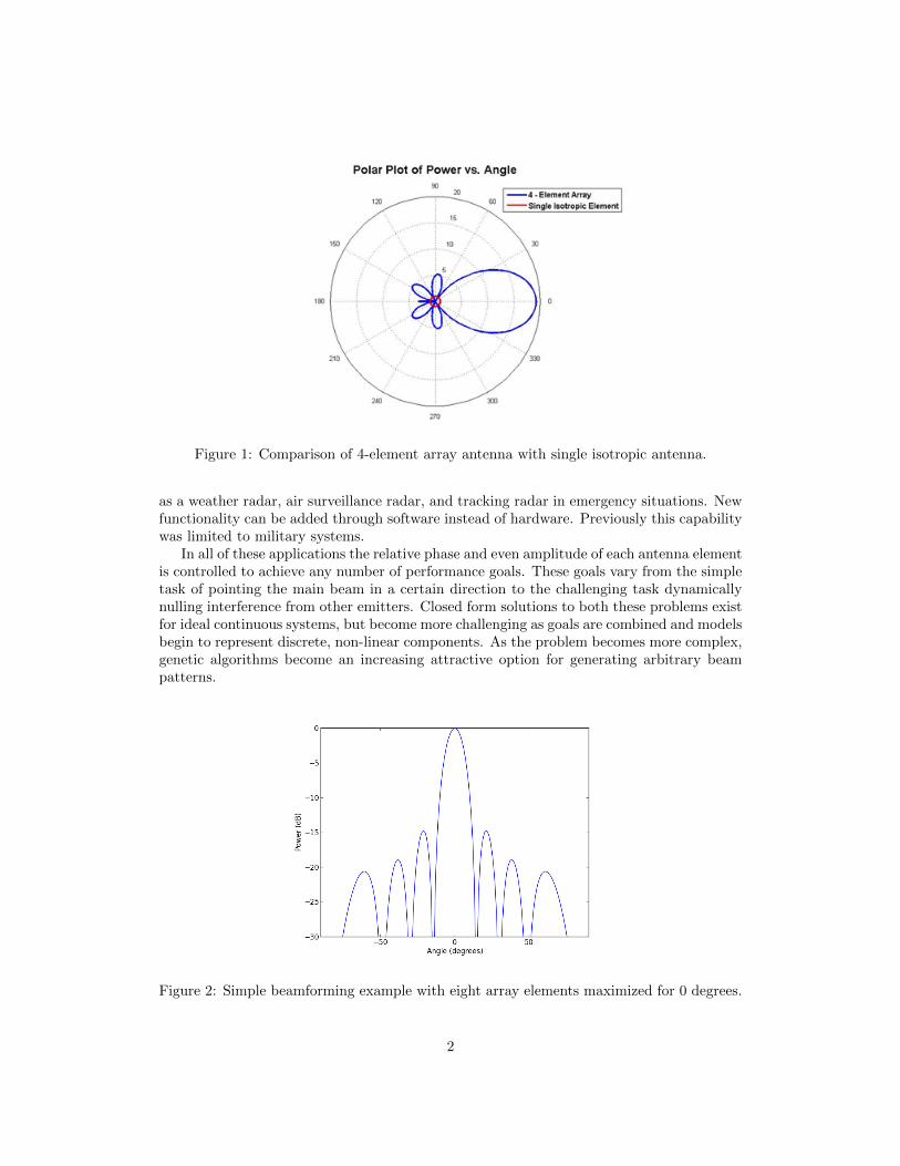
Figure 1: Comparison of 4-element array antenna with single isotropic antenna.

as a weather radar, air surveillance radar, and tracking radar in emergency situations. Newfunctionality can be added through software instead of hardware. Previously this capabilitywas limited to military systems.

In all of these applications the relative phase and even amplitude of each antenna elementis controlled to achieve any number of performance goals. These goals vary from the simpletask of pointing the main beam in a certain direction to the challenging task dynamicallynulling interference from other emitters. Closed form solutions to both these problems existfor ideal continuous systems, but become more challenging as goals are combined and modelsbegin to represent discrete, non-linear components. As the problem becomes more complex,genetic algorithms become an increasing attractive option for generating arbitrary beampatterns.

Figure 2: Simple beamforming example with eight array elements maximized for 0 degrees.

2

2 Project Objective

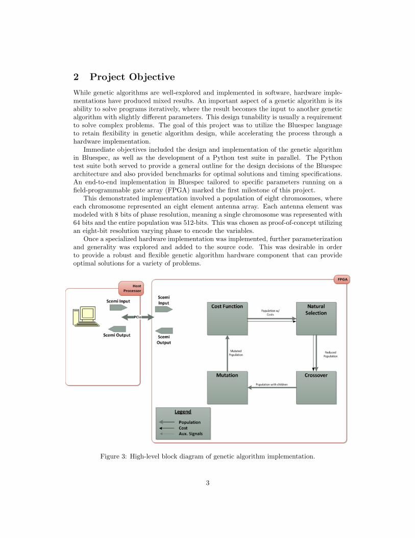
While genetic algorithms are well-explored and implemented in software, hardware imple-mentations have produced mixed results. An important aspect of a genetic algorithm is itsability to solve programs iteratively, where the result becomes the input to another geneticalgorithm with slightly different parameters. This design tunability is usually a requirementto solve complex problems. The goal of this project was to utilize the Bluespec languageto retain flexibility in genetic algorithm design, while accelerating the process through ahardware implementation.

Immediate objectives included the design and implementation of the genetic algorithmin Bluespec, as well as the development of a Python test suite in parallel. The Pythontest suite both served to provide a general outline for the design decisions of the Bluespecarchitecture and also provided benchmarks for optimal solutions and timing specifications.An end-to-end implementation in Bluespec tailored to specific parameters running on afield-programmable gate array (FPGA) marked the first milestone of this project.

This demonstrated implementation involved a population of eight chromosomes, whereeach chromosome represented an eight element antenna array. Each antenna element wasmodeled with 8 bits of phase resolution, meaning a single chromosome was represented with64 bits and the entire population was 512-bits. This was chosen as proof-of-concept utilizingan eight-bit resolution varying phase to encode the variables.

Once a specialized hardware implementation was implemented, further parameterizationand generality was explored and added to the source code. This was desirable in orderto provide a robust and flexible genetic algorithm hardware component that can provideoptimal solutions for a variety of problems.

Figure 3: High-level block diagram of genetic algorithm implementation.

3

3 High-Level Design

The general anatomy of the genetic algorithm was based very loosely on the evolutionarymodel found in nature. A population is composed of sets of dependent variables (chromo-somes) in which some chromosomes have a higher fitness (higher cost function) than others.The strongest chromosomes from a population “mate” to produce “offspring,” while theweakest chromosomes die off in order to maintain a constant population size.

From the surviving chromosomes, the “fittest” are chosen to mate to produce offspring,which fill the gap left by the removal of weak chromosomes. Random chromosome muta-tion is typically introduced as a method to avoid local minima. After several generations,the population grows to resemble the optimal solution; arbitrary mutation enables uniquesolutions to arise.

Genetic algorithms offer a lot of flexibility to the designer in choosing how specificallyeach step is executed. For example, there are a wide range of documented methods forcombining genes from parents to create offspring. This flexibility can be leveraged to tunethe general framework to a specific problem, and allow for unconventional but semi-optimalsolutions to previously solved problems.

4 Test Plan

4.1 Python Testing Suite

Hardware and software codesign was especially important to this project, not only to re-alize the final implementation, but also to test and validate modules along the way. Toreliably test the implementation of genetic algorithms, a standard benchmark was requiredfor validating that the resulting population is indeed an optimal collection of chromosomes.The majority of the process that is outlined previously was tested by developing softwarebenchmarks that emulated the evolutionary process.

The genetic algorithm.py testing file is a Python simulation of the implementation offlexible genetic algorithms. The previous iteration of the code was limited to two variablearithmetic operations, and could be configured to either deliver the maximum or minimumsolution. The possible values that could be input were two four-bit binary numbers, thereforeresulting in a total of eight bit chromosomes that are passed between the functions.

The second and most recent iteration of the code steered the algorithm to resolve aspecific problem: complex antenna beamforming. Given a population of randomly generatedchromosomes (represented as an eight element of eight-bit variables), an angle, numberof deaths per generation, and number of iterations, the program will return an optimalchromosome to maximize power and efficiency for beamforming.

The code structure calls four primary functions that represent the first three steps inthe proposed pseudo code: cost function, natural selection, crossover, and mutation. Theprimary data structure that is passed around is an array of integers ranging from -128 to 127(possible expression with eight-bits) that represent the various specimen of each generation.All four functions take a population as input and return an altered population array basedon the required function. The main function call provides the arguments required for all fourfunctions and executes them in order, updating the population at each step, and iteratingthe entire process for a specified number of generations.

The first step is to create a random population using generate population, which createsan array of random chromosomes. Then, the cost function, which evaluates the input func-

4

tion based on the various members of the population using a helper method calculate cost.Each chromosome represents an array of eight eight-bit binary values ranging from -128to 127. The cost is calculated as described previously. Once the costs are computed, thepopulation array is sorted based on the cost function result.

Next, the second step takes place in natural selection, which simply drops off the worsttwo members of the population. Because the input population array is already sorted bycost function, natural selection can assume that the last two chromosomes of the array arethe worst performing.

The third step is cross over, which calls a tournament selection method that returnstwo of the strongest parents from two randomly-selected pools. The random mask functionrandomly distributes the indices of the chromosome length among two arrays. These twoarrays are used to determine which child gets which index of a parent, and the arraysare swapped for each child, therefore creating two children. The resulting population willtherefore be the same length as the input population, since two new children of the twostrongest parents are appended to the array.

Finally, the last step of the genetic algorithm is mutate, which randomly selects froma pool of every chromosome except for the strongest one, in order to ensure that the bestperforming is untouched. Then, a random value within the array of the chromosome ischanged to a random number. This completes a generation of the genetic algorithm andcan be repeated to optimize the population.

The strength in this testing suite is the ability to test each module by comparing it to thecorresponding function. Therefore, it was simple to test each step of the genetic algorithmas it ran alongside the proposed test suite. The randomness associated with the mutationstep requires it to be removed in the majority of testing so that a deterministic system canbe evaluated and compared. The block were then tested in isolation and added back intothe system if needed.

A simple problem, such as a 2D surface optimization, was used to validate the modulesand architecture as they were developed. This allowed rapid testing without the overheadof in-depth optimization for the complex antenna problem.

4.2 Bluespec Simulation Testbench

Bluespec’s simulation environment was used heavily to test both the individual modules andentire Bluespec design. Building a unique testbench for each module provided confidencethat each module was functioning as expected before it was added to the overall design.Typically these testbenches involved two rules representing inputs and outputs; however,for some of the modules an initiation rule was needed as well. Another testbench modulewas built to wrap the entire genetic algorithm module.

This testbench provided a way to evaluate the module interface methods, the data flowwithin the module, and the transient startup and shutdown procedures. The testbench wasalso useful because it provided a major debug step before the SceMi interface was added tocommunicate with software. Finally, Bluespec simulation was used to test and debug thehardware/software interface before the design was moved to the FPGA.

5 Microarchitectural Description

This implementation of genetic algorithms for solving complex beamforming problems uti-lizes four primary modules: antenna cost, natural selection, crossover, and mutation, in that

5

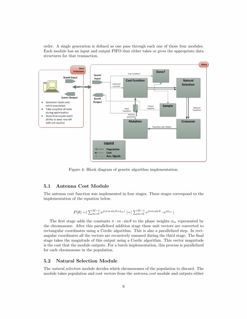
order. A single generation is defined as one pass through each one of those four modules.Each module has an input and output FIFO that either takes or gives the appropriate datastructures for that transaction.

Figure 4: Block diagram of genetic algorithm implementation.

5.1 Antenna Cost Module

The antenna cost function was implemented in four stages. These stages correspond to theimplementation of the equation below.

P (θ) =|∑M−1m=0 e

j(πm sin θ+φm) |=|∑M−1m=0 e

jπm sin θ · ejφm |

The first stage adds the constants π ·m · sin θ to the phase weights φm represented bythe chromosome. After this parallelized addition stage these unit vectors are converted torectangular coordinates using a Cordic algorithm. This is also a parallelized step. In rect-angular coordinates all the vectors are recursively summed during the third stage. The finalstage takes the magnitude of this output using a Cordic algorithm. This vector magnitudeis the cost that the module outputs. For a batch implementation, this process is parallelizedfor each chromosome in the population.

5.2 Natural Selection Module

The natural selection module decides which chromosomes of the population to discard. Themodule takes population and cost vectors from the antenna cost module and outputs either

6

a population vector or both population and cost vectors to crossover. Below are descriptionsof different implementations with unique advantages and disadvantages.

5.2.1 Find Max/Min

One implementation of natural selection that was tried was a “find M min of N” algorithm.The motivation was to reduce the number of sorting steps compared to a full sorting al-gorithm. The disadvantage was that the produces an unsorted population of reduced sizefor the crossover module. As a result the crossover module needs to be passed the costfunction. A similar algorithm was implemented in the “top two” implementation of thecrossover module.

5.2.2 Bubblesort

This implementation of natural selection utilizes a simple Bubblesort algorithm as an alter-native to explicitly passing on an associated cost vector. As an input, the module takes apopulation vector and cost vector. The corresponding cost of a given chromosome is at thesame index, so the cost of the first chromosome is the first element of the cost vector.

Figure 5: Using Bubblesort to sort a simple sequence of numbers.

Once the input tuple containing both population and cost vectors is unpacked, the sortingalgorithm begins. Bubblesort iterates through the cost array, comparing if the current costis less than the next cost. If so, it swaps the index of the corresponding chromosomes inthe population vector. In worst case scenarios, this would be on the order of log(n2), sinceBubblesort is a quadratic sorting algorithm.

Once the population vector is sorted with the maximum cost first and in decreasingorder, this module outputs only that vector. This simplifies the interfaces for the followingmodules since the cost vector is no longer required; it is implicitly encoded as the indices ofthe population vector.

5.2.3 Thresholding

The use of a specific threshold is the most direct and efficient method for large populationsdue to the scaled cost of sorting. A running average is maintained and compared to eachsample and depending on if the sample is above or below the threshold then the sample iseither kept or discarded.

5.3 Crossover Module

The crossover module is tasked with selecting the parents to mate in order to producechildren that replace the previously removed members of the population. Various schemescan be used to select the parent chromosomes to mate, two explored by this implementationare described below. The disadvantage is that the number of chromosome removed fromthe population each generation is variable.

7

Figure 6: Simple alternating mask applied to two parents to produce children.

5.3.1 Top Two Selection

The simplest way to select parents for each generation would be to use the top two per-forming members according to the cost function. While this approach is fast and does notrequire much computation beyond identifying the maximum (either explicitly or through asorted array), it does limit the evolution of a population to a certain amount of spontaneity.Forcing the top two parents to produce children could potentially limit the algorithm toa optimal solution that actually represents a local maximum,, not the global maximum.Therefore, while this approach is attractive for rapid development, it can be altered orreplaced in order to increase population variety.

5.3.2 Tournament Selection

Another potential method of selecting parents could be a tournament style process. Chromo-somes are split randomly into a number of pools, and each “winner” of the pool is determinedand advanced to another round to face the another pool “winner”. These rounds continueuntil only two winners are left standing. This allows for some flexibility in selecting parents;it is assured that the parents will not always be only the two fittest chromosomes.

Figure 7: Simple tournament selection for parents.

5.3.3 Mating

Once the parents are selected, the children chromosome can be produced by applying a bitmask. The mask is a simple binary template (of length chromosome size) that determineswhich parent to copy the bit from, and switches for each child. It is important to distinguishthe difference between bit-level switching and variable-level switching; this implementationviews each chromosome as a 64-bit string and changes one bit among that 64, while anotherpotential method would be to change an entire variable (a sequential block of 8 bits in the

8

example case). This degree of masking can be controlled and another factor that can affectthe rate and diversity of evolution within the genetic algorithm.

At its most fundamental representation, any level of masked mating is accomplished atthe bit-level, which ultimately resulted in this particular implementation. Once the childrenare produced, they are inserted back into the vector and crossover returns the population.

5.4 Mutation Module

Once the children are added into the population data structure, the mutation module “mu-tates” a randomly selected member from a pool of chromosomes composed of every one fromthe population except for the best performing. This is enforced in order to make sure thatthe strongest chromosome is left untouched and continues to survive as is until the nextgeneration.

A random chromosome is selected from the population (using Bluespec functionality inthe LFSR package). Once the target is selected, a single bit of its composition is flipped.The index of this bit is randomly selected, so the degree of change can be minor to major.Therefore, such a change would result in a new chromosome in the population. Once thisis done, the population is returned, ready for another iteration of the genetic algorithm.

Figure 8: Example of mutating a single bit of a mutant.

5.5 Genetic Algorithm Processor

The genetic algorithm processor module ties together the four modules described below inaddition to implementing the functionality seen by the user. The module was implementedwith four states, described below.

• WAIT - This is the initial state that the design comes up in by default. In this state,the design accepts all user input including an initial population, the initial constantsfor the antenna cost function, and the stop conditions. The methods that load in thevalues are guarded so that they only fire in the WAIT state.

• INIT - The INIT state is used for the transient startup behavior of the design. Oncethe user inputs a start command, the design enters this state. In this state the designloads all initial inputs into the appropriate module. Once this is complete the designenters the RUN state.

• RUN - This state contains the normal behavior of the processor. Data is passed frommodule-to-module within the processor. A sample input can be received from the user,which takes a snapshot of the state the processor is in and sends it back to the user.This state continues until a stop command is received externally or a stop conditionis met within the module.

9

• DONE - In this state data flow has stopped within the processor. Sample commandscan still be received to take a snapshot of the final state the processor was in. Tech-nically this command can be reached from any other state without any issues (usinga stop command), but the transition is intended to be from RUN to DONE.

Once the processor has reached the DONE condition, a reset signal is need to transitionback to the WAIT state to start a new optimization. This is because unpredictable behaviorcan arise from a initializing the design with data still in the pipeline.

5.6 SceMi Layer Module

The SceMi Layer Module acts as the Bluespec interpreter to the outside world. More im-portantly, the module is outfitted with the proper action value methods that can extract therelevant output information and package it into bits that the outside world can understand.This layer of abstraction simply called on the genetic algorithm Bluespec code and packagedthe bits for output, as well as understood the C++ inputs to initialize and test the geneticalgorithm. The start signal to the genetic algorithm was also administer at this stage.

Figure 9: Simulation results of costs versus generation.

5.7 Test Bench

Actual testing of this implementation was done in the C++ and Python programminglanguages. C++ served as a interface between the host computer and the FPGA/Bluespecsimulation. The C++ would utilize SceMi to interpret the bits coming out of the Bluespecside and output the desired information to a text file. Once the data was stored in a textfile, a Python script was utilized to plot the information.

Python was used for its robust mathematical functionality and simple plotting libraries;the entire testing procedure was initialized by a testing script which delivers end to endresults by taking user input, running the test, and actively opening a plot directory anddisplaying plots of the strongest chromosome growing over time.

10

Figure 10: Command line interface for running test bench.

6 Implementation Evaluation and Performance

The modules described in the previous sections were initially implemented in sequentialpipeline. The entire population passes from module to module and the functionality ofeach module is implemented on the entire population at once. This architecture allowedtraditional genetic algorithm approaches from software to be most easily implemented. Dueto deficiencies in the hardware implementation of a sequential approach, fully pipelinedapproach was later implemented with significant performance increases.

Figure 11: Initial implementation performance.

6.1 Sequential Implementation

The initial sequential implementation was modeled off of a traditional software implementa-tion of a genetic algorithm. Each stage executes in series and the entire population datasetmoves between modules in a single step. This allowed tradition genetic algorithm softwaretechniques to be implemented with little modification. These traditional techniques typ-ically involve operations on the entire population such as sorting, averaging, or random

11

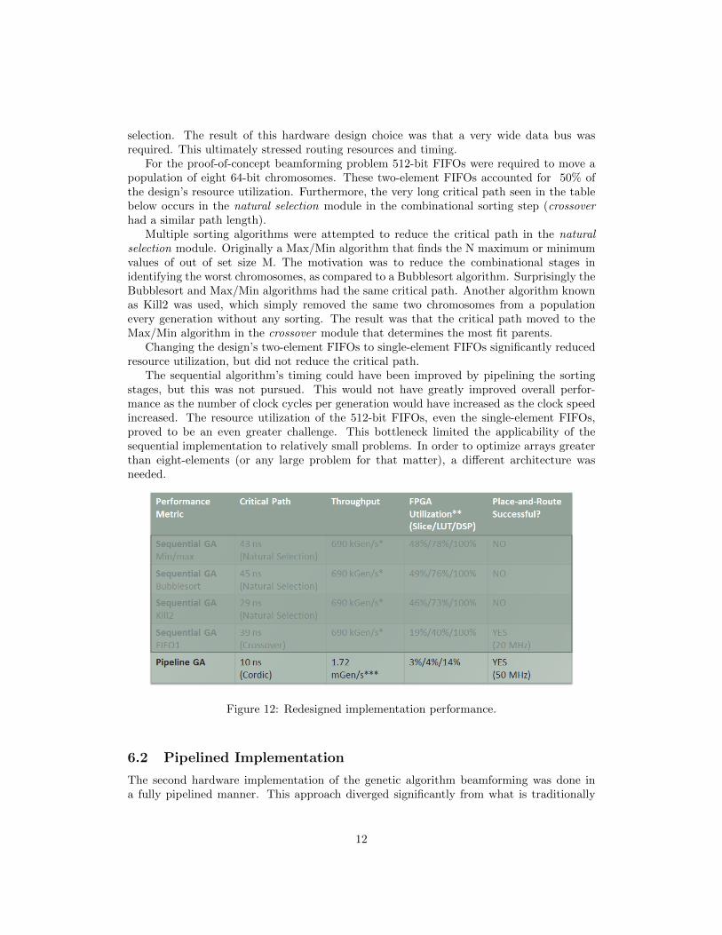
selection. The result of this hardware design choice was that a very wide data bus wasrequired. This ultimately stressed routing resources and timing.

For the proof-of-concept beamforming problem 512-bit FIFOs were required to move apopulation of eight 64-bit chromosomes. These two-element FIFOs accounted for 50% ofthe design’s resource utilization. Furthermore, the very long critical path seen in the tablebelow occurs in the natural selection module in the combinational sorting step (crossoverhad a similar path length).

Multiple sorting algorithms were attempted to reduce the critical path in the naturalselection module. Originally a Max/Min algorithm that finds the N maximum or minimumvalues of out of set size M. The motivation was to reduce the combinational stages inidentifying the worst chromosomes, as compared to a Bubblesort algorithm. Surprisingly theBubblesort and Max/Min algorithms had the same critical path. Another algorithm knownas Kill2 was used, which simply removed the same two chromosomes from a populationevery generation without any sorting. The result was that the critical path moved to theMax/Min algorithm in the crossover module that determines the most fit parents.

Changing the design’s two-element FIFOs to single-element FIFOs significantly reducedresource utilization, but did not reduce the critical path.

The sequential algorithm’s timing could have been improved by pipelining the sortingstages, but this was not pursued. This would not have greatly improved overall perfor-mance as the number of clock cycles per generation would have increased as the clock speedincreased. The resource utilization of the 512-bit FIFOs, even the single-element FIFOs,proved to be an even greater challenge. This bottleneck limited the applicability of thesequential implementation to relatively small problems. In order to optimize arrays greaterthan eight-elements (or any large problem for that matter), a different architecture wasneeded.

Figure 12: Redesigned implementation performance.

6.2 Pipelined Implementation

The second hardware implementation of the genetic algorithm beamforming was done ina fully pipelined manner. This approach diverged significantly from what is traditionally

12

done in software, but is not the first time the approach has been tried.2 Instead of movingtogether, the population is stretched out over the length of the processing chain. As a result,algorithms need to be chosen for each module that do not require the entire population toaccumulate at each step. In fact, in the demonstrated implementation each module bothaccepts and produces a chromosome every clock cycle. This resulted in the highest possiblethroughput for any given clock speed.

6.2.1 Cost Function Module

In order to achieve this throughput in the antenna cost function, a pipelined Cordic processorwas needed. The Cordic processor leveraged from earlier coursework was folded so that itwould only accept an input at the end of each cycle.

Unfolding the design in a parameterized way required Bluespec’s Maybe type and newguards so that the pipeline would fill and drain properly. The resources used by the addi-tional stages were more than made up for by the fact that only one chromosome is evaluatedat a time, instead of all in parallel. The critical path in this model was 10 ns.

Figure 13: Cost function block diagram.

13

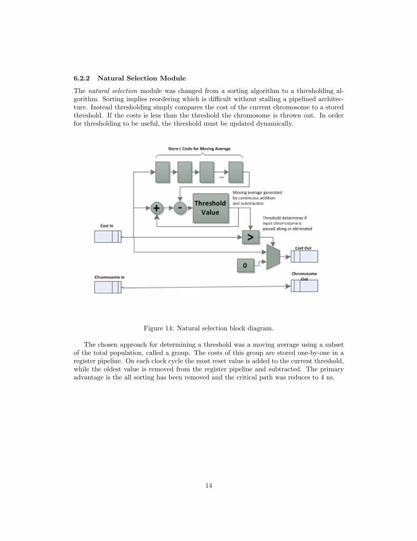
6.2.2 Natural Selection Module

The natural selection module was changed from a sorting algorithm to a thresholding al-gorithm. Sorting implies reordering which is difficult without stalling a pipelined architec-ture. Instead thresholding simply compares the cost of the current chromosome to a storedthreshold. If the costs is less than the threshold the chromosome is thrown out. In orderfor thresholding to be useful, the threshold must be updated dynamically.

Figure 14: Natural selection block diagram.

The chosen approach for determining a threshold was a moving average using a subsetof the total population, called a group. The costs of this group are stored one-by-one in aregister pipeline. On each clock cycle the most reset value is added to the current threshold,while the oldest value is removed from the register pipeline and subtracted. The primaryadvantage is the all sorting has been removed and the critical path was reduces to 4 ns.

14

6.2.3 Crossover Module

Crossover was migrated to a tournament selection, also using a group sub-set of chromo-somes. In this module the group represents the current mating pool. On each clock cyclethe module can one of two functions. If it does not receive a valid chromosome from naturalselection (meaning that it has been removed) if performs parent selections and crossover.Otherwise it updates the mating pool with the most recent valid chromosome and passesthe chromosome along unchanged.

Figure 15: Crossover block diagram.

If parent selection and crossover occurs, linear feedback shift registers (LFSRs) are usedto generate four random indices that point to values in the mating pool. Pairs of potentialchromosomes are compared to produce two parents. These parents are then mated using amask generated by a separate LFSR to produce a new chromosome.

15

6.2.4 Mutation Module

Mutation needed to be modified as well to support a pipeline architecture. More specificallyinstead of choosing which chromosome to mutate, the module now needed to determine ifthe chromosome would be mutated or not. These odds could be generated with an LFSRand a fixed threshold to set the odds a mutation will occur on a given chromosome.

Figure 16: Mutation block diagram.

The module also needed to keep track of the best chromosome it has seen and not mutateany chromosome with a higher cost. This protected the entire algorithm from regressing.Finally a second LFSR was used to determine which bit in the chromosome was mutated ifa mutation did occur.

7 Design Exploration

With the pipeline architecture implemented and proven, a number of design exploration canbe undertaken. The first of which is determining the scaling limits on the architecture interms of chromosome size. This explorations has begun, but could continue further. Theexample design described and demonstrated above used a 64-bit chromosome representing an8-element antenna array with 8 bits of phase resolution. For the Virtex 5 device used a designusing a chromosome size of 256-bits (32 elements) was successfully compiled and routed fora 50 MHz device clock. Resource utilization was modest (27%Slice/28%LUT/50%DSP).The convergence rate of the larger model has not been tested yet. Furthermore, synthesisof the algorithm on other devices was explored as well. A synthesis on a Virtex 7 (VC707Eval Board) was also explored. A 1024-bit (128 element) architecture was synthesized wasa 8 ns critical path and very low resource utilization (13%Slice/25%LUT/4%DSP). While it

16

was not attempted it is believe this design could be successfully implemented on the devicewith a 100 MHz clock. This brief exploration implies that this pipelined architecture couldbe scaled to model even some of the largest antenna arrays with current FPGA technology.The next step would be to explore how long it takes the optimization to converge given theimmense number of degrees of freedom. If these problems converge in less than roughly abillion generations (5 minutes at 100 MHz) this tool could find many applications.

Other design explorations would include more complex antenna cost functions such asminimizing angular ripple, controlling side lobe levels, or modeling multiple frequency bandsat once. Ultimately these would be implemented with an increased degree of parallelizationof the Cordic models.

A final design exploration would be to investigate the applicability of the pipelined GAarchitecture to other problem sets. On limiting factor might be the architectures benefitsare largely related to the fact that the antenna cost can be pipelined. This might not beimplemented so easily with other problems. Otherwise the overall structure is very modularand parameterized, with modules utilizing a common interface. It is anticipated that thisproject could form the code base for future genetic algorithm hardware implementations.

17

References

[1] Haupt, Randy L. Genetic Algorithms in Electromagnetics. 1st Ed. Wiley-IEEE Press,2007. Print.

[2] Sheu, Shiann-Tsong, and Yue-Ru Chuang. “A Pipeline-Based Genetic Algorithm Ac-celerator for Time-Critical Processes in Real-Time Systems.” IEEE Transactions onComputers. 55.11 (Nov. 2006): 1435-1448. Print.

18