Hardware Implementation Of An Object Contour DetectorUsing Morphological Operators

Master thesis performed in Electronics Systemsby

Hisham Berjass

LiTH-ISY-EX--10/4283--SELinköping, 10/12/08

Hardware Implementation Of An Object Contour DetectorUsing Morphological Operators

Master thesis in Electronics Systemsat the Department of Electrical Engineering

Linköping Institute of Technologyby

Hisham Berjass

LiTH-ISY-EX--10/4283--SELinköping 10/12/08

Supervisor: Kent PalmqvistExaminer : Kent Palmqvist

Language

English

Number of Pages

42

Type of Publication

X Licentiate thesis Degree thesis Thesis C-level Thesis D-level Report Other (specify below)

ISBN (Licentiate thesis)

ISRN:LiTH-ISY-EX---10/4283---SE

Title of series (Licentiate thesis)

Series number/ISSN (Licentiate thesis)URL, Electronic Version

http:

Abstract

The purpose of this study was the hardware implementation of a real time moving object contour extraction.

Segmentation of image frames to isolate moving objects followed by contour extraction using digital

morphology was carried out in this work. Segmentation using temporal difference with median thresholding

approach was implemented, experimental methods were used to determine the suitable morphological operators

along with their structuring elements dimensions to provide the optimum contour extraction.

The detector with image resolution of 1280 x1024 pixels and frame rate of 60 Hz was successfully implemented,

the results indicate the effect of proper use of morphological operators for post processing and contour

extraction on the overall efficiency of the system. An alternative segmentation method based on Stauffer &

Grimson algorithm was investigated and proposed which promises better system performance at the expense of

image resolution and frame rate.

Keywords

Object detection, FPGA, Morphological operators, Contour extraction, Segmentation, Image processing.

Department and Division

Department of Electrical EngineeringDepartment of Electronics System

Publication TitleHardware Implementation Of An Object Contour Detector Using Morphological Operators AuthorHisham Berjass

Presentation Date

2010/12/07

Publishing Date (Electronic version)

Acknowledgments

First and foremost, I offer my sincerest gratitude to my supervisor, Kent Palmqvist, who has

supported me throughout my thesis with his patience and knowledge whilst allowing me the room to

work in my own way.

Finally but not least, I would like to show my gratitude to my parents who supported me in every

possible way.

Abstract

The purpose of this study was the hardware implementation of a real time moving object contour

extraction. Segmentation of image frames to isolate moving objects followed by contour extraction

using digital morphology was carried out in this work. Segmentation using temporal difference with

median thresholding approach was implemented, experimental methods were used to determine the

suitable morphological operators along with their structuring elements dimensions to provide the

optimum contour extraction.

The detector with image resolution of 1280 x1024 pixels and frame rate of 60 Hz was successfully

implemented, the results indicate the effect of proper use of morphological operators for post

processing and contour extraction on the overall efficiency of the system. An alternative

segmentation method based on Stauffer & Grimson algorithm was investigated and proposed which

promises better system performance at the expense of image resolution and frame rate.

Table of Contents

Chapter 1 .....................................................................................................................1 Introduction ............................................................................................................................1

1.1 Overview............................................................................................................................1 1.2 Objectives ..........................................................................................................................1 1.3 Thesis organization ............................................................................................................2

Chapter 2 .....................................................................................................................3 Theoretical Background...............................................................................................................3

2.1 Object Detection ................................................................................................................3 2.2 Digital Morphology ...........................................................................................................6

2.2.1 Erosion .......................................................................................................................8 2.2.2 Dilation ......................................................................................................................8 2.2.3 Opening .....................................................................................................................9 2.2.4 Closing .....................................................................................................................10

2.3 System conceptual design ................................................................................................11Chapter 3 ...................................................................................................................13 Implementation approach ..........................................................................................................13

3.1 MATLAB implementation................................................................................................13 3.2 HDL implementation........................................................................................................14

Chapter 4 ..................................................................................................................21 Simulation and Testing ..............................................................................................................21

4.1 Functional Verification ....................................................................................................21 4.2 Results..............................................................................................................................25

Chapter 5 ...................................................................................................................27 Design environment and System Integration.............................................................................27

5.1 System Description ..........................................................................................................27 5.2 Synthesis and device utilization.......................................................................................30

Chapter 6 ...................................................................................................................32 Proposed system upgrade...........................................................................................................32

6.1 Algorithm modifications ..................................................................................................32Chapter 7 ...................................................................................................................37 Conclusion and Future work .....................................................................................................37

7.1 Future work .....................................................................................................................37 7.2 Conclusion .......................................................................................................................38

Reference.....................................................................................................................39Appendix ....................................................................................................................41

Chapter 1 Introduction

This thesis work presents a hardware implementation of a object contour detector which involves

the computational exhaustive task of segmentation and simple yet powerful tools of morphology

for post processing and contour extraction. The motivation of the thesis work involving why a

dedicated hardware is used instead of a general purpose hardware, is presented in this chapter and

how various morphological operators can be tuned and cascaded for contour extraction is presented

through out this work.

1.1 Overview

Object detection and feature extraction are active research areas in video processing and computer

vision, many of today's applications extending over different fields including medical industrial and

surveillance utilize these techniques, most of these applications require special demands regarding

power, size, weight and real time computational capability.

Moving object detection is mainly performed by segmentation where the moving object or the object

of interest is isolated from the background. Multitude of software algorithms that perform

segmentation and feature extraction have been proposed and implemented but their computational

complexity and their lack of real time compatibility makes their use unfeasible in most applications.

Software implementation of object detection and feature extraction running on general purpose

computers are restricted to small image resolution and frame rates.

This work presents a hardware implementation of a moving object contour detector, focusing on the

post segmentation processing and contour extraction using digital morphology.

1.2 Objectives

The main objectives of this work are

• To create a contour object detector module with effective segmentation and contour

extraction capability, with frame rate of 30 Hz and acceptable image resolution.

1

• To investigate the optimum SE and mask dimensions of the various morphological operator

blocks to obtain the best contour extraction results.

• To integrate the contour object detection module with the camera example provided by

Altera which targets DE-2 educational board platform.

The system was successfully implemented on DE2-70 educational board from Altera with a

TRDB_D5M camera mounted on the board's expansion port, the design assumes that the camera is

fixed and targets an indoor environment where the intensity variation is limited. The system

performs segmentation based on temporal difference with median thresholding method to

distinguish the moving object then performs successive morphological operations for post

processing and feature extraction.

1.3 Thesis organization

The second chapter of the work starts by familiarizing the reader with the basic needed theoretical

background, from there the implementation approach in software and hardware of the object

detection module is described in chapter 3. Chapter 4 covers the simulation and verification of the

object detection module and states the results obtained.

Since the system utilizes an existing design provided by Altera, Chapter 5 describes the integration

of the object detector module described in chapter 3 with the existing design.

Chapter 6 describes an alternative approach for system implementation, the thesis ends with chapter

7 by a conclusion about the conducted work and methods for future system upgrade.

2

Chapter 2 Theoretical Background

This chapter presents the theoretical basis on which this thesis was built, the system implemented

can be divided into two basic parts object detection, and image processing using digital morphology.

The former has been widely covered in many literature with many available techniques and

approaches while the later is definite in its concept and implementation.

The choice of the object detection techniques covered in this study depends on their feasibility of

being practically implemented on the targeted hardware. The chapter concludes with the choice of

the conceptual design that describes the system.

2.1 Object Detection

Real time segmentation of moving objects classifies the image pixels into either foreground (moving

objects) or background. A common approach of such a classification is background removal, known

as background subtraction. Segmentation is performed by comparing each video frame against a

reference background model. Pixels that deviate slightly from the background are considered to be

moving objects, this is performed by comparing each pixel in the resultant difference frame against a

threshold value.

According to Cheung and Kamath [1], most of the available background removal algorithms follow

the four major steps.

(1) Pre-processing used to change the raw image data to a format that can be used in later

stages.

(2) Background modeling.

(3) Foreground detection.

(4) Post-processing used to eliminate those pixels that do not correspond to actual moving

objects.

3

The background modeling is the major step in determining how efficient a certain background

subtraction algorithm performs. In the simplest case a non adaptive algorithm is used where a static

background with no moving objects is taken as a reference background. The incoming video

sequence is compared against it to detect any new object that is introduced to the background.

Manual initialization is required in such an algorithm otherwise errors in the background accumulate

over time making this method not efficient in most cases.

A standard method for adaptive background algorithm is averaging the images over time to obtain a

background approximation similar to the current static scene except where motion occurs. Although

this method might be efficient in cases where object moves continuously and the background is

visible for a significant amount of time, it poorly performs in situations where the object moves

slowly. In addition it can not handle multi-modal background distributions which are caused by

small repetitive movements in the background (e.g. swaying of trees) and changes in the scene

intensity which is the case in real environments [2].

Stauffer & Grimson algorithm [3] represents an adaptive method which uses a mixture of Gaussians

(MoG) to model the values of a particular pixel instead of single distribution to model the values of

all the pixels as in the previous methods.

Based on persistence and variance of each of the Gaussians representing a pixel, background pixels

are determined, pixel values that do not fit the distribution within a certain tolerance are labeled as

foreground. Since several Guassians are used, it correctly models multi-modal distributions and

since the parameters of the Guassians are continually updated, its able to adjust to changing

illumination and to gradually learn to model the background.

MoG algorithm

Pixel process is defined as a time series of pixel values e.g. vectors for color images. At any time t

the history of a particular pixel {xO ,yO} is

{X1

, ...., Xt}={I x

o, y

o, i :1≤i≤t}

where I is the image sequence.

4

Every pixel is modeled as a mixture K (three to five) Gaussian distributions. The probability of

observing the given value of a current pixel is

P Xt=∑i=1

K wi , t∗X

t,

i , t,

i , t

Where K is the number of distributions, w i,t is an estimated weight of the i th Gaussian in the

mixture at time t, µ i,t is its mean value, ∑ i,t is its covariance matrix and η is a Gaussian probability

density function

Xt

, ,= 12

n2∣∣

12e

12 X

t−

tT∑−1 X

t−

t

For computational reasons, the red, blue and green pixel values are assumed to be independent and

have the same variances then

k=diag

k

2

Every new pixel value Xt is checked against the existing K Gaussian distributions, until a match is

found, a match is defined as a 2.5 standard deviations (2.5σ) of a distribution. The weight, mean and

the variance parameters of the distribution are updated as

wk , t=1− w

k , t−1

t=1−

t−1X

t

2=1− 2

t−1X

t−

tT X

t−

t

where μ and σ2 are the mean and variance respectively, α and ρ are the learning factors,and Xt are

the incoming RGB values.

For those unmatched, the mean and variance remain the same while the weight is updated according

to

wk , t=1− w

k , t−1

5

If non of the K distributions match the current pixel value, the least probable distribution is replaced

with a distribution with the current value as its mean and a high variance.

Since the parameters are updated frame by frame the Guassians are then ordered by the decreasing

value of w/σ, this value increases when the distribution gains more evidence and when variance

decreases. This ordering of the model guaranties that the most likely background distributions

remain on top while the less probable transient background distributions gravitate towards the

bottom and are eventually replaced by new distributions.

The portion of the Gaussian distributions belonging to the background is determined by

B=argminb

∑k=1b w

kT

where T is a predefined parameter and wk is the weight of distribution k, if a small value of T is

chosen, the background model is usually uni-modal which results in less processing, while choosing

a higher value of T results in a multi-modal background model capable of handling periodic

repetitive motion in the background.

2.2 Digital Morphology

According to [6], the mathematical morphology is an image processing method used for extracting

image components that are useful in representation and description of region shape such as

boundaries or skeletons, also morphological techniques can be used for pre-post processing such as

morphological filtering, thinning, and pruning.

Mathematical morphology is built on the set theory, the sets in mathematical morphology represent

objects in an image, for example the set of all white pixels in a binary image is a complete

morphological description of an image.

In binary images, the sets are members of a 2-D integer space Z 2 where each element is a 2-D

vector whose coordinates are the (x,y) coordinates of a white pixel in the image. Mathematical

morphology can be further extended to gray images but its not in the scope of this work.

6

Based on [4], morphological operators are neighborhood operators i.e they performs an operation

on a region of pixels at a time, this is realized using a structuring element (SE). SE can be viewed as

a shape, used to probe or interact with a given image, with the purpose of drawing conclusions on

how this shape fits or misses the shapes in the image, examples of structuring elements are given in

Figure 2.1.

The set A of shaded elements constitute the structural element, a computer implementation requires

that the set A be converted to a rectangular array (a mask) by adding background elements, when

dealing with binary image through out the discussion the structuring elements (shaded regions) have

a value of logical “1” while the background elements correspond to logical “0”, the same goes for

the image being scanned by the structuring element where the object pixel is represented by logical

“1” and that of a background as a logical “0”.

When scanning a binary image with a mask, for example the first mask from the left of Figure 2.1

Which is a 5x5 cross mask, the center of the mask is positioned over the pixel being processed. An

operation is performed utilizing all the image pixels under the SE, this is repeated until all the image

pixels are scanned.

It should be noted that there is some special cases where there are some parts of the mask that are

outside the image border. In such cases background pixels must be added to the image such that the

mask is always a subset of the image being scan, this is known as zero padding.

The morphological operators utilized in this work are that of erosion and dilation. These operators

are the fundamental morphological operators, opening and closing are also considered which are

composites of the fundamental operators.

7

Figure 2.1: Structuring elements with origin at the middle pixel

2.2.1 Erosion

With A and B are sets in E=Z 2 , an integer grid, the erosion of A by B, denoted as

,

where A is the image set being scanned, B being the structuring element and Bz is the translation of

B by a vector z, the equation indicates that the erosion of A by B is the set of all points z such that B,

translated by z, is contained in A.

In Figure 2.2, a binary image with an object (dark blue) is eroded by the 3x3 cross mask then the

object in the resultant image will be shrink-ed. The green region of the eroded image represents the

part of the object that has been removed and now is a part of the background, thus erosion can be

viewed as a morphological filtering operation in which image details smaller than the structuring

element are filtered (removed) from the image [4,5].

2.2.2 Dilation

With A and B are sets in E=Z 2 , an integer grid, the Dilation of A by B, denoted as

,

where A is the image set being scanned, B being the structuring element and Bs is the symmetric of

B, the equation is based on reflecting B about its origin and shifting this reflection by z.The dilation

of A by B then is the set of all displacements, z, such that Bs and A overlap by at least one element.

8

Figure 2.2:Binary image A to the left ,Eroded image in the middle ,cross shaped structuring element to the right

Background pixelObject pixelRemoved object pixel

Background pixelObject pixelRemoved object pixel

Unlike erosion, which is a shrinking or thinning operation, dilation “grows” or “thickens” objects in

a binary image as it shows in Figure 2.3. The specific manner and extent of this thickening is

controlled by the shape of the structuring element used. The green region represents the part of the

background that has been added and is now a part of the object as a result of dilation [4,5].

2.2.3 Opening

From the elementary erosion and dilation operations, opening and closing operations are developed.

If an image with multiple objects is considered, the erosion operator is useful for removing small

objects, however it has the disadvantage that all the remaining objects shrink in size Figure 2.4. This

effect can be avoided by dilating the image after erosion with the same structuring element. This

combination of operation is called opening operation. The opening of set A by structuring element B

is defined as

9

Figure 2.3:Binary image A to the left ,Eroded image in the middle ,cross shaped structuring element to the right

Background pixelObject pixelAdded object pixel

Background pixelObject pixelAdded object pixel

Figure 2.4:Binary image A to the left ,Opened image in the middle ,cross shaped structuring element to the right

Background pixelObject pixelBackground pixelObject pixel

As its clear in the Figure 2.5, opening removes out objects which at no point, completely contain the

structure element, but avoids general shrinking of object size, it can also be noted that the object

boundaries become smoother [4,5].

2.2.4 Closing

As has been discussed, the dilation operator enlarges objects and closes small holes and cracks,

general enlargement of objects by the size of the structuring element can be reversed by a following

erosion. This combination of operations is called closing operation.

The closing of set A by structuring element B is defined as

10

Figure 2.6:Binary image A to the left ,Opened image in the middle ,cross shaped structuring element to the right

Background pixelObject pixelBackground pixelObject pixel

Figure 2.5:Binary image A to the left ,Opened image to the right using cross shaped structuring element

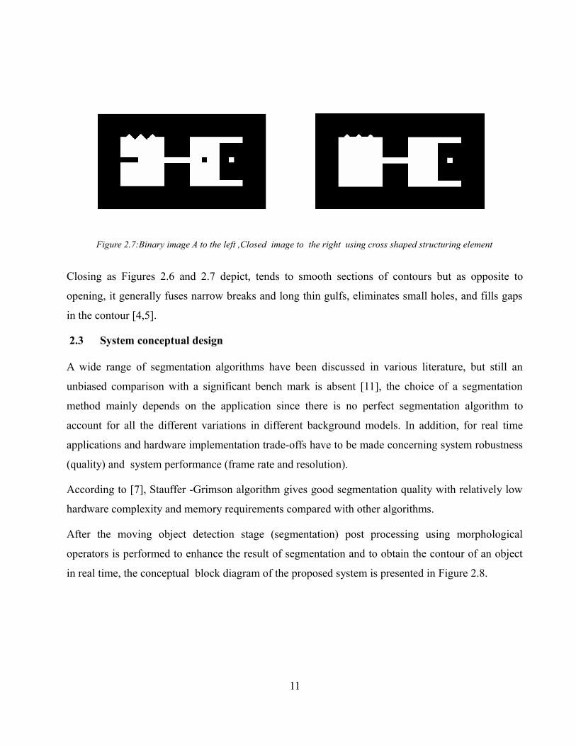
Closing as Figures 2.6 and 2.7 depict, tends to smooth sections of contours but as opposite to

opening, it generally fuses narrow breaks and long thin gulfs, eliminates small holes, and fills gaps

in the contour [4,5].

2.3 System conceptual design

A wide range of segmentation algorithms have been discussed in various literature, but still an

unbiased comparison with a significant bench mark is absent [11], the choice of a segmentation

method mainly depends on the application since there is no perfect segmentation algorithm to

account for all the different variations in different background models. In addition, for real time

applications and hardware implementation trade-offs have to be made concerning system robustness

(quality) and system performance (frame rate and resolution).

According to [7], Stauffer -Grimson algorithm gives good segmentation quality with relatively low

hardware complexity and memory requirements compared with other algorithms.

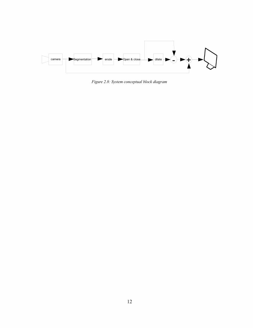
After the moving object detection stage (segmentation) post processing using morphological

operators is performed to enhance the result of segmentation and to obtain the contour of an object

in real time, the conceptual block diagram of the proposed system is presented in Figure 2.8.

11

Figure 2.7:Binary image A to the left ,Closed image to the right using cross shaped structuring element

12

Figure 2.8: System conceptual block diagram

-camera Segmentation erode Open & close dilate +

Chapter 3 Implementation approach

This chapter discusses the implementation of the object contour detector based on background

subtraction method both in software using MATLAB and hardware using HDL, the chapter

continues with the description of the design environment and platform used for system

implementation.

3.1 MATLAB implementation

Image processing usually involves matrix-based computations which is strongly supported in

MATLAB, in addition to the availability of an image processing toolbox with built-in functions.

The algorithm was first implemented in MATLAB to check its functionality since the mask selection

and the structuring elements sizes used in Morphological operators were based on trial and error.

Thus, using a software tool for prototyping have paid by reducing the design time.

Object detector implementation in MATLAB

In a MATLAB file an image frame representing the Background is read into a one dimensional gray-

scale matrix. A new frame representing the object in the scene is read into another matrix. The

matrices are converted to type double suitable for arithmetic operations. Segmentation is performed

by obtaining the absolute difference of the two frames then thresholding using a median threshold

that is the average intensity value. The obtained matrix is transformed to type logical so that binary

morphological operations can later be performed.

Morphological built in functions are then performed using predefined structuring elements, erosion

followed by Open and Close and then Dilation.

Finally, the Dilated and Closed image frames are subtracted to obtain the object contour which is

later overlaid over the original input frame.

Extension of the above algorithm to operate on RGB images is straight forward, since the same

operation will be performed on the three components.

The MATLAB implementation of the algorithm is provided in the Appendix.

13

3.2 HDL implementation

The targeted platform being an FPGA, the hardware implementation was realized on a DE2-70

educational board from Altera. Both hardware descriptive languages VHDL and Verilog were used

since the object detector exploits the DE2 camera example which uses Verilog. VHDL was used in

the object contour detector module since the author is more familiar with that language.

Object contour detector

This module reads video stream and background image from the 4_Port SD_RAM controllers. The

read operation is started by the sync_cntrl module which enables reading from the 2 output ports of

the SD_RAM controller. The function of the module is to continuously compare the streamed in

video with a pre-defined background. It uses image difference, thresholding and morphological

operators in order to pinpoint out the detected object by extracting its contour and overlaying it on

the original streamed in video frame. The output processed image frame is then sent to the VGA

controller to be displayed.

The module is made of several sub-modules as shown in Figure 3.1.

14

Figure 3.1:Object contour detector architecture

f_sync

Dynamic_buffer_1

pxl_clk

sy nc_cntrl fsyncrsync

iRequest

OD_rst rst RST

Difference Overlay

P_pixel

iRequest

Dynamic_buffer_2

DilateOpen/CloseSegmentation ErodeImagedifference

B_pixel

v_pixel

Control signals

The sync_cntrl sub-module generates the row and frame synchronization signals (rsync and fsync)

to all the sub-modules of the object contour detector as well as the input request (iRequest) for

acquiring the video and background pixel data from the SD RAM (V_pixel and B_pixel), the

synchronization signals should match those of the VGA controller in order to correctly display the

processed image on the VGA.

The OD_rst sub-module provides the reset signals to all the other sub-modules.

Segmentation

This is performed by image_difference sub-module which subtracts the incoming frame from a fixed

background in order to isolate the new introduced object. The operation is done on the three

components R,G and B, its hardware implementation is simply an exclusive-or operation performed

on a each pixel per clock (pxl_clk).

In order to distinguish the object from the background thresholding is used. Each of the pixel

components is compared to its corresponding threshold value to determine if it belongs to the

background or to the object. If the pixel component is greater than the corresponding threshold then

its a foreground pixel and thus given a value of logical '1' else its a background pixel and given a

value of logical '0'.

The median method is used to obtain the thresholds of the three pixel components. Thus the

implemented segmentation is based on temporal difference with median thresholding.

Morphological operations

The binary morphological operations used (erode/dilate) utilize the same approach to process an

image. The image (logical format ) is scanned by a mask, and in order to perform a certain function

on a certain pixel, the mask must be positioned with its center over that pixel. The output is a

function of the center pixel and its neighbors that are under the structuring element. Two mask sizes

have been implemented 3x3 and 5x5 masks.

The architecture to perform a certain morphological operation is shown in Figure 3.2.

15

The mask_buff sub-module forms the mask that scans the image frame, it utilizes inputs from other

sub-modules. Line buffer sub-module whose dimensions depend on the mask size, stores rows of

image data. Mask state sub-module which provides the position of the mask relative to the image

frame being scanned and pixel switch sub-module which responsible for border padding.

The mask data is then sent to the Erode/Dilate sub-module where a structuring element is selected to

perform erosion or dilation.

line_buffer

The line buffer is used to store 2 rows of a frame (when a 3x3 mask is used) and 4 rows of a frame

(when a 5 x 5 mask is used). This module is created using Altera's mega wizard function. The line

buffer has a length of the image width in this case 1280 pixels with two taps as shown in Figure 3.3.

16

Figure 3.2 Dilate/Erode module architecture

pdata_in

rsy nc

f sy nc

rst

pclk_in

mask_buf fnxn

mask _statepdata_out

Erode/Dilate

Pixel Switch1

line_buf f

Pixel Switch nxn

n denotes the size of the mask

mask_buff

This module creates the state machine for scanning the mask over the image, the input data is

obtained from the line buffer and the latest input pixel.

mask_state

Is a 10 state machine to control the position of the mask over the image, the output is two bit vectors

Vx and Vy that determine which row or column of the mask is outside the image border, this is used

in Pixel switch sub-module to insert zeros in such places Figure 3.4.

S0 :The initial state of the mask, the process must wait in this state until it has a valid data under the

mask for example in case of a 3x3 mask and an input image of 1280x1024 resolution, the process

must wait (1280 +1) pixel clock cycles before it moves to the next state .

S1:The first active state where the mask is centered over the first pixel (upper left corner of an

image frame), at this point the first processed pixel is present at the output that is after (1281+3)

pixel clock cycles.

S2 :The upper non corner state, the process stays in this state as the mask scans from left to right the

first row until it reaches pixel 1279 (in case of 3x3 mask ) then it switches to the next state.

S3:The upper right corner state, where the mask is centered over the last pixel of the first raw.

S4:The non corner left edge state, after S3 the mask returns back to the beginning of the second row

with its center over the first pixel in that row.

S5:The center state, where there is no parts of the mask outside the frame border.

17

Figure 3.3 :Line buffer for 3x3 mask

tapsx1

shift in tapsx0

1281 2561

1280 1

S6:The non corner right edge state, where the third column of the mask is outside the frame border.

S7:The lower left corner state, where column one and third row are outside the image frame border.

S8:The lower non corner state, where only the third row is outside the image frame.

S9:The lower right corner state, where both the third row and column of the mask are outside the

image frame.

Pixel switch

This module takes a data pixel under the mask from the mask_buff module, its position in the mask,

and Vx and Vy (define the mask position relative to the image) from the mask_state module to

check whether the data pixel is valid (i-e lies within the image frame) or non valid (i-e lies outside

the image frame). The valid pixel is passed to the erode/dilate module else if the data pixel is not

valid then it is switched to zero (zero padding) before passing it to the erode/dilate module.

In the case of using a 3x3 mask then 9 instances of this module are created, one for each pixel in the

mask.

18

Figure 3.4 :3x3 mask scan over an image frame with zero padding

Erosion/Dilation

Once the data under the mask is passed to this module, operation is straight forward. The structuring

element selected for implementing erosion or dilation based on MATLAB simulation for optimum

results is shown below.

The highlighted parts represent the structuring element and it

includes pixels (P2,P4,P5,P6,and P8). The output located at

the center of the mask will be :

An AND operation on the pixels under the structuring

element in case of Erosion.

An OR operation on the pixels under the structuring element

in case of Dilation.

Dynamic buffers

The dynamic buffers that are used to compensate for either the delay of the dilate module in the

upper video path or for (image_difference, segmentation, erode, open/close, dilate and difference)

modules in the lower video path. These are FIFO buffers created using Altera's mega wizard

function. Table 3.1 shows the delays of different components in the object contour detector module

which are used to calculate the size of the dynamic buffers.

Table 3.1: Input /output delay of the different sub-modules.

Component Delay between input and output

Image_difference 1 pixel clock cycle

Thresholding 1 pixel clock cycle

Erode 2x1280+4 pixel clock cycles (5x5 structuring element)

Open/close 4(1280+4) pixel clock cycles (3x3 structuring element )

Dilate 2x1280+4 pixel clock cycles (5x5 structuring element)

Difference 1 pixel clock cycle

Overlay 1 pixel clock cycle

Dynamic buffer_2 1 +1+2(2x1280+4)+4(1280+4) +1=10275 pixel clock cycles

Dynamic buffer_1 2x1280+4 = 2564 pixel clock cycles

19

Figure 3.5 : mask structuring element

P7 P8 P9

P1 P2 P3

P4 P5 P6

Dynamic_buffer_1

The size of the Dynamic_buffer_1 can be determined by the time the dilate module takes in order to

produce the first valid pixel Table 3.1. Since the mask size in that module is 5x5 then the first valid

pixel will be after (2x1280+4) pixel clock cycles, so the dimension of this FIFO will be 2564 bit

length and 1 bit depth.

Dynamic_buffer_2

This FIFO buffer should compensate for (image_difference,segmentation,erode,open /close, dilate

and difference modules), so that the object contour produced by the upper path could be overlaid

correctly on the relative image frame.

From Table 3.1, the first valid pixel that will appear at the input of the overlay module from the

upper path will be after 10275 pixel clock cycles, then the dimensions of the FIFO buffer will be of

length 10275 and depth of 30.

Object contour extraction and Overlay

The Eroded image frame is subtracted from the Dilated one in the Difference module to obtain the

object contour. Synchronization between the two frames is ensured by the Dynamic_buffer_1

module. Difference is performed by a pixel-wise exclusive-or operation in VHDL.

The detected object contour is then overlaid over the original image frame which contains the object

in the scene. Dynamic_buffer_2 module ensures the synchronization between these two frames.

This is done by changing the value of the R,G and B components in the buffered image frame to

maximum component intensity in case the corresponding pixel in the processed image frame has a

value of logical '1'.

20

Chapter 4 Simulation and Testing

This chapter presents the procedure taken to ensure that the system functionality meets the

specifications, MODELSIM and MATLAB were used to perform the functional verification of the

Contour object detector module.

4.1 Functional Verification

The verification method used is mainly simulation-based verification of functionality, test benches

are constructed that simulate the design under verification.

Since the system is composed of modules which are in turn formed of sub-modules, the correctness

of the sub-modules and modules is a prerequisite for verifying the entire system. Thus a bottom-up

verification strategy is performed, once the functional verification of bottom components is ensured

then these components can be integrated into the next level subsystem which is then verified. The

process is repeated up to the top level of the system .

Functional verification of the sub-module parts is straight forward since at that level the

functionality is rather simple; predefined stimuli Figure 4.1 is directly applied to the sub-modules

and the response is analyzed and compared with the expected response and accordingly the design is

modified until the verification is passed.

21

Figure 4.1: model sim testbench model

Test StimuliModule

under test

response

Stimuli

Test bench

At the module level where each module is expected to perform a definite image processing

functionality as stated by the specification, image frame is applied as a stimuli and the response

frame is compared with the output of the behavioral model created in MATLAB.

To successfully process images in this project, an interface between MATLAB and VHDL was

designed. Thus images captured were first processed with MATLAB into file formats acceptable for

processing in VHDL. Conversely, to view images processed in VHDL another design was used to

convert the data into MATLAB format.

After the functional verification of each module separately, functional coverage is performed where

functional verification is performed on successive modules joined in steps, this process is repeated

until all the modules are joined. Thus the functionality of the contour object detector is covered and

verified.

The most crucial part in the process of verification was to ensure the synchronization between the

different modules, i.e when should each module receive an input frame and start to process it and

how should the processed pixel frame reach the VGA controller. This is important since the contour

object detector is the module that reads from the memory and not the VGA controller, thus proper

frame and row synchronization signals were properly assigned through simulation.

22

Figure 4.2: Background ground image, image with introduced person, (640 x480) image resolution with 8 bit pixel depth

23

Figure 4.3: Image difference using MATLAB on the left, VHDL on the right.

Figure 4.4: Image thresholding using MATLAB on the left, VHDL on the right.

Figure 4.5: Image erosion,5X5 SE, using MATLAB on the left, VHDL on the right.

24

Figure 4.8: Image difference using MATLAB on the left, VHDL on the right.

Figure 4.7: Image dilation,5x5 SE, using MATLAB on the left, VHDL on the right.

Figure 4.6: Image opening and closing, 3x3 SE, using MATLAB on the left, VHDL on the right.

4.2 Results

The above figures show that the functionality of the algorithm implemented in VHDL is similar to

that in MATLAB. Its clear from the first difference operation Figure 4.3 there is a higher precision in

MATLAB than in VHDL, since the later utilizes bit vectors of constant length to represent pixels

while in MATLAB pixels were represented by integers of type double.

But the result is somehow balanced in the thresholding stage since the threshold in MATLAB will

be lower than that in VHDL due to the noise introduced by the difference operation. As a result more

noise will be extracted by the lower threshold as its shown in Figure 4.4.

A close inspection on the result of the first difference Figure 4.3 where the object is being extracted

indicates that some parts of the object disappeared. This is an inherent problem of background

subtraction technique since pixels of the object that have close intensity value to that of the

corresponding background pixels will not be detected as foreground. Selecting a low threshold will

improve the result but at the expense of increased noise. Most if not all segmentation techniques

used nowadays for object detection result in noise and miss detection of parts of an object but with

varying performances. Although the implemented segmentation above which is background

difference with thresholding, that is considered to be the least efficient method, but as shown from

the results above applying morphological operations after the segmentation step reduces the noise

and helps in filling missing object parts and smoothing its boundaries.

25

Figure 4.9: Image overlay using MATLAB on the left, VHDL on the right.

The effectiveness of a certain morphological operation applied on an image depends mostly on the

size and shape of the mask. The largest mask dimension applied here is 5x5 mask for dilation and

erosion and a 3x3 mask for opening and closing, thus the algorithm fails in removing noise regions

that are larger than 5x5 pixels and filling missing parts that are larger than 3x3 pixels.

Although the first erosion results in a significant noise reduction but its effect is also widening the

missing parts in the object. A better effective approach is by replacing the erosion by another open

and close stage, the improvement is clearly visible in Figure 4.9 with further reduction of noise since

the first opening is performed with a 9x9 mask, its implementation in hardware guarantees better

performance but at the expense of higher hardware cost and higher delay in the video path.

26

Figure 4.10: Contour detection using open close operation instead of erosion as a first stage

Chapter 5 Design environment and System Integration

This chapter describes the modification performed on the camera example provided by Altera to fit

the system requirements. The chapter also presents the functional description and hardware

utilization of each module in the system.

5.1 System Description

The design platform is formed of DE2-70 educational board from Altera with a 5 mega pixel

(TRDB-D5M) camera which can be mounted on the board's expansion port, a keyboard and a VGA

screen, the design also utilizes the camera example Verilog modules provided by Altera [8].

Apart from the Contour object detector all the modules are taken from the DE_2 camera example

with changes to fit the system requirements. As Figure 5.1 shows the Video path formed of CCD

Capture, RAW2RGB and SDRAM controller is duplicated, one for continues video stream and the

other for background capture. The difference of the two paths is that the Capture module of the

background path is able to start or stop feeding image frames to the SD RAM controller, this

27

Figure 5.1:System conceptual block diagram

CCD Sensor

(TRDB-D5M)

SD-RAM0 VGA-DAC

I2C CCD conf igure

CCD Capture RAW2RGB

4 Port SD-RAMController1

VGA _Controller

Key board

SD-RAM1

CCD Capture RAW2RGB 4 Port SD-RAM

Controller1

KB-interf aceCore

DE2_70 Board

VGA

Contour Object Detector

Video stream

Background image

start end

guaranties that the contour object detector reads the same frame from the SD RAM in case the end

button is pressed or goes back to continuous streaming in case the start button is pressed in order to

allow the selection of a new background image.

CCD Sensor

Pixels are output in a Bayer pattern format consisting of four colors Green1, Green2, Red, and Blue

(G1,G2, R, B) representing three filter colors, each four adjacent pixels will be used to produce a

corresponding RGB pixel by the RAW2RGB module. The pixel array structure is formed of three

regions, an active image in the center surrounded by an active boundary and then a dark boundary.

When the image is read out of the sensor, it is read one row at a time, with the rows and columns

sequenced as shown in Figure 5.2.

The image read out is controlled by FRAME_VALID and LINE_VALID signals that are

synchronized to pixel clock, at every pixel clock when both FRAME_VALID and LINE_VALID

signals are asserted a pixel is read out [9].

CCD control registers

The CCD sensor has registers that can be configured which makes the output data format flexible.

By default the sensor produces 1,944 rows of 2,592 columns with no binning or skipping, reads only

the active image without the boundaries, the FRAME_VALID and LINE_VALID signal are asserted

at negative pixel clock.

28

Figure 5.2:Pixel colour pattern detail [9]

First clear Pixel

Column readout direction

Row

read

out d

irect

ion

Black Pixels

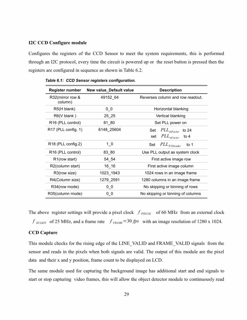
I2C CCD Configure module

Configures the registers of the CCD Sensor to meet the system requirements, this is performed

through an I2C protocol, every time the circuit is powered up or the reset button is pressed then the

registers are configured in sequence as shown in Table 6.2.

Table 6.1: CCD Sensor registers configuration.

Register number New value_Default value Description

R32(mirror row & column)

49152_64 Reverses column and row readout.

R5(H blank) 0_0 Horizontal blanking

R6(V blank ) 25_25 Vertical blanking

R16 (PLL control) 81_80 Set PLL power on

R17 (PLL config. 1) 6148_25604 Set PLLmFactor to 24 set PLLnFactor to 4

R18 (PLL config.2) 1_0 Set PLLP1Divider to 1

R16 (PLL control) 83_80 Use PLL output as system clock

R1(row start) 54_54 First active image row

R2(column start) 16_16 First active image column

R3(row size) 1023_1943 1024 rows in an image frame

R4(Column size) 1279_2591 1280 columns in an image frame

R34(row mode) 0_0 No skipping or binning of rows

R35(column mode) 0_0 No skipping or binning of columns

The above register settings will provide a pixel clock f PIXCLK of 60 MHz from an external clock

f XCLKIN of 25 MHz, and a frame rate f FRAME=30 fps with an image resolution of 1280 x 1024.

CCD Capture

This module checks for the rising edge of the LINE_VALID and FRAME_VALID signals from the

sensor and reads in the pixels when both signals are valid. The output of this module are the pixel

data and their x and y position, frame count to be displayed on LCD.

The same module used for capturing the background image has additional start and end signals to

start or stop capturing video frames, this will allow the object detector module to continuously read

29

the same frame stored in the SDRAM in case stop signal is asserted and update a frame if start and

stop push buttons are pressed in sequence.

RAW2 RGB

This module is made of a line buffer length 1280 and width of 2, it stores 2 rows of data pixel in

order to access the 4 pixel components (R ,G1,B,G2) and transform them to three pixel components

(R,G,B), the R and B components are mapped the same while G component is addition of G1 and

G2, the module utilizes the pixel data position x and y from the capture module for mapping.

The outputs of the module are the 3 pixel components (R,G,B) of 10 bit depth and the valid data

signal which will enable the write to the FIFO of the SDRAM controller.

4 Port SDRAM controller

The controller is formed of 4 FIFO buffers 2 for writing and 2 for reading with 16 bit wide and 512

word depth each. The FIFO's will allow both the Object contour detector and the RAW2RGB to

access the memory simultaneously at different read and write rates, the writing rate is 60 MHz as

defined by the f PIXCLK and the reading rate is 108 MHz as defined by the VGA, each input/output

port is able to write/read 1280 x 1024 pixels of depth 15 into the SDRAM, the first input port writes

15 bit data composed of 10 bits of the red component and 5 bits of the green component while the

second port writes 10 bits of the blue component and the remaining 5 bits of the green component,

reading from the ports is performed in the same manner. The SDRAM frequency is 166.7 MHz to

guarantee proper reading and writing from the corresponding FIFO buffers.

VGA controller

The VGA controller generates the synchronization, blanking signals and RGB pixel components

with an image resolution of 1280 x 1024(60Hz). The VGA controller operates at a frequency of 108

MHz generated by a dedicated PLL .

5.2 Synthesis and device utilization

The system was synthesized using Quartus II software from Altera, The targeted DE2-70 board is

equipped with two off-chip 256 Mbit synchronous DRAMs, and Cyclone II EP2C70F672C7 FPGA

30

with 68416 LE's, 1152000 memory bits and 4 PLLs. The design utilizes the two off chip RAMs and

2 PLLs for generating the clocks for the SD-RAM controllers, and the VGA controller.

The design utilization in terms of logical elements and memory bits for the different modules is

given in Table 6.2 and Table 6.3.

Table 6.2 : Hardware utilization for different blocks in the system

Logic Block Nr. of Logic Cells Memory bits

Contour Object Detector

1590 188384

SD_RAM_ctrl 1037 43008

RAW2RGB 297 46092

CCD_capture 100 0

VGA_ctrl 93 0

Table 6.2 : Hardware utilization of Contour Object Detector different sub-modules

Logic Block Nr. of Logic Cells Memory bits

s ync_cntrl 124 0

OD_rst 59 0

segmentation 153 0

erode5x5 201 5112

open_close3x3 727 10224

dilate5x5 198 5112

difference 2 0

overlay 31 0

dynamic_buffer1 43 4096

dynamic_buffer2 52 163840

31

32

Chapter 6Proposed system upgrade

This chapter explores the implementation of an alternative method of segmentation that has been

discussed in the theoretical part of this work proposed by Stauffer & Grimson namely MoG

algorithm. The implementation approach is based on the work done by [11] which is a variation of

MoG algorithm targeted for hardware implementation.

5.3 Algorithm modifications

As proposed by [11], color transformation from RGB to YCbC r space will result in a background

that can be modeled using a single distribution considering an indoor environment, in such case no

upper bound is needed to sort the updated Gaussian variables as proposed by the original algorithm.

This is due to the fact that one pixel cluster will not spread out is several distributions by color space

transformation to YCbC r as illumination changes. Thus the equation that determines the background

distribution is changed to

B=argminb

wkT this will result in automatic single or multi modal background model

without the need to adjust the value of T.

33

Figure 6.1: Modified system conceptual block diagram

CCD Sensor

VGA _Controller

VGA

SD-RAM1

4 Port SD-RAMController1

4 Port SD-RAMController2

I2C CCD configure

CCD Capture RAW2RGB

Segmentation Morphological Operations

SD-RAM0 VGA-DAC

coreContour Object Detector

DE2-70 board

As shown in Figure 6.1 instead of two video stream paths presented in the previous design, only

one is used. The input intensity and chrominance components are provided to the segmentation unit

through a 4 port SD-RAM controller1 that is capable of handling different clock frequencies of

writing and reading from it's ports. The SD-RAM controller2 is used to store the updated parameters

of the Gaussian mixture in SD-RAM1. The result of the segmentation unit is a frame of binary

image which is passed to the morphological operations unit which has the same functionality as

before. The resultant processed image frame is displayed on the VGA through the VGA controller.

The YCbCr components can be obtained from the RGB components through the following linear

transformations

Y=16 +65.481 x R +128.533 x G +24.966 x B.

Cb=128 – 37.797 x R - 74.203 x G +112.0 x B.

Cr=128 + 112.0 x R - 93.786 x G -18.214 x B.

The overhead in terms of hardware is not significant and can be further reduced by multiplication

with rounded integers .

In the implementation shown in Figure 6.2, three Gaussian variables are used, i.e each pixel has

three Gaussian distributions, the corresponding parameters of the Gaussian distributions are stored

in SDRAM1 .

For each incoming pixel from the SD-RAM controller1 the corresponding parameters are read from

SD-RAM controller2, decoded and compared against one another for a match. The output of the

matching block is a reordered Gaussian distribution with the matched distribution multiplexed to a

specific port. The Gaussian distributions are updated by the parameter update unit, the

Foreground/Background is then performed by checking the weight of the updated matched Gaussian

distribution, the resulting output is a binary stream with logical one representing the foreground and

logical zero representing the background. The updated Gaussian parameters are then sorted

according to their weight for use in the next frame. In order to reduce the memory bandwidth

requirements an encoding scheme is used which is based on pixel locality in succeeding

neighboring pixels.

34

Word length Reduction

According to the experimental results of [11], the computational complexity and memory

requirements involved in applying the parameter updating method can be reduced using a coarse

updating where instead of adding a small positive or negative fractional number to the current mean,

a value of 1 or -1 is added, the same approach can be applied to the variance with a step value of

0.25 used instead. Using this scheme only integers are needed to represent the mean leading to a

35

Figure 6.2 : Segmentation unit architecture as proposed by [11]

Wordlength Reduction

Unmatched parameter update

Parameter UpdateDecoding

Sorting

+/-1

+/- 0.25

X

X

/

X +

/ /

//

Mux

//

> /

>H

//

/

/Match

1-α1 α1

/

46

46 /16

16

30

30

[Weight]

[Weight]

[Mean,Variance]

[Mean,Variance]

46

[Mean]24

6 [Variance]

24

24

46

/

/

16

6[Variance] '1'[Weight] '0'

24

No_match

3 Guass/46x3

Encoding(Pixel Locality )

/

1

2

1

3

3x50

46x3

/

3 Guass

16/[Mean]

From SD-RAM0 controller YCbCr

SD-RAM1

controller

[Weight]16

1-α1

reduction of the word length from 18-22 down to 8 bits and 6 bits to represent the variance, 2 of

which account for the fractional part, along with 16 bits to represent the weight, thus the word length

of single Gaussian distribution can be reduced up to 43% as compared to the normal updating

scheme. In addition, the hardware complexity is reduced since multiplication by the learning factor

ρ is no longer needed.

Pixel Locality

For further memory bandwidth reduction and to make the design feasible for hardware

implementation, a data compression scheme is used [7], [10], [11] which utilizes similarities of

Gaussian distributions in adjacent areas. In practice each Gaussian distribution can be considered as

a three dimensional cube in the YCbCr space, where the center of the cube is composed of YCbCr

mean values and the the border to the center distance is specified by 2.5 times the variance value .

The degree of similarity between two distributions can be viewed as the percentage of overlap

between the two cubes, this can be obtained by checking the deviation of two cube centers with

respect to the border length, the reason of such a criteria lies in the fact that a pixel that matches one

distribution will most likely match the other, if they have enough overlapping volume. A threshold K

can be used to determine the degree in which two cubes are adjacent to each other according to

1Cr−

2Cr≤2.5K

1

2

1Cb

− 2Cb

≤2.5K 1

2

1Y−

2Y≤2.5K

1

2

Thus by only saving non-overlapping distributions along with the number of equivalent succeeding

distributions, memory bandwidth is reduced. The value of K is proportional to the memory

bandwidth reduction, a higher value results in a lower memory bandwidth, however more noise is

introduced to the binary image due to the increased error in the match checking phase. Fortunately

the noise is non-accumulating and can be removed by the morphological processes in the next stage.

36

Chapter 6 Conclusion and Future work

The implementation of the object detection using non adaptive background subtraction has a

dramatic effect on extracting the object contour in the subsequent stages, this is due to many factors

mainly change of illumination, camera noise, non-static background and shadows due to moving

objects in the scene. In addition, using a global threshold to separate the object from the background

results in the removal of some parts of the object. All these factors result in noise clusters in the

processed image that is hard to remove and holes in the detected objects that are hard to close using

morphological operations which in turn leads to false contour detections .

6.1 Future work

The major bottle neck in the implementation of the architecture proposed in chapter 6 is memory

bandwidth. To implement the proposed segmentation module certain system parameters should be

modified.

As stated in chapter 6 the Match module reads the YCbCr components of an incoming pixel (24

bits) from SD-RAM controller1, and at the same pixel clock the corresponding Gaussian

distributions (150 bits) are read from SD-RAM controller2. Since the SD-RAM controller can write

or read 32 bits at each pixel clock then SD-RAM controller2 must operate 5 times faster than SD-

RAM controller1.

The implemented design reads pixel components at a rate of 108 MHz from SD-RAM controller1

as defined by the VGA controller. The SD-RAM operates at a maximum frequency of 166.7 MHz

thus to make it feasible for the SD-RAM controller2 to read /write 5 times faster, the operational

frequency of the SD-RAM controller1 must be reduced to 25 MHz. As a result the operational

frequency of the SD-RAM controller2 would be 125 MHz which ensures the correct operation of

writing and reading to and from the SD-RAM.

This can be made possible by reducing the image resolution to 640 x 480 pixels with 8 bit pixel

depth. Therefore, the cam will output at a frame rate of 30 Hz with pixel clock of 19MHz and the

VGA controller will output at a frame rate of 60 Hz with pixel clock of 25 MHz.

37

6.2 Conclusion

The replacement of the segmentation module based on image difference and median thresholding

by the proposed segmentation architecture will ensure a more robust and efficient contour object

detection. The adaptive nature of the proposed architecture makes it possible to keep the background

properly updated unlike in the previous design where manual initialization is required since errors

tend to accumulate over time. Global threshold is replaced by a pixel allocation to a certain

distribution based on its variation from its mean. Thus the false removal of large regions of the

object is avoided, which in turn makes it easier for the morphological operators to later fill any gap

within the object. In addition, the proposed architecture has the ability to handle multi-model

background distributions that are caused by small repetitive motions in the background. All these

capabilities makes the proposed architecture a good choice for implementation, thus improving the

overall system performance.

38

Reference

[1] Cheung, S.-C. and C. Kamath, "Robust techniques for background subtraction in urban traffic video," Video Communications and Image Processing, Volume 5308, pp 881-892, SPIE Electronic Imaging, San Jose, January 2004, UCRL-JC-153846-ABS, UCRL-CONF-200706.

[2] Shireen Y. Elhabian, Khaled M. El-Sayed, Sumaya H.Ahmed (2008), “ Moving Object Detection in Spatial Domain using Background Removal Techniques -State-of-Art”, Recent Patents on Computer Science, Vol.1, No.1, pp.32-54.

[3] C. Stauffer and W. Grimson, (1999), “Adaptive background mixture models for real-time tracking,” in Proc. IEEE Conference on Computer Vision and Pattern Recognition.

[4] Rafael C. Gonzales and Richard E. Woods, (2008), Digital Image Processing, 3rd ed., Prentice Hall, New Jersey.

[5] Bernd Jähne, (2005), Digital image processing, 6th revised and extended edition, Springer.

[6] Tinku Acharya Achorga and Ajo K.Ray, (2005), Image processing principles and Applications, Wiley.

[7] Jiang H., Ardö H. Öwall, V., (2005), ”Hardware Accelerator Design for Video Segmentation with Multi-modal Background Modelling”.

[8] Terasic, (2008) ,”5 Mega Pixel Digital Camera Development Kit”, version 1.0, Terasic

Technologies.

[9] Terasic, (2009),”Terasic TRDB-D5M Hardware specification”, version 2.0, Terasic Technologies.

[10] M.M.Abutaleb, A. Hamdy, and E.M. Saad , (2008),”FPGA-Based Real-Time Video-Object Segmentation with Optimization Schemes”, International journal of circuits systems and signal processing, Vol 2, pp.78-86.

[11] Hongtu Jiang, (2007), “Design Issues in VLSI Implementation of Image Processing Hardware Accelerators Methodology and Implementation”, Ph.D. thesis Lund University, Sweden.

39

40

Appendix

MATLAB file used

IM_W= 1280;

IM_H=1024;

A=imread('background','jpg');

B=imread('forground','jpg');

A_D=double(A);

B_D=double(B);

Im_dif=abs(A_D-B_D);

x=sum(Im_dif);

total=sum(x);

Y=total/(IM_W*IM_H);

k=Im_dif;

for n=1:IM_H;

for r=1:IM_W;

if k(n,r)>Y;

k(n,r)=1;

elseif k(n,r)<Y;

k(n,r)=0;

else k(n,r)=0;

end;

end;

end;

K=logical(k);

S_E=[0,0,1,0,0;0,0,1,0,0;1,1,1,1,1;0,0,1,0,0;0,0,1,0,0];

S_E1=[0,1,0;1,1,1;0,1,0];

E_Im=imerode(K,S_E);

Open_Im=imopen(E_Im,S_E1);

41

Close_Im=imclose(Open_Im,S_E1);

D_Im=imdilate(Close_Im,S_E);

Obj_Con=imsubtract(D_Im,Close_Im);

IM_Overlay=B;

for p=1:IM_H;

for q=1:IM_W;

if Obj_Con(p,q) ==1;

IM_Overlay(p,q)=255;

else IM_Overlay(p,q)=B(p,q);

end

end

end

42