Haplotype Sharing by Accounting for the Mode of Inheritance · beneﬁts in some cases, for example...

Aus dem Institut fur Medizinische Biometrie und Statistik

der Universitat zu Lubeck

Direktor: Prof. Dr. rer. nat. Andreas Ziegler

Haplotype Sharing by Accounting for theMode of Inheritance

Inauguraldissertation

zur

Erlangung der Doktorwurde

der Universitat zu Lubeck

- Aus der Medizinischen Fakultat -

vorgelegt von

Adel Ali Ewhida

aus Tripolis, Libyen

Lubeck 2008

1. Berichterstatter: Prof. Dr. rer. nat. Andreas Ziegler

2. Berichterstatter: Prof. Dr. med. Alexandar Katalinic

Tag der mundlichen Prufung: 28.05.2009

Zum Druck genehmigt. Lubeck, den 28.05.2009

gez. Prof. Dr. med. Werner Solbach

– Dekan der Medizinischen Fakultat –

To my wife and special girls

Table of Contents

List of Figures iv

List of Tables v

1 Introduction 1

1.1 Genetic background of diseases . . . . . . . . . . . . . . . . . . . . . . 1

1.2 Linkage analysis . . . . . . . . . . . . . . . . . . . . . . . . . . . . . . . 4

1.3 Association analysis . . . . . . . . . . . . . . . . . . . . . . . . . . . . 5

1.3.1 Haplotype-based association analysiss . . . . . . . . . . . . . . 10

1.3.2 Haplotype assignment with unrelated individuals . . . . . . . 12

1.4 The objective of this thesis . . . . . . . . . . . . . . . . . . . . . . . . . 17

2 Material and Methods 18

2.1 Haplotype sharing analysis using Mantel statistics . . . . . . . . . . . 19

2.1.1 Mantel’s statistic for space-time clustering . . . . . . . . . . . 19

2.1.2 Application of Mantel’s statistic to haplotype sharing . . . . . 20

2.1.3 Novel haplotype sharing Mantel test statistics . . . . . . . . . 27

2.2 Assessment of statistical significance . . . . . . . . . . . . . . . . . . . 28

2.2.1 Monte Carlo Permutation . . . . . . . . . . . . . . . . . . . . . 28

2.2.2 Test based on the assumption of asymptotic distribution of

haplotype sharing Mantel statistics . . . . . . . . . . . . . . . . 29

2.2.3 Definition of quantile-quantile plot . . . . . . . . . . . . . . . . 34

i

Table of Contents

2.3 Adaptation of haplotype sharing Mantel statistics to missing data . . 34

2.4 New measure of genetic similarity of haplotype sharing Mantel statis-

tics . . . . . . . . . . . . . . . . . . . . . . . . . . . . . . . . . . . . . . 36

2.5 Case-control simulated data . . . . . . . . . . . . . . . . . . . . . . . . 38

2.5.1 Haplotype estimation assessment . . . . . . . . . . . . . . . . 39

2.5.2 Missing data generation . . . . . . . . . . . . . . . . . . . . . . 40

2.5.3 Genotyping errors data generation . . . . . . . . . . . . . . . . 40

2.6 Quantitative trait data . . . . . . . . . . . . . . . . . . . . . . . . . . . 42

2.7 Genetic Analysis Workshop 15 data . . . . . . . . . . . . . . . . . . . 43

2.7.1 Simulated data . . . . . . . . . . . . . . . . . . . . . . . . . . . 43

2.7.2 Candidate region of chromosome 18q . . . . . . . . . . . . . . 44

2.8 Software . . . . . . . . . . . . . . . . . . . . . . . . . . . . . . . . . . . 45

3 Results 46

3.1 Case-Control study analysis . . . . . . . . . . . . . . . . . . . . . . . . 46

3.1.1 Linkage disequilibrium pattern within the gene . . . . . . . . 49

3.1.2 True haplotypes versus best estimates . . . . . . . . . . . . . . 52

3.1.3 Missing data analysis . . . . . . . . . . . . . . . . . . . . . . . 55

3.1.4 Genotyping errors data analysis . . . . . . . . . . . . . . . . . 59

3.2 Quantitative trait data analysis . . . . . . . . . . . . . . . . . . . . . . 63

3.3 Comparison of different assumption of asymptotic distribution . . . 66

3.3.1 Results of model-based haplotype sharing Mantel test statistics 67

3.3.2 Results of model-free haplotype sharing Mantel test statistics 70

3.4 Analysis of the new measure of genetic similarity of haplotype shar-

ing Mantel statistics . . . . . . . . . . . . . . . . . . . . . . . . . . . . . 71

3.5 Analysis of the chromosome 18q candidate region for rheumatoid

arthritis . . . . . . . . . . . . . . . . . . . . . . . . . . . . . . . . . . . . 74

4 Discussion 77

5 Summary 81

ii

Table of Contents

6 Zusammenfassung 83

References 85

A Appendix 99

A.1 Tables . . . . . . . . . . . . . . . . . . . . . . . . . . . . . . . . . . . . . 99

Acknowledgments 109

Curriculum vitae 111

Publikation and Abstracts 113

iii

List of Figures

1.1 Haplotype inference without family genotype information . . . . . . 13

2.1 The shared length between two haplotypes . . . . . . . . . . . . . . . 22

2.2 Genetic similarity between two individuals . . . . . . . . . . . . . . . 25

2.3 The shared length for a pair of individuals . . . . . . . . . . . . . . . 26

3.1 Empirical power of the HS Mantel statistic using binary trait data . . 48

3.2 Empirical power of the HS Mantel statistics using quantitative trait data 65

3.3 A normal quantile-quantile plots for random samples of model-based

HS Mantel statistics . . . . . . . . . . . . . . . . . . . . . . . . . . . . . 68

3.4 A chi-square quantile-quantile plots for random samples of model-

based HS Mantel statistics . . . . . . . . . . . . . . . . . . . . . . . . . 69

3.5 A beta quantile-quantile plots for random samples of model-free HS

Mantel statistics . . . . . . . . . . . . . . . . . . . . . . . . . . . . . . . 70

3.6 Results of chromosomes 6, 18 and 3 using the HS Mantel statistics . . 73

3.7 Results of the HS Mantel test statistic methods for 2,300 SNPs . . . . 75

iv

List of Tables

2.1 Genotype penetrances for different disease models . . . . . . . . . . . 39

3.1 Empirical type I error of the HS Mantel statistics using binary trait data 49

3.2 Pearson product-moment correlation coefficients over all replicates . 50

3.3 Empirical type I error of the HS Mantel statistics using simulating

datasets with weak LD pattern . . . . . . . . . . . . . . . . . . . . . . 52

3.4 Empirical powers of the HS Mantel statistics using simulating datasets

with weak or strong LD patterns . . . . . . . . . . . . . . . . . . . . . 53

3.5 Empirical type I error of HS Mantel statistics for best estimate haplo-

types . . . . . . . . . . . . . . . . . . . . . . . . . . . . . . . . . . . . . 54

3.6 Empirical power of HS Mantel statistics for true and best estimate

haplotypes . . . . . . . . . . . . . . . . . . . . . . . . . . . . . . . . . . 54

3.7 Empirical type I error of the HS Mantel statistics using five approaches

to deal with incomplete individual haplotypes . . . . . . . . . . . . . 57

3.8 Empirical power of the HS Mantel statistics using five approaches to

deal with pattern 1 of Missing data. . . . . . . . . . . . . . . . . . . . 58

3.9 Empirical power of the HS Mantel statistics using five approaches to

deal with patterns 2 and 3 of Missing data. . . . . . . . . . . . . . . . 59

3.10 Empirical type I error of HS Mantel statistics based on datasets with

three different rates of genotyping errors . . . . . . . . . . . . . . . . 62

3.11 Empirical Power of HS Mantel statistics based on datasets with three

different rates of genotyping errors . . . . . . . . . . . . . . . . . . . . 63

v

List of Tables

3.12 Empirical type I error of the HS Mantel statistics using quantitative

trait data . . . . . . . . . . . . . . . . . . . . . . . . . . . . . . . . . . . 66

3.13 Summary results across all 100 replicates for chromosomes 3, 6 and 18 74

3.14 Selected regions on chromosome 18q after the second step . . . . . . 76

A.1 rs-number, position (bp) as provided be the NARAC consortium . . 99

vi

1 Introduction

1.1 Genetic background of diseases

Diseases with a genetic component, like other phenotypic traits, are usually distin-

guished as being either Mendelian or complex. Mendelian traits are characterized

by well-defined phenotypes, one or two genetic disease loci with high penetrance, a

small phenocopy rate and usually small susceptibility allele frequencies. This clear

genotype-phenotype relation results in a clear pattern of inheritance. Mendelian

diseases are usually rare in the population. Complex traits show a less clear relation-

ship between genotype and phenotype due to two or more of the following charac-

teristics: ill-defined phenotypes, incomplete penetrance, high phenocopy rate, ge-

netic heterogeneity, oligogenic or polygenic inheritance, epistasis, mitochondrial in-

heritance, imprinting, and an often large contribution of environmental influences

(Lander and Schork, 1994; Belmont and Leal, 2005; Gulcher and Stefansson, 2006).

Unfortunately, almost all common, non-infectious diseases have a genetic compo-

nent and fall into the category of complex traits. Examples are heart disease, cancer,

arthritis, asthma, diabetes, hypertension, lipid metabolism disorders, some forms of

Alzheimer’s disease, and depression. Many of these disorders are debilitating and

some are among the leading causes of death in the Western world. There is a lot

of interest in understanding these diseases better and in particular determining the

1

1 Introduction

extent to which genetics play a role in predisposing individuals to disease.

An important step towards understanding a genetic disease is to identify the gene,

or genes, that play a role in the disease etiology, and a first step towards identifying

a gene is to find its chromosomal location. This is called gene mapping. Disease-

gene mapping for complex diseases is more challenging than mapping genes for

Mendelian disorders due to genetic heterogeneity in which mutations in differ-

ent genes can cause the same disease phenotype (Lander and Schork, 1994; Risch,

2000; Ottman, 2005; Sepulveda et al., 2007; Tang et al., 2008). Other factors such

as incomplete penetrances, phenocopies and late age at disease onset also limit the

progress of complex disease gene mapping (Gillanders et al., 2006). Hence, disease-

gene mapping efforts for complex diseases have not been as successful as those for

Mendelian disorders (Weiss and Terwilliger, 2000; Todd, 2001; Tabor et al., 2002). For

example, the number of genes and environmental factors involved in schizophrenia

is not clear. The genes encoding dysbindin (DTNBP1) and neuregulin 1 (NRG1) are

considered to have strong evidence of association with schizophrenia (Owen et al.,

2005). Other genes such as ”disrupted in schizophrenia 1” (DISC1), ”D-amino-acid

oxidase” (DAO), ”D-amino-acid oxidase activator” (DAOA) and ”regulator of G-

protein signaling 4” (RGS4) still do not have convincing results for schizophrenia

(Owen et al., 2005).

Although 99.9% of the human genomes are identical between people, there are still

millions of differences among the 3.2 billion base pairs (Kruglyak and Nickerson,

2001). These genetic variations can cause phenotypic variations among people and

are potentially associated with traits or diseases. Genetic markers, which are nu-

cleotide variants with known positions, are often used for human disease analyses.

Several types of markers exist, such as Restriction Fragment Length Polymorphisms

(RFLP’s), microsatellites, and single nucleotide polymorphisms (SNPs). Markers

can be used to construct a genetic map, which can be used as a reference for disease-

2

1 Introduction

gene mapping (Dib et al., 1996). Researchers can genotype markers for studying

their relationship with diseases according to a genetic map. Botstein et al. (1980)

proposed the concept using RFLP’s as the markers to construct a genetic map. Later,

genetic maps were constructed using denser microsatellites (Murray et al., 1994; Dib

et al., 1996). SNPs, which usually contain two alleles, have drawn significant atten-

tion as markers for genetic disease-mapping studies due to their high abundance

across the human genome (Kruglyak, 1997; Sachidanandam et al., 2001). It was es-

timated that there are around 7.1 million SNPs with a minimal allele frequency of

at least 0.05 in the human population (Kruglyak and Nickerson, 2001). With the

completion of PHASE I of the HapMap Project, the number of SNPs in the public

database (dbSNP) increased from 2.6 million to 9.2 million (International HapMap

Consortium, 2005).

As genotyping cost has become cheaper and the process has become faster, genotyp-

ing for markers can be performed on a genome-wide scale, which produces a large

amount of marker data for analysis (Gunderson et al., 2005; Syvanen, 2005; Rabbee

and Speed, 2006; Xiao et al., 2007). Hence, statistical methods are required after

numerous markers are genotyped from collected samples. Two commonly used sta-

tistical methods are linkage and association (linkage disequilibrium) analyses (Lan-

der and Schork, 1994). Theoretical methods for linkage tests were proposed around

1930 (Fisher, 1935a,b; Penrose, 1935). Association analyses can be performed based

on case-control samples or samples collected from families (Falk and Rubinstein,

1987; Spielman et al., 1993). These two methods will be introduced in the following

sections.

3

1 Introduction

1.2 Linkage analysis

In linkage studies, patterns of genetic inheritance are traced within families. Link-

age analysis has proved to be a very powerful method to map genes associated

with single gene disorders; around 1200 genes have been identified (Botstein and

Risch, 2003). Single gene disorders are, as the name would imply, the result of a

mutation in a single gene. Most of them are very rare and have a clear familial in-

heritance pattern. Examples of single gene disorders for which the causal gene has

been identified include Cystic Fibrosis, Huntington’s disorder, Duchenne Muscular

Dystrophy and Friedrich Ataxia. Even though the identification of a disease gene

does not always lead directly to a cure or treatment, there have been immediate

benefits in some cases, for example genetic tests for Tay-Sachs disease. However,

linkage analysis failed in the search for susceptibility genes for complex disease.

In complex diseases, familial inheritance does not follow a clear pattern, and it is

difficult, not only to identify the genetic factors contributing to disease risk, but

also to untangle the interplay between genetic and environmental factors. There

has been some success in mapping genes associated with complex disorders using

linkage analysis, but despite much effort relatively few genes have been identified

(Botstein and Risch, 2003). This is not surprising, since linkage analysis is expected

a priori to have more power to detect genes associated with single gene diseases

than multigene diseases. When there are many interacting genes contributing to

a condition the linkage signal at each gene can be, and usually is, low. It is also

likely that the underlying genetic component differs between families, since many

complex diseases are in fact not one disease but a collection of related disorders.

Because linkage analysis does not account for these complexities there is great hope

tied to genome wide association studies, where large samples of unrelated affected

individuals and unaffected controls are contrasted.

4

1 Introduction

1.3 Association analysis

As a complement to traditional linkage studies, association mapping or linkage dise-

quilibrium (LD) mapping offers a powerful alternative approach for fine-scale map-

ping of disease genes (Hastbacka et al., 1992; Jorde, 1995). Successful examples in-

clude the disequilibrium mapping of cystic fibrosis (Kerem et al., 1989), Huntington

disease (The Huntington’s Disease Collaborative Research Group, 1993) and Dias-

trophic Dysplasia (Hastbacka et al., 1992). The analyses in these studies were re-

stricted to candidate regions or candidate genes. The association test can be more

powerful than the linkage test, and it requires fewer samples than linkage analysis

to achieve the same power for common complex diseases (Risch and Merikangas,

1996).

Association analysis tests whether the disease and marker alleles are in LD. Dis-

ease phenotypes are used for association analyses instead of disease loci since, in

general, the disease loci are unknown (Weiss and Terwilliger, 2000). LD generally

spans only small distances, and the markers used for association analysis are often

very tightly spaced. Therefore, association analysis provides a higher resolution for

locating disease genes than linkage analysis. A common strategy for identifying

complex disease genes is to conduct linkage analyses first and then follow signifi-

cant results with tests for association at a denser panel of markers in an attempt to

further localize the disease gene (Cardon and Bell, 2001).

Two main categories of statistical methods, population-based (case-control and case

cohort studies) and family-based studies, are often used for association analysis

(Laird and Lange, 2006). Population-based analysis requires samples to be indepen-

dently collected. It compares the differences of distributions of allele frequencies be-

tween the affected individuals (cases) and unaffected individuals (controls) (Risch,

2000). A contingency table can be created and the Pearson chi-squared statistic or

5

1 Introduction

Fisher’s exact test can be used to test for association. Regression-based analyses

such as logistic regression can also be used in the case-control test (Agresti, 2002).

The main limitation of the case-control analysis is that the presence of confounding

effects in the samples could cause a high false positive rate in the analysis (Risch,

2000; Devlin et al., 2001). For example, population admixture and population sub-

structure can cause confounding, which can produce association between unlinked

loci (Ewens and Spielman, 1995).

Three major types of approaches were proposed to solve this problem: genomic

control (GC) (Devlin and Roeder, 1999; Devlin et al., 2001), structured analysis (SA)

(Prichard et al., 2000) and EIGENSTRAT (Price et al., 2006). In GC, Devlin and

Roeder (1999) demonstrated that the effect of confounding is constant across the

genome, which potentially allows for correction on the test statistic. A set of null

markers across the genome was used to estimate the effect of confounding. The

confounding effect is then removed from the test statistic for association to achieve

a reasonable type I error rate. SA analysis assumed the population was derived

from several subpopulations and the allele frequencies were different between sub-

populations. A Markov Chain Monte Carlo (MCMC) algorithm was applied to infer

the origin of each individual in the sample using a set of loci unlinked to the can-

didate gene, given a specific number of origins. Individuals from the same origin

were clustered into a group. Then association analysis was performed conditionally

on each inferred group. EIGENSTRAT is a recent proposal that computes principal

components of the genotype matrix and adjusts genotype and disease vectors by

their projections on the principal components. The assumption in this case is that

linear projections suffice to correct for the effect of stratification.

Another approach for the association test uses family data. A widely used family

based method, the TDT (Spielman et al., 1993), compares the differences of alleles

transmitted and untransmitted from parents to affected siblings in triad families

6

1 Introduction

(one affected offspring and both parents). A McNemar’s chi-squared test is used

for the paired transmitted and untransmitted statistics. The TDT was originally

proposed to test for linkage in the presence of association, but it is also a valid test

for association in the presence of linkage (Ewens and Spielman, 2005). In terms of

statistical power, the TDT has similar power compared with case-control studies for

association tests when the number of triad families is equal to the number of cases

and the number of cases is equal to the number of controls for case-control studies

(McGinnis et al., 2002). Hence, performing case-control studies for association can

cost less, since collecting family data generally requires more resources in terms of

time and money (Laird and Lange, 2006). However, the TDT test has the advantage

that it is valid even when population stratification is present in the data (Ewens and

Spielman, 1995), since the test is conditional on parental data.

In the TDT, each pair of transmitted/untransmitted alleles from a parent to an af-

fected sibling is treated as independent to construct the McNemar’s test. However,

as a test for association in a linkage region, this assumption does not hold for trans-

missions between affected siblings. Hence, the TDT is not a valid test for association

when more than one affected sibling is used and there is linkage between marker

and disease loci (Martin et al., 1997).

One solution is to randomly select one affected sibling from each family and per-

form the TDT (Wang et al., 1996). However, affected sibling pairs can significantly

increase the power and efficiency of the family-based association test (Risch, 2000).

It was estimated that less than half of the number of families with one affected sib

are required for families with two affected sibs to achieve the same power as families

with one affected sib (McGinnis et al., 2002). Hence, it is not an optimal solution for

the TDT to use only one affected sibling in the family when other affected siblings’

information is available.

7

1 Introduction

Several modifications of the TDT for association test were proposed to account for

linkage in families with multiple affected siblings. Martin et al. (1997) proposed

the Pedigree Disequilibrium Test (PDT) that treats the transmissions from a parent

to the affected sib pair as a unit, and the unit can be shown to be independent be-

tween parents. The PDT statistic and its variance were constructed based on the

unit of transmissions and can avoid the independence assumption between affected

siblings used in TDT. Rabinowitz and Laird (2000) compared the difference between

the transmissions from parents to the affected siblings and the expected value condi-

tional on the minimum sufficient statistics for the null distribution. The distribution

for the statistic can be generated by the Monte-Carlo method (Kaplan et al., 1997),

approximated by asymptotic normal distribution, or computed by the exact distri-

bution when the number of pedigrees is small (Rabinowitz and Laird, 2000). TDT

was also extended to large pedigrees (extended pedigrees). In Martin et al. (2000),

the extended pedigrees are partitioned into several related nuclear families, and the

transmissions in each related nuclear family sums to a statistic. The variance for the

statistic was estimated based on independent transmissions between each extended

pedigree. Abecasis et al. (2000) also used a similar strategy to Martin et al. (2000)

that generalized TDT to extended pedigrees.

Many studies have found significant association results from regions that showed

high linkage peaks. For example, Martin et al. (2002b) identified several SNPs sig-

nificantly associated with late-onset Alzheimers disease (AD) in the APOE region.

van der Walt et al. (2004) found three SNPs located in the fibroblast growth factor

20 (FGF20) gene significantly associated with Parkinson disease (PD) in the link-

age region 8p identified in Scott et al. (2001). For family-based association analysis

design, the same data are often tested for linkage and association analyses. For

example, in the study of linkage and association for schizophrenia in Schwab et al.

(2002), microsatellite markers in the region on chromosome 6q were genotyped from

69 families with at least two affected siblings per family. Nonparametric multipoint

8

1 Introduction

linkage analysis and TDT for association were both applied on the same microsatel-

lite markers. In the study of linkage and association for alcoholism in McQueen et al.

(2005), a total of 11555 SNPs, released by the Genetic Analysis Workshop 14 (GAW

14), were genotyped from 143 families. Multipoint linkage analysis and quantita-

tive trait association analysis were both performed on the same SNP markers. As

discussed in McQueen et al. (2005), this strategy can provide more information than

just performing linkage or association analysis alone.

Recently, advanced technology and reduced genotyping costs have made genome-

wide association (GWA) analyses of hundreds of thousands of single nucleotide

polymorphism (SNP) markers possible. With the completion of PHASE I of the

HAPMAP project (International HapMap Consortium, 2003; Altshuler et al., 2005),

about 6 million new SNPs were genotyped to promote the discovery of high-quality

SNPs and to define LD structures in the human genome as a framework for whole-

genome association analyses. Whole-genome association analyses can be performed

without information from linkage analyses. However, a large sample size is re-

quired to compensate for the power lost from multiple comparison corrections re-

quired for the huge number of hypothesis tests. This multiple-testing issue is a

challenging problem for whole-genome association analysis (Carlson et al., 2004).

Recently, a novel approach for GWA analyses uses linkage test results to weight the

p-values of association tests, and this approach shows more power than association

tests alone if the linkage tests are informative (Roeder et al., 2006). If the linkage tests

are not informative, the loss of power for association is small. Hence, even in the

era of genome-wide association analysis, linkage analysis can still play an important

role. Furthermore, we must keep in mind that due to the limitation of association

analyses for finding rare variants associated with the diseases, linkage analyses will

still remain essential (Wang et al., 2005).

9

1 Introduction

1.3.1 Haplotype-based association analysiss

Haplotype-based methods can be substantially more powerful than single-locus ap-

proaches in the presence of multiple ancestral disease alleles, even when the LD

between SNPs is weak to moderate (Morris and Kaplan, 2002).Because haplotypes

combine the information at close markers and also capture information about com-

mon patterns that may be descended from ancestral haplotypes (Daly et al., 2001;

Akey et al., 2001; Pritchard, 2001; Niu et al., 2002; Eronen et al., 2004). Haplotype

sharing (HS) is one among these and has originally been proposed by te Meerman

et al. (1995). It is based on the idea that patients share longer stretches of haplotypes

in genomic regions of interest compared to controls because control haplotypes are

thought to descend from more and older ancestral haplotypes. The method uses

the shared length at marker position, which is calculated as the number of inter-

vals between consecutive markers to both sides, which are identical by state (IBS).

The variable of interest is the mean of the lengths of shared intervals of all possible

pairs of haplotypes for the sample of case haplotypes compared with the control

haplotypes. The mean sharing is calculated at each marker position, and a student’s

test is applied at each marker position. The fundamental work on HS has been ex-

tended in several ways (Bourgain et al., 2000; Beckmann et al., 2005c; Nolte et al.,

2007; Allen and Satten, 2007a), and it has been successfully employed recently in

several applications (e.g. Diepstra et al., 2005; Foerster et al., 2005).

Bourgain et al. (2000) proposed the Maximum Identity Length Contrast (MILC)

method. The statistic is based on the same principle as the HS statistic. In con-

trast to HS statistic, MILC does not calculate a pointwise statistic. It determines the

difference of the mean sharing between case and control haplotypes for each marker

position, and test for significance at the marker position with the maximum differ-

ence, and therefore provides us with a single test statistic for the region of interest.

MILC has been applied in studies of coalic disease (Bourgain et al., 2001; Woolley

10

1 Introduction

et al., 2002).

One other extensions has been proposed by Beckmann and colleagues, where HS

statistics are interpreted as Mantel-type statistics (Beckmann et al., 2005b,c; Kleen-

sang et al., 2005; Qian, 2005). Here spatial similarity is defined by the shared length

between haplotype pairs and temporal similarity as the phenotypic similarity be-

tween pairs. Although not explicitly stated, an underlying additive genetic model

is assumed. This approach was further developed by Beckmann et al. (2005a). They

extended to analyze gene-gene interaction. In this work, we extend this HS idea and

propose new model-based HS Mantel statistics for the analysis of case-control data.

We introduce a flexible approach for gene mapping by adapting the corresponding

mode of inheritance.

Another haplotype sharing statistic method has been proposed by Nolte and col-

leagues, where HS statistics are interpreted as the CROSS test (Nolte et al., 2007;

Allen and Satten, 2007a). This hypothesizes that a case and a control haplotype are

different from each other in the region of a disease locus and will therefore show less

haplotype sharing (cross sharing) than two random haplotypes. This test incorpo-

rates more information on allele frequency differences between cases and controls

(i.e., the single SNP association ”signal”) than the HS statistic.

Allen and Satten (2007a) developed a method that allows inference on parameters

in log-linear models of the relative risk of disease given an individual’s haplotypes,

which can be used to analyze case-parent trio data. Their methods are robust to pop-

ulation stratification and can also be used for inference on the effect of interactions

between haplotypes and environmental covariates.

11

1 Introduction

1.3.2 Haplotype assignment with unrelated individuals

Any haplotype-based method requires haplotypes that be constructed from geno-

type data, and the performance of haplotype-based methods rely on the accurate

estimation of the haplotypes (Fischer et al., 2003; Schaid et al., 2002). The general

concept of haplotype reconstruction will be motivated by a small example with three

markers. Consider an individual taken from a specific population, for whom geno-

types of three heterozygous (i.e. the two alleles are different) markers are known.

Without parental genotyping information (we focuses on developing haplotype in-

ference for unrelated individuals; therefore, no family-based haplotype inference

methods are reviewed), the genotypes at these three markers are equally likely fall

into any of the four possible haplotype combinations as shown in Figure 1.1. If an

individual has L heterozygous markers, there are 2L−1 possible different haplotype

combinations, which is a huge number even for a moderate L. However, due to his-

torical relatedness between all humans, only a small number of common haplotypes

are likely to be present among many sampled individuals. The basic idea behind re-

constructing haplotypes for unrelated individuals involves finding these common

haplotype patterns. This idea is used in many current haplotype inference methods

(Clark, 1990; Excoffier and Slatkin, 1995; Hawley and Kidd, 1995; Qin et al., 2002;

Stephens et al., 2001; Eronen et al., 2004). In the following, we will review haplotype

inference methods that use the EM algorithm, Bayesian methods, and methods that

directly model linkage disequilibrium.

1. Haplotype inference using the EM algorithm

The Expectation Maximization (EM) algorithm (Dempster et al., 1977) is an

iterative method of finding the maximum likelihood estimates for unknown

parameters when the model includes some latent variables, or the data set

has some missing data. Quite a few researchers, such as Excoffier and Slatkin

12

1 Introduction

Figure 1.1: Haplotype inference without family genotype information.

(1995), Hawley and Kidd (1995), Long et al. (1995), Qin et al. (2002) and Polanska

(2003), have used the EM algorithm to estimate haplotype frequencies and

reconstruct haplotypes for unrelated individuals. The general idea of these

methods is as follows:

Suppose there are P people in the sample. Let G = (G1, ..., GP) be their geno-

types, and let H = (h1, ..., hn) be the haplotypes in the population. If the total

number of heterozygous loci in G is Z , the maximum number of different hap-

lotypes need to be included in the EM algorithm is 2Z−1 . Let θ = (θ1, ..., θn)

be the frequencies of those n haplotypes. Some people may have the same

genotypes, even though their haplotypes may be different. Suppose there are

m different genotype classes, and each genotype class is observed with count

xi (1 ≤ i ≤ m), where ∑i xi = P. Assume the frequency of each genotype class

is αi (1 ≤ i ≤ m), the probability of obtaining these genotypes for all P people

is,

P(genotype frequencies/α1, ..., αm) =P!

x1!x2!...xm!× α

x11 × αx2

2 × ... × αxmm (1.1)

For genotype class i (1 ≤ i ≤ m), if there are ri different heterozygous markers,

there are wi = 2ri−1 different haplotype combinations. Therefore,

αi = P(genotype class i) =wi

∑j=1

P(huj, hvj

) =wi

∑j=1

P(huj)P(hvj

) =wi

∑j=1

θujθvj

(1.2)

13

1 Introduction

In the above formula, for each j (1 ≤ i ≤ wi), uj vj and are the haplotype

indexes, 1 ≤ uj, vj ≤ n. Substituting the above equation in equation 1.1, the

likelihood of haplotype frequencies is obtained as follows,

L(θ1, ..., θn) ∝m

∏i=1

αxii ∝

m

∏i=1

[

wi

∑j=1

θujθvj

]xi

. (1.3)

The EM algorithm can be used to estimate the haplotype frequencies as fol-

lows. First, assign some initial values to the haplotype frequencies, θ(0) , this

is the initialization step. In the E step, reconstruct haplotypes for each geno-

type class in a probabilistic way, and estimate the genotype class frequencies

(α(t)1 , ..., α

(t)m ) using the genotypes and the haplotype frequencies θ(t−1), where

t ≥ 1. In the M step, use these estimated genotype class frequencies to get the

MLE of θ.

All of the above methods can perform well to some extent. However, they

have some limitations. First, starting the EM algorithm from different initial

conditions may help get closer to the global optimum, but, the sensitivity of

the final estimates to the initial conditions is largely unknown. Second, these

methods may not perform well if the data are in low LD. In fact, the LD level

affects the shape of the likelihood hypersurface (Polanska, 2003); that is, high

LD leads to a smooth shape for the likelihood, whereas low LD can cause a

non-smooth shape for the likelihood. In particular, when there are recombi-

nation hotspots, where the LD level may be very low, the EM algorithm by

Qin et al. (2002) results may not be very consistent across different partitions.

Third, missing genotypes may also affect the performance of the EM algo-

rithm (Qin et al., 2002), since all possible genotypes must be considered when

a genotype is missing, this may increase the memory problem.

2. Haplotype inference using Bayesian methods

A few Bayesian methods have been developed for haplotype inference. In par-

14

1 Introduction

ticular, the following four algorithms use Bayesian concepts to motivate their

haplotype estimators: the PHASE program (Stephens et al., 2001; Stephens and

Donnelly, 2003), HAPLOTYPER (Niu et al., 2002), the modified SSD method

(Lin et al., 2002), and a method using the Dirichlet process (Xing et al., 2007).

The fundamental idea of Bayesian inference is that both the model parameters

(θ) and the observed data are considered as random variables and are modeled

using probability distributions (Gelman et al., 1995). The parameters are given

a prior distribution, P(θ), then through the likelihood function, P(Y/θ), the

parameter can be estimated from the posterior density, P(θ/Y) ∝ P(θ)P(Y/θ).

All of the above four methods therefore treat the unknown haplotypes of each

individual as random variables. The main dierence between using the EM

algorithm and a Bayesian method to do haplotype inference is whether the

haplotype frequencies in the population are treated as random variables or

not. Another important common aspect of these above four methods is that

they all used Markov Chain Monte Carlo (MCMC) methods to sample from

the posterior distribution.

None of the above Bayesian methods account for recombination between mark-

ers. HAPLOTYPER may be sensitive to recombination hotspots (Niu et al.,

2002). PHASE works well for markers that are tightly linked and when loci

span large distances but with no recombination hotspots (Stephens et al., 2001).

The method of Xing et al. (2007) explicitly assumes no recombination. This as-

sumption of no recombination is unlikely to be realistic for large sets of mark-

ers spanning several centimorgans. However, the PHASE version that approx-

imates a ”coalescent with recombination” (Stephens and Scheet, 2005) will be

reviewed next.

3. Modeling linkage disequilibrium Using a recombination model

15

1 Introduction

Stephens and Scheet (2005) modified the previous version of PHASE (Stephens

et al., 2001; Stephens and Donnelly, 2003) by adding a feature allowing for re-

combination between markers (The newer version is PHASEv2.1.1). Specifi-

cally, they used a prior that they called ”coalescent with recombination”. The

recombination parameter is ρ = (ρ1, ..., ρL−1) with each ρl = 4Necl/dl, where

Ne is the effective population size, cl is the recombination rate per generation,

and dl is the physical distance. The product ρldl is a measure of LD between

marker l and l + 1. In the previous version of PHASE, a haplotype for person

i was sampled from P(Hi/Gi, H−i), whereas in this new version, sampling is

based on P(Hi/Gi, H−i, ρ). The parameter ρ is updated using the Metropolis-

Hastings algorithm.

Incorporating recombination into the model increases the computation time.

Therefore, in order to speed up the algorithm, instead of modeling the recom-

bination at all iterations, PHASEv2.1.1 provides another choice, that is, to as-

sume no recombination at first, and then incorporate the recombination at the

final steps. As in the previous version of PHASE, to reduce the computational

cost associated with long haplotypes, the Partition-Ligation idea was used as

well.

One additional point about the newer version of PHASE (Stephens and Scheet,

2005) is that imputation of missing alleles and missing genotypes are done

separately. For the case of missing alleles, the most common allele at that locus

is imputed; for the case of missing genotypes, the most common genotype at

that locus is used. While imputing the missing data, the strength of LD is not

considered.

16

1 Introduction

1.4 The objective of this thesis

The overall topic of the thesis is the exploration and development of HS methods to

map genes involved in the etiology of a complex disease. The findings of relevant

genes will lead to progress in prevention on the population level as well as on the

individual level, and to improvement in diagnosis and therapy.

The objectives of this thesis are fourfold. First, new approaches to improve the

power of HS analysis, which is based on the Mantel statistic for space-time cluster-

ing, will be proposed. Secondly, we propose a statistical framework broad enough to

give simple variance estimators and asymptotic distributions for HS Mantel statis-

tics for case-control data. Thirdly, we suggest some novel approach for dealing with

missing marker data. Fourthly, we present an extension of the HS Mantel statistic

methods that can successfully analyze genotype, rather than haplotype, data.

17

2 Material and Methods

The concept of HS has received considerable attention recently, and several haplo-

type association methods have been proposed. In this chapter, we extend the work

of Beckmann et al. (2005b) who derived HS statistic (BHS) as special cases of Man-

tel’s space-time clustering approach. The Mantel-type HS statistic correlates genetic

similarity with phenotypic similarity across pairs of individuals. While phenotypic

similarity is measured as the mean-corrected cross product of phenotypes, we pro-

pose to incorporate information of the underlying genetic model in the measure-

ment of the genetic similarity. Specifically, for the recessive and dominant mode of

inheritance we suggest the use of the minimum and maximum of shared length of

haplotypes around a marker locus for pairs of individuals. If the underlying ge-

netic model is unknown, we propose a novel model-free HS Mantel statistic using

the max-test approaches (Ziegler et al., 2008). Additionally, we propose a statis-

tical framework broad enough to allow derivation of simple variance estimators

and asymptotic distributions for a class of HS Mantel statistics useful for associa-

tion mapping in qualitative traits case-control data. We also suggest some novel

approach for dealing with missing marker data. Finally, we present an extension of

these HS Mantel methods in which, whenever pairs of genotypes are compared, the

haplotypes of those individuals are assigned in a deterministic way so as to maxi-

mize the measure of similarity between those individuals.

18


2.1 Haplotype sharing analysis using Mantel statistics

In the present contribution, we extend the HS idea and propose a model based HS

Mantel statistics for the analysis of case-control data. Mantel statistics in the con-

text of haplotype sharing have first been used by Beckmann et al. (2005b) (for an

overview, see Beckmann et al., 2005c). They defined spatial similarity by the shared

length between haplotype pairs and temporal similarity as the phenotypic similar-

ity between pairs, and this approach is closely related to the weighted pair-wise

correlation (WPC) statistic (Commenges and Abel, 1996; Ziegler, 2001). We propose

flexible approaches for gene mapping, where we are able to adapt the correspond-

ing mode of inheritance. The advantage of our novel approaches is its ability to

identify correlation between the gene and the interesting phenotype, which would

not be detected by conventional statistical approaches because of the ignoring of the

disease mode of inheritance.

2.1.1 Mantel’s statistic for space-time clustering

In situations where the etiology of a disease is only partly known one is often in-

terested in finding out, if the spatial and temporal distribution of the incidences is

purely random or if there is a relationship between these dimensions. For detecting

such a space-time clustering Mantel (1967) suggested to use the U-statistic

M =n−1

∑i=1

n

∑j=i+1

Xi,jYi,j, (2.1)

where Xi,j and Yi,j denote the spatial and temporal similarity between the i-th and

j-th subjects. The basic idea of this statistic is as follows: the product of Xi,j and Yi,j

is going to attain large values, if and only if the temporal and spatial distribution

of the cases is correlated, i.e. the occurrence of the cases i and j is coinciding with

19


respect to space and time. Since then this approach has been successfully employed

in many different areas of research, e.g. ecology, sociology and epidemiology (Good,

1994).

2.1.2 Application of Mantel’s statistic to haplotype sharing

Among others, Beckmann et al. (2005b) applied the idea of Mantel statistic to ge-

netic epidemiology, in particular to HS analysis. In this context, it is intended to

determine whether some genetic locus is related to a disease or not, especially for

complex traits like Alzheimer or diabetes. In order to achieve this aim, Beckmann

et al. (2005b) modified the Mantel statistic at several points. Instead of consider-

ing individuals he uses their haplotypes - as a consequence of this proceeding the

number of observation is doubled. Moreover, he substitutes the genetic similarity

between the haplotypes for the spatial similarity of the subjects and replaces the

temporal similarity of the subjects with the phenotypic similarity between the hap-

lotypes, where a haplotype inherits the phenotype of the individual it originates

from. Consequently, Beckmann’s statistic is given by

M(x) =2n−1

∑i=1

2n

∑j=i+1

Li,j(x)Yi,j (2.2)

where Li,j(x) is the genetic similarity between haplotypes i and j at the chromo-

somal position x and Yi,j denotes the phenotypic similarity between subjects with

haplotypes i and j.

• Phenotypic similarity

The phenotypic similarity between two individuals or haplotypes i and j can

be defined as the mean-corrected cross product

Yi,j = (Yi − µ)(Yj − µ) (2.3)

20


where Yi and Yj are the observed phenotypes and µ denotes the population

mean of the phenotype. In applications, estimates of the population mean are

either obtained from external sources or estimated by the sample mean (Beck-

mann et al., 2005b). The rationale behind this choice is the idea to attribute

most of the influence to the most extreme phenotypes (Elston et al., 2000)

In the case of a binary trait, where Yj is equal to 1 (0), if an subject is affected

(unaffected). The populations mean µ boils down to the frequency of the dis-

ease in the population, i.e., the population prevalence of the disease, or the

frequency of the disease in the sample, i.e. µ = n−1 ∑ni=1 Yi, where the former

is used in the further considerations. Since Yi,j can only take three values in the

situation of a case-control study µ can be regarded as a parameter that weights

(1) the comparison between affected individuals; (2) the comparison between

unaffected individuals; (3) the comparison between affected and unaffected

individuals. For a rare disease, i.e.,µ ≈ 0, Yi,j is approximately 1 (0), if both

individuals are affected (unaffected). If the subjects have different phenotypes

then Yi,j attains a negative value(see Beckmann et al., 2005b).

• Genetic similarity

HS follows ideas of coalescence theory: Affected subjects should share longer

stretches of haplotypes, i.e., more alleles around a putative disease locus than

unaffected subjects. Genetic similarity between haplotypes i and j at locus x

is therefore defined as the shared length between these haplotypes. More pre-

cisely, Li,j(x) represents the number of intervals surrounding locus x that are

flanked by markers with the same allele (Figure 2.1). If haplotypes differ at

both neighboring marker loci even though they are identical at x or if the two

haplotypes differ at x, we let Li,j(x) = 0. The definition clearly shows that only

haplotype sharing instead of genotype sharing is considered, and the idea un-

21


derlying this definition is that sharing should be for a stretch of DNA.

Figure 2.1: The shared length Li,j(x) between the haplotypes i and j is given by the number of

intervals surrounding the locus x that are flanked by markers with the same allele. This Figure has

reprinted from figure 1 of Ziegler et al. (2008) with permission of Wiley-Liss, Inc. a subsidiary of John

Wiley & Sons, Inc.

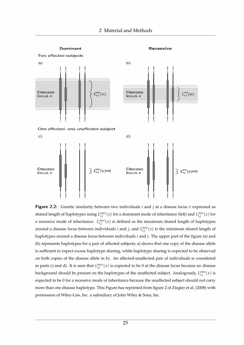
The BHS approach of using Mantel statistics on the level of haplotypes rather

than individuals might be improved by explicitly taking into account different

modes of inheritance, as an additive genetic model is implicitly assumed in the

BHS statistic. For example, while under a dominant mode of inheritance, we

cannot expect that both haplotypes derived from an affected subject carry the

causal variant (Figure 2.2a), under a recessive genetic model this is supposed

to be the case (Figure 2.2b). To formulate the problem more precisely, we are

looking for haplotype fragments that are shared on longer stretches within

patients than within controls in case of dominant or recessive modes of inheri-

tance. For this purpose the shared length between all haplotypes derived from

individual i and all haplotypes derived from individual j is computed. For ex-

ample, the shared length between the first haplotype derived from individual

22


i and the second haplotype derived from individual j at the putative disease

locus x is denoted by L(1,2)i,j (x). For a dominant mode of inheritance we suggest

to use

Lmaxi,j (x) = max{L

(1,1)i,j (x), L

(1,2)i,j (x), L

(2,1)i,j (x), L

(2,2)i,j (x)} (2.4)

as the shared length between the individuals i and j. The basis of this defini-

tion can be explained with help of the following example. Imagine that two

affected individuals i and j with two and one haplotype carrying the disease

causing mutation at locus x (Figure 2.2a). Some haplotype pairs of these indi-

viduals do not share the disease causing fragment, i.e., L(1,2)i,j (x) = 0. By taking

the maximum of the shared length of the haplotype pairs, it is ensured that the

largest haplotype fragment around the locus x is found that both individuals

have in common.

Under a recessive mode of inheritance, both haplotypes of an affected individ-

ual have to contain the disease causing mutation. This implies that all haplo-

type fragments around the locus x of two subjects should be identical (Figure

2.2b). It is thus reasonable to search for the smallest shared fragment across all

individual haplotype combinations, i.e.,

Lmini,j (x) = min{L

(1,1)i,j (x), L

(1,2)i,j (x), L

(2,1)i,j (x), L

(2,2)i,j (x)} (2.5)

Figures 2.2c and 2.2d consider an affected-unaffected pair of individuals. While

Lmaxi,j (x) is expected to be 0 at the disease locus because the unaffected subject

should not carry any disease allele, Lmini,j (x) is expected to be 0 around the dis-

ease locus for a recessive mode of inheritance because the unaffected subject

should not have more than one disease carrying haplotype.

For a pair of unaffected subjects, only random haplotype sharing is expected,

and both Lmaxi,j (x) and Lmin

i,j (x) are expected to be 0 at the disease locus in pan-

23


mictic populations. An example for the calculation of Lmaxi,j (x) and Lmin

i,j (x) is

given in Figure 2.3.

24


Figure 2.2: Genetic similarity between two individuals i and j at a disease locus x expressed as

shared length of haplotypes using Lmaxi,j (x) for a dominant mode of inheritance (left) and Lmin

i,j (x) for

a recessive mode of inheritance. Lmaxi,j (x) is defined as the maximum shared length of haplotypes

around a disease locus between individuals i and j, and Lmini,j (x) is the minimum shared length of

haplotypes around a disease locus between individuals i and j. The upper part of the figure (a) and

(b) represents haplotypes for a pair of affected subjects; a) shows that one copy of the disease allele

is sufficient to expect excess haplotype sharing, while haplotype sharing is expected to be observed

on both copies of the disease allele in b). An affected-unaffected pair of individuals is considered

in parts c) and d). It is seen that Lmaxi,j (x) is expected to be 0 at the disease locus because no disease

background should be present on the haplotypes of the unaffected subject. Analogously, Lmini,j (x) is

expected to be 0 for a recessive mode of inheritance because the unaffected subject should not carry

more than one disease haplotype. This Figure has reprinted from figure 2 of Ziegler et al. (2008) with

permission of Wiley-Liss, Inc. a subsidiary of John Wiley & Sons, Inc.

25


Figure 2.3: The shared length Lmini,j (x) for a pair of individuals i and j is given by the minimum

length over all four haplotypes surrounding the disease locus x. The dark grey blocks depict the

haplotype with the disease causing variant. For illustrative purposes, the disease is assumed to

be autosomal recessive. Lmini,j (x) is represented by the grey shaded area and equals 2. Lmax

i,j (x) is

represented by the light grey area and equals 4. This Figure has reprinted from figure 3 of Ziegler

et al. (2008) with permission of Wiley-Liss, Inc. a subsidiary of John Wiley & Sons, Inc.

26


2.1.3 Novel haplotype sharing Mantel test statistics

The genetic similarity measures Lmaxi,j (x) and Lmin

i,j (x) which are adjusted to domi-

nant and recessive modes of inheritances form the foundation of our new model-

based HS Mantel test statistics

M(d)(x) =n−1

∑i=1

n

∑j=i+1

Lmaxi,j (x)Yi,j (2.6)

and

M(r)(x) =n−1

∑i=1

n

∑j=i+1

Lmini,j (x)Yi,j. (2.7)

In this context, the term ”model-based” means that the test statistic is adapted to a

specific genetic model but not to a distributional assumption for the phenotypes and

haplotypes. For simplicity, we drop the position index x in the following. In most

applications, the underlying genetic model is unknown, and the use of a model-

based test statistic may lead to a substantial loss of power (Ziegler and Konig, 2006,

section 6.2.2). On the basis of our HS Mantel statistics and the BHS Mantel statis-

tic (Beckmann et al., 2005b), we propose two model-free max-test statistics in the

sense of Freidlin et al. (2002). To make the three test statistics M, M(d) and M(r)

comparable with respect to location and variability, we first estimated the mean and

the standard deviation of each HS statistic under the null hypothesis from permu-

tations.

Second, we standardized the test statistics using the estimated mean and standard

deviation, yielding Ms, M(d)s and M

(r)s . Specifically, let E(M) denote the empirical

expectation and SD(M) the empirical standard deviation of the HS Mantel statis-

tic, both derived by permutations, the standardized statistic is defined as (M −E(M))/SD(M). Although Mantel (1967) provided exact formulae for the mean and

27


the variance of space-time clustering statistics under permutation distributions, we

propose estimation from Monte-Carlo simulations. The first max-test statistic se-

lects the maximum of the standardized HS statistics for the additive, dominant and

recessive models so that MAX1 = max{Ms, M(d)s , M

(r)s }. The second max-test statis-

tic is linear combination of the standardized HS statistics for the additive, dominant

and recessive models and we call the linear combination the MAX2.

2.2 Assessment of statistical significance

2.2.1 Monte Carlo Permutation

For n individuals in our sample with haplotypes and phenotypes, the null hypoth-

esis of no association is equivalent to the situation that the individual haplotypes

occur independently with the phenotypes. Fundamentally we can compute the full

null distribution by computing the test statistic for all n! possible permutations of

the individual haplotypes over the phenotypes, which is not practical for n too large

due to computational limitations. However, a Monte-Carlo approach may be more

practical.

In this approach, we calculate first the statistic M at marker x based on the observed

individual haplotype and phenotype dataset. Second, we generate N replicated

datasets by randomly permuting the haplotypes shared length values among indi-

viduals and keeping the phenotype values fixed. Third, the permuted test statis-

tics M were calculated for deriving the empirical null distribution of the statistic

at marker x. The advantage of this approach was that no assumption about the

marginal distribution of the phenotypes and haplotypes had to be made, and this

approach was analogous to the one taken by Beckmann et al. (2005b). All tests con-

28


sidered were two-sided.

2.2.2 Test based on the assumption of asymptotic distribution of

haplotype sharing Mantel statistics

HS models are most commonly presented as U-statistics (Schaid et al., 2005), in-

cluding HS based on Mantel statistic (Beckmann et al., 2005a,b; Kleensang et al.,

2005; Qian, 2005). Therefore, the first test is based on the assumption that the HS

Mantel statistics are asymptotically normally distributed. The test statistics are than

constructed as

Z =M − E(M)

SD(M)(2.8)

where E(M) denotes the exact expectation and SD(M) the exact standard deviation

of M HS Mantel test statistic.

Secondly, analogously to Allen and Satten (2007b), we also develop a simple frame-

work of our and BHS Mantel statistics useful for association mapping in case-control

data for qualitative traits. This framework allows derivation of simple variance es-

timators and asymptotic distributions for HS Mantel test statistics. For the i-th of n

case-control pairs of individuals, let H1i and H0i denote case and control individu-

als hapoltypes respectively. Assume that we are comparing individuals haplotypes

having a fixed number of loci L. In this case, there are 2L possible haplotypes and

2L−1(2L + 1) possible individuals and the sharing function S(i, j) can be replaced

by a k × k matrix having (i, j)-th element S(i, j) , where k is the number of possi-

ble haplotypes or individuals for Beckmann and our forms of HS Mantel statistic

respectively. Initially assuming no phase ambiguity, we define the k-dimensional

29


vectors of cases haplotypes frequencies ρ, having j-th component

ρj =1

n ∑i=1

I[Hi1 = j], (2.9)

for j = 1, ..., k , a similar equation for π (control haplotypes frequencies) replaces Hi1

by Hi0. Then we can rewrite the mean of model-based HS Mantel test statistics as

follow.

Mx = (ρ + π)T · S · (ρ + π) (2.10)

where ρ = (1 − µ) · ρ and π = (−µ) · π and µ denotes the population mean of the

phenotype. When there is no phase ambiguity, ρ + π can be written as the mean of

independent and exchangeable random vectors

ρ + π =1

n ∑i

(ρi + πi), (2.11)

and, as such, is normally distributed, with variance-covariance matrix estimable by

the empirical variance-covariance matrix

Σ =1

n ∑i

(ρi + πi)(ρi + πi)T + (ρ + π)(ρ + π)T. (2.12)

Therefore, using Slutsky’s theorem (Serfling, 1980, section 1.5.4), the mean of model-

based HS Mantel test statistics has a mixture of independent χ2 variates, with weights

given by the eigenvalues of the matrix SΣ (Imhof, 1961). Let the rank of S be d and

the nonzero eigenvalues of SΣ be λ1, λ2, ..., λd. The first approximation to the distri-

bution of Mx is to rescale Mx by referring M′x = c−1Mx to χ2

d , where c = ∑di=1 λi/d

(Yuan and Bentler, 2007). We will use the notation

M′x ∼ χ2

d or Mx ∼ cχ2d (2.13)

30


to imply approximating the distribution of M′x by χ2

d or that of Mx by cχ2d. It is

obvious that E(M′x) = d, so that the rescaling is actually a mean correction. The

second more sophisticated correction is

Mx ∼ aχ2b, (2.14)

where a and b are determined by matching the first two moments of Mx with those

of aχ2b. Straightforward calculation leads to

a =∑

di=1 λ2

i

∑di=1 λi

and b =(∑

di=1 λi)

2

∑di=1 λ2

i

(2.15)

These approximations were originally proposed by Welch (1938) and further studied

by Satterthwaite (1941) and Box (1954). When both Σ and S can be consistently

estimated, c, a and b will be estimated as c = tr(SΣ)/d, a = tr[(SΣ)2]/tr(SΣ),

b = [tr(SΣ)]2/tr[(SΣ)2]. With these choices, the HS Mantel statistics are significant

at level α when it is larger than

cq1−α,b and aq1−α,b (2.16)

Alternatively, the p values for test statistic are

Sb(Mx/c) and Sb(Mx/a) (2.17)

where Sb is the survival function for a central χ2 distribution with b degrees of free-

dom. Finally, following Imhof (1961), we approximate this weighted χ2 distribution

using a three-moment approximation. With this choice, the HS Mantel statistics are

significant at level α when it is larger than

c1 + (q1−α,b − b)√

c2/b, (2.18)

31


where cj = ∑r λjr, b = c3

2/c23, and qβ,b is the β-th quantile of a central χ2 distribution

with b degrees of freedom, and {λr} are eigenvalues of ΣS. Alternatively, the p

value for test statistic is

Sb((Mx − c1)√

b/c2 + b). (2.19)

For our model-free HS Mantel test statistics, we also give a simple method to de-

rive the distribution for test statistics. We showed throughout this section that,

the distributions of the mean of model-based HS Mantel test statistics are normal

or a mixture of independent χ2 variates with weights given by the eigenvalues of

the matrix SΣ, which will have some cumulative distribution function Fx. Denot-

ing U1 = Fx(M(d)), U2 = Fx(M(r)) and U3 = Fx(M) we obtain the corresponding

random sample U1, U2, U3 from the standard uniform distribution. Therefore, the

probability of the order statistic U(2) = max(U1, U2, U3) of the uniform distribution,

which is equal to MAX1 HS Mantel test statistic, is a Beta random variable

U(3) ∼ B(3, 1). (2.20)

For MAX2 HS Mantel test statistic, the distribution can only be found if the distribu-

tions of the mean of model-based HS Mantel test statistics are normal as following

MAX2 ∼ N(0, 3). (2.21)

Notes on Implementation

If k, the number of all possible individuals, is very large, we may want to restrict at-

tention to a set of R individuals having non-zero or non-negligible frequency, possi-

bly with additional component corresponding to all other individuals. Suppose the

R individuals we wish to include are j1, j2, ..., jR. Let C denote a R × k or (R + 1)× k

32


matrix (the larger dimension corresponding to the situation in which minor haplo-

types are pooled), where the r-th row of C has all elements 0 except the jr-th element

which is 1; the (R + 1)-th row would have 1 in every entry except j1, j2, ..., jR. Then,

the reduced vectors of ρ and π case and control individuals haplotypes frequencies

can be written as ρ = C · ρ and π = C · π respectively, and the variance-covariance

matrix of (ρ + π) has the form Σ = CΣCT.

The asymptotic normality of (ρ + π) can also be obtained directly, thereby avoid-

ing the requirement that the k-dimensional vector (ρ − π) be normally distributed.

In our implementation, we used the R individuals having frequency Pj > n−1,

where Pj = 12n ∑i=1{I[Hi1 = j] + I[Hi1 = j]} and n is the number of case-control

pairs of individuals. All remaining (minor) individuals were pooled together and

were retained if their cumulative frequency exceeded n−1. If minor individuals are

pooled, we must define a reduced sharing matrix S that corresponds to retaining

only those elements in the rows and columns of S corresponding to individuals in

the set J = {j1, j2, ..., jR}. Further, if the last components of ρ and π correspond to

pooled minor individuals, the last row and column of S must be defined in some

way. We used

S J,R+1 = Φ−1 ∑k/∈J

S JkPk (2.22)

and

SR+1,R+1 = Φ−2 ∑k/∈J

∑k′/∈J

PkS JkPk (2.23)

Where

Φ = ∑k/∈J

Pk. (2.24)

33


All results presented in the previous section remain valid with ρ, π , Σ and S re-

placed by ρ, π, Σ and S, respectively.

2.2.3 Definition of quantile-quantile plot

Quantile-quantile plots (also called q-q plots) are used to detemie if two datasets

come from population with common distribution. In statistic, a q-q plot is a graphi-

cal method for diagnosing differences between the probability distribution of a sta-

tistical population from which a random sample has been taken and a comparison

distribution. If the population distribution is the same as the comparison distribu-

tion this approximates a straight line, especially near the center. If the quantiles of

the theoretical and data distributions agree, the plotted points fall on or near the

line y = x. If the theoretical and data distributions differ only in their location or

scale, the points on the plot fall on or near the line y = β1x + β0. The slope β0 and

intercept β1 are visual estimates of the scale and location parameters of the theoret-

ical distribution. In the case of substantial deviations from linearity, the statistician

rejects the null hypothesis of sameness.

2.3 Adaptation of haplotype sharing Mantel statistics

to missing data

So far, we assume that all haplotypes were typed for the same set of markers and

that no marker information is missing. However, this is not always the case in real

datasets. For large-scale genotyping studies, it is common for most subjects to have

some missing genetic markers, even if the missing rate per marker is low. Fur-

34


thermore, excluding subjects with missing genotypes can remove a large portion of

subjects and thereby decrease power. Therefore, we propose and compare several

approaches to deal with missing data when using HS Mantel statistic methods.

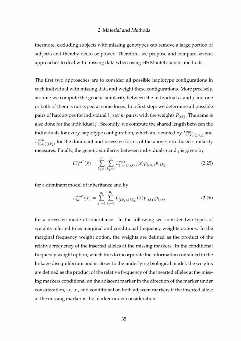
The first two approaches are to consider all possible haplotype configurations in

each individual with missing data and weight these configurations. More precisely,

assume we compute the genetic similarity between the individuals i and j and one

or both of them is not typed at some locus. In a first step, we determine all possible

pairs of haplotypes for individual i , say ni pairs, with the weights P(i,k). The same is

also done for the individual j . Secondly, we compute the shared length between the

individuals for every haplotype configuration, which are denoted by Lmax(i,k1)(j,k2)

and

Lmin(i,k1)(j,k2)

for the dominant and recessive forms of the above introduced similarity

measures. Finally, the genetic similarity between individuals i and j is given by

Lmax∗i,j (x) =

ni

∑k1=1

nj

∑k2=1

Lmax(i,k1),(j,k2)

(x)p(i,k1)p(j,k2) (2.25)

for a dominant model of inheritance and by

Lmin∗i,j (x) =

ni

∑k1=1

nj

∑k2=1

Lmin(i,k1),(j,k2)

(x)p(i,k1)p(j,k2) (2.26)

for a recessive mode of inheritance. In the following we consider two types of

weights referred to as marginal and conditional frequency weights options. In the

marginal frequency weight option, the weights are defined as the product of the

relative frequency of the inserted alleles at the missing markers. In the conditional

frequency weight option, which tries to incorporate the information contained in the

linkage disequilibrium and is closer to the underlying biological model, the weights

are defined as the product of the relative frequency of the inserted alleles at the miss-

ing markers conditional on the adjacent marker in the direction of the marker under

consideration, i.e. x , and conditional on both adjacent markers if the inserted allele

at the missing marker is the marker under consideration.

35


In the second two approaches the calculation of the shared length of two haplotpyes

is modified. We investigate two different modifications, which will be referred to as

score 1 and 2. In score 1, two haplotypes are considered as carrying different alleles

at locus, if one or both haplotypes are not typed at that marker. In score 2, they are

considered to carry the same allele at loci with missing data.

Finally, we consider fastPHASE haplotype reconstruction method. The haplotype

reconstruction package fastPHASE (Scheet and Stephens, 2006) assumes that hap-

lotypes in a population cluster into groups over short chromosome regions, and

cluster memberships are allowed to change continuously along a chromosome ac-

cording to a hidden Markov model (Rabiner, 1989). The EM algorithm is used to

estimate genetic parameters and haplotype frequencies, and unobserved haplotype

phase. For each missing genotype, the posterior mean from fastPHASE was used to

predict it.

2.4 New measure of genetic similarity of haplotype

sharing Mantel statistics

Existing varieties of HS methods assume haplotypes are known, or have been in-

ferred, an assumption that is unrealistic for genome-wide data. We therefore present

an extension of these methods that can successfully analyze genotype, rather than

haplotype, data. Such an extension was first introduced by Jung et al. (2007). The

method calculates a genetic similarity measure equal to the maximum possible hap-

lotype shared length around x , which is greater than or equal to the haplotype

shared length of (unobserved) true haplotypes.

Suppose we have data for L SNPs on each individual’s haplotypes. Let L(i) denote

36


the location (in kb) of SNP i . Let gi,j denote the genotype data for individual j at

SNP i, where gji is defined as the number of copies of the minor allele at this locus.

At each location x, our method (algorithm) calculates a similarity measure equal to

the maximum possible haplotype shared length around location x. More precisely,

suppose we are considering a pair of individuals j1 , j2 in a region centered around

SNP x on chromosome C, we define first a function f j1,j2(i) as:

f j1,j2(i) =

2 if gj1i = gj2i;

1 if∣

∣gj1i − gj2i

∣

∣ = 1;

0 if∣

∣gj1i − gj2i

∣

∣ = 2.

(2.27)

for dominant mode of inheritance, and as:

f j1,j2(i) =

2 if gj1i = gj2i;

0 if∣

∣gj1i − gj2i

∣

∣ = 1;

0 if∣

∣gj1i − gj2i

∣

∣ = 2.

(2.28)

for the recessive mode of inheritance. Secondly, to stop recording shared lengths

on a given haplotype as soon as a mismatch is found, we further define Fj1,j2(i) as

following

Fj1,j2(i) =

min{ f j1,j2(i), f j1,j2(i + 1), ..., f j1,j2(x)} if i < x;

f j1,j2(i) if i = x;

min{ f j1,j2(i), f j1,j2(i − 1), ..., f j1,j2(x)} if i > x.

(2.29)

Finally, for each pair of individuals j1 and j2 we define the similarity around x as

Sj1,j2(x), where

Sj1,j2(x) =x−1

∑i=1

Fj1,j2(i) [L(i + 1) − L(i)] +L

∑i=x+1

Fj1,j2(i) [L(i) − L(i − 1)] (2.30)

37


2.5 Case-control simulated data

For haplotype simulation, we utilized an Ancestral Recombination Graph (ARG)

based software (Hudson, 2002). The haplotypes consist of segregating loci, and

each locus represents a diallelic polymorphisms. The software operates with vari-

ables such as population size, mutation rate, recombination rate and chromosomal

length. Analogously to Beckmann et al. (2005b), we assumed random mating in

a constant effective population size 20,000 and simulated a 100,000 base pairs (bp)

region. Mutation rate per marker and generation was 5 × 10−9, and the recombina-

tion fraction between two consecutive markers was 10−9 per generation. A set also

of 10,000 haplotypes was simulated, whereas each haplotype consisted of 15 SNPs.

The minor allele frequency (MAF) was greater than 5% and the haplotype samples

were selected for a strong LD, i.e. D′> 0.7 for neighboring SNPs.

The set of 10,000 simulated haplotypes was divided into 5,000 individuals in ev-

ery single replicate; the individual haplotype pairs were randomly chosen without

replacement. We generated the disease status based on the genotype at a putative

disease locus depending on the disease models stated in Table 2.1 for all individ-

uals. The disease causing marker locus was randomly chosen for each replication.

Two disease models were considered according to the genotype penetrances and

modes of inheritance (dominant, recessive and additive mode of inheritance). Dis-

ease model I reflects a weaker complex disease model with a reduced penetrance for

the disease locus and phenocopies, whereas disease model II is closer to a Mendelian

disease with high penetrance for the disease locus. The baseline risk allows for locus

and/or allelic heterogeneity.

Case and control samples were randomly chosen from the data. For investigating

power, the sample sizes consisted of 100 to 500 case-control pairs in each replication.

Under the null hypothesis of no correlation, the disease status was randomly chosen

38


with probability 0.5. The sample consisted of 100 cases and 100 controls for each

replicate. Furthermore, we have chosen µ = 0.05 as the disease prevalence in the

population for the analysis (Beckmann et al., 2005b). The results of this simulation

were based on 1,000 independent replicate.

Table 2.1: Genotype penetrances for different disease models used in the analysis. This table has

reprinted from table 1 of Ziegler et al. (2008) with permission of Wiley-Liss, Inc. a subsidiary of John

Wiley & Sons, Inc.

Disease model I Disease model II

Genotypea Dominant Recessive Additive Dominant Recessive Additive

(1,1) 0.170 0.170 0.017 0.170 0.170 0.017

(1,2) 0.580 0.170 0.169 0.902 0.170 0.424

(2,2) 0.580 0.580 0.338 0.902 0.902 0.848

a 1: Normal allele, 2: Disease allele.

2.5.1 Haplotype estimation assessment

To study the impact of unphased haplotypes, we analyzed both the type I error

and the power using the true simulated haplotypes and the best estimate haplo-

types. The true and estimated haplotypes consisted of 15 markers. The best haplo-

type pairs for unrelated individuals were estimated using fastPHASE (Scheet and

Stephens, 2006). For the type I error analysis, the samples consisted of 100 case-

control pairs where the disease status was assigned as described before under the

null hypothesis of no correlation. For power analysis, the disease status was as-

signed as described in Table 2.1 under disease models II for dominant, recessive

and additive mode of inheritance. The sample consisted of 300 case-control pairs.

For 1,000 replicates, HS Mantel statistic methods were applied to the true simulated

haplotypes and the best estimate haplotypes.

39


2.5.2 Missing data generation

In order to evaluate the impact of allowing haplotypes with missing markers rather

than discarding them, we designed 3 patterns of missing data. In pattern 1: for

a random half of case-control pairs of simulated haplotypes, alleles were kept un-

changed, i.e. no missing data was introduced. For the remaining half of case-control

pairs, 3 markers (located at map positions 2, 7 and 12) were set as missing in the hap-

lotypes, and in addition 0, 1 or 2 markers randomly drawn from the 12 remaining

markers were also set as missing in these haplotypes according to a discrete uniform

distribution. The position of the additional missing marker(s) was also chosen ran-

domly. In pattern 2: all case-control pairs of simulated haplotypes were concerned

with 3, 4 or 5 missing markers randomly drawn among the 15 markers. In pattern

3: also all case-control pairs of simulated haplotypes were concerned with missing

data, but with 6, 7 or 8 markers randomly drawn among the 15 markers as missing.

We considered pattern 2 and 3 of missing data, in order to evaluate the impact of

different amount and distribution of missing data on power of HS Mantel statistic

methods using the five different approaches to deal with missing data.

For investigating the validity of the test statistics, the samples consisted in 100 cases

and 100 controls with an assignment of the disease status as described before. For

power analysis, the disease status was assigned as described in Table 2.1 under dis-

ease model II for a dominant, recessive and additive mode of inheritance for 300

cases and 300 controls. For each scenario, the number of replicates was 1,000.

2.5.3 Genotyping errors data generation

To evaluate the effect of genotyping errors (allele changes) in haplotypes that oc-

cur completely at random on the type I error and the power of all investigated HS

40


Mantel test statistics to detect disease gene, we define what we mean by error. In

this study, we define an error in either of the allele numbers of an individual’s geno-

type to be a change from the allele value i to i + 1 or i − 1. For the case where

i = 1, an error means that i is changed to 2, and for the case where i = 2, an er-

ror means i is changed to 1. We introduce errors randomly and independently into

the set of genotypes formed by the individual’s haplotypes in each replicate with

the same probability α. For the purpose of introducing errors, if we have N indi-

viduals, then we have 30N alleles. If the error rate is α, then the probability that

any of the 30N alleles is changed is α. We consider error rates of 1%, 5%, and 10%.

The 1% error rate is considered because Brzustowicz et al. (1993) quoted genotype

error rates of between 0.5% and 1.5% for CEPH data. The 5% error rate is consid-

ered because Brzustowicz et al. (1993) quoted genotype error rates of at least 3% by

retyping four markers in the entire CEPH panel. We consider a 10% error rate be-

cause Ehm et al. (1996) estimated error rates of more than 10% for six markers in HC

6 CEPH pedigree data. These authors applied a maximum likelihood approach to

estimate error rates. Genotype errors for each error rate in our study are generated

independently.

For investigating the validity of the test statistics, the samples consisted in 100 cases

and 100 controls with an assignment of the disease status as described before. For

power analysis, the disease status was assigned as described in Table 2.1 under dis-

ease model II for a dominant, recessive and additive mode of inheritance for 300

cases and 300 controls. For each scenario, the number of replicates was 1,000.

41


2.6 Quantitative trait data

The haplotypes data were simulated as described in section 2.5. Based on this set

of 10,000 haplotypes generated above in section 2.5 and a given quantitative trait

model, we generated random sampling. We considered the following widely used

quantitative trait model (Falconer model) at the trait locus:

Yi = α + βgi + εi (2.31)

where Yi is the trait value; α denotes the baseline risk and β the penetrances for gi;

gi (gi = a ∗ Ai + d ∗ Di) is the genetic effect due to the trait locus, Ai and Di are the

additive and dominant genotypic scores, respectively; and εi is a normal random

variable with mean 0 and variance 1 and is independent of the genotype. Ai takes

the values 1, 0, and -1, and Di takes the values 0, 1, and 0 for genotypes 2/2, 2/1

and 1/1, respectively, in which 2 is the allele corresponding to the high trait value.

The additive genetic variance attributable to the locus is σ2a = 2pq [a − (p − q) d]2,

the dominant genetic variance is σ2d = (2pqd)2, and the total genetic variance is

σ2G = σ2

a + σ2d , where p is the frequency of the allele corresponding to the high trait

value at the trait locus and q = 1 − p. The broad-sense heritability attributable to

the locus is computed by H2 = σ2G/

(

σ2G + 1

)

=(

σ2a + σ2

d

)

/(

σ2a + σ2

d + 1)

(Fisher,

1918; Schork et al., 2000).

Here, we considered the dominant genetic model (d = a), the recessive genetic

model (d = −a) and the additive genetic model (d = 0). For a given frequency

of the allele corresponding to high trait value p, and the broad sense heritability

H2, we calculated the value of a. In this thesis, we let α = 0, β = 1 and H2 =

30%. Furthermore, the overall mean is the mixture of the genotype specific means

multiplied by their respective occurrence probabilities, i.e. by µ = p2a + 2pqd +

q2(−a). To analyze the power, the sample sizes consisted of 100 to 500 individuals

42


in each replication. Under the null hypothesis of no correlation (no gene effect),

the sample sizes consisted of 100 individuals in each replication. The results of this

simulation were based on 1, 000 independent replication.

2.7 Genetic Analysis Workshop 15 data

2.7.1 Simulated data

We re-analyzed 100 replicates of simulated data provided for the Genetic Analysis

Workshop 15 Problem 3, modeled after the rheumatoid arthritis (RA) data (Miller

et al., 2007). Each replicate includes 1,500 nuclear families of size 4 (2 parents and an

affected sib pair (ASP)) and 2,000 unrelated controls. We have focused on a number

of regions, and phenotypes, motivated by the knowledge of the results. Specifically,

we look at chromosomes 6, 18, on which we expect to find signals (we analyze with

the answers known to us), and chromosome 3, on which there should be no signal.

We give details of each analysis, and present output for replicate 1 of the data to

illustrate the behavior of our methods. Then, in order to get an indication of power

of the HS Mantel test statistic methods using the new measure of genetic similarity,

we look at behavior across all 100 replicates for each of these cases. In all cases we

have used genotypes formed from the standard SNP data, (STR, and the dense SNP

map on chromosome 6, have been excluded from the analysis).

Chromosome 6: We use the full set of the cases as well as the panel of 2,000 control

samples. Parents of cases were excluded. We use RA affection status as the binary

phenotype of interest.

Chromosome 18: Here we analyzed just the case individuals. Anti-CCP level was

used as the phenotype. Cases were ranked according to anti-CCP level. Ten sub-

samples of size 200 were then formed by sampling 100 ”high” individuals with an-

43


tiCCP level = 210, and 100 ’low’ individuals with (antiCCP level ≤ 20). No signal

was seen (results not shown). However, when we restrict the analysis only to cases

with a DR status of ”3” we did uncover a signal, shown in Figure/Table below in

the results chapter.

Chromosome 3: We also wish to analyze a region in which we do not expect to find

a signal. Thus we perform an analysis of chromosome 3 in which all details are the

same as those given for chromosome 6 above.

2.7.2 Candidate region of chromosome 18q

As an application of the presented methods, with kind permission of Peter K. Gregersen

and the investigators in the North American Rheumatoid Arthritis Consortium (NARAC),

we re-analyzed the RA dataset of the NARAC provided for the Genetic Analysis

Workshop 15 (Amos et al., 2007) . The dataset comprises 460 cases and 460 controls

which were genotyped at 2,300 SNPs, covering 10 Mega bases (Mb) on chromosome

18q. Controls were recruited from a New York City population, and cases were as-

certained from multiple U.S. centers. The phenotype variable to be analyzed was

the American Rheumatoid Arthritis affection status, and the disease prevalence µ is

1% in the population (Begovich et al., 2004). All affected subjects met the standard

American College of Rheumatology criteria for affection with RA (Jawaheer et al.,

2004). The most likely pairs of haplotypes were estimated by use of fastPHASE

(Scheet and Stephens, 2006).

44


2.8 Software

The haplotypes were generated using the program ms (Hudson, 2002) (see http://h-

ome.u- chicago.edu/ rhudson1/), and fastPHASE was employed for estimating miss-

ing genotypes and reconstructing haplotypes from unphased SNP of unrelated in-

dividuals (Scheet and Stephens, 2006). All other calculations were performed with

software developed within our group available on CD attached to the thesis.

45

3 Results

3.1 Case-Control study analysis

To evaluate the feasibility of our and BHS Mantel approaches when applied to case-

control data, we analyzed both type I error and the power to map disease predis-

posing genes. The analysis was based on 1,000 replicates, and the haplotypes data

were simulated as described in section 2.5. The permutation test for significance

was performed 1,000 times. Table 3.1 gives the empirical type I error fractions for

our and BHS Mantel statistics at a nominal significance level of 5% and for a Bonfer-

roni corrected nominal significance level of α = 0.05/15. At α = 0.05, all statistics

yielded point-wise valid tests (range: 0.025-0.054), and the means of the type I errors

of the 15 SNPs ranged between 0.032 and 0.047 for the investigated test statistics.

However, the point-wise significance level 5% led to an unacceptable increase of the

relative frequency of replication with at least one false-positive (multiple tests) over

all statistics. Over all replicates, the multiple false-positive varied between 0.142

and 0.267. To adjust for multiple testing, a Bonferroni correction was applied by

dividing the point-wise significance level of 5% by the number of tests performed in

each replication. After the Bonferroni correction, all statistics led to valid multiple

types I errors fractions below 5%.

46

3 Results

Empirical power was analyzed at the nominal significance level of 0.05. Figure 3.1

shows that power increased with sample size, and it was greater for the less com-

plex disease model II. Under the dominant and the recessive mode of inheritance,

the HS Mantel statistics based on the genetic similarity measures adapted to the cor-

responding mode of inheritance, i.e. M(d) and M(r), gave the best performance, val-

idating the ideas underlying these statistics. Under a dominant inheritance pattern

the empirical power of the HS Mantel statistic for a dominant model did not exceed

65% and 85.2% for 500 case-control pairs in disease model I and II, respectively. Un-

der a recessive inheritance pattern, the empirical power of the HS Mantel statistic for

a recessive model was 75.2% and 88.7% for 500 case-control pairs in disease model I

and II, respectively. For an additive mode of inheritance, the model-free MAX1 test

statistic turned out to be the best. Even under the dominant and recessive genetic

mode of inheritances the max-test showed reasonable power compared to the best

performing HS Mantel statistic.

If the model is not specified correctly, these tests adopting the mode of inheritance

perform poorly, while the BHS statistic is stable in these cases. Our novel max-

test HS Mantel statistic outperformed the BHS statistic based on an additive genetic

model proposed by Beckmann et al. (2005b) in all considered scenarios. Overall, we

conclude that the max-test is superior to the single model-based test statistics if the

mode of inheritance is unknown.

47

3 Results

Figure 3.1: Empirical power of the HS Mantel statistic adapted to a dominant and recessive

mode of inheritance M(d) [×] and M(r) [�] as well as the HS Mantel statistic suggested by Beck-

mann M [+] and the model-free MAX1 [•] and MAX2 [�] statistics based on 1,000 replicates for

different disease models of binary trait data. The results under a dominant, recessive and addi-

tive mode of inheritance are given, respectively, in the figures a and b, c and d, and e and f. All

statistics were evaluated at nominal significance level of 5%. This figure has been adopted from

figure 4 of Ziegler et al. (2008) with permission of Wiley-Liss, Inc. a subsidiary of John Wiley &

Sons, Inc.

48

3 Results

Table 3.1: Empirical type I error of the HS Mantel statistics at nominal significance levels of 5%

and 0.3% based on 1,000 replicates of binary trait data, . The samples consisted of 100 cases and

100 controls. This table has been adopted from table II of Ziegler et al. (2008) with permission of

Wiley-Liss, Inc. a subsidiary of John Wiley & Sons, Inc.

α = 0.05 α = 0.003c

Method Pointwisea Multipleb Pointwisea Multipleb

M(d)(x) 0.039 (0.032-0.050) 0.142 0.002 (0.001-0.004) 0.013

M(r)(x) 0.047 (0.041-0.054) 0.267 0.002 (0.000-0.004) 0.014

M(x) 0.040 (0.032-0.045) 0.198 0.002 (0.000-0.006) 0.017

MAX1 0.032 (0.025-0.038) 0.162 0.002 (0.000-0.005) 0.017

MAX2 0.037 (0.027-0.043) 0.193 0.002 (0.000-0.006) 0.018

a Mean type I error for 15 markers, minimum and maximum are given in brackets.

b Relative frequency of replicates with at least one false-positive.

c Bonferroni correction for multiple testing: p < 0.05/15 = 0.003.

Table 3.2 shows the estimated Pearson product-moment correlation coefficients of

the three standardized HS test statistics M, M(d) and M(r) over all replicates for

disease model II and 300 case-control pairs per replicate. The correlation is strong

between M, and M(d) and between M and M(r) for all models considered. It is weak

between M(d) and M(r) for dominant and additive genetic models.

3.1.1 Linkage disequilibrium pattern within the gene

To investigate our and BHS Mantel statistics more, we examine the influence of

weak LD of the disease allele with a marker allele (or equivalently a haplotype).

The analysis was based on 1,000 replicates, and the haplotypes data were simulated

as described in section 2.5. However, the mutation rate per marker was 5 × 10−9

per generation, and the recombination rate between two consecutive markers was

49

3 Results

Table 3.2: Pearson product-moment correlation coefficients over all replicates for true haplo-

types of the standardized HS Mantel type test statistics and disease model II. Each replicate con-

sisted of 300 cases and 300 controls. This table has reprinted from table IV of Ziegler et al. (2008)

with permission of Wiley-Liss, Inc. a subsidiary of John Wiley & Sons, Inc..

Genetic model M(d)(x) M(r)(x)

Dominant M(d)(x) 1.00

M(r)(x) 0.01 1.00

M(x) 0.85 0.52

Recessive M(d)(x) 1.00

M(r)(x) 0.69 1.00

M(x) 0.91 0.91

Additive M(d)(x) 1.00

M(r)(x) 0.09 1.00

M(x) 0.70 0.76

50

3 Results

10−7 per generation for simulating datasets with weak LD pattern, i.e. D′< 0.50 for

consecutive SNPs. The sample consisted of 300 cases and 300 controls.

Table 3.3 gives the empirical type I error fractions for our and BHS Mantel statistics

at a nominal significance level of 5% and for a Bonferroni corrected nominal signifi-

cance level of α = 0.05/15 = 0.003. The results show that, the nominal Type I error

rate is within the confidence range of the observed Type I errors. At α = 0.05, all

test statistics yielded point-wise valid tests (range: 0.020-0.050), and the means of

the type I errors of the 15 SNPs ranged between 0.028 and 0.044 for the investigated

test statistics. However, the point-wise significance level 5% led to an unaccept-

able increase of the relative frequency of replicates with at least one false-positive

(multiple tests) over all statistics. Over all replicates, the multiple false-positive var-

ied between 0.175 and 0.260. To adjust for multiple testing, a Bonferroni correction

was applied by dividing the point-wise significance level of 5% by the number of

tests performed in each replication. After the Bonferroni correction, all statistics led

to valid multiple types I errors fractions below 5%. The investigate test statistics

showed slightly higher type I errors (multiple tests) compared to the results for the

case of haplotypes with more stronger LD pattern (D′> 0.70) (Table 3.1).

51

3 Results

Table 3.3: Empirical type I error of the HS Mantel statistics at nominal significance levels of 5%

and 0.3% based on 1,000 replicates of simulating datasets with weak LD pattern (D′< 0.50). The

samples consisted of 100 cases and 100 controls.

α = 0.05 α = 0.003c


M(d)(x) 0.037 (0.031-0.043) 0.186 0.002 (0.000-0.005) 0.013

M(r)(x) 0.044 (0.036-0.050) 0.318 0.003 (0.000-0.005) 0.030

M(x) 0.040 (0.034-0.047) 0.260 0.001 (0.000-0.003) 0.029

MAX1 0.028 (0.020-0.035) 0.175 0.002 (0.000-0.003) 0.019

MAX2 0.035 (0.028-0.045) 0.215 0.003 (0.000-0.005) 0.024




All statistics showed great loss of power when haplotypes with weak LD were used

compared to the results for the case of haplotypes with more stronger LD pattern

(D′> 0.70) (Tables 3.4). Our model-based and model-free HS Mantel statistics

clearly had higher power for both weaker and stronger haplotypes LD pattern com-

pared to BHS Mantel statistic.

3.1.2 True haplotypes versus best estimates

In practical applications haplotypes determined with laboratory methods are rarely

available. Therefore, one often has to rely on haplotypes that were inferred form

genotypes. Using best estimate haplotypes instead of the true ones we empirically

determined the type I error of the different HS Mantel statistics at a nominal sig-

nificance level of 5% and for a Bonferroni-corrected nominal significance level of

α = 0.05/15 = 0.003. The results of this investigation can be found in Table 3.5. At a

52

3 Results

Table 3.4: Empirical powers of the HS Mantel statistics at nominal significance levels of 5%

based on 1,000 replicates under disease model II of simulating datasets with weak or strong LD

patterns. The samples consisted of 300 cases and 300 controls data.

Genetic model LD M(d)(x) M(r)(x) M(x) MAX1 MAX2

Dominant < 0.50 0.42 0.09 0.30 0.37 0.34

> 0.70 0.78 0.17 0.60 0.75 0.70

Recessive < 0.50 0.36 0.38 0.38 0.39 0.38

> 0.70 0.65 0.82 0.77 0.79 0.77

Additive < 0.50 0.84 0.33 0.45 0.73 0.69

> 0.70 0.95 0.73 0.82 0.98 0.96

significance of level 5%, all statistics yielded point-wise valid tests. The type I error

of the single markers varied between 0.023 and 0.064. The means of the type I errors

of the 15 SNPs ranged between 0.034 and 0.049 for the investigated test statistics.

Applying a Bonferroni correction the empirical multiple type I error was lower that

5% for all investigated test statistics. M(d), M, MAX1 and MAX2 revealed slightly

higher type I errors compared to the case of true haplotypes (Tables 3.1).

All statistics showed slight loss of power when best estimate haplotypes were used

compared to the results for the case of true haplotype (Table 3.6). Our model-based

and model-free HS Mantel statistics clearly had higher power for both true and es-

timated haplotypes when compared to the BHS Mantel statistic.

53

3 Results

Table 3.5: Empirical type I error of the HS Mantel type test statistics at nominal significance

levels of 5% and 0.3% based on 1,000 replicates when best estimate haplotypes are used. The

samples consisted of 100 cases and 100 controls. This table has been adopted from table II of

Ziegler et al. (2008) with permission of Wiley-Liss, Inc. a subsidiary of John Wiley & Sons, Inc.

α = 0.05 α = 0.003c


M(d)(x) 0.048 (0.041-0.064) 0.178 0.002 (0.001-0.006) 0.010

M(r)(x) 0.045 (0.035-0.054) 0.263 0.002 (0.000-0.007) 0.020

M(x) 0.049 (0.037-0.063) 0.236 0.002 (0.000-0.006) 0.020

MAX1 0.034 (0.023-0.047) 0.186 0.002 (0.000-0.006) 0.015

MAX2 0.040 (0.033-0.052) 0.198 0.003 (0.000-0.007) 0.021




Table 3.6: Empirical power of the HS Mantel type test statistics at a nominal significance level

of 5% based on 1,000 replicates for true haplotypes (true), and best estimate haplotypes (complete

estimated) under disease model II. The samples consisted of 300 cases and 300 controls. This

table has been adopted from table III of Ziegler et al. (2008) with permission of Wiley-Liss, Inc. a

subsidiary of John Wiley & Sons, Inc.

Genetic model Haplotypes M(d)(x) M(r)(x) M(x) MAX1 MAX2

Dominant True 0.78 0.17 0.60 0.75 0.70

Complete estimated 0.75 0.15 0.58 0.72 0.67

Recessive True 0.65 0.82 0.77 0.79 0.77


Additive True 0.95 0.73 0.82 0.98 0.96


54

3 Results

3.1.3 Missing data analysis

In these former applications of our and BHS Mantel statistics, haplotypes of indi-

viduals were available. Furthermore, all the individuals were typed for the same set

of markers. The same information was thus available for all the haplotypes used in

the analysis. However, these conditions may not be met in the real data, so that a

varying amount of information is available from one haplotype to another. There-

fore, the impacts of five different approaches, regarding missing data, on our and

BHS Mantel statistics are evaluated. We empirically determined the type I error and

the power. The genetic data were simulated as described in subsection 2.5.2.

Using the five different approaches, we empirically determined the type I error for

the HS Mantel statistics at a nominal significance level of 5% and for a Bonferroni-

corrected nominal significance level of α = 0.05/15 = 0.003. At α = 0.05, all ap-

proaches yielded point-wise valid tests for all statistics (Table 3.7). The type I error

of the single markers ranged between 0.023 and 0.064, and the means of the type I

errors of the 15 SNPs ranged from 0.030 to 0.050 for the investigated test statistics.

Applying a Bonferroni correction, the empirical multiple type I error was lower that

5% for all investigated test statistics. Using fastPHASE approach for the best esti-

mate of incomplete individual haplotypes, almost all HS Mantel statistics revealed

slightly higher type I errors compared to the results in the case when the other ap-

proaches were used.

In table 3.8, as expected there was a slight loss of power in the case of missing geno-

types compared with the case of perfectly known and the best estimated haplotypes

(Table 3.6). Under a dominant inheritance pattern the empirical power was 73% for

the dominant model using fastPHASE haplotype reconstruction method. Under a

recessive inheritance pattern, the empirical power of the HS Mantel statistic for a

recessive model was 72% using all possible haplotype configurations with condi-

55

3 Results

tional frequency weight. For an additive mode of inheritance, the model-free statis-

tic MAX1 turned out to be the best with power of 92% using fastPHASE haplotype

reconstruction method.

Finally, table 3.9 shows the sensitivity of the adaptation approaches of missing data

to the level and the distribution of missing data. For different amount of missing

data, which entirely completely randomly distributed as described in pattern 2 and

3 of missing data as described in subsection 2.5.2, the power of all investigated test

statistics decreases when the amount of missing data increases. However, the ad-

vantage of fastPHASE approach is maintained for all HS Mantel test statistics.

56

3 Results

Table 3.7: Empirical type I error of the HS Mantel statistics at nominal significance level of 5%

and 0.3% based on 1,000 replicates when the five different approaches to deal with incomplete

individual haplotypes are used. The samples consisted of 100 cases and 100 controls.

α = 0.05 α = 0.003c

Method Analysis Pointwisea Multipleb Pointwisea Multipleb

M(d)(x) Marginal-weight 0.041 (0.037-0.049) 0.159 0.002 (0.001-0.003) 0.013

Conditional-weight 0.038 (0.034-0.042) 0.185 0.001 (0.001-0.002) 0.012

Score1 0.030 (0.026-0.035) 0.252 0.001 (0.001-0.002) 0.018

Score2 0.042 (0.039-0.045) 0.138 0.001 (0.001-0.002) 0.007

fastPHASE 0.049 (0.040-0.064) 0.196 0.001 (0.000-0.006) 0.015

M(r)(x) Marginal-weight 0.037 (0.029-0.045) 0.224 0.002 (0.000-0.004) 0.020


Score1 0.036 (0.023-0.042) 0.298 0.002 (0.000-0.003) 0.020

Score2 0.040 (0.031-0.047) 0.224 0.002 (0.001-0.005) 0.019

fastPHASE 0.047 (0.036-0.057) 0.278 0.002 (0.001-0.007) 0.020

M(x) Marginal-weight 0.041 (0.032-0.052) 0.192 0.002 (0.001-0.003) 0.017


Score1 0.040 (0.030-0.057) 0.120 0.002 (0.000-0.004) 0.007

Score2 0.041 (0.031-0.050) 0.202 0.002 (0.001-0.004) 0.017

fastPHASE 0.050 (0.040-0.062) 0.233 0.002 (0.000-0.007) 0.021

MAX1 Marginal-weight 0.039 (0.035-0.046) 0.226 0.002 (0.000-0.004) 0.018


Score1 0.035 (0.027-0.042) 0.272 0.001 (0.000-0.003) 0.017

Score2 0.043 (0.034-0.046) 0.201 0.002 (0.001-0.004) 0.017

fastPHASE 0.036 (0.025-0.048) 0.231 0.002 (0.001-0.005) 0.017

MAX2 Marginal-weight 0.040 (0.037-0.048) 0.210 0.002 (0.000-0.004) 0.017


Score1 0.039 (0.032-0.045) 0.287 0.001 (0.000-0.005) 0.017

Score2 0.044 (0.034-0.050) 0.240 0.002 (0.001-0.005) 0.017

fastPHASE 0.038 (0.032-0.052) 0.267 0.002 (0.000-0.004) 0.017




57

3 Results

Table 3.8: Empirical power of the HS Mantel statistics at nominal significance level of 5% based

on 1,000 replicates when the five different approaches to deal with incomplete individual haplo-

types are used under disease model II. Missing data pattern 1. The samples of haplotypes con-

sisted of 300 cases and 300 controls.

Genetic model Analysis M(d)(x) M(r)(x) M(x) MAX1 MAX2

Dominant Marginal-weight 0.61 0.15 0.46 0.56 0.54

Conditional-weight 0.65 0.16 0.48 0.60 0.56

Score1 0.37 0.13 0.25 0.38 0.35

Score2 0.64 0.16 0.45 0.57 0.53

fastPHASE 0.73 0.21 0.53 0.69 0.66

Recessive Marginal-weight 0.46 0.67 0.64 0.64 0.64


Score1 0.09 0.63 0.57 0.62 0.60

Score2 0.44 0.71 0.68 0.68 0.68

fastPHASE 0.51 0.68 0.64 0.65 0.64

Additive Marginal-weight 0.82 0.59 0.75 0.88 0.85


Score1 0.45 0.58 0.58 0.69 0.67

Score2 0.88 0.64 0.77 0.90 0.88

fastPHASE 0.90 0.64 0.78 0.92 0.91

58

3 Results

Table 3.9: Empirical power of the HS Mantel statistics at nominal significance level of 5% based

on 1,000 replicates when the five different approaches to deal with incomplete individual haplo-

types are used under disease model II. Missing data patterns 2 and 3. The samples of haplotypes

consisted of 300 cases and 300 controls.

M(d)(x) M(r)(x) M(x) MAX1 MAX2

Genetic model Analysis 2 3 2 3 2 3 2 3 2 3

Dominant Marginal-weight 0.56 0.38 0.13 0.09 0.40 0.31 0.45 0.19 0.43 0.17

Conditional-weight 0.60 0.33 0.14 0.07 0.43 0.26 0.40 0.32 0.38 0.29

Score1 0.33 0.15 0.12 0.06 0.21 0.09 0.29 0.13 0.25 0.11

Score2 0.62 0.56 0.10 0.07 0.42 0.38 0.55 0.48 0.53 0.45

fastPHASE 0.70 0.65 0.18 0.12 0.51 0.47 0.66 0.59 0.64 0.57

Recessive Marginal-weight 0.44 0.16 0.60 0.52 0.57 0.48 0.56 0.49 0.55 0.48


Score1 0.12 0.05 0.59 0.57 0.50 0.29 0.58 0.55 0.57 0.54

Score2 0.38 0.24 0.65 0.62 0.63 0.55 0.60 0.56 0.60 0.55

fastPHASE 0.48 0.28 0.60 0.59 0.58 0.51 0.55 0.49 0.53 0.48

Additive Marginal-weight 0.72 0.30 0.51 0.35 0.61 0.45 0.76 0.54 0.73 0.50


Score1 0.30 0.16 0.53 0.44 0.41 0.23 0.54 0.47 0.52 0.46

Score2 0.80 0.75 0.58 0.51 0.75 0.63 0.82 0.78 0.78 0.75

fastPHASE 0.84 0.78 0.57 0.51 0.76 0.64 0.85 0.80 0.84 0.80

3.1.4 Genotyping errors data analysis

To our knowledge, no work has been done in considering the effect of genotyping

errors on the HS Mantel test statistics. In this subsection, therefore, we evaluate the

effect of genotyping errors (allele changes) in haplotypes that occur completely at

59

3 Results

random on the type I error and the power of all investigated HS Mantel tset statis-

tics. The haplotypic data were simulated as described in subsection 2.5.3.

In table 3.10, we empirically determined the type I error of our and BHS Mantel

statistics at a nominal significance level of 5% and for a Bonferroni-corrected nom-

inal significance level of α = 0.05/15 = 0.003. At a significance of level 5%, all

statistics showed reasonable and valid type I error for the 3 different genotyping

error rates. The type I error of the single markers ranged between 0.021 and 0.057,

and the means of the type I errors of the 15 SNPs ranged from 0.033 to 0.049 for the

investigated test statistics. Applying a Bonferroni correction, the empirical multiple

type I error was lower that 5% for all investigated test statistics. Furthermore, the

results from this table indicate that there is no effect of random genotyping errors in

haplotyoes on the type I error of the test statistics.

Empirical power was analyzed at the nominal significance level of 0.05. Table 3.11

shows that there is a definite loss of power to detect disease gene with all test statis-

tics when errors are introduced. The power loss increases as the error rate increases.

Comparing to the data as given (no errors), the maximum loss of powers to detect

disease gene, using dominant HS Mantel statistic are 3%, 5%, and 11% for error rates

1%, 5%, and 10%, respectively. For recessive HS Mantel statistic, we observe maxi-

mum power losses of 2%, 6%, and 10% for error rates 1%, 5%, and 10%, respectively.

We also observe maximum power losses for BHS Mantel statistic of 1%, 5%, and

11% for error rates 1%, 5%, and 10%, respectively. For MAX1 model-free HS Mantel

statistic, we observe maximum power losses of 3%, 5%, and 11% for error rates 1%,

5%, and 10%, respectively. For MAX2 model-free HS Mantel statistic, we observe

maximum power losses of 2%, 5%, and 11% for error rates 1%, 5%, and 10%, re-

spectively. The results from this table indicate that, there might be a maximal loss of

power for error rate between 5% and 10%. We therefore recommend that researchers

maintain error rates of less than 5% in their genotype data, particularly when using

60

3 Results

the HS Mantel statistics for detect disease gene.

61

3 Results

Table 3.10: Empirical type I error of HS Mantel statistics at nominal significance levels of 5%

and 0.3% based on 1,000 replicates when three different rates of genotyping errors are used. The

samples consisted of 100 cases and 100 controls.

α = 0.05 α = 0.003c

Method Analysis Pointwisea Multipleb Pointwisea Multipleb

M(d)(x) 1% 0.043(0.031-0.054) 0.162 0.002(0.001-0.006) 0.010

5% 0.047(0.034-0.056) 0.197 0.002(0.001-0.005) 0.009

10% 0.044(0.036-0.052) 0.207 0.002(0.001-0.004) 0.014

M(r)(x) 1% 0.049(0.041-0.057) 0.285 0.003(0.000-0.006) 0.022

5% 0.046(0.032-0.055) 0.268 0.004(0.001-0.008) 0.026

10% 0.045(0.035-0.057) 0.302 0.003(0.000-0.006) 0.022

M(x) 1% 0.041(0.031-0.047) 0.207 0.002(0.000-0.004) 0.013

5% 0.045(0.037-0.050) 0.230 0.002(0.001-0.004) 0.016

10% 0.042(0.036-0.048) 0.236 0.003(0.000-0.005) 0.021

MAX1 1% 0.035(0.025-0.048) 0.179 0.002(0.000-0.005) 0.015

5% 0.034(0.025-0.044) 0.193 0.003(0.000-0.005) 0.019

10% 0.033(0.021-0.041) 0.205 0.002(0.000-0.004) 0.016

MAX2 1% 0.039(0.028-0.052) 0.198 0.002(0.000-0.005) 0.017

5% 0.037(0.027-0.050) 0.211 0.002(0.000-0.005) 0.021

10% 0.035(0.025-0.048) 0.234 0.002(0.001-0.005) 0.017




62

3 Results

Table 3.11: Empirical Power of the HS Mantel statistics at nominal significance level of 5%

based on 1,000 replicates when three different rates of genotyping errors are used under disease

model II. The samples consisted of 300 cases and 300 controls.

Genetic model Analysis M(d)(x) M(r)(x) M(x) MAX1 MAX2

Dominant 0% (no errors) 0.78 0.17 0.60 0.75 0.70

1% 0.76 0.15 0.59 0.74 0.68

5% 0.73 0.12 0.56 0.72 0.65

10% 0.68 0.09 0.51 0.67 0.61

Recessive 0% (no errors) 0.65 0.82 0.77 0.79 0.77

1% 0.63 0.81 0.76 0.78 0.76

5% 0.60 0.78 0.73 0.77 0.74

10% 0.54 0.75 0.69 0.71 0.67

Additive 0% (no errors) 0.95 0.73 0.82 0.98 0.96

1% 0.92 0.71 0.81 0.95 0.94

5% 0.90 0.67 0.77 0.93 0.91

10% 0.85 0.63 0.71 0.87 0.85

3.2 Quantitative trait data analysis

In order to evaluate the performance of HS Mantel test statistics in presence of

quantitative trait data, we analyzed the type I error and the power. The simu-

lated datasets were carried out as described in section 2.6, where the disease causing

marker locus was chosen by random for each replicate. The analysis was based on

1,000 replicates. The permutation test for significance was performed 1,000 times.

For the application of the HS Mantel statistics to quantitative traits, we propose

the mean corrected product of phenotypes, Yi,j = (Yi − µ)(Yj − µ), as measure of

63

3 Results

phenotypic similarity. Here, Yi and Yj were given by the widely used quantitative

trait model (Equation 2.31, section 2.6) for individuals i and j, respectively, with

µ = p2a + 2pqd + q2(−a) denoting the overall mean of equation 2.31.

The point-wise significance level 5% was satisfying for all investigated HS Mantel

test statistics (Table 3.12). The empirical type I error of the single markers varied

between 0.034 and 0.064. The means of the type I errors of the 15 SNPs ranged

between 0.040 and 0.053 for the investigated test statistics. Applying a Bonferroni

correction the empirical multiple type I error was lower that 5% for all test statistics.

The results of all investigated test statistics showed slightly inflated error compared

to the results in the case where we used the binary trait data (Table 3.1).

For power analysis, figure 3.2 presents the results for the power comparison be-

tween all investigated HS Mantel statistics methods at significance level 5%. The

statistics give better result for quantitative traits analysis than binary traits analysis

(Figures 3.1 and 3.2). Under a dominant inheritance pattern, the empirical powers

of any of the statistics were 70% and 86% or more for only 100 case-control pairs in

disease model I and II, respectively. Under a recessive inheritance pattern, the em-

pirical powers of any of the statistics exceed 81% and 85% for only 100 case-control

pairs in disease model I and II, respectively. For an additive mode of inheritance,

the empirical powers of any of the statistics exceed 95% and 97% for only 100 case-

control pairs in disease model I and II, respectively. Furthermore, there is slightly

different in power between the investigated HS Mantel statistics for quantitative

traits analysis.

64

3 Results

Figure 3.2: Empirical power of the HS Mantel statistics adapted to a dominant and recessive

mode of inheritance M(d) [×] and M(r) [�] as well as the HS Mantel statistic suggested by Beck-

mann M [+] and the model-free MAX1 [•] and MAX2 [�] statistics based on 1,000 replicates for

different disease model of quantitative trait data. The results under a dominant, recessive and

additive mode of inheritance are given in the figures a and b, c and d, and e and f. All statistics

were evaluated at nominal significance level of 5%.

65

3 Results

Table 3.12: Empirical type I error of the HS Mantel statistics at nominal significance levels of

5% and 0.3% based on 1,000 replicates of quantitative trait data. The samples consisted of 100

cases and 100 controls.

α = 0.05 α = 0.003c


M(d)(x) 0.053 (0.045-0.064) 0.162 0.002 (0.001-0.004) 0.007

M(r)(x) 0.046 (0.039-0.063) 0.263 0.001 (0.000-0.004) 0.018

M(x) 0.051 (0.046-0.060) 0.196 0.003 (0.001-0.005) 0.016

MAX1 0.040 (0.035-0.057) 0.187 0.002 (0.000-0.005) 0.018

MAX2 0.043 (0.034-0.059) 0.210 0.002 (0.000-0.006) 0.018




3.3 Comparison of different assumption of asymptotic

distribution for haplotype sharing Mantel test

statistics

In this section results are presented for the HS Mantel test statistics using haplo-

type information for gene mapping as proposed in section 2.5. The assumption of

asymptotic distribution will be analyzed using quantile-quantile plot method (see

section 2.2).

The sample consisted of 100 cases and 100 controls for 1000 replicates. The disease

model was the model under the null hypothesis. For the results here, SNP 4 was

chosen as the disease causing locus. Results are comparable to the cases where other

loci were chosen as the disease causing variant.

66

3 Results

3.3.1 Results of model-based haplotype sharing Mantel test

statistics

Form figure 3.3, we can not reject the assumption of normality for all model-based

HS Mantel test statistics presented. To test for the assumption of asymptotic chi-

square distribution, figure 3.4 showed the quantile-quantile plots for random sam-

ples of model-based (dominant, recessive and additive) HS Mantel test statistics

using three different approximates of χ2 distributions. Plots a, d and g indicate that

there is no major discrepancy between the proposed distribution cχ2d and the corre-

sponding empirical distribution of the statistics. However, plots b, e and h and c,

f and i indicate that the major discrepancy between the proposed distributions aχ2b

and c1 + (χ2b − b)

√c2/b and the corresponding empirical distribution of the statis-

tics occurs almost always on the right tail. Furthermore, in all plots the theoretical

and data distributions differ only in their location.

67

3 Results

Figure 3.3: A normal quantile-quantile plots for random samples of model-based (a) dominant,

(b) recessive and (c) additive HS Mantel test statistics.

68

3 Results

Figure 3.4: A chi-square quantile-quantile plots for random samples of model-based (domi-

nant, recessive and additive) HS Mantel test statistics using different approximate of χ2 distribu-

tion weights, in (a, d and g) we used cχ2d approximation, in (b, e and h) we used aχ2

b approximation,

and in (c, f and i) we used c1 + (χ2b − b)

√c2/b approximation.

69

3 Results

3.3.2 Results of model-free haplotype sharing Mantel test

statistics

For our model-free HS Mantel test statistics, we also give simple methods to derive

the distribution for test statistics. We showed throughout this section in figure 3.3

that, the distributions of the mean of model-based HS Mantel test statistics are nor-

mal, which will have cumulative distribution function Fx. Denoting U1 = Fx(M(d)),

U2 = Fx(M(r)) and U3 = Fx(M), we obtain the corresponding random sample

U1, U2, U3 from the standard uniform distribution. Therefore, figure 3.5a showed

that the probability of the order statistic U(3) = max(U1, U2, U3) of the uniform

distribution, which is equal to MAX1 HS Mantel test statistic, is a Beta random vari-

able with parameters α = 3 and β = 1 using the quantile-quantile plot method.

For MAX2 HS Mantel test statistic, figure 3.5b showed that the probability of the

statistic is normal random variable with mean 0 and variance 3.

Figure 3.5: A beta quantile-quantile plots for random samples of model-free (a) MAX1 and (b)

MAX2 HS Mantel test statistic.

70

3 Results

3.4 Analysis of the new measure of genetic similarity of

haplotype sharing Mantel statistics

This new measure of genetic similarity, in section 2.4, of HS Mantel statistics pro-

cedure results in a p-value for each SNP. A traditional way to determine these p-

values is to use a permutation scheme (see subsection 2.2.1). For Genetic Analysis

Workshop 15 simulated datasets of interest, such a scheme is computationally inten-

sive method to employ especially for chromosome 6 datasets which would require

a larger permutation test. Thus, we present statistical test based on the assump-

tion of asymptotical normality. We present output for 100 replicates of the Genetic

Analysis Workshop 15 simulated dataset to illuststrate the behavior of the methods.

Then in order to get an indication of power of the methods, we look also at the

mean distance between the trait locus and the SNP with the smallest p-value. The

results were compared to the results where we use the individual haplotypes. The

data were derived from the Genetic Analysis Workshop 15 simulated dataset as de-

scribed in subsection 2.7.1. For each analysis of given chromosomes (3, 6 and 18), for

a particular phenotype of interest, we construct datasets consisting of 100 case and

100 control (sampling without replacement from each replicate). The definition of

case and control depends on the phenotype of interest. We analyze each of these 100

dataset, record the p-value for each locus in each analysis, and report the average

p-value across the 100 analyses as the final score for that locus.

In figure 3.6, we show illustrative results for chromosomes 6, 18 and 3 (top-to-

bottom). We see clear signal (i.e. peaks) on chromosome 6 although only one signal

is detected. On chromosome 18 the signal is much less clear. In order to assess

power we present results across all 100 replicates in table 3.13. We report SNP with

smallest negative log10 p-value observed over the 100 replicates, as well as the dis-

tance between the SNP with the smallest p-value and the trait locus. The former is

71

3 Results

an indication of significance of results; the latter is an indication of accuracy. We see

that for chromosome 6 p-values is very small and SNP with the smallest p-value is

very close to the functional locus. The result for chromosome 18 is less clear the p-

value is not particularly small, but it is interesting to note that the smallest p-value

(i.e. highest negative log10 p-value) is also obtained very close to the correct lo-

cation. Compared to the results of HS Mental statistics with respect to haplotype

assignment, the peaks are slightly less pronounced. Finally, as we expect there is no

signal on chromosome 3.

72

3 Results

Figure 3.6: Results of chromosomes 6, 18 and 3 (top-to-bottom) using the HS Mantel statistics

adapted to a dominant and recessive mode of inheritance M(d) [×] and M(r) [�] as well as the HS

Mantel statistic suggested by Beckmann M [+] and the model-free statistics MAX1 [•] and MAX2

[�]. The results under a genotype and haplotype measure of genetic similarity are given in the

figures a , c and e, and b, d and f.

73

3 Results

Table 3.13: Summary results across all 100 replicates for chromosomes 3, 6 and 18. Results

show the marker corresponding to the small p-value and the location of these markers as well as

the distance between the functional locus and the marker corresponding to the small p-value.

Mean

distance

from true

-Log10(p-value) locus (bp)

Analysis Chr. Locus Location (bp) M(d)(x) M(r)(x) M(x) MAX1 MAX2

Genotype 3 NA NA 0.44 0.52 - - - NA

6 153 32499465 15.9 33.6 - - - 14,817

18 269 66048927 0.38 1.60 - - - -20,911

Haplotype 3 NA NA 0.44 0.40 0.42 0.43 0.42 NA

6 153 32499465 26.4 35.5 32.7 34.6 33.2 14,817

18 269 66048927 0.55 2.45 1.91 2.04 1.98 -20,911

3.5 Analysis of the chromosome 18q candidate region

for rheumatoid arthritis

The analyses of the RA case-control data were performed in two steps. We first

analyzed all SNPs jointly, estimated empirical p-values by 1,000 permutations and

defined interesting regions if more than three neighboring SNPs showed empirical

p-values< 0.05 (Figure 3.7). For these regions obtained in the first step of analy-

sis, we increased the number of permutations to 10,000. In this second step, we

discarded isolated markers with p < 0.005. This led to the identification of three

regions containing six known genes according to NCBI built 36.2, namely PMIP1,

MC4R, PIGN, KIAA1468, TNFRSF11A and ZCCHC2 (Table 3.14).

74

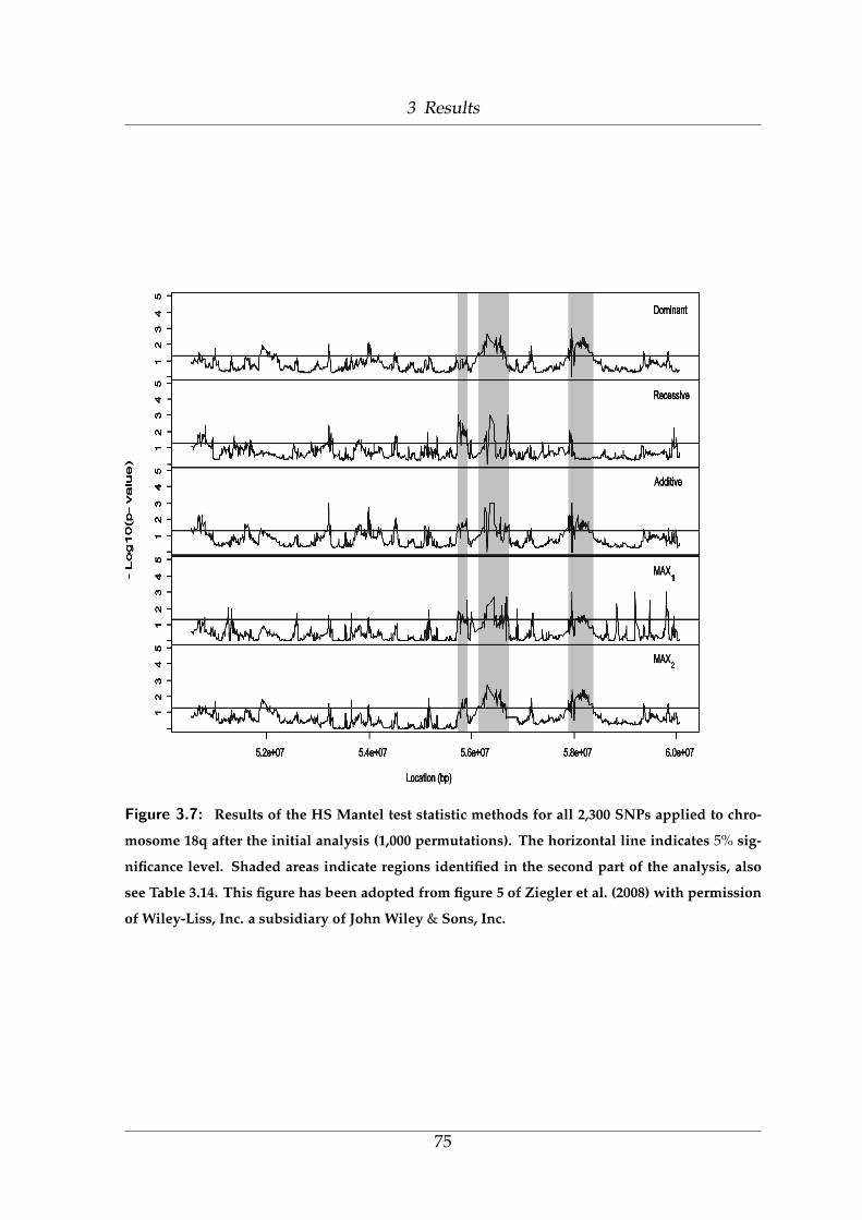
3 Results

Figure 3.7: Results of the HS Mantel test statistic methods for all 2,300 SNPs applied to chro-

mosome 18q after the initial analysis (1,000 permutations). The horizontal line indicates 5% sig-

nificance level. Shaded areas indicate regions identified in the second part of the analysis, also

see Table 3.14. This figure has been adopted from figure 5 of Ziegler et al. (2008) with permission

of Wiley-Liss, Inc. a subsidiary of John Wiley & Sons, Inc.

75

3 Results

Table 3.14: Selected regions on chromosome 18q after the second step of analysis (10,000 per-

mutations). This table has been adopted from table V of Ziegler et al. (2008) with permission of

Wiley-Liss, Inc. a subsidiary of John Wiley & Sons, Inc.

Regionsa SNPs Locations (bp) Known genesb Test statistics

1 rs1975145-rs4940711 55,716,153-55,920,566 PMIP1 M(r)(x)

2 rs4940736-rs3760559 56,130,405-56,727,645 MC4R M(d)(x)

M(r)(x), M(x)

MAX1, MAX2

3 rs1943232-rs1497965 57,879,383-58,374,101 PIGN, M(d)(x), M(x)

KIAA1468, MAX1, MAX2

TNFRSF11A,

ZCCHC2

a Regions which includes SNPs with p-values < 0.005.

b Known genes from NCBI Build 36.2.

76

4 Discussion

Haplotype-based methods including HS can be very powerful for detecting disease

associations. In this thesis, we proposed novel model-based HS Mantel statistics.

Specifically, we measure genetic similarity by the maximum shared length of hap-

lotypes around a disease locus between individuals for a dominant mode of inher-

itance and by the minimum shared length of haplotypes around a disease locus

between individuals for a recessive mode of inheritance. For an unknown genetic

model, we suggested two model-free max-test HS Mantel statistics: the maximum

of the standardized version of the dominant, recessive HS Mantel statistics and the

BHS Mantel statistic and the linear combination of the standardized version of the

dominant, recessive HS Mantel statistics and the BHS Mantel statistic.

In simulation studies, we showed that the novel HS Mantel statistics based on the

genetic similarity measures adapted to the underlying mode of inheritance are more

powerful than the BHS statistic of Beckmann and colleagues. Further, if the underly-

ing genetic model is unknown, our novel model-free max-test HS Mantel statistics

outperforms BHS. In addition, we concluded from the simulations that the max-

imum approach has greater power than the linear combination approach, which

coincides with previous finding (Freidlin et al., 2002).

The success of gene mapping with HS Mantel statistics depends on the amount of

77

4 Discussion

LD within the population studied. The results indicate that the higher LD in the

population the higher power the statistics can provide. We also investigated the im-

pact of unphased haplotypes. To this end, we employed the HS Mantel statistics to

samples of haplotypes with known phase and to samples of most likely haplotypes

estimated by fastPHASE (Scheet and Stephens, 2006). The results showed a slightly

loss of power for all investigated statistics, which coincides with previous findings

(Beckmann et al., 2005b; Fischer et al., 2003). In the simulation situations where

some individuals haplotypes were concerned with missing data, we showed that

estimating incomplete haplotypes using fastPHASE (Scheet and Stephens, 2006)

gives less loss of power for all investigated HS Mantel statistics for the dominant

and additive modes of inheritance. Under a recessive inheritance pattern, using all

possible haplotype configurations with conditional frequency weight gives less loss

of power for all investigated HS Mantel statistics. However, the number of pos-

sible configurations within the individuals should not be too large and estimation

of haplotype frequencies should be reliable. As the number and polymorphism of

the markers considered increases, the number of possible haplotypes becomes too

high to allow good frequency estimation using only individual genotypes. Note

however that when the level of missing data becomes really important, the power

is strongly reduced whatever the approach chosen. Additionally, there was a defi-

nite loss of power to detect disease gene with all investigated HS Mantel statistics

when errors are introduced in genotype data. The power loss increased as the error

increases. Therefore, we recommend that researchers maintain error rates small in

their genotype data. Furthermore, in simulation studies where either a qualitative or

quantitative trait for a multifactorial disease is presented, generally the quantitative

measurement should be preferred because the statistics give better result.

To test for normality, we obtained the quantile-quantile plots for random samples

of model-based HS Mantel statistics. We did not reject the assumption of normal-

ity for all model-based HS Mantel statistics. However, Beckmann et al. (2005b) re-

78

4 Discussion

ported that the distribution of the Mantel statistics M can be highly skewed. Siemi-

atycki (1978) and Klauber (1971) also reported that the distribution of the Mantel

statistics M can be highly skewed, and mentioned consistently that although the

normal approximation might be appropriate if M is either highly significant or not

significant, the assumption is not appropriate in situations where M has border-

line significance. For the assumption of asymptotic chi-square distribution, figure

3.4 showed the quantile-quantile plots for random samples of statistics using three

different approximates of χ2 distributions. The proposed distribution cχ2d and the

corresponding empirical distribution of the statistics showed no major discrepancy

compared to the other two approximates. However, the theoretical and data dis-

tributions differ only in their location. The results of model-free statistics showed

that the distribution of MAX1 and MAX2 are Beta and normal distribution respec-

tively.

For new measure of genetic similarity of HS Mantel statistics, we present output for

100 replicates of the Genetic Analysis Workshop 15 simulated dataset to illuststrate

the behavior of the method. We see clear signal on chromosomes 6 and 18. SNPs

with the smallest p-values are very close to the functional locus. Compared to the

results of HS Mantel statistics with respect to haplotype assignment, the signal are

slightly less pronounced.

Finally, through the analysis of RA case-control data, we detected three regions with

clusters of markers achieving empirical p-values < 0.005 using our and Beckmann

HS Mantel statistics containing six known genes (PMIP1, MC4R, PIGN, KIAA1468,

TNFRSF11A and ZCCHC2). The three regions do not overlap with the five re-

gions identified by Huang et al. (2007) in their sliding window haplotype analy-

sis. The results from all SNPs are provided in Table A.1 (Appendix A). Region

1 was detected by our recessive HS Mantel statistic only. One possible candidate

gene is TNFRSF11A which belongs to the TNF receptor superfamily and encodes

79

4 Discussion

for the receptor activator of nuclear factor- B (RANK). It is well known that the

RANK/RANKL/OPG system plays a central role in bone remodeling. Imbalances

in the RANK/RANKL/OPG system could result in several disorders of mineral

metabolism (for an overview, see Vega et al., 2007). For example, elevated serum

levels of soluble RANKL and OPG in patients with RA have been found (Vega et al.,

2007). The discovery of the RANK/RANKL/OPG system has led to the discovery

of three activating mutations within the TNFRSF11A gene, result in three different

rare genetic disorders of mineral metabolism which are namely PDB2, expansile

skeletal hyperphosphatasia and familial expansile osteolysis (Hughes et al., 2000;

Nakatsuka et al., 2003; Whyte and Hughes, 2002). The results suggest that genes in

these three regions may play an important role in the risk for RA disease and they

should be subject of further investigation.

80

5 Summary

The concept of haplotype sharing (HS) has received considerable attention recently,

and several haplotype association methods have been proposed. In this thesis, new

approaches to improve the power of HS methods to map genes involved in the etiol-

ogy of a complex disease, which is based on the Mantel statistic for space-time clus-

tering, proposed. We propose to incorporate information of the underlying genetic

model in the measurement of the genetic similarity. Specifically, for the recessive

and dominant mode of inheritance we suggest the use of the minimum and maxi-

mum of shared length of haplotypes around a marker locus for pairs of individuals.

If the underlying genetic model is unknown, we propose a novel model-free HS

Mantel statistics using the max-test approaches. We also suggest some approaches

for dealing with missing marker data. Additionally, we propose a statistical frame-

work broad enough to give simple variance estimators and asymptotic distributions

for HS Mantel statistics useful for association mapping in qualitative traits case-

control data. Finally, we present an extension of the HS Mantel statistic methods

that can successfully analyze genotype, rather than haplotype, data.

According to our simulations, the new HS Mantel statistics based on the genetic

similarity measures adapted to the underlying mode of inheritance have correct

type I error and more power than BHS statistic of Beckmann and colleagues. Fur-

ther, if the underlying genetic model is unknown, our novel model-free max-test

81

5 Summary

HS Mantel statistics outperforms BHS Mantel statistic. In the situations where some

individual’s haplotypes were concerned with missing data, we showed that esti-

mating incomplete haplotypes by fastPHASE (Scheet and Stephens, 2006) gives less

loss of power for all investigated HS Mantel statistics. In the situations where we

test the assumption of asymptotic distribution, we could not reject the assumption

of normality for all investigated model-based HS Mantel statistics. The results of

model-free statistics showed that the distribution of maximum and linear combina-

tion approaches are Beta and normal distribution respectively. Using simulated data

from the Genetic Analysis Workshop 15, the new measure of genetic similarity of

HS Mantel statistics, compared to the results of HS Mantel statistics with respect to

haplotype assignment, was slightly less strong. Finally, through the analysis of the

rheumatoid arthritis (RA) case-control data, our and Beckmann HS Mantel statis-

tics have identified three regions on the candidate region of chromosome 18q with

clusters of markers achieving empirical p-values < 0.005 containing several known

genes.

In conclusion, this thesis supports the recently evolved high interest in sophisticated

HS methods: they provide greater power than conventional methods for detecting

disease predisposing genes in complex diseases.

82

6 Zusammenfassung

Haplotype Sharing (HS) hat in den vergangenen Jahren viel Aufmerksamkeit er-

fahren, und verschiedene Haplotyp-Assoziationsverfahren wurden in der Literatur

vorgestellt. In dieser Arbeit wurden neue Ansatze des HS auf ihre Gute hin unter-

sucht, um Gene zu kartieren, die an der Entstehung komplexer genetischer Erkrankun-

gen beteiligt sind. Dabei wurden speziell Mantelstatistiken betrachtet, die auf dem

Prinzip der Raum-Zeit-Korrelation basieren. In der Dissertation schlage ich vor,

Informationen uber das zugrunde gelegene genetische Modell bei der Messung der

genetischen Ahnlichkeit anzuwenden. Fur das rezessive beziehungsweise das dom-

inante genetische Modell schlage ich vor, das Minimum beziehungsweise das Max-

imum der Lange des Haplotyps um einen genetischen Marker herum fur ein Perso-

nenpaar zu nutzen. Ist das genetische Modell unbekannt, kann der max-Test ver-

wendet werden, um die verschiedenen HS-Statistiken miteinander zu kombinieren.

Daruber hinaus schlage ich einige Verfahren zur Behandlung fehlender Genotyp-

daten vor. Schließlich diskutiere ich eine Erweiterung der HS-Mantel-Statistik, die

nicht auf Haplotypen sondern auf Genotypen basiert.

In Monte-Carlo-Simulationsstudien habe ich die Gultigkeit der neuen HS-Mantel-

Statistiken gezeigt. Der neue Ansatz hat großere statistische Macht als die HS-

Statistik von Beckmann und Mitarbeiter. Selbst wenn das zugrunde liegende Modell

unbekannt ist, ist die Gute meines neuen Verfahrens großer als die der BHS-Statistik

83

6 Zusammenfassung

(Beckmann Haplotype Sharing). Die neuen HS-Verfahren wurden auf simulierte

Daten des Genetic Analysis Workshop 15 sowie Realdaten zur rheumatoiden Arthri-

tis angewendet. Mit den neuen HS-Statistiken habe ich drei Regionen auf Chromo-

som 18q fur die rheumatoide Arthritis identifiziert, die verschiedene interessante

Kandidatengene beinhalten.

84

References

Abecasis, G. R., Cookson, W. O. & Cardon, L. R. (2000) Pedigree tests of transmission

disequilibrium. Eur J Hum Genet, 8(7): 545–551.

Agresti, A. (2002) Categorical data analysis. Wiley, New York.

Akey, J., Jin, L. & Xiong, M. (2001) Haplotypes vs single marker linkage disequilib-

rium tests: what do we gain? Eur J Hum Genet, 9(4): 291–300.

Allen, A. S. & Satten, G. A. (2007a) Inference on haplotype/disease association us-

ing parent-affected-child data: the projection conditional on parental haplotypes

method. Genet Epidemiol, 31(3): 211–223.

Allen, A. S. & Satten, G. A. (2007b) Statistical models for haplotype sharing in case-

parent trio data. Hum Hered, 64(1): 35–44.

Altshuler, D., Brooks, L. D., Chakravarti, A., Collins, F. S., Daly, M. J., Donnelly,

P. & others (2005) A haplotype map of the human genome. Nature, 437(7063):

12991320.

Amos, C. I., Chen, W. V., Remmers, E., Siminovitch, K. A., Seldin, M. F., Criswell,

L. A., Lee, A. T., John, S., Shephard, N. D., Worthington, J. & others. (2007) Data for

Genetic Analysis Workshop (GAW) 15 Problem 2, genetic causes of rheumatoid

arthritis and associated traits. BMC Proceedings, 1(Suppl 1): S3.

85

References

Beckmann, L., Fischer, C., Obreiter, M., Rabes, M. & Chang-Claude, J. (2005a)

Haplotype-sharing analysis using Mantel statistics for combined genetic effects.

BMC Genet, 6 Suppl 1: S70.

Beckmann, L., Thomas, D. C., Fischer, C. & Chang-Claude, J. (2005b) Haplotype

sharing analysis using Mantel statistics. Hum Hered, 59(2): 67–78.

Beckmann, L., Ziegler, A., Duggal, P. & Bailey-Wilson, J. E. (2005c) Haplotypes and

haplotype-tagging single-nucleotide polymorphism: Presentation Group 8 of Ge-

netic Analysis Workshop 14. Genet Epidemiol, 29(Suppl 1): S59–S71.

Begovich, A. B., Carlton, V. E., Honigberg, L. A., Schrodi, S. J., Chokkalingam, A. P.,

Alexander, H. C., Ardlie, K. G., Huang, Q., Smith, A. M., Spoerke, J. M. & others

(2004) A missense single-nucleotide polymorphism in a gene encoding a protein

tyrosine phosphatase (PTPN22) is associated with rheumatoid arthritis. Am J Hum

Genet, 75(2): 330–337.

Belmont, J. W. & Leal, S. M. (2005) Complex phenotypes and complex genetics: an

introduction to genetic studies of complex traits. Curr Atheroscler Rep, 7(3): 180–

187.

Botstein, D. & Risch, N. (2003) Discovering genotypes underlying human pheno-

types: past successes for mendelian disease, future approaches for complex dis-

ease. Nat Genet, 33 Suppl: 228–237.

Botstein, D., White, R. L., Skolnick, M. & Davis, R. W. (1980) Construction of a ge-

netic linkage map in man using restriction fragment length polymorphisms. Am

J Hum Genet, 32(3): 314–331.

Bourgain, C., Genin, E., Holopainen, P., Mustalahti, K., Maki, M., Partanen, J. &

Clerget-Darpoux, F. (2001) Use of closely related affected individuals for the ge-

netic study of complex diseases in founder populations. Am J Hum Genet, 68(1):

154–159.

86

References

Bourgain, C., Genin, E., Quesneville, H. & Clerget-Darpoux, F. (2000) Search for mul-

tifactorial disease susceptibility genes in founder populations. Ann Hum Genet, 64:

255–265.

Box, G. E. P. (1954) Some theorems on quadratic forms applied in the study of anal-

ysis of variance problems: I. effect of inequality of variance in one-way classifica-

tion. Ann. Math. Statist, 25: 290–302.

Brzustowicz, L. M., Merette, C., Xie, X., Townsend, L., Gilliam, T. C. & Ott, J. (1993)

Molecular and statistical approaches to the detection and correction of errors in

genotype databases. Am J Hum Genet, 53(5): 1137–1145.

Cardon, L. R. & Bell, J. I. (2001) Association study designs for complex diseases. Nat

Rev Genet, 2(2): 91–99.

Carlson, C. S., Eberle, M. A., Kruglyak, L. & Nickerson, D. A. (2004) Mapping com-

plex disease loci in whole-genome association studies. Nature, 429(6990): 446–452.

Clark, A. G. (1990) Inference of haplotypes from PCR-amplified samples of diploid

populations. Molecular Biology and Evolution, 7(2): 111–122.

Commenges, D. & Abel, L. (1996) Improving the robustness of the weighted pair-

wise correlation test for linkage analysis. Genet Epidemiol, 13(6): 559–573.

Daly, M. J., Rioux, J. D., Schaffner, S. F., Hudson, T. J. & Lander, E. S. (2001) High-

resolution haplotype structure in the human genome. Nat Genet, 29(2): 229–232.

Dempster, A. P., Laird, N. M. & Rubin, D. B. (1977) Maximum likelihood from in-

complete data via the EM algorithm. Journal of Royal Statistical Society Series B,

39(1): 1–38.

Devlin, B. & Roeder, K. (1999) Genomic control for association studies. Biometrics,

55(4): 997–1004.

Devlin, B., Roeder, K. & Wasserman, L. (2001) Genomic control, a new approach to

genetic-based association studies. Theor Popul Biol, 60(3): 155–166.

87

References

Dib, C., Faure, S., Fizames, C., Samson, D., Drouot, N., Vignal, A., Millasseau, P.,

Marc, S., Hazan, J., Seboun, E. & others (1996) A comprehensive genetic map of

the human genome based on 5,264 microsatellites. Nature, 380(6570): 152–154.

Diepstra, A., Niens, M., Vellenga, E., van Imhoff, G. W., Nolte, I. M., Schaapveld, M.,

van der Steege, G., van den Berg, A., Kibbelaar, R. E., te Meerman, G. J. & others

(2005) Association with HLA class I in Epstein-Barr-virus-positive and with HLA

class III in Epstein-Barr-virus-negative Hodgkin’s lymphoma. Lancet, 365(9478):

2216–2224.

Ehm, M. G., Kimmel, M. & Cottingham, R. W. (1996) Error detection for genetic data,

using likelihood methods. Am J Hum Genet, 58(1): 225–234.

Elston, R. C., Buxbaum, S., Jacobs, K. B. & Olson, J. M. (2000) Haseman and Elston

revisited. Genet Epidemiol, 19(1): 1–17.

Eronen, L., Geerts, F. & Toivonen, H. (2004) A Markov chain approach to reconstruc-

tion of long haplotypes. Pac Symp Biocomput, 9: 104–115.

Ewens, W. J. & Spielman, R. S. (1995) The transmission/disequilibrium test: history,

subdivision, and admixture. Am J Hum Genet, 57(2): 455–464.

Ewens, W. J. & Spielman, R. S. (2005) What is the significance of a significant TDT?

Hum Hered, 60(4): 206–210.

Excoffier, L. & Slatkin, M. (1995) Maximum-likelihood estimation of molecular hap-

lotype frequencies in a diploid population. Mol Biol Evol, 12(5): 921–927.

Falk, C. T. & Rubinstein, P. (1987) Haplotype relative risks: an easy reliable way to

construct a proper control sample for risk calculations. Ann Hum Genet, 51(Pt 3):

227–233.

Fischer, C., Beckmann, L., Majoram, P., te Meerman, G. & Chang-Claude, J. (2003)

Haplotype sharing analysis with SNPs in candidate genes: The Genetic Analysis

Workshop 12 example. Genet Epidemiol, 24(1): 68–73.

88

References

Fisher, R. A. (1918) The correlation between relatives on the supposition of

mendelian inheritance. Trans Royal Soc Edinburgh, 52: 399–433.

Fisher, R. A. (1935a) The detection of linkage with dominant abnormalities. Ann

Eugen, 6: 187–201.

Fisher, R. A. (1935b) The detection of linkage with recessive abnormalities. Ann

Eugen, 6: 339–351.

Foerster, J., Nolte, I., Junge, J., Bruinenberg, M., Schweiger, S., Spaar, K., van der

Steege, G., Ehlert, C., Mulder, M., Kalscheuer, V. & others (2005) Haplotype shar-

ing analysis identifies a retroviral dUTPase as candidate susceptibility gene for

psoriasis. J Invest Dermatol, 124(1): 99–102.

Freidlin, B., Zheng, G., Li, Z. & Gastwirth, J. L. (2002) Trend tests for case-control

studies of genetic markers: power, sample size and robustness. Hum Hered, 53(3):

146–152.

Gelman, A., Carlin, J. B., Stern, H. S. & Rubin, D. B. (1995) Bayesian Data Analysis.

Chapman and Hall, Canberra.

Gillanders, E. M., Pearson, J. V., Sorant, A. J., Trent, J. M., O’Connell, J. R. & Bailey-

Wilson, J. E. (2006) The value of molecular haplotypes in a family-based linkage

study. Am J Hum Genet, 79(3): 458–468.

Good, P. I. (1994) Permutation Tests: A Practical Guide to Resampling Methods for Testing

Hypotheses. Springer-Veriag, New York.

Gulcher, J. & Stefansson, K. (2006) Positional cloning: complex cardiovascular traits.

Methods Mol Med, 128: 137–152.

Gunderson, K. L., Steemers, F. J., Lee, G., Mendoza, L. G. & Chee, M. S. (2005) A

genome-wide scalable SNP genotyping assay using microarray technology. Nat

Genet, 37(5): 549–554.

89

References

Hastbacka, J., de la Chapelle, A., Kaitila, I., Sistonen, P., Weaver, A. & Lander, E.

(1992) Linkage disequilibrium mapping in isolated founder populations: dias-

trophic dysplasia in Finland. Nat Genet, 2(3): 204–211.

Hawley, M. E. & Kidd, K. K. (1995) HAPLO: a program using the EM algorithm to

estimate the frequencies of multi-site haplotypes. J Hered, 86(5): 409–411.

Huang, B. E., Amos, C. I. & Lin, D. Y. (2007) Detecting haplotype effects in

genomewide association studies. Genet Epidemiol, 31(8): 803–812.

Hudson, R. R. (2002) Generating samples under a Wright-Fisher neutral model of

genetic variation. Bioinformatics, 18(2): 337–338.

Hughes, A. E., Ralston, S. H., Marken, J., Bell, C., MacPherson, H., Wallace, R. G.,

van Hul, W., Whyte, M. P., Nakatsuka, K., Hovy, L. & others (2000) Mutations

in TNFRSF11A, affecting the signal peptide of RANK, cause familial expansile

osteolysis. Nat Genet, 24(1): 45–48.

Imhof, J. P. (1961) Computing the distribution of quadratic forms in normal vari-

ables. Biometrika, 48: 419–426.

International HapMap Consortium (2003) The International HapMap project. Na-

ture, 426: 689–796.

International HapMap Consortium (2005) A haplotype map of the human genome.

Nature, 437(7063): 1299–1320.

Jawaheer, D., Lum, R. F., Amos, C. I., Gregersen, P. K. & Criswell, L. A. (2004)

Clustering of disease features within 512 multicase rheumatoid arthritis families.

Arthritis Rheum, 50(3): 736–741.

Jorde, L. B. (1995) Linkage disequilibrium as a gene-mapping tool. Am J Hum Genet,

56(1): 11–14.

Jung, H., Zhao, K. & Marjoram, P. (2007) Cladistic analysis of genotype data-

application to GAW15 Problem 3. BMC Proc, 1 Suppl 1: S125.

90

References

Kaplan, N. L., Martin, E. R. & Weir, B. S. (1997) Power studies for the transmis-

sion/disequilibrium tests with multiple alleles. Am J Hum Genet, 60(3): 691–702.

Kerem, B., Rommens, J. M., Buchanan, J. A., Markiewicz, D., Cox, T. K., Chakravarti,

A., Buchwald, M. & Tsui, L. C. (1989) Identification of the cystic fibrosis gene:

genetic analysis. Science, 245(4922): 1073–1080.

Klauber, M. (1971) Two-sample randomization tests for space-time clustering. Bio-

metrics, 27: 129–142.

Kleensang, A., Franke, D., Konig, I. R. & Ziegler, A. (2005) Haplotype-sharing anal-

ysis for alcohol dependence based on quantitative traits and the Mantel statistic.

BMC Genet, 6(Suppl 1): S75.

Kruglyak, L. (1997) The use of a genetic map of biallelic markers in linkage studies.

Nat Genet, 17(1): 21–24.

Kruglyak, L. & Nickerson, D. A. (2001) Variation is the spice of life. Nat Genet, 27(3):

234–236.

Laird, N. M. & Lange, C. (2006) Family-based designs in the age of large-scale gene-

association studies. Nat Rev Genet, 7(5): 385–394.

Lander, E. S. & Schork, N. J. (1994) Genetic dissection of complex traits. Science,

265(5181): 2037–2048.

Lin, S., Cutler, D. J., Zwick, M. E. & Chakravarti, A. (2002) Haplotype inference in

random population samples. Am J Hum Genet, 71(5): 1129–1137.

Long, J. C., Williams, R. C. & Urbanek, M. (1995) An E-M algorithm and testing

strategy for multiple-locus haplotypes. Am J Hum Genet, 56(3): 799–810.

Mantel, N. (1967) The detection of disease clustering and a generalized regression

approach. Cancer Res, 27(2): 209–220.

91

References

Martin, E. R., Kaplan, N. L. & Weir, B. S. (1997) Tests for linkage and association in

nuclear families. Am J Hum Genet, 61(2): 439–448.

Martin, E. R., Lai, E. H., Gilbert, J. R., Rogala, A. R., Afshari, A. J., Riley, J., Finch,

K. L., Stevens, J. F., Livak, K. J., Slotterbeck, B. D. & others (2002b) SNPing away

at complex diseases: analysis of single-nucleotide polymorphisms around apoe in

alzheimer disease. Am J Hum Genet, 67(2): 383–394.

Martin, E. R., Monks, S. A., Warren, L. L. & Kaplan, N. L. (2000) A test for linkage

and association in general pedigrees: the pedigree disequilibrium test. Am J Hum

Genet, 67(1): 146–154.

McGinnis, R., Shifman, S. & Darvasi, A. (2002) Power and efficiency of the TDT and

case-control design for association scans. Behav Genet, 32(2): 135–144.

McQueen, M. B., Murphy, A., Kraft, P., Su, J., Lazarus, R., Laird, N. M., Lange,

C. & Van Steen, K. (2005) Comparison of linkage and association strategies for

quantitative traits using the COGA dataset. BMC Genet, 6 Suppl 1: S96.

Miller, M. B., Lind, G. R., Li, N. & Jang, S. Y. (2007) Genetic analysis workshop 15:

simulation of a complex genetic model for rheumatoid arthritis in nuclear families

including a dense SNP map with linkage disequilibrium between marker loci and

trait loci. BMC Proc, 1 Suppl 1: S4.

Morris, R. W. & Kaplan, N. L. (2002) On the advantage of haplotype analysis in the

presence of multiple disease susceptibility alleles. Genet Epidemiol, 23(3): 221–233.

Murray, J. C., Buetow, K. H., Weber, J. L., Ludwigsen, S., Scherpbier-Heddema, T.,

Manion, F., Quillen, J., Sheffield, V. C., Sunden, S., Duyk, G. M. & others (1994) A

comprehensive human linkage map with centimorgan density. Science, 265(5181):

2049–2054.

Nakatsuka, K., Nishizawa, Y. & Ralston, S. H. (2003) Phenotypic characterization

92

References

of early onset Paget’s disease of bone caused by a 27-bp duplication in the TN-

FRSF11A gene. J Bone Miner Res, 18(8): 1381–1385.

Niu, T., Qin, Z. S., Xu, X. & Liu, J. S. (2002) Bayesian haplotype inference for multiple

linked single-nucleotide polymorphisms. Am J Hum Genet, 70(1): 157–169.

Nolte, I. M., de Vries, A. R., Spijker, G. T., Jansen, R. C., Brinza, D., Zelikovsky,

A. & Te Meerman, G. J. (2007) Association testing by haplotype-sharing methods

applicable to whole-genome analysis. BMC Proc, 1 Suppl 1: S129.

Ottman, R. (2005) Analysis of genetically complex epilepsies. Epilepsia, 46 Suppl 10:

7–14.

Owen, M. J., Craddock, N. & O’Donovan, M. C. (2005) Schizophrenia: genes at last?

Trends Genet, 21(9): 518–525.

Penrose, L. S. (1935) The detection of autosomal linkage in data which consist of

pairs of brothers and sisters of unspecified parentage. Ann Eugen, 6: 133–138.

Polanska, J. (2003) The EM algorithm and its implementation for the estimation of

frequencies of SNP-haplotypes. Int J Appl Math Comput Sci, 13(3): 419–429.

Price, A. L., Patterson, N. J., Plenge, R. M., Weinblatt, M. E., Shadick, N. A. & Reich,

D. (2006) Principal components analysis corrects for stratification in genome-wide

association studies. Nat Genet, 38: 904–909.

Prichard, B. N., Graham, B. R. & Cruickshank, J. M. (2000) New approaches to the

uses of beta blocking drugs in hypertension. J Hum Hypertens, 14 Suppl 1: S63–

S68.

Pritchard, J. K. (2001) Are rare variants responsible for susceptibility to complex

diseases? Am J Hum Genet, 69(1): 124–137.

Qian, D. (2005) Haplotype sharing correlation of alcohol dependence on chromo-

somes 1-6 in 93 nuclear families. BMC Genet, 6(Suppl 1): S79.

93

References

Qin, Z. S., Niu, T. & Liu, J. S. (2002) Partition-ligation-expectation-maximization

algorithm for haplotype inference with single-nucleotide polymorphisms. Am J

Hum Genet, 71(5): 1242–1247.

Rabbee, N. & Speed, T. P. (2006) A genotype calling algorithm for affymetrix SNP

arrays. Bioinformatics, 22(1): 7–12.

Rabiner, L. R. (1989) A tutorial on hidden Markov models and selected applications

inspeech recognition. Proc IEEE, 77: 257–286.

Rabinowitz, D. & Laird, N. (2000) A unified approach to adjusting association tests

for population admixture with arbitrary pedigree structure and arbitrary missing

marker information. Hum Hered, 50(4): 211–223.

Risch, N. & Merikangas, K. (1996) The future of genetic studies of complex human

diseases. Science, 273(5281): 1516–1517.

Risch, N. J. (2000) Searching for genetic determinants in the new millennium. Nature,

405: 847–856.

Roeder, K., Bacanu, S. A., Wasserman, L. & Devlin, B. (2006) Using linkage genome

scans to improve power of association in genome scans. Am J Hum Genet, 78(2):

243–252.

Sachidanandam, R., Weissman, D., Schmidt, S. C., Kakol, J. M., Stein, L. D., Marth,

G., Sherry, S., Mullikin, J. C., Mortimore, B. J., Willey, D. L. & others (2001) A map

of human genome sequence variation containing 1.42 million single nucleotide

polymorphisms. Nature, 409(6822): 928–933.

Satterthwaite, F. E. (1941) Synthesis of variance. Psychometrika, 6(5): 309–316.

Schaid, D. J., McDonnell, S. K., Hebbring, S. J., Cunningham, J. M. & Thibodeau,

S. N. (2005) Nonparametric tests of association of multiple genes with human

disease. Am J Hum Genet, 76(5): 780–793.

94

References

Schaid, D. J., McDonnell, S. K., Wang, L., Cunningham, J. M. & Thibodeau, S. N.

(2002) Caution on pedigree haplotype inference with software that assumes link-

age equilibrium. Am J Hum Genet, 71(4): 992–995.

Scheet, P. & Stephens, M. (2006) A fast and flexible statistical model for large-scale

population genotype data: Applications to inferring missing genotypes and hap-

loypic phase. Am J Hum Genet, 78(4): 629–644.

Schork, N. J., Nath, S. K., Fallin, D. & Chakravarti, A. (2000) Linkage disequilibrium

analysis of biallelic DNA markers, human quantitative trait loci, and threshold-

defined case and control subjects. Am J Hum Genet, 67(5): 1208–1218.

Schwab, S. G., Hallmayer, J., Freimann, J., BeLerer, B., Albus, M., Borrmann-

Hassenbach, M., Segman, R. H., Trixler, M., Rietschel, M., Maier, W. & others

(2002) Investigation of linkage and association/linkage disequilibrium of HLA

A-, DQA1-, DQB1-, and DRB1- alleles in 69 sib-pair- and 89 trio-families with

schizophrenia. Am J Med Genet, 114(3): 315–320.

Scott, W. K., Nance, M. A., Watts, R. L., Hubble, J. P., Koller, W. C., Lyons, K., Pahwa,

R., Stern, M. B., Colcher, A., Hiner, B. C. & others (2001) Complete genomic screen

in Parkinson disease: evidence for multiple genes. JAMA, 286(18): 2239–2244.

Sepulveda, N., Paulino, C. D., Carneiro, J. & Penha-Gonalves, C. (2007) Allelic pene-

trance approach as a tool to model two-locus interaction in complex binary traits.

Heredity, 99(2): 173–184.

Serfling, R. J. (1980) Approximation Theorems of Mathematical Statistics. John Wiley and

Sons, New York.

Siemiatycki, J. (1978) Mantel’s space-time clustering statistic: Computing higher

moments and a comparison of various data transformation. J Statist Comput Simul,

7: 13–31.

95

References

Spielman, R. S., McGinnis, R. E. & Ewens, W. J. (1993) Transmission test for linkage

disequilibrium: the insulin gene region and insulin-dependent diabetes mellitus

(IDDM). Am J Hum Genet, 52(3): 506–516.

Stephens, M. & Donnelly, P. (2003) A comparison of bayesian methods for haplotype

reconstruction from population genotype data. Am J Hum Genet, 73(5): 1162–1169.

Stephens, M. & Scheet, P. (2005) Accounting for decay of linkage disequilibrium in

haplotype inference and missing-data imputation. Am J Hum Genet, 76(3): 449–

462.

Stephens, M., Smith, N. J. & Donnelly, P. (2001) A new statistical method for haplo-

type reconstruction from population data. Am J Hum Genet, 68(4): 978–989.

Syvanen, A. C. (2005) Toward genome-wide SNP genotyping. Nat Genet, 37 Suppl:

S5–S10.

Tabor, H. K., Risch, N. J. & Myers, R. M. (2002) Candidate-gene approaches for

studying complex genetic traits: practical considerations. Nat Rev Genet, 3(5):

391–397.

Tang, W. C., Yap, M. K. & Yip, S. P. (2008) A review of current approaches to identi-

fying human genes involved in myopia. Clin Exp Optom, 91(1): 4–22.

te Meerman, G. J., van der Meulen, M. A. & Sandkuijl, L. A. (1995) Perspectives

of identity by descent (IBD) mapping in founder populations. Clin Exp Allergy,

25(Suppl 2): 97–102.

The Huntington’s Disease Collaborative Research Group (1993) A novel gene con-

taining a trinucleotide repeat that is expanded and unstable on Huntington’s dis-

ease chromosomes. Cell, 72(6): 971–983.

Todd, J. A. (2001) Human genetics. Tackling common disease. Nature, 411(6837):

537–539.

96

References

van der Walt, J. M., Noureddine, M. A., Kittappa, R., Hauser, M. A., Scott, W. K.,

McKay, R., Zhang, F., Stajich, J. M., Fujiwara, K., Scott, B. L. & others (2004) Fi-

broblast growth factor 20 polymorphisms and haplotypes strongly influence risk

of Parkinson disease. Am J Hum Genet, 74(6): 1121–1127.

Vega, D., Maalouf, N. M. & Sakhaee, K. (2007) Clinical review #: the role of receptor

activator of nuclear factor-kappaB (RANK)/RANK ligand/osteoprotegerin: clin-

ical implications. J Clin Endocrinol Metab, 92(12): 4514–4521.

Wang, S., Detera-Wadleigh, S. D., Coon, H., Sun, C. E., Goldin, L. R., Duffy, D. L.,

Byerley, W. F., Gershon, E. S. & Diehl, S. R. (1996) Evidence of linkage disequilib-

rium between schizophrenia and the SCa1 CAG repeat on chromosome 6p23. Am

J Hum Genet, 59(3): 731–736.

Wang, W. Y., Barratt, B. J., Clayton, D. G. & Todd, J. A. (2005) Genome-wide associa-

tion studies: theoretical and practical concerns. Nat Rev Genet, 6(2): 109–118.

Weiss, K. M. & Terwilliger, J. D. (2000) How many diseases does it take to map a

gene with SNPs? Nat Genet, 26(2): 151–157.

Welch, B. L. (1938) The significance of the difference between two means when the

population variances are unequal. Biometrika, 29: 350–362.

Whyte, M. P. & Hughes, A. E. (2002) Expansile skeletal hyperphosphatasia is caused

by a 15-base pair tandem duplication in TNFRSF11A encoding RANK and is al-

lelic to familial expansile osteolysis. J Bone Miner Res, 17(1): 26–29.

Woolley, N., Holopainen, P., Ollikainen, V., Mustalahti, K., Maki, M., Kere, J. & Par-

tanen, J. (2002) A new locus for coeliac disease mapped to chromosome 15 in a

population isolate. Hum Genet, 111(1): 40–45.

Xiao, Y., Segal, M. R., Yang, Y. H. & Yeh, R. F. (2007) A multi-array multi-SNP geno-

typing algorithm for Affymetrix SNP microarrays. Bioinformatics, 23(12): 1459–

1467.

97

References

Xing, E. P., Jordan, M. I. & Sharan, R. (2007) Bayesian haplotype inference via the

Dirichlet process. J Comput Biol, 14(3): 267–284.

Yuan, K. H. & Bentler, P. M. (2007) Two simple approximations to the distributions

of quadratic forms. Department of Statistics, UCLA. Department of Statistics Papers,

Paper 2007010106. http://repositories.cdlib.org/uclastat/papers/2007010106.

Ziegler, A. (2001) The new Haseman-Elston method and the weighted pairwise cor-

relation statistic are variations on the same theme. Biom J, 43: 697–702.

Ziegler, A. & Konig, I. R. (2006) A Statistical Approach to Genetic Epidemiology: Con-

cepts and Applications. Weinheim: Wiley-VCH.

98

A Appendix

A.1 Tables

Table A.1: rs-number, position (bp) as provided be the NARAC consortium together with p-

values of the HS Mantel statistics M, Mr, M(d), MAX1 and MAX2 for all SNPs included in stage

two for the analysis of the rheumatoid arthritis data.

rs-number Position p-value M p-value Mr p-value Md p-value MAX1 p-valueMAX2

rs2339638 50,666,207 0.005 0.026 0.072 0.052 0.074

rs1431181 50,667,404 0.012 0.021 0.062 0.065 0.070

rs1431197 50,679,952 0.012 0.017 0.051 0.080 0.059

rs1431187 50,691,968 0.006 0.014 0.029 0.047 0.039

rs1816360 50,696,851 0.007 0.012 0.055 0.049 0.044

rs965943 50,745,422 0.012 0.020 0.113 0.075 0.056

rs1504746 50,746,011 0.005 0.032 0.059 0.064 0.083

rs1504745 50,746,177 0.014 0.021 0.094 0.101 0.070

rs1367637 50,748,714 0.019 0.016 0.086 0.101 0.057

rs1464695 51,894,848 0.044 0.161 0.034 0.230 0.037

rs1464696 51,894,958 0.038 0.151 0.027 0.214 0.028

rs4940337 51,903,032 0.047 0.182 0.021 0.194 0.022

rs784235 53,208,136 0.007 0.004 0.013 0.043 0.043

rs784233 53,209,238 0.006 0.010 0.016 0.051 0.051

rs4800996 53,209,350 0.001 0.007 0.015 0.027 0.027

rs3745044 53,210,662 0.002 0.005 0.013 0.027 0.027

99

A Appendix


rs784232 53,212,473 0.003 0.005 0.009 0.031 0.031

rs652437 53,974,525 0.005 0.166 0.010 0.047 0.047

rs663220 53,985,258 0.002 0.111 0.012 0.035 0.035

rs625628 53,988,145 0.026 0.217 0.029 0.144 0.144

rs655519 53,990,241 0.032 0.210 0.013 0.170 0.170

rs2156253 53,995,723 0.033 0.216 0.008 0.101 0.101

rs974605 54,497,585 0.017 0.063 0.031 0.454 0.454

rs1787483 54,498,554 0.012 0.083 0.040 0.391 0.391

rs930344 54,499,836 0.028 0.123 0.031 0.446 0.446

rs4450488 54,502,017 0.020 0.072 0.039 0.345 0.345

rs1975145 55,716,153 0.034 0.025 0.092 0.184 0.188

rs3902163 55,731,891 0.020 0.001 0.182 0.014 0.094

rs4941380 55,744,063 0.032 0.005 0.273 0.041 0.094

rs4941382 55,748,482 0.021 0.003 0.275 0.026 0.094

rs2288774 55,768,304 0.046 0.003 0.319 0.017 0.094

rs4941388 55,770,098 0.038 0.002 0.308 0.018 0.138

rs3865419 55,790,168 0.014 0.071 0.295 0.356 0.226

rs3816005 55,795,519 0.034 0.020 0.092 0.121 0.059

rs4940385 55,807,327 0.022 0.011 0.073 0.038 0.032

rs2075406 55,813,833 0.015 0.009 0.091 0.032 0.020

rs2075409 55,818,888 0.017 0.003 0.108 0.039 0.022

rs3744865 55,819,161 0.025 0.006 0.084 0.025 0.023

rs4940669 55,820,647 0.015 0.013 0.088 0.031 0.025

rs2075403 55,822,243 0.017 0.004 0.079 0.029 0.015

rs2075404 55,822,462 0.021 0.009 0.081 0.042 0.034

rs2075405 55,822,823 0.021 0.007 0.108 0.044 0.024

rs1864921 55,826,630 0.020 0.009 0.252 0.033 0.031

rs4940387 55,828,783 0.025 0.004 0.256 0.032 0.028

100

A Appendix


rs4940679 55,836,514 0.030 0.006 0.272 0.023 0.061

rs2277718 55,841,476 0.028 0.015 0.177 0.053 0.046

rs4940684 55,857,163 0.028 0.018 0.130 0.075 0.048

rs4488539 55,857,880 0.019 0.007 0.124 0.080 0.035

rs4309483 55,870,891 0.020 0.009 0.149 0.051 0.016

rs4245268 55,881,489 0.023 0.010 0.151 0.049 0.014

rs4940692 55,884,689 0.013 0.021 0.089 0.068 0.027

rs4940693 55,886,145 0.023 0.011 0.098 0.075 0.021

rs4940695 55,891,457 0.021 0.013 0.095 0.057 0.015

rs4940696 55,891,570 0.021 0.011 0.088 0.061 0.016

rs4940698 55,893,888 0.015 0.010 0.091 0.044 0.013

rs4940393 55,894,514 0.026 0.008 0.104 0.048 0.016

rs4940701 55,895,132 0.021 0.012 0.050 0.046 0.017

rs4464160 55,896,804 0.012 0.010 0.052 0.051 0.017

rs4245270 55,897,828 0.008 0.012 0.065 0.058 0.014

rs4245271 55,899,037 0.009 0.012 0.055 0.045 0.017

rs2277721 55,906,023 0.014 0.014 0.055 0.051 0.017

rs2277722 55,906,254 0.016 0.014 0.051 0.047 0.018

rs4940706 55,906,777 0.014 0.022 0.059 0.064 0.024

rs3826591 55,907,752 0.044 0.071 0.113 0.100 0.162

rs3744868 55,908,033 0.024 0.035 0.104 0.035 0.086

rs4384676 55,910,947 0.026 0.037 0.119 0.003 0.090

rs4383234 55,911,221 0.030 0.024 0.106 0.013 0.079

rs4640266 55,916,839 0.034 0.027 0.094 0.019 0.081

rs1806761 55,917,473 0.028 0.031 0.106 0.012 0.097

rs4331413 55,918,139 0.038 0.028 0.092 0.012 0.075

rs4940711 55,920,566 0.041 0.043 0.144 0.020 0.112

rs4940736 56,130,405 0.101 0.202 0.030 0.190 0.037

101

A Appendix


rs4940742 56,151,555 0.095 0.213 0.048 0.174 0.052

rs4940743 56,160,832 0.103 0.228 0.040 0.191 0.052

rs2277726 56,222,982 0.032 0.083 0.025 0.125 0.028

rs955405 56,224,526 0.031 0.091 0.011 0.063 0.014

rs4940753 56,239,486 0.036 0.126 0.021 0.090 0.025

rs4940754 56,239,875 0.068 0.122 0.034 0.158 0.035

rs4940756 56,240,602 0.062 0.118 0.015 0.147 0.017

rs4940757 56,246,620 0.021 0.056 0.037 0.129 0.039

rs2319973 56,250,292 0.035 0.029 0.039 0.154 0.043

rs4534958 56,259,897 0.002 0.039 0.006 0.018 0.006

rs4940764 56,282,557 0.004 0.010 0.015 0.046 0.016

rs4058217 56,304,296 0.001 0.010 0.002 0.007 0.002

rs4940774 56,354,584 0.001 0.001 0.005 0.005 0.005

rs3786266 56,433,182 0.001 0.004 0.010 0.002 0.011

rs3826597 56,433,298 0.008 0.013 0.014 0.043 0.015

rs1877055 56,441,052 0.016 0.042 0.014 0.045 0.015

rs2874138 56,443,378 0.018 0.036 0.013 0.097 0.015

rs4940437 56,460,731 0.027 0.038 0.009 0.037 0.009

rs1510558 56,4691,59 0.026 0.395 0.006 0.030 0.007

rs4643439 56,4797,53 0.032 0.408 0.004 0.026 0.004

rs4940791 56,482,897 0.048 0.402 0.009 0.079 0.011

rs4940802 56,495,096 0.114 0.318 0.035 0.153 0.035

rs907124 56,496,903 0.058 0.250 0.022 0.139 0.027

rs4940811 56,527,878 0.065 0.337 0.008 0.078 0.008

rs4940825 56,543,509 0.076 0.156 0.014 0.153 0.015

rs4940827 56,553,214 0.021 0.130 0.006 0.038 0.007

rs721404 56,558,368 0.015 0.144 0.003 0.024 0.004

rs1458932 56,559,361 0.027 0.133 0.008 0.028 0.008

102

A Appendix


rs1563712 56,560,426 0.031 0.193 0.005 0.035 0.005

rs1458931 56,560,634 0.007 0.093 0.009 0.032 0.007

rs1993595 56,561,794 0.016 0.105 0.007 0.040 0.007

rs1458930 56,562,256 0.123 0.412 0.017 0.061 0.025

rs1458937 56,576,215 0.177 0.400 0.029 0.080 0.046

rs1380103 56,576,756 0.183 0.417 0.021 0.070 0.035

rs1380102 56,576,884 0.154 0.430 0.027 0.106 0.034

rs1458935 56,580,668 0.179 0.449 0.029 0.087 0.039

rs2168967 56,583,318 0.159 0.402 0.033 0.082 0.043

rs4940840 56,586,231 0.134 0.454 0.013 0.047 0.021

rs2034978 56,586,995 0.126 0.400 0.017 0.069 0.025

rs1517029 56,594,552 0.123 0.431 0.019 0.052 0.028

rs1517028 56,595,665 0.168 0.457 0.019 0.007 0.028

rs938680 56,600,525 0.220 0.429 0.028 0.052 0.048

rs4940844 56,602,036 0.241 0.438 0.032 0.088 0.050

rs4940846 56,602,401 0.188 0.481 0.021 0.066 0.035

rs4940847 56,604,094 0.215 0.430 0.013 0.053 0.024

rs3760555 56,604,904 0.199 0.426 0.048 0.100 0.068

rs1400531 56,651,011 0.017 0.133 0.038 0.025 0.039

rs922048 56,661,360 0.028 0.328 0.027 0.034 0.029

rs4292012 56,661,917 0.032 0.361 0.059 0.028 0.059

rs755719 56,662,463 0.062 0.343 0.069 0.037 0.071

rs4940851 56,663,025 0.022 0.349 0.039 0.005 0.041

rs936431 56,673,730 0.062 0.138 0.122 0.010 0.137

rs1563713 56,676,358 0.031 0.040 0.181 0.002 0.224

rs4245280 56,687,108 0.033 0.031 0.179 0.002 0.208

rs1543159 56,692,955 0.044 0.005 0.295 0.041 0.208

rs641568 56,697,067 0.059 0.013 0.223 0.056 0.208

103

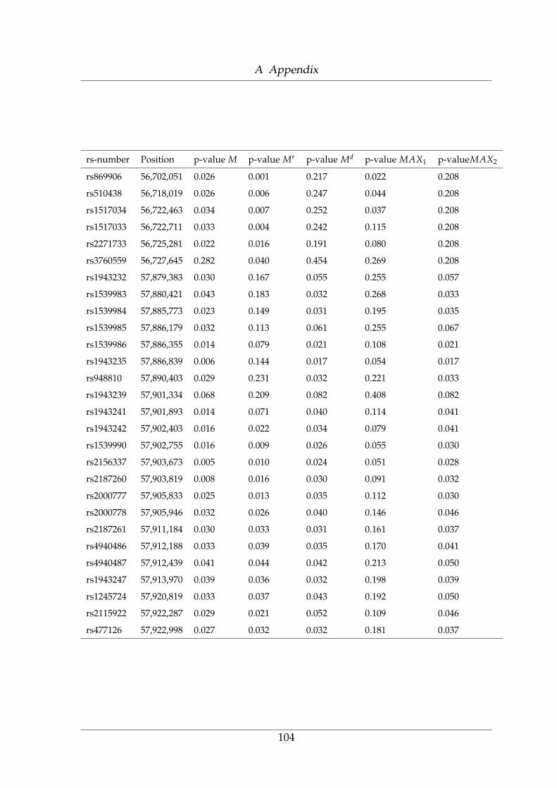
A Appendix


rs869906 56,702,051 0.026 0.001 0.217 0.022 0.208

rs510438 56,718,019 0.026 0.006 0.247 0.044 0.208

rs1517034 56,722,463 0.034 0.007 0.252 0.037 0.208

rs1517033 56,722,711 0.033 0.004 0.242 0.115 0.208

rs2271733 56,725,281 0.022 0.016 0.191 0.080 0.208

rs3760559 56,727,645 0.282 0.040 0.454 0.269 0.208

rs1943232 57,879,383 0.030 0.167 0.055 0.255 0.057

rs1539983 57,880,421 0.043 0.183 0.032 0.268 0.033

rs1539984 57,885,773 0.023 0.149 0.031 0.195 0.035

rs1539985 57,886,179 0.032 0.113 0.061 0.255 0.067

rs1539986 57,886,355 0.014 0.079 0.021 0.108 0.021

rs1943235 57,886,839 0.006 0.144 0.017 0.054 0.017

rs948810 57,890,403 0.029 0.231 0.032 0.221 0.033

rs1943239 57,901,334 0.068 0.209 0.082 0.408 0.082

rs1943241 57,901,893 0.014 0.071 0.040 0.114 0.041

rs1943242 57,902,403 0.016 0.022 0.034 0.079 0.041

rs1539990 57,902,755 0.016 0.009 0.026 0.055 0.030

rs2156337 57,903,673 0.005 0.010 0.024 0.051 0.028

rs2187260 57,903,819 0.008 0.016 0.030 0.091 0.032

rs2000777 57,905,833 0.025 0.013 0.035 0.112 0.030

rs2000778 57,905,946 0.032 0.026 0.040 0.146 0.046

rs2187261 57,911,184 0.030 0.033 0.031 0.161 0.037

rs4940486 57,912,188 0.033 0.039 0.035 0.170 0.041

rs4940487 57,912,439 0.041 0.044 0.042 0.213 0.050

rs1943247 57,913,970 0.039 0.036 0.032 0.198 0.039

rs1245724 57,920,819 0.033 0.037 0.043 0.192 0.050

rs2115922 57,922,287 0.029 0.021 0.052 0.109 0.046

rs477126 57,922,998 0.027 0.032 0.032 0.181 0.037

104

A Appendix


rs534520 57,924,186 0.030 0.030 0.027 0.167 0.035

rs1977961 57,924,643 0.024 0.020 0.028 0.126 0.035

rs1560399 57,927,016 0.023 0.029 0.029 0.128 0.043

rs2051342 57,930,468 0.018 0.023 0.013 0.096 0.022

rs1560402 57,931,505 0.008 0.015 0.018 0.063 0.020

rs580563 57,931,745 0.011 0.028 0.019 0.078 0.026

rs1579502 57,937,608 0.011 0.024 0.010 0.054 0.100

rs500817 57,939,324 0.006 0.012 0.005 0.035 0.079

rs610634 57,941,951 0.011 0.037 0.004 0.031 0.050

rs515705 57,946,659 0.038 0.046 0.017 0.114 0.199

rs546912 57,947,789 0.015 0.054 0.002 0.029 0.063

rs505289 57,949,273 0.004 0.328 0.001 0.017 0.025

rs582970 57,949,433 0.010 0.049 0.010 0.003 0.007

rs483145 57,953,275 0.001 0.076 0.001 0.004 0.012

rs949292 57,953,781 0.001 0.068 0.004 0.007 0.019

rs505487 57,954,288 0.002 0.079 0.005 0.005 0.005

rs585663 57,955,857 0.010 0.045 0.004 0.005 0.004

rs662129 57,958,259 0.010 0.036 0.006 0.004 0.006

rs585187 57,962,098 0.010 0.047 0.007 0.001 0.008

rs581526 57,962,857 0.010 0.069 0.005 0.004 0.005

rs575864 57,967,458 0.004 0.111 0.007 0.028 0.008

rs489310 57,968,905 0.010 0.134 0.008 0.015 0.008

rs590915 57,969,530 0.006 0.256 0.006 0.056 0.006

rs2003282 57,972,022 0.020 0.236 0.009 0.065 0.009

rs472418 57,972,439 0.016 0.297 0.013 0.069 0.014

rs629493 57,972,818 0.014 0.269 0.008 0.067 0.009

rs522919 57,982,374 0.068 0.292 0.046 0.270 0.052

rs514863 57,982,830 0.037 0.255 0.034 0.229 0.039

105

A Appendix


rs565368 57,983,837 0.029 0.249 0.039 0.226 0.046

rs563729 57,983,987 0.039 0.274 0.041 0.254 0.052

rs1430384 57,984,123 0.048 0.195 0.046 0.241 0.046

rs1430394 58,032,614 0.024 0.434 0.011 0.042 0.011

rs603119 58,041,625 0.015 0.450 0.010 0.048 0.011

rs4588087 58,079,680 0.005 0.410 0.007 0.038 0.007

rs2163279 58,080,585 0.006 0.420 0.011 0.029 0.011

rs1954999 58,090,607 0.034 0.501 0.009 0.067 0.009

rs2000833 58,097,914 0.031 0.484 0.014 0.056 0.014

rs1430390 58,098,321 0.037 0.495 0.011 0.052 0.011

rs4613170 58,101,493 0.031 0.501 0.009 0.054 0.009

rs1430373 58,102,862 0.024 0.508 0.008 0.065 0.008

rs2217442 58,105,690 0.041 0.494 0.015 0.037 0.015

rs1430376 58,106,598 0.032 0.490 0.013 0.057 0.013

rs1430382 58,110,412 0.025 0.481 0.007 0.041 0.006

rs1954995 58,111,342 0.035 0.489 0.009 0.057 0.009

rs1954996 58,111,459 0.023 0.495 0.012 0.037 0.012

rs1954997 58,111,571 0.024 0.489 0.012 0.065 0.012

rs721247 58,113,283 0.035 0.494 0.013 0.045 0.013

rs1079174 58,119,896 0.031 0.481 0.013 0.052 0.013

rs1079139 58,120,334 0.028 0.462 0.010 0.050 0.010

rs985044 58,122,257 0.034 0.485 0.008 0.064 0.008

rs4940954 58,127,526 0.033 0.488 0.008 0.063 0.008

rs1430369 58,129,302 0.018 0.504 0.006 0.062 0.007

rs1430371 58,130,099 0.033 0.508 0.011 0.068 0.011

rs1017797 58,130,319 0.047 0.470 0.010 0.055 0.010

rs4940957 58,131,697 0.044 0.478 0.011 0.076 0.013

rs1478526 58,134,001 0.025 0.455 0.017 0.047 0.017

106

A Appendix


rs1382392 58,135,974 0.031 0.468 0.010 0.045 0.011

rs1382394 58,136,368 0.038 0.473 0.011 0.058 0.011

rs1351154 58,139,501 0.032 0.473 0.011 0.053 0.011

rs4940960 58,143,841 0.022 0.501 0.008 0.056 0.008

rs4940494 58,145,032 0.014 0.490 0.009 0.030 0.009

rs1455498 58,150,654 0.035 0.476 0.006 0.032 0.006

rs1455499 58,150,869 0.032 0.491 0.004 0.049 0.004

rs2332069 58,159,567 0.029 0.493 0.010 0.033 0.010

rs2061793 58,160,649 0.043 0.478 0.006 0.028 0.006

rs1455526 58,161,174 0.016 0.484 0.007 0.031 0.007

rs1455525 58,162,058 0.021 0.441 0.006 0.031 0.006

rs931078 58,167,676 0.012 0.467 0.004 0.028 0.004

rs899262 58,168,645 0.020 0.470 0.009 0.046 0.009

rs899261 58,168,784 0.015 0.474 0.006 0.059 0.006

rs4940966 58,169,787 0.028 0.468 0.008 0.036 0.008

rs4940498 58,177,215 0.022 0.488 0.011 0.034 0.012

rs1118433 58,179,494 0.028 0.460 0.011 0.048 0.012

rs987372 58,181,285 0.021 0.497 0.010 0.046 0.010

rs1471040 58,183,449 0.013 0.471 0.005 0.028 0.005

rs1017796 58,184,444 0.028 0.486 0.006 0.026 0.006

rs1455510 58,186,404 0.014 0.479 0.004 0.036 0.005

rs1455506 58,197,094 0.028 0.491 0.004 0.042 0.004

rs1564223 58,197,868 0.026 0.456 0.009 0.034 0.009

rs1455504 58,202,391 0.023 0.479 0.007 0.046 0.008

rs1455500 58,203,710 0.017 0.451 0.005 0.027 0.005

rs2332026 58,206,156 0.020 0.478 0.011 0.048 0.011

rs967809 58,220,698 0.035 0.494 0.016 0.075 0.016

rs1455515 58,221,725 0.025 0.492 0.009 0.082 0.009

107

A Appendix


rs1947779 58,222,879 0.019 0.488 0.008 0.057 0.008

rs1072733 58,225,463 0.016 0.486 0.007 0.039 0.007

rs1378483 58,226,033 0.029 0.454 0.010 0.041 0.010

rs2219193 58,240,339 0.028 0.478 0.014 0.063 0.014

rs4940973 58,243,941 0.024 0.482 0.009 0.066 0.009

rs2332023 58,253,461 0.021 0.500 0.009 0.049 0.009

rs4940974 58,258,384 0.039 0.480 0.022 0.085 0.022

rs3898175 58,268,358 0.051 0.467 0.012 0.074 0.012

rs4452046 58,269,313 0.033 0.469 0.013 0.081 0.013

rs1350044 58,274,464 0.027 0.470 0.010 0.076 0.010

rs1455523 58,276,783 0.041 0.472 0.021 0.080 0.021

rs1982636 58,277,099 0.033 0.478 0.017 0.077 0.017

rs1993888 58,277,751 0.013 0.463 0.012 0.047 0.012

rs1993890 58,278,095 0.016 0.478 0.013 0.049 0.013

rs1378489 58,279,195 0.029 0.493 0.009 0.065 0.009

rs1993355 58,282,103 0.040 0.479 0.023 0.120 0.022

rs1455519 58,290,272 0.068 0.495 0.025 0.153 0.026

rs1455520 58,290,674 0.054 0.481 0.033 0.144 0.035

rs4245285 58,302,709 0.066 0.521 0.033 0.146 0.033

rs4940508 58,356,160 0.059 0.368 0.029 0.163 0.028

rs4940984 58,357,110 0.058 0.379 0.047 0.124 0.048

rs1497981 58,369,964 0.110 0.404 0.043 0.188 0.045

rs1497965 58,374,101 0.117 0.362 0.048 0.217 0.050

108

Acknowledgments

First of all, I am very grateful for the advice of my advisor, Prof. Dr. Andreas

Ziegler, during my doctoral studies. Particularly, I wish to express my thanks to him

for his encouragement and introducing me to this exciting research field. I always

feel lucky and am proud of working with him. I also appreciate his assistance in

writing.

I am greatly indebted to Priv.-Doz. Dr. Inke R. Konig for her never ending support

and their valuable suggestions of my work. I also would like to thank Dr. Michael

Brendel for providing many useful comments and suggestions, and Jordis Stolp-

mann for her help with the german language. Last but the most important I want to

give many thanks to my colleagues in our laboratory for the friendly atmosphere in

our group and their help with both technical and personal difficulties. In particular,

I would like to thank Mrs. Gabriele Schatton for her cooperation and assistance.

Support for generation of the simulated data was provided from NIH grants 5RO1-

HL049609-14, 1R01-AG021917-01A1, the University of Minnesota, and the Minnesota

Supercomputing Institute. The GAW is supported by the Grant R01 GM031575.

I am grateful to Peter K. Gregersen and the investigators in the North American

Rheumatoid Arthritis Consortium (NARAC) for allowing us to use their genotyping

109

A Appendix

data for this study. The original data collection was supported by a grant from the

National Institutes of Health, RO1 AR44422 and NO1-AR-2-2263.

I owe my deepest gratitude to my family, my wife and special girls, for their endless

love and encouragement during my study.

110

Curriculum vitae

Personal data Adel Ali Ewhida

Al-Fateh University, Faculty of Science, Department of Statistics

P.O. Box 13219, Tripoli Libya

Tel.: (+218) 92 280 7661

E-Mail: [email protected]

Birth: 12.02.1968 in Tripoli Libya

married

School education

1974 – 1980 Primary school in Libya

1980 – 1986 Secondary school in Libya

July 1986 High school in Libya

111

A Appendix

University studies

1986 – 1990 Bachelor of Science (B.Sc.) in Statistics from Nasser University

in Libya

1996 – 2000 Master of Science (M.Sc.) in Statistics from Saskatchewan Uni-

versity in Canada. Thesis Topic: Long Tail Distributions (Ap-

proximating the long tail distributions by finite mixtures of ex-

ponential distributions)

Professional development

1993 – 1995 I worked as teaching assistant at the Department of Statistics at

Al Fateh University in Libya

1993 – 1996 I taught computer Applications in Statistics at High Institute of

computer Technology in Libya

1997 – 1999 I worked as Lab assistant and marker in the Department of Math-

ematics and Statistics at the University of Saskatchewan in Canada

1999 – 2003 I worked as lecturer assistant in the Department of Statistics at

Al Fateh University in Libya

May 28, 2009

112

Publikation and Abstracts

de Andrade, M., M and Allen, A. S., Brinza, D. , Cheng, R.,Da, Y.,de Vries, A.

R.,Ewhida, A.,Feng, Z.,Jung, H.,Hsieh, H. J.& others (2007) Summary of contri-

butions to GAW15 Group 13: candidate gene association studies. Genet Epidemiol,

31 Suppl 1: S110-S117.

Ziegler, A., Ewhida A., Brendel M. & Kleensang A. (2008) More Powerful Haplotype

Sharing by Accounting for the Mode of Inheritance. Genet Epidemiol, Wiley-Liss,

Inc. (Epub).

113

Haplotype Sharing by Accounting for the Mode of Inheritance · beneﬁts in some cases, for example...

Documents

Transcript of Haplotype Sharing by Accounting for the Mode of Inheritance · beneﬁts in some cases, for example...