Hans Gilgen Univariate Time Series in Geosciences Theory and Examples

Hans Gilgen

Univariate Time Series in Geosciences Theory and Examples

With 220 Figures

AUTHOR: Dr. Hans GilgenInstitute for Atmospheric and Climate Science Swiss Federal Institute of Technology (ETH) ZurichUniversitätsstr. 16 8092 ZurichSwitzerland E-MAIL: HANS.GILGEN@ENV.ETHZ.CH ISBN 10 3-540-23810-7 Springer Berlin Heidelberg New York ISBN 13 978-3-540-23810-2 Springer Berlin Heidelberg New York Library of Congress Control Number: 2005933719 This work is subject to copyright. All rights are reserved, whether the whole or part of the material is concerned, specifically the rights of translation, reprinting, reuse of illustrations, recitation, broad-casting, reproduction on microfilm or in any other way, and storage in data banks. Duplication of this publication or parts thereof is permitted only under the provisions of the German Copyright Law of September 9, 1965, in its current version, and permission for use must always be obtained from Springer-Verlag. Violations are liable to prosecution under the German Copyright Law. Springer is a part of Springer Science+Business Media springeronline.com © Springer-Verlag Berlin Heidelberg 2006 Printed in The Netherlands The use of general descriptive names, registered names, trademarks, etc. in this publication does not imply, even in the absence of a specific statement, that such names are exempt from the relevant pro-tective laws and regulations and therefore free for general use. Cover design: E. Kirchner, Heidelberg Production: A. Oelschläger Typesetting: Camera-ready by the Author Printed on acid-free paper 30/2132/AO 543210

in memory of JoJo and MaiMaito Lusai

Preface

La theorie des probabilites n’est au fond que le bon sens reduit au calcul.Probability theory is, basically, nothing but common sense reduced to

calculation.Laplace, Essai Philosophique sur les Probabilites, 1814.

In Geosciences, variables depending on space and time have been mea-sured for decades or even centuries. Temperature for example has been ob-served worldwide since approximately 1860 under international standards(those of the World Meteorological Organisation (WMO)). A much shorterinstrumental (i.e., measured with instruments) record of the global back-ground concentration of atmospheric carbon dioxide is available for Hawaii(Mauna Loa Observatory) only dating back to 1958, owing to difficulties in-herent in the routine measurement of atmospheric carbon dioxide. Furtherexamples of long-term records are those obtained from measurements of riverdischarge.

In contrast to standardised routine measurements, variables are also mea-sured in periods and regions confined in time and space. For example, (i)ground water permeability in a gravel deposit can be approximated from grainsize distributions of a few probes taken (owing to limited financial resourcesfor exploring the aquifer), (ii) solar radiation at the top of the atmospherehas been measured by NASA in the Earth Radiation Budget Experimentfor the period from November 1984 through to February 1990 using instru-ments mounted on satellites (since the lifetime of radiation instruments inspace is limited), (iii) three-dimensional velocities of a turbulent flow in theatmospheric boundary layer can be measured during an experiment (seeingthat a measurement campaign is too costly to maintain for decades), and lastbut not least (iv), measurements have been performed under often extremelyadverse conditions on expeditions.

Many variables analysed in Geosciences depend not only on space andtime but also on chance. Depending on chance means that (i) all recordsobserved are reconcilable with a probabilistic model and (ii) no determinis-tic model is available that better fits the observations or is better suited forpractical applications, e.g., allows for better predictions. Deterministic mod-

VIII Preface

els have become more and more sophisticated with the increasing amountof computing power available, an example being the generations of climatemodels developed in the last two decades. Nevertheless, tests, diagnosticsand predictions based on probabilistic models are applied with increasingfrequency in Geosciences. For example, using probabilistic models (i) theNorth Atlantic Oscillation (NAO) index has been found to be stationary inits mean, i.e., its mean neither increases nor decreases systematically withinthe observational period, (ii) decadal changes in solar radiation incident atthe Earth’s surface have been estimated for most regions with long-term solarradiation records, (iii) Geostatistical methods for the optimal interpolationof spatial random functions, developed and applied by mining engineers forexploring and exploiting ore deposits, are now used with increasing frequencyin many disciplines, e.g., in water resources management, forestry, agricultureor meteorology, and (iv) turbulent flows in the atmospheric boundary layerare described statistically in most cases.

If a variable depending on space and/or time is assumed to be in agree-ment with a probabilistic model then it is treated as a stochastic process orrandom function. Under this assumption, observations stem from a realisa-tion of a random function and are not independent, precisely because thevariable being observed depends on space and time. Consequently, standardstatistical methods can only be applied under precautions since they assumeindependent and identically distributed observations, the assumptions madein an introduction to Statistics.

Often, geophysical observations of at least one variable are performed ata fixed location (a site or station) using a constant sampling interval, andtime is recorded together with the measured values. A record thus obtainedis a time series. A univariate time series is a record of observations of onlyone variable: a multivariate one of simultaneous observations of at least twovariables. Univariate time series are analysed in this book under the assump-tion that they stem from discrete-time stochastic processes. The restrictionto univariate series prevents this book from becoming too long.

In contrast to the other examples given, the Mauna Loa atmosphericcarbon dioxide record grows exponentially, a property often found in socio-economic data. For example, the power consumed in the city of Zurich growsexponentially, as demonstrated in this book.

Subsequent to introducing time series and stochastic processes in Chaps. 1and 2, probabilistic models for time series are estimated in the time domain.An estimation of such models is feasible on condition that the time series ob-served are reconcilable with suitable assumptions. Among these, stationarityplays a prominent role. In Chap. 3, a non-constant expectation function of thestochastic process under analysis is captured by means of estimating a linearmodel using regression methods. Chap. 4 introduces the estimation of mod-els for the covariance function of a spatial random function using techniquesdeveloped in Geostatistics. These models are thereafter used to compute op-

Preface IX

timal interpolators. Optimal interpolators are a version of optimal predictors,both being estimators in the statistical sense. In Chap. 5, optimal predictorsfor a time series are obtained by applying models for the underlying stochas-tic process itself. These models are called linear processes, ARMA modelsor Box-Jenkins-models. Chap. 3 should be read prior to tackling Chap. 4 orChap. 5; it is, however, not necessary to read Chap. 4 prior to accepting thechallenge of Chap. 5.

Chaps. 6, 7, 8, 9 and 10 give an introduction to time series analysis in thefrequency domain. In Chap. 6, Fourier analysis of deterministic functions iscomprehensively (including discussions of aliasing, leakage and the width offunctions in both domains, time and frequency) dealt with in order to build asolid framework supporting the application of Fourier methods to time series,which is legitimised by the Fourier representation of stationary stochasticprocesses introduced in Chap. 7. Under these preconditions, estimators for thespectrum of a stationary stochastic process under analysis can be calculatedfrom a time series observed.

In Chap. 8, the periodogram is introduced. The periodogram has anasymptotic distribution that can be derived for most discrete-time stationarystochastic processes. Unfortunately, a periodogram calculated from a realisa-tion of a process having a spectrum with a large dynamic range is severelybiased and thus the periodogram is generally not a spectral estimator. Spec-tral estimators are calculated from tapered observations, i.e., observationsmodified using a data window, a technique that efficiently reduces the biasdue to leakage. In Chap. 9, an estimator calculated from tapered observationsis convolved with a smoothing kernel to obtain an estimator for a continu-ous spectrum, and Chap. 10 contains a short introduction to estimators fordiscrete spectra.

This book is intended to be an introduction to the analysis of time seriesfor students of Geosciences, who are assumed to have a mathematical back-ground of at least two semesters calculus and one semester probability theoryand statistics.

I composed this book using LATEX together with macros made availableby Springer-Verlag and also prepared all figures, except for Fig. 3.10, whichis credited to S. Bischof.

This book appears for the twentieth anniversary of preliminary and in-complete versions of Chaps. 2, 3, 4, 5, 6, 9 and 10 which I used in coursesgiven to students of atmospheric and earth sciences at the Swiss Federal In-stitute of Technology (ETH) and the University, both in Zurich. The studentslearnt to estimate models for example time series (of these, the Basel tem-perature series has “survived” as can be seen in Table 1.1) and I learnt thatclear definitions are important, obviously not a novel concept. My coursesevolved together with the statistical software being available and also perti-nent to teaching. The major evolutionary step was the changeover to Splusin the early 1990s. Splus proved to be the first statistical software that could

X Preface

be successfully applied by the students subsequent to a short introduction.Three years ago, a small number of example programs and exercises weremodified so that R could be used. The reasons for these last changes weretwofold: (i) I believed (and still believe) that R will develop more dynamicallythan Splus and (ii) R is available under Gnu conditions.

My time series courses improved with the help of H. Kunsch of the Statis-tics Seminar at ETH. He gave a large number of valuable suggestions andhis comments on earlier versions (in German) motivated me to write in sucha way that the mathematics is correct and the text remains readable fornon-mathematicians. The English version was corrected by D. Scherrer whocarefully read the manuscript and patiently transformed German-like con-structions into English. Without the help of both, H. Kunsch and D. Scherrer,this book could not have been written.

C. Hohenegger’s critical comments helped to fine-tune the definitions andderivations given in this book.

I am indebted to (i) H. Jensen for entrusting me with preliminary versionsof Sects. 4.3.2, 4.5.2, 4.5.3 and 4.6.3, (ii) K. Hutter for encouraging me towrite this book and (iii) Atsumu Ohmura for both, his confidence in thisproject and funding at critical times that helped to finish this book.

I thank M. Andretta, M. Bannert, R. Barry, H. Blatter, C. Breitinger,S. Bronnimann, N. Bukowieki, P. Calanca, H. Fischer, C. Frei, M. Giansir-acusa, D. Grebner, J. Gurtz, A. Hanger, H. Jensen, M. Machler, G. Muller,Andree and Atsumu Ohmura, A. Roesch, M. Rotach, M. Roth, W. Sawyer,P. Stamp, F. Stauffer, H. von Storch, M. Wild and M. Zappa for supplyingdata and/or commenting on (parts of) the manuscript. I also thank all stu-dents whose comments helped to improve the manuscript and the exercises.Any errors remaining are my responsibility and any comments are welcome.

Zurich, July, 2005 Hans GilgenInstitute for Atmospheric and Climate Science

Swiss Federal Institute of Technology (ETH) ZurichUniversitatsstrasse 16

CH-8092 Zurichgilgen@env.ethz.ch

Contents

1 Introduction . . . . . . . . . . . . . . . . . . . . . . . . . . . . . . . . . . . . . . . . . . . . . . 11.1 Data in Geosciences: for Example, Surface Solar Radiation

Records . . . . . . . . . . . . . . . . . . . . . . . . . . . . . . . . . . . . . . . . . . . . . . . 11.2 R. . . . . . . . . . . . . . . . . . . . . . . . . . . . . . . . . . . . . . . . . . . . . . . . . . . . . 81.3 Independent Identically Distributed (Iid.) Random Variables . 10

1.3.1 Univariate Analysis of the Pyranometer Data . . . . . . . . 101.3.2 Unbiased and Consistent Estimators, Central Limit

Theorem . . . . . . . . . . . . . . . . . . . . . . . . . . . . . . . . . . . . . . . . 131.3.3 Bivariate Analysis of the Pyranometer Data . . . . . . . . . 171.3.4 Are the Pyranometer Daily Values Iid.? . . . . . . . . . . . . . 22

1.4 Time Series . . . . . . . . . . . . . . . . . . . . . . . . . . . . . . . . . . . . . . . . . . . . 231.4.1 Time Series Plots . . . . . . . . . . . . . . . . . . . . . . . . . . . . . . . . . 231.4.2 A Model for the Error of the Pyranometer

Measurements . . . . . . . . . . . . . . . . . . . . . . . . . . . . . . . . . . . 301.5 Supplements . . . . . . . . . . . . . . . . . . . . . . . . . . . . . . . . . . . . . . . . . . . 31

1.5.1 Formulas for Calculating the Moments of RandomVariables . . . . . . . . . . . . . . . . . . . . . . . . . . . . . . . . . . . . . . . . 31

1.5.2 Chebyshev Inequality . . . . . . . . . . . . . . . . . . . . . . . . . . . . . 321.5.3 Independent and Normally Distributed Random

Variables . . . . . . . . . . . . . . . . . . . . . . . . . . . . . . . . . . . . . . . . 321.5.4 Bivariate (two-dimensional) Normal Density . . . . . . . . . 341.5.5 Multivariate Normal Distribution . . . . . . . . . . . . . . . . . . . 35

1.6 Problems . . . . . . . . . . . . . . . . . . . . . . . . . . . . . . . . . . . . . . . . . . . . . . 36

2 Stationary Stochastic Processes . . . . . . . . . . . . . . . . . . . . . . . . . . . 392.1 Empirical Moments of a Wind Speed Time Series . . . . . . . . . . . 392.2 Stationary Stochastic Processes . . . . . . . . . . . . . . . . . . . . . . . . . . 44

2.2.1 Stochastic Processes . . . . . . . . . . . . . . . . . . . . . . . . . . . . . . 442.2.2 1st and 2nd Moment Functions . . . . . . . . . . . . . . . . . . . . . 502.2.3 Stationarity Assumptions . . . . . . . . . . . . . . . . . . . . . . . . . . 52

2.3 Discrete-time Stochastic Processes . . . . . . . . . . . . . . . . . . . . . . . . 562.3.1 White Noise Process . . . . . . . . . . . . . . . . . . . . . . . . . . . . . . 562.3.2 First Order Autoregressive (AR[1]) Process . . . . . . . . . . 602.3.3 Random Walk . . . . . . . . . . . . . . . . . . . . . . . . . . . . . . . . . . . 642.3.4 First Order Moving Average Process . . . . . . . . . . . . . . . . 66

XII Contents

2.3.5 Linear Process . . . . . . . . . . . . . . . . . . . . . . . . . . . . . . . . . . . 702.4 Convolution I . . . . . . . . . . . . . . . . . . . . . . . . . . . . . . . . . . . . . . . . . . 74

2.4.1 Linear and Time-invariant Transformations . . . . . . . . . . 742.4.2 Existence and Calculation of Convolution Sums . . . . . . 782.4.3 Inverse Sequences . . . . . . . . . . . . . . . . . . . . . . . . . . . . . . . . 822.4.4 Examples: AR[1] and AR[2] Models . . . . . . . . . . . . . . . . . 84

2.5 When Is a Time Series Stationary? . . . . . . . . . . . . . . . . . . . . . . . 882.5.1 Diagnostics for the Stationarity of a Time Series . . . . . 882.5.2 Locally Stationary Time Series . . . . . . . . . . . . . . . . . . . . . 92

2.6 Estimators for the Moment Functions of a StationaryStochastic Process . . . . . . . . . . . . . . . . . . . . . . . . . . . . . . . . . . . . . . 972.6.1 Properties of the Empirical Moment Functions of a

Stationary Time Series . . . . . . . . . . . . . . . . . . . . . . . . . . . . 972.6.2 Ergodic Theorems: a Cautionary Remark . . . . . . . . . . . . 101

2.7 Optimal Linear Predictions . . . . . . . . . . . . . . . . . . . . . . . . . . . . . . 1022.8 Supplements . . . . . . . . . . . . . . . . . . . . . . . . . . . . . . . . . . . . . . . . . . . 104

2.8.1 First and/or second Moment Functions of someProcesses . . . . . . . . . . . . . . . . . . . . . . . . . . . . . . . . . . . . . . . . 104

2.8.2 Moments of the Mean of a Stationary Time Series . . . . 1062.8.3 Properties of the Optimal Linear Prediction . . . . . . . . . 1082.8.4 The Conditional Expectation as Optimal Prediction . . 111

2.9 Problems . . . . . . . . . . . . . . . . . . . . . . . . . . . . . . . . . . . . . . . . . . . . . . 113

3 Linear Models for the Expectation Function . . . . . . . . . . . . . . 1213.1 Simple Linear Regression . . . . . . . . . . . . . . . . . . . . . . . . . . . . . . . . 122

3.1.1 An Introductory Example . . . . . . . . . . . . . . . . . . . . . . . . . 1223.1.2 Simple Linear Regression . . . . . . . . . . . . . . . . . . . . . . . . . . 125

3.2 Multiple Regression . . . . . . . . . . . . . . . . . . . . . . . . . . . . . . . . . . . . . 1303.2.1 A Linear Model for the Expectation Function . . . . . . . . 1303.2.2 Least Squares . . . . . . . . . . . . . . . . . . . . . . . . . . . . . . . . . . . . 1323.2.3 Independent Observations with Constant Variance . . . . 1333.2.4 Generalised least squares . . . . . . . . . . . . . . . . . . . . . . . . . . 1333.2.5 Normally distributed residuals . . . . . . . . . . . . . . . . . . . . . 136

3.3 Diagnostics for Linear Models . . . . . . . . . . . . . . . . . . . . . . . . . . . . 1363.3.1 Plots . . . . . . . . . . . . . . . . . . . . . . . . . . . . . . . . . . . . . . . . . . . 1363.3.2 Model Selection . . . . . . . . . . . . . . . . . . . . . . . . . . . . . . . . . . 142

3.4 Seasonal and Component Models . . . . . . . . . . . . . . . . . . . . . . . . . 1453.4.1 Seasonal Models . . . . . . . . . . . . . . . . . . . . . . . . . . . . . . . . . . 1453.4.2 Component Models . . . . . . . . . . . . . . . . . . . . . . . . . . . . . . . 148

3.5 Trends and Station Effects of Shortwave Incoming Radiation . 1513.6 Trend Surfaces for the Tree-line in the Valais Alps . . . . . . . . . . 1613.7 Problems . . . . . . . . . . . . . . . . . . . . . . . . . . . . . . . . . . . . . . . . . . . . . . 167

Contents XIII

4 Interpolation . . . . . . . . . . . . . . . . . . . . . . . . . . . . . . . . . . . . . . . . . . . . . 1714.1 Deterministic Interpolation . . . . . . . . . . . . . . . . . . . . . . . . . . . . . . 173

4.1.1 Distance Weighted Interpolation . . . . . . . . . . . . . . . . . . . 1734.1.2 Tessellation of the Area under Study . . . . . . . . . . . . . . . . 1784.1.3 Discussion . . . . . . . . . . . . . . . . . . . . . . . . . . . . . . . . . . . . . . . 180

4.2 The Spatial Random Function and its Variogram . . . . . . . . . . . 1814.3 Estimating the Variogram . . . . . . . . . . . . . . . . . . . . . . . . . . . . . . . 185

4.3.1 Empirical Variograms I: the Isotropic Case . . . . . . . . . . 1864.3.2 Variogram Models . . . . . . . . . . . . . . . . . . . . . . . . . . . . . . . . 1934.3.3 Empirical Variograms II: the Anisotropic Case . . . . . . . 1964.3.4 Empirical Variograms III: the Case with Non-constant

Drift . . . . . . . . . . . . . . . . . . . . . . . . . . . . . . . . . . . . . . . . . . . . 2004.4 Optimal Linear Predictors for Spatial Random Functions . . . . 2064.5 Optimal Interpolation of Spatial Random Functions . . . . . . . . 209

4.5.1 The Stationary Case: Simple Kriging . . . . . . . . . . . . . . . 2094.5.2 The Intrinsic Case: Ordinary Kriging . . . . . . . . . . . . . . . 2154.5.3 The Case with a Non-constant Drift: Universal Kriging 2164.5.4 Summary. . . . . . . . . . . . . . . . . . . . . . . . . . . . . . . . . . . . . . . . 222

4.6 Supplements . . . . . . . . . . . . . . . . . . . . . . . . . . . . . . . . . . . . . . . . . . . 2254.6.1 Isotropic Empirical Variograms . . . . . . . . . . . . . . . . . . . . . 2254.6.2 Support . . . . . . . . . . . . . . . . . . . . . . . . . . . . . . . . . . . . . . . . . 2274.6.3 Measurement Errors . . . . . . . . . . . . . . . . . . . . . . . . . . . . . . 2294.6.4 Local Interpolation . . . . . . . . . . . . . . . . . . . . . . . . . . . . . . . 2364.6.5 Spatial Averages . . . . . . . . . . . . . . . . . . . . . . . . . . . . . . . . . 2394.6.6 Optimal Interpolation: Summary . . . . . . . . . . . . . . . . . . . 243

4.7 Problems . . . . . . . . . . . . . . . . . . . . . . . . . . . . . . . . . . . . . . . . . . . . . . 244

5 Linear Processes . . . . . . . . . . . . . . . . . . . . . . . . . . . . . . . . . . . . . . . . . . 2495.1 AR[p] Models . . . . . . . . . . . . . . . . . . . . . . . . . . . . . . . . . . . . . . . . . . 250

5.1.1 The Yule-Walker-Equations of an AR[p] Model . . . . . . . 2515.1.2 Levinson-Durbin Recursion, Partial Correlation

Function . . . . . . . . . . . . . . . . . . . . . . . . . . . . . . . . . . . . . . . . 2555.1.3 Examples . . . . . . . . . . . . . . . . . . . . . . . . . . . . . . . . . . . . . . . 257

5.2 Estimating an AR[p] Model . . . . . . . . . . . . . . . . . . . . . . . . . . . . . . 2625.2.1 Burg’s Algorithm . . . . . . . . . . . . . . . . . . . . . . . . . . . . . . . . . 2625.2.2 Regression Estimates . . . . . . . . . . . . . . . . . . . . . . . . . . . . . 2645.2.3 Maximum Likelihood Estimates . . . . . . . . . . . . . . . . . . . . 2665.2.4 Summary of Sects. 5.1 and 5.2 . . . . . . . . . . . . . . . . . . . . . 269

5.3 MA[q] , ARMA[p, q] and ARIMA[p, d, q] Models . . . . . . . . . . . . 2715.3.1 MA[q] Model . . . . . . . . . . . . . . . . . . . . . . . . . . . . . . . . . . . . 2715.3.2 ARMA[p, q] Model . . . . . . . . . . . . . . . . . . . . . . . . . . . . . . . . 2755.3.3 ARIMA[p, d, q] Model . . . . . . . . . . . . . . . . . . . . . . . . . . . . . 2795.3.4 Estimators for an ARMA[p, q] Model . . . . . . . . . . . . . . . . 280

5.4 Fitting an ARIMA[p, d, q] Model . . . . . . . . . . . . . . . . . . . . . . . . . 282

XIV Contents

5.4.1 Removing Trends or other Fluctuations from a TimeSeries . . . . . . . . . . . . . . . . . . . . . . . . . . . . . . . . . . . . . . . . . . . 282

5.4.2 Identification . . . . . . . . . . . . . . . . . . . . . . . . . . . . . . . . . . . . 2895.4.3 Estimation . . . . . . . . . . . . . . . . . . . . . . . . . . . . . . . . . . . . . . 2955.4.4 Diagnostics . . . . . . . . . . . . . . . . . . . . . . . . . . . . . . . . . . . . . . 2975.4.5 Selection and Summary . . . . . . . . . . . . . . . . . . . . . . . . . . . 304

5.5 Predictions . . . . . . . . . . . . . . . . . . . . . . . . . . . . . . . . . . . . . . . . . . . . 3065.5.1 Predictions Using a Theoretical ARMA[p, q] Model . . . 3065.5.2 Predictions Using an Estimated ARMA[p, q] Model . . . 3115.5.3 Summary. . . . . . . . . . . . . . . . . . . . . . . . . . . . . . . . . . . . . . . . 313

5.6 Supplements . . . . . . . . . . . . . . . . . . . . . . . . . . . . . . . . . . . . . . . . . . . 3145.6.1 Levinson-Durbin Recursion . . . . . . . . . . . . . . . . . . . . . . . . 3145.6.2 Partial Correlation Function . . . . . . . . . . . . . . . . . . . . . . . 3165.6.3 Predictions Derived from the AR[∞] and MA[∞]

representations of an ARMA[p, q] Model . . . . . . . . . . . . . 3185.6.4 Predictions Derived from the Difference Equation of

an ARMA[p, q] Model . . . . . . . . . . . . . . . . . . . . . . . . . . . . . 3205.7 Problems . . . . . . . . . . . . . . . . . . . . . . . . . . . . . . . . . . . . . . . . . . . . . . 322

6 Fourier Transforms of Deterministic Functions . . . . . . . . . . . . 3296.1 Adding Trigonometric Functions. . . . . . . . . . . . . . . . . . . . . . . . . . 330

6.1.1 Representation of a Sequence using TrigonometricFunctions . . . . . . . . . . . . . . . . . . . . . . . . . . . . . . . . . . . . . . . 330

6.1.2 Fouriertransforms: a Preview to Chap. 6 . . . . . . . . . . . . 3376.1.3 Spectra of Time Series: a Preview to Chaps. 7, 9 and 10338

6.2 Linear Vector Spaces . . . . . . . . . . . . . . . . . . . . . . . . . . . . . . . . . . . . 3406.2.1 Linear Vector Spaces . . . . . . . . . . . . . . . . . . . . . . . . . . . . . . 3406.2.2 Orthogonal Functions . . . . . . . . . . . . . . . . . . . . . . . . . . . . . 3436.2.3 Orthogonal Trigonometric Functions . . . . . . . . . . . . . . . . 345

6.3 Fourier Transforms . . . . . . . . . . . . . . . . . . . . . . . . . . . . . . . . . . . . . 3476.3.1 Case 1: Discrete Fourier Transform . . . . . . . . . . . . . . . . . 3476.3.2 Case 2: Fourier Series . . . . . . . . . . . . . . . . . . . . . . . . . . . . . 3536.3.3 Case 3: Fourier Integrals . . . . . . . . . . . . . . . . . . . . . . . . . . 3576.3.4 Case 4: Fourier Series with t and s Reversed . . . . . . . . . 3636.3.5 Delta Function . . . . . . . . . . . . . . . . . . . . . . . . . . . . . . . . . . . 367

6.4 Spectra . . . . . . . . . . . . . . . . . . . . . . . . . . . . . . . . . . . . . . . . . . . . . . . 3726.5 Aliasing and Leakage . . . . . . . . . . . . . . . . . . . . . . . . . . . . . . . . . . . 374

6.5.1 Measuring a Function f(t) with Real Argument t . . . . . 3756.5.2 Aliasing . . . . . . . . . . . . . . . . . . . . . . . . . . . . . . . . . . . . . . . . . 3806.5.3 Leakage . . . . . . . . . . . . . . . . . . . . . . . . . . . . . . . . . . . . . . . . . 383

6.6 Width of Functions in a Fourier Transform Pair . . . . . . . . . . . . 3896.6.1 Dynamic Range and Width at Half Height . . . . . . . . . . . 3906.6.2 Equivalent Width and σ-Width . . . . . . . . . . . . . . . . . . . . 3926.6.3 Autocorrelation Width and Uncertainty Relationship . 3946.6.4 Time-limited and Band-limited Sequences . . . . . . . . . . . 397

Contents XV

6.7 Using a Data Taper to Reduce Leakage . . . . . . . . . . . . . . . . . . . . 3996.7.1 Data Taper . . . . . . . . . . . . . . . . . . . . . . . . . . . . . . . . . . . . . . 4006.7.2 Aliasing and Leakage Circumvented . . . . . . . . . . . . . . . . . 404

6.8 Convolution II . . . . . . . . . . . . . . . . . . . . . . . . . . . . . . . . . . . . . . . . . 4086.8.1 Linear and Time-invariant (LTI) Systems . . . . . . . . . . . . 4096.8.2 First Order Differences and Moving Average . . . . . . . . . 4126.8.3 Low-pass, High-pass and Band-pass Filters . . . . . . . . . . 416

6.9 Supplements . . . . . . . . . . . . . . . . . . . . . . . . . . . . . . . . . . . . . . . . . . . 4186.9.1 Orthogonal Trigonometric Functions . . . . . . . . . . . . . . . . 4186.9.2 Discrete Fourier Transform . . . . . . . . . . . . . . . . . . . . . . . . 4206.9.3 Sums of Trigonometric Functions . . . . . . . . . . . . . . . . . . . 4206.9.4 Properties of Fourier Transform Pairs . . . . . . . . . . . . . . . 4216.9.5 Bessel’s Inequality and Parseval’s Identity . . . . . . . . . . . 4246.9.6 Properties of the Autocorrelation . . . . . . . . . . . . . . . . . . . 4256.9.7 Demonstration of the Convolution Theorem . . . . . . . . . 4286.9.8 Autocorrelation and Discrete Fourier Transform in R . 429

6.10 Problems . . . . . . . . . . . . . . . . . . . . . . . . . . . . . . . . . . . . . . . . . . . . . . 433

7 Fourier Representation of a Stationary Stochastic Process 4417.1 Independent and Poisson-distributed Events . . . . . . . . . . . . . . . 442

7.1.1 Poisson Process . . . . . . . . . . . . . . . . . . . . . . . . . . . . . . . . . . 4427.1.2 Exponential Waiting Times . . . . . . . . . . . . . . . . . . . . . . . . 4447.1.3 On-road Measurements of Aerosols . . . . . . . . . . . . . . . . . 447

7.2 Continuous-time Stochastic Processes . . . . . . . . . . . . . . . . . . . . . 4517.2.1 Random Variables in L2(Ω,F ) . . . . . . . . . . . . . . . . . . . . . 4517.2.2 Derivatives and Integrals of Random Functions . . . . . . . 4527.2.3 Examples . . . . . . . . . . . . . . . . . . . . . . . . . . . . . . . . . . . . . . . 456

7.3 Fourier Representation of a Stationary Stochastic Process . . . 4607.3.1 The Harmonic Process and its Fourier Representation . 4607.3.2 Fourier Representation of a Stationary Stochastic

Process . . . . . . . . . . . . . . . . . . . . . . . . . . . . . . . . . . . . . . . . . 4677.3.3 Covariance Function and Spectrum . . . . . . . . . . . . . . . . . 4697.3.4 Types of Spectra . . . . . . . . . . . . . . . . . . . . . . . . . . . . . . . . . 4727.3.5 Bandwidth of a Spectrum . . . . . . . . . . . . . . . . . . . . . . . . . 475

7.4 Spectra of Linear Processes . . . . . . . . . . . . . . . . . . . . . . . . . . . . . . 4777.4.1 Stochastic Filters . . . . . . . . . . . . . . . . . . . . . . . . . . . . . . . . . 4777.4.2 Examples . . . . . . . . . . . . . . . . . . . . . . . . . . . . . . . . . . . . . . . 480

7.5 Supplements . . . . . . . . . . . . . . . . . . . . . . . . . . . . . . . . . . . . . . . . . . . 4857.5.1 Gamma Distribution . . . . . . . . . . . . . . . . . . . . . . . . . . . . . . 4857.5.2 Integrating with Respect to an Orthogonal Increment

Process . . . . . . . . . . . . . . . . . . . . . . . . . . . . . . . . . . . . . . . . . 4867.5.3 Moments of the Harmonic Process . . . . . . . . . . . . . . . . . . 4897.5.4 Spectrum of a Discrete-time Stochastic Process . . . . . . 4917.5.5 Spectrum and/or Covariance Function? . . . . . . . . . . . . . 493

7.6 Problems . . . . . . . . . . . . . . . . . . . . . . . . . . . . . . . . . . . . . . . . . . . . . . 495

XVI Contents

8 Does a Periodogram Estimate a Spectrum? . . . . . . . . . . . . . . . 4998.1 The Periodogram . . . . . . . . . . . . . . . . . . . . . . . . . . . . . . . . . . . . . . . 5008.2 Calculated from a Realisation of a White Noise Process . . . . . 503

8.2.1 Its Properties . . . . . . . . . . . . . . . . . . . . . . . . . . . . . . . . . . . . 5038.2.2 Tests . . . . . . . . . . . . . . . . . . . . . . . . . . . . . . . . . . . . . . . . . . . 505

8.3 Its Expectation Function . . . . . . . . . . . . . . . . . . . . . . . . . . . . . . . . 5118.4 Its Covariance Function and its Distribution . . . . . . . . . . . . . . . 5188.5 Supplements . . . . . . . . . . . . . . . . . . . . . . . . . . . . . . . . . . . . . . . . . . . 520

8.5.1 Expectation Function of the Periodogram . . . . . . . . . . . 5208.5.2 The Periodogram of a Linear Process . . . . . . . . . . . . . . . 523

8.6 Problems . . . . . . . . . . . . . . . . . . . . . . . . . . . . . . . . . . . . . . . . . . . . . . 525

9 Estimators for a Continuous Spectrum . . . . . . . . . . . . . . . . . . . . 5279.1 The Model . . . . . . . . . . . . . . . . . . . . . . . . . . . . . . . . . . . . . . . . . . . . 5289.2 Direct Spectral Estimator . . . . . . . . . . . . . . . . . . . . . . . . . . . . . . . 529

9.2.1 Definition and Expectation . . . . . . . . . . . . . . . . . . . . . . . . 5309.2.2 Variance and Covariance Functions . . . . . . . . . . . . . . . . . 5399.2.3 Probability Distribution . . . . . . . . . . . . . . . . . . . . . . . . . . . 5469.2.4 Calculated for Non-Fourier Frequencies . . . . . . . . . . . . . . 5499.2.5 Alternatives: Parametric Estimation, Pre-Whitening . . 5529.2.6 Summary. . . . . . . . . . . . . . . . . . . . . . . . . . . . . . . . . . . . . . . . 556

9.3 Smoothed Direct Spectral Estimator . . . . . . . . . . . . . . . . . . . . . . 5579.3.1 Discretely Smoothed Direct Spectral Estimator . . . . . . 5589.3.2 Lag Window Spectral Estimator . . . . . . . . . . . . . . . . . . . . 5689.3.3 Moment Functions of the Lag Window Estimator . . . . . 5749.3.4 Distribution of the Lag Window Estimator . . . . . . . . . . 5869.3.5 Estimating a Spectrum with Unknown Bandwidth . . . . 5919.3.6 Summary and Alternatives . . . . . . . . . . . . . . . . . . . . . . . . 598

9.4 Examples . . . . . . . . . . . . . . . . . . . . . . . . . . . . . . . . . . . . . . . . . . . . . . 5999.4.1 Microseisms . . . . . . . . . . . . . . . . . . . . . . . . . . . . . . . . . . . . . 5999.4.2 Turbulent Atmospheric Flow . . . . . . . . . . . . . . . . . . . . . . . 610

9.5 Supplements . . . . . . . . . . . . . . . . . . . . . . . . . . . . . . . . . . . . . . . . . . . 6209.5.1 Direct Spectral Estimator and Autocorrelation of

Tapered Observations . . . . . . . . . . . . . . . . . . . . . . . . . . . . . 6209.5.2 Expectation Function of a Direct Spectral Estimator . . 6219.5.3 Covariance Function of a Direct Spectral Estimator . . . 6229.5.4 Widths of Smoothing Kernels . . . . . . . . . . . . . . . . . . . . . . 6259.5.5 Variance Function of a Lag Window Estimator . . . . . . 6279.5.6 Spectral Estimation in R . . . . . . . . . . . . . . . . . . . . . . . . . . 629

9.6 Problems . . . . . . . . . . . . . . . . . . . . . . . . . . . . . . . . . . . . . . . . . . . . . . 634

Contents XVII

10 Estimators for a Spectrum Having a Discrete Part . . . . . . . . 64110.1 Estimating Oscillations with Fourier Frequencies . . . . . . . . . . . 642

10.1.1 The Model . . . . . . . . . . . . . . . . . . . . . . . . . . . . . . . . . . . . . . 64210.1.2 Diagnostics . . . . . . . . . . . . . . . . . . . . . . . . . . . . . . . . . . . . . . 64510.1.3 Example and Summary . . . . . . . . . . . . . . . . . . . . . . . . . . . 646

10.2 Estimating Oscillations with Unknown Frequencies . . . . . . . . . 65010.2.1 Sum of a Harmonic Process and White Noise . . . . . . . . 65010.2.2 Sum of a Harmonic Process and Coloured Noise . . . . . . 66010.2.3 Summary. . . . . . . . . . . . . . . . . . . . . . . . . . . . . . . . . . . . . . . . 674

10.3 Supplements . . . . . . . . . . . . . . . . . . . . . . . . . . . . . . . . . . . . . . . . . . . 67510.3.1 Estimating the Model defined in Sect. 10.1 . . . . . . . . . . 67510.3.2 Detrending and Spectral Estimation: an Example . . . . . 676

10.4 Problems . . . . . . . . . . . . . . . . . . . . . . . . . . . . . . . . . . . . . . . . . . . . . . 679

A Answers to Problems . . . . . . . . . . . . . . . . . . . . . . . . . . . . . . . . . . . . . 683

References . . . . . . . . . . . . . . . . . . . . . . . . . . . . . . . . . . . . . . . . . . . . . . . . . . . . 697

Index . . . . . . . . . . . . . . . . . . . . . . . . . . . . . . . . . . . . . . . . . . . . . . . . . . . . . . . . . 705

1 Introduction

In this book, data with a temporal and/or spatial structure are analysed. Forexample, in this chapter, a widespread tool for the statistical analysis of datais used to analyse errors which occur in the measurement of a meteorologicalvariable. This error analysis

– offers an example of data which reveal their secrets only when the timedimension is included in the analysis (in Sect. 1.4)

– introduces the statistical software R [114] (in Sect. 1.2)– reviews the basics of statistical data analysis (in Sects. 1.3 and 1.5). This

review, however, does not act as a substitute to an introduction to Statis-tics (e.g., [118], [143], [128], [130]).

1.1 Data in Geosciences: for Example, Surface SolarRadiation Records

Data observed in Geosciences are (i) afflicted with errors, (ii) often incomplete(i.e., values are missing because a measurement could not be performed at agiven location and time), (iii) sometimes contradictory and (iv) rarely self-contradictory, namely when values not reconcilable with the body of knowl-edge available result from the measurement. For example, daily averages ofsolar radiation measured at the surface of the earth which are larger thantheir corresponding values at the top of the atmosphere are obviously self-contradictory due to a gross error in the measurement [59]. In addition, theconnection between observations and the properties under analysis is oftenonly approximately known. What can be inferred under these adverse cir-cumstances from observations performed in Geosciences? Quite a lot, underadequate precautions and when the probabilistic properties of the data aretaken into account, as will be demonstrated by the examples given in thisbook.

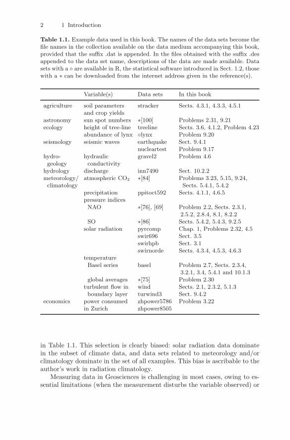
The observations used in this book as examples comprehend climatedata (long-term records of temperature, pressure and radiation), hydro-meteorological data (precipitation events), micro-meteorological data (windspeeds measured in the atmospheric boundary layer), soil parameters, seismo-grams, and hydrological discharge records. The example data sets are given

2 1 Introduction

Table 1.1. Example data used in this book. The names of the data sets become thefile names in the collection available on the data medium accompanying this book,provided that the suffix .dat is appended. In the files obtained with the suffix .desappended to the data set name, descriptions of the data are made available. Datasets with a are available in R, the statistical software introduced in Sect. 1.2, thosewith a ∗ can be downloaded from the internet address given in the reference(s).

Variable(s) Data sets In this book

agriculture soil parameters stracker Sects. 4.3.1, 4.3.3, 4.5.1and crop yields

astronomy sun spot numbers ∗[100] Problems 2.31, 9.21ecology height of tree-line treeline Sects. 3.6, 4.1.2, Problem 4.23

abundance of lynx lynx Problem 9.20seismology seismic waves earthquake Sect. 9.4.1

nucleartest Problem 9.17hydro- hydraulic gravel2 Problem 4.6geology conductivity

hydrology discharge inn7490 Sect. 10.2.2meteorology/ atmospheric CO2 ∗[84] Problems 3.23, 5.15, 9.24,climatology Sects. 5.4.1, 5.4.2

precipitation ppitoct592 Sects. 4.1.1, 4.6.5pressure indicesNAO ∗[76], [69] Problem 2.2, Sects. 2.3.1,

2.5.2, 2.8.4, 8.1, 8.2.2SO ∗[86] Sects. 5.4.2, 5.4.3, 9.2.5

solar radiation pyrcomp Chap. 1, Problems 2.32, 4.5swir696 Sect. 3.5swirhpb Sect. 3.1swirnorde Sects. 4.3.4, 4.5.3, 4.6.3

temperatureBasel series basel Problem 2.7, Sects. 2.3.4,

3.2.1, 3.4, 5.4.1 and 10.1.3global averages ∗[75] Problem 2.30

turbulent flow in wind Sects. 2.1, 2.3.2, 5.1.3boundary layer turwind3 Sect. 9.4.2

economics power consumed zhpower5786 Problem 3.22in Zurich zhpower8505

in Table 1.1. This selection is clearly biased: solar radiation data dominatein the subset of climate data, and data sets related to meteorology and/orclimatology dominate in the set of all examples. This bias is ascribable to theauthor’s work in radiation climatology.

Measuring data in Geosciences is challenging in most cases, owing to es-sential limitations (when the measurement disturbs the variable observed) or

1.1 Data in Geosciences: for Example, Surface Solar Radiation Records 3

limitations in the instruments, data acquisition systems and/or observationalregions or periods, which can deteriorate the quality of the data. Known lim-itations and other (possibly unknown) shortcomings in a data set have to beaccounted for when observations are used in Geosciences and consequently,introductions to the measurement of all data sets used in this book shouldbe given. However, even abbreviated introductions are beyond the scope ofthis book, except for the following three examples:

1. Sect. 9.4.1 introduces the measurement of seismic waves. Seismic wavesare tiny vibrations of the rock that can be recorded by seismometers.They are caused by an earthquake or an explosion, or, as backgroundnoise in a record, by natural phenomena such as ocean waves.

2. Sect. 9.4.2 introduces the measurement of velocities in a turbulent flowin the atmospheric boundary layer.

3. This section introduces the measurement of solar radiation at the surfaceof the earth.

Solar radiation measurements are more delicate than those of meteorologicalvariables such as temperature, precipitation, etc., seeing that radiation in-struments are less stable over longer periods (years) than thermometers, raingauges, etc. Nevertheless, maintenance problems and problems arising fromchanges in (i) the technology of sensors or data acquisition systems and/or(ii) the measuring sites are shared by most long-term measurements of mete-orological variables. Therefore, conclusions drawn from the discussion of solarradiation records also apply to other climate records, e.g., that changes in theobserved values due to changes in the measurement have to be compensatedwhen the data are used for climate change studies.

Solar radiation intercepted by our planet will either be absorbed or re-turned to space by scattering and reflection. Solar radiation is (i) scatteredand reflected by clouds, dry air molecules, water vapour and aerosols in theatmosphere and (ii) reflected by the surface. The absorbed part of the solarradiation (242 Wm−2 (watt per square meter) on the average over the globe,obtained as 71 % (the planetary albedo is 29 % [148]) of 341 Wm−2 (1/4of the solar constant [53]), all values are approximations) is the source ofenergy which drives the processes in the atmosphere and the oceans. Com-pared to this large amount of energy, the flux of heat generated in the interiorof the earth (mostly from radioactive decay) through the earth’s surface isnegligible on the global average. Although being small, the earth’s internalheat fuels convection in its mantle (the layer below its crust) and thus drivesplate-tectonics which — over geological periods — allocates oceans and con-tinents, as described in Sect. 9.4.1. Therefore, solar radiation absorbed in theatmosphere and at the surface of the earth is the primary energy source forlife on our planet which is shaped by processes driven by its internal heat.

Solar radiation absorbed by our planet can be calculated from the compo-nents in the radiation budget at the top of the atmosphere: the earth absorbsand reflects solar radiation incident at the top of the atmosphere and re-

4 1 Introduction

emits the exhaust heat in the form of terrestrial radiation back into space,since it is in radiative equilibrium with the sun and space: incoming andoutgoing radiative fluxes balance each other on condition that no energy isstored/released by heating or cooling the oceans or as latent heat in/fromthe ice and snow masses. As a contrasting aside: Jupiter radiates more en-ergy in space than it receives from the sun. The source of its internal heatis (along with radioactive decay and the tides generated by its satellites)gravitational contraction (when a gravitating object contracts, gravitationalpotential energy is converted into heat).

The radiative fluxes at the top of the atmophere were measured fromspace, using instruments mounted on satellites, in the Earth Radiation Bud-get Experiment (ERBE) over the period from November 1984 through toFebruary 1990. Measuring radiative fluxes in space is a formidable task since(i) instruments have to be built which can be operated in space and, underthe rough conditions prevailing there, will remain stable over relatively long(a few years) periods, since a re-calibration is too costly (ii) the instrumentshave to be mounted on appropriate satellites and (iii) data acquisition andarchival systems have to be maintained ([8], [7]). A continuation (with im-proved instruments) of the ERBE records is provided by the Clouds and theEarth’s Radiant Energy System (CERES) [127].

Measuring solar radiation at the surface and maintaining a network ofmeasuring stations over decades is a task even more difficult than measuringradiative fluxes at the top of the atmosphere. This task can be accomplishedon condition that

1. a consensus has been reached on the world standard maintained by theworld radiation centre (WRC/PMOD) [52] which is then used to cali-brate the reference instruments (secondary standards) maintained by theorganisations (in the majority of cases the national weather services) thatmeasure solar radiation

2. instruments measuring solar radiation are periodically calibrated againstthe secondary standards

3. measurements are guided by best practise recommendations regardingthe installation of calibrated instruments, the maintenance schemes, thedata acquisition systems and the data archival procedures ([57], [94])

4. recommendations for the operational measurements account for differ-ences in climatic regions and are adapted in accordance with the develop-ment of technology without inducing systematic changes in the measuredrecords (counter examples are given in Fig. 2.19)

5. the manned or automated stations (sites) where the instruments aremounted and their neighbourhood remain unchanged over decades

6. the measurements at a site are representative for a larger region, and7. the data archives are maintained over a substantially long period.

Solar radiation records measured under these conditions are homogeneousin space and time: spatial and temporal variations in the data are not due

1.1 Data in Geosciences: for Example, Surface Solar Radiation Records 5

to changes in the observational system. The conditions enumerated aboveestablish standard procedures for the observation of radiative fluxes and alsofor the subsequent data processing and archiving.

The first international standards for observing meteorological variables(e.g., temperature, precipitation, pressure) were introduced in the secondhalf of the 19th century. Observations made with instruments prior to ap-proximately 1860 were less standardised and are therefore often called earlyinstrumental records. The reconstruction of a homogeneous climatologicalseries of, e.g., monthly values, from early instrumental records is a delicatetask. An example is given in Sect. 2.3.4.

Climate records obtained using standard observational procedures are ho-mogenous and thus allow for monitoring climate change. Often, however, cli-mate records are afflicted with inhomogeneities. Inhomogeneities stem froma variety of sources, often they are due to the deficiencies and changes enu-merated in [82]. Climate data that are not homogenous can be adjusted usingprocedures as recommended in [46] or [109]. This difficult task is best done bythe scientist responsible for the measurements since he/she has access to thestation history or the meta data, i.e., the description of the measurements inthe diary kept at the measuring site.

If no detailed station history is available then inhomogeneities (yet notall) can be detected using statistical methods such as those introduced in[66], [59], [88] and [140], or they can be found in relevant plots. In Fig. 2.19for example, the amplitudes of the fluctuations in the differences in solarradiation recorded at neighbouring stations decrease abruptly, in the years1975 and 1980, possibly due to the introduction of automated observations.Subsequent to the detection of such inhomogeneities, an adjustment remainsdifficult.

As a substitute for an adjustment, climate data can be flagged as doubtfuldue to errors and/or inhomogeneities. For example, the solar radiation data inthe Global Energy Balance Archive (GEBA) [59] and also those measured atthe stations of the Baseline Surface Radiation Network (BSRN) [103] undergorigorous quality checks to assure high accuracy as well as homogeneity inthe data, a prerequisite for regression analyses such as those performed inSects. 3.1 and 3.5 to estimate decadal changes in these records ([58], [152]).Due to the quality checks applied, the data in the GEBA and BSRN are, whenused in conjunction with measurements of the radiative fluxes at the top ofthe atmosphere, also suitable for calculating a more accurate disposition ofsolar radiation in the earth-atmosphere system ([3], [150]).

It remains to take a closer look at the measurement of solar radiation atthe surface of the earth which stands in this book representatively for themeasurement of meteorological variables. Solar radiation is measured usingeither a pyrheliometer or a pyranometer. A pyrheliometer is an instrumentdesigned to measure the direct-beam solar radiation. Its sensor is orientedperpendicular to the direction of the sun and is inserted in a tube such that

6 1 Introduction

it intercepts radiation only from the sun and a narrow region of the skyaround the sun. Observations are made when the sky is clear. The quantitymeasured is called direct radiation. Pyrheliometer data are used to study theextinction of solar radiation in an atmosphere free of clouds.

Pyranometers measure the solar radiation from the sun and sky incidenton a horizontal surface. They measure continuously and are exposed to allkinds of weather. Hence, the detector is shielded by a glass dome which,notwithstanding, only transmits radiation in wavelengths between 0.3 and2.8 µm, micrometer, 1 µm = 10−6 m). The glass dome has to be kept cleanand dry. The detector has at least two sensing elements, one blackened suchthat most of the incident solar radiation is absorbed and the other coatedwith a white paint such that most radiation is reflected (or placed in shadeto avoid solar radiation). The temperature difference between these elementsis approximately proportional to the incident radiation. Annual calibrationsare recommended because the responsivity of pyranometers deteriorates overtime. The meteorological variable measured with a pyranometer is calledglobal radiation or shortwave incoming radiation (SWIR).

Errors in pyranometer measurements may arise from various sources, of-ten from instrumental deficiencies during the measurement. There are ran-dom errors and systematic errors. A random error is zero in the mean ofthe measurement period, a systematic error has a non-zero mean. An exam-ple of a systematic error with a time-dependent mean is the error producedby a drifting sensitivity of an instrument. Systematic errors can be detectedand possibly corrected, provided that a detailed station history is available.Random errors cannot be corrected, but their statistical structure can betaken into account when the data are used, as demonstrated in Sects. 3.1.1,3.5, 4.6.3, and 4.6.5. With a good instrument the random error of a singlepyranometer measurement is 2% of the measured value.

The maintenance of the instruments, their installation and the data ac-quisition system is crucial to the quality of the measurements. Errors (sys-tematic and/or random) can therefore not be excluded. Errors in the singlepyranometer readings propagate to the hourly, daily, monthly, and yearlymeans aggregated consecutively from the original data. How much influencedoes maintenance have on the quality of pyranometer data? This questionwas investigated in a long-term pyranometer comparison project jointly per-formed by the Federal Office for Meteorology and Climatology (MeteoSwiss)and the Swiss Federal Institute of Technology (ETH), both in Zurich. In thisproject, the shortwave incoming radiation was measured by both institutionsfrom January 1, 1989 through to December 30, 1992 at the same (Reckenholz)station, but completely independently. The instruments used in the exper-iment were both Moll-Gorczynsky-type thermoelectric pyranometers, madethough by different manufacturers. The installation of the instruments, themaintenance schemes, and the data acquisition systems were chosen delib-

1.1 Data in Geosciences: for Example, Surface Solar Radiation Records 7

Table 1.2. A pyranometer comparison experiment was performed at Zurich-Reckenholz (8031′E, 47025′N, 443 m a.m.s.l.) station jointly by the Federal Officefor Meteorology and Climatology (MeteoSwiss) and the Swiss Federal Institute ofTechnology (ETH).

Pyranometer MeteoSwiss ETH

manufacturers Kipp Swissteco

calibrated with the MeteoSwiss at the World Radiationstandard instrument Centre in Davos

installation instrument instrumentlightly ventilated neither ventilatedbut not heated nor heated

data acquisition A-net Allgomatic(MeteoSwiss standard)

averaged over 10 minutes 5 minutes

maintenance daily weekly

erately not to be identical (Table 1.2) to simulate the distinct pyranometerinstallations of the institutions that measure and publish SWIR data [58].

From the Reckenholz measurements, hourly and daily averages were cal-culated consecutively. These daily averages are stored in the following format

89 1 1 13 12

89 1 2 18 18

...

92 12 30 18 18

in the file /path/pyrcomp.dat. This is an example of a text file containing atable of data as, for each day, it contains a line with five values. The first threerepresent time of the measurement as year, month and day. The fourth valueis the daily mean of SWIR calculated from the MeteoSwiss measurements,and the fifth, the daily mean calculated from the ETH measurements. Theunit of the radiation values is Wm−2. Missing data are represented as NA

(not available). A description of the pyranometer data is given in the file/path/pyrcomp.des.

This convention is used for all example data sets: the file /path/name.dat

contains the data, the file /path/name.des their description. Please follow theinstructions in Problem 1.1 to read the example data sets from the datamedium accompanying this book.

The example data sets stored on the data medium were prepared in theyears 2003 and 2004 immediately preceding the production of this book.Updated versions of the example data sets originating from the internet maybe available from the sites referenced. You are encouraged to visit these sites

8 1 Introduction

and possibly to reproduce the statistical analyses with the updated data sets.Then, however, you will obtain slightly different results.

Having thus transferred an example data set to your computer, you mayperform a statistical analysis using R. As an example, in Sects. 1.3 and 1.4,daily averages from the pyranometer comparison experiment described aboveare analysed using R. R is introduced in the next section.

1.2 R

R is a programming language for the graphical representation and statisticalanalysis of data. Expressions in R usually contain R functions; an example isgiven in the following line

result <- function(arg1, arg2, ...) #comment

In this example, result and arg1, arg2, ... are R objects. R objects can beatomic or non-atomic. Typical non-atomic objects are R vectors and matrices.R functions and objects R are not, however, explained in detail. R and also

a description of R are available from [114]; to obtain the language referencestart the R help system by typing help.start() in R. R is available for mostoperating systems. Depending on the operating system, start an internetbrowser before invoking the R help system.

Assuming you have access to R, take advantage of the opportunity andwork through this section. With the following expressions

rholzdayfilename <- "/path/pyrcomp.dat" #filename

rholzdayformat <- list(year=0,month=0,day=0,smi=0,eth=0) #format

rhd <- scan(rholzdayfilename, rholzdayformat) #read file

you can read all values from the file /path/pyrcomp.dat into rhd. The R ob-ject rhd is a collection of five parallel vectors: rhd$year, rhd$month, rhd$day,

rhd$smi, rhd$eth.In R, the result of operators (functions) depends on the type of operands

(arguments). For example, R delivers the result 3, if you typeseven <- 7

four <- 4

seven - four

However, if the operands are vectors, R checks if they have the same lengthand then performs the same operation on all values. Thus, the result is avector again. In the following example,

difsmieth <- rhd$smi - rhd$eth

the first value in the vector rhd$eth is subtracted from the first value inrhd$smi with the result stored as the first value in difsmieth. This operationis repeated until the operand vectors are processed to their entire length.

If an R expression contains an R function, the type of the resulting objectdepends on the function and its arguments. For example, when a table ofdata is read with scan() and a data format, as in the example above, theresult is a collection of vectors. Is the same result delivered by the R function

1.2 R 9

read.table()? read.table() is often used to read text files containing tablesof data.

The number of values in an R vector is available with the R functionlength(), e.g., as the last day of the pyranometer comparison experiment isDecember 30, 1992, and as 1992 is a leap year

length(rhd$eth)

[1] 1460

tells you that there are 1460 values in the vector rhd$eth, in accordance withthe duration of the comparison experiment. The vector values are indexed,e.g., the R expressions

rhd$smi[1:40]

[1] 13 18 39 55 22 20 15 33 20 16 30 49 73 70 48 18 24 48 19 59

[21] 56 25 11 48 25 NA 31 72 54 29 27 70 65 35 79 79 96 NA 59 NA

rhd$eth[1:40]

[1] 12 18 35 47 21 19 15 32 20 16 29 44 57 58 45 17 24 45 18 55

[21] 52 24 11 46 20 38 30 67 44 29 26 65 62 32 75 75 90 63 53 39

write out the first 40 values in rhd$smi and rhd$eth. On January 1st, 1989, thefirst day of the experiment, the MeteoSwiss pyranometer measured 13 Wm−2,1 Wm−2 more than the ETH instrument. The next day both measurementswere identical. On January 26th, the MeteoSwiss measurement was not avail-able. How many days with identical values occurred in the pyranometer com-parison experiment? The expressions

smieth <- rhd$smi[(1:length(rhd$smi))[(rhd$smi == rhd$eth)]]

ethsmi <- rhd$eth[(1:length(rhd$eth))[(rhd$eth == rhd$smi)]]

generate two R vectors, which contain only identical daily values from theMeteoSwiss and ETH instruments. Both vectors are identical. With the ex-pressions

length(smieth)

smieth

the length of the vector smieth and its values are written out. smieth con-tains missing values, because (i) the vectors with the measurements containmissing values and (ii) the equality condition (rhd$smi == rhd$eth), in theexpressions above, delivers T (true), even if the values compared are NAs, i.e.,if one or both values are missing. To exclude these cases, use the R functionis.na(), which results in T (true) or F (false) and is negated with !. Using

smi1 <- rhd$smi[(1:length(rhd$smi))[(!is.na(rhd$smi))]]

eth1 <- rhd$eth[(1:length(rhd$eth))[(!is.na(rhd$eth))]]

smi2 <- rhd$smi[(1:length(rhd$smi))

[(!is.na(rhd$smi))&(!is.na(rhd$eth))]]

eth2 <- rhd$eth[(1:length(rhd$eth))

[(!is.na(rhd$eth))&(!is.na(rhd$smi))]]

the vectors smi1, eth1, smi2 and eth2 are generated. The vector smi1 con-tains the MeteoSwiss measurements for these days only, when the value isnot missing. The length of smi1 is 1358, i.e., MeteoSwiss measurements are

10 1 Introduction

missing for 102 out of 1460 days. The figures for the ETH measurements are28 out of 1460 days. The vector smi2 contains the MeteoSwiss pyranometervalues for days when both measurements are available. The length of thisvector is 1330, i.e., during the comparison period there are 1330 days withboth the MeteoSwiss and ETH measurement. Consequently, the two condi-tions above delivering smi2 and the comparison (rhd$smi == rhd$eth) in theexpressions

smieth1 <- rhd$smi[(1:length(rhd$smi))[(rhd$smi == rhd$eth)&

(!is.na(rhd$smi))&(!is.na(rhd$eth))]]

ethsmi1 <- rhd$eth[(1:length(rhd$eth))[(rhd$eth == rhd$smi)&

(!is.na(rhd$eth))&(!is.na(rhd$smi))]]

are needed to obtain the result, that only for 215 out of 1460 days the sameshortwave incoming radiation value was obtained from the measurements.

Another strength of R is the graphical representation of data. You canchoose where your graphic device will be generated, e.g., with

postscript(file="fig11.ps",horizontal=F,width=4,height=4)

the plots are written to a postscript-file. Then, you may choose how the plotsare depicted. With

par(mfrow=c(1,3))

you receive, e.g., three plots side by side, as shown in Fig. 1.1. Withdev.off()

the graphic device closes (R functions dev.xxx() provide control over multiplegraphics devices). Do not forget to close a postscript-file when the graphicaldescription is complete.

The MeteoSwiss and ETH pyranometer daily values, made available asR vectors in this section, are analysed in the next section with mean() andvar(), both R functions, under the usual statistical assumptions.

1.3 Independent Identically Distributed (Iid.) RandomVariables

In this section, the basics of statistical data analysis are reviewed. As anexample, the pyranometer daily values are analysed in Sects. 1.3.1 and 1.3.3under the assumptions that they are (i) identically distributed and (ii) in-dependent from one day to the next or previous or any other following orpreceding day, i.e., that they are iid. The statistical analysis under the iid. as-sumptions is reviewed in Sect. 1.3.2. The pyranometer daily values, however,are not iid., as follows from a discussion in Sect. 1.3.4.

1.3.1 Univariate Analysis of the Pyranometer Data

As shown in Sect. 1.2, the data resulting from the pyranometer comparisonexperiment are erroneous. Do the errors afflict the histograms of the data?The R expressions

1.3 Independent Identically Distributed (Iid.) Random Variables 11

MeteoSwiss

Fre

quen

cy

0 100 250

020

4060

8010

012

0

ETH

Fre

quen

cy

0 100 250

020

4060

8010

012

0

MeteoSwiss − ETH

Fre

quen

cy

0 20 60

010

020

030

040

050

060

0

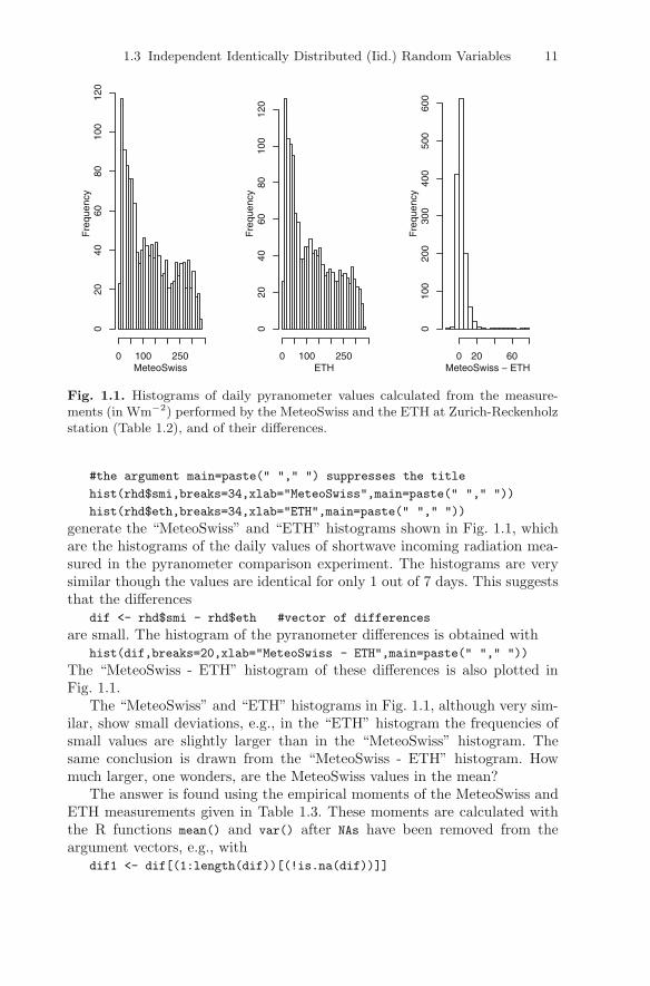
Fig. 1.1. Histograms of daily pyranometer values calculated from the measure-ments (in Wm−2) performed by the MeteoSwiss and the ETH at Zurich-Reckenholzstation (Table 1.2), and of their differences.

#the argument main=paste(" "," ") suppresses the title

hist(rhd$smi,breaks=34,xlab="MeteoSwiss",main=paste(" "," "))

hist(rhd$eth,breaks=34,xlab="ETH",main=paste(" "," "))

generate the “MeteoSwiss” and “ETH” histograms shown in Fig. 1.1, whichare the histograms of the daily values of shortwave incoming radiation mea-sured in the pyranometer comparison experiment. The histograms are verysimilar though the values are identical for only 1 out of 7 days. This suggeststhat the differences

dif <- rhd$smi - rhd$eth #vector of differences

are small. The histogram of the pyranometer differences is obtained withhist(dif,breaks=20,xlab="MeteoSwiss - ETH",main=paste(" "," "))

The “MeteoSwiss - ETH” histogram of these differences is also plotted inFig. 1.1.

The “MeteoSwiss” and “ETH” histograms in Fig. 1.1, although very sim-ilar, show small deviations, e.g., in the “ETH” histogram the frequencies ofsmall values are slightly larger than in the “MeteoSwiss” histogram. Thesame conclusion is drawn from the “MeteoSwiss - ETH” histogram. Howmuch larger, one wonders, are the MeteoSwiss values in the mean?

The answer is found using the empirical moments of the MeteoSwiss andETH measurements given in Table 1.3. These moments are calculated withthe R functions mean() and var() after NAs have been removed from theargument vectors, e.g., with

dif1 <- dif[(1:length(dif))[(!is.na(dif))]]

12 1 Introduction

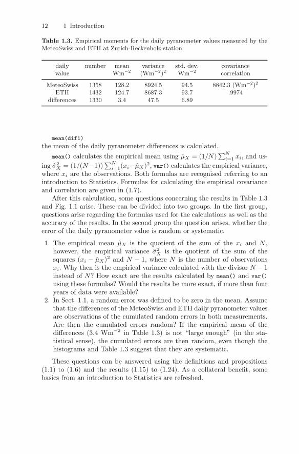
Table 1.3. Empirical moments for the daily pyranometer values measured by theMeteoSwiss and ETH at Zurich-Reckenholz station.

daily number mean variance std. dev. covariancevalue Wm−2 (Wm−2)2 Wm−2 correlation

MeteoSwiss 1358 128.2 8924.5 94.5 8842.3 (Wm−2)2

ETH 1432 124.7 8687.3 93.7 .9974differences 1330 3.4 47.5 6.89

mean(dif1)

the mean of the daily pyranometer differences is calculated.mean() calculates the empirical mean using µX = (1/N)

∑Ni=1 xi, and us-

ing σ2X = (1/(N−1))

∑Ni=1(xi−µX)2, var() calculates the empirical variance,

where xi are the observations. Both formulas are recognised referring to anintroduction to Statistics. Formulas for calculating the empirical covarianceand correlation are given in (1.7).

After this calculation, some questions concerning the results in Table 1.3and Fig. 1.1 arise. These can be divided into two groups. In the first group,questions arise regarding the formulas used for the calculations as well as theaccuracy of the results. In the second group the question arises, whether theerror of the daily pyranometer value is random or systematic.

1. The empirical mean µX is the quotient of the sum of the xi and N ,however, the empirical variance σ2

X is the quotient of the sum of thesquares (xi − µX)2 and N − 1, where N is the number of observationsxi. Why then is the empirical variance calculated with the divisor N − 1instead of N? How exact are the results calculated by mean() and var()

using these formulas? Would the results be more exact, if more than fouryears of data were available?

2. In Sect. 1.1, a random error was defined to be zero in the mean. Assumethat the differences of the MeteoSwiss and ETH daily pyranometer valuesare observations of the cumulated random errors in both measurements.Are then the cumulated errors random? If the empirical mean of thedifferences (3.4 Wm−2 in Table 1.3) is not “large enough” (in the sta-tistical sense), the cumulated errors are then random, even though thehistograms and Table 1.3 suggest that they are systematic.

These questions can be answered using the definitions and propositions(1.1) to (1.6) and the results (1.15) to (1.24). As a collateral benefit, somebasics from an introduction to Statistics are refreshed.

1.3 Independent Identically Distributed (Iid.) Random Variables 13

1.3.2 Unbiased and Consistent Estimators, Central LimitTheorem

The daily MeteoSwiss and ETH pyranometer values analysed above werecalculated from the measurements made during the Reckenholz comparisonexperiment. Since error free measurements are impossible, it is assumed thatthe daily MeteoSwiss and ETH values are random, i.e., observations of ran-dom variables. Hence, also their differences are random. Under this basicassumption, the empirical moments in Table 1.3 are examples of estimates,as defined in (1.1).

The estimate uX is an observed value of the estimatorUX = g(X1, . . . , XN ), on condition that uX = g(x1, . . . , xN ) iscalculated with the formula g from the observations x1, . . . , xN

of the random variables X1, . . . , XN .

(1.1)

In (1.1), the estimator UX is a functional of the (joint) distribution of therandom variables X1, . . . , XN , with the distribution of g(X1, . . . , XN ) beingconcentrated in uX . A functional is a mapping (usually a formula), whichassigns a real number to each function in a set of functions. The concept ofconcentration is mentioned in the remarks to the Chebyshev inequality (1.17)and discussed in an introduction to Statistics.

Often UX is written as uX . Once this simplification has been made, itbecomes clear from the context whether uX is an estimate or an estimator.Estimates may be found using different methods, e.g., moment, least squaresand maximum likelihood estimates are known from an introduction to Statis-tics.

For instance, the empirical means in Table 1.3, calculated from the dailySWIR observations xi, are estimates as defined in (1.1). In this example,the formula g is the arithmetic mean, and the estimate is calculated usinguX = (1/N)

∑Ni=1 xi from the observed values xi. According to definition

(1.1), uX is the observed value of the estimator UX = (1/N)∑N

i=1Xi, andXi is the theoretical daily SWIR at day i, i.e., a random variable.

With definition (1.1) alone, the questions in the remarks to Table 1.3 can-not be answered. For example, intuition suggests that more accurate meanscould be calculated if more than four years of data were available. This can-not be shown to be either true or false using only (1.1). To find the answersto this and the other questions in the remarks to Table 1.3, some constrainingproperties of the theoretical SWIR Xi at day i are therefore assumed. Theusual statistical assumptions are found in (1.2).

Each observation delivers a possible value xi of the randomvariable Xi. The set of the xi is a random sample provided that

1. an arbitrary number of observations is takenunder identical conditions, and

2. each observation is taken independently from one another.

(1.2)

14 1 Introduction

Under these assumptions, the estimate uX in (1.1) is calculated using g fromN observations xi, which are possible values of N identically distributed, andindependent random variables Xi. The identical distributions of the Xi arerequired in (1.2,1), and the independence of the Xi in (1.2,2). Random vari-ables Xi with the properties required in (1.2) are said to be independent andidentically distributed (iid.). Therefore, the assumptions in (1.2) are callediid. assumptions.

Under the iid. assumptions, the estimator UX = g(X1, . . . , XN ) as definedin (1.1) is a function of N random variables Xi, which are iid. Hence, one caneasily calculate its moments EUX and VarUX , using the rules in (1.15), if (i)the estimator is linear (a weighted sum of theXi) and (ii) the expectation EXi

and the variance VarXi of the Xi is known. If, in addition, the distributionof Xi is known, the distribution of UX can then be calculated.

As an example, the moments of the mean of a random sample are calcu-lated below. Assuming that the xi are iid., and also assuming that µX is theexpectation ofXi, that σ2

X is the variance ofXi and µX is the arithmetic meanof the xi, you obtain with (1.15,4) EµX = (1/N)

∑Ni=1 EXi = (1/N)NEXi =

µX and with (1.15,6) and (1.16,4) VarµX = (1/N2)∑N

i=1 VarXi = (1/N2)N×VarXi = (1/N)σ2

X .The mean of a random sample is an example of an estimator without bias,

which is defined in (1.3).

An estimator UX has no bias (is unbiased, bias-free), on conditionthat EUX = uX , with uX being the unknown theoretical value.

(1.3)

If the Xi are iid. as required in (1.2), uX in (1.3) is often an unknown pa-rameter in the distribution of the Xi. For instance, uX stands for µX or σ2

X ,assuming that Xi is normally distributed, or for λX , assuming that Xi isPoisson distributed. As another example, it is shown in Problem 1.4, thatthe empirical variance is an unbiased estimator of the theoretical variance ifthe Xi are iid., since Eσ2

X = E((1/(N−1))

∑Ni=1(xi− µX)2

)= σ2

X . However,σ2

X = (1/N)∑N

i=1(xi − µX)2)

is not an unbiased estimate for the varianceof a random sample. If an unbiased estimator is used, you can be certainthat an unknown theoretical value is neither over- nor underestimated in themean, when the estimates are calculated from many samples taken. This isa desirable property.

Another desirable property of an estimator is its consistency as definedin (1.4). If a consistent estimator UX is used, then the probability that theabsolute difference of the estimate uX and the true value uX , |uX−uX |, beingless than a small ε, comes close to 1 for an arbitrarily large N . Consequently,in the mean of many random samples, the estimates become more accurateif the sample size N increases. For N → ∞, VarµX → 0, since the estimatoris defined for N = 1, 2, 3, . . ..

1.3 Independent Identically Distributed (Iid.) Random Variables 15

It is assumed that UX = g(X1, . . . , XN ) is an unbiased estimatordefined for N = 1, 2, 3, . . .. If its variance E(UX − uX)2 → 0 forN → ∞, then, from the Chebyshev inequality (derived in (1.17)),Pr(|UX − uX | < ε)= 1 − Pr

(|UX − uX | ≥ ε)→ 1 for N → ∞ and

for each ε > 0, is obtained.Then UX is said to be a consistent estimator.

(1.4)

For example, the mean µX of a random sample is a consistent estimatorfor the expectation EX = µX of the Xi, since EµX = µX and VarµX =E(µX −EµX)2 = E(µX −µX)2 = (1/N)σ2

X , σ2X = VarX, the variance of the

Xi, as shown in the remarks to (1.2). Thus µX is unbiased and VarµX → 0as N → ∞.

In the case of the pyranometer comparison experiment, it is concludedfrom (1.4) that the estimated means in Table 1.3 would be more accurateif the experiment had been performed over a longer period than the fouryears from 1989 to 1992. This is true under the assumption that the dailypyranometer values are in agreement with the iid. assumptions in (1.2).

This completes the answers to the first group of questions in the remarksto Table 1.3. The remaining question in the second group, i.e., whether thedifferences in the pyranometer daily values are due to random errors in bothmeasurements, can only be answered if the probability distribution of themean of the daily differences is known. Using this distribution, a confidenceinterval for the mean can be calculated. If then the confidence interval con-tains the value 0, the cumulative error is assumed to be random. Anotherpossibility is to perform a statistical test using the distribution of the meanof the daily differences. Is it possible to assess this distribution?

Under the iid. assumptions in (1.2), it is possible to derive the probabilitydistribution of an estimator as defined in (1.1) if the estimator, i.e., theformula g, is not too complicated and if the probability distribution of the Xi

is known. This derivation is straightforward, because the distribution F (y) ofthe function Y = g(X1, . . . , XN ) of N random variables Xi can be calculatedin (1.5)

F (y) =∫

(N). . .

∫By

(f(x1, x2, . . . , xN )

)dx1 . . .dxN

=∫

(N). . .

∫By

(f(x1)f(x2) . . . f(xN )

)dx1 . . .dxN (1.5)

By = (x1, . . . , xn)|g(x1, . . . , xn) ≤ yas the N -multiple integral of the N -times product of the density f(xi) ofthe Xi, if the Xi are independent and identically distributed with F (xi),i = 1, . . . , N .

For instance, from (1.18) to (1.24) it is concluded that the mean of arandom sample µX = (1/N)

∑Ni=1 xi is normally distributed with EµX = µX