PNNL-16925

Hanford Soil Inventory Model (SIM) Rev. 2 User’s Guide B. C. Simpson R. A. Corbin M. J. Anderson C. T. Kincaid September 2007 Prepared for the U.S. Department of Energy under Contract DE-AC05-76RL01830

DISCLAIMER This report was prepared as an account of work sponsored by an agency of the United States Government. Neither the United States Government nor any agency thereof, nor Battelle Memorial Institute, nor any of their employees, makes any warranty, express or implied, or assumes any legal liability or responsibility for the accuracy, completeness, or usefulness of any information, apparatus, product, or process disclosed, or represents that its use would not infringe privately owned rights. Reference herein to any specific commercial product, process, or service by trade name, trademark, manufacturer, or otherwise does not necessarily constitute or imply its endorsement, recommendation, or favoring by the United States Government or any agency thereof, or Battelle Memorial Institute. The views and opinions of authors expressed herein do not necessarily state or reflect those of the United States Government or any agency thereof.

PACIFIC NORTHWEST NATIONAL LABORATORY operated by BATTELLE

for the UNITED STATES DEPARTMENT OF ENERGY

under Contract DE-AC05-76RL01830

Printed in the United States of America

Available to DOE and DOE contractors from the Office of Scientific and Technical Information,

P.O. Box 62, Oak Ridge, TN 37831-0062; ph: (865) 576-8401 fax: (865) 576-5728

email: reports@adonis.osti.gov

Available to the public from the National Technical Information Service, U.S. Department of Commerce, 5285 Port Royal Rd., Springfield, VA 22161

ph: (800) 553-6847 fax: (703) 605-6900

email: orders@ntis.fedworld.gov online ordering: http://www.ntis.gov/ordering.htm

This document was printed on recycled paper.

______________________________ (a) Vivid Learning Systems, Inc., Pasco, Washington (b) Columbia Energy and Environmental Services, Inc., Richland, Washington

PNNL-16925

Hanford Soil Inventory Model (SIM) Rev. 2 User’s Guide B. C. Simpson(a)

R. A. Corbin(b)

M. J. Anderson(a)

C. T. Kincaid September 2007 Prepared for the U.S. Department of Energy under Contract DE-AC05-76RL01830 Pacific Northwest National Laboratory Richland, Washington 99352

Summary

This document provides a user’s guide for Hanford Soil Inventory Model (SIM) Rev. 2. and the software portfolio developed to maintain it. The Hanford SIM application computes waste discharges composed of 75 analytes at 377 waste sites (liquid disposal, unplanned releases, and tank farm leaks) over an operational period of approximately 50 years.

A computer model capable of calculating inventories and the associated uncertainties as a function of time was identified to address the needs of the Remediation and Closure Science (RCS) Project. This user’s guide is a companion document to a report on the requirements, conceptual model, simulation, methodology, testing, and quality assurance associated with Hanford SIM Rev. 2.

To estimate mass-balanced contaminant inventories and their uncertainties for the Hanford Site post-closure setting, a stochastic simulation method (a Monte Carlo-type calculation) was selected to provide estimates of inventory and uncertainty. The Open Crystal Ball (OCB) statistical package was selected in 2002 for application in this model.

The principal outcome of this effort is the upgrade of the software suite to the latest versions of OCB and Crystal Ball (CB), to make the modeling capability available to the broader technical community. This version of Hanford SIM requires the user to have Crystal Ball v7.x and Microsoft Office 2003. This model will be available to U.S. Department of Energy (DOE) offices, DOE contractors, and those wishing to review the technical basis for and simulation of inventories appearing in Hanford assessments.

The design of Hanford SIM is highly modular, with separate data input (Microsoft Excel) and calculation engine (OCB.dll) files administered through an interface application that acquires the inputs, manages the data reporting, and creates the output files. Each data input is considered an independent variable; therefore, the waste stream composition/properties and waste stream discharge histories for the waste disposal sites can be examined and developed using a variety of source data (e.g., historical process data, tank waste modeling) and assumptions without affecting other variables.

iii

v

Terms/Acronyms

AMD advanced micro device CB Crystal Ball DVD digital video disc GB gigabyte GHz gigahertz HDW Hanford Defined Waste (Model) OCB Open Crystal Ball LHS Latin hypercube sampling MB megabyte ML megaliter PNNL Pacific Northwest National Laboratory RAM random access memory RCS Remediation and Closure Science (Project) SIM Soil Inventory Model UPR unplanned release UPS uninterruptible power supply USB universal serial bus

Contents Summary ............................................................................................................................................ iii Terms/Acronyms ................................................................................................................................ v 1.0  Introduction ............................................................................................................................. 1.1 

1.1  Program Development .................................................................................................... 1.1 1.2  Overview of Software Capabilities ................................................................................ 1.1 1.3  Hardware and Software Requirements ........................................................................... 1.1 

1.3.1  Hardware Requirements .................................................................................... 1.1 1.3.2  Software System Requirements ......................................................................... 1.2 

1.4  Program Evolution ......................................................................................................... 1.3 1.5  User’s Guide Organization ............................................................................................. 1.4 

2.0  Model Orientation ................................................................................................................... 2.1 2.1  Installation ...................................................................................................................... 2.1 2.2  Simulation Control ......................................................................................................... 2.1 

2.2.1  Setup Worksheet ................................................................................................ 2.2 2.2.2  Legend Worksheet ............................................................................................. 2.4 

2.3  Input File Preparation, Variable Definition and Parameterization ................................. 2.8 3.0  Input Modification through the Microsoft Excel User Interface ............................................. 3.1 

3.1  Adding or Editing a Site for Inclusion in the Simulation ............................................... 3.1 3.2  Adding or Editing Site Volumes .................................................................................... 3.1 3.3  Adding a Waste Stream Entry ........................................................................................ 3.2 3.4  Defining Analyte Concentrations in a New Waste Stream ............................................ 3.3 3.5  Editing Analytes in Current Hanford SIM Waste Streams ............................................. 3.4 3.6  Adding a Waste Stream Density Definition ................................................................... 3.5 3.7  Determining Correction Factor Values .......................................................................... 3.5 

4.0  Executing a Soil Inventory Model Simulation ........................................................................ 4.1 4.1  Distributed Computing ................................................................................................... 4.4 

4.1.1  Splitting Runs .................................................................................................... 4.4 4.1.2  Merging the Runs .............................................................................................. 4.4 

5.0  Quality Assurance and Error Recovery Guidance ................................................................... 5.1 5.1  Convergence ................................................................................................................... 5.1 5.2  Top 10 Lists .................................................................................................................... 5.4 5.3  Blackbox Test ................................................................................................................. 5.4 5.4  Volume Balance Macro .................................................................................................. 5.5 5.5  Other Quality Assurance and Error Recovery Tests ...................................................... 5.6 

6.0  Hanford SIM Rev. 2 Outputs ................................................................................................... 6.1 6.1  Category (Operable Unit) Workbook Results ................................................................ 6.1 6.2  System Assessment Capability Model Output Files....................................................... 6.1 

vii

viii

6.3  Summary Inventory Spreadsheets .................................................................................. 6.2 6.4  Top 10 Lists Spreadsheets .............................................................................................. 6.2 6.5  Data Migration ............................................................................................................... 6.2 

6.5.1  Input Files .......................................................................................................... 6.2 6.5.2  Output Files ....................................................................................................... 6.3 

7.0  References ............................................................................................................................... 7.1 Appendix – Software Environment Maintenance .............................................................................. A.1 

Figures 2.1 Simulation Control—Setup Worksheet Illustration ................................................................... 2.3 2.2 Legend Identification Matrices—Locations, Analytes, Waste Streams ..................................... 2.5 2.3 Legend Worksheet—Distributed Computing Administration ................................................... 2.6 2.4 Hanford SIM Rev. 2 Dialog Box ............................................................................................... 2.7 3.1 CorrFactors Worksheet Example .............................................................................................. 3.5 4.1 Hanford SIM Rev. 2 User Flow Diagram .................................................................................. 4.2 5.1 Convergence User Interface ....................................................................................................... 5.2 5.2 Convergence Test Output .......................................................................................................... 5.3 6.1 Dialog Example – Successful Migration of Input Data to Database Storage ............................ 6.3 6.2 Dialog Example – Successful Migration of Output Data to Database Storage for 200-E

Ponds Zone ................................................................................................................................ 6.4 

Tables 1.1 Hardware Requirements for Hanford SIM Rev. 2 Operation .................................................... 1.2 2.1 Available Distribution Parameter Definitions, Hanford SIM Rev. 2 ......................................... 2.8 2.2 Proposed Distribution Selection Criteria and Application in Hanford SIM Rev. 2 ................... 2.9 2.3 Hanford SIM Rev. 2 Continuous Distributions ......................................................................... 2.10 3.1 SiteInput Worksheet Example, Hanford SIM Rev. 2 ................................................................. 3.2 3.2 AnalyteInput Worksheet Example, Hanford SIM Rev. 2 ........................................................... 3.3 3.3 DensityInput Worksheet Example, Hanford SIM Rev. 2 ........................................................... 3.5 6.1 Hanford SIM Rev. 2 Output File Label and Number of Rows in Record ................................. 6.4 

1.0 Introduction

The focus of the development and application of a contaminant source term inventory model was to develop a probabilistic approach to estimate comprehensive, mass-balance–based contaminant inventories for the Hanford Site post-closure setting. The outcome of this effort was the Hanford Soil Inventory Model (SIM). This document is a user’s guide for the Hanford SIM Rev. 2 software, which relies on currently available software products including Microsoft Office 2003 and Crystal Ball v7.x.

1.1 Program Development

The inventory quantification effort with regard to vadose zone and groundwater contamination is focused on extending the Hanford Defined Waste (HDW) Model (Agnew et al. 1997; Higley et al. 2004) and other process knowledge to quantify contaminant inventories and uncertainties for liquid waste disposal sites, unplanned releases, and tank leaks that directly received process waste in the 200 Areas of the Hanford Site; and a select number of sites in the 300 Area. The software described here is an updated version of Hanford SIM Rev. 1 published in 2005 (Corbin et al. 2005). As verification that changes to the software have not substantially altered model results, the current software has been used to duplicate the previously published inventories (Corbin et al. 2005) discharged or leaked to the vadose zone.

1.2 Overview of Software Capabilities

The current Hanford SIM application simulates the discharge of 75 analytes at 377 waste sites over an operational period of approximately 50 years. Hanford SIM Rev. 2 provides annual and consolidated inventory and uncertainty estimates for each analyte and waste site, with the capability to group waste site contaminant inventories in a variety of ways. The Monte Carlo calculations can be done in either simple random sampling or Latin hypercube sampling (LHS) (Iman and Conover 1982) with large numbers of iterations.

The Hanford SIM architecture is flexible enough to add/modify waste streams and waste sites as needed or focus the model calculations and analyses on a specific set of years, waste sites, and analytes. Additional post-processing quality assurance, diagnostic, and analytical tools exist as part of the overall system to further evaluate the Hanford SIM results. These capabilities will be discussed in more depth in Section 5 of this user’s guide.

1.3 Hardware and Software Requirements

1.3.1 Hardware Requirements

Using conventional personal computers for this task was desired; thus, several hardware-based challenges impede the execution of the model. These challenges are associated with reading and writing the input data, performing large numbers of computations, and managing the output data. Thus, operation of Hanford SIM is limited predominantly by the amount of available random access memory (RAM) provided in the computer. However, because the Windows XP operating system constrains RAM memory use to 1.3 gigabytes (GB), more RAM above this limit does not enhance performance. Table 1.1 details the minimum and recommended hardware necessary to operate Hanford SIM. The recommended hardware configuration was used for both the development and execution of Hanford SIM Rev. 2.

1.1

Table 1.1. Hardware Requirements for Hanford SIM Rev. 2 Operation

Minimum Required Hardware to Operate/Execute Hanford SIM Rev. 2

Recommended Hardware to Operate/Execute Hanford SIM Rev. 2

Intel Pentium 4 system, with a clock speed of at least 2.53 GHz (Hanford SIM has not been tested on the AMD platform)

Several Intel-based Pentium 4 systems with clock speeds greater than 3.0 GHz

1 GB of RAM 2 GB of RAM 1 GB of free hard drive space 5 GB of free hard drive space Smaller than a 20-in. monitor Greater than a 20-in. monitor PC case operating with the original equipment manufacturer’s installed fan

PC case with room for operating at least 4 case fans Uninterruptible power supplies (UPS)

DVD-R DVD-RW USB mass storage drive

AMD = Advanced micro devices. DVD = Digital video disc. GB = Gigabytes. GHz = Gigahertz. PC = Personal computer. RAM = Random access memory. SIM = Soil Inventory Model. UPS = Uninterruptible power supplies. USB = Universal serial bus.

Computers meeting the minimum requirements can be used to run Hanford SIM, but the run times for the simulations become exceedingly long. A complete converged model run (assuming a typical 2005 model configuration) using the recommended hardware configuration distributed over four computers takes more than 100 hours of chronological time or more than 400 machine-hours of computing time. Therefore, using a single machine with the minimum requirements to execute a full simulation as defined would take in excess of two weeks of continuous operation to complete.

The amount of time necessary to complete a simulation varies as a function of the number of trials, sites, and analytes being evaluated, but other than for relatively simple troubleshooting situations, these models are very demanding with regard to the amount of time they take to perform.

1.3.2 Software System Requirements

These are the minimum software requirements for performing calculations using the current Hanford SIM and its associated infrastructure:

• Windows XP Professional SP21; provides the operating system for the computer.

• Windows.NET 1.11; provides the application environment.

• Crystal Ball2 v7.2; provides the ability to evaluate scenarios using macros as part of the data analysis and quality assurance infrastructure.

1. Software product of Microsoft Corporation, Redmond, Washington. 2. Software product of Decisioneering, Denver, Colorado.

1.2

• Open Crystal Ball2 2.0 (OCB.dll); provides the computational engine to perform the stochastic calculations.

• C# interface (OCBHanford3); administers the simulation by managing inputs and outputs through OCB.

• Microsoft Excel1 2003; user interface for data input/output and analysis.

• Microsoft Excel1 SQL Server 2000; database for configuration control.

A discussion of Hanford SIM requirements, design, and limitations can be found in Anderson et al. (2007). Additionally, the project file contains the Software Requirements Specification and Software Design Document for Hanford SIM Rev. 2.

1.4 Program Evolution

The proof-of-principle software product and its application were documented in Simpson et al. (2001). That product, Hanford SIM Rev. 0, was applied to generate inventory estimates for 46 radionuclides and 27 chemicals from 88 liquid waste disposal sites. These estimates provided uncertainty bounds around the calculated inventory using uncertainties defined in the input data.

The successful outcome of the proof-of-principle task led to the development of the effort described in Corbin et al. (2005). This series of activities provided comprehensive chemical and radionuclide inventories and uncertainties for a variety of liquid waste disposal sites, unplanned releases, and tank leaks as a function of time using Hanford SIM Rev. 1. These estimates present a statistical description of the inventories for these sites and, thus, consist of a mean, median, standard deviation about the mean, and several percentiles for each analyte for each year of operation.

The current model, Hanford SIM Rev. 2, is based on the more recent HDW Model Rev. 5 (Higley et al. 2004) and the latest ORIGEN2 simulation of production estimates (Watrous et al. 2002), as well as commercially available software products. There are very few differences between Hanford SIM Rev. 1 and Hanford SIM Rev. 2. The most notable is because of improvements in the mathematical basis for Crystal Ball; certain distribution parameters are not allowed, and different parameterization definitions have been imposed. Changes to the input data definitions to conform to these constraints have been implemented. Other changes include minor edits to the user interface form and worksheets.

There are several substantial differences between Hanford SIM Rev. 0 and Hanford SIM Rev. 1. Because Hanford SIM Rev. 0 was a proof-of-principle effort (Simpson et al. 2001), the model was modest in scope and relatively straightforward. The initial Hanford SIM used a combination of HDW Model Rev. 4 (Agnew et al. 1997) and historical data regarding analytes, waste streams, and a limited number of significantly simplified assumptions. More sophisticated technical assumptions and capabilities were incorporated as part of Hanford SIM Rev. 1 and maintained in Hanford SIM Rev. 2. These include the chemical and radionuclide composition estimates of 196 waste streams for computing inventories for 377 waste sites.

3. OCBHanford is part of the Hanford Soil Inventory Model and not a vendor product.

1.3

1.4

1.5 User’s Guide Organization

Sections 2 and 3 of the user’s guide describe the process of configuring simulation inputs (i.e., data and administrative). Section 4 describes the steps to perform the calculation. Section 5 describes the execution of several macros that test and review the quality assurance and facilitate error recovery. Section 6 describes Hanford SIM outputs. References cited are provided in Section 7. Updates to the software environment as the project progressed are listed in the Appendix.

2.0 Model Orientation

There are three principal elements to the Hanford SIM system:

1. The source workbook (ex. SIMInput) file

2. OCBHanford

3. the OCB.dll.

The source workbook (ex. SIMInput) data file is a Microsoft Excel workbook that contains the necessary input definitions. The OCBHanford C# interface code extracts the necessary information from the various source workbook worksheets to allow the OCB.dll to perform calculations as needed. OCBHanford is accessed through activating a dialog box. The OCBHanford C# interface code also creates the output spreadsheets, writes the results to the output files, and writes summary results into the source workbook file. The OCB.dll performs all the stochastic calculations and does not have a direct user interaction.

The steps for installing and using Hanford SIM Rev. 2 are four—installation, preparation, calculation, and review. Each of these is described in the following sections.

2.1 Installation 1. Prepare machine by installing or confirming installation of prerequisite software.

2. Insert media into disk drive.

3. Click “Ok” on dialog box and follow directions provided. Allow time for file transfer to complete.

4. Inspect file folder to ensure data and application files transferred.

5. Application is ready for use.

Activation, modification, and other aspects of running a simulation are discussed in the following sections of the user’s guide.

2.2 Simulation Control

The source workbook file has two worksheets related to simulation control—the Setup worksheet and the Legend worksheet. These worksheets provide an interface for the user to define the boundaries and reporting requirements of the simulation. It is the primary interface with which the end user will interact.

The other interface element that controls Hanford SIM is OCBHanford. It is accessed using a desktop shortcut and operated via a dialog box which activates the simulation. Once the parameters in the source workbook file are set, the specific file to be used must be opened using OCBHanford and the program will execute. The calculation will then proceed as directed and outputs are generated until the simulation is completed or interrupted.

2.1

2.2.1 Setup Worksheet

The Setup worksheet is the top-level administrative spreadsheet. An illustration of the Setup worksheet is provided in Figure 2.1. All yellow highlighted cells in Figure 2.1 are user input cells. The Setup spreadsheet is used to define, control, and report the Monte Carlo calculation parameters of Hanford SIM:

• Seed (Cell B4). This parameter is the random number seed. As part of the OCB kernel, if a seed value greater than zero is entered into this cell, the results will be exactly repeatable because a common random number list will be used. If the seed is zero, the random number generator will provide a similar result to a given model such that, with enough trials, the values will converge to whatever tolerance is desired, but the results will not be exactly repeatable.

• Trials (Cell B5). This is. the number of times the model is simulated with random values for assumptions within the distribution definitions.

• Sampling Method (Cell B6). Open Crystal Ball has two methods of simulation, Monte Carlo and Latin hypercube sampling (LHS). When this value is set to 0, a Monte Carlo calculation using a simple random sampling method will be performed. When this value is set to 1, the LHS method of Monte Carlo simulation will be selected. This sampling method works by segmenting each assumed probability distribution into a number of nonoverlapping intervals, each having equal probability.

• LHS Sample Size (Cell B8). For the LHS method, this value controls the number of interval segments and sample points across the segmented distribution for an assumption. The outcome of dividing the number of trials by the sample size value must result in an integer; otherwise, the model will not execute.

• Start/End/Duration (Cells B13…B15). This is the duration of the simulation. A calculated duration for the simulation using these start and end times is used rather than the dynamic values reported in the Application Window. This value is not a running total; thus, the total time will not be calculated unless the simulation completes.

• Create SAC Output (Cells A17…A20). The button, Create SAC Output, activates a command that generates an output file that the SAC model can read and use in its computations (Kincaid et al. 2006). This output file is different in structure from the direct output files generated by Hanford SIM; it does not contain the summary statistics for a site or operable unit but does contain the same site-year-analyte inventory and aggregate concentration and volume data.

• Percentiles (Cells G3…G23). There are twenty-one percentiles in a list. The number of percentiles reported must remain at twenty-one and are user-defined. Percentiles are required for reporting the output to the SumFrcLiquid, SumFrcSolid, and SumFrcTotal worksheets in the source workbook (ex. SIMInput) file. The percentiles may have varying intervals but must be nonduplicate values from 0 through 100.

• Save Results Directory (Cell B26). This cell sets the pathname for saving the output from Hanford SIM.

• Optimization Parameters: Trials per loop (Cell B31). This cell defines the calculation size performed in one pass through the simulation. It must divide evenly into the number of trials and can be no greater than the number of trials.

2.2

Figure 2.1. Simulation Control—Setup Worksheet Illustration

2.3

• List the Resulting SimInput files (full location) to Merge into ‘THIS’ Empty Directory (Cells B39…B48). This is the interface for the merging macro (Merge Summaries) that uses the listed source workbook files to determine which set of distributed results are to be merged into the newly specified directory. A set of successful simulations is assumed to have occurred; also assumed is that the various output files are located in the pathways specified with the above-listed source workbook files. The “.xls” extension must be appended to each file name for the macro to function.

2.2.2 Legend Worksheet

The Legend worksheet is the backbone of the simulation. It defines the boundaries of the simulation—that is, which disposal sites, waste streams, and analytes are to be included in calculating inventories in a simulation. The Legend worksheet also controls the distributed computing features in Hanford SIM.

Figures 2.2 and 2.3 are examples of sections of the Legend worksheet. All input information is sorted and configured as defined in the Legend worksheet. Figure 2.2 provides the identification of the location, analytes, and waste streams used in the calculation described in the following text. Figure 2.3 provides control of the simulation splitting function discussed in Section 4. All of the data input sheets are directly related to the Legend worksheet. The SiteInput spreadsheet provides specific disposal volume data, describing the waste site, year(s) of operation, and the waste stream(s) for both liquid and solids. The AnalyteInput spreadsheet defines the waste stream concentration data. DensityInput defines the density of a waste stream phase (solid or liquid).

The Legend matrices also are used to organize and report values to the output sheets. Input labels must be consistent from this page to the other input spreadsheets. If there is an inconsistency (e.g., text versus numeric values, errant spelling or spacing) with the inputs during the attempted execution of the code, a dialog box will appear and describe what the problem is and where the problem is occurring within the workbook. There are three input matrices on this page:

• Waste Locations. The Waste Locations matrix provides the names for the sites that are used in organizing the input and output in the SiteInput worksheet. This matrix assigns a unique numerical value, site name, and grouping assignment (currently by operable unit) to the locations to be calculated. Additionally, this section of the spreadsheet offers the ability to remove specific sites from the simulation. When an “X” or “x” is placed in column C, the corresponding site will not be simulated. This feature is useful for testing model performance to reduce simulations to a shorter run-time if a few select sites are of interest.

• Analytes/Radionuclides. The Analytes/Radionuclides matrix identifies the chemical species/isotopes being inventoried for the sites and assigns a unique numerical index value, appropriate element/chemical name, and corresponding units in SIM. The unit assignments for each analyte/radionuclide are copied directly from these values to the output. Additionally, this section of the spreadsheet offers the ability to remove specific analytes from the simulation. By placing an “X” or “x” in column G, the corresponding analyte will be removed. This feature is useful for testing model performance to reduce simulations to a shorter run-time if a few select analytes were of interest.

• Waste Stream. The Waste Stream matrix assigns a unique numerical index value and name to each waste stream used in the AnalyteInput worksheet.

2.4

Figure 2.2. Legend Identification Matrices—Locations, Analytes, Waste Streams

The Waste Locations and Waste Stream matrices are not currently fixed in size in the modeling code, but the number of analytes/radionuclides that can be present in a waste stream is fixed at 75 (e.g., the current set of code instructions describes the analytes in a waste stream as a fixed array). If there is a need to add locations or waste streams to the model, they can be added to the current matrix and included in Hanford SIM by maintaining the appropriate identification index number sequence and labeling. Analytes can be modified also within a waste stream so long as they are consistent in labeling and indexing throughout the Hanford SIM definition worksheets (e.g., Legend and AnalyteInput). Similarly, if a parameter needs to be deleted, that change can be accommodated as well. There are options of excluding analytes from the calculation as a feature or setting the concentration values to 0 in the waste stream definition, but there must be 75 specific elements described in the array.

However, there cannot be any blank cells in the input matrices because the modeling code determines the maximum number of sites, analytes, and waste streams in each matrix by stepping through the array until it finds an undefined cell. Thus, the elements of these matrices must be contiguous and the identi-fication index numbers must be sequential integers for the model to execute. Cells containing a leading or trailing space, ‘ ‘, within a label are not considered “undefined” cells, but may interrupt the model execution because of the potential ambiguity. If this error occurs, the model will describe the problem and its location to the user within the workbook in a message box.

2.5

Figure 2.3. Legend Worksheet—Distributed Computing Administration

On activation of OCBHanford, a dialog box appears (Figures 2.4(a)–(d). OCBHanford is the executable file containing the C# code that manages the communication between the input file and the calculation engine, provides the data reporting, and creates the output files. The OCBHanford dialog box also presents a series of diagnostic data regarding simulation time and computing resources demand that can be useful in gauging model parameter settings. The dialog box has only one drop-down menu command, which is “File,” and from there the file to be used must be selected.

Each page of the user interface includes some basic controls. The file menu for opening an Excel input file is located at the top of the window. Just below the file menu are four tabs that control user interface page selection for the window[see Figures 2.4(a)–(d)]. Each page of the user interface includes buttons for starting, pausing, and canceling a model run. The “Main” tab includes information on model progress.

2.6

(a) Main

(b) Setup

(c) Time (d) Memory

Figure 2.4. Hanford SIM Rev. 2 Dialog Box

2.7

2.3 Input File Preparation, Variable Definition and Parameterization

Each model input (total volume, volume percent solids, liquid composition, solids composition, liquid density, solids density, unit correction factors, and simulation administration boundaries) must have a practical, defensible, quantitatively defined set of values. With the exception of unit correction factors and simulation administration boundaries, these inputs will characterize the typical value and range of uncertainty for each variable in the calculation. Each model input requires definition for the execution of the simulation. Distributions for modeling parameters and their quantitative descriptions can be assigned by a variety of methods.

The distributions are then interpreted by the simulation code by the “distribution type” index and the associated parameters as seen in Table 2.1. All input cells must be filled with the appropriate values to define a distribution to allow the simulation calculations to proceed.

Table 2.1. Available Distribution Parameter Definitions, Hanford SIM Rev. 2

Distribution Type Index

Distribution Name Parameter 1 Parameter 2 Parameter 3 Parameter 4

0 Normal Mean Standard deviation

0 = unconstrained; value = low cut-off

0 = none

1 Triangular Minimum Mode Maximum 0 = none 4 Lognormal Mean Standard

deviation 0 = unconstrained; value = high cut-off

0 = none

6 Exponential Rate 0 = none 0 = none 0 = none 8 Weibull Location Scale Shape 0 = none 9 Beta Alpha Beta Maximum Minimum

12 Gamma Location Scale Shape 0 = none 17 Zero (null) 0 0 = none 0 = none 0 = none 18 1 (unity) 1 0 = none 0 = none 0 = none

Table 2.2 describes commonly selected reasons for assigning distributions and how they currently are applied in Hanford SIM. Table 2.3 provides additional information regarding the application of these distributions in Crystal Ball simulation. Further guidance on the development of parameter definitions and conventions currently used in Hanford SIM can be found in Corbin et al. (2005). However, for the model to execute successfully, the inputs must simply conform to the mathematical definitions of distributions allowed by Crystal Ball v7.x.

2.8

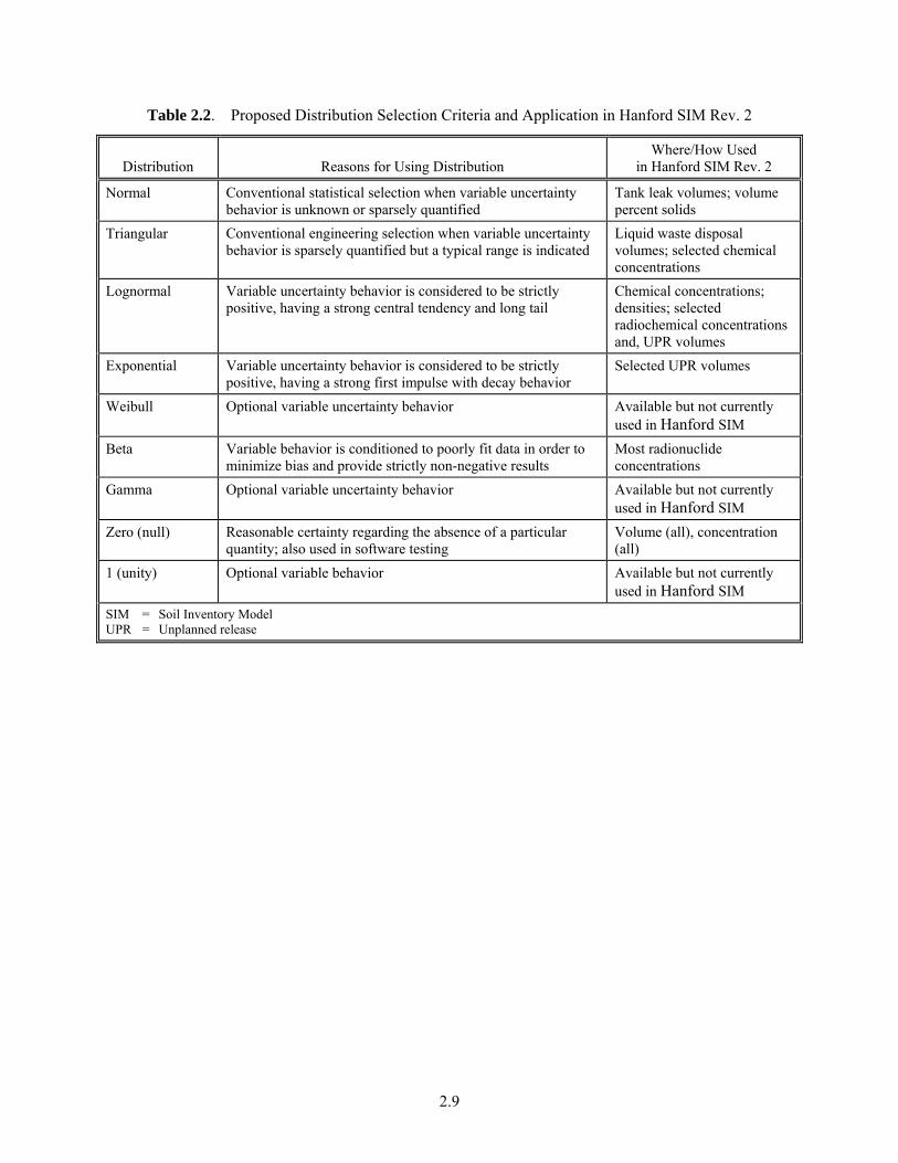
Table 2.2. Proposed Distribution Selection Criteria and Application in Hanford SIM Rev. 2

Distribution Reasons for Using Distribution Where/How Used

in Hanford SIM Rev. 2

Normal Conventional statistical selection when variable uncertainty behavior is unknown or sparsely quantified

Tank leak volumes; volume percent solids

Triangular Conventional engineering selection when variable uncertainty behavior is sparsely quantified but a typical range is indicated

Liquid waste disposal volumes; selected chemical concentrations

Lognormal Variable uncertainty behavior is considered to be strictly positive, having a strong central tendency and long tail

Chemical concentrations; densities; selected radiochemical concentrations and, UPR volumes

Exponential Variable uncertainty behavior is considered to be strictly positive, having a strong first impulse with decay behavior

Selected UPR volumes

Weibull Optional variable uncertainty behavior Available but not currently used in Hanford SIM

Beta Variable behavior is conditioned to poorly fit data in order to minimize bias and provide strictly non-negative results

Most radionuclide concentrations

Gamma Optional variable uncertainty behavior Available but not currently used in Hanford SIM

Zero (null) Reasonable certainty regarding the absence of a particular quantity; also used in software testing

Volume (all), concentration (all)

1 (unity) Optional variable behavior Available but not currently used in Hanford SIM

SIM = Soil Inventory Model UPR = Unplanned release

2.9

2.10

Table 2.3. Hanford SIM Rev. 2 Continuous Distributions

Distribution Technical Summary

The beta distribution is a very flexible distribution commonly used to represent variability over a fixed range. It can represent uncertainty in the probability of occurrence of an event. It is used also to describe empirical data and predict the random behavior of percentages and fractions (Decisioneering 2007, p. 274).

The exponential distribution is widely used to describe events recurring at random points in time or space, such as the time between failures of electronic equipment, the time between arrivals at a service booth, or repairs needed on a certain stretch of highway. It is related to the Poisson distribution, which describes the number of occurrences of an event in a given interval of time or space (Decisioneering 2007, p. 278).

The gamma distribution applies to a wide range of physical quantities and is related to other distributions: lognormal, exponential, Pascal, Erlang, Poisson, and chi-squared. It is used in meteorological processes to represent pollutant concentrations and precipitation quantities. The gamma distribution is also used to measure the time between the occurrence of events when the event process is not completely random. Other applications of the gamma distribution include inventory control, economics theory, and insurance risk theory (Decisioneering 2007, p. 280).

The lognormal distribution is widely used in situations where values are positively skewed, for example in financial analysis for security valuation or in real estate for property valuation (Decisioneering 2007, p. 285).

The normal distribution is the most important distribution in probability theory because it describes many natural phenomena, such as people’s IQs or heights. Decision-makers can use the normal distribution to describe uncertain variables such as the inflation rate or the future price of gasoline (Decisioneering 2007, p. 290).

The triangular distribution describes a situation in which the minimum, maximum, and most likely values to occur are known. For example, the number of cars sold per week when past sales show the minimum, maximum, and usual number of cars sold could be used to describe the anticipated behavior (Decisioneering 2007, p. 294).

The Weibull distribution describes data resulting from life and fatigue tests. It is commonly used to describe failure time in reliability studies and the breaking strengths of materials in reliability and quality control tests. Weibull distributions also are used to represent various physical quantities, such as wind speed (Decisioneering 2007, p. 299)

For a greater understanding of each type of distribution and its definition, refer to the Crystal Ball User Manual installed as part of the software, available at http://www.crystalball.com.

3.0 Input Modification through the Microsoft Excel User Interface

As previously noted, a series of Microsoft Excel worksheets (SiteInput, AnalyteInput, DensityInput, CorrFactors, Legend, and Setup) was created in a workbook as a user interface and integrated into a comprehensive model input data file. The following sections describe the steps necessary to make changes or additions to the variable definitions. Sections 3.1 through 3.3 describe the entry or modification of waste site data. Sections 3.4 and 3.5 describe the entry or modification of waste stream compositions. Section 3.6 describes the entry of waste stream densities for solid and liquid phases. It is incumbent on the analyst to ensure that each waste stream composition is mass-balanced, charge-balanced, and isotopically consistent. Hanford SIM, Rev. 2 does not perform those functions.

3.1 Adding or Editing a Site for Inclusion in the Simulation 1. Select the Legend sheet from the source workbook (ex. SIMInput) file (refer to Figure 2.2).

2. Examine the list that extends from column F cell 2 (F2) down to see if the site to be added already exists in the model. Certain legacy locations were removed from the current list of sites but remain as potential selections in the model.

3. At the bottom of the list started in cell F2 (or in F2 if it is blank and a new series of sites is being simulated), enter the name of the site. There cannot be any blank spots in the list (e.g., the list must be continuous and sequential), and the site label must be unique. Copy and paste this label into the SiteInput sheet where it is needed.

4. In Column E, next to the name of the newly entered site, enter the next consecutive number. The number in column E should be the row into which the site was added minus 1. If the site was added into cell F527, the index value in E527 should be 526.

5. On the same row, in column D, enter the name of the operable unit (e.g., category) to which the site belongs. If this is an operable unit name that has been used before, it is recommended that the label be copied and pasted into this cell to ensure that the name is identical to the one used before.

6. If a site label needs to be edited, the name can be edited in the Legend sheet, and the previous label can be replaced in the SiteInput worksheet as a correction. Copy and paste this label into the SiteInput sheet where it is needed.

3.2 Adding or Editing Site Volumes

Quantifying and parameterizing the waste volume for a site involve a significant degree of analysis and judgment, the details of which are outside the scope of this user’s guide. However, as a brief over-view of this process, the initial step in this phase is identifying and verifying source information and assumptions regarding the site’s overall volume, individual volume contributions, and operating life (e.g., annual waste receipts).

This information must then be entered into the SiteInput worksheet in the appropriate cells, must be in a form that can be used by the program (e.g., properly assigning and quantifying the distributions), and must not violate any of the various physical, chemical, or mathematical boundary conditions inherent in the simulation (e.g., waste volumes are greater than or equal to 0, lognormal distributions are strictly

3.1

positive). The indices in the Legend #, s (Legend worksheet site index number) and Legend #, w (Legend worksheet waste stream index number) are assigned as part of simulation initialization and are not part of the data entry in the SiteInput worksheet.

The default total volume unit basis is megaliters (e.g., in the SiteInput file, a value of 1 = 1,000,000 L); the volume percent solids basis is percent, expressed as a decimal (e.g., in the SiteInput worksheet, a value of 0.01 = 1%). Table 3.1 illustrates an example of the Hanford SIM data structure for site-date-volume description. The data input process for completing an entry in the SiteInput worksheet follows:

1. From the source workbook file, select the SiteInput sheet.

2. Enter the site label, corresponding to the site name in the Legend worksheet (copy-paste is recommended).

3. Enter the site year of operation for that waste site–waste stream–year combination (from 1944 to 2001).

4. Enter the site waste stream label, corresponding to the site name in the Legend worksheet. (copy-paste is recommended).

5. Enter the distribution type for the waste volume (refer to Table 2.1).

6. Enter the parameterization for total volume for that waste site–waste stream–year entry.

7. Enter the parameterization for volume percent solids for that waste site–waste stream–year entry.

8. Once entered, the quantitative description can be modified as needed. If revisions to the input definition are necessary as a result of newly discovered site information (or other technical/programmatic reasons), maintaining a change control log is recommended to provide traceability and defensibility of the rationale for the change.

Table 3.1. SiteInput Worksheet Example, Hanford SIM Rev. 2

Legend #

Legend #

Site Year Waste Stream

Dist Type

Total Volume (ML) Dist Type

Vol % Solids

s w Parm 1 Parm 2 Parm 3 Parm4 Parm 1 Parm 2 Parm 3 Parm 4

1 45 200-E-100 1945 BiPO4 (BT1) Cool Wtr-Stm Cond

1 0.00219 0.00438 0.00657 0 17 0 0 0 0

65 50 216-A-19 1955 PUREX (P1) Cold Start

1 0.825 1.10 1.38 0 1 0.045 0.09 0.125 0

3.3 Adding a Waste Stream Entry

There can be as many waste streams as required (within certain practical limits) to perform a simulation in Hanford SIM. The label identifying the waste stream must be defined in the Legend worksheet and is assigned by the analyst when defining the site in the SiteInput worksheet. The waste stream must also be assigned a unique and appropriately descriptive label. Although Hanford SIM does not use the waste stream and waste site location labels per se as part of the calculation, well-selected

3.2

waste site and waste stream labels assist in troubleshooting, analysis, and evaluation of the simulation inputs and outputs as well as providing traceability to reference documentation and data.

The waste stream must also be assigned an index number as part of a list of sequential integers in the Legend worksheet; the index number is assigned as part of the simulation initialization. Without an index number, the code will not execute and an error message will be generated.

1. From the source workbook, select the Legend worksheet (Figure 2.2).

2. At the bottom of the list in column M, enter the name of the new waste stream. Also, verify that this is a new waste stream and there is not an entry for this waste stream already.

3. In column N, next to the new waste stream name, enter in the index number for this line. This number should be one greater then the index number above it.

4. Define the composition of the waste stream and incorporate it into the AnalyteInput worksheet. This composition must be comprehensive and include a description for each analyte/radionuclide together with a definition of uncertainty. Additionally, analyte constituent lists for all waste streams must be identical.

3.4 Defining Analyte Concentrations in a New Waste Stream

The concentration unit bases are micrograms/gram for chemical constituents or microcuries/gram for radionuclides (radionuclides values in the AnalyteInput worksheet are inflated by 1E+09 from the reference document values to allow for very small values that are present in other waste streams and corrected later in the inventory calculation using the correction factors). Table 3.2 illustrates an example of the Hanford SIM data structure for waste stream-analyte descriptions. The data entry process for entering a new waste stream into the AnalyteInput worksheet follows.

1. From the source workbook file, select the Legend sheet.

2. Copy the analyte list from column I.

3. Select the AnalyteInput worksheet and paste the analyte list at the bottom of the list in column D.

4. Copy and paste the corresponding analyte index numbers from Column H of the Legend worksheet into the AnalyteInput worksheet in column B.

5. From the Legend worksheet, copy the label of the waste stream from Column M.

Table 3.2. AnalyteInput Worksheet Example, Hanford SIM Rev. 2

Legend #

Legend #

Waste Stream_

Unc Analyte Dist - liquid

Derivation Worksheet Liquids Input (µg/g or μCi/g; radionuclides *1.0E+9) Dist –

Solid

Derivation Worksheet Solids Input (μg/g or μCi/g; radionuclides *1.0E+9)

w A Parm 1 Parm 2 Parm 3 Parm 4 Parm 1 Parm 2 Parm 3 Parm 4

1 1 1C Evap (BT2) Na 4 8.99E+04 1.40E+04 3.43E+05 0 4 1.78E+05 2.77E+04 6.78E+05 0

1. Paste the waste stream label into column C for every row into which the analyte list was pasted.

2. Copy and paste the waste stream index number from the Legend worksheet column L into the AnalyteInput worksheet column A for each row into which the analyte label was pasted.

3.3

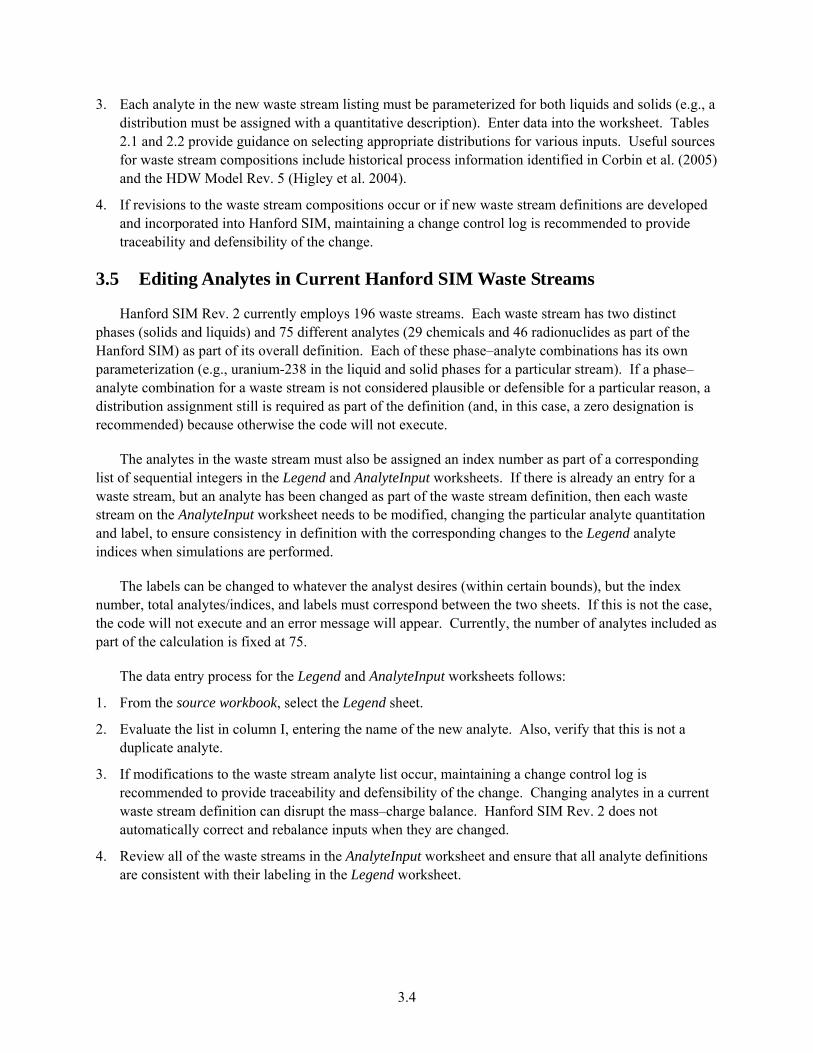
3. Each analyte in the new waste stream listing must be parameterized for both liquids and solids (e.g., a distribution must be assigned with a quantitative description). Enter data into the worksheet. Tables 2.1 and 2.2 provide guidance on selecting appropriate distributions for various inputs. Useful sources for waste stream compositions include historical process information identified in Corbin et al. (2005) and the HDW Model Rev. 5 (Higley et al. 2004).

4. If revisions to the waste stream compositions occur or if new waste stream definitions are developed and incorporated into Hanford SIM, maintaining a change control log is recommended to provide traceability and defensibility of the change.

3.5 Editing Analytes in Current Hanford SIM Waste Streams

Hanford SIM Rev. 2 currently employs 196 waste streams. Each waste stream has two distinct phases (solids and liquids) and 75 different analytes (29 chemicals and 46 radionuclides as part of the Hanford SIM) as part of its overall definition. Each of these phase–analyte combinations has its own parameterization (e.g., uranium-238 in the liquid and solid phases for a particular stream). If a phase–analyte combination for a waste stream is not considered plausible or defensible for a particular reason, a distribution assignment still is required as part of the definition (and, in this case, a zero designation is recommended) because otherwise the code will not execute.

The analytes in the waste stream must also be assigned an index number as part of a corresponding list of sequential integers in the Legend and AnalyteInput worksheets. If there is already an entry for a waste stream, but an analyte has been changed as part of the waste stream definition, then each waste stream on the AnalyteInput worksheet needs to be modified, changing the particular analyte quantitation and label, to ensure consistency in definition with the corresponding changes to the Legend analyte indices when simulations are performed.

The labels can be changed to whatever the analyst desires (within certain bounds), but the index number, total analytes/indices, and labels must correspond between the two sheets. If this is not the case, the code will not execute and an error message will appear. Currently, the number of analytes included as part of the calculation is fixed at 75.

The data entry process for the Legend and AnalyteInput worksheets follows:

1. From the source workbook, select the Legend sheet.

2. Evaluate the list in column I, entering the name of the new analyte. Also, verify that this is not a duplicate analyte.

3. If modifications to the waste stream analyte list occur, maintaining a change control log is recommended to provide traceability and defensibility of the change. Changing analytes in a current waste stream definition can disrupt the mass–charge balance. Hanford SIM Rev. 2 does not automatically correct and rebalance inputs when they are changed.

4. Review all of the waste streams in the AnalyteInput worksheet and ensure that all analyte definitions are consistent with their labeling in the Legend worksheet.

3.4

3.5

3.6 Adding a Waste Stream Density Definition

Each waste phase for each waste stream must have a density definition. This label must be identical between the Legend worksheet, SiteInput worksheet, and DensityInput worksheet. It must also be assigned the corresponding index number as part of a list of continuous, sequential integers in the Legend and DensityInput worksheets; the code will not execute otherwise.

The default density concentration unit bases are grams/milliliter for both phases. Table 3.3 is an example of the Hanford SIM data structure for waste stream–density descriptions. The data entry process for the DensityInput worksheet is as follows:

1. From the source workbook file, select the Legend worksheet.

2. Copy the waste stream label list and index list from columns L and M.

3. Select the DensityInput worksheet and paste the list into cell A3.

4. Define and parameterize each waste stream according to guidance in Table 3.3 using selected source data, such as the HDW Model Rev. 5, subject-matter expertise, or other historical process information.

Table 3.3. DensityInput Worksheet Example, Hanford SIM Rev. 2

Legend # Waste Streams—

Current

Supernatants Density (g/mL) Solids

Density (g/mL)

w Dist Type Parm

1 Parm

2 Parm

3 Parm

4 Dist Type

Parm 1

Parm 2

Parm 3

Parm 4

1 1C Evap (BT2) 4 1.26 0.063 0 4 1.77 0.088 0 0

3.7 Determining Correction Factor Values

The CorrFactors worksheet contains scalar values that are used to convert units of the analyte inventories calculated in SIM to those desired by users as input in their models. These values do not have uncertainties. The unit basis for the chemical analytes allows the correction factor to be 1 for results to be reported in kilograms.

The unit basis for radionuclides dictates that the correction factor be 1E-06 to provide for reporting results in curies, after correcting for the 1E+09 inflation factor applied to the radionuclide inputs. However, if the reporting requirements for Hanford SIM are changed and different units are desired, the correction factor values can be modified as needed. Figure 3.1 illustrates the inputs in the CorrFactors worksheet with the identifying analyte index number and label from the Legend and the values for each phase used in the calculation.

Figure 3.1. CorrFactors Worksheet Example

4.0 Executing a Soil Inventory Model Simulation

After a source workbook (ex. SIMInput) file is prepared with the desired sites, waste streams, compositions, and simulation parameters, the next step is to run Hanford SIM. Figure 4.1 illustrates a typical user flow for performing a simulation.

1. As a good practice, inspect and prepare the computers and files for use. Additionally, before simulation,

a. Use an uninterruptible power supply (UPS).

b. Run a COTS memory check such as Memtest86.

c. Disable virus and operating system scans/updates and isolate the computers from any network connections.

d. Configure and review input files for use.

2. Open the Hanford SIM dialog box by double-clicking on the OCBHanford shortcut.

3. Select File: Open. Select the prepared source workbook file and open it from the dialog box.

4. In Microsoft Excel, verify the simulation administration settings.

a. From the Setup sheet (in Figure 2.1):

i. There must be 21 percentiles entered. Each percentile must be unique and in descending order.

ii. The number of trials must be entered. The number of trials necessary for a converged simulation is not usually known a priori. Testing to determine model stability is described in Section 5.1; however, for general troubleshooting, much smaller values such as 100 or 1,000 trials can be used to conserve time before running a complete simulation.

iii. Sampling method must be selected (0 for Monte Carlo, 1 for LHS).

iv. If LHS is selected, fill in the sample size. This number must be an integer, and the result of the ratio of trials to sample size must result in an integer. It is strongly recommended that values for this parameter be less then or equal to 1/50th of the number of trials. For example, if the number of trials is 25,000, then the sample size should be 500.

v. Trials per loop must be an integer evenly divisible into the number of trials and no greater than the number of trials. Otherwise, the total number of trials selected will not be run. Larger values for this parameter improve performance but also risk exceeding the memory available on the machine, causing the simulation to fail. For example, if the number of trials is 25,000, then a potential value for this parameter is 2,500, providing 10 calculational loops for completing a simulation. New input distributions are created as a function of the number of calculational loops, minimizing a potential source of bias.

vi. Save Directory. This directory is where the final results of this simulation are stored, including the updated source workbook file.

4.1

4.2

Figure 4.1. Hanford SIM Rev. 2 User Flow Diagram

b. From the Legend sheet (in Figures 2.2 and 2.3):

i. Operable Units (Column R). “Operable Units” is a label used to define a category of waste sites considered to be related in Hanford SIM Rev. 2. This term and grouping label could be used for any collection of sites the user deems interesting or appropriate. In addition, sometimes performing a simulation with some operable units (OUs) removed is desirable. To do this, place an “x” in column R next to the operable unit name that does not need to be run. Verify that each OU desired to produce results has a blank in column R next to its name and press the Remove Selected Operable Units button.

ii. Split. If using the distributed computing function, pressing the Update Operable Unit List and Split into Sections button after parameterizing the input file as directed in Section 3.1.1 will configure a sub-file for simulation as directed in Section 4.1.1.

iii. Sites (Column C). Sometimes performing a simulation with some sites removed is desirable. To do this, place an “x” next to the site name in column C.

iv. Analytes (Column G). Sometimes performing a simulation with some analytes removed is desirable. To do this, place an “x” next to the analyte name in Column G. This function does not affect the input composition definition of the waste stream; it simply removes the analyte from the calculation and output.

5. The source workbook file can then be checked for inconsistencies or errors by checking the appropriate box and selecting “Test Distributions” [see Figure 2.4(a)]. Place a check next to Check Distribution Parameters Only (No Calc). During initialization of the model, several actions occur. The site labels in the SiteInput spreadsheet are matched to the site labels in the Legend spreadsheet and indexed to their specific site identification numbers from the Legend spreadsheet. These indices are assigned to the first column of the SiteInput sheet and are used by the OCB interface to execute and administer the calculation. Similarly, the waste stream labels in the SiteInput spreadsheet are matched to the waste streams in the Legend spreadsheet and indexed to their specific waste stream identification number from the Legend spreadsheet and assigned the waste stream identification numbers to the second column of the SiteInput sheet.

6. Click the Test Distributions button (note the Test Distribution button will appear in place of the Calculate button in Figure 2.4(a) when the Check Distribution Parameters Only box is checked). The program will verify that the model input parameters pass a few basic tests. The code will then review the various input definitions and assign the index identification numbers used to organize the inputs and calculate the results.

a. If there is an “Initialization Successful” message, uncheck the Check Distribution Parameters Only (No Calc) and move on to step 7.

b. If there is an error, note the error message(s) for information as to where the errors are and what type of problem was encountered. Correct them and save the corrected file for simulation. In certain cases, an error may not manifest until the calculation commences or, if the user has disregarded the warning dialogs, the execution will encounter the latent error. If a simulation is activated without correction or with a latent error, an error log will be generated. Check the error log for a comprehensive description of the errors present, make the necessary corrections, and save the corrected file for re-simulation.

7. Now the model is ready to be run. Once the model is initialized, unchecking the Check Distribution Parameters Only (No Calc) box and selecting Calculate will activate Hanford SIM and calculation

4.3

will commence. If during simulation a problem is discovered or if the user has a need, there are Pause and Cancel commands that will alternately temporarily suspend the simulation or stop and quit the application entirely as desired. Hanford SIM may require anywhere from several minutes to multiple weeks to complete, depending on settings.

4.1 Distributed Computing

For complex simulations with large numbers of site-year inputs, it is desirable in the interest of time to run the model across multiple computers, each processing a specific portion of the inputs and reconstituting the full set of simulation results post-process.

4.1.1 Splitting Runs

After preparing a source workbook (ex. SIMInput) file for simulation,

1. Place a copy of the source workbook file onto each computer that will be used.

2. Repeat these steps on each computer:

a. Open the source workbook file.

b. Select the Legend sheet (see Figure 2.3).

c. In cell X21, enter how many computers will be used, up to 10.

d. In cell X22, designate a number for this computer in the group to be used. (If this computer is the first of four computers used, then enter “1.” If it is the second of four computers used, enter “2,” and so on.)

e. Press the Update Operable Unit List and Split into Sections button. Wait for the macro to run and process the file.

f. Save the file with an informative label and close the split source workbook (ex. SIMInput_1, SIMInput_2, etc.). This action will create the various sub-files that will be individually simulated.

g. Do the same for each computer to be used, until the source file has been completely subdivided.

3. Perform the seven steps in Section 4, Executing a Soil Inventory Model Simulationl, ensuring that all of the run settings are identical for each computer being used (i.e., number of trials, seed, Monte Carlo or LHS, and other settings).

4.1.2 Merging the Runs

Because of the size and run times associated with Hanford SIM, a simple distributed computing function was incorporated. The distributed computing management function was placed in the Legend worksheet of the production workbook. By placing an "X" or "x" in the appropriate column then executing the macro OpUnit_Selection, the corresponding sites of that operable unit are removed from the simulation. By using the Update Operable Unit List and Split into Sections macro command, the computer automatically loads a file that is reasonably balanced as a function of the number of machines used to perform a simulation with the pieces having approximately concurrent run-time completions.

These pieces are estimated using the number of site-year elements as a metric and are split into roughly equal numbers. However, sites within a specified operable unit are conserved (i.e., all members

4.4

4.5

of an operable unit grouping are maintained together) within the same sub-file. A simulation can be split among as many as 10 machines.

Each computer used for a distributed run will have a portion of the results. Each of those output sections must be merged together to make a useable and complete set of results. The reconstitution macro, activated by the button Merge Summaries, begins execution at the top of the list and works its way down. The code uses the Legend sheet within the listed source workbook (ex. SIMInput_1) files to determine which operable units/closure zones were simulated and, therefore, the files to be merged to the newly specified directory.

1. Copy the results of the sub-file from each computer used onto a single computer. Each portion needs to be in a separate folder. The folders should be named in such a way that the individual results can be traced back to the computer that executed that portion of the simulation.

2. Create a new folder. Clearly name the folder in such a way to indicate that this will be the merged results folder.

3. Copy one of the source workbook (ex. SIMInput) files from the partial result folders to the new merge folder. Append the name of the source workbook file with the word “merge” to note that this is the source workbook (ex. SIMInput_merge) that will contain all of the results when the merging is finished. (For example, if the source file being used is SIMInput_1000.xls, rename it SIMInput_1000_Merge.xls.)

4. Open the source workbook file, which was just renamed, from the merge directory.

5. Select the Legend sheet.

a. Clear any cells marked with an “x” in columns C, G, and R.

6. Select the Setup sheet.

a. In cells B39 through B48, enter the path for each partial result directory and the source workbook (ex. SIMInput) file in each of those folders. This path/filename must include the “.xls” extension at the end of the source workbook (ex. SIMInput) file name.

b. Press the Merge Summaries button. Verify that the macro is ready to run when the dialog boxes appear. Wait for the macro to finish executing.

c. If an error message appears at this point, verify the directory paths to each partial result, ensuring that the source workbook file that is currently open has had its name appended and is from the new merge folder. Clear the merge folder except for the source workbook file that is open, fix any error(s), and run the macro again.

7. Save and close the open source workbook file that was appended with the word “merge.” This source workbook is now the file of record for this set of results.

5.0 Quality Assurance and Error Recovery Guidance

Several different macro testing codes are used to evaluate the performance of the simulation and to confirm that Hanford SIM executed correctly. These codes test the stability of the Monte Carlo calculation (Convergence), run a test calculation on a selected site-analyte combination (Evaluate Top 10 List), run a series of separate qualifying calculations for convergence and arithmetic performance on a variety of different sites with different parameters (Blackboxtest_1), examine the waste volumes associated with a series of years or waste streams (VolumeBalance), and evaluate the model results with documented reference values at various levels of resolution (cCDIcompare and Zero_0_1_Compare).

5.1 Convergence

Convergence testing ensures repeatability and stability of the model operation and the results produced. Development of convergence criteria is user-defined. The results for Hanford SIM include evaluations at the 5% and 10% deviation rate for the selected percentiles/outcomes (mean, median, standard deviation, 0.5th percentile, 5th percentile, 95th percentile, and 99.5th percentile). Corbin et al. (2005) discuss and illustrate the convergence testing protocol that was used. Perform the following steps to complete convergence testing:

1. Create a new folder and place a copy of the convergence testing Excel file into the new directory.

2. Open the convergence file (Convergence; see Figure 5.1).

3. Open the source workbook used to generate results.

4. Select the Legend sheet. Select the list of the operable units (in cells Q2 to the bottom of that list), and copy them.

5. Using the open copy of the convergence file; paste the operable unit list into cell B8.

6. Close the source workbook file. (Do not save.)

7. Specify the directory path for each result set in cells B1 through B5. The end of the directory path must end with the “\”. At least two directories must be specified, and up to five sets of results can be used. Using five different sets of results is recommended to verify repeatability.

8. Press the Run Convergence button and wait for the macro to finish. This action can take several hours.

9. The results from this test are reported in columns F through M of the Convergence worksheet file (see Figure 5.2).

10. The corrected convergence values for identified/specified small number errors at the 0.5th and 5th percentile are listed in cells J60 to J62 and K60 to K62.

5.1

Figure 5.1. Convergence User Interface

5.2

Figure 5.2. Convergence Test Output

5.3

When the convergence macro is completed, ensure that each “drop” line on the graph produced approximately aligns with other lines. If one of the “drop” lines behaves substantially differently than the others (if that “drop” is much lower then the others and is by itself), then note which run was removed from that comparison and track that run to the computer used.

That type of quantitative behavior from the test indicates either 1) potential hardware errors were introduced in the simulation, or 2) a potential outlier was generated. In either case, a new simulation should be run as part of the final results file, potentially on a different machine. If there is an interest in the results of a specific operable unit, each operable unit has a file created that contains the entire individual site comparisons run for that operable unit.

5.2 Top 10 Lists

This tool uses the three Top 10 lists for each analyte for a specific simulation as a basis for evalu-ation. The first list is determined by the highest mean inventory (Column A through Column H). The second is determined by the greatest median inventory (Column I throughColumn P). The third list consists of the sites with the highest relative standard deviation (Column Q through Column X).

The SiteEval (Site Evaluation) spreadsheet is a diagnostic tool output that allows investigation of a specific analyte inventory at a specific site in the Top 10 list. Selecting the site name from a list and pressing the Evaluate Top 10 List button at the top of the page runs a Crystal Ball simulation for that one analyte for that site for all years during which the site received waste.

On activation of the Evaluate Top 10 List macro, the SiteEval worksheet will be populated with the model input parameters and uncertainty definitions for that site–analyte combination and will run a conventional Crystal Ball Monte Carlo scenario so that the individual contributing elements to the total inventory can be evaluated. However, the SiteEval spreadsheet can run only one site–analyte combination at a time on the Top 10 list, although multiple evaluation scenarios could be saved in a separate workbook if the user so desires.

Inputs to the calculation and the results will be shown on the SiteEval sheet of the source workbook file. Columns AY6 through BE(x); where x is the number of waste stream-years contain the Crystal Ball results for each waste stream and year contribution to the site total. The area formatted with a light yellow background at the bottom of the Crystal Ball simulation in columns AY through BF contain the results from the OCB-based Hanford SIM run for comparison purposes.

5.3 Blackbox Test

This test verifies that the results for sites with the 10 highest relative standard deviations for each analyte and their associated median values are calculated the same by Crystal Ball and by OCB. The Test_BlackBox1 macro command performs an independent test of the OCB results by running the Top 10 list outputs for the relative standard deviation results comprehensively through the Evaluate Top 10 List macro and compares those results to the output obtained using regular Crystal Ball. The results are reported to the BlackBoxTest1 sheet. This test is done as an internal QA consistency check to establish that the model parameters and computation commands are functioning correctly, the calculations are being performed correctly, and as a second check on whether the convergence criteria are being satisfied.

5.4

This test serves as a double check for the validity of the OCB results by verifying the outcomes of the calculations using a different piece of software and evaluating the results to ensure that they are within the user-defined quality assurance tolerances. If the Crystal Ball-based outcomes for relative standard deviation or median are substantially different for any of the site–analyte combinations, then that result is counted as an error. As a result of the intrinsic modeling variability of these sites and the associated possible small number errors, perfect agreement between the OCB and Crystal Ball is not expected. Error rates will vary depending on parameterizations used in the model and the error tolerance defined as part of this test.

1. Open the source workbook file located in the results directory.

2. Press Alt-F8 to bring up the run macro dialog box. (This can be done also through Tools menu→Macro → Macros.)

3. Select Test_Blackbox1, and press run.

4. This process will take approximately 4 hours for the Hanford simulation (Corbin et al. 2005) to complete on a computer with the recommended hardware and software configuration with the same simulation parameterizations. The results will be reported in columns A-H.

5. When completed, select the BlackBoxTest1 sheet.

a. The number of results that fall out of the specified tolerance for relative standard deviations and medians (in this case, 5%) is found in cells M10 and N10 respectively.

b. The error rate percentage for relative standard deviation and median are listed M11 and N11, respectively.

5.4 Volume Balance Macro

The volume balance macro is a diagnostic tool that allows for the checking of volumes used in the SiteInput. It provides a compact way of reviewing the total volumes of waste discharged in three ways: by waste stream as a function of time; by year, with each total waste stream contribution; and by total waste stream volume. Thus, waste losses can be reconciled and allocated to the proper time and amount. This worksheet aids in enforcing the overall mass balance boundary condition and can assist in evaluating analyte solubilities and volume percent solids lost.

1. Beginning with an open source workbook, press Alt-F8 to bring up the macro selection window (or access via the Tools menu → Macro → Macros).

2. Select volume balance from the list of macros and press the run button. Wait briefly for the macro to finish executing.

3. Results will be written to the VolumeBalance sheet in the source workbook file.

This macro provides three sets of results. The first set of columns (A through C) shows the total volume of each waste stream discharged by year. The next set of columns (E through G) shows the total volumes discharged each year of the model as a function of waste stream. The last set of columns (I through K) displays the sum of the total volume mean values used for each waste stream, providing a comprehensive volume discharge estimate.

5.5

5.5 Other Quality Assurance and Error Recovery Tests

A variety of macro commands assemble specific sets of Hanford SIM results to compare to reference values at differing levels of resolution. The results of these comparisons are then written to the appropriate worksheets within the source workbook file. The principal evaluation command is cCDIcompare.

1. Open the current source workbook file.

2. Navigate to the most current series of operable unit workbook files.

3. Select the operable unit workbooks that have comparable reference data and open them.

200-W Ponds Zone, Purex Zone PFP Zone 200-E Ponds Zone T Farm Zone U Plant Zone Semi-Works Zone B Farm Zone WTP-ETF-A-C Farm Zone S-U Farm Zone REDOX Zone B Plant Zone WM Zone T Plant Zone NRDWL-BC Control Zone Solid Waste Zone

4. Press Alt-F8 to bring up the macro selection window (or access via the Tools menu -> Macro -> Macros).

5. Select cCDIcompare from the list of macros and press the run button. Wait briefly for the macro to finish executing.

6. Results will be written to the cCDIDatabaseQuery, the individual cCDI analyte comparison sheets (Pu239, U238, Cs137, and Sr90), and the 0,1,2 compare in the source workbook file and comparison metrics developed.

The cCDIcompare macro will populate the specified cells in the various worksheets for evaluation, and the results of the comparisons are tabulated and reported. The 0,1,2 compare worksheet provides global and rolled-up high-level comparisons with regard to the site categories. The specific analyte comparisons for plutonium-239, uranium-238, cesium-137. and strontium-90 worksheets have the resulting simulation percentile values and the comparisons reported in them. These results are consolidated also in the cCDIDatabaseQuery worksheet using the lessthan worksheet as part of the comparison process.

5.6

5.7

The Zero_0_1_compare macro command has other subroutines that execute when this global macro is activated (insertlessthansfor_blues, and insertlessthansfor_bluesandgreens). It writes the results to the 0,1,2 compare worksheet. Zero_0_1_compare must be activated after cCDIcompare. These subsequent commands can be executed individually, through the Tools menu, but are usually done as part of the overall comparison testing.

Subroutines (insertlessthansfor_blues, and insertlessthansfor_bluesandgreens) in the macro modify the comparison metrics appropriately so as not to penalize the model performance. Additionally, the comparisons require a one-to-one correspondence for the comparisons to be valid. Thus, a site that does not have an inventory estimate from Diediker (1999) for one of the analytes is excluded from this evaluation and any further quantitative comparisons. Cells colored blue are the “less than” values included in Diediker (1999); cells colored light green are the “less than” values found in other source documents that were not carried forward as “less than” values. Other cells, shaded yellow, highlight corrections to the supplied data that were incorporated as part of this comparison. These corrections have been incorporated and documented as part of Table 6-32 in Section 6 of Corbin et al. (2005).

The simulation results for a site are compared with the information from specific reference data, and the number of reference data values Diediker (1999) that fall within the 99th percentile range are counted as agreement. Simulation results that disagree with the reference data are counted and qualified as out-of-range either high or low.

6.0 Hanford SIM Rev. 2 Outputs

The results generated by Hanford SIM Rev. 2 are written to the results folder specified in the Setup worksheet, with the number of individual workbooks dictated by the Legend worksheet. There are two places Hanford SIM-created outputs can be found depending on the level of resolution needed. The individual category (operable unit) workbooks in the Results folder have the comprehensive results for each site–analyte–year result, and the source workbook file has a variety of summary-level results compiled in various worksheets (Top 10 List; SumFrcLiq, SumFrcSol; SumFrcTot). Other outputs are generated as a result of executing macro commands after Hanford SIM has completed execution (e.g., the System Assessment Capability model output).

6.1 Category (Operable Unit) Workbook Results

The comprehensive Hanford SIM outputs are reported in separate workbooks organized by category as specified by the user. In the case of the Hanford simulation, the selected category designation was operable unit. They are created and populated automatically by OCBHanford in the folder designated in the Setup worksheet, with multiple model runs of the same input file assigned separate folders (Results001, Results002, and so on). The site grouping organization in the Legend can be constructed using any number of desired criteria; however, care must be taken to ensure that no output file exceeds the maximum length of a Microsoft Office 2003 Excel worksheet (65,536 rows). Otherwise, the computation will cause the computer to stall, and the code will not run to completion.

Each site–year–analyte–phase combination inventory result is reported along with total inventory results for each analyte by site and the comprehensive total for the operable unit. In addition, the input volume is described in terms of percentiles in order to derive a corresponding concentration percentile value for the site–year–analyte combination. Therefore, these concentration and volume percentile data are also calculated and are provided in the individual operable unit/closure zone results workbooks. Examples of these files can be found in Appendix C of Corbin et al. (2005).

6.2 System Assessment Capability Model Output Files

The category workbook outputs and consolidated results are useful in a variety of ways, from diagnosing systemic errors in modeling to evaluating specific site–year–analyte results of interest. However, the Inventory Module used in the System Assessment Capability (SAC) model (Bryce et al. 2002; Kincaid et al. 2006) to evaluate groundwater contamination requires the Hanford SIM-generated inventories to be decoupled into concentration and volume components to be used as inputs. These components are generated concurrently and reported together with the inventories providing a comprehensive, consolidated quantitative description of the site–year–analyte inventories, waste stream volumes, and aggregate waste compositions.

The previously described operable unit workbooks created by OCB cannot be used directly by the SAC model. For this reason, reformatting the results is required to make them usable by the SAC model. The Create SAC Output macro takes the specified set of output files in a directory and assembles them into a structure that can be read directly by the SAC model.

6.1

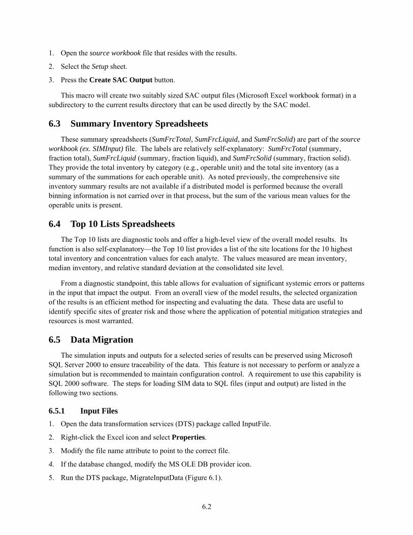
1. Open the source workbook file that resides with the results.

2. Select the Setup sheet.

3. Press the Create SAC Output button.

This macro will create two suitably sized SAC output files (Microsoft Excel workbook format) in a subdirectory to the current results directory that can be used directly by the SAC model.

6.3 Summary Inventory Spreadsheets These summary spreadsheets (SumFrcTotal, SumFrcLiquid, and SumFrcSolid) are part of the source

workbook (ex. SIMInput) file. The labels are relatively self-explanatory: SumFrcTotal (summary, fraction total), SumFrcLiquid (summary, fraction liquid), and SumFrcSolid (summary, fraction solid). They provide the total inventory by category (e.g., operable unit) and the total site inventory (as a summary of the summations for each operable unit). As noted previously, the comprehensive site inventory summary results are not available if a distributed model is performed because the overall binning information is not carried over in that process, but the sum of the various mean values for the operable units is present.

6.4 Top 10 Lists Spreadsheets The Top 10 lists are diagnostic tools and offer a high-level view of the overall model results. Its

function is also self-explanatory—the Top 10 list provides a list of the site locations for the 10 highest total inventory and concentration values for each analyte. The values measured are mean inventory, median inventory, and relative standard deviation at the consolidated site level.

From a diagnostic standpoint, this table allows for evaluation of significant systemic errors or patterns in the input that impact the output. From an overall view of the model results, the selected organization of the results is an efficient method for inspecting and evaluating the data. These data are useful to identify specific sites of greater risk and those where the application of potential mitigation strategies and resources is most warranted.

6.5 Data Migration The simulation inputs and outputs for a selected series of results can be preserved using Microsoft

SQL Server 2000 to ensure traceability of the data. This feature is not necessary to perform or analyze a simulation but is recommended to maintain configuration control. A requirement to use this capability is SQL 2000 software. The steps for loading SIM data to SQL files (input and output) are listed in the following two sections.

6.5.1 Input Files 1. Open the data transformation services (DTS) package called InputFile.

2. Right-click the Excel icon and select Properties.

3. Modify the file name attribute to point to the correct file.

4. If the database changed, modify the MS OLE DB provider icon.

5. Run the DTS package, MigrateInputData (Figure 6.1).

6.2

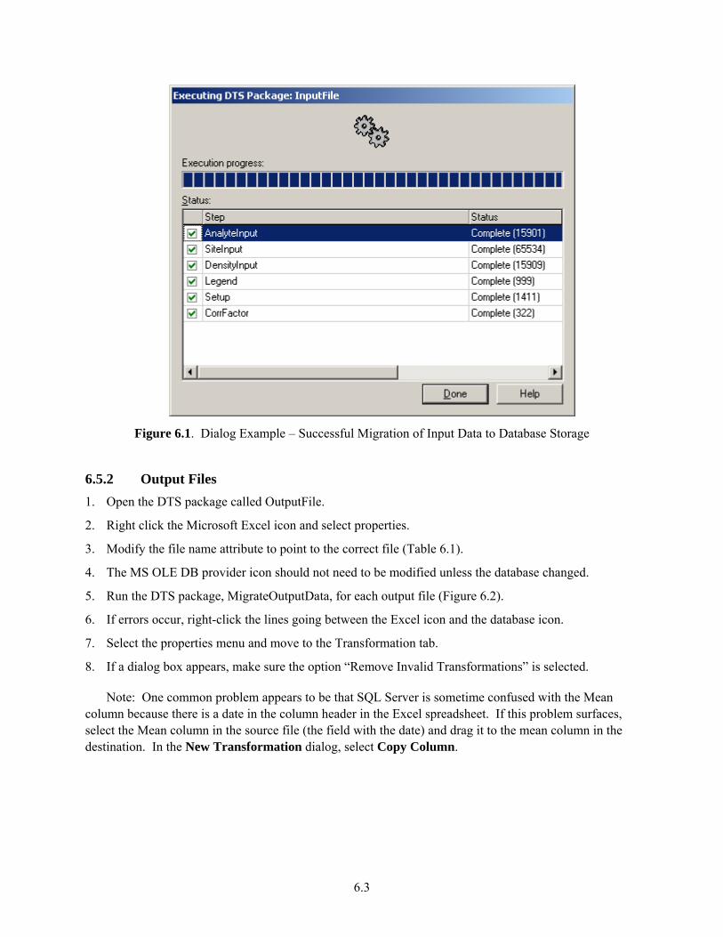
Figure 6.1. Dialog Example – Successful Migration of Input Data to Database Storage

6.5.2 Output Files 1. Open the DTS package called OutputFile.

2. Right click the Microsoft Excel icon and select properties.

3. Modify the file name attribute to point to the correct file (Table 6.1).

4. The MS OLE DB provider icon should not need to be modified unless the database changed.

5. Run the DTS package, MigrateOutputData, for each output file (Figure 6.2).

6. If errors occur, right-click the lines going between the Excel icon and the database icon.

7. Select the properties menu and move to the Transformation tab.

8. If a dialog box appears, make sure the option “Remove Invalid Transformations” is selected.

Note: One common problem appears to be that SQL Server is sometime confused with the Mean column because there is a date in the column header in the Excel spreadsheet. If this problem surfaces, select the Mean column in the source file (the field with the date) and drag it to the mean column in the destination. In the New Transformation dialog, select Copy Column.

6.3

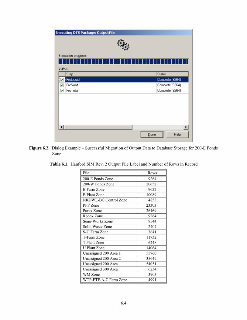
6.4

Figure 6.2. Dialog Example – Successful Migration of Output Data to Database Storage for 200-E Ponds

Zone

Table 6.1. Hanford SIM Rev. 2 Output File Label and Number of Rows in Record

File Rows 200-E Ponds Zone 9264 200-W Ponds Zone 20652 B Farm Zone 9622 B Plant Zone 10089 NRDWL-BC Control Zone 4853 PFP Zone 23303 Purex Zone 26169 Redox Zone 9264 Semi-Works Zone 9544 Solid Waste Zone 2407 S-U Farm Zone 3641 T-Farm Zone 11732 T Plant Zone 6248 U Plant Zone 14064 Unassigned 200 Area 1 55760 Unassigned 200 Area 2 35649 Unassigned 200 Area 54051 Unassigned 300 Area 6234 WM Zone 3903 WTP-ETF-A-C Farm Zone 4991

7.0 References

Agnew SF, J Boyer, RA Corbin, TB Duran, JR FitzPatrick, KA Jurgensen, TP Ortiz, and BL Young. 1997. Hanford Tank Chemical and Radionuclide Inventories: HDW Model Rev. 4. LA-UR-96-3860, Los Alamos National Laboratory, Los Alamos, New Mexico.

Anderson, MJ, Simpson BC, RA Corbin, and CT Kincaid. 2007. Hanford Soil Inventory Model (SIM) Rev. 2 Software Documentation Requirements, Design, and Limitations. PNNL-16940, Pacific Northwest National Laboratory, Richland, Washington.

Bryce RW, CT Kincaid, PW Eslinger, and LF Morasch (eds). 2002. An Initial Assessment of Hanford Impact Performed with the System Assessment Capability. PNNL-14027, Pacific Northwest National Laboratory, Richland, Washington.

Corbin RA, BC Simpson, MJ Anderson, WF Danielson, JG Field, TE Jones, and CT Kincaid. 2005. Hanford Soil Inventory Model, Revision 1. RPP-26744, Rev. 0, CH2M HILL Hanford Group, Inc., Richland, Washington.

Diediker LP. 1999. Radionuclide Inventories of Liquid Waste Disposal Sites on the Hanford Site. HNF-1744, Fluor Daniel Hanford, Inc., Richland, Washington.

Decisioneering. 2007. Crystal Ball 7.2.2 Users Guide. Decisioneering, Inc., Denver, Colorado.

Field JG and TE Jones. 2005. Tank Farm Vadose Zone Contamination: Volume Estimates for Risk Assessments. RPP-23405, Rev. 1, CH2M HILL Hanford Group, Inc., Richland, Washington.

Higley BA, DE Place, RA Corbin, and BC Simpson. 2004. Hanford Defined Waste Model, Rev. 5. RPP-19822, Rev. 0, CH2M HILL Hanford Group, Inc., Richland, Washington.

Iman RL and WJ Conover. 1982. “A Distribution-Free Approach to Inducing Rank Correlations Among Input Variables.” Communications in Statistics B11(3):311-334.

Kincaid CT, PW Eslinger, RL Aaberg, TB Miley, IC Nelson, DL Strenge, and JC Evans. 2006. Inventory Data Package for Hanford Assessments. PNNL-15829, Pacific Northwest National Laboratory, Richland, Washington.

Simpson BC, RA Corbin, and SF Agnew. 2001. Hanford Soil Inventory Model. BHI-01496, Rev. 0, Bechtel Hanford Inc., Richland, Washington.

Simpson BC, RA Corbin, MJ Anderson, and CT Kincaid. 2006. Hanford Soil Inventory Model (SIM) Rev. 1 Software Documentation Requirements, Design, and Limitations. PNNL-16098, Pacific Northwest National Laboratory, Richland, Washington.

Simpson BC, RA Corbin, MJ Anderson, and CT Kincaid. 2006. Hanford Soil Inventory Model (SIM) Rev. 1 User’s Guide. PNNL-16099, Pacific Northwest National Laboratory, Richland, Washington.

Watrous RA, DW Wootan, and SF Finfrock. 2002. Activity of Fuel Batches Processed Through Hanford Separations Plants, 1944 Through 1989. RPP-13489, Rev. 0, CH2M HILL Hanford Group, Inc., Richland, Washington.

7.1

A Appendix

Software Environment Maintenance

A.1

Appendix

Software Environment Maintenance

During the life of the project, operating system, application, and security patches were distributed for the various software packages used. This appendix provides a listing of the patches incorporated.

Microsoft Windows XP Professional, Version 2002, Service Pack 2

• Security Update for Windows XP (KB913433) • Windows Media Player 10 • Hotfix for Windows XP (KB896344) • Update For Windows XP (KB894391) Installed On 8/29/2006 • Security Update For Windows XP (KB896358) Installed On 8/29/2006 • Security Update For Windows XP (KB896423) Installed On 8/29/2006 • Security Update For Windows XP (KB896424) Installed On 8/29/2006 • Security Update For Windows XP (KB896428) Installed On 8/29/2006 • Update For Windows XP (KB898461) Installed On 8/29/2006 • Security Update For Windows XP (KB899587) Installed On 8/29/2006 • Security Update For Windows XP (KB899589) Installed On 8/29/2006 • Security Update For Windows XP (KB899591) Installed On 8/29/2006 • Windows XP HotFix – (KB587333) Installed On 8/29/2006 • Security Update For Windows XP (KB890046) Installed On 8/29/2006 • Security Update For Windows XP (KB901214) Installed On 8/29/2006 • Security Update for Windows XP (KB902400) Installed On 8/29/2006 • Security Update For Windows XP (KB904706) Installed On 8/29/2006 • Windows XP HotFix (KB888583) Installed On 8/29/2006 • Security Update For Windows XP (KB905414) Installed On 8/29/2006 • Security Update For Windows XP (KB905749) Installed On 8/29/2006 • Security Update For Windows XP (KB908519) Installed On 8/29/2006 • Security Update For Windows XP (KB893756) Installed On 8/29/2006 • Update For Windows XP (KB910437) Installed On 8/29/2006 • Update for Windows XP (KB911280) Installed On 8/29/2006 • Security Update For Windows XP (KB911562) Installed On 8/29/2006 • Security Update For Windows Media Player (KB911564) Installed On 8/29/2006 • Security Update For Windows XP (KB911567) Installed On 8/29/2006 • Security Update For Windows XP (KB911927) Installed On 8/29/2006 • Security Update For Windows XP (KB912919) Installed On 8/29/2006 • Windows XP HotFix – (KB889178) Installed On 8/29/2006 • Security Update For Windows XP (KB913580) Installed On 8/29/2006 • Security Update for Windows XP (KB914388) Installed On 8/29/2006 • Security Update For Windows XP (KB914389) Installed On 8/29/2006

A.1

• Windows XP HotFix – (KB888583) Installed On 8/29/2006 • Update For Windows XP (KB916595) Installed On 8/29/2006 • Security Update For Windows XP (KB917159) Installed On 8/29/2006 • Security Update For Windows XP (KB917422) Installed On 8/29/2006 • Windows XP HotFix – (KB888618) Installed On 8/29/2006 • Security Update For Windows Media Player 9 (KB917734) Installed On 8/29/2006 • Security Update For Windows XP (KB917953) Installed On 8/29/2006 • Windows XP HotFix – (KB888747) Installed On 8/29/2006 • Security Update For Windows XP (KB918439) Installed On 8/29/2006 • Windows XP HotFix – (KB888830) Installed On 6/29/2006 • Update For Windows XP (KB908531) Installed On 8/29/2006 • Security Update for Windows XP (KB920214) Installed On 8/29/2006 • Windows XP Hotfix – (KB889085) Installed On 8/29/2006 • Security Update for Windows XP (KB920670) Installed On 8/29/2006 • Security Update for Windows XP (KB920683) Installed On 8/29/2006 • Windows Genuine Advantage Notifications (KB905474) Installed On 8/29/2006 • Windows Genuine Advantage Validation Tool (KB892130) Installed On 8/29/2006 • Security Update for Windows XP (KB921398) Installed On 8/29/2006 • Security Update for Windows XP (KB921883) Installed On 8/29/2006 • Security Update for Windows XP (KB922616) Installed On 8/29/2006 • Security Update for Windows XP (KB901017) Installed On 8/29/2006 • Security Update for Windows Media Player 10 (KB917734) Installed On 9/22/2006 • Security Update for Windows XP (KB923414) Installed On 10/19/2006 • Security Update for Windows XP (KB919007) Installed On 10/19/2006 • Security Update for Windows XP (KB920685) Installed On 10/19/2006 • Security Update for Windows XP (KB923191) Installed On 10/19/2006 • Security Update for Windows XP (KB922819) Installed On 10/19/2006 • Security Update for Windows XP (KB924191) Installed On 10/19/2006 • Update for Windows XP (KB931836) Installed On 3/12/2007 • Security Update for Windows XP (KB924667) Installed On 5/26/2007 • Security Update for Windows Media Player 6.4 (KB925398) Installed On 5/26/2007 • Update for Windows XP (KB900485) Installed On 5/26/2007 • Security Update for Windows XP (KB923980) Installed On 5/26/2007 • Security Update for Windows XP (KB925902) Installed On 5/26/2007 • Security Update for Windows XP (KB926255) Installed On 5/26/2007 • Security Update for Windows XP (KB923694) Installed On 5/26/2007 • Security Update for Windows XP (KB927779) Installed On 5/26/2007 • Security Update for Windows XP (KB927802) Installed On 5/26/2007 • Update for Windows XP (KB927891) Installed On 5/26/2007 • Security Update for Windows XP (KB928255) Installed On 5/26/2007 • Security Update for Windows XP (KB928843) Installed On 5/26/2007 • Update for Windows XP (KB922582) Installed On 5/26/2007 • Security Update for Windows XP (KB930 178) Installed On 5/26/2007 • Update for Windows XP (KB930916) Installed On 5/26/2007

A.2

A.3

• Security Update for Windows XP (KB931261) Installed On 5/26/2007 • Security Update for Windows XP (KB931784) Installed On 5/26/2007 • Security Update for Windows XP (KB924270) Installed On 5/26/2007 • Security Update for Windows XP (KB918118) Installed On 5/26/2007 • Security Update for Windows XP (KB923689) Installed On 5/26/2007 • Security Update for Windows XP (KB920213) Installed On 5/26/2007 • Security Update for Windows XP (KB926436) Installed On 5/26/2007 • Update for Windows XP (KB920872) Installed On 5/29/2007 • Update for Windows XP (KB925720) Installed On 5/29/2007 • Windows Imaging Component Installed On 5/29/2007 • Update for Windows XP (KB920342) Installed On 5/29/2007 • Update for Windows XP (KB904942) Installed On 5/29/2007 • Hotfix for Windows XP (KB914440) Installed On 5/29/2007 • Update for Windows XP (KB920342) Installed On 5/29/2007 • Update for Windows XP (KB904942) Installed On 5/29/2007 • Update for Windows XP (KB936357) Installed On 7/11/2007 • Update for Windows XP (KB925876) Installed On 5/29/2007 • Hotfix for Windows XP (KB914440) Installed On 5/29/2007 • Security Update for Windows XP (KB932168) Installed on 5/29/2007 • Security Update for Windows XP (KB935840) Installed on 6/13/2007 • Security Update for Windows XP (KB929123) Installed on 6/13/2007 • Security Update for Windows XP (KB935839) Installed on 6/13/2007

Microsoft.NET 1.1 provides the application environment. These are the updates used as part of the development and production environment.

• Microsoft .NET Framework 1.1 Hotfix (KB928366) • Microsoft .NET Framework 2.0 • Security Update for Microsoft .NET Framework 2.0 (KB928365)

Microsoft Excel 2003; user interface for data input/output and analysis as part of Microsoft Office Professional 2003 with updates used as part of the development and production environment.

• Update for Office 2003: LCCWIZ • Office 2003 Service Pack 2 • Security Update for Office 2003: RICHED20 • Security Update for Office 2003: MSXML5 • Update for Office 2003: OTKLOADR • Update for Office 2003: STLIST • Security Update for Office 2003: GPFILTIff • Security Update for Excel 2003: EXCEL • Security Update for Office 2003: MSO

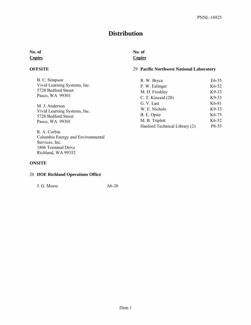
PNNL-16925

Distribution No. of No. of Copies Copies OFFSITE B. C. Simpson Vivid Learning Systems, Inc. 5728 Bedford Street Pasco, WA 99301 M. J. Anderson Vivid Learning Systems, Inc. 5728 Bedford Street Pasco, WA 99301 R. A. Corbin Columbia Energy and Environmental

Services, Inc. 1806 Terminal Drive Richland, WA 99352 ONSITE 20 DOE Richland Operations Office J. G. Morse A6-38

29 Pacific Northwest National Laboratory R. W. Bryce E6-35 P. W. Eslinger K6-52 M. D. Freshley K9-33 C. T. Kincaid (20) K9-33 G. V. Last K6-81 W. E. Nichols K9-33 B. E. Opitz K6-75 M. B. Triplett K6-52 Hanford Technical Library (2) P8-55

Distr.1