Hands-on Lab: LabVIEW – Charts, Graphs and Files Concept 1 ...€¦ · LabVIEW – Charts, Graphs...

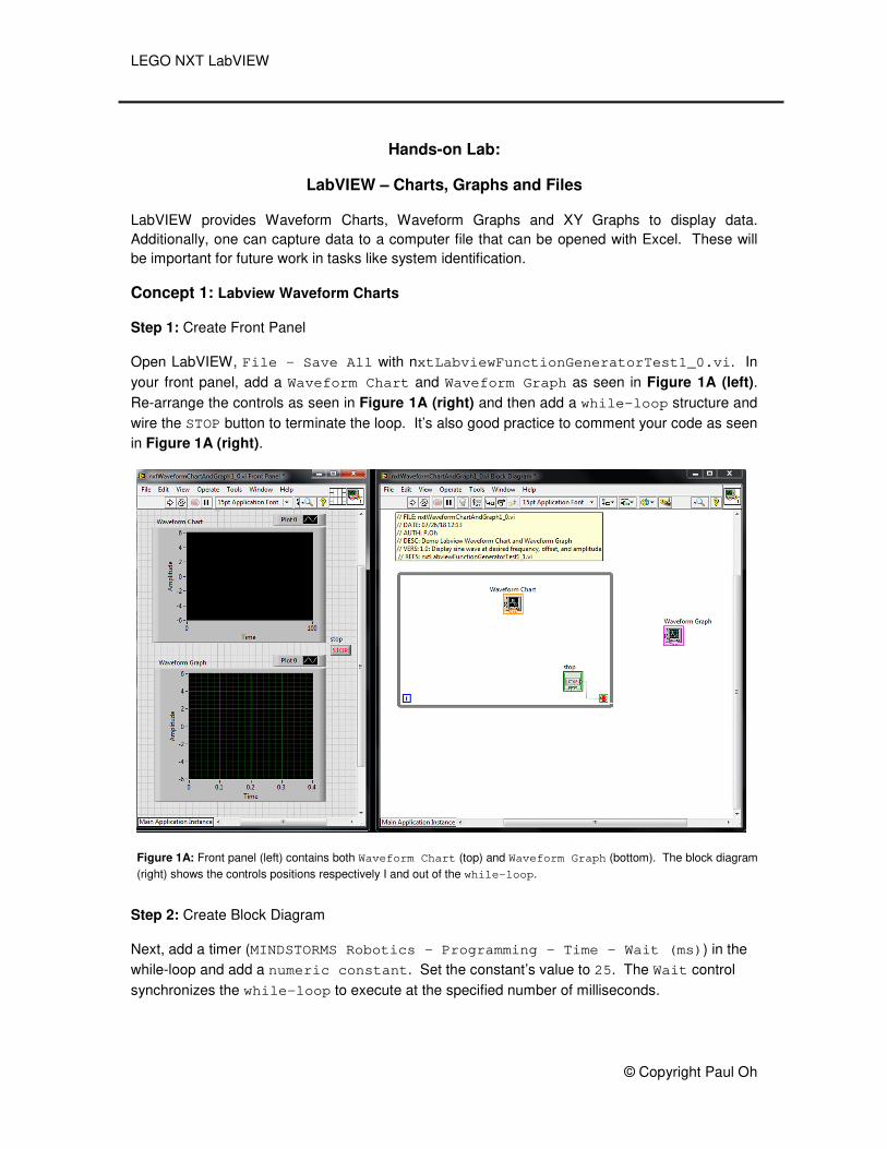
LEGO NXT LabVIEW

© Copyright Paul Oh

Hands-on Lab:

LabVIEW – Charts, Graphs and Files

LabVIEW provides Waveform Charts, Waveform Graphs and XY Graphs to display data.

Additionally, one can capture data to a computer file that can be opened with Excel. These will

be important for future work in tasks like system identification.

Concept 1: Labview Waveform Charts

Step 1: Create Front Panel

Open LabVIEW, File – Save All with nxtLabviewFunctionGeneratorTest1_0.vi. In

your front panel, add a Waveform Chart and Waveform Graph as seen in Figure 1A (left).

Re-arrange the controls as seen in Figure 1A (right) and then add a while-loop structure and

wire the STOP button to terminate the loop. It’s also good practice to comment your code as seen

in Figure 1A (right).

Step 2: Create Block Diagram

Next, add a timer (MINDSTORMS Robotics – Programming – Time – Wait (ms)) in the

while-loop and add a numeric constant. Set the constant’s value to 25. The Wait control

synchronizes the while-loop to execute at the specified number of milliseconds.

Figure 1A: Front panel (left) contains both Waveform Chart (top) and Waveform Graph (bottom). The block diagram

(right) shows the controls positions respectively I and out of the while-loop.

LEGO NXT LabVIEW


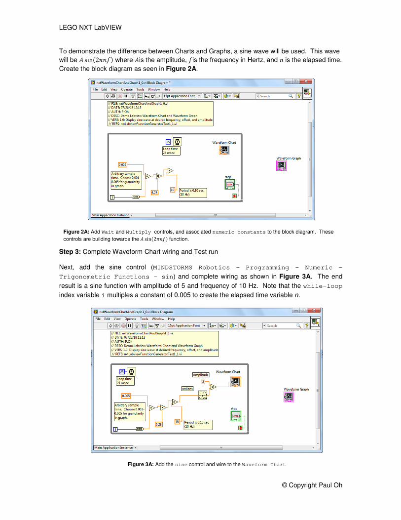
To demonstrate the difference between Charts and Graphs, a sine wave will be used. This wave

will be � sin�2�� where �is the amplitude, is the frequency in Hertz, and � is the elapsed time.

Create the block diagram as seen in Figure 2A.

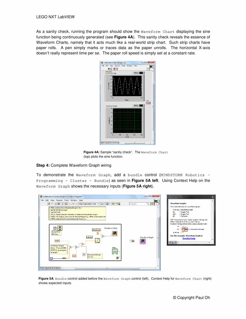
Step 3: Complete Waveform Chart wiring and Test run

Next, add the sine control (MINDSTORMS Robotics – Programming – Numeric –

Trigonometric Functions – sin) and complete wiring as shown in Figure 3A. The end

result is a sine function with amplitude of 5 and frequency of 10 Hz. Note that the while-loop

index variable i multiples a constant of 0.005 to create the elapsed time variable n.

Figure 3 goes here

Figure 2A: Add Wait and Multiply controls, and associated numeric constants to the block diagram. These

controls are building towards the � sin�2�� function.

Figure 3A: Add the sine control and wire to the Waveform Chart

LEGO NXT LabVIEW


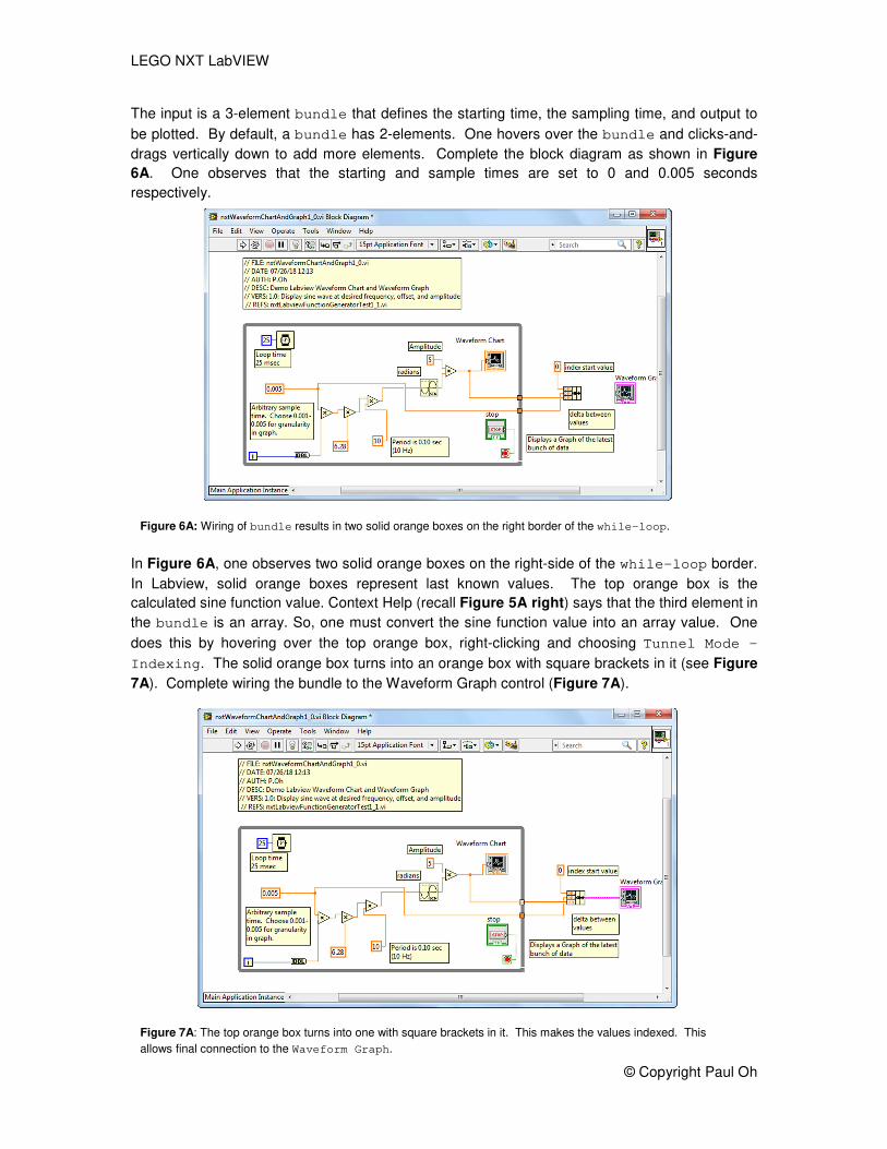
As a sanity check, running the program should show the Waveform Chart displaying the sine

function being continuously generated (see Figure 4A). This sanity check reveals the essence of

Waveform Charts, namely that it acts much like a real-world strip chart. Such strip charts have

paper rolls. A pen simply marks or traces data as the paper unrolls. The horizontal X-axis

doesn’t really represent time per se. The paper roll speed is simply set at a constant rate.

Step 4: Complete Waveform Graph wiring

To demonstrate the Waveform Graph, add a bundle control (MINDSTORM Robotics –

Programming – Cluster – Bundle) as seen in Figure 5A left. Using Context Help on the

Waveform Graph shows the necessary inputs (Figure 5A right).

Figure 4A: Sample “sanity check”. The Waveform Chart

(top) plots the sine function.

Figure 5A: Bundle control added before the Waveform Graph control (left). Context Help for Waveform Chart (right)

shows expected inputs

LEGO NXT LabVIEW


The input is a 3-element bundle that defines the starting time, the sampling time, and output to

be plotted. By default, a bundle has 2-elements. One hovers over the bundle and clicks-and-

drags vertically down to add more elements. Complete the block diagram as shown in Figure

6A. One observes that the starting and sample times are set to 0 and 0.005 seconds

respectively.

In Figure 6A, one observes two solid orange boxes on the right-side of the while-loop border.

In Labview, solid orange boxes represent last known values. The top orange box is the

calculated sine function value. Context Help (recall Figure 5A right) says that the third element in

the bundle is an array. So, one must convert the sine function value into an array value. One

does this by hovering over the top orange box, right-clicking and choosing Tunnel Mode –

Indexing. The solid orange box turns into an orange box with square brackets in it (see Figure

7A). Complete wiring the bundle to the Waveform Graph control (Figure 7A).

Figure 6A: Wiring of bundle results in two solid orange boxes on the right border of the while-loop.

Figure 7A: The top orange box turns into one with square brackets in it. This makes the values indexed. This

allows final connection to the Waveform Graph.

LEGO NXT LabVIEW


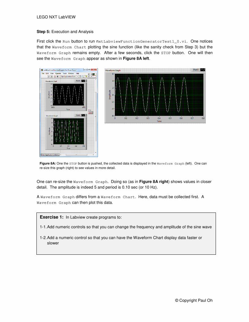
Step 5: Execution and Analysis

First click the Run button to run nxtLabviewFunctionGeneratorTest1_0.vi. One notices

that the Waveform Chart plotting the sine function (like the sanity check from Step 3) but the

Waveform Graph remains empty. After a few seconds, click the STOP button. One will then

see the Waveform Graph appear as shown in Figure 8A left.

One can re-size the Waveform Graph. Doing so (as in Figure 8A right) shows values in closer

detail. The amplitude is indeed 5 and period is 0.10 sec (or 10 Hz).

A Waveform Graph differs from a Waveform Chart. Here, data must be collected first. A

Waveform Graph can then plot this data.

Figure 8A: One the STOP button is pushed, the collected data is displayed in the Waveform Graph (left). One can

re-size this graph (right) to see values in more detail.

Exercise 1: In Labview create programs to:

1-1. Add numeric controls so that you can change the frequency and amplitude of the sine wave

1-2. Add a numeric control so that you can have the Waveform Chart display data faster or

slower

LEGO NXT LabVIEW


Concept 2: Labview XY Graphs

As its name suggests, the XY Graph is used to display relationships. The XY Graph control

receives array elements as inputs. These elements typically come from creating a Bundle.


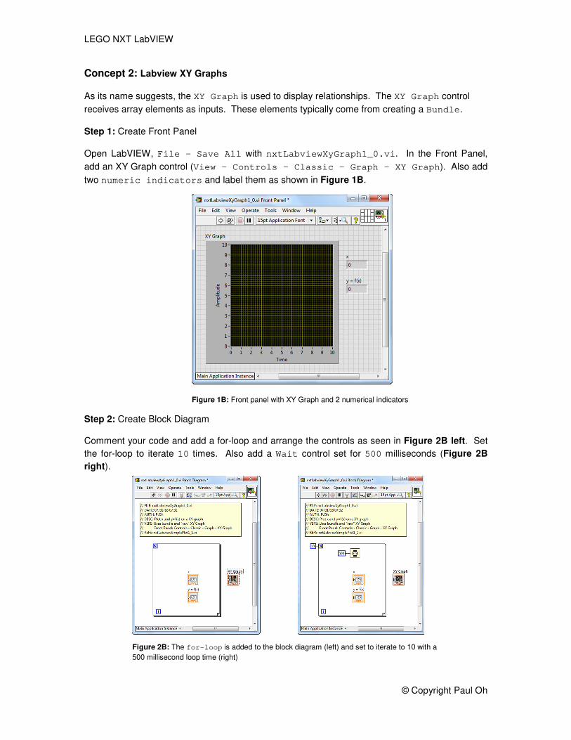
Open LabVIEW, File – Save All with nxtLabviewXyGraph1_0.vi. In the Front Panel,

add an XY Graph control (View – Controls – Classic – Graph – XY Graph). Also add

two numeric indicators and label them as shown in Figure 1B.


Comment your code and add a for-loop and arrange the controls as seen in Figure 2B left. Set

the for-loop to iterate 10 times. Also add a Wait control set for 500 milliseconds (Figure 2B

right).

Figure 1B: Front panel with XY Graph and 2 numerical indicators

Figure 2B: The for-loop is added to the block diagram (left) and set to iterate to 10 with a

500 millisecond loop time (right)

LEGO NXT LabVIEW


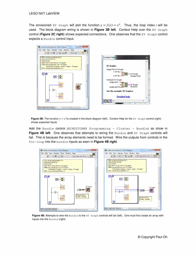
The envisioned XY Graph will plot the function � � � � �. Thus, the loop index � will be

used. The block diagram wiring is shown in Figure 3B left. Context Help over the XY Graph

control (Figure 2C right) shows expected connections. One observes that the XY Graph control

expects a Bundle control input.

Add the Bundle control (MINDSTORMS Programming – Cluster – Bundle) as show in

Figure 4B left. One observes that attempts to wiring the Bundle and XY Graph controls will

fail. This is because the array elements need to be formed. Wire the outputs from controls in the

for-loop into the bundle inputs as seen in Figure 4B right.

Figure 3B: The function � � �is created in the block diagram (left). Context Help for the XY Graph control (right)

shows expected inputs

Figure 4B: Attempts to wire the Bundle to the XY Graph controls will fail (left). One must first create an array with

inputs into the Bundle (right)

LEGO NXT LabVIEW


Step 3: Execution

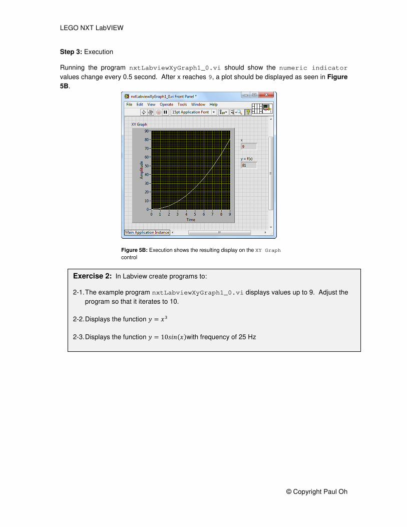
Running the program nxtLabviewXyGraph1_0.vi should show the numeric indicator

values change every 0.5 second. After x reaches 9, a plot should be displayed as seen in Figure

5B.


2-1. The example program nxtLabviewXyGraph1_0.vi displays values up to 9. Adjust the

program so that it iterates to 10.

2-2. Displays the function � � �

2-3. Displays the function � � 10�� with frequency of 25 Hz

Figure 5B: Execution shows the resulting display on the XY Graph

control

LEGO NXT LabVIEW


Concept 3: Writing to File

Often, one would like to save data to a file, which can then be analyzed in Excel. CSV (comma

separated values) is a typical format.


Save Concept 2’s nxtLabviewXyGraph1_0.vi with a new file name as

nxtLabviewFileWriting1_0.vi.


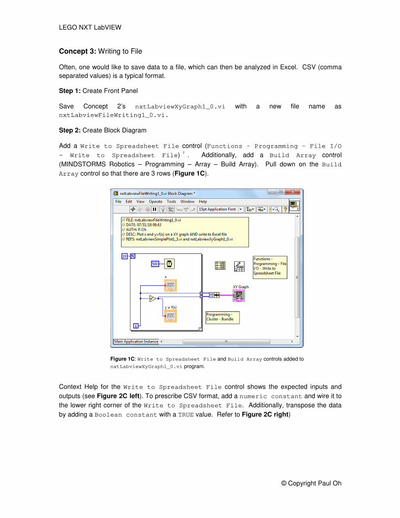
Add a Write to Spreadsheet File control (Functions – Programming – File I/O

– Write to Spreadsheet File)i

. Additionally, add a Build Array control

(MINDSTORMS Robotics – Programming – Array – Build Array). Pull down on the Build

Array control so that there are 3 rows (Figure 1C).

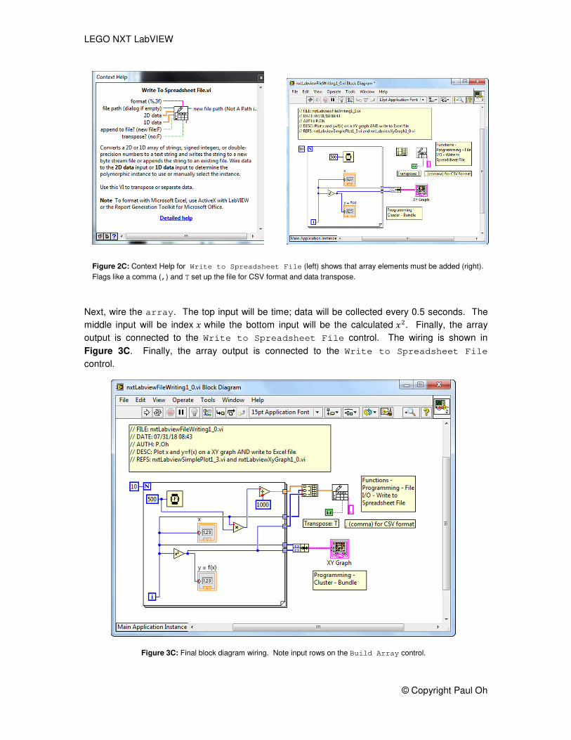
Context Help for the Write to Spreadsheet File control shows the expected inputs and

outputs (see Figure 2C left). To prescribe CSV format, add a numeric constant and wire it to

the lower right corner of the Write to Spreadsheet File. Additionally, transpose the data

by adding a Boolean constant with a TRUE value. Refer to Figure 2C right)

Figure 1C: Write to Spreadsheet File and Build Array controls added to

nxtLabviewXyGraph1_0.vi program.

LEGO NXT LabVIEW


Next, wire the array. The top input will be time; data will be collected every 0.5 seconds. The

middle input will be index while the bottom input will be the calculated �. Finally, the array

output is connected to the Write to Spreadsheet File control. The wiring is shown in

Figure 3C. Finally, the array output is connected to the Write to Spreadsheet File

control.

Figure 2C: Context Help for Write to Spreadsheet File (left) shows that array elements must be added (right).

Flags like a comma (,) and T set up the file for CSV format and data transpose.

Figure 3C: Final block diagram wiring. Note input rows on the Build Array control.

LEGO NXT LabVIEW


Step 3: Execution

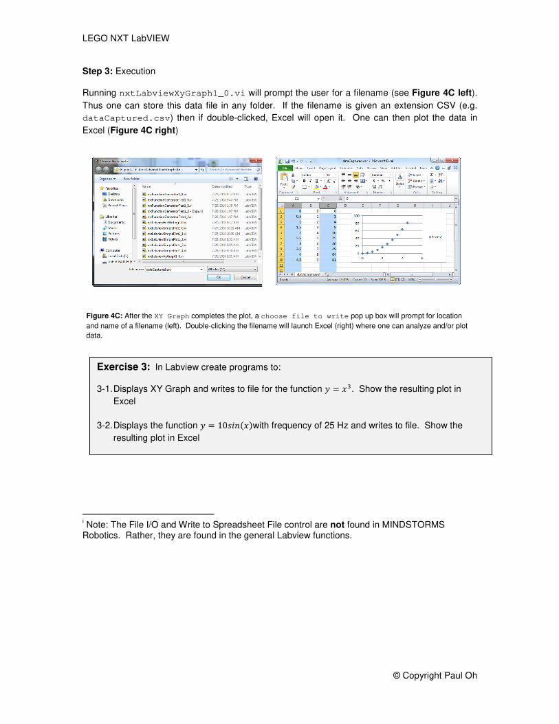
Running nxtLabviewXyGraph1_0.vi will prompt the user for a filename (see Figure 4C left).

Thus one can store this data file in any folder. If the filename is given an extension CSV (e.g.

dataCaptured.csv) then if double-clicked, Excel will open it. One can then plot the data in

Excel (Figure 4C right)

i Note: The File I/O and Write to Spreadsheet File control are not found in MINDSTORMS Robotics. Rather, they are found in the general Labview functions.

Figure 4C: After the XY Graph completes the plot, a choose file to write pop up box will prompt for location

and name of a filename (left). Double-clicking the filename will launch Excel (right) where one can analyze and/or plot

data.


3-1. Displays XY Graph and writes to file for the function � � �. Show the resulting plot in

Excel

3-2. Displays the function � � 10�� with frequency of 25 Hz and writes to file. Show the

resulting plot in Excel

Hands-on Lab: LabVIEW – Charts, Graphs and Files Concept 1 ...€¦ · LabVIEW – Charts, Graphs...

Documents

Transcript of Hands-on Lab: LabVIEW – Charts, Graphs and Files Concept 1 ...€¦ · LabVIEW – Charts, Graphs...