Hands-on integrated CFD educational interface for ...user.engineering.uiowa.edu/~me_160/2017/CFD...
33
Int. J. Aerodynamics, Vol. 2, Nos. 2/3/4, 2012 339 Copyright © 2012 Inderscience Enterprises Ltd. Hands-on integrated CFD educational interface for introductory fluids mechanics Frederick Stern* Department of Mechanical and Industrial Engineering, The University of Iowa, 223C SHL, Iowa City, IA, 52242, USA E-mail: [email protected] *Corresponding author Hyunse Yoon IIHR-Hydroscience and Engineering, The University of Iowa, 223B-2 SHL, Iowa City, IA, 52242, USA E-mail: [email protected] Donald Yarbrough Department of Psychological and Quantitative Foundations, The University of Iowa, 210 Linguist Center, Iowa City, IA, 52242, USA E-mail: [email protected] Murat Okcay, Bilgehan Uygar Oztekin and Breigh Roszelle Interactive Flow Studies Corporation, P.O. Box 784, Waterloo, IA, 50704, USA E-mail: [email protected] E-mail: [email protected] E-mail: [email protected] Abstract: The development, implementation, and evaluation of an effective curriculum for students to learn integrated computational fluid dynamics (CFD) and experimental fluid dynamics (EFD) is described. The CFD objective is to teach students CFD methodology and procedures through a step-by-step CFD process using a CFD educational interface for hands-on student experience. The EFD objective is to teach students use of modern facilities, measurement systems including ePIV and Flowcoach, and uncertainty analysis (UA), following a step-by-step EFD process for fluids engineering experiments. Students analyse and relate CFD and EFD results to fluid physics and classroom lectures, including teamwork and presentation of results. Implementation is described based on results for an introductory level fluid mechanics course, which includes integrated CFD and EFD laboratories for the same geometries and conditions. An independent evaluation investigates and reports the learning outcomes and the effectiveness of the CFD educational interface, ePIV, Flowcoach and CFD and EFD laboratories.
Transcript of Hands-on integrated CFD educational interface for ...user.engineering.uiowa.edu/~me_160/2017/CFD...
Int. J. Aerodynamics, Vol. 2, Nos. 2/3/4, 2012 339
Copyright © 2012 Inderscience Enterprises Ltd.
Hands-on integrated CFD educational interface for introductory fluids mechanics
Frederick Stern* Department of Mechanical and Industrial Engineering, The University of Iowa, 223C SHL, Iowa City, IA, 52242, USA E-mail: [email protected] *Corresponding author
Hyunse Yoon IIHR-Hydroscience and Engineering, The University of Iowa, 223B-2 SHL, Iowa City, IA, 52242, USA E-mail: [email protected]
Donald Yarbrough Department of Psychological and Quantitative Foundations, The University of Iowa, 210 Linguist Center, Iowa City, IA, 52242, USA E-mail: [email protected]
Murat Okcay, Bilgehan Uygar Oztekin and Breigh Roszelle Interactive Flow Studies Corporation, P.O. Box 784, Waterloo, IA, 50704, USA E-mail: [email protected] E-mail: [email protected] E-mail: [email protected]
Abstract: The development, implementation, and evaluation of an effective curriculum for students to learn integrated computational fluid dynamics (CFD) and experimental fluid dynamics (EFD) is described. The CFD objective is to teach students CFD methodology and procedures through a step-by-step CFD process using a CFD educational interface for hands-on student experience. The EFD objective is to teach students use of modern facilities, measurement systems including ePIV and Flowcoach, and uncertainty analysis (UA), following a step-by-step EFD process for fluids engineering experiments. Students analyse and relate CFD and EFD results to fluid physics and classroom lectures, including teamwork and presentation of results. Implementation is described based on results for an introductory level fluid mechanics course, which includes integrated CFD and EFD laboratories for the same geometries and conditions. An independent evaluation investigates and reports the learning outcomes and the effectiveness of the CFD educational interface, ePIV, Flowcoach and CFD and EFD laboratories.

340 F. Stern et al.
Keywords: hands-on labs; integrated CFD and EFD; CFD educational interface; CFD process; EFD process; ePIV; Flowcoach; uncertainty analysis; course evaluation.
Reference to this paper should be made as follows: Stern, F., Yoon, H., Yarbrough, D., Okcay, M., Oztekin, B.U. and Roszelle, B. (2012) ‘Hands-on integrated CFD educational interface for introductory fluids mechanics’, Int. J. Aerodynamics, Vol. 2, Nos. 2/3/4, pp.339–371.
Biographical notes: Frederick Stern is a Professor of the Department of Mechanical and Industrial Engineering, The University of Iowa, Iowa City, IA, USA.
Hyunse Yoon is a Postdoctoral Research Scholar in the IIHR-Hydroscience and Engineering, The University of Iowa, Iowa City, IA, USA.
Donald Yarbrough is a Professor of the Department of Psychological and Quantitative Foundations, The University of Iowa, Iowa City, IA, USA.
Murat Okcay is the CEO of the Interactive Flow Studies Corporation, Waterloo, IA, USA.
Bilgehan Uygar Oztekin is the CTO of the Interactive Flow Studies Corporation, Waterloo, IA, USA.
Breigh Roszelle is a Senior Engineer of the Interactive Flow Studies Corporation, Waterloo, IA, USA.
This paper is a revised version of AIAA Paper 2012-0908 previously presented at an AIAA conference.
1 Introduction
It is well understood that the use of interactive learning is an important part of an engineering education (Feisel and Rosa, 2005). As technology grows and advances it provides new opportunities for well-rounded and meaningful classroom and laboratory student experiences. Multiple studies have found that computer modelling, electronic learning modules, and hands-on experiments lead to an increase in student understanding when applied to engineering courses (Fraser et al., 2007; Keith et al., 2008; Okamoto et al., 2009; Budny and Torick, 2010). For example, Okamoto et al. (2009) developed a novel thermal management of electronics course that combined a standard lecture with both computer modelling and hands-on experiments. They found that students showed a significant improvement in their understanding of the topics, as well as an increase in their ability to confidently perform related tasks. Likewise, Keith et al. (2008) found that using electronic modules was a successful method for teaching chemical engineering students about fuel cells.
This use of technology has often been applied to fluid dynamics courses, where the use of experimental fluid dynamics (EFD) and computational fluid dynamics (CFD),
Hands-on integrated CFD educational interface 341
either alone or in combination, have led to improved student understanding (Fraser et al., 2007; Budny and Torick, 2010; Stern et al., 2006; Sert and Nakboglu, 2007; Van Ransbeeck et al., 2009). An example of this is Fraser et al. (2007) who found that students showed significant improvement in areas they found most difficult when a computer simulation was used to help explain the concepts. Van Ransbeeck et al. (2009) used a combination of EFD and CFD methods, which allowed students to successfully learn fluid dynamic theories by using a hands-on approach and comparing this to computational models. Such experiences not only help students learn about fluid dynamic theories, but also start to build skills that can be applied in future careers in research or industry, as CFD is becoming a widely used tool. As proposed by Stern et al. (2006) CFD interfaces that are developed as learning tools can help students transition into using more complex codes once they are in industry. The goal of combing these tools is to prepare students to solve real world fluid dynamics problems, improve understanding and gain hands-on skills.
Herein the development, implementation, and evaluation of an effective curriculum for students to learn integrated CFD and EFD including ePIV and Flowcoach in introductory undergraduate level courses and laboratories are described. The CFD objective is to teach students from novice to expert users who are well prepared for engineering practice using a CFD educational interface for hands-on student experience, which mirrors actual engineering practice (Stern et al., 2006). The EFD objective is to teach students use of modern facilities, measurement systems, and uncertainty analysis (UA) following a step-by-step approach, which mirrors the real-life EFD process: setup facility; install model; setup equipment; setup data acquisition; perform calibrations; data acquisition, analysis and reduction; and UA, and comparison CFD and/or analytical fluid dynamics (AFD) results (Stern et al., 2004a). Implementation is described based on results of an introductory level fluid mechanics course, which includes integrated CFD and EFD laboratories for the same geometries and conditions. An collaborative (internal and external) evaluation (Yarbrough et al., 2011) investigates and reports the learning outcomes and the effectiveness of the CFD educational interface, ePIV/Flowcoach and CFD and EFD laboratories. Stern et al. (2006) describes development, implementation, and evaluation of the CFD educational interface in intermediate level courses.
2 Introductory fluids course with EFD and CFD laboratories
2.1 Design
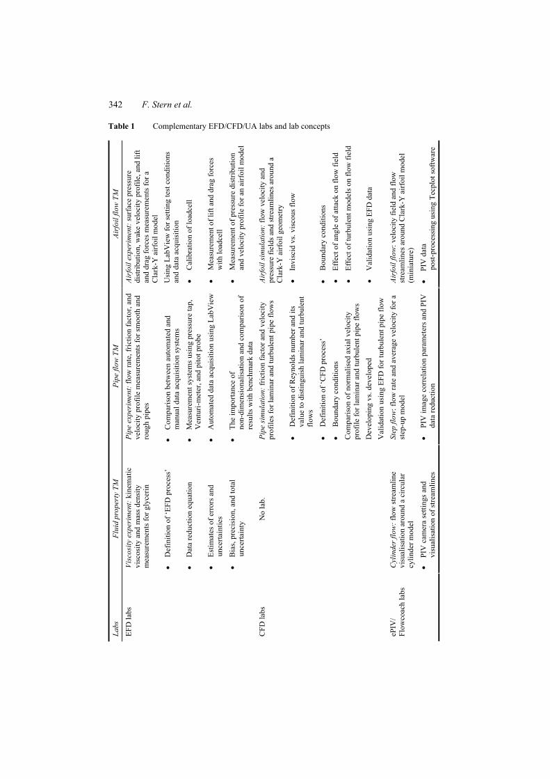
The introductory fluid mechanics course at the University of Iowa is a four-semester-hour course, offered as a requisite course to junior level Mechanical Engineering and Civil and Environmental Engineering students and often elected by Biomedical Engineering students. Typically about one hundred students are enrolled in the course each semester. The course consists of classroom lectures and labs. Lectures use textbooks and lecture notes, along with problem solving, with emphasis placed on AFD. Labs include both computational CFD and experimental EFD and ePIV/Flowcoach labs designed to be complementary with each other, as shown in Table 1.
342 F. Stern et al.
Table 1 Complementary EFD/CFD/UA labs and lab concepts
Labs
Fl
uid
prop
erty
TM
Pi
pe fl
ow T
M
Airf
oil f
low
TM
Visc
osity
exp
erim
ent:
kine
mat
ic
visc
osity
and
mas
s de
nsity
m
easu
rem
ents
for g
lyce
rin
Pipe
exp
erim
ent:
flow
rate
, fric
tion
fact
or, a
nd
velo
city
pro
file
mea
sure
men
ts fo
r sm
ooth
and
ro
ugh
pipe
s
Airf
oil e
xper
imen
t: su
rfac
e pr
essu
re
dist
ribut
ion,
wak
e ve
loci
ty p
rofil
e, a
nd li
ft an
d dr
ag fo
rces
mea
sure
men
ts fo
r a
Cla
rk-Y
airf
oil m
odel
• D
efin
ition
of ‘
EFD
pro
cess
’ •
Com
paris
on b
etw
een
auto
mat
ed a
nd
man
ual d
ata
acqu
isiti
on sy
stem
s U
sing
Lab
Vie
w fo
r set
ting
test
con
ditio
ns
and
data
acq
uisi
tion
• D
ata
redu
ctio
n eq
uatio
n •
Mea
sure
men
t sys
tem
s us
ing
pres
sure
tap,
V
entu
ri-m
eter
, and
pito
t pro
be
• C
alib
ratio
n of
load
cell
• Es
timat
es o
f err
ors
and
unce
rtain
ties
• A
utom
ated
dat
a ac
quis
ition
usi
ng L
abV
iew
•
Mea
sure
men
t of l
ift a
nd d
rag
forc
es
with
load
cell
EFD
labs
• B
ias,
pre
cisi
on, a
nd to
tal
unce
rtain
ty
• Th
e im
porta
nce
of
non-
dim
ensi
onal
isat
ion
and
com
paris
on o
f re
sults
with
ben
chm
ark
data
• M
easu
rem
ent o
f pre
ssur
e di
strib
utio
n an
d ve
loci
ty p
rofil
e fo
r an
airf
oil m
odel
Pipe
sim
ulat
ion:
fric
tion
fact
or a
nd v
eloc
ity
prof
iles f
or la
min
ar a
nd tu
rbul
ent p
ipe
flow
s Ai
rfoi
l sim
ulat
ion:
flow
vel
ocity
and
pr
essu
re fi
elds
and
stre
amlin
es a
roun
d a
Cla
rk-Y
airf
oil g
eom
etry
• D
efin
ition
of R
eyno
lds n
umbe
r and
its
valu
e to
dis
tingu
ish
lam
inar
and
turb
ulen
t flo
ws
• In
visc
id v
s. vi
scou
s flo
w
• D
efin
ition
of ‘
CFD
pro
cess
’ •
Bou
ndar
y co
nditi
ons
• B
ound
ary
cond
ition
s •
Effe
ct o
f ang
le o
f atta
ck o
n flo
w fi
eld
Com
paris
on o
f nor
mal
ised
axi
al v
eloc
ity
prof
ile fo
r lam
inar
and
turb
ulen
t pip
e flo
ws
• Ef
fect
of t
urbu
lent
mod
els o
n flo
w fi
eld
Dev
elop
ing
vs. d
evel
oped
CFD
labs
N
o la
b.
Val
idat
ion
usin
g EF
D fo
r tur
bule
nt p
ipe
flow
•
Val
idat
ion
usin
g EF
D d
ata
Cyl
inde
r flo
w: f
low
stre
amlin
e vi
sual
isat
ion
arou
nd a
circ
ular
cy
linde
r mod
el
Step
flow
: flo
w ra
te a
nd a
vera
ge v
eloc
ity fo
r a
step
-up
mod
el
Airf
oil f
low
: vel
ocity
fiel
d an
d flo
w
stre
amlin
es a
roun
d C
lark
-Y a
irfoi
l mod
el
(min
iatu
re)
ePIV
/ Fl
owco
ach
labs
• PI
V c
amer
a se
tting
s an
d vi
sual
isat
ion
of st
ream
lines
•
PIV
imag
e co
rrel
atio
n pa
ram
eter
s and
PIV
da
ta re
duct
ion
• PI
V d
ata
po
st-p
roce
ssin
g us
ing
Tecp
lot s
oftw
are
Hands-on integrated CFD educational interface 343
The present course is founded on a long history of fluid mechanics education at the University of Iowa. Before 1985, the course was mainly textbook-based classroom lectures (four lectures per week) with focus on analytical solution methods and a few experimental labs for highlighting fundamental principles. Subsequently, a wind tunnel was designed and constructed for research quality experiments using modern measurement systems along with complementary student-run potential-flow panel code for comparison with their experimental data, which had favourable learning outcomes and student responses. The concept was expanded during the 1990s by restructuring the course for three-semester hours of AFD (three lectures per week) and one-semester hour (one laboratory meeting per week) for complementary EFD, CFD, and UA laboratories. EFD labs were improved and UA was introduced. Complementary CFD labs were also introduced using an advanced research code modified for limited user options. From 1999 to 2002, the research CFD code was replaced by the commercial CFD software (FLUENT) and refinements were made and the overall approach was used as a proof of concept for the initiation of a three-year National Science Foundation sponsored Course, Curriculum and Laboratory Improvement – Educational Materials Development project Integration of Simulation Technology into Undergraduate Engineering Courses and Laboratories (ISTUE) with faculty partners from colleges of engineering at Iowa, Iowa State, Cornell and Howard universities along with industrial (commercial CFD) partner FLUENT Inc. The ISTUE project focused on the development of a common CFD educational interface and teaching modules (TM) for its use for the faculty partners’ respective courses and laboratories. Evaluations confirmed that the implementation was successful but at same time indicated directions for improvements. Students anonymous responses suggested that they agreed the EFD, CFD, and UA labs were helpful for learning fluid mechanics and important tools that they may need as professional engineers in the future; however, they would like their learning experience to be as hands-on as possible. During 2003, additional improvements were made for hands-on complementary EFD/CFD/UA labs. Hands-on is defined as the use of EFD, CFD, and UA engineering tools in meaningful learning experiences, which mirror as much as possible the real-life engineering practice. The most recent improvement was made during 2008 to 2010 by adding complementary ePIV/Flowcoach experiments to the EFD labs.
As a first course in fluid mechanics it provides an introduction to basic concepts in fluid statics, kinematics, and dynamics. Control volume and differential equation and dimensional analysis methods are derived and used to demonstrate applications to simple external- and internal-flow fluids engineering systems to determine variables of interest (pressure; shear stress; velocity distributions; flow rates; forces; energy losses; power requirements; etc.). Homework assignments, tests, and complementary experimental and CFD (EFD and CFD) laboratories are integrated into the course to reinforce the theory and its practical application. The EFD laboratories introduce fluids engineering facilities, measurement systems (equipment and data acquisition and reduction methods) and uncertainty assessment methodology and procedures. The CFD laboratories introduce fluids engineering simulation-based design methods, utilising the CFD educational interface. Three TM’s were developed for complementary EFD and CFD labs: fluid property (EFD only) and pipe and airfoil flow (EFD and CFD). Concepts were developed for classroom lectures and the EFD and
344 F. Stern et al.
CFD labs. The classroom lecture concepts are cross-referenced to the homework and exams.
TM consists of the lab purpose and concepts, educational materials, lab report instructions, pre-lab questions, lab lecture, exercise notes and data reduction sheets for each EFD and CFD lab. For the fluid property TM, the purpose is hands-on student experience with table-top facility and simple measurement system for fluid property measurement, including comparison manufacturer values and rigorous implementation standard EFD UA. For the pipe flow TM the purpose is hands-on student experience with complementary EFD, CFD, and UA for introductory pipe flow, including friction factor and mean velocity measurements and comparisons benchmark data, laminar and turbulent flow CFD simulations, modelling and numerical methods and verification studies, and validation using AFD and EFD. For the airfoil TM the purpose is hands-on student experience with complementary EFD, CFD, and UA for introductory airfoil flow, including lift and drag, surface pressure, and mean and turbulent wake velocity profile measurements and comparisons benchmark data, inviscid and turbulent flow simulations, modelling and numerical methods and verification studies, and validation using AFD and EFD.
2.2 Course and problem solving learning objectives
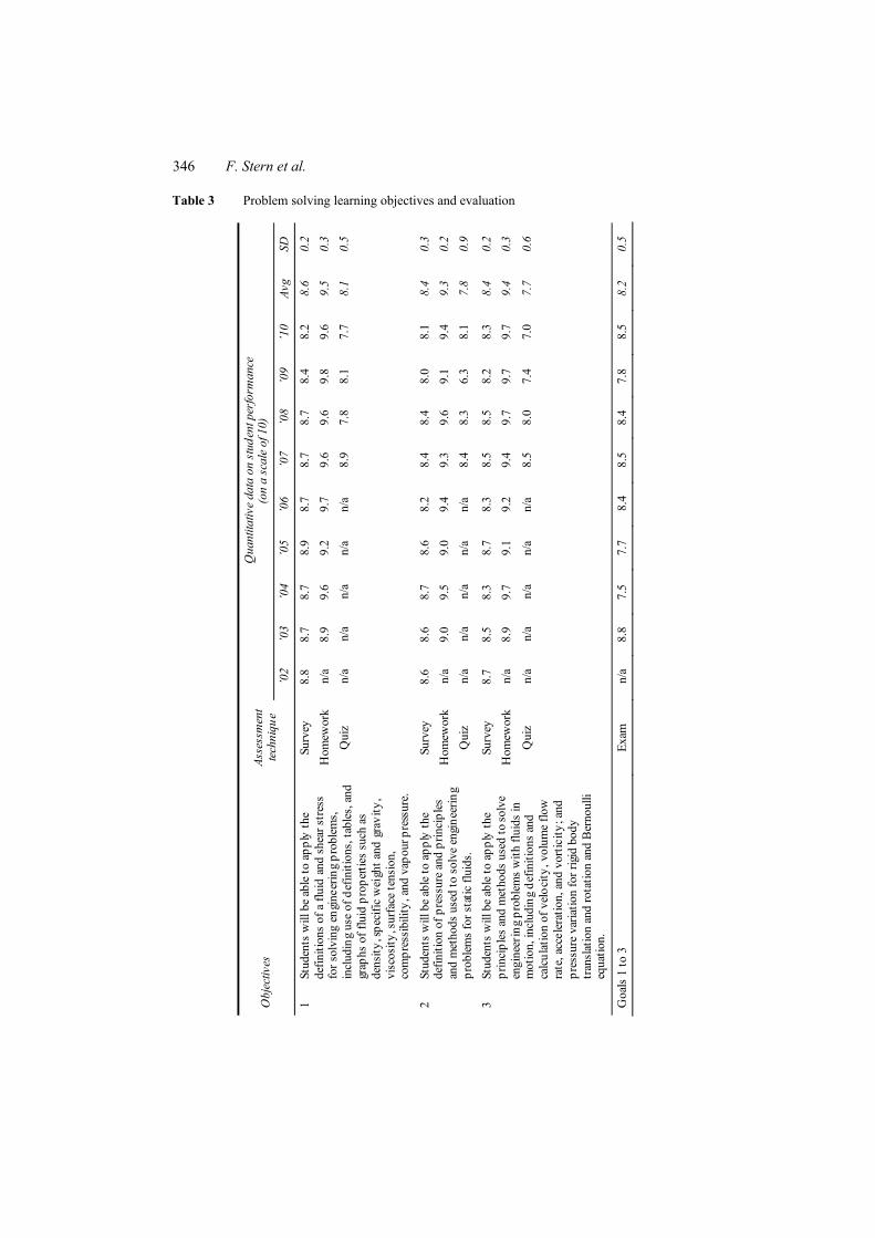
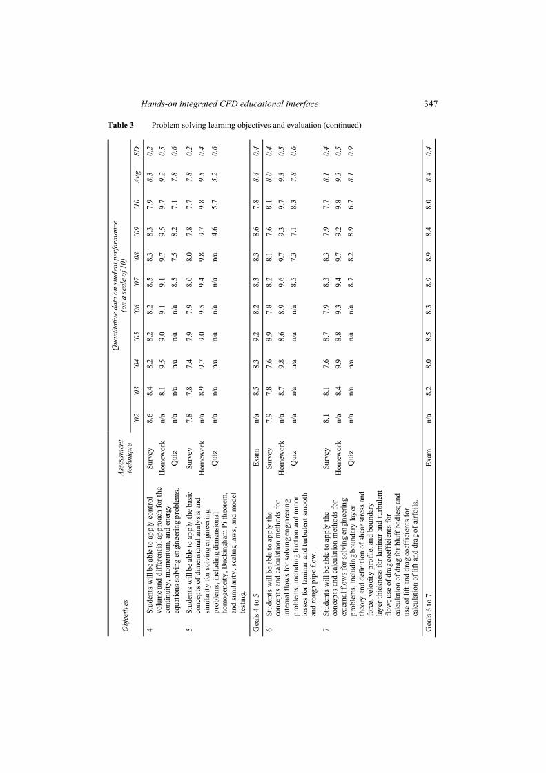
The course general learning objectives are listed in Table 2. Eight objectives were developed based on the classroom lecture and EFD and CFD lab concepts covering the student’s learning experience, complementary EFD and CFD laboratories, student evaluation and class website. The end-of-semester survey is used for assessment. The problem solving learning objectives are listed in Table 3. Seven objectives were developed based on the class room lecture concepts covering basic definitions, fluid statics and dynamics, control volume and differential analysis, dimensional analysis, and applications for internal and external flows. Homework, quizzes, exams and the survey are used for assessment. The assessment techniques and instruments as well as analysis procedures as summarised in Tables 2 through 6 are described more fully in Section 6, Assessment and Evaluation.
2.3 Implementation
The class website (http://www.engineering.uiowa.edu/~fluids/) provides all course materials, including lecture notes, EFD and CFD lab handouts and assignments, and grades for homework, laboratory reports, and tests. Lectures present website lecture notes, etc. with additional discussion, using an overhead projector. Students should not take detailed in-class notes copying this material since it is available and can be downloaded and printed via the website, but should rather augment website material with notes based on additional discussion, which supplement and expand on website material.

Hands-on integrated CFD educational interface 345
Table 2 Course general learning objectives and evaluation
Qua
ntita
tive
data
on
stud
ent p
erfo
rman
ce
(on
a sc
ale
of 1
0)
Obj
ectiv
es
Asse
ssm
ent
tech
niqu
e ’0
2 ’0
3 ’0
4 ’0
5 ’0
6 ’0
7 ’0
8 ’0
9 ’1
0 Av
g SD
1 St
uden
ts in
gen
eral
will
enj
oy th
eir l
earn
ing
expe
rienc
e in
this
cou
rse
Surv
ey
7.9
8.2
n/a
n/a
n/a
8.2
7.5
7.0
6.7
7.6
0.6
2 Ex
perim
enta
l flu
id d
ynam
ics (
EFD
), co
mpu
tatio
nal f
luid
dyn
amic
s (C
FD),
and
unce
rtain
ty a
naly
sis (
UA
), cl
assr
oom
and
pr
e-la
b le
ctur
es w
ill e
ffec
tivel
y pr
epar
e st
uden
ts
for ‘
hand
s-on
’ lab
orat
ory
expe
rienc
e.
Surv
ey
6.7
6.5
n/a
n/a
n/a
8.8
7.8
7.1
7.4
7.4
0.8
3 ‘H
ands
-on’
labo
rato
ry e
xper
ienc
e w
ill u
se E
FD,
CFD
, and
UA
as e
ngin
eerin
g to
ols i
n a
mea
ning
ful l
earn
ing
expe
rienc
e.
Surv
ey
n/a
6.4
n/a
n/a
n/a
8.5
8.0
7.5
7.8
7.6
0.7
4 ‘H
ands
-on’
labo
rato
ry e
xper
ienc
e w
ill m
irror
as
muc
h as
pos
sibl
e th
e ‘r
eal-l
ife’ e
ngin
eerin
g pr
actic
e.
Surv
ey
n/a
n/a
n/a
n/a
n/a
8.8
7.2
6.9
7.1
7.5
0.8
5 Th
e la
b co
nten
t and
skill
dev
elop
men
t will
ef
fect
ivel
y m
atch
stud
ents
’ lea
rnin
g ne
eds,
incl
udin
g pr
ior k
now
ledg
e an
d sk
ill, s
tude
nt
obje
ctiv
es fo
r sel
f-de
velo
pmen
t as e
ngin
eers
, and
st
uden
t dis
posi
tions
and
lear
ning
styl
es.
Surv
ey
7.7
7.3
n/a
n/a
n/a
9.0
7.4
7.3
7.1
7.6
0.6
6 St
uden
ts’ e
valu
atio
n th
roug
h ho
mew
ork,
test
s, an
d pr
e-la
b an
d la
bora
tory
repo
rts w
ill b
e fa
ir,
accu
rate
, pro
per,
feas
ible
, and
use
ful.
Surv
ey
8.0
8.2
n/a
n/a
n/a
8.8
7.7
7.9
7.6
8.0
0.4
7 Ev
alua
tions
in th
is c
ours
e w
ill a
llow
stud
ents
to
show
wha
t the
y kn
ow a
nd c
an d
o, a
s rel
ated
to
expe
cted
cou
rse
outc
omes
.
Surv
ey
7.9
8.0
n/a
n/a
n/a
8.4
7.8
7.5
7.6
7.9
0.3
8 Th
e w
ebsi
te w
ill b
e us
eful
for l
earn
ing
in th
is
cour
se, i
nclu
ding
pos
ting
clas
s inf
orm
atio
n,
new
s, sc
hedu
le, l
ectu
re n
otes
, EFD
/CFD
lab
mat
eria
ls, h
omew
ork
and
test
solu
tions
, gra
des,
imag
e ga
llery
, and
link
s.
Surv
ey
9.2
8.7
n/a
n/a
n/a
8.5
8.8
8.5
8.3
8.7
0.3
346 F. Stern et al.
Table 3 Problem solving learning objectives and evaluation
Qua
ntita
tive
data
on
stud
ent p
erfo
rman
ce
(on
a sc
ale
of 1
0)
Obj
ectiv
es
Asse
ssm
ent
tech
niqu
e ’0
2 ’0
3 ’0
4 ’0
5 ’0
6 ’0
7 ’0
8 ’0
9 ’1
0 Av
g SD
Surv
ey
8.8
8.7
8.7
8.9
8.7
8.7
8.7
8.4
8.2
8.6
0.2
Hom
ewor
k n/
a 8.
9 9.
6 9.
2 9.
7 9.
6 9.
6 9.
8 9.
6 9.
5 0.
3 1
Stud
ents
will
be
able
to a
pply
the
defin
ition
s of
a fl
uid
and
shea
r str
ess
for s
olvi
ng e
ngin
eerin
g pr
oble
ms,
in
clud
ing
use
of d
efin
ition
s, ta
bles
, and
gr
aphs
of f
luid
pro
perti
es s
uch
as
dens
ity, s
peci
fic w
eigh
t and
gra
vity
, vi
scos
ity, s
urfa
ce te
nsio
n,
com
pres
sibi
lity,
and
vap
our p
ress
ure.
Qui
z n/
a n/
a n/
a n/
a n/
a 8.
9 7.
8 8.
1 7.
7 8.
1 0.
5
Surv
ey
8.6
8.6
8.7
8.6
8.2
8.4
8.4
8.0
8.1
8.4
0.3
Hom
ewor
k n/
a 9.
0 9.
5 9.
0 9.
4 9.
3 9.
6 9.
1 9.
4 9.
3 0.
2 2
Stud
ents
will
be
able
to a
pply
the
defin
ition
of p
ress
ure
and
prin
cipl
es
and
met
hods
use
d to
sol
ve e
ngin
eerin
g pr
oble
ms
for s
tatic
flui
ds.
Qui
z n/
a n/
a n/
a n/
a n/
a 8.
4 8.
3 6.
3 8.
1 7.
8 0.
9
Surv
ey
8.7
8.5
8.3
8.7
8.3
8.5
8.5
8.2
8.3
8.4
0.2
Hom
ewor
k n/
a 8.
9 9.
7 9.
1 9.
2 9.
4 9.
7 9.
7 9.
7 9.
4 0.
3 3
Stud
ents
will
be
able
to a
pply
the
prin
cipl
es a
nd m
etho
ds u
sed
to so
lve
engi
neer
ing
prob
lem
s w
ith fl
uids
in
mot
ion,
incl
udin
g de
finiti
ons
and
calc
ulat
ion
of v
eloc
ity, v
olum
e flo
w
rate
, acc
eler
atio
n, a
nd v
ortic
ity; a
nd
pres
sure
var
iatio
n fo
r rig
id b
ody
tran
slat
ion
and
rota
tion
and
Ber
noul
li eq
uatio
n.
Qui
z n/
a n/
a n/
a n/
a n/
a 8.
5 8.
0 7.
4 7.
0 7.
7 0.
6
Goa
ls 1
to 3
Ex
am
n/a
8.8
7.5
7.7
8.4
8.5
8.4
7.8
8.5
8.2
0.5
Hands-on integrated CFD educational interface 347
Table 3 Problem solving learning objectives and evaluation (continued)
Qua
ntita
tive
data
on
stud
ent p
erfo
rman
ce
(on
a sc
ale
of 1
0)
Obj
ectiv
es
Asse
ssm
ent
tech
niqu
e ’0
2 ’0
3 ’0
4 ’0
5 ’0
6 ’0
7 ’0
8 ’0
9 ’1
0 Av
g SD
Surv
ey
8.6
8.4
8.2
8.2
8.2
8.5
8.3
8.3
7.9
8.3
0.2
Hom
ewor
k n/
a 8.
1 9.
5 9.
0 9.
1 9.
1 9.
7 9.
5 9.
7 9.
2 0.
5 4
Stud
ents
will
be
able
to a
pply
con
trol
vo
lum
e an
d di
ffer
entia
l app
roac
h fo
r the
co
ntin
uity
, mom
entu
m, a
nd e
nerg
y eq
uatio
ns s
olvi
ng e
ngin
eerin
g pr
oble
ms.
Qui
z n/
a n/
a n/
a n/
a n/
a 8.
5 7.
5 8.
2 7.
1 7.
8 0.
6
Surv
ey
7.8
7.8
7.4
7.9
7.9
8.0
8.0
7.8
7.7
7.8
0.2
Hom
ewor
k n/
a 8.
9 9.
7 9.
0 9.
5 9.
4 9.
8 9.
7 9.
8 9.
5 0.
4 5
Stud
ents
will
be
able
to a
pply
the
basi
c co
ncep
ts o
f dim
ensi
onal
ana
lysi
s an
d si
mila
rity
for s
olvi
ng e
ngin
eerin
g pr
oble
ms,
incl
udin
g di
men
sion
al
hom
ogen
eity
, Buc
king
ham
Pi t
heor
em,
and
sim
ilarit
y, s
calin
g la
ws,
and
mod
el
test
ing.
Qui
z n/
a n/
a n/
a n/
a n/
a n/
a n/
a 4.
6 5.
7 5.
2 0.
6
Goa
ls 4
to 5
Ex
am
n/a
8.5
8.3
9.2
8.2
8.3
8.3
8.6
7.8
8.4
0.4
Surv
ey
7.9
7.8
7.6
8.9
7.8
8.2
8.1
7.6
8.1
8.0
0.4
Hom
ewor
k n/
a 8.
7 9.
8 8.
6 8.
9 9.
6 9.
7 9.
3 9.
7 9.
3 0.
5 6
Stud
ents
will
be
able
to a
pply
the
conc
epts
and
cal
cula
tion
met
hods
for
inte
rnal
flow
s fo
r sol
ving
eng
inee
ring
prob
lem
s, in
clud
ing
fric
tion
and
min
or
loss
es fo
r lam
inar
and
turb
ulen
t sm
ooth
an
d ro
ugh
pipe
flow
.
Qui
z n/
a n/
a n/
a n/
a n/
a 8.
5 7.
3 7.
1 8.
3 7.
8 0.
6
Surv
ey
8.1
8.1
7.6
8.7
7.9
8.3
8.3
7.9
7.7
8.1
0.4
Hom
ewor
k n/
a 8.
4 9.
9 8.
8 9.
3 9.
4 9.
7 9.
2 9.
8 9.
3 0.
5 7
Stud
ents
will
be
able
to a
pply
the
conc
epts
and
cal
cula
tion
met
hods
for
exte
rnal
flow
s fo
r sol
ving
eng
inee
ring
prob
lem
s, in
clud
ing
boun
dary
laye
r th
eory
and
def
initi
on o
f she
ar s
tres
s an
d fo
rce,
vel
ocity
pro
file,
and
bou
ndar
y la
yer t
hick
ness
for l
amin
ar a
nd tu
rbul
ent
flow
; use
of d
rag
coef
fici
ents
for
calc
ulat
ion
of d
rag
for b
luff
bod
ies;
and
us
e of
lift
and
dra
g co
effi
cien
ts fo
r ca
lcul
atio
n of
lift
and
dra
g of
airf
oils
.
Qui
z n/
a n/
a n/
a n/
a n/
a 8.
7 8.
2 8.
9 6.
7 8.
1 0.
9
Goa
ls 6
to 7
Ex
am
n/a
8.2
8.0
8.5
8.3
8.9
8.9
8.4
8.0
8.4
0.4

348 F. Stern et al.
A total 44 classroom lectures are given throughout the semester, three lectures per week and each lecture for 50 minutes. One lecture is used for introducing an overview of AFD, EFD, and CFD as complementary tools of engineering practice at the beginning of the course, and one EFD classroom lecture and one CFD classroom lecture are given before the first EFD and CFD labs, respectively. At the beginning of the EFD and CFD lectures students take a pre-test on the EFD and CFD labs, respectively, and take a post-test on the final lecture day. A few example problems are solved during each lecture and two or three homework problems on similar concepts are assigned, due by next lecture day. Office hours by teaching assistants are provided after each lecture to answer students’ questions on solving the homework problems. In-class pop-quizzes are given randomly approximately every two weeks and a total about ten quizzes through the semester. There are two in-semester 50-minute exams and one final 120-minute exam. All exams are closed-notes and books but one-page formula sheet is allowed to exams. The final course grade is based on the total score points earned during the semester for homework (10%), quiz (15%), exams (50%), and lab reports (25%). A student anonymous survey is also given on the final day.
3 EFD fluids laboratory
3.1 Design
Engineering EFD testing is undergoing change from routine tests for global variables to detailed tests for local variables for model development and CFD validation, as design methodology changes from model testing and AFD to simulation-based design. Detailed testing requires use of modern facilities with advanced measurement systems following standard procedures and UA. Requirements on intervals of uncertainties are even more stringent than required previously since they are a limiting factor in establishing intervals of CFD validation and code certification and ultimately credibility of simulation technology. Also, routine test data is more likely used ‘in-house’ whereas detailed test data is more likely utilised internationally, which puts increased emphasis on standardisation of procedures. Detailed testing offers new opportunities, as amount and complexity of testing is increased.
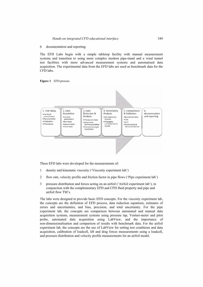
The EFD labs are designed to provide students with hands-on experience with EFD methodology and UA procedures following the EFD Process (Figure 1), which mirrors the real-life engineering practice and guides students smoothly through the labs even for those with less or no experience conducting experiments. The ‘EFD Process’ is a step-by-step procedure:
1 test setup
2 data acquisition
3 data reduction and analysis
4 UA
5 comparisons and validation
Hands-on integrated CFD educational interface 349
6 documentation and reporting.
The EFD Labs begin with a simple tabletop facility with manual measurement systems and transition to using more complex modern pipe-stand and a wind tunnel test facilities with more advanced measurement systems and automatised data acquisition. The experimental data from the EFD labs are used as benchmark data for the CFD labs.
Figure 1 EFD process
Three EFD labs were developed for the measurements of:
1 density and kinematic viscosity (‘Viscosity experiment lab’)
2 flow rate, velocity profile and friction factor in pipe flows (‘Pipe experiment lab’)
3 pressure distribution and forces acting on an airfoil (‘Airfoil experiment lab’), in conjunction with the complementary EFD and CFD fluid property and pipe and airfoil flow TM’s.
The labs were designed to provide basic EFD concepts. For the viscosity experiment lab, the concepts are the definition of EFD process, data reduction equations, estimates of errors and uncertainties, and bias, precision, and total uncertainty. For the pipe experiment lab, the concepts are comparison between automated and manual data acquisition systems, measurement systems using pressure tap, Venturi-meter and pitot probe, automated data acquisition using LabView, and the importance of non-dimensionalisation and comparison of results with benchmark data. For the airfoil experiment lab, the concepts are the use of LabView for setting test conditions and data acquisition, calibration of loadcell, lift and drag forces measurements using a loadcell, and pressure distribution and velocity profile measurements for an airfoil model.

350 F. Stern et al.
Table 4 EFD labs learning objectives and evaluation
Qua
ntita
tive
data
on
stud
ent p
erfo
rman
ce
(on
a sc
ale
of 1
0)
Obj
ectiv
es
Ass
essm
ent
tech
niqu
e ’0
2 ’0
3 ’0
4 ’0
5 ’0
6 ’0
7 ’0
8 ’0
9 ’1
0 A
vg
SD
1 P
rovi
de s
tude
nts
wit
h ‘h
ands
-on’
exp
erie
nce
wit
h E
FD
met
hodo
logy
and
UA
pro
cedu
res
thro
ugh
step
-by
-ste
p a
ppro
ach
follo
win
g E
FD
p
roce
ss: s
etup
fac
ility
, ins
tall
mod
el, s
etup
eq
uip
men
t, s
etup
dat
a ac
quis
itio
n us
ing
Lab
Vie
w, p
erfo
rm c
alib
rati
on, d
ata
anal
ysi
s an
d re
duct
ion,
UA
, and
com
par
ison
wit
h C
FD
an
d/or
AF
D r
esul
ts.
Surv
ey
7.6
7.7
8.2
8.3
8.3
8.2
8.1
7.8
7.8
8.0
0.2
2 St
uden
ts w
ill b
e ab
le t
o co
nduc
t fl
uids
en
gine
erin
g ex
per
imen
ts u
sing
tab
leto
p a
nd
mod
ern
faci
litie
s su
ch a
s p
ipe
stan
ds a
nd w
ind
tunn
els
and
mod
ern
mea
sure
men
t sy
stem
s,
incl
udin
g p
ress
ure
tran
sduc
ers,
pit
ot p
robe
s,
load
cells
, and
co
mp
uter
dat
a ac
quis
itio
n sy
stem
(L
abV
iew
) an
d d
ata
redu
ctio
n.
Surv
ey
8.0
7.8
8.5
8.5
8.3
8.3
8.3
7.5
8.1
8.1
0.4
3 St
uden
ts w
ill b
e ab
le t
o im
ple
men
t E
FD
UA
fo
r p
ract
ical
en
gine
erin
g ex
per
imen
ts.
Surv
ey
7.0
6.8
7.6
7.6
6.6
7.8
7.6
7.0
7.2
7.2
0.5
4 St
uden
ts w
ill b
e ab
le t
o us
e E
FD
dat
a fo
r va
lidat
ion
of C
FD
and
ana
lyti
cal f
luid
dy
nam
ics
(AF
D)
resu
lts.
Surv
ey
8.2
7.7
8.0
8.3
7.3
8.5
8.4
8.0
8.1
8.1
0.4
5 St
uden
ts w
ill b
e ab
le t
o an
aly
se a
nd r
elat
e E
FD
res
ults
to f
luid
phy
sics
and
cla
ssro
om
lect
ures
, inc
lud
ing
team
wor
k an
d p
rese
ntat
ion
of r
esul
ts in
wri
tten
and
gra
phi
cal f
orm
.
Surv
ey
7.9
7.9
8.1
8.3
8.0
8.4
8.1
7.6
7.9
8.0
0.3
Lab
rep
ort
1 n/
a n/
a n/
a 9.
3 8.
4 8.
7 9.
2 8.
6 8.
9 8.
8 0.
4 L
ab r
epor
t 2
n/a
n/a
n/a
9.0
8.4
9.1
9.0
9.0
8.9
8.9
0.3
Lab
rep
ort
3 n/
a n/
a n/
a 9.
3 8.
8 9.
3 8.
8 9.
0 8.
8 8.
9 0.
2 P
re-t
est
n/a
n/a
n/a
5.3
5.5
5.9
5.8
4.8
5.2
5.4
0.4
(Con
fide
nce)
n/
a n/
a n/
a n/
a n/
a n/
a n/
a (3
.7)
(4.3
) (4
.0)
Pos
t-te
st
n/a
n/a
n/a
7.8
7.0
7.1
7.9
7.9
7.1
7.5
0.4
(Con
fide
nce)
n/
a n/
a n/
a n/
a n/
a n/
a n/
a (7
.3)
(6.7
) (7
.0)
Goa
ls 1
to
5
Scor
e in
crea
se
n/a
n/a
n/a
2.5
1.6
1.1
2.2
3.1
1.9
2.0
0.6

Hands-on integrated CFD educational interface 351
3.2 EFD learning objectives
The learning objectives of EFD labs are listed in Table 4. Five objectives were developed based on the lab concepts (Table 1) covering the EFD process, use of modern facilities and measurement systems, UA and relationship classroom lectures and CFD labs. The lab reports, pre/post-test and end-of-the semester survey are used for assessment.
3.3 Implementation
Each EFD lab consists of two laboratory meetings: a pre-lab meeting and a regular lab meeting. Each meeting is for two hours once per week. At the beginning of each lab, a lecture is given for an overview of the experiment: purpose, measurement systems, experimental process, UA methodologies, and relevant fluid dynamics theory. Students are required to read the lecture materials prior to pre-lab meetings and answer the pre-lab questions during the pre-labs in order to familiarise themselves with the lab. Hands-on procedures for the experiment are provided in the exercise notes of each lab. Data reduction sheets (usually Microsoft Excel spreadsheets) are used to facilitate the data analysis and UA. Lab report instructions guide students to write lab reports and can be used by teaching assistants to grade the reports. Students work in groups, typically three to four students, but submit separate lab reports. Specific implementation of each EFD lab is as described below.
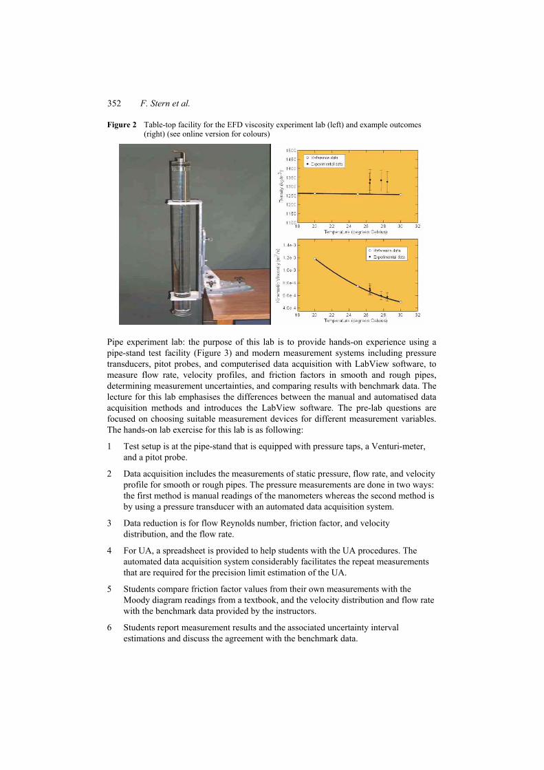
Viscosity experiment lab: the purpose of this lab is to measure fluid properties (density and kinematic viscosity of glycerin) by using a table-top facility (Figure 2) and simple measurement devices. Students compare their measurement results with the manufacturer’s values and implement standard EFD UA. The lab lecture is used to provide the background fluids dynamics theories to derive the equations for fluid density and kinematic viscosity. The standard UA methodology and procedures are also emphasised during this lecture. For pre-lab questions, students derive the equations and consider necessary measurement variables and devices, along with discussions on the bias and precision limits of the measurement. The hands-on lab exercise is by following the EFD process:
1 For test setup students prepare a long acrylic-cylinder, filled with glycerin, and several of Teflon or steel spheres.
2 Students drop the spheres to fall freely through the glycerin and measure the sphere falling distance and time, and the sphere diameter and the ambient room temperature as well. Measurements are by using simple devices such as a tape-measure, a stopwatch, a micrometer, and a thermometer.
3 Data reduction is by using the data reduction equations derived during the lab lecture.
4 UA includes estimations of the bias limit by considering the elemental error sources for all measurement variables and the precision limit by repeating the test 10 times, and subsequently the total uncertainty.
5 Students compare glycerin density and viscosity values from their own measurements with the manufacture’s specification along with their UA results.
6 Discuss and report the results.
352 F. Stern et al.
Figure 2 Table-top facility for the EFD viscosity experiment lab (left) and example outcomes (right) (see online version for colours)
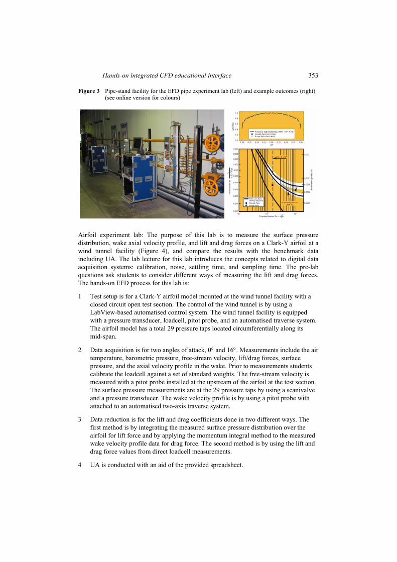
Pipe experiment lab: the purpose of this lab is to provide hands-on experience using a pipe-stand test facility (Figure 3) and modern measurement systems including pressure transducers, pitot probes, and computerised data acquisition with LabView software, to measure flow rate, velocity profiles, and friction factors in smooth and rough pipes, determining measurement uncertainties, and comparing results with benchmark data. The lecture for this lab emphasises the differences between the manual and automatised data acquisition methods and introduces the LabView software. The pre-lab questions are focused on choosing suitable measurement devices for different measurement variables. The hands-on lab exercise for this lab is as following:
1 Test setup is at the pipe-stand that is equipped with pressure taps, a Venturi-meter, and a pitot probe.
2 Data acquisition includes the measurements of static pressure, flow rate, and velocity profile for smooth or rough pipes. The pressure measurements are done in two ways: the first method is manual readings of the manometers whereas the second method is by using a pressure transducer with an automated data acquisition system.
3 Data reduction is for flow Reynolds number, friction factor, and velocity distribution, and the flow rate.
4 For UA, a spreadsheet is provided to help students with the UA procedures. The automated data acquisition system considerably facilitates the repeat measurements that are required for the precision limit estimation of the UA.
5 Students compare friction factor values from their own measurements with the Moody diagram readings from a textbook, and the velocity distribution and flow rate with the benchmark data provided by the instructors.
6 Students report measurement results and the associated uncertainty interval estimations and discuss the agreement with the benchmark data.
Hands-on integrated CFD educational interface 353
Figure 3 Pipe-stand facility for the EFD pipe experiment lab (left) and example outcomes (right) (see online version for colours)
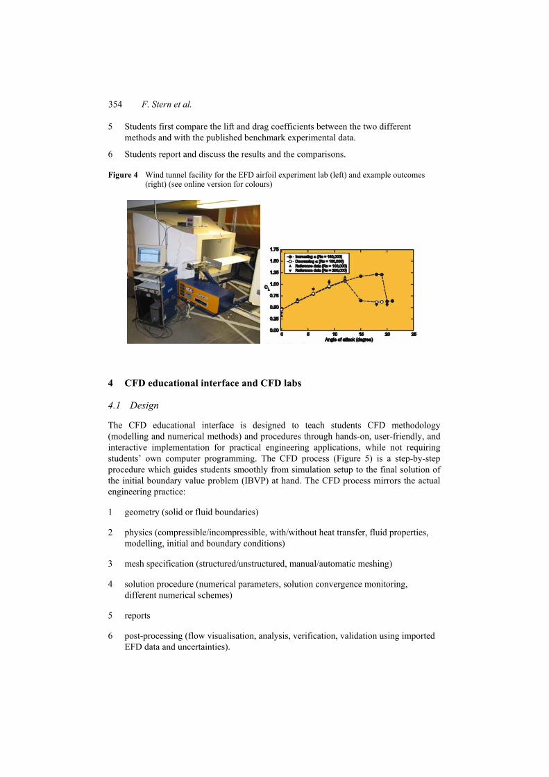
Airfoil experiment lab: The purpose of this lab is to measure the surface pressure distribution, wake axial velocity profile, and lift and drag forces on a Clark-Y airfoil at a wind tunnel facility (Figure 4), and compare the results with the benchmark data including UA. The lab lecture for this lab introduces the concepts related to digital data acquisition systems: calibration, noise, settling time, and sampling time. The pre-lab questions ask students to consider different ways of measuring the lift and drag forces. The hands-on EFD process for this lab is:
1 Test setup is for a Clark-Y airfoil model mounted at the wind tunnel facility with a closed circuit open test section. The control of the wind tunnel is by using a LabView-based automatised control system. The wind tunnel facility is equipped with a pressure transducer, loadcell, pitot probe, and an automatised traverse system. The airfoil model has a total 29 pressure taps located circumferentially along its mid-span.
2 Data acquisition is for two angles of attack, 0° and 16°. Measurements include the air temperature, barometric pressure, free-stream velocity, lift/drag forces, surface pressure, and the axial velocity profile in the wake. Prior to measurements students calibrate the loadcell against a set of standard weights. The free-stream velocity is measured with a pitot probe installed at the upstream of the airfoil at the test section. The surface pressure measurements are at the 29 pressure taps by using a scanivalve and a pressure transducer. The wake velocity profile is by using a pitot probe with attached to an automatised two-axis traverse system.
3 Data reduction is for the lift and drag coefficients done in two different ways. The first method is by integrating the measured surface pressure distribution over the airfoil for lift force and by applying the momentum integral method to the measured wake velocity profile data for drag force. The second method is by using the lift and drag force values from direct loadcell measurements.
4 UA is conducted with an aid of the provided spreadsheet.
354 F. Stern et al.
5 Students first compare the lift and drag coefficients between the two different methods and with the published benchmark experimental data.
6 Students report and discuss the results and the comparisons.
Figure 4 Wind tunnel facility for the EFD airfoil experiment lab (left) and example outcomes (right) (see online version for colours)
4 CFD educational interface and CFD labs
4.1 Design
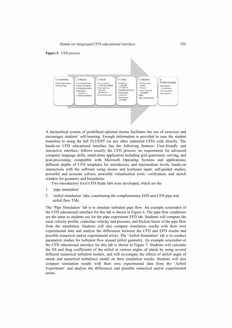
The CFD educational interface is designed to teach students CFD methodology (modelling and numerical methods) and procedures through hands-on, user-friendly, and interactive implementation for practical engineering applications, while not requiring students’ own computer programming. The CFD process (Figure 5) is a step-by-step procedure which guides students smoothly from simulation setup to the final solution of the initial boundary value problem (IBVP) at hand. The CFD process mirrors the actual engineering practice:
1 geometry (solid or fluid boundaries)
2 physics (compressible/incompressible, with/without heat transfer, fluid properties, modelling, initial and boundary conditions)
3 mesh specification (structured/unstructured, manual/automatic meshing)
4 solution procedure (numerical parameters, solution convergence monitoring, different numerical schemes)
5 reports
6 post-processing (flow visualisation, analysis, verification, validation using imported EFD data and uncertainties).
Hands-on integrated CFD educational interface 355
Figure 5 CFD process
A hierarchical system of predefined optional menus facilitates the use of exercises and encourages students’ self-learning. Enough information is provided to ease the student transition to using the full FLUENT (or any other industrial CFD) code directly. The hands-on CFD educational interface has the following features: User-friendly and interactive interface; follows exactly the CFD process; no requirement for advanced computer language skills; stand-alone application including grid generation, solving, and post-processing; compatible with Microsoft Operating Systems and applications; different depths of CFD templates for introductory and intermediate levels; hands-on interactions with the software using mouse and keyboard input; self-guided studies; powerful and accurate solvers; powerful virtualisation tools; verification; and sketch window for geometry and boundaries.
Two introductory level CFD fluids labs were developed, which are the 1 ‘pipe simulation’ 2 ‘airfoil simulation’ labs, constituting the complementary EFD and CFD pipe and
airfoil flow TMs.
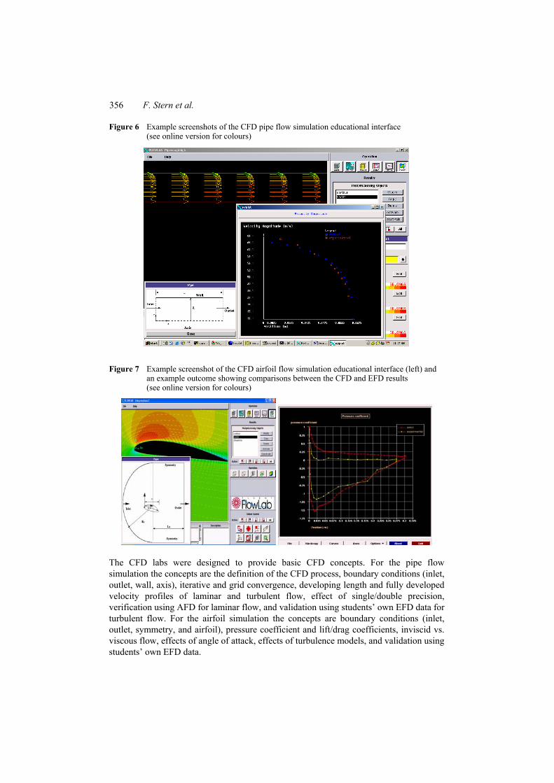
The ‘Pipe Simulation’ lab is to simulate turbulent pipe flow. An example screenshot of the CFD educational interface for this lab is shown in Figure 6. The pipe flow conditions are the same as students use for the pipe experiment EFD lab. Students will compute the axial velocity profile, centreline velocity and pressure, and friction factor of the pipe flow from the simulation. Students will also compare simulation results with their own experimental data and analyse the differences between the CFD and EFD results and possible numerical and/or experimental errors. The ‘Airfoil Simulation’ lab is to conduct parametric studies for turbulent flow around airfoil geometry. An example screenshot of the CFD educational interface for this lab is shown in Figure 7. Students will calculate the lift and drag coefficients of the airfoil at various angles of attack by using several different numerical turbulent models, and will investigate the effects of airfoil angle of attack and numerical turbulence model on their simulation results. Students will also compare simulation results with their own experimental data from the ‘Airfoil Experiment’ and analyse the differences and possible numerical and/or experimental errors.
356 F. Stern et al.
Figure 6 Example screenshots of the CFD pipe flow simulation educational interface (see online version for colours)
Figure 7 Example screenshot of the CFD airfoil flow simulation educational interface (left) and an example outcome showing comparisons between the CFD and EFD results (see online version for colours)
The CFD labs were designed to provide basic CFD concepts. For the pipe flow simulation the concepts are the definition of the CFD process, boundary conditions (inlet, outlet, wall, axis), iterative and grid convergence, developing length and fully developed velocity profiles of laminar and turbulent flow, effect of single/double precision, verification using AFD for laminar flow, and validation using students’ own EFD data for turbulent flow. For the airfoil simulation the concepts are boundary conditions (inlet, outlet, symmetry, and airfoil), pressure coefficient and lift/drag coefficients, inviscid vs. viscous flow, effects of angle of attack, effects of turbulence models, and validation using students’ own EFD data.

Hands-on integrated CFD educational interface 357
Table 5 CFD labs learning objectives and evaluation
Qua
ntita
tive
data
on
stud
ent p
erfo
rman
ce
(on
a sc
ale
of 1
0)
Obj
ectiv
es
Asse
ssm
ent
tech
niqu
e ’0
2 ’0
3 ’0
4 ’0
5 ’0
6 ’0
7 ’0
8 ’0
9 ’1
0 Av
g SD
1 Pr
ovid
e st
uden
ts w
ith ‘h
ands
-on’
ex
perie
nce
with
CFD
met
hodo
logy
(m
odel
ling
and
num
eric
al m
etho
ds)
and
proc
edur
es th
roug
h st
ep-b
y-st
ep
appr
oach
follo
win
g C
FD p
roce
ss:
geom
etry
, phy
sics
, mes
h, s
olve
, re
ports
, and
pos
t pro
cess
ing.
Surv
ey
7.8
7.3
8.4
8.7
8.5
8.4
8.6
8.0
8.0
8.2
0.5
2 H
elp
stud
ents
to le
arn
CFD
m
etho
dolo
gy a
nd p
roce
dure
s th
roug
h th
e ed
ucat
iona
l int
erfa
ce.
Surv
ey
n/a
n/a
n/a
n/a
n/a
n/a
8.4
8.4
8.1
8.3
0.2
3 St
uden
ts w
ill b
e ab
le to
app
ly C
FD
proc
ess t
hrou
gh u
se o
f edu
catio
nal
inte
rfac
e fo
r com
mer
cial
sof
twar
e to
an
alys
e pr
actic
al e
ngin
eerin
g pr
oble
ms.
Surv
ey
8.0
7.5
8.4
8.6
8.6
8.6
8.1
8.2
8.0
8.2
0.4
4 St
uden
ts w
ill b
e ab
le to
con
duct
nu
mer
ical
unc
erta
inty
ana
lysi
s thr
ough
ite
rativ
e an
d gr
id c
onve
rgen
ce s
tudi
es.
Surv
ey
7.8
7.4
8.1
8.1
8.2
8.0
8.2
8.2
7.9
8.0
0.3
5 St
uden
ts w
ill b
e ab
le to
val
idat
e th
eir
com
puta
tion
resu
lts w
ith E
FD d
ata
from
thei
r com
plem
enta
ry
expe
rimen
tal l
abor
ator
y.
Surv
ey
7.6
7.5
8.4
8.7
8.3
8.4
8.1
8.3
8.0
8.1
0.4
358 F. Stern et al.
Table 5 CFD labs learning objectives and evaluation (continued)
Qua
ntita
tive
data
on
stud
ent p
erfo
rman
ce
(on
a sc
ale
of 1
0)
Obj
ectiv
es
Asse
ssm
ent
tech
niqu
e ’0
2 ’0
3 ’0
4 ’0
5 ’0
6 ’0
7 ’0
8 ’0
9 ’1
0 A
vg
SD
Stud
ents
will
be
able
to
setu
p I
BV
P
thro
ugh
the
educ
atio
nal i
nter
face
, in
clud
ing:
Surv
ey
n/a
8.1
8.4
8.1
8.2
0.2
1 cr
eate
geo
met
ry
2 se
tup
flui
d p
rope
rtie
s 3
gene
rate
mes
h au
tom
atic
ally
or
man
ually
4
setu
p ap
pro
pria
te s
olve
rs
5 re
por
t
6
6 p
ost-
pro
cess
sim
ulat
ion
data
.
n/a
n/a
n/a
n/a
n/a
7 St
uden
ts w
ill b
e ab
le t
o le
arn
mor
e fl
ow p
hysi
cs b
eyon
d th
e co
ndit
ions
th
ey u
sed
in t
he c
omp
lem
enta
ry E
FD
la
bs. S
tude
nts
will
con
duct
par
amet
ric
stud
ies
usin
g th
e ed
ucat
iona
l int
erfa
ce
to in
vest
igat
e in
visc
id v
s. v
isco
us
flow
s, e
ffec
t of
tur
bule
nt m
odel
s,
effe
ct o
f an
gles
of
atta
ck, a
nd e
ffec
t of
orde
r of
acc
urac
ies,
etc
.
Surv
ey
n/a
n/a
n/a
n/a
n/a
n/a
8.1
8.3
8.1
8.2
0.1
8 St
uden
ts w
ill b
e ab
le to
ana
lyse
and
re
late
CF
D re
sults
to
fluid
phy
sics
and
cl
assr
oom
lect
ures
, inc
ludi
ng
team
wor
k an
d p
rese
ntat
ion
of re
sults
in
wri
tten
and
gra
phic
al f
orm
.
Surv
ey
7.5
7.1
8.0
8.2
8.0
8.0
8.3
8.3
8.1
7.9
0.4
Lab
rep
ort 1
n/
a n/
a n/
a 9.
5 9.
2 9.
3 9.
0 9.
0 9.
1 9.
2 0.
2 L
ab r
epor
t 2
n/a
n/a
n/a
9.6
9.6
9.5
9.5
9.4
9.4
9.5
0.1
Pre-
test
n/
a n/
a n/
a 5.
7 5.
7 5.
2 4.
9 5.
1 4.
9 5.
2 0.
4 (C
onfi
denc
e)
n/a
n/a
n/a
n/a
n/a
n/a
n/a
(3.3
) (3
.3)
(3.3
)
Pos
t-te
st
n/a
n/a
n/a
7.0
6.6
6.9
7.3
8.1
6.7
7.1
0.5
Con
fide
nce
n/a
n/a
n/a
n/a
n/a
n/a
n/a
(8.0
) (6
.7)
(7.3
)
Goa
ls 1
to 8
Scor
e in
crea
se
n/a
n/a
n/a
1.4
0.9
1.6
2.4
3.0
1.8
1.9
0.7

Hands-on integrated CFD educational interface 359
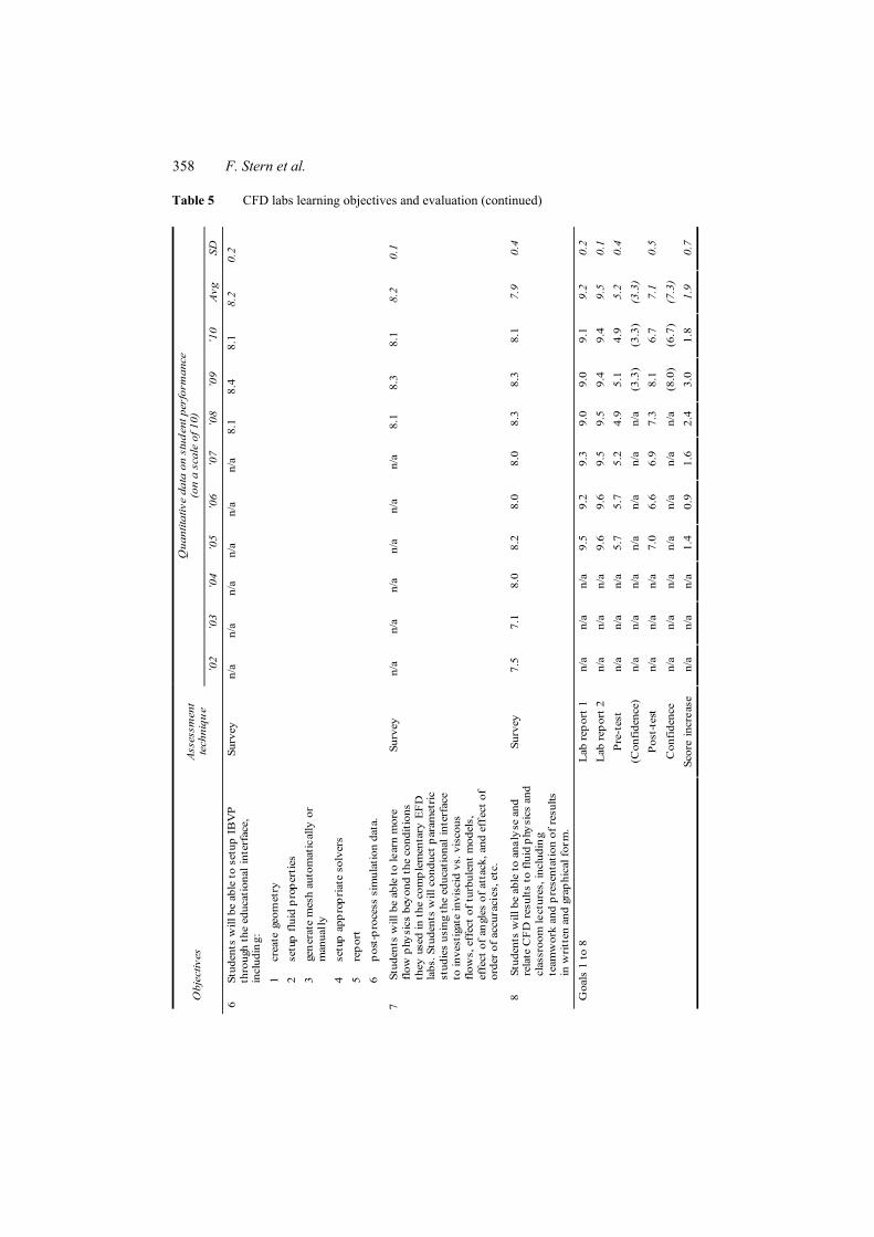
4.2 CFD learning objectives
The learning objectives of the CFD labs are listed in Table 5. Eight objectives were developed based on the lab concepts (Table 1) covering the CFD process, verification and validation, flow physics, and relationship to the classroom lectures and EFD labs. The lab reports, pre/post-test and end-of-the semester survey are used for assessment.
4.3 Implementation
Prior to the beginning of the two CFD labs, one classroom lecture is given presenting the CFD methodology and procedures in general. The CFD lectures cover what, why, and where is CFD used; modelling; numerical methods; types of CFD codes; the CFD process; an example; and an introduction to the CFD educational interface and student applications. For each CFD labs, detailed exercise notes guide students step-by-step on how to use the educational interface to achieve specific objectives for each lab, including how to input/output data, what figures/data need to be saved for the lab report, and questions that need to be answered in the lab report. CFD lab report instructions guide students step-by-step through how to present their results and findings in written and graphical form. Lectures and exercise notes are distributed through the class website. The CFD Lab report covers the purpose and design of the simulation, the CFD process, data analysis and discussion, and conclusion.
Students’ hands-on simulation procedures for the CFD labs follow the ‘CFD process’:
1 Geometry: students can create various geometries and domains including pipe and airfoil. Students need to input different parameters for the particular class of geometry they have selected, such as pipe radius and length and airfoil ‘O’/’C’ mesh topology, chord length, angle of attack.
2 Physics: students need to choose whether to model the flow as compressible/incompressible, with/without heat transfer, as inviscid/viscous, and as laminar/turbulent; set up the fluid properties (density, viscosity, specific heat, thermal conductivity); select appropriate turbulence models, if appropriate; and define boundary conditions (inlet, outlet, symmetry, wall, axis) and initial conditions.
3 Mesh: both structured and unstructured meshes are available. When using structured meshes the student either automatically or manually generates the desired meshes. Automatic meshing is designed for novice/introductory level students. By specifying ‘coarse,’ ‘medium,’ or ‘fine’ meshes, the educational interface will automatically generate a mesh of the corresponding grid density using parameters hard-coded in the software. Manual meshing is designed for intermediate/professional level students.
4 Solve: students need to specify appropriate solution parameters. These include whether the flow is to be treated as steady or unsteady, maximum iteration count, convergence limit, numerical precision (single/double), numerical differentiation scheme (1st order, 2nd order, QUICK scheme), and axial output locations (for output variables to compare with EFD).
360 F. Stern et al.
5 Reports: after the iterative solution process converges, all the integral parameters of the solution, such as total forces and lift/drag coefficients, are reported. Various XY plots and verification and validation functions are also available for students to validate their simulations using benchmark, or their own, EFD data, and to conduct CFD UA. The total reduction in magnitude of solution residual and the final level of solution residual are used to determine stopping criteria for the iterative solution process. For unsteady flows, the time history of integral variables (e.g., drag force) is used to determine the degree of convergence of the iterative solution. Grid uncertainty is analysed using two meshes generated by the automatic function of the interface (coarse and medium, or coarse and fine). Grid refinement ratio can also be used to create different sets of meshes.
6 Post-processing: powerful tools can be used to visualise and examine the flow field, such as contours (total/static pressure, velocities, turbulent kinetic energy, temperature, Mach number), vectors, streamlines, and animations.
5 ePIV/Flowcoach laboratory
5.1 Design
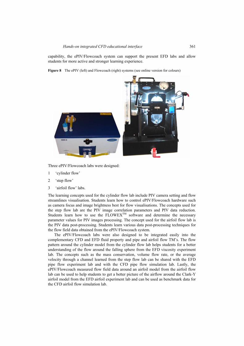
The ePIV and Flowcoach systems (Figure 8) are educational versions of the particle image velocimetry (PIV) for flow visualisations and measurements, developed by the Interactive Flow Studies Corporation (http://www.interactiveflows.com/). PIV is a widely used image-based flow field measurement method and has become a very powerful technique for studying fluid mechanics. In general, a PIV system consists of a number of scientific digital cameras and class-IV level high-powered lasers, which are usually expensive and classified as hazardous, thus may not be affordable or adequate for general educational use at typical classrooms or laboratories. In contrast, the ePIV or the Flowcoach system is compact-sized, low-cost, and safe for use, intended to be used as an educational tool. The ePIV consists of a digital camera (600 × 480 pixels with 30 fps), a small laser (class-III, 15 mW green continuous diode), an optical lens, a small water pump, a seed water reservoir, and a small water channel module, which are all secured and covered in a small box housing. Various shaped flow model-inserts (25 mm × 30 mm) are easily replaceable inside the water channel module. The inserts can be made with a rapid prototyping system, can be machined from metal or acrylic, or can be moulded. The Flowcoach system is the 2nd generation of the ePIV system. The Flowcoach system consists of similar components as the ePIV system, but an open system without a cover or a housing. The Flowcoach system uses an LED illumination instead of a laser and bigger size flow model-inserts (80 mm × 80 mm). The ePIV system is for laminar flows only whereas it is possible to visualise laminar, transition and turbulent flows (up to Re = 25,000) with the Flowcoach system. A higher resolution and faster speed camera can be mounted on Flowcoach which will allow PIV analysis of turbulent flows. Both ePIV and Flowcoach systems use the FLOWEXTM software (http://demo.interactiveflows.com/) for camera control, image acquisition, and PIV analysis. The FLOWEXTM’s internet access capability was used for remote diagnostic purposes with the Interactive Flow Studies. By virtue of its strong flow visualisation
Hands-on integrated CFD educational interface 361
capability, the ePIV/Flowcoach system can support the present EFD labs and allow students for more active and stronger learning experience.
Figure 8 The ePIV (left) and Flowcoach (right) systems (see online version for colours)
Three ePIV/Flowcoach labs were designed:
1 ‘cylinder flow’
2 ‘step flow’
3 ‘airfoil flow’ labs.
The learning concepts used for the cylinder flow lab include PIV camera setting and flow streamlines visualisation. Students learn how to control ePIV/Flowcoach hardware such as camera focus and image brightness best for flow visualisations. The concepts used for the step flow lab are the PIV image correlation parameters and PIV data reduction. Students learn how to use the FLOWEXTM software and determine the necessary parameter values for PIV images processing. The concept used for the airfoil flow lab is the PIV data post-processing. Students learn various data post-processing techniques for the flow field data obtained from the ePIV/Flowcoach system.
The ePIV/Flowcoach labs were also designed to be integrated easily into the complementary CFD and EFD fluid property and pipe and airfoil flow TM’s. The flow pattern around the cylinder model from the cylinder flow lab helps students for a better understanding of the flow around the falling sphere from the EFD viscosity experiment lab. The concepts such as the mass conservation, volume flow rate, or the average velocity through a channel learned from the step flow lab can be shared with the EFD pipe flow experiment lab and with the CFD pipe flow simulation lab. Lastly, the ePIV/Flowcoach measured flow field data around an airfoil model from the airfoil flow lab can be used to help students to get a better picture of the airflow around the Clark-Y airfoil model from the EFD airfoil experiment lab and can be used as benchmark data for the CFD airfoil flow simulation lab.

362 F. Stern et al.
5.2 ePIV/Flowcoach learning objectives
The learning objectives of ePIV/Flowcoach labs are listed in Table 6. Two objectives were developed based on the lab concepts (Table 1) to cover the principles and applications of the PIV technique and to help students understand the fundamental fluid dynamics concepts better with the aid of flow visualisation. The lab reports, pre/post-test and end-of-the semester survey are used for assessment. Table 6 ePIV/Flowcoach labs learning objectives and evaluation
Quantitative data on student performance (on a scale of 10) Objectives Assessment
technique ’02 ’03 ’04 ’05 ’06 ’07 ’08 ’09 ’10 Avg SD
Pre-test n/a n/a n/a n/a n/a n/a 6.8 3.8 3.7 4.8 1.8
(Confidence) n/a n/a n/a n/a n/a n/a (5.0) (3.0) (3.0) (3.7) (1.2)
Post-test n/a n/a n/a n/a n/a n/a 8.5 7.5 5.9 7.3 1.3
(Confidence) n/a n/a n/a n/a n/a n/a (8.0) (7.7) (6.7) (7.3) (0.7)
1 Provide students with ‘hands-on’ experience on the PIV flow visualisation and flow field measurement technique following the ‘EFD process’ to understand the principles and applications of the PIV technique.
2 Students will be able to understand fundamental fluid dynamics concepts better with the aid of flow visualisation.
Score increase
n/a n/a n/a n/a n/a n/a 1.7 3.7 2.2 2.5 1.0
5.3 Implementation
The ePIV/Flowcoach labs are given during the EFD lab meeting hours. Typically two student groups attend the lab meetings and each group begins with either ePIV/Flowcoach lab or EFD lab then switches. The ePIV/Flowcoach labs also share the TM with the EFD labs. However, separate data reduction sheets or supplementary materials for the ePIV/Flowcoach labs as necessary. The hands-on experiment procedures for ePIV/Flowcoach labs follow the ‘EFD Process’ similar to EFD labs; however the UA step of the ‘EFD Process’ has not been implemented yet for the ePIV/Flowcoach labs.
Cylinder flow lab: the purpose of this lab is to visualise the flow around a circular cylinder model and to estimate the flow Reynolds number by comparing the flow streamline patterns from the visualisation with the published flow images tested at various flow conditions. Students also learn about the flow patterns around bluff bodies during this lab. For test setup, the ePIV/Flowcoach system is fitted with a circular cylinder model. By using the FLOWEXTM, students first adjust the focus of camera and change camera control parameters such as brightness, exposure, and gain to achieve optimal flow streamlines visualisation. Once obtained the desired camera parameters, flow speed is adjusted over a range to observe how the flow streamlines pattern changes, especially at the wake region behind the cylinder. Students compare the streamlines from the ePIV/Flowcoach images with the provided sample images as guidelines and estimate

Hands-on integrated CFD educational interface 363
the Reynolds number of the flow. Streamline images are captured for different Reynolds number cases ranging between approximately 2 and 90 according to the flow speed. Students report two ePIV/Flowcoach streamline images with specified the camera settings used for image capture, qualitative sketches of the streamlines, and the estimated Reynolds numbers for a low and high Reynolds numbers. Students are asked to explain the different flow patterns between the low and high Reynolds numbers, based on their ePIV/Flowcoach flow observations. A typical example of the Flowcoach streamline image is shown in Figure 9.
Figure 9 Streamlines visualisation around a cylinder model for the ePIV/Flowcoach cylinder flow lab (top) and a conceptual sketch of the streamlines from a textbook (bottom) (see online version for colours)
Step flow lab: the purpose of this lab is to measure the velocity field of the flow over a step-up model and determine the volume flow rate and cross-sectional average velocity of the flow. During this lab students learn about the fluid dynamics concepts such as the mass conservation law and the continuity equation. The PIV particle images from the ePIV/Flowcoach are processed for flow velocity vectors by using the FLOWEXTM software. For this, three PIV parameters can be adjusted including interrogation window size, shift size, and PIV pairs. The interrogation window size parameter sets the size of the PIV interrogation window in pixels. The shift size parameter determines the pixel distance that the software moves to start a new interrogation window. The PIV pairs parameter specifies how many pairs of images are used for PIV calculations. Results computed for each individual pair are averaged together, reducing precision error. Data reduction for ePIV includes the following steps: calculates the average velocity and flow rate for every x-value in the recorded data. Plot the calculated average velocities and flow rates versus x-position. Examples of the plots are shown in Figure 10. Students report plots of average velocity and flow rate versus x-position and answer to the questions about such as the effect of the cross-sectional area of the channel on the average velocity and the flow rate.
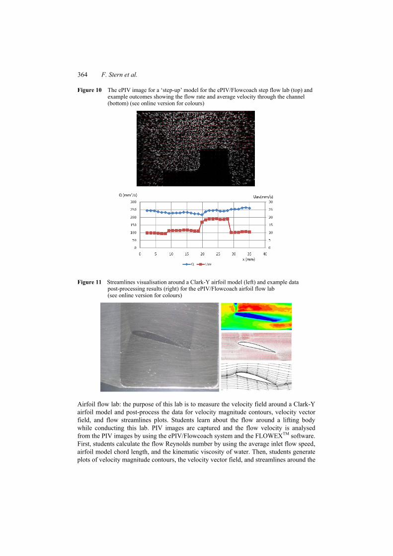
364 F. Stern et al.
Figure 10 The ePIV image for a ‘step-up’ model for the ePIV/Flowcoach step flow lab (top) and example outcomes showing the flow rate and average velocity through the channel (bottom) (see online version for colours)
Figure 11 Streamlines visualisation around a Clark-Y airfoil model (left) and example data post-processing results (right) for the ePIV/Flowcoach airfoil flow lab (see online version for colours)
Airfoil flow lab: the purpose of this lab is to measure the velocity field around a Clark-Y airfoil model and post-process the data for velocity magnitude contours, velocity vector field, and flow streamlines plots. Students learn about the flow around a lifting body while conducting this lab. PIV images are captured and the flow velocity is analysed from the PIV images by using the ePIV/Flowcoach system and the FLOWEXTM software. First, students calculate the flow Reynolds number by using the average inlet flow speed, airfoil model chord length, and the kinematic viscosity of water. Then, students generate plots of velocity magnitude contours, the velocity vector field, and streamlines around the

Hands-on integrated CFD educational interface 365
airfoil for both 0º and 16º angles of attack by using commercial graphic software (e.g., Tecplot®). Examples of the plots are shown in Figure 11. Students report the flow Reynolds number and the plots and answer to the questions about such as the effect of angle of attack of the airfoil model on the flow pattern and separation.
6 Evaluation and assessment
The course and lab evaluation is based on student performance metrics in homework, quizzes, exams, lab reports and pre/post-tests along with an end-of-semester survey. The course and problem solving, CFD lab and EFD lab objectives were developed during the ISTUE project in collaboration with CEA, as shown in Tables 2 to 5. Recently ePIV/Flowcoach objectives were developed, again in collaboration CEA, as shown in Table 6. The pre/post-test and end-of-semester survey items were also developed in collaboration CEA. The student performance metrics and end-of-semester survey items are cross-references to the objectives, as shown in Tables 2 to 6. Data have been collected over the last nine years.
The pre/post-test consists of two forms (forms A and B) which are designed to be parallel. All test items are objectively-scoreable with a format of either multiple-choice or true-false or supply-type. Students are randomly assigned to take either form A or form B as a pre-test at the beginning of the semester. At the end of the semester, all students take a post-test, which include both sets of items from forms A and B. Thus, on the post-test, students respond to one set of items they had previously seen on the pre-test and an additional set of items that they had never seen before. In addition to responding to individual items, students are asked to rate their confidence in their response to each individual item. Confidence is rated on a four-point scale ranging from ‘Just Guessing’ (scored as 0) to ‘Completely Confident’ (scored as 3). On the CFD assessment, forms A and B each contains 11 items, ten of which are unique and one of which appears on both forms A and B. Thus, the CFD post-test includes 21 items. On the EFD assessment, forms A and B each contains 12 unique items. Thus, the EFD post-test includes 24 items. Finally, on the ePIV/Flowcoach assessment, forms A and B each contains six unique items. Thus, the ePIV post-test includes 12 items.
The end-of-semester survey items were developed for course general (8 items for 8 objectives), problem solving (27 items for 7 objectives), CFD labs (15 items for 8 objectives), and EFD labs (13 items for 5 objectives); total 62 items for 28 objectives. Note that one survey item was used for both CFD and EFD labs. Note also that two items for EFD labs are related to ePIV/Flowcoach labs. Students responded to survey items by using a six-point Likert type scale ranging from ‘Strongly agree’ (scored as 6) to ‘Strongly disagree’ (scored as 1). Respondents with insufficient information or who do not want to respond can choose a ‘No opinion’ respond.
Table 7 provides a summary of the evaluation. Presented in the summary are the time-average mean and standard deviations (SD) for the student performance metrics and end-of-semester survey items. It is noted that all of the assessment results were rescaled by using a ten-point scale for direct comparisons between different assessment techniques. The resulting scores can be interpreted to mean the number of items correct out of ten, as stepped up or stepped down depending on the total number of actual items on the assessment.
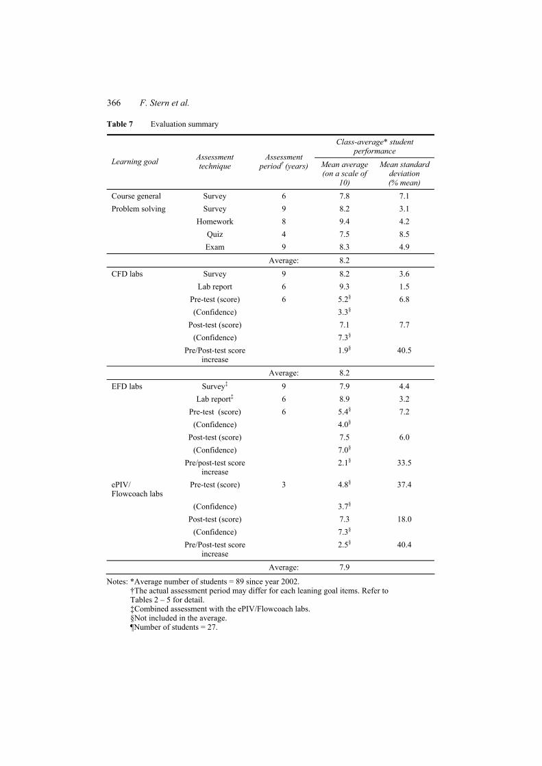
366 F. Stern et al.
Table 7 Evaluation summary
Class-average* student performance
Learning goal Assessment technique
Assessment period† (years) Mean average
(on a scale of 10)
Mean standard deviation (% mean)
Course general Survey 6 7.8 7.1 Problem solving Survey 9 8.2 3.1 Homework 8 9.4 4.2 Quiz 4 7.5 8.5 Exam 9 8.3 4.9
Average: 8.2
CFD labs Survey 9 8.2 3.6 Lab report 6 9.3 1.5 Pre-test (score) 6 5.2§ 6.8 (Confidence) 3.3§ Post-test (score) 7.1 7.7 (Confidence) 7.3§
Pre/Post-test score increase
1.9§ 40.5
Average: 8.2
EFD labs Survey‡ 9 7.9 4.4 Lab report‡ 6 8.9 3.2 Pre-test (score) 6 5.4§ 7.2 (Confidence) 4.0§ Post-test (score) 7.5 6.0 (Confidence) 7.0§
Pre/post-test score increase
2.1§ 33.5
ePIV/ Flowcoach labs
Pre-test (score) 3 4.8§ 37.4
(Confidence) 3.7§ Post-test (score) 7.3 18.0 (Confidence) 7.3§
Pre/Post-test score increase
2.5§ 40.4
Average: 7.9
Notes: *Average number of students = 89 since year 2002. †The actual assessment period may differ for each leaning goal items. Refer to Tables 2 – 5 for detail. ‡Combined assessment with the ePIV/Flowcoach labs. §Not included in the average. ¶Number of students = 27.
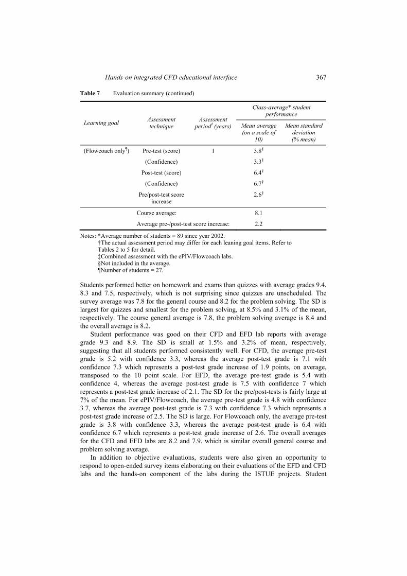
Hands-on integrated CFD educational interface 367
Table 7 Evaluation summary (continued)
Class-average* student performance
Learning goal Assessment technique
Assessment period† (years) Mean average
(on a scale of 10)
Mean standard deviation (% mean)
(Flowcoach only¶) Pre-test (score) 1 3.8§
(Confidence) 3.3§
Post-test (score) 6.4§
(Confidence) 6.7§
Pre/post-test score increase
2.6§
Course average: 8.1
Average pre-/post-test score increase: 2.2
Notes: *Average number of students = 89 since year 2002. †The actual assessment period may differ for each leaning goal items. Refer to Tables 2 to 5 for detail. ‡Combined assessment with the ePIV/Flowcoach labs. §Not included in the average. ¶Number of students = 27.
Students performed better on homework and exams than quizzes with average grades 9.4, 8.3 and 7.5, respectively, which is not surprising since quizzes are unscheduled. The survey average was 7.8 for the general course and 8.2 for the problem solving. The SD is largest for quizzes and smallest for the problem solving, at 8.5% and 3.1% of the mean, respectively. The course general average is 7.8, the problem solving average is 8.4 and the overall average is 8.2.
Student performance was good on their CFD and EFD lab reports with average grade 9.3 and 8.9. The SD is small at 1.5% and 3.2% of mean, respectively, suggesting that all students performed consistently well. For CFD, the average pre-test grade is 5.2 with confidence 3.3, whereas the average post-test grade is 7.1 with confidence 7.3 which represents a post-test grade increase of 1.9 points, on average, transposed to the 10 point scale. For EFD, the average pre-test grade is 5.4 with confidence 4, whereas the average post-test grade is 7.5 with confidence 7 which represents a post-test grade increase of 2.1. The SD for the pre/post-tests is fairly large at 7% of the mean. For ePIV/Flowcoach, the average pre-test grade is 4.8 with confidence 3.7, whereas the average post-test grade is 7.3 with confidence 7.3 which represents a post-test grade increase of 2.5. The SD is large. For Flowcoach only, the average pre-test grade is 3.8 with confidence 3.3, whereas the average post-test grade is 6.4 with confidence 6.7 which represents a post-test grade increase of 2.6. The overall averages for the CFD and EFD labs are 8.2 and 7.9, which is similar overall general course and problem solving average.
In addition to objective evaluations, students were also given an opportunity to respond to open-ended survey items elaborating on their evaluations of the EFD and CFD labs and the hands-on component of the labs during the ISTUE projects. Student

368 F. Stern et al.
comments on the survey questions, for example, “Evaluate the hands-on aspects of this course …” or “What were the best features of the EFD/CFD lab and what worked especially well for you?”, were grouped into a few categories and summarised in Stern et al. (2004a) for EFD labs and in Stern et al. (2004b) for CFD labs. In general students were more positive on the CFD labs appreciating the value of visualisation of CFD results and the ease of use of the CFD educational interface. At the same time students also suggested a number of improvements on the labs, for example, requesting more instructions on CFD modelling or on using the educational interface including manual mesh generation. For EFD labs, students commented that the hands-on aspect of the labs helped them learn, but many of the students commented that they needed more opportunity to learn or to be more involved in the test design and setup.
For ePIV/Flowcoach labs, students were asked to address their comments and suggestions on the labs at the conclusion part of lab reports during the time span 2008 to 2010. Students were mostly positive on the ePIV/Flowcoach labs. They felt that the labs were enjoyable and useful to understand fluids dynamics better, especially from the flow visualisation aspect of the ePIV and Flowcoach systems. However, students also suggested that the labs could be more comprehensive than the current lab implementations. It was remarked that most of the students, either positive or negative, wanted more hands-on experience with the labs.
Just as with previous studies of EFD and CFD conducted by Stern et al. (2006), pre-tests and post-tests were used to investigate students’ ePIV and ePIV/Flowcoach outcomes. Tables 8 and 9 present more details about students’ learning of the content. Table 8 reports the ePIV pre-test mean scores, mean ‘Same Form’ post-test composite scores and mean ‘Parallel Form’ post-test composite scores for students randomly assigned to take form A or form B as the pre-test. Although form A pre-test mean scores were slightly higher than form B pre-test mean scores (indicating form B was slightly more difficult), the similarity in mean scores suggests that differences in form difficulty were not substantial. Gain scores from pre- to post-test were highly significant. Pre-test mean scores represented roughly 45% and 30% of the maximum possible points respectively for forms A and B, whereas post-test mean scores (across both forms) constituted approximately 74% of the maximum possible points (six items). Thus, both groups of students demonstrated both practically and statistically significant growth in their mastery of course content during the fall semester, 2009. It should be noted that despite robust evidence of student growth, student scores on the pre-test indicate that incoming students were able to get a fair number of items correct prior to instruction.
Table 8 ePIV pre- and post-test mean composite scores by form assignment for 2009
Pre-test form N Pre-test mean (SD) Same form post-test mean (SD)
Parallel form post-test mean (SD)
2.67 4.82* 4.26* Form A 49
(1.36) (0.95) (0.91)
1.88 3.94* 4.86* Form B 51
(1.27) (0.99) (0.96)
Note: *Indicates improvement is significant from pre- to post-test at the p < .0001 level.
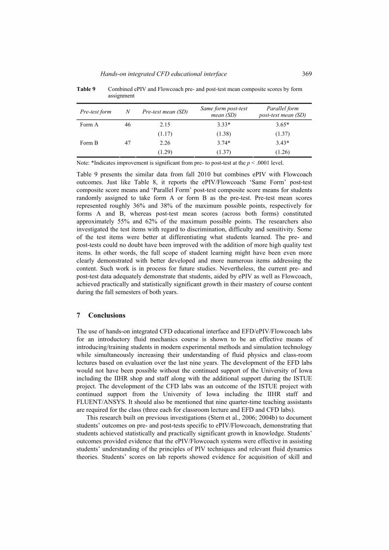
Hands-on integrated CFD educational interface 369
Table 9 Combined ePIV and Flowcoach pre- and post-test mean composite scores by form assignment
Pre-test form N Pre-test mean (SD) Same form post-test mean (SD)
Parallel form post-test mean (SD)
2.15 3.33* 3.65* Form A 46 (1.17) (1.38) (1.37) 2.26 3.74* 3.43* Form B 47
(1.29) (1.37) (1.26)
Note: *Indicates improvement is significant from pre- to post-test at the p < .0001 level.
Table 9 presents the similar data from fall 2010 but combines ePIV with Flowcoach outcomes. Just like Table 8, it reports the ePIV/Flowcoach ‘Same Form’ post-test composite score means and ‘Parallel Form’ post-test composite score means for students randomly assigned to take form A or form B as the pre-test. Pre-test mean scores represented roughly 36% and 38% of the maximum possible points, respectively for forms A and B, whereas post-test mean scores (across both forms) constituted approximately 55% and 62% of the maximum possible points. The researchers also investigated the test items with regard to discrimination, difficulty and sensitivity. Some of the test items were better at differentiating what students learned. The pre- and post-tests could no doubt have been improved with the addition of more high quality test items. In other words, the full scope of student learning might have been even more clearly demonstrated with better developed and more numerous items addressing the content. Such work is in process for future studies. Nevertheless, the current pre- and post-test data adequately demonstrate that students, aided by ePIV as well as Flowcoach, achieved practically and statistically significant growth in their mastery of course content during the fall semesters of both years.
7 Conclusions
The use of hands-on integrated CFD educational interface and EFD/ePIV/Flowcoach labs for an introductory fluid mechanics course is shown to be an effective means of introducing/training students in modern experimental methods and simulation technology while simultaneously increasing their understanding of fluid physics and class-room lectures based on evaluation over the last nine years. The development of the EFD labs would not have been possible without the continued support of the University of Iowa including the IIHR shop and staff along with the additional support during the ISTUE project. The development of the CFD labs was an outcome of the ISTUE project with continued support from the University of Iowa including the IIHR staff and FLUENT/ANSYS. It should also be mentioned that nine quarter-time teaching assistants are required for the class (three each for classroom lecture and EFD and CFD labs).
This research built on previous investigations (Stern et al., 2006; 2004b) to document students’ outcomes on pre- and post-tests specific to ePIV/Flowcoach, demonstrating that students achieved statistically and practically significant growth in knowledge. Students’ outcomes provided evidence that the ePIV/Flowcoach systems were effective in assisting students’ understanding of the principles of PIV techniques and relevant fluid dynamics theories. Students’ scores on lab reports showed evidence for acquisition of skill and
370 F. Stern et al.
knowledge related to the overall lab implementation goals. Students’ growth between pre- and post-tests was substantial both for knowledge as measured and for their confidence ratings of that knowledge. Survey results demonstrated that as a result of the ePIV/Flowcoach labs, students could conduct experiments and analyse the ePIV/Flowcoach results to gain increased understanding of fluid physics.
Sustaining and further developing the hands-on integrated CFD educational interface and EFD/ePIV/Flowcoach labs is a major issue. Clearly, significant institutional commitment is required especially in support of the EFD labs and teaching assistants. For the EFD labs laser Doppler and hot-wire velocimetry are planned for the pipe and airfoil experiments, respectively, to replace the current pitot probe measurement systems. For the CFD labs, the most important issue is the continued development and use of the CFD educational interface since the end of the ISTUE project. A post ISTUE project workshop was held on July 14, 2005 at IIHR, supported by NSF supplemental funding, with over 30 attendees of whom 18 were external to the ISTUE project and representing 14 different universities and the departments of bio, marine, mechanical, nuclear, food, materials science and chemical, atmospheric sciences, and civil engineering. There was widespread interest in the workshop, although limited funding precluded more attendees. The primary purpose of the workshop was to disseminate the CFD educational interface and conduct an informal assessment of the merits of the interface and the simulations developed to date. Specific objectives included:
1 evaluation of the interface by peer faculty
2 identifying needed enhancements and additional simulations
3 determining applicability by peer faculty.
The workshop agenda covered demonstration of the CFD educational interface along with its previous implementation and evaluation, followed by visiting faculty presentations and discussion of applicability to match their teaching needs. The independent evaluation conducted by the CEA indicated that faculties found the workshop valuable and verified their interests in implementing and if necessary further developing and/or adapting the CFD educational for their respective courses and laboratories. An outcome from the workshop was an NSF National Dissemination proposal, which unfortunately was not funded since CFD was considered one example of the wider field of computational science; thus, a broader scope was recommended.
Another development was that FLUENT is part of ANSYS and Flowlab is no longer generally available, but to be replaced by the current ANSYS Workbench environment. Some ISTUE faculties have already transitioned to the ANSYS Workbench, but a general purpose CFD educational interface is not yet available.
Acknowledgements
The University of Iowa and IIHR shop and staff supported the EFD and CFD labs. Shane Moeykens, Strategic Partnerships Manger, ANSYS Inc., is gratefully acknowledged for his continuing support of the use of FlowLab at the University of Iowa. The implementation of ePIV/Flowcoach was supported by NSF grant #:0844891-SBIR Phase II-Educational PIV Suites.
Hands-on integrated CFD educational interface 371
References Budny, D. and Torick, D. (2010) ‘Design of a multi-purpose experiment for use in a fluid
mechanics lab’, ASEE/IEEE Frontiers in Education Conference. Feisel, L.D. and Rosa, A.J. (2005) ‘The role of the laboratory in undergraduate engineering
education’, Journal of Engineering Education, Vol. 94, No. 1, pp.121–130. Fraser, D.M., Pillay, R., Tjatindi, L. and Case, J.M. (2007) ‘Enhancing the learning of fluid
mechanics using computer simulations’, Journal of Engineering Education, Vol. 96, No. 4, pp.381–388.
Keith, J., Fogler, H.S., Thomas, V., Chmielewski, D. and Gross, M. (2008) ‘Cache module development for introducing energy into the chemical engineering curriculum: fuel cells’, ASEE Annual Conference, 22–25 June, Pittsburgh, PA.
Okamoto, N., Hsu, T-R. and Bash, C.E. (2009) ‘A thermal management of electronics course and laboratory for undergraduates’, Advances in Engineering Education, Winter.
Sert, C. and Nakboglu, G. (2007) ‘Use of computational fluid dynamics (CFD) in teaching fluid mechanics’, ASEE Annual Conference, 25–27 June, Honolulu, HI.
Stern, F., Muste, M., Ghosh, S., Shao, J. and Yarbrough, D. (2004a) ‘Development hands-on student experience with modern facilities, measurement systems, and uncertainty analysis in undergraduate fluids engineering laboratories’, ASEE Annual Conference, 20–23 June, Salt Lake City, UT.
Stern, F., Xing, T., Yarbrough, D., Rothmayer, A., Rajagopalan, G., Otta, S.P., Caughey, D. Bhaskaran, R., Smith, S., Hutchings, B. and Moeykens, S. (2004b) ‘Development of hands-on CFD educational interface for undergraduate engineering courses and laboratories’, ASEE Annual Conference, 20–23 June, Salt Lake City, UT.
Stern, F., Xing, T., Yarbrough, D., Rothmayer, A., Rajagopalan, G., Otta, S.P., Caughey, D., Bhaskaran, R., Smith, S., Hutching, B. and Moeykens, S. (2006) ‘Hands-on CFD educational interface for engineering courses and laboratories’, Journal Engineering Education, Vol. 95, No. 1, pp.63–83.
Van Ransbeeck, P., Vermeulen, M., Okcay, M. and Oztekin, B.U. (2009) ‘Integration of PIV in engineering education’, International Symposium on Particle Image Velocimetry.
Yarbrough, D., Shulha, L., Hopson, R. and Caruthers, F. (2011) The Program Evaluation Standards: A Guide for Evaluators and Evaluation Users, Sage Publications, Thousand Oaks, CA.