Handling Inter-Symbol Interference (ISI): Wave Shaping, Equalization

Y. Richard Yang

09/25/2012

2

Outline

❒ Admin. and recap ❒ Handling ISI

❍ Symbol wave shaping ❍  equalization ❍ OFDM

http://setemagali.com/2009/10/12/climbing-the-mountain-everyday/

PHY

3

Admin.

❒  Feedback on coverage approach ❍  Continue to MAC layer ❍ Switch to App layer (basic Android) and then

back

❒  Please start to think about project

4

Recap: Main Story of Flat Fading

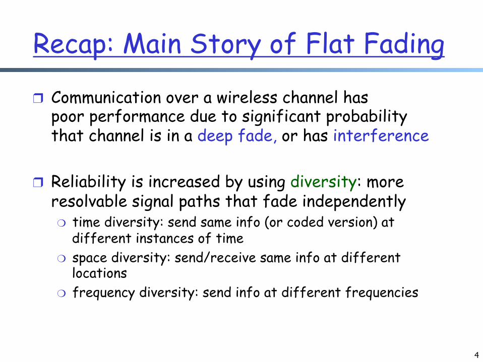
❒  Communication over a wireless channel has poor performance due to significant probability that channel is in a deep fade, or has interference

❒  Reliability is increased by using diversity: more resolvable signal paths that fade independently ❍  time diversity: send same info (or coded version) at

different instances of time ❍  space diversity: send/receive same info at different

locations ❍  frequency diversity: send info at different frequencies

5

Outline

❒ Admin. and recap ❒  Inter-Symbol Interference (ISI)

ISI

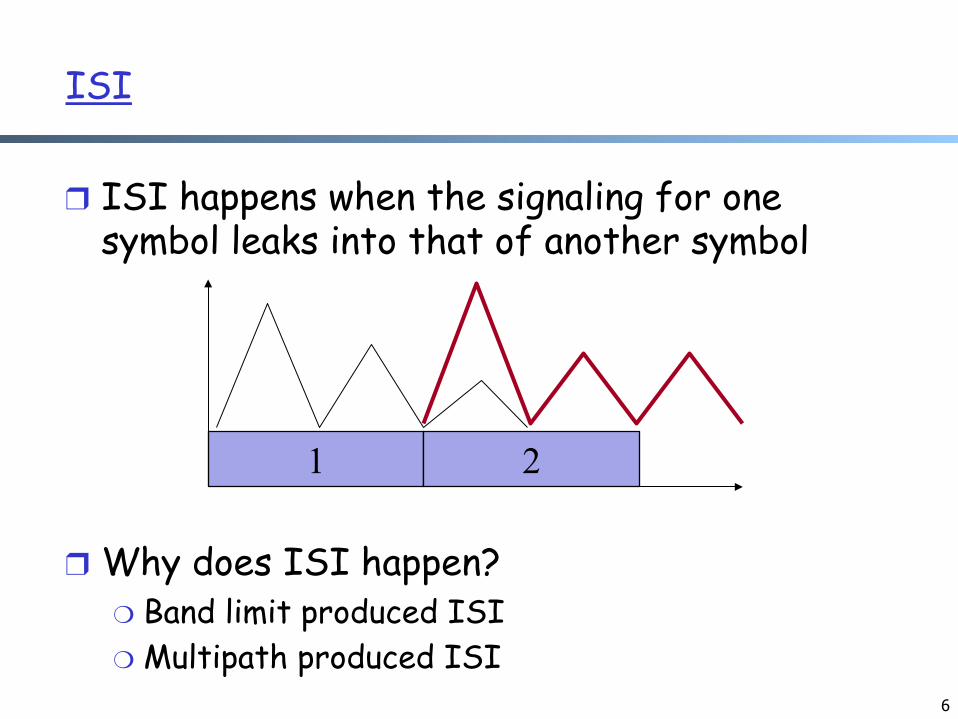
❒  ISI happens when the signaling for one symbol leaks into that of another symbol

❒ Why does ISI happen? ❍ Band limit produced ISI ❍ Multipath produced ISI

6

1 2

7

Outline

❒ Admin. and recap ❒  Inter-Symbol Interference (ISI)

❍ Bandlimit produced ISI

8

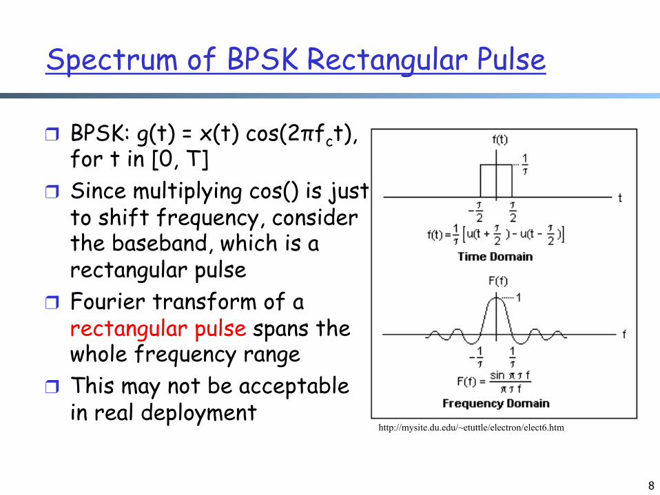
Spectrum of BPSK Rectangular Pulse

❒  BPSK: g(t) = x(t) cos(2πfct), for t in [0, T]

❒  Since multiplying cos() is just to shift frequency, consider the baseband, which is a rectangular pulse

❒  Fourier transform of a rectangular pulse spans the whole frequency range

❒  This may not be acceptable in real deployment

http://mysite.du.edu/~etuttle/electron/elect6.htm

9

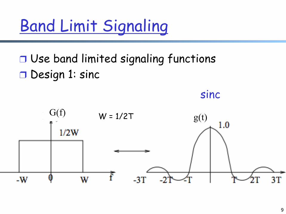
Band Limit Signaling

❒ Use band limited signaling functions ❒ Design 1: sinc

W = 1/2T

sinc

G(f) g(t)

10

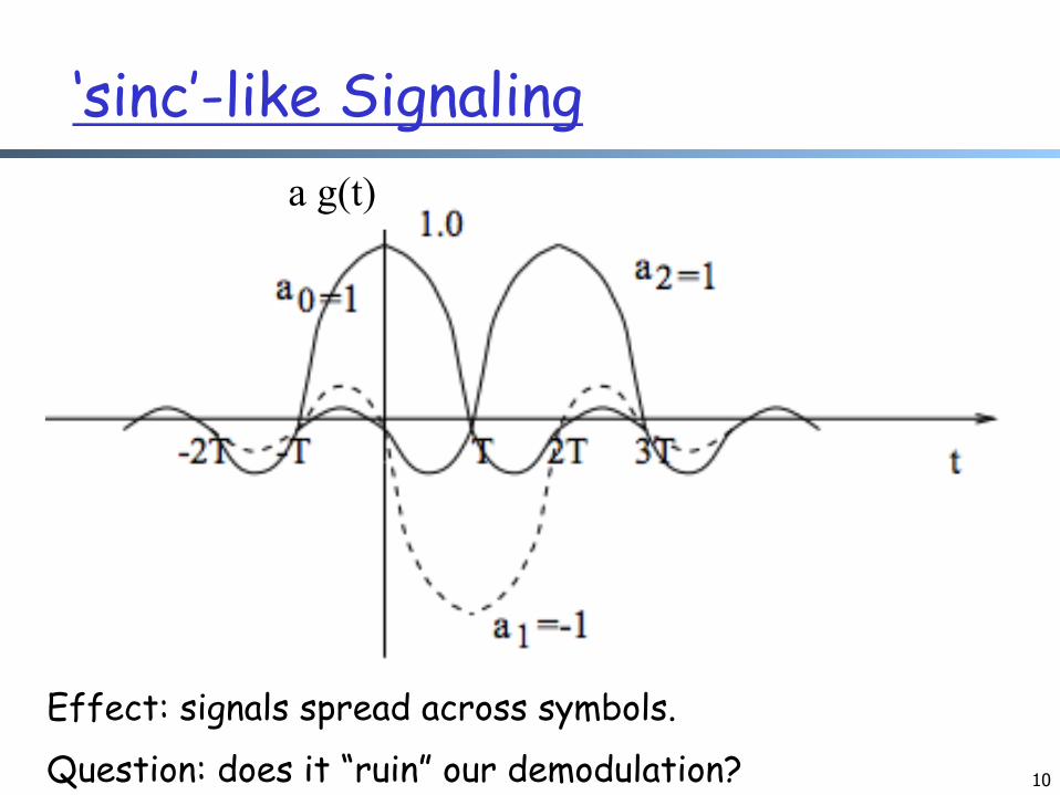
‘sinc’-like Signaling a g(t)

Effect: signals spread across symbols. Question: does it “ruin” our demodulation?

11

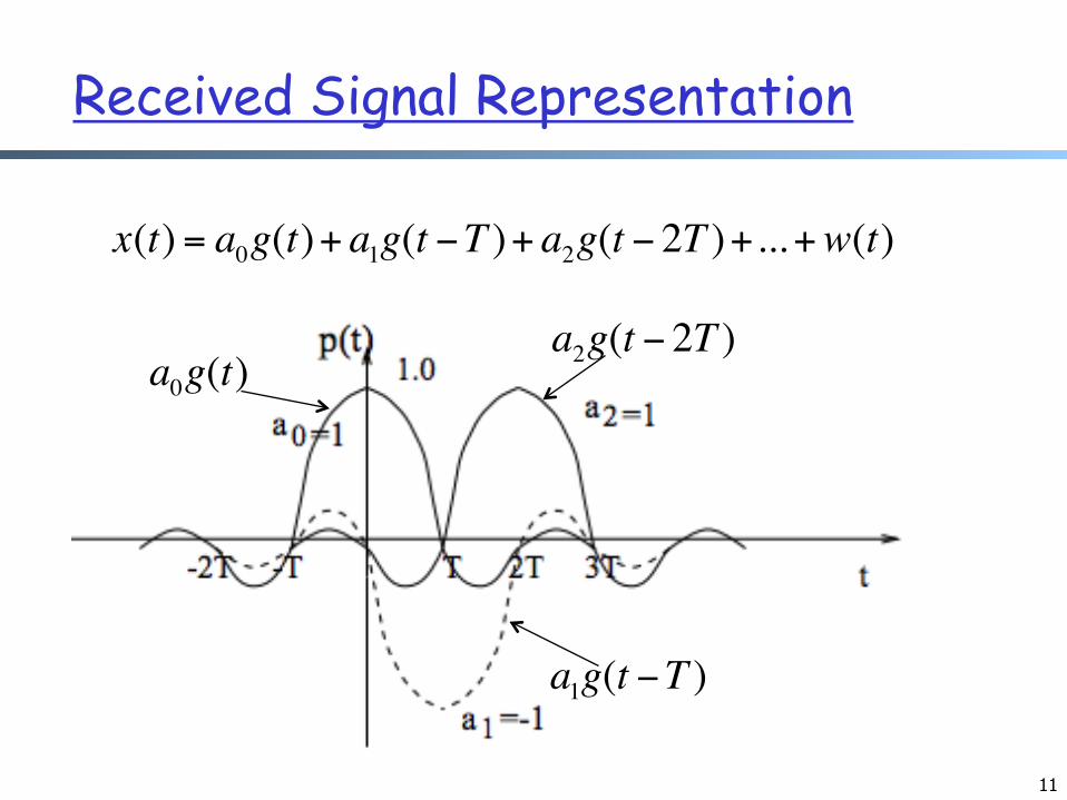
Received Signal Representation

x(t) = a0g(t)+ a1g(t −T )+ a2g(t − 2T )+...+w(t)

a0g(t)

a1g(t −T )

a2g(t − 2T )

12

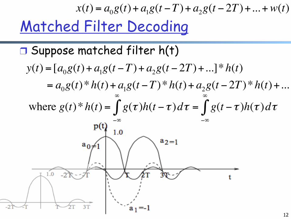
Matched Filter Decoding ❒ Suppose matched filter h(t)

x(t) = a0g(t)+ a1g(t −T )+ a2g(t − 2T )+...+w(t)

y(t) = [a0g(t)+ a1g(t −T )+ a2g(t − 2T )+...]*h(t)= a0g(t)*h(t)+ a1g(t −T )*h(t)+ a2g(t − 2T )*h(t)+...

where g(t)*h(t) = g(τ )h(t −τ )dτ−∞

∞

∫ = g(t −τ )h(τ )dτ−∞

∞

∫

13

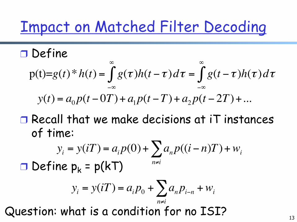
Impact on Matched Filter Decoding ❒ Define

❒  Recall that we make decisions at iT instances

of time: ❒ Define pk = p(kT)

y(t) = a0p(t − 0T )+ a1p(t −T )+ a2p(t − 2T )+...

p(t)=g(t)*h(t) = g(τ )h(t −τ )dτ−∞

∞

∫ = g(t −τ )h(τ )dτ−∞

∞

∫

yi = y(iT ) = ai p(0)+ anp((i− n)T )n≠i∑ +wi

yi = y(iT ) = ai p0 + anpi−nn≠i∑ +wi

Question: what is a condition for no ISI?

14

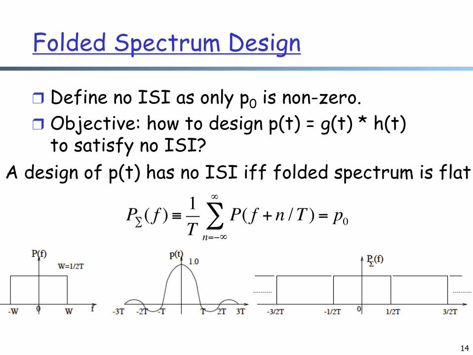
Folded Spectrum Design

❒ Define no ISI as only p0 is non-zero. ❒ Objective: how to design p(t) = g(t) * h(t)

to satisfy no ISI? A design of p(t) has no ISI iff folded spectrum is flat

P∑( f ) ≡1T

P( f + n /T ) = p0n=−∞

∞

∑

15

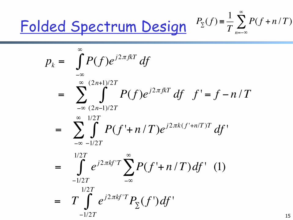
Folded Spectrum Design

pk = P( f )e j2π fkT df−∞

∞

∫

= P( f )e j2π fkT df(2n−1)/2T

(2n+1)/2T

∫−∞

∞

∑ f ' = f − n /T

= P( f '+ n /T )e j2πk ( f '+n/T )T df '−1/2T

1/2T

∫−∞

∞

∑

= e j2πkf 'T P( f '+ n /T )−∞

∞

∑ df '−1/2T

1/2T

∫ (1)

= T e j2πkf 'TP∑( f ')df−1/2T

1/2T

∫ '

P∑( f ) ≡1T

P( f + n /T )n=−∞

∞

∑

16

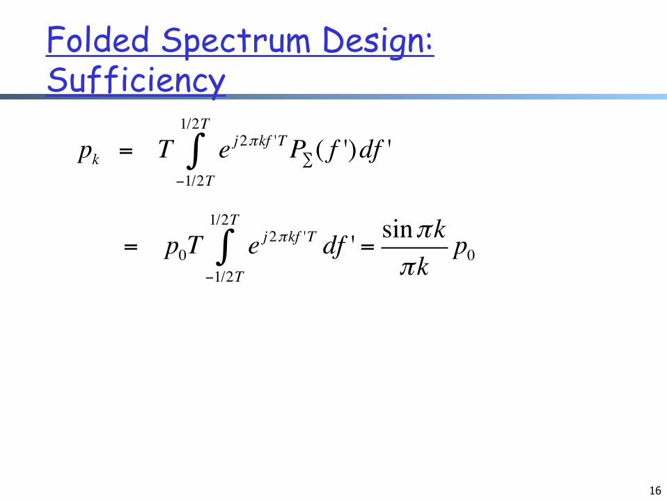
Folded Spectrum Design: Sufficiency

= p0T e j2πkf 'T df−1/2T

1/2T

∫ ' = sinπkπk

p0

pk = T e j2πkf 'TP∑( f ')df−1/2T

1/2T

∫ '

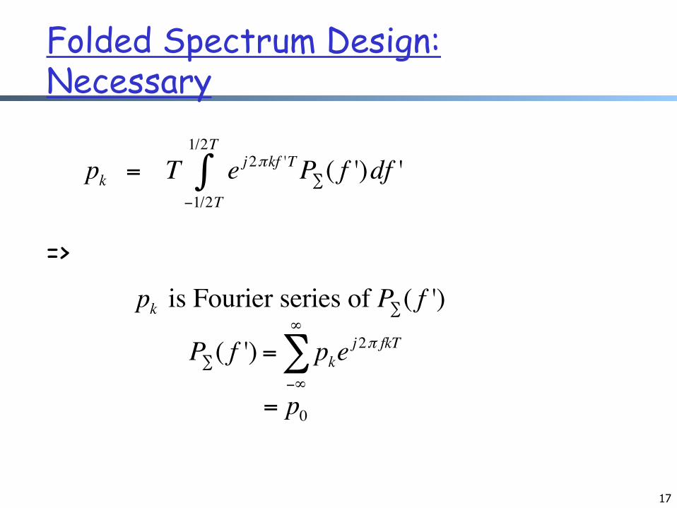
Folded Spectrum Design: Necessary

=>

17

pk is Fourier series of P∑( f ')

P∑( f ') = pk−∞

∞

∑ e j2π fkT

pk = T e j2πkf 'TP∑( f ')df−1/2T

1/2T

∫ '

= p0

18

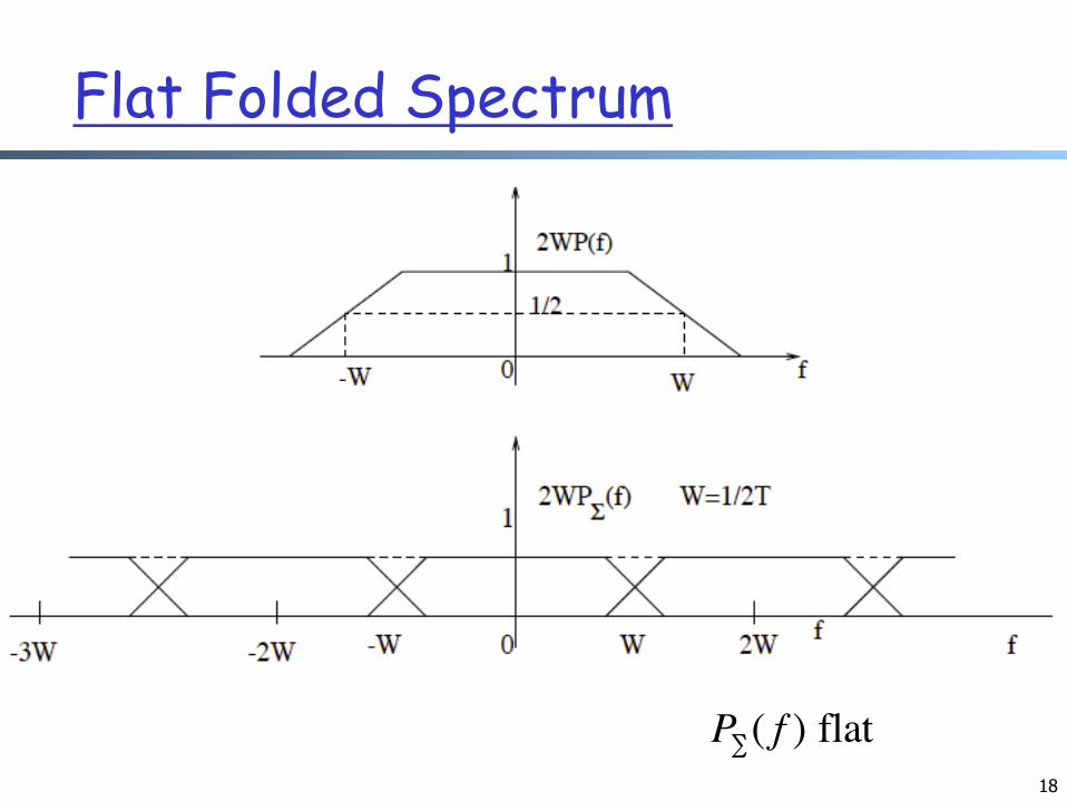
Flat Folded Spectrum

P∑( f ) flat

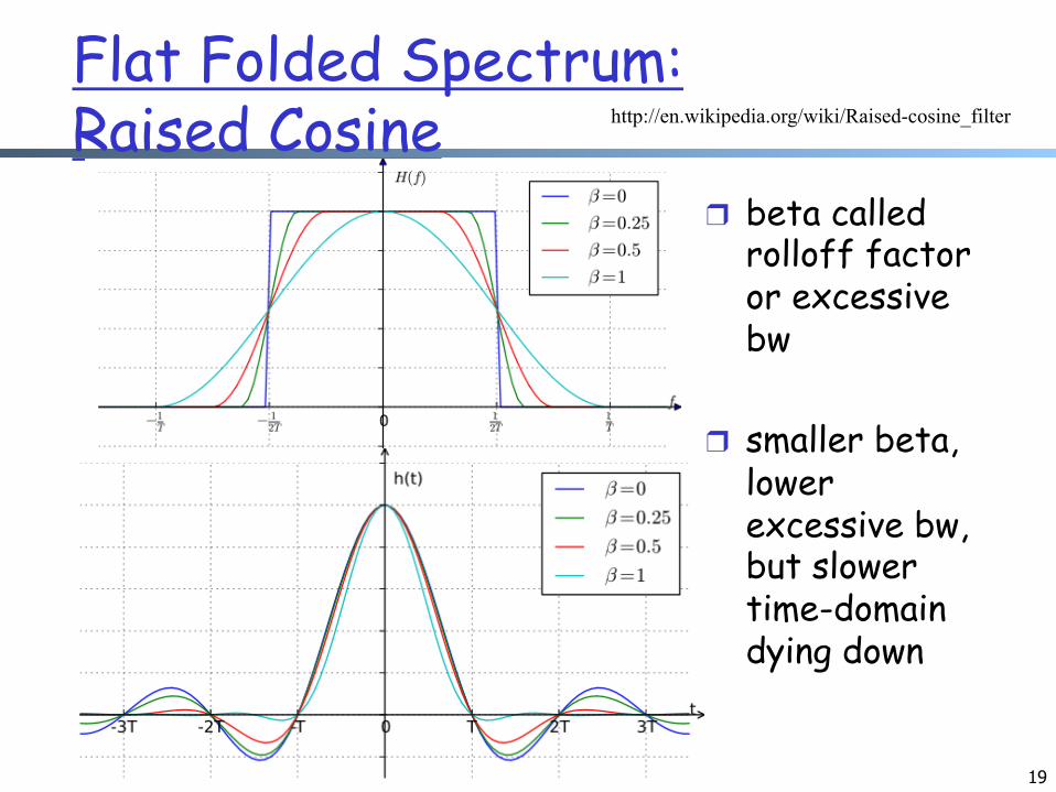
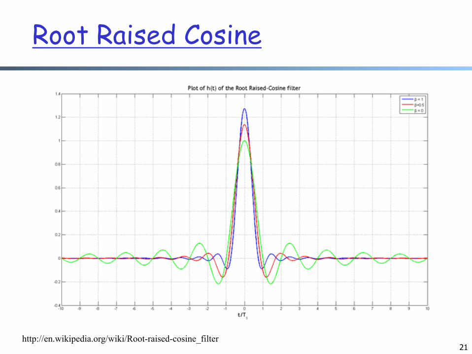
Flat Folded Spectrum: Raised Cosine

❒  beta called rolloff factor or excessive bw

❒  smaller beta, lower excessive bw, but slower time-domain dying down

19

http://en.wikipedia.org/wiki/Raised-cosine_filter

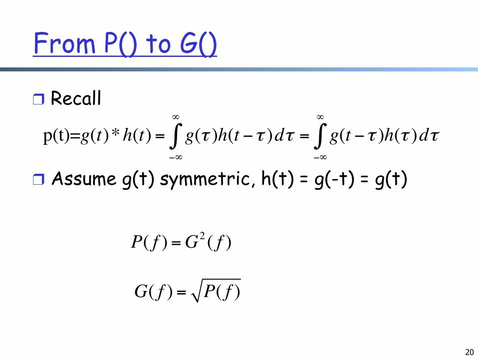
From P() to G()

❒  Recall

❒ Assume g(t) symmetric, h(t) = g(-t) = g(t)

20

p(t)=g(t)*h(t) = g(τ )h(t −τ )dτ−∞

∞

∫ = g(t −τ )h(τ )dτ−∞

∞

∫

P( f ) =G2 ( f )

G( f ) = P( f )

21

Root Raised Cosine

http://en.wikipedia.org/wiki/Root-raised-cosine_filter

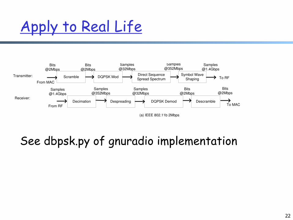
Apply to Real Life

See dbpsk.py of gnuradio implementation

22

InterleavingConvolutional

encoderQAM Mod IFFT GI Addition

Symbol WaveShaping

ScrambleTo RF

Direct SequenceSpread Spectrum

DQPSK ModSymbol Wave

ShapingScramble

(a) IEEE 802.11b 2Mbps

To RF

(b) IEEE 802.11a/g 24Mbps

Demod +Interleaving

FFTViterbi

decodingRemove GI

From RF

Descramble

DQPSK DemodDespreading Descramble

Transmitter:

Receiver:

Transmitter:

Receiver:

Samples@32Mbps

Samples@352Mbps

Samples@1.4Gbps

From RF

Samples@1.4Gbps

Decimation

Samples@352Mbps

Samples@32Mbps

Bits@2Mbps

Bits@48Mbps

Bits@48Mbps

Samples@512Mbps

Samples@1.28Gbps

Samples@640Mbps

Decimation

Samples@384Mbps

Bits@24Mbps

Bits@2Mbps

Samples@1.28Gbps

Samples@640Mbps

Samples@512Mbps

Samples@384Mbps

Bits@48Mbps

Bits@24Mbps

Bits@24Mbps

To MAC

From MAC

To MAC

Bits@2Mbps

Bits@2Mbps

Bits@24Mbps

From MAC

Figure 1: PHY operations of IEEE 802.11a/b/g transceiver.

functional blocks in their PHY components. Thesefunctional blocks are pipelined with one another. Dataare streamed through these blocks sequentially, but withdifferent data types and sizes. As illustrated in Figure 1,different blocks may consume or produce different typesof data in different rates arranged in small data blocks.For example, in 802.11b, the scrambler may consumeand produce one bit, while DQPSK modulation mapseach two-bit data block onto a complex symbol whichuses two 16-bit numbers to represent the in-phase andquadrature (I/Q) components.

Each PHY block performs a fixed amount of compu-tation on every transmitted or received bit. When thedata rate is high, e.g., 11Mbps for 802.11b and 54Mbpsfor 802.11a/g, PHY processing blocks consume a sig-nificant amount of computational power. Based on themodel in [19], we estimate that a direct implementationof 802.11b may require 10Gops while 802.11a/g needsat least 40Gops. These requirements are very demand-ing for software processing in GPPs.

PHY processing blocks directly operate on the dig-ital waveforms after modulation on the transmitter sideand before demodulation on the receiver side. Therefore,high-throughput interfaces are needed to connect theseprocessing blocks as well as to connect the PHY andradio front-end. The required throughput linearly scaleswith the bandwidth of the baseband signal. For example,the channel bandwidth is 20MHz in 802.11a. It requiresa data rate of at least 20M complex samples per secondto represent the waveform [14]. These complex samplesnormally require 16-bit quantization for both I and Qcomponents to provide sufficient fidelity, translating into32 bits per sample, or 640Mbps for the full 20MHz chan-nel. Over-sampling, a technique widely used for betterperformance [12], doubles the requirement to 1.28Gbps

to move data between the RF frond-end and PHY blocksfor one 802.11a channel.

2.2 Wireless MACThe wireless channel is a resource shared by alltransceivers operating on the same spectrum. As si-multaneously transmitting neighbors may interfere witheach other, various MAC protocols have been developedto coordinate their transmissions in wireless networks toavoid collisions.

Most modern MAC protocols, such as 802.11, requiretimely responses to critical events. For example, 802.11adopts a CSMA (Carrier-Sense Multiple Access) MACprotocol to coordinate transmissions [7]. Transmittersare required to sense the channel before starting theirtransmission, and channel access is only allowed whenno energy is sensed, i.e., the channel is free. The latencybetween sense and access should be as small as possible.Otherwise, the sensing result could be outdated and inac-curate. Another example is the link-layer retransmissionmechanisms in wireless protocols, which may require animmediate acknowledgement (ACK) to be returned in alimited time window.

Commercial standards like IEEE 802.11 mandate aresponse latency within tens of microseconds, which ischallenging to achieve in software on a general purposePC with a general purpose OS.

2.3 Software Radio RequirementsGiven the above discussion, we summarize the require-ments for implementing a software radio system on ageneral PC platform:High system throughput. The interfaces between theradio front-end and PHY as well as between somePHY processing blocks must possess sufficiently high

23

?

http://setemagali.com/2009/10/12/climbing-the-mountain-everyday/

24

Outline

❒ Admin. and recap ❒  Inter-Symbol Interference (ISI)

❍ Bandlimit ISI ❍ Multipath ISI

25

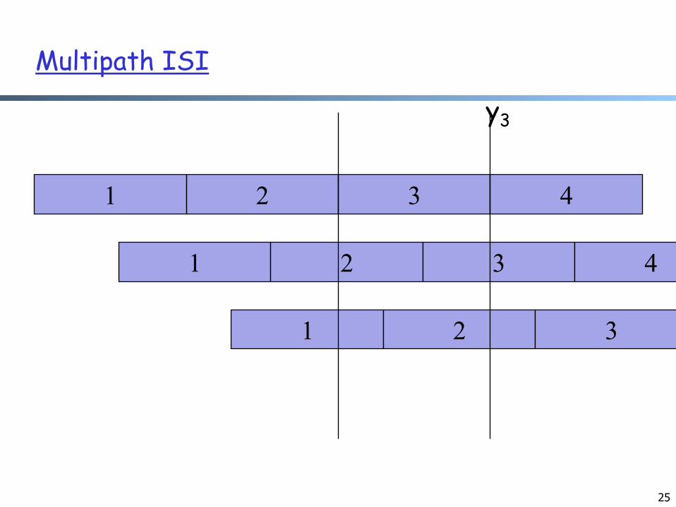
Multipath ISI

1 2 3 4

1 2 3 4

1 2 3 4

y3

26

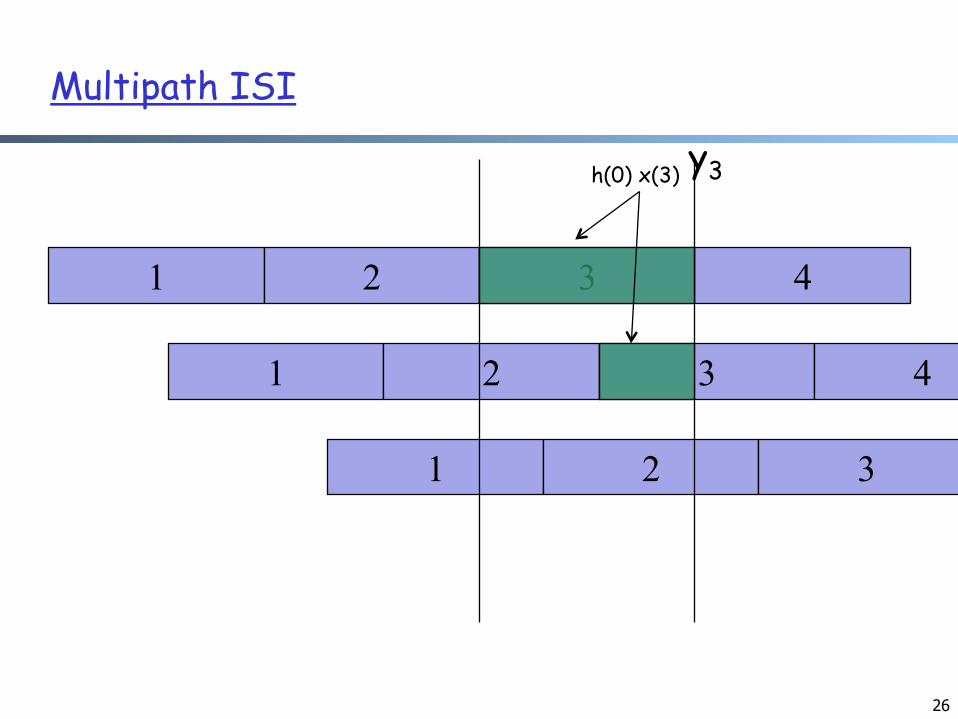
Multipath ISI

1 2 3 4

1 2 3 4

1 2 3 4

h(0) x(3) y3

27

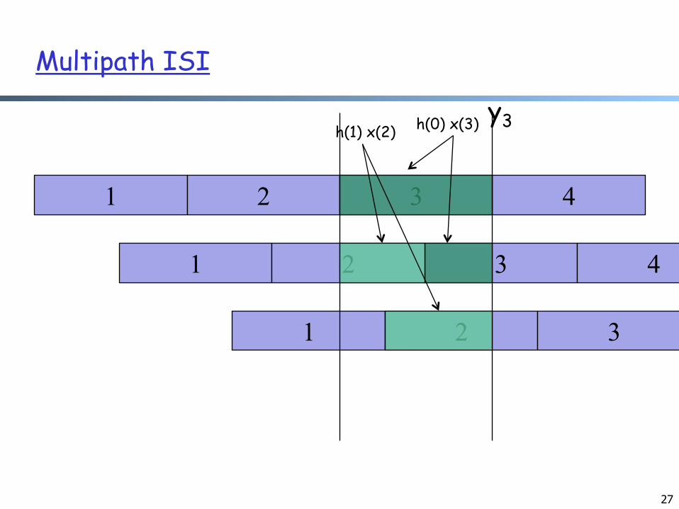
Multipath ISI

1 2 3 4

1 2 3 4

1 2 3 4

h(0) x(3) h(1) x(2) y3

28

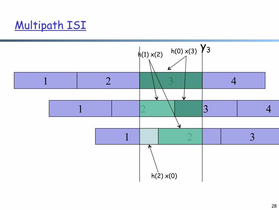
Multipath ISI

1 2 3 4

1 2 3 4

1 2 3 4

h(0) x(3) h(1) x(2) y3

h(2) x(0)

29

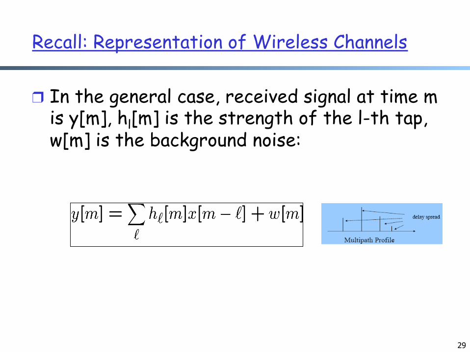
Recall: Representation of Wireless Channels

❒  In the general case, received signal at time m is y[m], hl[m] is the strength of the l-th tap, w[m] is the background noise:

30

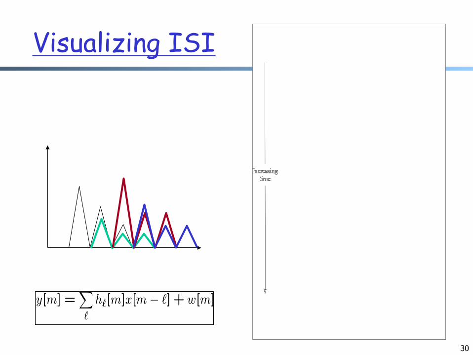
Visualizing ISI

31

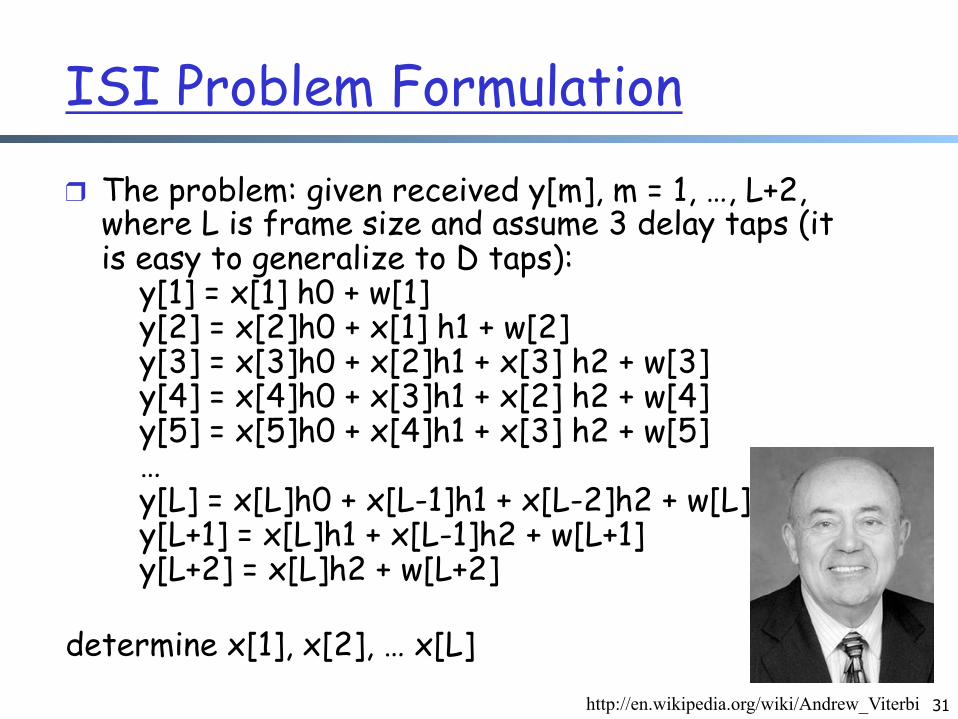
ISI Problem Formulation

❒  The problem: given received y[m], m = 1, …, L+2, where L is frame size and assume 3 delay taps (it is easy to generalize to D taps): y[1] = x[1] h0 + w[1] y[2] = x[2]h0 + x[1] h1 + w[2] y[3] = x[3]h0 + x[2]h1 + x[3] h2 + w[3] y[4] = x[4]h0 + x[3]h1 + x[2] h2 + w[4] y[5] = x[5]h0 + x[4]h1 + x[3] h2 + w[5] … y[L] = x[L]h0 + x[L-1]h1 + x[L-2]h2 + w[L] y[L+1] = x[L]h1 + x[L-1]h2 + w[L+1] y[L+2] = x[L]h2 + w[L+2]

determine x[1], x[2], … x[L] http://en.wikipedia.org/wiki/Andrew_Viterbi

32

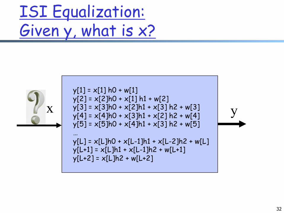
ISI Equalization: Given y, what is x?

y

y[1] = x[1] h0 + w[1] y[2] = x[2]h0 + x[1] h1 + w[2] y[3] = x[3]h0 + x[2]h1 + x[3] h2 + w[3] y[4] = x[4]h0 + x[3]h1 + x[2] h2 + w[4] y[5] = x[5]h0 + x[4]h1 + x[3] h2 + w[5] … y[L] = x[L]h0 + x[L-1]h1 + x[L-2]h2 + w[L] y[L+1] = x[L]h1 + x[L-1]h2 + w[L+1] y[L+2] = x[L]h2 + w[L+2]

x

33

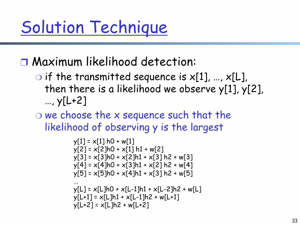
Solution Technique

❒ Maximum likelihood detection: ❍  if the transmitted sequence is x[1], …, x[L],

then there is a likelihood we observe y[1], y[2], …, y[L+2]

❍ we choose the x sequence such that the likelihood of observing y is the largest

y[1] = x[1] h0 + w[1] y[2] = x[2]h0 + x[1] h1 + w[2] y[3] = x[3]h0 + x[2]h1 + x[3] h2 + w[3] y[4] = x[4]h0 + x[3]h1 + x[2] h2 + w[4] y[5] = x[5]h0 + x[4]h1 + x[3] h2 + w[5] … y[L] = x[L]h0 + x[L-1]h1 + x[L-2]h2 + w[L] y[L+1] = x[L]h1 + x[L-1]h2 + w[L+1] y[L+2] = x[L]h2 + w[L+2]

34

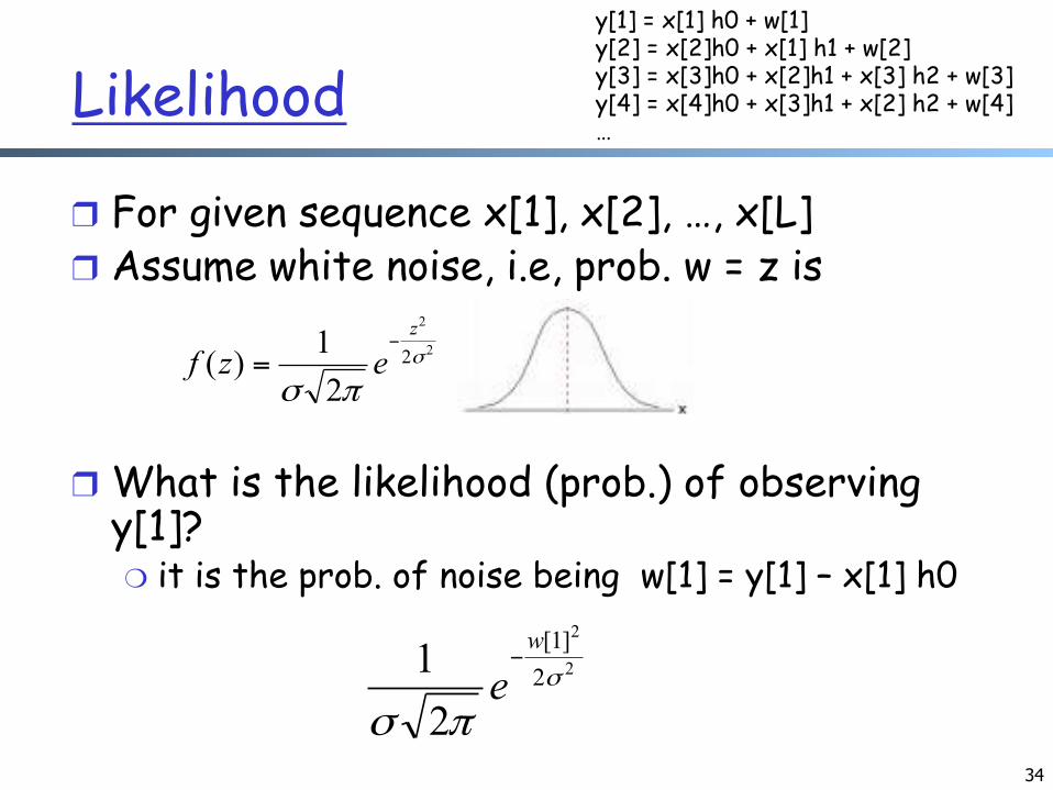
Likelihood

❒  For given sequence x[1], x[2], …, x[L] ❒ Assume white noise, i.e, prob. w = z is

❒ What is the likelihood (prob.) of observing y[1]? ❍  it is the prob. of noise being w[1] = y[1] – x[1] h0

2

2

2

21)( σ

πσ

z

ezf−

=

2

2

2]1[

21 σ

πσ

w

e−

y[1] = x[1] h0 + w[1] y[2] = x[2]h0 + x[1] h1 + w[2] y[3] = x[3]h0 + x[2]h1 + x[3] h2 + w[3] y[4] = x[4]h0 + x[3]h1 + x[2] h2 + w[4] …

35

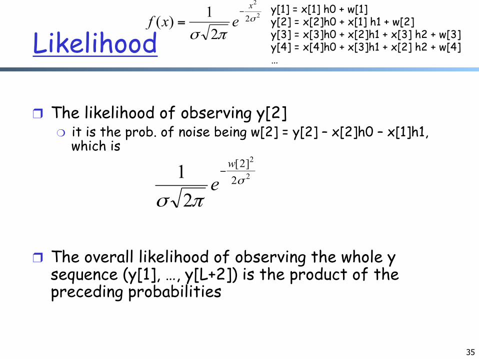
Likelihood

❒  The likelihood of observing y[2] ❍  it is the prob. of noise being w[2] = y[2] – x[2]h0 – x[1]h1,

which is

❒  The overall likelihood of observing the whole y sequence (y[1], …, y[L+2]) is the product of the preceding probabilities

2

2

2

21)( σ

πσ

x

exf−

=

2

2

2]2[

21 σ

πσ

w

e−

y[1] = x[1] h0 + w[1] y[2] = x[2]h0 + x[1] h1 + w[2] y[3] = x[3]h0 + x[2]h1 + x[3] h2 + w[3] y[4] = x[4]h0 + x[3]h1 + x[2] h2 + w[4] …

36

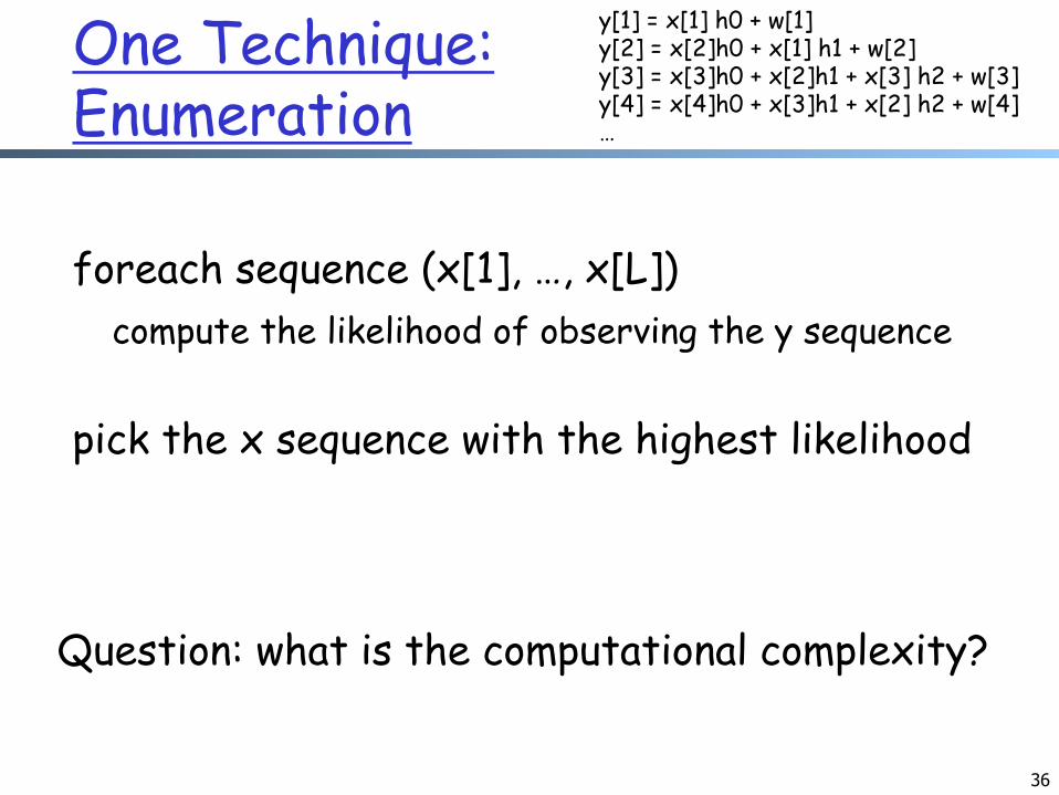
One Technique: Enumeration

foreach sequence (x[1], …, x[L]) compute the likelihood of observing the y sequence

pick the x sequence with the highest likelihood

Question: what is the computational complexity?

y[1] = x[1] h0 + w[1] y[2] = x[2]h0 + x[1] h1 + w[2] y[3] = x[3]h0 + x[2]h1 + x[3] h2 + w[3] y[4] = x[4]h0 + x[3]h1 + x[2] h2 + w[4] …

37

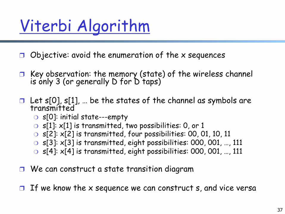
Viterbi Algorithm ❒  Objective: avoid the enumeration of the x sequences

❒  Key observation: the memory (state) of the wireless channel is only 3 (or generally D for D taps)

❒  Let s[0], s[1], … be the states of the channel as symbols are transmitted ❍  s[0]: initial state---empty ❍  s[1]: x[1] is transmitted, two possibilities: 0, or 1 ❍  s[2]: x[2] is transmitted, four possibilities: 00, 01, 10, 11 ❍  s[3]: x[3] is transmitted, eight possibilities: 000, 001, …, 111 ❍  s[4]: x[4] is transmitted, eight possibilities: 000, 001, …, 111

❒  We can construct a state transition diagram

❒  If we know the x sequence we can construct s, and vice versa

38

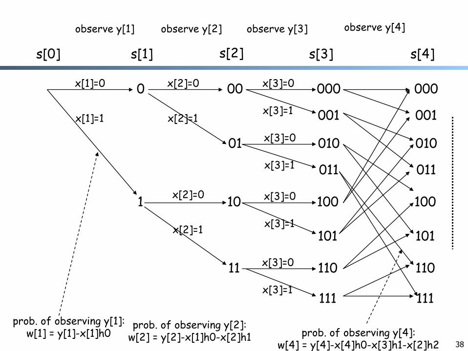
s[0] s[1] s[2] s[3] s[4]

0

1

00

01

10

11

000

010

100

110

001

011

101

111

000

010

100

110

001

011

101

111

x[1]=0

x[1]=1

x[2]=0

x[2]=1

x[2]=0

x[2]=1

x[3]=0

x[3]=1

x[3]=0

x[3]=1

x[3]=0

x[3]=1

x[3]=0

x[3]=1

observe y[1] observe y[2] observe y[3] observe y[4]

prob. of observing y[4]: w[4] = y[4]-x[4]h0-x[3]h1-x[2]h2

prob. of observing y[1]: w[1] = y[1]-x[1]h0

prob. of observing y[2]: w[2] = y[2]-x[1]h0-x[2]h1

39

Viterbi Algorithm

❒  Each path on the state-transition diagram corresponds to a x sequence ❍  each edge has a probability ❍  the product of the probabilities on the edges of a path

corresponds to the likelihood that we observe y if x is the sequence sent

❒  Then the problem becomes identifying the path with the largest product of probabilities

❒  If we take -log of the probability of each edge, the problem becomes identifying the shortest path problem!

Viterbi Algorithm: Summary

❒  Invented in 1967 ❒ Utilized in CDMA, GSM, 802.11, Dial-up

modem, and deep space communications

❒ Also commonly used in ❍  speech recognition, ❍  computational linguistics, and ❍  bioinformatics

40

Original paper: Andrew J. Viterbi. Error bounds for convolutional codes and an asymptotically optimum decoding algorithm, April 1967

http://ieeexplore.ieee.org/search/wrapper.jsp?arnumber=1054010

41

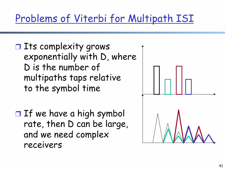
Problems of Viterbi for Multipath ISI

❒  Its complexity grows exponentially with D, where D is the number of multipaths taps relative to the symbol time

❒  If we have a high symbol rate, then D can be large, and we need complex receivers

42

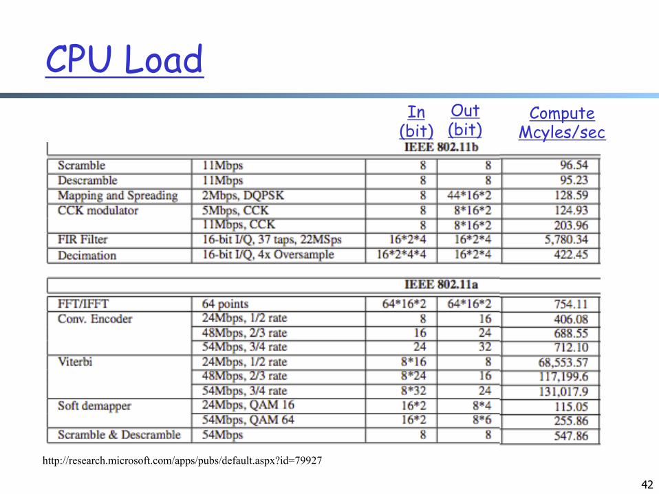
CPU Load In

(bit)

Out (bit)

Compute Mcyles/sec

http://research.microsoft.com/apps/pubs/default.aspx?id=79927