HANDBOOK OF COMPUTER SCIENCE AND ENGINEERING Chapter 6 Pattern matching and text
57
HANDBOOK OF COMPUTER SCIENCE AND ENGINEERING Chapter 6 Pattern matching and text compression algorithms
Transcript of HANDBOOK OF COMPUTER SCIENCE AND ENGINEERING Chapter 6 Pattern matching and text

HANDBOOK OF COMPUTER SCIENCE ANDENGINEERING
Chapter 6Pattern matching and text compression algorithms

Contents
6 Pattern matching and text compression algorithms 56.1 Processing texts efficiently . . . . . . . . . . . . . . . . . . . . . . . . . . . . . . . . 56.2 String-matching algorithms . . . . . . . . . . . . . . . . . . . . . . . . . . . . . . . . 6
6.2.1 Karp-Rabin algorithm . . . . . . . . . . . . . . . . . . . . . . . . . . . . . . 66.2.2 Knuth-Morris-Pratt algorithm . . . . . . . . . . . . . . . . . . . . . . . . . . 86.2.3 Boyer-Moore algorithm . . . . . . . . . . . . . . . . . . . . . . . . . . . . . 96.2.4 Quick Search algorithm . . . . . . . . . . . . . . . . . . . . . . . . . . . . . 136.2.5 Experimental results . . . . . . . . . . . . . . . . . . . . . . . . . . . . . . . 146.2.6 Aho-Corasick algorithm . . . . . . . . . . . . . . . . . . . . . . . . . . . . . 14
6.3 Two-dimensional pattern matching algorithms . . . . . . . . . . . . . . . . . . . . . . 186.3.1 Zhu-Takaoka algorithm . . . . . . . . . . . . . . . . . . . . . . . . . . . . . . 196.3.2 Bird/Baker algorithm . . . . . . . . . . . . . . . . . . . . . . . . . . . . . . . 22
6.4 Suffix trees . . . . . . . . . . . . . . . . . . . . . . . . . . . . . . . . . . . . . . . . 256.4.1 McCreight algorithm . . . . . . . . . . . . . . . . . . . . . . . . . . . . . . . 27
6.5 Longest common subsequence of two strings . . . . . . . . . . . . . . . . . . . . . . 286.5.1 Dynamic programming . . . . . . . . . . . . . . . . . . . . . . . . . . . . . . 316.5.2 Reducing the space: Hirschberg algorithm . . . . . . . . . . . . . . . . . . . . 33
6.6 Approximate string matching . . . . . . . . . . . . . . . . . . . . . . . . . . . . . . . 346.6.1 Shift-Or algorithm . . . . . . . . . . . . . . . . . . . . . . . . . . . . . . . . 366.6.2 String matching with
�mismatches . . . . . . . . . . . . . . . . . . . . . . . 37
6.6.3 String matching with�
differences . . . . . . . . . . . . . . . . . . . . . . . . 386.6.4 Wu-Manber algorithm . . . . . . . . . . . . . . . . . . . . . . . . . . . . . . 40
6.7 Text compression . . . . . . . . . . . . . . . . . . . . . . . . . . . . . . . . . . . . . 416.7.1 Huffman coding . . . . . . . . . . . . . . . . . . . . . . . . . . . . . . . . . 416.7.2 LZW Compression . . . . . . . . . . . . . . . . . . . . . . . . . . . . . . . . 486.7.3 Experimental results . . . . . . . . . . . . . . . . . . . . . . . . . . . . . . . 52
6.8 Research Issues and Summary . . . . . . . . . . . . . . . . . . . . . . . . . . . . . . 526.9 Defining Terms . . . . . . . . . . . . . . . . . . . . . . . . . . . . . . . . . . . . . . 536.10 References . . . . . . . . . . . . . . . . . . . . . . . . . . . . . . . . . . . . . . . . . 546.11 Further Information . . . . . . . . . . . . . . . . . . . . . . . . . . . . . . . . . . . . 55
1

2 CONTENTS

List of Figures
6.1 The brute force string-matching algorithm. . . . . . . . . . . . . . . . . . . . . . . . . 66.2 The Karp-Rabin string-matching algorithm. . . . . . . . . . . . . . . . . . . . . . . . 76.3 Shift in the Knuth-Morris-Pratt algorithm ( � suffix of � ). . . . . . . . . . . . . . . . . 86.4 The Knuth-Morris-Pratt string-matching algorithm. . . . . . . . . . . . . . . . . . . . 96.5 Preprocessing phase of the Knuth-Morris-Pratt algorithm: computing next. . . . . . . 96.6 good-suffix shift, � reappears preceded by a character different from
�. . . . . . . . . . 10
6.7 good-suffix shift, only a suffix of � reappears as a prefix of � . . . . . . . . . . . . . . . 106.8 bad-character shift, � appears in � . . . . . . . . . . . . . . . . . . . . . . . . . . . . . 106.9 bad-character shift, � does not appear in � . . . . . . . . . . . . . . . . . . . . . . . . . 116.10 The Boyer-Moore string-matching algorithm. . . . . . . . . . . . . . . . . . . . . . . 126.11 Computation of the bad-character shift. . . . . . . . . . . . . . . . . . . . . . . . . . 126.12 Computation of the good-suffix shift. . . . . . . . . . . . . . . . . . . . . . . . . . . . 136.13 The Quick Search string-matching algorithm. . . . . . . . . . . . . . . . . . . . . . . 146.14 Running times for a DNA sequence. . . . . . . . . . . . . . . . . . . . . . . . . . . . 156.15 Running times for an english text. . . . . . . . . . . . . . . . . . . . . . . . . . . . . 166.16 Preprocessing phase of the Aho-Corasick algorithm. . . . . . . . . . . . . . . . . . . . 166.17 Construction of the trie. . . . . . . . . . . . . . . . . . . . . . . . . . . . . . . . . . . 176.18 Completion of the output function and construction of failure links. . . . . . . . . . . . 176.19 The complete Aho-Corasick algorithm. . . . . . . . . . . . . . . . . . . . . . . . . . 196.20 The brute force two-dimensional pattern matching algorithm. . . . . . . . . . . . . . . 196.21 Search for ��� in ��� using KMP algorithm. . . . . . . . . . . . . . . . . . . . . . . . . 216.22 Naive check of an occurrence of � in � at position � ������������������� . . . . . . . . . . . . 216.23 The Zhu-Takaoka two-dimensional pattern matching algorithm. . . . . . . . . . . . . 226.24 Computes the function ������ for rows of ! . . . . . . . . . . . . . . . . . . . . . . . . 236.25 The Bird/Baker two-dimensional pattern matching algorithm. . . . . . . . . . . . . . . 246.26 Construction of a suffix tree for � . . . . . . . . . . . . . . . . . . . . . . . . . . . . . 256.27 Insertion of a new suffix in the tree. . . . . . . . . . . . . . . . . . . . . . . . . . . . 266.28 Suffix tree construction. . . . . . . . . . . . . . . . . . . . . . . . . . . . . . . . . . . 296.29 Initialization procedure. . . . . . . . . . . . . . . . . . . . . . . . . . . . . . . . . . . 296.30 The crucial rescan operation. . . . . . . . . . . . . . . . . . . . . . . . . . . . . . . . 306.31 Breaking an edge. . . . . . . . . . . . . . . . . . . . . . . . . . . . . . . . . . . . . . 306.32 The scan operation. . . . . . . . . . . . . . . . . . . . . . . . . . . . . . . . . . . . . 316.33 Dynamic programming algorithm to compute �"�"�$#%����&�'�)(+*-, �.�&�0/ . . . . . . . . . . . 326.34 Production of an �"�$#%����&�'� . . . . . . . . . . . . . . . . . . . . . . . . . . . . . . . . . 326.35 12"354768��.�&���&� -space algorithm to compute �"���$#�����&�9� . . . . . . . . . . . . . . . . . . 336.36 Computation of *;: . . . . . . . . . . . . . . . . . . . . . . . . . . . . . . . . . . . . . 346.37 12"354768��.�&���&� -space computation of �"�$#%����&�'� . . . . . . . . . . . . . . . . . . . . . . 356.38 Meaning of vector <>=? . . . . . . . . . . . . . . . . . . . . . . . . . . . . . . . . . . . 36
3

4 LIST OF FIGURES
6.39 If < =? � � , ����� /0(� then < �? , � /0(� . . . . . . . . . . . . . . . . . . . . . . . . . . . . . 386.40 < �? , � / (+< �? � � , ����� / if � , � /0( � , � / . . . . . . . . . . . . . . . . . . . . . . . . . . . . . 386.41 If < =? � � , ����� /0(� then < �? , � /0(� . . . . . . . . . . . . . . . . . . . . . . . . . . . . . 396.42 < �? , � / (+< �? � � , ����� / if � , � /0( � , � / . . . . . . . . . . . . . . . . . . . . . . . . . . . . . 396.43 If < =? , ����� / (� then < �? , � /8(� . . . . . . . . . . . . . . . . . . . . . . . . . . . . . . 406.44 < �? , � / (+< �? � � , ����� / if � , � /0( � , � / . . . . . . . . . . . . . . . . . . . . . . . . . . . . . 406.45 Wu-Manber approximate string-matching algorithm. . . . . . . . . . . . . . . . . . . 426.46 Counts the character frequencies. . . . . . . . . . . . . . . . . . . . . . . . . . . . . . 436.47 Builds the coding tree. . . . . . . . . . . . . . . . . . . . . . . . . . . . . . . . . . . 446.48 Builds the character codes from coding tree. . . . . . . . . . . . . . . . . . . . . . . . 456.49 Memorizes the coding tree in the compressed file. . . . . . . . . . . . . . . . . . . . . 456.50 Encodes the characters in the compressed file. . . . . . . . . . . . . . . . . . . . . . . 456.51 Complete function for Huffman coding. . . . . . . . . . . . . . . . . . . . . . . . . . 456.52 Rebuilds the tree read from the compressed file. . . . . . . . . . . . . . . . . . . . . . 476.53 Reads the compressed text and produces the uncompressed text. . . . . . . . . . . . . 476.54 Complete function for decoding. . . . . . . . . . . . . . . . . . . . . . . . . . . . . . 486.55 LZW compression algorithm. . . . . . . . . . . . . . . . . . . . . . . . . . . . . . . . 506.56 LZW decompression algorithm. . . . . . . . . . . . . . . . . . . . . . . . . . . . . . 516.57 Sizes of texts compressed with three algorithms. . . . . . . . . . . . . . . . . . . . . . 52

Chapter 6
Pattern matching and text compressionalgorithms
MAXIME CROCHEMORE, Gaspard Monge Institute, University of Marne-la-Vallee, FranceTHIERRY LECROQ, Laboratoire d’Informatique de Rouen, University of Rouen, France
6.1 Processing texts efficiently
The present chapter describes a few standard algorithms used for processing texts. They apply, forexample, to the manipulation of texts (word editors), to the storage of textual data (text compression),and to data retrieval systems. The algorithms of the chapter are interesting in different respects. First,they are basic components used in the implementations of practical software. Second, they introduceprogramming methods that serve as paradigms in other fields of computer science (system or softwaredesign). Third, they play an important role in theoretical computer science by providing challengingproblems.
Although data are stored in various ways, text remains the main form of exchanging information.This is particularly evident in literature or linguistics where data are composed of huge corpora anddictionaries. This applies as well to computer science where a large amount of data are stored inlinear files. And this is also the case in molecular biology where biological molecules can often beapproximated as sequences of nucleotides or amino-acids. Moreover, the quantity of available data inthese fields tends to double every eighteen months. This is the reason why algorithms should be efficienteven if the speed of computers increases regularly.
Pattern matching is the problem of locating a specific pattern inside raw data. The pattern is usuallya collection of strings described in some formal language. Two kinds of textual patterns are presented:single strings and approximated strings. We also present two algorithms for matching patterns in imagesthat are extensions of string-matching algorithms.
In several applications, texts need to be structured before being searched. Even if no further in-formation is known about their syntactic structure, it is possible and indeed extremely efficient to builta data structure that supports searches. ¿From among several existing data structures equivalent toindexes, we present the suffix tree, along with its construction.
The comparison of strings is implicit in the approximate pattern searching problem. Since it issometimes required to compare just two strings (files, or molecular sequences) we introduce the basicmethod based on longest common subsequences.
Finally, the chapter contains two classical text compression algorithms. Variants of these algorihmsare implemented in practical compression software, in which they are often combined together or with
5

6 CHAPTER 6. PATTERN MATCHING AND TEXT COMPRESSION ALGORITHMS
void BF(char *y, char *x, int n, int m) {int i, j;
/* Searching */for (i=0; i <= n-m; i++) {
j=0;while (j < m && y[i+j] == x[j]) j++;if (j >= m) OUTPUT(i);
}}
Figure 6.1: The brute force string-matching algorithm.
other elementary methods.The efficiency of algorithms is evaluated by their running times, and sometimes also by the amount
of memory space they require at run time.
6.2 String-matching algorithms
String matching consists of finding one, or more generally, all the occurrences of a pattern in a text.The pattern and the text are both strings built over a finite alphabet (a finite set of symbols). Eachalgorithm of this section outputs all occurrences of the pattern in the text. The pattern is denoted by� ( � , ������� � � � / ; its length is equal to � . The text is denoted by � ( � , ������� � � � / ; its length isequal to � . The alphabet is denoted by
�and its size is equal to � .
String-matching algorithms of the present section work as follows: they first align the left ends ofthe pattern and the text, then compare the aligned symbols of the text and the pattern — this specificwork is called an attempt or a scan — and after a whole match of the pattern or after a mismatch theyshift the pattern to the right. They repeat the same procedure again until the right end of the patterngoes beyond the right end of the text. This is called the scan and shift mechanism. We associate eachattempt with the position � in the text when the pattern is aligned with �0, ������� ��� � � � / .
The brute force algorithm consists of checking, at all positions in the text between 0 and � � � ,whether an occurrence of the pattern starts there or not. Then, after each attempt, it shifts the patternexactly one position to the right. This is the simplest algorithm, which is described in Figure 6.1.
The time complexity of the brute force algorithm is 15������ in the worst case but its behavior inpractice is often linear on specific data.
6.2.1 Karp-Rabin algorithm
Hashing provides a simple method for avoiding a quadratic number of symbol comparisons in mostpractical situations. Instead of checking at each position of the text whether the pattern occurs, it seemsto be more efficient to check only if the portion of the text aligned with the pattern “looks like” thepattern. In order to check the resemblance between these portions a hashing function is used. To behelpful for the string-matching problem the hashing function should have the following properties:
� efficiently computable,� highly discriminating for strings,

6.2. STRING-MATCHING ALGORITHMS 7
#define REHASH(a, b, h) (((h-a*d)<<1)+b)
void KR(char *y, char *x, int n, int m) {int hy, hx, d, i;
/* Preprocessing *//* computes d = 2ˆ(m-1) with the left-shift operator */d=1;for (i=1; i < m; i++) d<<=1;
hy=hx=0;for (i=0; i < m; i++) {
hx=((hx<<1)+x[i]);hy=((hy<<1)+y[i]);
}
/* Searching */for (i=m; i <= n; i++) {
if (hy == hx && strncmp(y+i-m, x, m) == 0) OUTPUT(i-m);hy=REHASH(y[i-m], y[i], hy);
}}
Figure 6.2: The Karp-Rabin string-matching algorithm.
��� ��# � �� , � � � ����� � � � /�� must be easily computable from � � # � ��0, ������� ��� � ��� /�� :� ��# � �� , � � � ����� � � � /�� ( � � � # � �� , � / �&�0, � � � / � � ��# � �� , � ����� ��� � ��� /��&� .
For a word � of length�
, its symbols can be considered as digits, and we define � ��# � �� � by:
� � # � �� , ������� � ��� /�� ( �� , ��/����� � � � � , � /����
� ��� ���� � � , � ��� /�� mod ���
where � is a large number. Then, � � � # � has a simple expression
� � � # � "��� � � � � ( & � � ���� ����� � � � mod �%�
where (�� � � � .During the search for the pattern � , it is enough to compare � ��# � �� � with � � # � ��0, � ����� � � � � � /��
for ��� ��� � � � . If an equality is found, it is still necessary to check the equality � (+�0, � ����� � � � � � /symbol by symbol.
In the algorithm of Figure 6.2 all the multiplications by � are implemented by shifts. Furthermore,the computation of the modulus function is avoided by using the implicit modular arithmetic given bythe hardware that forgets carries in integer operations. So, � is chosen as the maximum value of aninteger.
The worst-case time complexity of the Karp-Rabin algorithm is quadratic in the worst case (as it isfor the brute force algorithm) but its expected running time is 12�� � ��� .Example 6.1:Let � (������ .Then � � # � ��0� ( � ������� � � � � ����� � � ����( ��!"� (symbols are assimilated with their ASCII codes).

8 CHAPTER 6. PATTERN MATCHING AND TEXT COMPRESSION ALGORITHMS
�
�
�
�
��
�(
�(
� ��� �
�
�
�
Figure 6.3: Shift in the Knuth-Morris-Pratt algorithm ( � suffix of � ).
�2( s t r i n g m a t c h i n g� ��# � ( 806 797 776 743 678 585 443 746 719 766 709 736 743
6.2.2 Knuth-Morris-Pratt algorithm
This section presents the first discovered linear-time string-matching algorithm. Its design follows atight analysis of the brute force algorithm, and especially on the way this latter algorithm wastes theinformation gathered during the scan of the text.
Let us look more closely at the brute force algorithm. It is possible to improve the length of shiftsand simultaneously remember some portions of the text that match the pattern. This saves comparisonsbetween characters of the text and of the pattern, and consequently increases the speed of the search.
Consider an attempt at position � , that is, when the pattern � , ������� � � � / is aligned with the window� , � ����� � �.� � � / on the text. Assume that the first mismatch occurs between symbols � , � � � / and � , � /for��� ��� � . Then, � , � ����� � � � � � /;( � , ������� � � � /;( � and � ( �0, � � � / �( � , � /;( �
. Whenshifting, it is reasonable to expect that a prefix � of the pattern matches some suffix of the portion � ofthe text. Moreover, if we want to avoid another immediate mismatch, the letter following the prefix �in the pattern must be different from
�. The longest such prefix � is called the border of � (it occurs at
both ends of � ). This introduces the notation: let ������ $, � / be the length of the longest (proper) borderof � , ������� � � � / followed by a character � different from � , � / . Then, after a shift, the comparisonscan resume between characters �0, � � � / and � , ������ $, � / / without missing any occurrence of � in � , andavoiding a backtrack on the text (see Figure 6.3).

6.2. STRING-MATCHING ALGORITHMS 9
void KMP(char *y, char *x, int n, int m) {/* XSIZE is the maximum size of a pattern */int i, j, next[XSIZE];
/* Preprocessing */PRE_KMP(x, m, next);
/* Searching */i=j=0;while (i < n) {
while (j > -1 && x[j] != y[i]) j=next[j];i++; j++;if (j >= m) { OUTPUT(i-j); j=next[m]; }
}}
Figure 6.4: The Knuth-Morris-Pratt string-matching algorithm.
void PRE_KMP(char *x, int m, int next[]) {int i, j;
i=0; j=next[0]=-1;while (i < m) {
while (j > -1 && x[i] != x[j]) j=next[j];i++; j++;if (i < m && x[i] == x[j]) next[i]=next[j];else next[i]=j;
}}
Figure 6.5: Preprocessing phase of the Knuth-Morris-Pratt algorithm: computing next.
Example 6.2:�2( . . . a b a b a a . . . . . .� ( a b a b a b a� ( a b a b a b a
Compared symbols are underlined. Note that the empty string is the suitable border of ababa. Otherborders of ababa are aba and a.
The Knuth-Morris-Pratt algorithm is displayed in Figure 6.4. The table ���$�� it uses is computedin 15�� � time before the search phase, applying the same searching algorithm to the pattern itself, asif � ( � (see Figure 6.5). The worst-case running time of the algorithm is 12�� � ��� and it requires12�� � extra-space. These quantities are independent of the size of the underlying alphabet.
6.2.3 Boyer-Moore algorithm
The Boyer-Moore algorithm is considered the most efficient string-matching algorithm in usual appli-cations. A simplified version of it, or the entire algorithm, is often implemented in text editors for the

10 CHAPTER 6. PATTERN MATCHING AND TEXT COMPRESSION ALGORITHMS
�
�
�
�
��
�(
�(
�
�
�shift
Figure 6.6: good-suffix shift, � reappears preceded by a character different from�.
�
�
��( ��
�
�
�
shift
Figure 6.7: good-suffix shift, only a suffix of � reappears as a prefix of � .
“search” and “substitute” commands.The algorithm scans the characters of the pattern from right to left beginning with the rightmost
symbol. In case of a mismatch (or a complete match of the whole pattern) it uses two precomputedfunctions to shift the pattern to the right. These two shift functions are called the bad-character shiftand the good-suffix shift. They are based on the following observations.
Assume that a mismatch occurs between the character � , � /0( �of the pattern and the character � , ���� / (+� of the text during an attempt at position � . Then, � , � � � � � ����� � � � � � /0(+� , � � � ����� � � � / ( �
and �0, � � � / �( � , � / . The good-suffix shift consists of aligning the segment � , � � � � � ����� � � � � � /0(� , � � � ����� � � � / with its rightmost occurrence in � that is preceded by a character different from � , � /(see Figure 6.6). If there exists no such segment, the shift consists of aligning the longest suffix � of� , � � � � � ����� � � � � � / with a matching prefix of � (see Figure 6.7).
�
�
�
�
���(
contains no �
�
�shift
Figure 6.8: bad-character shift, � appears in � .

6.2. STRING-MATCHING ALGORITHMS 11
�
�
����(
contains no �
�
�shift
Figure 6.9: bad-character shift, � does not appear in � .
Example 6.3:�2( . . . a b b a a b b a b b a . . .� ( a b b a a b b a b b a� ( a b b a a b b a b b a
The shift is driven by the suffix abba of � found in the text. After the shift, the segment abba in themiddle of � matches a segment of � as in Figure 6.6. The same mismatch does not recur.
Example 6.4:�2( . . . a b b a a b b a b b a b b a . .� ( b b a b b a b b a� ( b b a b b a b b a
The segment abba found in � partially matches a prefix of � after the shift, like in Figure 6.7.
The bad-character shift consists of aligning the text character � , � � � / with its rightmost occurrencein � , ������� � � � / (see Figure 6.8). If � , � � � / does not appear in the pattern � , no occurrence of � in �can overlap the symbol � , � � � / , then, the left end of the pattern is aligned with the character at position� � � � � (see Figure 6.9).
Example 6.5:�2( . . . . . . a b c d . . . .� ( c d a h g f e b c d� ( c d a h g f e b c d
The shift aligns the symbol a in � with the mismatch symbol a in the text � (Figure 6.8).
Example 6.6:�2( . . . . . a b c d . . . . . .� ( c d h g f e b c d� ( c d h g f e b c d
The shift positions the left end of � right after the symbol a of � (Figure 6.9).
The Boyer-Moore algorithm is shown in Figure 6.10. For shifting the pattern, it applies the maxi-mum between the bad-character shift and the good-suffix shift. More formally, the two shift functionsare defined as follows. The bad-character shift is stored in a table
� � of size � and the good-suffix shiftis stored in a table ��# of size � �
�. For ��� �
:
� � , � /0(�35476�� ����� � � � � and � , � ��� � � /0( �� if � appears in ���� otherwise.

12 CHAPTER 6. PATTERN MATCHING AND TEXT COMPRESSION ALGORITHMS
void BM(char *y, char *x, int n, int m) {/* XSIZE is the maximum size of a pattern *//* ASIZE is the size of the alphabet */int i, j, gs[XSIZE], bc[ASIZE];
/* Preprocessing */PRE_GS(x, m, gs);PRE_BC(x, m, bc);
/* Searching */i=0;while (i <= n-m) {
j=m-1;while (j >= 0 && x[j] == y[i+j]) j--;if (j < 0) OUTPUT(i);i+=MAX(gs[j+1], bc[y[i+j]]-m+j+1); /* shift */
}}
Figure 6.10: The Boyer-Moore string-matching algorithm.
void PRE_BC(char *x, int m, int bc[]) {/* ASIZE is the size of the alphabet */int j;
for (j=0; j < ASIZE; j++) bc[j]=m;for (j=0; j < m-1; j++) bc[x[j]]=m-j-1;}
Figure 6.11: Computation of the bad-character shift.
Let us define two conditions:
� ��� � � � #���� for each�
such that� � � � �.� # � �
or � , � � #�/ ( � , � /� ��� � � � #���� if # � � then � , ��� #$/ �( � , � /
Then, for � � � � � :
��#�, � � � /0(+32476 � #���� � ����� � � � #�� and ����� � � � #�� hold �and we define ��#�, ��/ as the length of the smallest period of � .
Tables� � and ��# can be precomputed in time 12�� � ��� before the search phase and require an
extra-space in 12�� � ��� (see Figures 6.12 and 6.11). The worst-case running time of the algorithm isquadratic. However, on large alphabets (relative to the length of the pattern) the algorithm is extremelyfast. Slight modifications of the strategy yield linear-time algorithms (see the bibliographic notes).When searching for ��� � � � in ��� the algorithm makes only 12�� � � � comparisons, which is the absoluteminimum for any string-matching algorithm in the model where the pattern only is preprocessed.

6.2. STRING-MATCHING ALGORITHMS 13
void PRE_GS(char *x, int m, int gs[]) {/* XSIZE is the maximum size of a pattern */int i, j, p, f[XSIZE];
for (i=0; i <= m; i++) gs[i]=0;f[m]=j=m+1;for (i=m; i > 0; i--) {
while (j <= m && x[i-1] != x[j-1]) {if (!gs[j]) gs[j]=j-i;j=f[j];
}f[i-1]=--j;
}p=f[0];for (j=0; j <= m; j++) {
if (!gs[j]) gs[j]=p;if (j == p) p=f[p];
}}
Figure 6.12: Computation of the good-suffix shift.
6.2.4 Quick Search algorithm
The bad-character shift used in the Boyer-Moore algorithm is not very efficient for small alphabets, butwhen the alphabet is large compared with the length of the pattern, as it is often the case with the ASCIItable and ordinary searches made under a text editor, it becomes very useful. Using it only produces avery efficient algorithm in practice that is described now.
After an attempt where � is aligned with �0, � ����� � � � � � / , the length of the shift is at least equal toone. So, the character �0, � � � / is necessarily involved in the next attempt, and thus can be used for thebad-character shift of the current attempt. In the present algorithm, the bad-character shift is slightlymodified to take into account the observation as follows ( � � �
):
� � , � /0(�35476�� ��� � � � � � and � , � ��� � � /0( �� if � appears in ���� otherwise.
Indeed, the comparisons between text and pattern characters during each attempt can be done in anyorder. The algorithm of Figure 6.13 performs the comparisons from left to right. It is called QuickSearch after its inventor and has a quadratic worst-case time complexity but a good practical behavior.Example 6.7:�2( s t r i n g - m a t c h i n g� ( i n g� ( i n g� ( i n g� ( i n g� ( i n g
Quick Search algorithm makes � comparisons to find the two occurrences of ing inside the text oflength
� � .

14 CHAPTER 6. PATTERN MATCHING AND TEXT COMPRESSION ALGORITHMS
void QS(char *y, char *x, int n, int m) {/* ASIZE is the size of the alphabet */int i, j, bc[ASIZE];
/* Preprocessing */for (j=0; j < ASIZE; j++) bc[j]=m;for (j=0; j < m; j++) bc[x[j]]=m-j-1;
/* Searching */i=0;while (i <= n-m) {
j=0;while (j < m && x[j] == y[i+j]) j++;if (j >= m) OUTPUT(i);i+=bc[y[i+m]]+1; /* shift */
}}
Figure 6.13: The Quick Search string-matching algorithm.
6.2.5 Experimental results
In Figures 6.14 and 6.15 we present the running times of three string-matching algorithms: the Boyer-Moore algorithm (BM), the Quick Search algorithm (QS), and the Reverse-Factor algorithm (RF). TheReverse-Factor algorithm can be viewed as a variation of the Boyer-Moore algorithm where factors(segments) rather than suffixes of the pattern are recognized. The RF algorithm uses a data structure tostore all the factors of the reversed pattern: a suffix automaton or a suffix tree (see Section 6.4).
Tests have been performed on various types of texts. In Figure 6.14 we show the result when thetext is a DNA sequence on the four-letter alphabet of nucleotides �������9������� � . In Figure 6.15 Englishtext is considered.
For each pattern length, we ran a large number of searches with random patterns. The averagetime according to the length is shown is the two Figures. The running times of both preprocessing andsearching phases are added. The three algorithms are implemented in a homogeneous way in order tokeep the comparison significant.
For the genome, as expected, the QS algorithm is the best for short patterns. But for long patternsit is less efficient than the BM algorithm. In this latter case the RF algorithm achieves the best results.For rather large alphabets, as it is the case for an english text, the QS algorithm remains better than theBM algorithm whatever the pattern length is. In this case the three algorithms have similar behaviors;however, the QS is better for short patterns (which is typical of search under a text editor) and the RF isbetter for large patterns.
6.2.6 Aho-Corasick algorithm
The UNIX operating system provides standard text (or file) facilities. Among them is the series ofgrep commands that locate patterns in files. We describe in this section the algorithm underlying thefgrep command of UNIX. It searches files for a finite set of strings, and can for instance output linescontaining at least one of the strings.
If we are interested in searching for all occurrences of all patterns taken from a finite set of patterns,a first solution consists of repeating some string-matching algorithm for each pattern. If the set contains

6.2. STRING-MATCHING ALGORITHMS 15
BM
QS
RF
t
m0.
20
0.40
0.60
0.80
1.00
1.20
1.40
1.60
1.80
2.00
2.20
2.40
2.60
2.80
3.00
3.20
3.40
3.60
3.80
4.00
4.20
0.00
20.0
040
.00
60.0
080
.00
Figure 6.14: Running times for a DNA sequence.
�patterns, this search runs in time 12 � ��� . The solution described in the present section and designed by
Aho and Corasick run in time 12�������� ��� . The algorithm is a direct extension of the Knuth-Morris-Prattalgorithm, and the running time is independent of the number of patterns.
Let ! ( ��� = �&� � ������� �&� � � � � be the set of patterns, and let � !���(�� � = � �� � � � � ��� �� � � � � � bethe total size of the set ! . The Aho-Corasick algorithm first consists of building a trie � �! � , digitaltree recognizing the patterns of ! . The trie � �!.� is a tree in which edges are labeled by letters and inwhich branches spell the patterns of ! . We identify a node � in the trie � �! � with the unique word� spelled by the path of � �! � from its root to � . The root itself is identified with the empty word .Notice that if � is a node in � �!.� then � is a prefix of some � ? � ! . If � is a node in � �! � and � � �
then � � � � ��� ��� � is equal to � � if � � is a node in � �! � , it is equal to UNDEFINED otherwise.The function PRE-AC in Figure 6.16 returns the trie of all patterns. During the second phase,
where patterns are entered in the trie, the algorithm initializes an output function ���� . It associates thesingleton ��� ? � with the nodes � ? ( � � � � �
), and associates the empty set with all other nodes of � �!.�(see Figure 6.17).
Finally, the last phase of function PRE-AC (Figure 6.16) consists of building the failure link ofeach node of the trie, and simultaneously completing the output function. This is done by the functionCOMPLETE in Figure 6.18. The failure function fail is defined on nodes as follows ( � is a node):
fail �� � ( � where � is the longest proper suffix of � that belongs to � �!.� .Computation of failure links is done during a breadth-first traversal of � �!.� . Completion of the outputfunction is done while computing the failure function fail using the following rule:
if fail �� � ( � then out �� � ( out �� ��� out ��0� .

16 CHAPTER 6. PATTERN MATCHING AND TEXT COMPRESSION ALGORITHMS
BM
QS
RF
t
m
0.20
0.40
0.60
0.80
1.00
1.20
1.40
1.60
1.80
2.00
2.20
2.40
2.60
2.80
0.00
20.0
040
.00
60.0
080
.00
Figure 6.15: Running times for an english text.
PRE-AC �! � � �1 create a new node ���
/* creates loops on the root of the trie */2 for each � � �
3 do � � � � ������ ��� ��� ��� /* enters each pattern in the trie */
4 for ��� � to� ���
5 do ENTER �! , � / �&����� ��/* completes the trie with failure links */
6 COMPLETE ������ ��7 return ����
Figure 6.16: Preprocessing phase of the Aho-Corasick algorithm.

6.2. STRING-MATCHING ALGORITHMS 17
ENTER ����& ���� &�1 � ���� 2 � � �
/* follows the existing edges */3 while � � � �$� � � �� � and � � � � � �&� , � /�� �( UNDEFINED and � � � � � �&� , � /�� �( ��� 4 do � � � � � � �&� , � /��5 � � � � �
/* creates new edges */6 while � � � �$� � � �� �7 do create a new node #8 � � � � � �&� , � /�� � #9 � #10 � � � � �11 ���� $� � � �
Figure 6.17: Construction of the trie.
COMPLETE � ��� ��1 � � empty queue2 � � list of the edges � ���� ����� � � for any character � � �
and any node � �( ���� 3 while the list � is not empty4 do ������� �0� � FIRST "� �5 � � NEXT "� �6 ENQUEUE ��� �0�7 fail �0� � ���� 8 while the queue � is not empty9 do � DEQUEUE � �10 � � list of the edges ������� � � for any character ��� �
and any node �11 while the list � is not empty12 do � ����� �0� � FIRST "� �13 � � NEXT "� �14 ENQUEUE �%� � �15 # � fail � �16 while � � � � � # ��� � ( UNDEFINED17 do # � fail #��18 fail �0� � � � � � # ���'�19 ���� $ �0� � ���� $ �0� � ���� �"� � � � # ���'�&�
Figure 6.18: Completion of the output function and construction of failure links.

18 CHAPTER 6. PATTERN MATCHING AND TEXT COMPRESSION ALGORITHMS
Example 6.8:! ( � ��������� � ����� � ����� � � ����� �
s se sea sear searc searchs e a r c h
e ea eare a r
a ar arc arch
ar c h
c ch cha char chart
c
h a r t
� �� � � � � � � � � �
nodes s se sea sear searc search e ea earfail e ea ear arc arch a ar
nodes a ar arc arch c ch cha char chartfail c ch a ar
nodes sear search ear arch chart���� � ����� � � ��������� � ����� � � ����� � � ����� � � � ����� �
In order to stop going back with failure links during the computation of the failure links, and also inorder to pass text characters for which no transition is defined from the root, a loop is added on the rootof the trie for these symbols. This is done at the first phase of function PRE-AC.
After the preprocessing phase is completed, the searching phase consists of parsing all the charactersof the text � with � �! � . This starts at the root of � �!.� and uses failure links whenever a character in� does not match any label of outgoing edges of the current node. Each time a node with a non-emptyoutput is encountered, this means that the patterns of the output have been discovered in the text, endingat the current position. Then, the position is output.
An implementation of the Aho-Corasick algorithm from the previous discussion is shown in Fig-ure 6.19. Note that the algorithm processes the text in an on-line way, so that the buffer on the text canbe limited to only one symbol. Also note that the instruction � fail � � in Figure 6.19 is the exactanalogue of instruction j=next[j] in Figure 6.4. A unified view of both algorithms exists but is outof the scope of the chapter.
The entire algorithm runs in time 15 � ! � � ��� if the � � � � function is implemented to run in constanttime. This is the case for any fixed alphabet. Otherwise a ����� � multiplicative factor comes from theaccess to children of nodes.
6.3 Two-dimensional pattern matching algorithms
In this section only we consider two-dimensional arrays. Arrays may be thought of as bitmap repre-sentations of images, where each cell of arrays contains the codeword of a pixel. The string-matchingproblem finds an equivalent formulation in two dimensions (and even in any number of dimensions),and algorithms of Section 6.2 can be extended to operate on arrays.

6.3. TWO-DIMENSIONAL PATTERN MATCHING ALGORITHMS 19
AC �� �&� �&! � � �/* Preprocessing */
1 � PRE-AC �! � � � ;/* Searching */
2 for ��� � to � ���3 do while � � � � ����&�0, � /��;( UNDEFINED4 do � fail � � ;5 � � � � � � �&� , � /�� ;6 if ���� $� � �( �7 then OUTPUT "���� $� � � � � ;
Figure 6.19: The complete Aho-Corasick algorithm.
/* YSIZE is the maximum size for a BIG IMAGE *//* XSIZE is the maximum size for a SMALL IMAGE */typedef char BIG_IMAGE[YSIZE][YSIZE];typedef char SMALL_IMAGE[XSIZE][XSIZE];
void BF_2D(BIG_IMAGE y, SMALL_IMAGE x, int n1, int n2, int m1, int m2) {int i, j, k;
/* Searching */for (i=0; i <= n1-m1; i++)
for (j=0; j <= n2-m2; j++) {k=0;while (k < m1 && strncmp(&y[i+k][j], x[k], m2) == 0) k++;if (k >= m1) OUTPUT(i,j);
}}
Figure 6.20: The brute force two-dimensional pattern matching algorithm.
The problem is now to locate all occurrences of a two-dimensional pattern � ( � , ������� � � �� � ������� � � � � / of size � ��� � � inside a two-dimensional text � ( , ������� � � � � � ������� � � � � / ofsize � ��� � � . The brute force algorithm for this problem is given in Figure 6.20. It consists of checkingat all positions of �0, ������� � � � � � � ������� � � � � � / if the pattern occurs. This algorithm has a quadratic(with respect to the size of the problem) worst-case time complexity in 12�� � � � � � � � � . We present inthe next sections two more efficient algorithms. The first one is an extension of the Karp-Rabin algo-rithm (Section 6.2.1). The second one solves the problem in linear-time on a fixed alphabet; it uses boththe Aho-Corasick and the Knuth-Morris-Pratt algorithms.
6.3.1 Zhu-Takaoka algorithm
As for one-dimensional string matching, it is possible to check if the pattern occurs in the text only ifthe “aligned” portion of the text “looks like” the pattern. The idea to do that is to use vertically the hashfunction method proposed by Karp and Rabin. To initialize the process, the two-dimensional arrays, �

20 CHAPTER 6. PATTERN MATCHING AND TEXT COMPRESSION ALGORITHMS
and � , are translated into one-dimensional arrays of numbers, � � and � � . The translation from � to � � isdone as follows ( � � � � � � ):
� � , � /0( � ��# � �� , � � � /7� , � � � / ����� � , � � ��� � � /��
and the translation from � to � � is done by ( � ��� � � � ):
� � , � /0( � � # � ��0, � � � /7� , � � � / �����$� , � � ��� � � /�� �
The fingerprint � � helps to find occurrences of � starting at row� ( � in � . It is then updated for each
new row in the following way ( � � � � � � ):� � # � ��0, � � � � � /7� , � ����� � / ����� �0, � � � � � � /�� (
� � � # � ��0, � � � / �&�0, � � � � � � / � � � # � ��0, � � � /7� , � � � � � / ����� �0, � � � � ��� � � /��&�(functions � � # � and � � ��# � are described in Section 6.2.1).

6.3. TWO-DIMENSIONAL PATTERN MATCHING ALGORITHMS 21
void KMP_IN_LINE(BIG_IMAGE Y, SMALL_IMAGE X, int YB[], int XB[],int n2, int m1, int m2, int next[], int row) {
int i, j;
i=j=0;while (j < n2) {
while (i > -1 && XB[i] != YB[j]) i=next[i];i++; j++;if (i >= m2) {DIRECT_COMPARE(Y, X, m1, m2, row, j-1);i=next[m2];
}}}
Figure 6.21: Search for ��� in ��� using KMP algorithm.
void DIRECT_COMPARE(BIG_IMAGE Y, SMALL_IMAGE X, int m1, int m2,int row, int column) {
int i, j, i0, j0;
i0=row-m1+1;j0=column-m2+1;for (i=0; i < m1; i++)
for (j=0; j < m2; j++)if (X[i][j] != Y[i0+i][j0+j]) return;
OUTPUT(i0, j0);}
Figure 6.22: Naive check of an occurrence of � in � at position � ����������� ������� .
Example 6.9:
� (a a ab b aa a b
� (
a b a b a b ba a a a b b bb b b a a a ba a a b b a ab b a a a b ba a b a b a a
� � ( 681 681 680 � � ( 680 684 680 683 681 685 686
Since the alphabet of � � and �%� is large, searching for � � in �%� must be done by a string-matchingalgorithm for which the running time is independent of the size of the alphabet: the Knuth-Morris-Prattsuits this application perfectly. Its adaptation is shown in Figure 6.21.
When an occurrence of ��� is found in ��� , then, we still have to check if an occurrence of � starts in� at the corresponding position. This is done naively by the procedure of Figure 6.22.

22 CHAPTER 6. PATTERN MATCHING AND TEXT COMPRESSION ALGORITHMS
#define REHASH(a,b,h) (((h-a*d)<<1)+b)
void ZT(BIG_IMAGE Y, SMALL_IMAGE X, int n1, int n2, int m1, int m2) {int YB[YSIZE], XB[XSIZE], next[XSIZE], j, i, row, d;
/* Preprocessing *//* Computes the first value of y’ */for (j=0; j < n2; j++) {
YB[j]=0;for (i=0; i < m1; i++) YB[j]=(YB[j]<<1)+Y[i][j];
}
/* Computes x’ */for (j=0; j < m2; j++) {
XB[j]=0;for (i=0; i < m1; i++) XB[j]=(XB[j]<<1)+X[i][j];
}
row=m1-1;/* computes d=2ˆ(m1-1) using the left shift operator */d=1;for (j=1; j < m1; j++) d<<=1;
PRE_KMP(XB, m2, next);
/* Searching */while (row < n1) {
KMP_IN_LINE(Y, X, YB, XB, n2, m1, m2, next, row);if (row < n1-1)
for (j=0; j < n2; j++)YB[j]=REHASH(Y[row-m1+1][j], Y[row+1][j], YB[j]);
row++;}}
Figure 6.23: The Zhu-Takaoka two-dimensional pattern matching algorithm.
The Zhu-Takaoka algorithm as explained above is displayed in Figure 6.23. The search for thepattern is performed row by row starting at row � and ending at row � � � � � .
6.3.2 Bird/Baker algorithm
The algorithm designed independently by Bird and Baker for the two-dimensional pattern matchingproblem combines the use of the Aho-Corasick algorithm and the Knuth-Morris-Pratt algorithm. Thepattern � is divided into its � � rows < = ( � , � � ������� � � � � / to < ��� � � (+� , � � � � � ������� � � � � / . Therows are preprocessed into a trie as in the Aho-Corasick algorithm (Section 6.2.6).
Example 6.10:The trie of rows of pattern � .

6.3. TWO-DIMENSIONAL PATTERN MATCHING ALGORITHMS 23
PRE-KMP-FOR-B �! �&� � �&������ ��1 � � �2 ���$�� �, ��/ � ���3�����
4 while � � � �5 do while
��� �
and ! , ��� ��������� � ��� / �( ! , � � ������� � � ��� /6 do
�� ������ $, � /
7 � � � � �8
�����
9 if ! , ��� ������� � � ��� /0(+! , � � ��������� � ��� /10 then ������ $, � / � ������ $, � /11 else ������ $, � / � �
Figure 6.24: Computes the function ������ for rows of ! .
� (b a aa b bb a a
a ab abba b b
b ba baab a a
� �� � � � � �
The search proceeds as follows. The text is read from the upper left corner to the bottom rightcorner, row by row. When reading the character � , ��� � / the algorithm checks whether the portion � , ��� � �� � � � ����� � /0(+< matches any of < = ������� < ��� � � using the Aho-Corasick machine. An additional one-dimensional array � of size � � is used as follows:
� , � /0( �means that the
� � �first rows < = ����������< � ��� of the pattern match respectively
the portions of the text: � , � � ��� � ��� � � � � ����� � / ������� �&� , � ��� � ��� � � � � ����� � / .
Then, if < ( < � � � , �0, � / is incremented to���. If not, �0, � / is set to # � � where # is the maximum �
such that:
< = ����� < ? ( < � ����� � ����� < � ��� < �
The value # is computed using the KMP algorithm vertically (in columns). If there exists no such # ,�0, � / is set to 0. Finally, if at some point � , � /-( � � an occurrence of the pattern appears at position � � � � � � � ��� � � � � � in the text.
The Bird/Baker algorithm is presented in Figures 6.24 and 6.25. It runs in time 12&�� � � � �� � � � � ����� ��� .

24 CHAPTER 6. PATTERN MATCHING AND TEXT COMPRESSION ALGORITHMS
B ��)�&� � �&� � �&! �&� � �&� � �/* Preprocessing */
1 for ��� � to � � ���2 do �0, � / � �3 ���� � PRE-AC set of lines of ! �&� � �4 PRE-KMP-FOR-B �! �&� � �&������ ��
/* Searching */5 for � � � � to � � ���6 do � ��� 7 for ����������� � � to � � ���8 do while � � � � � ��� , �����������������0/�� ( UNDEFINED9 do � fail � �10 � � � � � ������ , �����������������0/��11 if ���� $� � �( �12 then
�� �0, � ���������0/
13 while���� and ! , � � ������� � � ��� /0(+���� �� �
14 do�� ���$�� �, � /
15 �0, �����������0/ � ���
16 if � , �����������0/ ( � �17 then OUTPUT � � � � � � � � ������� ����� � � � � � �18 else �0, �����������0/ � �
Figure 6.25: The Bird/Baker two-dimensional pattern matching algorithm.

6.4. SUFFIX TREES 25
SUFFIX-TREE ����&���1 � � � � one-node tree2 for ��� � to � ���3 do � ? � INSERT � ? � � �&�0, ������� � ��� /��4 return � � � �
Figure 6.26: Construction of a suffix tree for � .
6.4 Suffix trees
The suffix tree � ��'� of a string � is a trie (see Section 6.2.6) containing all the suffixes of the string, andhaving the properties described below. This data structure serves as an index on the string: it provides adirect access to all segments of the string, and gives the positions of all their occurrences in the string.
Once the suffix tree of a text � is built, searching for � in � remains to spell � along a branch of thetree. If this walk is successful the positions of the pattern can be output. Otherwise, � does not occur in� .
Any kind of trie that represents the suffixes of a string can be used to search it. But the suffix treehas additional features which imply that its size is linear. The suffix tree of � is defined by the followingproperties:
� all branches of � ��'� are labeled by all suffixes of � ,� edges of � ��9� are labeled by strings,� internal nodes of � ��'� have at least two children (when � is not empty),� edges outgoing an internal node are labeled by segments starting with different letters,� the above segments are represented by their starting positions and their lengths in � .
Moreover, it is assumed that � ends with a symbol occurring nowhere else in it (the dollar sign isused in examples). This avoids marking nodes, and implies that � ��9� has exactly � leaves (number ofnon-empty suffixes). The other properties then imply that the total size of � ��9� is 15���� , which makes itpossible to design a linear-time construction of the trie. The algorithm described in the present sectionhas this time complexity provided the alphabet is fixed, or with an additional multiplicative factor ����� �otherwise.
The algorithm inserts all non-empty suffixes of � in the data structure from the longest to the shortestsuffix as shown in Figure 6.26. We introduce two definitions in order to explain how the algorithmworks:
��� ��� ? is the longest prefix of � , � ����� � � � / which is also a prefix of � , � ������� � � / for some� � � ,
� � � � ? is the word such that �0, � ����� � ��� /0( � ��� ? � � � ? .
The strategy to insert the � -th suffix in the tree is based on these definitions and described in Figure 6.27.The second step of the insertion (Figure 6.27) is clearly performed in constant time. Thus, finding
the node � is critical for the overall performance of the algorithm. A brute-force method to find itconsists of spelling the current suffix �0, � ����� � ��� / from the root of the tree, giving an 12 � � � � ? � � timecomplexity for the insertion at step � , and an 12�� � � running time to build � ��9� . Adding ‘short-cut’

26 CHAPTER 6. PATTERN MATCHING AND TEXT COMPRESSION ALGORITHMS
INSERT � ? � � , �0, � ����� � ��� /��1 locate the node � associated with � ��� ? in � ? � � , possibly breaking an edge2 add a new edge labeled � � � ? from � to a new leaf representing suffix � , � ����� � � � /3 return the modified tree
Figure 6.27: Insertion of a new suffix in the tree.
links leads to an overall 12���� time complexity, although there is no guaranty that insertion at step � isrealized in constant time.
Example 6.11:The different tries during the construction of the suffix tree of � ( � � � � � � � � ��� . Leaves are black andlabeled by the position of the suffix they represent. Plain arrows are labeled by pairs: the pair ����� �stands for the segment � , � ����� ��� � ��� / . Dashed arrows represent the non-trivial suffix links.
0,10 0,10 1,9 0,10 1,9 2,8
0 0 1 0 1 2
0,10
1,1
2,8 4,6
2,8 0,101,1
2,84,6
2,84,6
0 1 3 2 0 1 3 2 4
0,10
1,1
2,2
4,68,2
4,6
2,8 4,6 0,10
1,1
2,2
4,68,2
4,6
2,2
4,6 8,2
4,6
0 1 5 3 2 4 0 1 5 3 2 6 4

6.4. SUFFIX TREES 27
0,10
1,1
2,1
3,1
4,6 8,2
9,1
4,6
2,2
4,6 8,2
4,6
0 1 5 7 3 2 6 4
0,10
1,1
2,1
3,1
4,6 8,2
9,1
4,6
2,1
3,1
4,6 8,2
9,1
4,6
0 1 5 7 3 2 6 8 4
0,10
1,1
2,1
3,1
4,6 8,2
9,1
4,6
2,1
3,1
4,6 8,2
9,1
4,6 9,1
0 1 5 7 3 2 6 8 4 10
6.4.1 McCreight algorithm
The clue to get an efficient construction of the suffix tree � ��'� is to add links between nodes of the tree:they are called suffix links. Their definition relies on the relationship between � � � ? � � and � � � ? :
if � � � ? � � is of the form ��� ( ��� �, � � � : ),
then � is a prefix of � ��� ? .In the suffix tree the node associated with � is linked to the node associated with ��� . The suffix linkcreates a short-cut in the tree that helps in finding the next head efficiently. The insertion of the nextsuffix, namely � � � ? � � � ? , in the tree reduces to the insertion of � � � ? from the node associated with� � � ? .
The following property is an invariant of the construction: in � ? , only the node � associated with� � � ? can fail to have a valid suffix link. This effectively happens when � has just been created at step

28 CHAPTER 6. PATTERN MATCHING AND TEXT COMPRESSION ALGORITHMS
� . The procedure to find the next head at step � is composed of two main phases:
A Rescanning
Assume that � � � ? � � (+� � ( � � �, � � � : ) and let � be the associated node.
If the suffix link on � is defined, it leads to a node from which the second step starts.Otherwise, the suffix link on � is found by ‘rescanning’ as follows. Let ��� be the parent of � ,and let ����� � be the label of edge "� � � � � . For the ease of the description, assume that � � (�%� �� , � ����� � � � �� /�� (it may happen that � � ( �0, ������� � � � � � / ). There is a suffix link definedon � � and going to some node � associated with � . The crucial observation here is that � , � ����� � �� � � / is the prefix of the label of some branch starting at node � . Then, the algorithm rescans� , � ����� � � � �� / in the tree: let � be the child of � along that branch, and let � �&� � be the labelof edge "��� � � . If � � � then a recursive rescan of ��(+� , � � � ����� � � � ��� / , starts from node � .If � � � , the edge "��� � � is broken to insert a new node ; labels are updated correspondingly. If� ( � , is simply set to � .If the suffix link of � is currently undefined, it is set to .
B Scanning
A downward search starts from to find the node � associated with � � � ? . The search is dictatedby the characters of � � � ? � � one at a time from left to right. If necessary a new internal node iscreated at the end of the scanning.
After the two phases A and B are executed, the node associated with the new head is known, andthe tail of the current suffix can be inserted in the tree.
To analyze the time complexity of the entire algorithm we mainly have to evaluate the total timeof all scannings, and the total time of all rescannings. We assume that the alphabet is fixed, so thatbranching from a node to one of its children can be implemented to take constant time. Thus, the timespent for all scannings is linear because each letter of � is scanned only once. The same holds true forrescannings because each step downward (through node � ) increases strictly the position of the segmentof � considered there, and this position never decreases.
An implementation of McCreight’s algorithm is shown in Figure 6.28. The next figures give theprocedures used by the algorithm, especially procedures RESCAN and SCAN.
We use the following notation:
� � � �$� $"��� is the parent node of the node � ,� �"� � ���&"��� is a pair ����� � if node � is associated with the factor � , � ����� � � � ��� / ,� � � � � �"����� � is the only node that can be reached from the node � with the character � ,
� � � � � "��� is the suffix node of the node � .
6.5 Longest common subsequence of two strings
The notion of a longest common subsequence of two strings is widely used to compare files. Thediff command of UNIX operating system implements an algorithm based of this notion, in whichlines of the files are treated as symbols. The output of a comparison made by diff gives the minimumnumber of operations (insert a symbol, or delete a symbol) to transform one file into the other, whichintroduces what is known as the edit distance between the strings (see Section 6.6). The comparison of

6.5. LONGEST COMMON SUBSEQUENCE OF TWO STRINGS 29
M ����&���1 ���� � INIT �� �&���2 � � � � ��� 3 � � � � � � � � � ���� �&�0, ��/��4 � � � � �5 while � ���6 do /* Phase A (rescanning) */7 if � � � ( ��� 8 then � ��� 9 ����� � � �"� � � �&� � � � �10 � � � � � ��� ��� �11 else � � �"� � � � � � � � �12 if � � � � � � � � �( UNDEFINED13 then � � � � � � ��� ��14 else ����� � � �"� � � �& � ��� ��15 if � � �$� $ � � � � ( ���� 16 then � RESCAN � ���� � � � � ��� � � �17 else � RESCAN "� � � � ���% �$� $ � ��� ��&� � � ��� �18 � � � � � � � � �
/* Phase B (scanning) */19 � ��� 9� � ��� SCAN 9� � �20 create a new node � � �21 ���% �$� $� � � � � � � ��� 22 �"� � � �&� � � � � � �
23 ����� � � �
24 � � � � � � � ��&�0, � /�� � � � �25 � � � � �26 return ����
Figure 6.28: Suffix tree construction.
INIT ����&���1 create a new node ��� 2 create a new node �3 ���% ��� �� ���� &��� UNDEFINED4 ���% ��� �"��� � ���� 5 � � � � �� ���� �&� , ��/���� �6 �"� � ���&� ���� &� � UNDEFINED7 �"� � ���&"��� � � �&���8 return ����
Figure 6.29: Initialization procedure.

30 CHAPTER 6. PATTERN MATCHING AND TEXT COMPRESSION ALGORITHMS
RESCAN "��� ����� �1 � �&� � � �"� � ���&"� � � � "���&�0, � /��&�2 while � ��� and � � �3 do � � � � � � "���&�0, � /��4 � � � � �5 � � � � �6 � �&� � � �"� � � �&"� � � � �"���&� , � /��&�7 if � ���8 then return BREAK-EDGE "� � � � "� �&� , � /�� ��� �9 else return �
Figure 6.30: The crucial rescan operation.
BREAK-EDGE "��� � �1 create a new node �2 ���% ��� � �'� � ���% �$� $"�$�3 ����� � � �"� � ���&"���4 � � � � � � � �$� $"��� �&�0, � /�� � �5 �"� � ���& � � � ��� � �6 ���% ��� �"��� � � ;7 �"� � ���&"��� � ��� � ��� � � �8 � � � � � ���&�0, � � � /�� � �9 � � � � � � � UNDEFINED10 return �
Figure 6.31: Breaking an edge.
6.5. LONGEST COMMON SUBSEQUENCE OF TWO STRINGS 31
SCAN 9� � �1 ����� � � �
2 while � � � � � 9�&� , � /�� �( UNDEFINED3 do � � � � � � � ��&�0, � /��4
���
5 # ��� � � � �"� � ���& � �6 # � #�� �7 � � � ���8 � � � � �9 while
� � � � and � , � /0(+�0, #�/10 do ��� ��� �11 # � # � �12
��
���
13 � � � � �14 if
� � � �15 then return (BREAK-EDGE ��� � � � ����� �&�16 � �17 return 9� ����� �&�
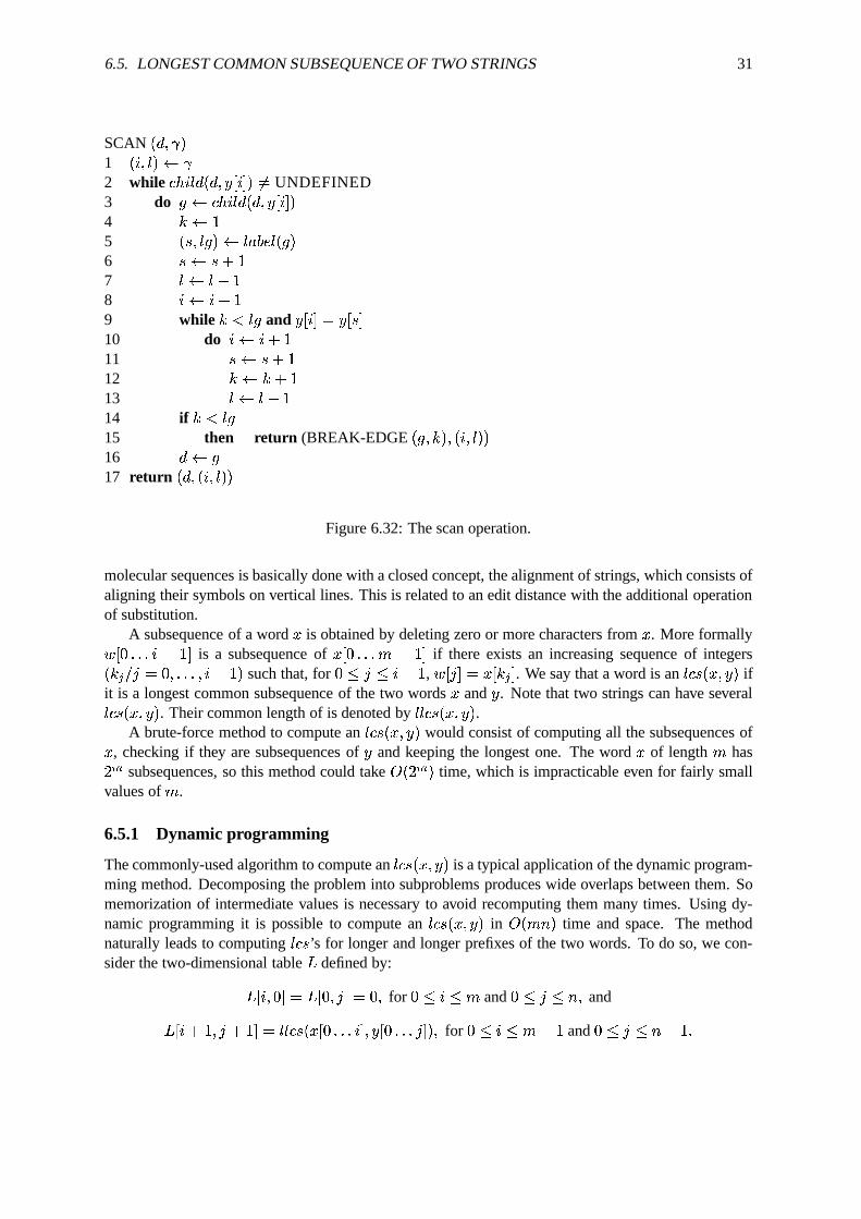
Figure 6.32: The scan operation.
molecular sequences is basically done with a closed concept, the alignment of strings, which consists ofaligning their symbols on vertical lines. This is related to an edit distance with the additional operationof substitution.
A subsequence of a word � is obtained by deleting zero or more characters from � . More formally� , ������� � � � / is a subsequence of � , ������� � � � / if there exists an increasing sequence of integers ��� � � (� ������� � � � � � such that, for � � � � � ��� , � , � /�(+� , ��� / . We say that a word is an �"�$#%����&�'� ifit is a longest common subsequence of the two words � and � . Note that two strings can have several�"�$#%����&�'� . Their common length of is denoted by ���"�$#�����&�9� .
A brute-force method to compute an �"�$#%����&�'� would consist of computing all the subsequences of� , checking if they are subsequences of � and keeping the longest one. The word � of length � has� � subsequences, so this method could take 12 � � � time, which is impracticable even for fairly smallvalues of � .
6.5.1 Dynamic programming
The commonly-used algorithm to compute an �"��#�����&�9� is a typical application of the dynamic program-ming method. Decomposing the problem into subproblems produces wide overlaps between them. Somemorization of intermediate values is necessary to avoid recomputing them many times. Using dy-namic programming it is possible to compute an �"��#�����&�9� in 12������ time and space. The methodnaturally leads to computing ���$# ’s for longer and longer prefixes of the two words. To do so, we con-sider the two-dimensional table * defined by:
*-, � � ��/ (+* , � � � / (� � for � � ��� � and � � � � � � and
* , � � � � � � � /0( ���"�$#��� , ������� � / �&�0, ������� � /�� � for ��� ��� � ��� and � � � � � ��� �

32 CHAPTER 6. PATTERN MATCHING AND TEXT COMPRESSION ALGORITHMS
int LCS(char *x, char *y, int m, int n, int L[YSIZE][YSIZE]) {int i, j;
for (i=0; i <= m; i++) L[i][0]=0;for (j=0; j <= n; j++) L[0][j]=0;
for (i=0; i < m; i++)for (j=0; j < n; j++)
if (x[i] == y[j]) L[i+1][j+1]=L[i][j]+1;else L[i+1][j+1]=MAX(L[i+1][j], L[i][j+1]);
return L[m][n];}
Figure 6.33: Dynamic programming algorithm to compute ���"�$#�����&�9� (+*-, �.�&�0/ .
char *TRACE(char *x, char *y, int m, int n, int L[YSIZE][YSIZE]) {int i, j, l;char z[YSIZE];
i=m; j=n; l=L[m][n];z[l--]=’\0’;while (i > 0 && j > 0) {
if (L[i][j] == L[i-1][j-1]+1 && x[i-1] == y[j-1]) {z[l--]=x[i-1];i--; j--;
}else if (L[i-1][j] > L[i][j-1]) i--;else j--;
}return(z);}
Figure 6.34: Production of an �"�$#%����&�'� .
Computing �"���$#�����&�9� (+* , �.�&�0/ relies on a basic observation that yields the simple recurrence relation( � � � � � , ��� � � � ):
* , � � � � � � � /0(�* , ��� � / � � if � , � /0( � , � / �3����8"*-, � � � � � / ��*-, � � � � � /�� otherwise.
The relation is used by the algorithm of Figure 6.33 to compute all the values from *-, � � ��/ to *-, �.�&�0/ .The computation takes 15������ time and space. It is afterward possible to trace back a path from * , �.�&�0/to exhibit an ���$#�����&�9� (see Figure 6.34).

6.5. LONGEST COMMON SUBSEQUENCE OF TWO STRINGS 33
int LLCS(char *x, char *y, int m, int n, int *L) {int i, j, last;
for (j=0; j <= n; j++) L[j]=0;for (i=0; i < m; i++) {
last=0;for (j=0; j < n; j++)
if (last > L[j+1]) L[j+1]=last;else if (last < L[j+1]) last=L[j+1];else if (x[i] == y[j]) {
L[j+1]++;last++;
}}return L[n];}
Figure 6.35: 12"35476 ��.�&���&� -space algorithm to compute �"�"��#�����&�9� .
Example 6.12:The value *-, ��� � / ( ! is �"���$#�����&�9� for � ( AGCGA and ��( CAGATAGAG. String AGGA is an lcs of �and � .
� C A G A T A G A G� 0 1 2 3 4 5 6 7 8 9A 0 0 0 0 0 0 0 0 0 0 0
G 1 0 0 1 1 1 1 1 1 1 1
C 2 0 0 1 2 2 2 2 2 2 2
G 3 0 1 1 2 2 2 2 2 2 2
A 4 0 1 1 2 2 2 2 3 3 3
5 0 1 2 2 3 3 3 3 4 4
6.5.2 Reducing the space: Hirschberg algorithm
If only the length of an �"�$#%����&�'� is required, it is easy to see that only one row (or one column) of thetable * needs to be stored during the computation. The space complexity becomes 12 min ��.�&���&� as itcan be checked on the algorithm of Figure 6.35. Indeed, the Hirschberg algorithm computes an �"�$#�����&�9�in linear space and not only the value �"���$#�����&�9� . The computation uses the algorithm of Figure 6.35.
Let us define:
* : , ���&�0/0( * : , �.� � / (� � for ��� ��� � and � � � � � � and
* : , � � � �&� � � /0( ���"�$#�&�� , � ����� � ��� /���
� ��0, � ������� ��� /���
� for � ����� � ��� and ��� � � � ��� �

34 CHAPTER 6. PATTERN MATCHING AND TEXT COMPRESSION ALGORITHMS
void LLCS_REVERSE(char *x, char *y, int a, int m, int n, int *Lstar) {int i, j, last;
for (j=0; j <= n; j++) Lstar[j]=0;for (i=m-1; i >= a; i--) {
last=0;for (j=n-1; j >= 0; j--)
if (last > Lstar[n-j]) Lstar[n-j]=last;else if (last < Lstar[n-j]) last=Lstar[n-j];else if (x[i] == y[j]) {Lstar[n-j]++;last++;
}}}
Figure 6.36: Computation of *;: .
and � � �)( 3����
=������� *-, ��� � / � * : , � � ���&� � � / �
where the word � �
is the reverse (or mirror image) of the word � . The algorithm of Figure 6.36compute the table * : . The following property is the key observation to compute an �"��#�����&�9� in linearspace:
for ��� � � �.�� � �)(+* , �.�&�0/ �
In the algorithm shown in Figure 6.37 the integer � is chosen as � � � . After * , ��� � / and * : , � � ���&� � � /( � � � � � ) are computed, the algorithm finds an integer
�such that * , ��� � /�� * : , � � ���&� � � / (
*-, �.�&�0/ . Then, recursively, it computes an ���$#��� , ������� � / �&�0, ������� � /�� and an �"�$#%�� , � � � ����� � � � / �&� , ���
����� � � � /�� , and concatenate them to get an �"�$#%����&�'� .The running time of the Hirschberg algorithm is still 12������ but the amount of space required for
the computation becomes 12"324768��.�&���&� instead of being quadratic as in Section 6.5.1.
6.6 Approximate string matching
Approximate string matching is the problem of finding all approximate occurrences of a pattern � oflength � in a text � of length � . Approximate occurrences of � are segments of � that are close to �according to a specific distance: the distance between segments and � must be not greater than a giveninteger
�. We consider two distances in this section, the Hamming distance and the Levenshtein
distance.With the Hamming distance, the problem is also known as approximate string matching with
�
mismatches. With the Levenshtein distance (or edit distance), the problem is known as approximatestring matching with
�differences.
The Hamming distance between two words � � and � � of the same length counts the number ofpositions with different characters. The Levenshtein distance between two words � � and � � (not nec-essarily of the same length) is the minimal number of differences between the two words. A differenceis one of the following operations:
� a substitution: a character of � � corresponds to a different character in � � ,

6.6. APPROXIMATE STRING MATCHING 35
char *HIRSCHBERG(char *x, char *y, int m, int n) {int i, j, k, M;static char z[YSIZE];static int L[YSIZE], Lstar[YSIZE];static int count=0;
if (m == 0) z[count]=’\0’;else if (m == 1) {
for (i=0; i < n; i++)if (x[0] == y[i]) {
z[count++]=x[0];z[count]=’\0’;return(z);
}z[count]=’\0’;
}else {
i=m/2;LLCS(x, y, i, n, L);LLCS_REVERSE(x, y, i, m, n, Lstar);k=n;M=L[n]+Lstar[0];for (j=n-1; j >= 0; j--)
if (L[j]+Lstar[n-j] >= M) {M=L[j]+Lstar[n-j];k=j;
}HIRSCHBERG(x, y, i, k);HIRSCHBERG(x+i, y+k, m-i, n-k);z[count]=’\0’;
}return(z);}
Figure 6.37: 12"324 68��.�&���&� -space computation of �"�$#%����&�'� .

36 CHAPTER 6. PATTERN MATCHING AND TEXT COMPRESSION ALGORITHMS
��
� , ��/� , ������� � /� , ������� � /
�
� (�� ( �� (��
� ( � � �
1
0
1
0
< =?
......
......
Figure 6.38: Meaning of vector < =? .
� an insertion: a character of � � corresponds to no character in � � ,� a deletion: a character of � � corresponds to no character in � � .The Shift-Or algorithm of the next section is a method that is both very fast in practice and very
easy to implement. It solves the two above problems. We initially describe the method for the exactstring-matching problem and then we show how it can handle the cases of
�mismatches and of
�
insertions, deletions, or substitutions. The method is flexible enough to be adapted to a wide range ofsimilar approximate matching problems.
6.6.1 Shift-Or algorithm
We first present an algorithm to solve the exact string-matching problem using a technique differentfrom those developed in Section 6.2, but which extends to the approximate string-matching problem.
Let <>= be a bit array of size � . Vector <>=? is the value of the entire array <�= after text character � , � /has been processed (see Figure 6.38). It contains information about all matches of prefixes of � that endat position � in the text ( � � � � � ��� ):
< =? , � / (�� if � , ������� � /0(+�0, � � � ����� � / ��
otherwise.
Therefore, < =? , � � � / ( � is equivalent to say that an (exact) occurrence of the pattern � ends at position� in � .
The vector <>=? can be computed after <>=? � � by the following recurrence relation:
< =? , � / (�� if < =? � � , � � � /0(� and � , � / ( �0, � / ��
otherwise,
and
< =? , ��/8(�� if � , ��/ ( � , � / ��
otherwise.
The transition from < =? � � to < =? can be computed very fast as follows. For each � � �, let ��� be a
bit array of size � defined by:
for � � � � � ��� � ���%, � / (� iff � , � /8(+���
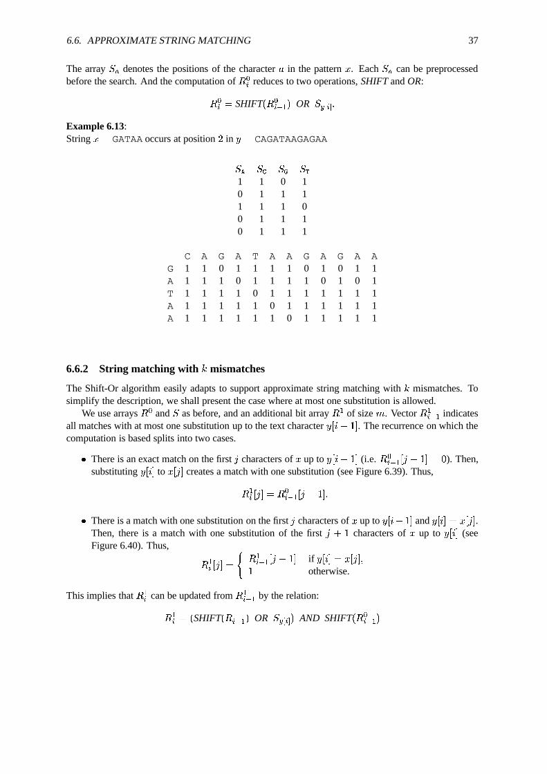
6.6. APPROXIMATE STRING MATCHING 37
The array ��� denotes the positions of the character � in the pattern � . Each � � can be preprocessedbefore the search. And the computation of < =? reduces to two operations, SHIFT and OR:
< =? ( SHIFT "< =? � � � OR � ��� ?�� �
Example 6.13:String � ( GATAA occurs at position � in �2( CAGATAAGAGAA
��� �� �� ���1 1 0 10 1 1 11 1 1 00 1 1 10 1 1 1
C A G A T A A G A G A AG 1 1 0 1 1 1 1 0 1 0 1 1A 1 1 1 0 1 1 1 1 0 1 0 1T 1 1 1 1 0 1 1 1 1 1 1 1A 1 1 1 1 1 0 1 1 1 1 1 1A 1 1 1 1 1 1 0 1 1 1 1 1
6.6.2 String matching with � mismatches
The Shift-Or algorithm easily adapts to support approximate string matching with�
mismatches. Tosimplify the description, we shall present the case where at most one substitution is allowed.
We use arrays <>= and � as before, and an additional bit array < � of size � . Vector < �? � � indicatesall matches with at most one substitution up to the text character � , � � � / . The recurrence on which thecomputation is based splits into two cases.
� There is an exact match on the first�
characters of � up to � , � ��� / (i.e. <�=? � � , ����� / (� ). Then,substituting � , � / to � , � / creates a match with one substitution (see Figure 6.39). Thus,
<�? , � /0(+< =? � � , ����� / �
� There is a match with one substitution on the first�
characters of � up to � , � � � / and � , � /0( � , � / .Then, there is a match with one substitution of the first
���
characters of � up to � , � / (seeFigure 6.40). Thus,
<�? , � /0(
�< �? � � , ����� / if � , � /0( � , � / ��
otherwise.
This implies that < �? can be updated from < �? � � by the relation:
<�? ( SHIFT "<
�? � � � OR � ��� ?�� � AND SHIFT "< =? � � �

38 CHAPTER 6. PATTERN MATCHING AND TEXT COMPRESSION ALGORITHMS
�
�i -1 i
j -1 j
Figure 6.39: If < =? � � , ����� /0(� then < �? , � / ( � .
�
�
�i -1 i
j -1 j
Figure 6.40: < �? , � / ( < �? � � , ����� / if � , � /0( � , � / .
Example 6.14:String � ( GATAA occurs at positions � and � in � ( CAGATAAGAGAA with no more than onemismatch.
C A G A T A A G A G A AG 0 0 0 0 0 0 0 0 0 0 0 0A 1 0 1 0 1 0 0 1 0 1 0 0T 1 1 1 1 0 1 1 1 1 0 1 0A 1 1 1 1 1 0 1 1 1 1 0 1A 1 1 1 1 1 1 0 1 1 1 1 0
6.6.3 String matching with � differences
We show in this section how to adapt the Shift-Or algorithm to the case of only one insertion, and thento the case of only one deletion. The method is based on the following elements.
One insertion allowed: here, vector < �? � � indicates all matches with at most one insertion up to textcharacter �0, � ��� / .< �? � � , � � � /-( � if the first
�characters of � ( � , ������� � � � / ) match
�symbols of the last
���
textcharacters up to �0, � ��� / .Array < = is maintained as before, and we show how to maintain array < � . Two cases can arise:
� There is an exact match on the first�
characters of � ( � , ������� � � � / ) up to � , � � � / . Then inserting� , � / creates a match with one insertion up to � , � / (see Figure 6.41). Thus
<�? , � /0(+< =? � � , ����� / �

6.6. APPROXIMATE STRING MATCHING 39
�
�i -1 i
j -1 j
Figure 6.41: If < =? � � , ����� /0(� then < �? , � / ( � .
�
�
�i -1 i
j -1 j
Figure 6.42: < �? , � / ( < �? � � , ����� / if � , � /0( � , � / .
� There is a match with one insertion on the�
first characters of � up to � , � � � / . Then if �0, � /0( � , � /there is a match with one insertion on the first
���
characters of � up to �0, � / (see Figure 6.42).Thus,
<�? , � /0(
�< �? � � , ����� / if � , � /0( � , � / ��
otherwise.
The above shows that < �? can be updated from < �? � � with the formula:
<�? ( SHIFT "<
�? � � � OR � ��� ?�� � AND < =? � � �Example 6.15:GATAAG is an occurrence of ��( GATAA with one insertion in �2( CAGATAAGAGAA
C A G A T A A G A G A AG 1 1 1 0 1 1 1 1 0 1 0 1A 1 1 1 1 0 1 1 1 1 0 1 0T 1 1 1 1 1 0 1 1 1 1 1 1A 1 1 1 1 1 1 0 1 1 1 1 1A 1 1 1 1 1 1 1 0 1 1 1 1
One deletion allowed: We assume here that < �? � � indicates all possible matches with at most onedeletion up to � , � ��� / . As in previous problems, two cases arise:
� There is an exact match on the first���
characters of � ( � , ������� � / ) up to �0, � / (i.e. < =? , � / ( � ).Then, deleting � , � / creates a match with one deletion (see Figure 6.43). Thus,
<�? , � /8(+< =? , � / �
40 CHAPTER 6. PATTERN MATCHING AND TEXT COMPRESSION ALGORITHMS
�
�i -1 i
j -1 j
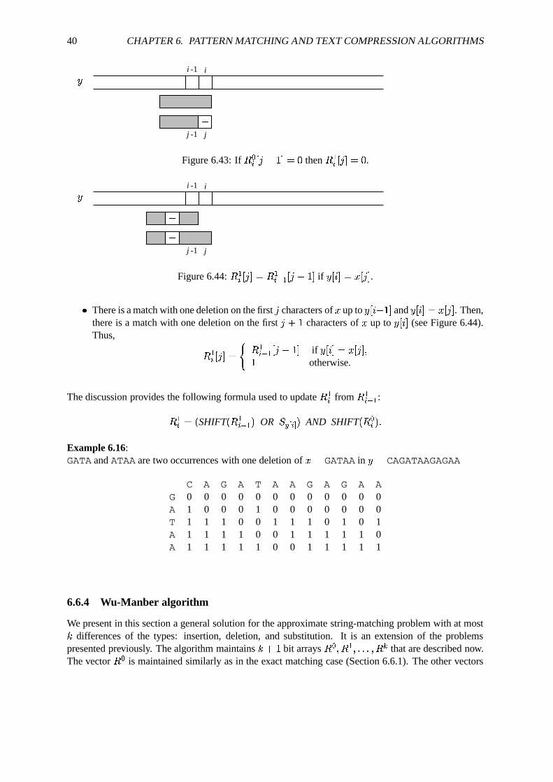
Figure 6.43: If < =? , � � � /0(� then < �? , � /0(� .
��
�i -1 i
j -1 j
Figure 6.44: < �? , � / ( < �? � � , ����� / if � , � /0( � , � / .
� There is a match with one deletion on the first�
characters of � up to � , � ��� / and � , � /0(+� , � / . Then,there is a match with one deletion on the first
���
characters of � up to � , � / (see Figure 6.44).Thus,
<�? , � /0(
�< �? � � , ����� / if � , � /0( � , � / ��
otherwise.
The discussion provides the following formula used to update < �? from < �? � � :
<�? ( SHIFT "<
�? � � � OR � ��� ?�� � AND SHIFT "< =? � �
Example 6.16:GATA and ATAA are two occurrences with one deletion of � ( GATAA in � ( CAGATAAGAGAA
C A G A T A A G A G A AG 0 0 0 0 0 0 0 0 0 0 0 0A 1 0 0 0 1 0 0 0 0 0 0 0T 1 1 1 0 0 1 1 1 0 1 0 1A 1 1 1 1 0 0 1 1 1 1 1 0A 1 1 1 1 1 0 0 1 1 1 1 1
6.6.4 Wu-Manber algorithm
We present in this section a general solution for the approximate string-matching problem with at most�
differences of the types: insertion, deletion, and substitution. It is an extension of the problemspresented previously. The algorithm maintains
���
bit arrays < = ��< � ������� ��< � that are described now.The vector < = is maintained similarly as in the exact matching case (Section 6.6.1). The other vectors

6.7. TEXT COMPRESSION 41
are computed with the formula (� � � � �
):
<�
? ( SHIFT "<�
? � � � OR � ��� ?�� �AND SHIFT "<
� � �? �AND SHIFT "<
� � �? � � �AND <
� � �? � � �which can be rewritten into:
<�
? ( SHIFT "<�
? � � � OR � ��� ?�� �AND SHIFT "<
� � �? AND <� � �? � � �
AND <� � �? � � �
Example 6.17:� ( GATAA and � ( CAGATAAGAGAA and
� ( � The following output: 5, 6, 7, and 11 correspondsto the segments: GATA, GATAA, GATAAG, and GAGAA which approximate the pattern GATAA with nomore than one difference.
C A G A T A A G A G A AG 0 0 0 0 0 0 0 0 0 0 0 0A 1 0 0 0 0 0 0 0 0 0 0 0T 1 1 1 0 0 0 1 1 0 0 0 0A 1 1 1 1 0 0 0 1 1 1 0 0A 1 1 1 1 1 0 0 0 1 1 1 0
The method, called the Wu-Manber algorithm, is implemented in Figure 6.45. It assumes that thelength of the pattern is no more than the size of the memory-word of the machine, which is often thecase in applications.
The preprocessing phase of the algorithm takes 12 �0� �� � � memory space, and runs in time
12 �0� �� � . The time complexity of its searching phase is 12 � ��� .
6.7 Text compression
In this section we are interested in algorithms that compress texts. Compression serves both to savestorage space and to save transmission time. We shall assume that the uncompressed text is stored in afile. The aim of compression algorithms is to produce another file containing the compressed versionof the same text. Methods in this section work with no loss of information, so that decompressing thecompressed text restores exactly the original text.
We apply two strategies to design the algorithms. The first strategy is a statistical method that takesinto account the frequencies of symbols to build a uniquely decipherable code optimal with respectto the compression. The code contains new codewords for the symbols occurring in the text. In thismethod fixed-length blocks of bits are encoded by different codewords. A contrario the second strategyencodes variable-length segments of the text. To put it simply, the algorithm, while scanning the text,replaces some already read segments by just a pointer to their first occurrences.
6.7.1 Huffman coding
The Huffman method is an optimal statistical coding. It transforms the original code used for charactersof the text (ASCII code on
�bits, for instance). Coding the text is just replacing each symbol (more

42 CHAPTER 6. PATTERN MATCHING AND TEXT COMPRESSION ALGORITHMS
void WM(char *y, char *x, int n, int m, int k) {unsigned int j, last1, last2, lim, mask, S[ASIZE], R[KSIZE];int i;
/* Preprocessing */for (i=0; i < ASIZE; i++) S[i]=˜0;lim=0;for (i=0, j=1; i < m; i++, j<<=1) {
S[x[i]]&=˜j;lim|=j;
}lim=˜(lim>>1);R[0]=˜0;for (j=1; j <= k; j++) R[j]=R[j-1]>>1;
/* Search */for (i=0; i < n; i++) {
last1=R[0];mask=S[y[i]];R[0]=(R[0]<<1)|mask;for (j=1; j <= k; j++) {
last2=R[j];R[j]=((R[j]<<1)|mask)&((last1&R[j-1])<<1)&last1;last1=last2;
}if (R[k] < lim) OUTPUT(i);
}}
Figure 6.45: Wu-Manber approximate string-matching algorithm.

6.7. TEXT COMPRESSION 43
COUNT fin �1 for each character � � �
2 do freq "�'� � �3 while not end of file fin and � is the next symbol4 do freq "�'� � freq "�'� � �5 freq END � � �
Figure 6.46: Counts the character frequencies.
exactly each occurrence of it) by its new codeword. The method works for any length of blocks (notonly
�bits), but the running time grows exponentially with the length. In the following, we assume that
symbols are originally encoded on�
bits to simplify the description.The Huffman algorithm uses the notion of prefix code. A prefix code is a set of words containing
no word that is a prefix of another word of the set. The advantage of such a code is that decoding isimmediate. Moreover, it can be proved that this type of code does not weaken the compression.
A prefix code on the binary alphabet � � � � � can be represented by a trie (see Section 6.2.6) that is abinary tree. In the present method codes are complete: they correspond to complete tries (internal nodeshave exactly two children). The leaves are labeled by the original characters, edges are labeled by 0 or1, and labels of branches are the words of the code. The condition on the code implies that codewordsare identified with leaves only. We adopt the convention that, from a internal node, the edge to its leftchild is labeled by 0, and the edge to its right child is labeled by 1.
In the model where characters of the text are given new codewords, the Huffman algorithm builds acode that is optimal in the sense that the compression is the best possible (the length of the compressedtext is minimum). The code depends on the text, and more precisely on the frequencies of each char-acter in the uncompressed text. The more frequent characters are given short codewords while the lessfrequent symbols have longer codewords.
Encoding
The coding algorithm is composed of three steps: count of character frequencies, construction of theprefix code, encoding of the text.
The first step consists of counting the number of occurrences of each character in the original text(see Figure 6.46). We use a special end marker (denoted by END), which (virtually) appears only onceat the end of the text. It is possible to skip this first step if fixed statistics on the alphabet are used. Inthis case the method is optimal according to the statistics, but not necessarily for the specific text.
The second step of the algorithm builds the tree of a prefix code using the character frequencyfreq "�'� of each character � in the following way:
� create a one-node tree for each character � , setting � � � � � $� &�;( freq "�'� and �"� � ���&� &�)(+� ,� repeat
– Extract the two least weighted trees � and � ,– Create a new tree �� having left subtree � , right subtree � , and weight � � � � � $� ���� (� � � � � $� � � � � � � � � $� � �
� until only one tree remains.

44 CHAPTER 6. PATTERN MATCHING AND TEXT COMPRESSION ALGORITHMS
BUILD-TREE1 for each � � � � ������� �2 do if freq "�'� �(�3 then create a new node 4 � � � � � $� &��� freq "� �5 ��� � ���&� �� � �6 �"�"� � � � # � list of all the nodes in increasing order of weight7 �� � � # � empty list8 while LENGTH "�"� ���%��� #�� + LENGTH "� � � #���� �9 do "� �& � � extract the two nodes of smallest weight (among the two nodes at the beginning
of �"� ���%��� # and the two nodes at the beginning of �� � � # )10 create a new node 11 � � � � � �� ���� � � � � � $"� � � � � � � � $� �12 � ��� $� �� � �13 � � � �� �� � 14 insert at the end of �� � � #15 # � � � � # � � � ���16 return
Figure 6.47: Builds the coding tree.
The tree is constructed by the algorithm BUILD-TREE in Figure 6.47. The implementation uses twolinear lists. The first list contains the leaves of the future tree associated each with a symbol. The list issorted in the increasing order of the weight of the leaves (symbol frequency of symbols). The secondlist contains the newly created trees. Extracting the two least weighted trees consists of extracting thetwo least weighted trees among the two first trees of the list of leaves and the two first trees of the listof created trees. Each new tree is inserted at the end of the list of the trees. The only tree remaining atthe end of the procedure is the coding tree.
After the coding tree is built, it is possible to recover the codewords associated with characters by asimple depth-first-search of the tree (see Figure 6.48); ��� ��$� � "� � is then the binary code associatedwith the character � .
In the third step, the original text is encoded. Since the code depends on the original text, in orderto be able to decode the compressed text, the coding tree and the original codewords of symbols mustbe stored with the compressed text. These information are placed in a header of the compressed file, tobe read at decoding time just before the compressed text. The header is made via a depth-first traversalof the tree. Each time an internal node is encountered a 0 is produced. When a leaf is encountered a 1 isproduced followed by the original code of the corresponding character on 9 bits (so that the end markercan be equal to 256 if all the characters appear in the original text). This part of the encoding algorithmis shown in Figure 6.49.
After the header of the compressed file is computed, the encoding of the original text is realized bythe algorithm of Figure 6.50.
A complete implementation of the Huffman algorithm, composed of the three steps described above,is given in Figure 6.51.

6.7. TEXT COMPRESSION 45
BUILD-CODE � ��� ��� � � �1 if is not a leaf2 then ��� � , � �$� � � / � �3 BUILD-CODE "� ��� $� &� ��� ��� � � � � �4 &�$� � , � �$� �% � / � �5 BUILD-CODE � � � � �� �� ��� �$� � � � � �6 else ��� ��$� � "��� � ���&� ��&� � ��� � , ������� � �$� � � ��� /
Figure 6.48: Builds the character codes from coding tree.
CODE-TREE fout �& ��1 if is not a leaf2 then write a 0 in the file fout3 CODE-TREE fout ��� ��� $� ��&�4 CODE-TREE fout �& � � � �� ��&�5 else write a 1 in the file fout6 write the original code of �"� � � �&� &� in the file fout
Figure 6.49: Memorizes the coding tree in the compressed file.
CODE-TEXT fin � fout �1 while not end of file fin and � is the next symbol2 do write � � ��$�-�� �"�'� in the file fout3 write ��� %���-�� � END � in the file fout
Figure 6.50: Encodes the characters in the compressed file.
CODING fin � fout �1 COUNT fin �3 � BUILD-TREE3 BUILD-CODE � � � �4 CODE-TREE fout �& &�5 CODE-TEXT fin � fout �
Figure 6.51: Complete function for Huffman coding.

46 CHAPTER 6. PATTERN MATCHING AND TEXT COMPRESSION ALGORITHMS
Example 6.18:�2( � � � � � � � � � � � �Length of �2( � � � � ( ��� bits (assuming an 8-bit code)
Character frequencies:A C G T END7 1 3 1 1
Different steps during the construction of the coding tree:
1 1 1 3 7 1 2 3 7
C T END G A END 1 1 G A
C T
3 3 7 6 7
1 2 G A 3 3 A
END 1 1 1 2 G
C T END 1 1
C T
13
6 7
3 3 A
1 2 G
END 1 1
C T
character codewords:A C G T END1 0010 01 0011 000
Encoded tree: 0001binary(END,9)01binary(C,9)1 binary(T,9)1binary(G,9)1binary(A,9),which produces a header of length � ! bits:0001 100000000 01 001000011 1 001010100 1 001000111 1 001000001
Encoded text: 0010 1 01 1 0011 1 1 01 1 01 1 1 000,of length � ! bits
Total length of the compressed file: � �bits
The construction of the tree takes 15 � ����� ��� time if the sorting of the list of the leaves is imple-mented efficiently. The rest of the encoding process runs in time linear in the sum of the sizes of theoriginal and compressed texts.

6.7. TEXT COMPRESSION 47
REBUILD-TREE fin �& ��1
�� read a bit from the file fin
2 if� ( � /* leaf */
3 then �"� � �� �� � NIL4 � � � �� �� � NIL5 �"� � � � � �� � symbol corresponding to the � next bits in the file fin6 else create a new node �7 � ��� $� &� � �8 REBUILD-TREE fin ��� �9 create a new node 10 � � � �� �� � 11 REBUILD-TREE fin �& �
Figure 6.52: Rebuilds the tree read from the compressed file.
DECODE-TEXT fin � fout �& ���� &�1 � ����� 2 while �"� � ���&� &� �( END3 do if is a leaf4 then write �"� � � � � �� in the file fout5 � ����� 6 else
�� read a bit from the file fin
7 if� ( �
8 then � � � � $� &�9 else � � ��� $� &�
Figure 6.53: Reads the compressed text and produces the uncompressed text.
Decoding
Decoding a file containing a text compressed by Huffman algorithm is a mere programming exercise.First the coding tree is rebuilt by the algorithm of Figure 6.52. Then, the uncompressed text is recoveredby parsing the compressed text with the coding tree. The process begins at the root of the coding tree,and follows a left edge when a � is read or a right edge when a
�is read. When a leaf is encountered,
the corresponding character (in fact the original codeword of it) is produced and the parsing phaseresumes at the root of the tree. The parsing ends when the codeword of the end marker is read. Animplementation of the decoding of the text is presented in Figure 6.53.
The complete decoding program is given in Figure 6.54. It calls the preceding functions. Therunning time of the decoding program is linear in the sum of the sizes of the texts it manipulates.

48 CHAPTER 6. PATTERN MATCHING AND TEXT COMPRESSION ALGORITHMS
DECODING fin � fout �1 create a new node ��� 2 REBUILD-TREE fin �& ���� ��3 DECODE-TEXT fin � fout �& ���� &�
Figure 6.54: Complete function for decoding.
6.7.2 LZW Compression
Ziv and Lempel designed a compression method using encoding segments. These segments are storedin a dictionary that is built during the compression process. When a segment of the dictionary is en-countered later while scanning the original text it is substituted by its index in the dictionary. In themodel where portions of the text are replaced by pointers on previous occurrences, the Ziv-Lempelcompression scheme can be proved to be asymptotically optimal (on large enough texts satisfying goodconditions on the probability distribution of symbols).
The dictionary is the central point of the algorithm. It has the property of being prefix-closed(every prefix of a word of the dictionary is in the dictionary), so that it can be implemented as a tree.Furthermore, a hashing technique makes its implementation efficient. The version described in thissection is called the Lempel-Ziv-Welch method after several improvements introduced by Welch. Thealgorithm is implemented by the compress command existing under the UNIX operating system.
Compression method
We describe the scheme of the compression method. The dictionary is initialized with all the charactersof the alphabet. The current situation is when we have just read a segment � in the text. Let � be thenext symbol (just following � ). Then we proceed as follows:
� If � � is not in the dictionary, we write the index of � to the output file, and add �-� to thedictionary. We then reset � to � and process the next symbol (following � ).
� If �-� is in the dictionary we process the next symbol, with segment � � instead of � .
Initially, the segment � is set to the first symbol of the source text.
Example 6.19:�2( � � � � � � � � � � �

6.7. TEXT COMPRESSION 49
C A G T A A G A G A A � written added�
C 67 CA, 257�
A 65 AG, 258�
G 71 GT, 259�
T 84 TA, 260�
A 65 AA, 261�
A�
AG 258 AGA, 262�
A�
AG�
AGA 262 AGAA, 262�
A65
256
Decompression method
The decompression method is symmetric to the compression algorithm. The dictionary is recoveredwhile the decompression process runs. It is basically done in this way:
� read a code � in the compressed file,� write in the output file the segment � which has index � in the dictionary,� add to the dictionary the word � � where � is the first letter of the next segment.
In this scheme, a problem occurs if the next segment is the word which is being built. This arises onlyif the text contains a segment ��� ��� �%� for which ��� belongs to the dictionary but ��� � does not. Duringthe compression process the index of ��� is written into the compressed file, and ��� � is added to thedictionary. Next, � � � is read and its index is written into the file. During the decompression processthe index of � � � is read while the word ��� has not been completed yet: the segment � � � is not alreadyin the dictionary. However, since this is the unique case where the situation arises, the segment � � � isrecovered taking the last segment ��� added to the dictionary concatenated with its first letter � .Example 6.20:decoding: 67, 65, 71, 84, 65, 258, 262, 65, 256
read written added67 C65 A CA, 25771 G AG, 25884 T GT, 25965 A TA, 260
258 AG AA, 261262 AGA AGA, 26265 A AGAA, 263
256

50 CHAPTER 6. PATTERN MATCHING AND TEXT COMPRESSION ALGORITHMS
COMPRESS fin � fout �1 ��� ��� � ���2 for each character � � �
3 do ������� � ������� � �4 HASH-INSERT �� � ��� ������� ����� &�&�5 ��� ��� � � ����� � �6 HASH-INSERT �� � ��� � END ��������� ��&�7 � � ���8 while not end of file fin9 do � � next character of fin10 � � HASH-SEARCH �� � ����� �&�11 if �>( NIL12 then write � � �� �0� on
�� ����� "� ����� &� bits in fout
13 � ����� � ������� � �14 HASH-INSERT �� � ����������� ��� &�&�15 � � HASH-SEARCH �� � � � ��� �&�16 else � � �17 write � on
�� ������"������� �� bits in fout
18 write ��� %�% HASH-SEARCH �� � ��� � END �&� in�� �����0"��� ��� &� bits in fout
Figure 6.55: LZW compression algorithm.
Implementation
For the compression algorithm shown in Figure 6.55, the dictionary is stored in a table � . The dictio-nary is implemented as a tree; each node � of the tree has the three following components:
� � � �$� $ �%� : a link to the parent node of � ,
� �"� � ���& �%� : a character,
� ��� %�% �%� : the code associated with � .
The tree is stored in table that is accessed with a hashing function. This provides a fast access to thechildren of a node. The procedure HASH-INSERT �� � �����������&� inserts a new node � in the dictionary� with ���% �$� $ �%� ( �����"� � � � ���2( � and ��� �� �%� ( � . The function HASH-SEARCH �� � ����� �&�returns the node � such that ���% �$� $ �%� ( � and ��� � ���& �%� ( � .
For the decompression algorithm, no hashing technique is necessary. Having the index of the nextsegment, a bottom-up walk in the trie implementing the dictionary produces the mirror image of thesegment. A stack is used to reverse it. We assume that the function # � � � "��� performs this specificwork for a code � . The bottom-up walk follows the parent links of the data structure. The functionfirst �� � gives the first character of the word � . These features are part of the decompression algorithmdisplayed in Figure 6.56.
The Ziv-Lempel compression and decompression algorithms run both in time linear in the sizesof the files provided a good hashing technique is chosen. Indeed, it is very fast in practice. Its mainadvantage compared to Huffman coding is that it captures long repeated segments in the source file.

6.7. TEXT COMPRESSION 51
UNCOMPRESS fin � fout �1 ��� ��� � ���2 for each character � � �
3 do ������� � ������� � �4 HASH-INSERT �� � ��� ������� ����� &�&�5 ��� ��� � � ����� � �6 HASH-INSERT �� � ��� � END ��������� ��&�7 � � first code on
���������"������� �� bits in fin
8 write # � � �0"�$� in fout9 � � first #� � � � "���&�10 repeat11 � next code on
�� ����� "������� �� in the fin
12 if � � ����� 13 then ������� � ������� � �14 ���% ��� �"������� �� � �15 �"� � ���&"������� �� � �16 write # � � � "��� � in fout17 � � 18 else � � first # � � �0 ��&�19 if � �( END20 then ��� ��� � � ����� � �21 ���% �$� $"��� ��� &��� �22 �"� � � �&"� ����� &� � �23 write #� � � � �� in fout17 � � 24 else exit25 forever
Figure 6.56: LZW decompression algorithm.

52 CHAPTER 6. PATTERN MATCHING AND TEXT COMPRESSION ALGORITHMS
Source texts French C sources Alphabet RandomSizes in bytes 62816 684497 530000 70000Huffman 53.27% 62.10% 72.65% 55.58%Ziv-Lempel 41.46% 34.16% 2.13% 63.60%Factor 47.43% 31.86% 0.09% 73.74%
Figure 6.57: Sizes of texts compressed with three algorithms.
6.7.3 Experimental results
The table of Figure 6.57 contains a sample of experimental results showing the behavior of com-pression algorithms on different types of texts. The table is extracted from (Zipstein, 1992).
The source files are: French text, C sources, Alphabet, and Random. Alphabet is a file containga repetition of the line abc...zABC...Z. Random is a file where the symbols have been generatedrandomly, all with the same probability and independently of each others.
The compression algorithms reported in the table are: the Huffman algorithm of Section 6.7.1,the Ziv-Lempel algorithm of Section 6.7.2, and a third algorithm called Factor. This latter algorithmencodes segments of the source text as Ziv-Lempel algorithm does. But the segments are taken amongall segments already encountered in the text before the current position. The method gives usually bettercompression ratio but is more difficult to implement.
The table of Figure 6.57 gives in percentage the sizes of compressed files. Results obtained by Ziv-Lempel and Factor algorithms are similar. Huffman coding gives the best result for the Random file.Finally, experience shows that exact compression methods often reduce the size of data to 30%–50% oftheir original size.
6.8 Research Issues and Summary
The algorithm for string searching by hashing was introduced by Harrison (1971), and later fully ana-lyzed by Karp and Rabin (1987).
The linear-time string-matching algorithm of Knuth, Morris, and Pratt is from 1976. It can beproved that, during the search, a character of the text is compared to a character of the pattern no morethan ������� � � ��� � � (where
�is the golden ratio � � �
� � � � ). Simon (1993) gives an algorithm similarto the previous one but with a delay bounded by the size of the alphabet (of the pattern � ). Hancart(1993) proves that the delay of Simon’s algorithm is indeed no more than
�������� � � � � . He also proves
that this is optimal among algorithms searching the text through a window of size�.
Galil (1981) gives a general criterion to transform searching algorithms of that type into real-timealgorithm.
The Boyer-Moore algorithm was designed by Boyer and Moore (1977). The first proof on thelinearity of the algorithm when restricted to the search of the first occurrence of the pattern is in (Knuth,Morris and Pratt, 1977). Cole (1995) proves that the maximum number of symbol comparisons isbounded by ��� , and that this bound is tight.
Knuth, Morris, and Pratt (1977) consider a variant of the Boyer-Moore algorithm in which allprevious matches inside the current window are memorized. Each window configuration becomes thestate of what is called the Boyer-Moore automaton. It is still unknown whether the maximum numberof states of the automaton is polynomial or not.
Several variants of the Boyer-Moore algorithm avoid the quadratic behavior when searching for alloccurrences of the pattern. Among the more efficient in terms of the number of symbol comparisons

6.9. DEFINING TERMS 53
are: the algorithm of Apostolico and Giancarlo (1986), Turbo-BM algorithm by Crochemore et alii(1992) (the two algorithms are analyzed in Lecroq, 1995), and the algorithm of Colussi (1994).
The general bound on the expected time complexity of string matching is O( � � � ����� � � � � � � � ). Theprobabilistic analysis of a simplified version of the Boyer-Moore algorithm, similar to the Quick Searchalgorithm of Sunday (1990) described in the chapter, was studied by several authors.
String searching can be solved by a linear-time algorithm requiring only a constant amount ofmemory in addition to the pattern and the (window on the) text. This can be proved by differenttechniques presented in (Crochemore and Rytter, 1994).
It is known that any string searching algorithm, working with symbol comparisons, makes at least� ����
��� � � � comparisons in the worst case (see Cole et al. 1995). Some string searching algorithms
make less than ��� comparisons at search phase. The presently-known upper bound on the problem is� � �
��� � ���� �� � � � , but with a quadratic-time preprocessing step (Cole et al., 1995). With a linear-time
preprocessing step, the current upper bound is � ���� �
� � ��
�� � � � by Breslauer and Galil (1993).Except in few cases (patterns of length � , for example), lower and upper bound do not meet. So, theproblem of the exact complexity of string searching is open.
The Aho-Corasick algorithm is from (Aho and Corasick, 1975). It is implemented by the fgrepcommand under the UNIX operating system. Commentz-Walter (1979) has designed an extension ofthe Boyer-Moore algorithm to several patterns. It is fully described in (Aho, 1990).
On general alphabets the two-dimensional pattern matching can be solved in linear time while therunning time of the Bird/Baker algorithm has an additional ����� � factor. It is still unknown whether theproblem can be solved by an algorithm working simultaneously in linear time and using only a constantamount of memory space (see Crochemore et al., 1994).
The suffix tree construction of Section 6.4 is by McCreight (1976). Other data structures to representindexes on text files are: direct acyclic word graph (Blumer et al., 1985), suffix automata (Crochemore,1986), and suffix arrays (Myers and Manber, 1993). All these techniques are presented in (Crochemoreand Rytter, 1994). The data structures implement full indexes with standard operations while applica-tions sometimes need only incomplete indexes. The design of compact indexes is still unsolved.
Hirschberg (1975) presents the computation of the LCS in linear space. This is an important resultbecause the algorithm is classically run on large sequences. The quadratic time complexity of thealgorithm to compute the Levenshtein distance is a bottleneck in practical string comparison for thesame reason.
Approximate string searching is a lively domain of research. It includes for instance the notion ofregular expressions to represent sets of strings. Algorithms based on regular expression are commonlyfound in books related to compiling techniques. The algorithms of Section 6.6 are by Baeza-Yates andGonnet (1992), and Wu and Manber (1992).
The statistical compression algorithm of Huffman (1951) has a dynamic version where symbolcounting is done at coding time. The current coding tree is used to encode the next character and thenupdated. At decoding time a symmetrical process reconstructs the same tree, so the tree does not needto be stored with the compressed text. The command compact of UNIX implements this version.
Several variants of the Ziv and Lempel algorithm exist. The reader can refer to the book of Bell,Cleary, and Witten (1990) for a discussion on them. The book of Nelson (1992) presents practicalimplementations of various compression algorithms.
6.9 Defining Terms
Border: A word � � � : is a border of a word � � � : if � is both a prefix and a suffix of � (there existtwo words ��� � � � : such that � ( � � ( � � ). The common length of � and � is a period of � .
54 CHAPTER 6. PATTERN MATCHING AND TEXT COMPRESSION ALGORITHMS
Edit distance: The metric distance between two strings that counts the minimum number of insertionsand deletions of symbols to transform one string into the other.Hamming distance: The metric distance between two strings of same length that counts the number ofmismatches.Levenshtein distance: The metric distance between two strings that counts the minimum number ofinsertions, deletions, and substitutions of symbols to transform one string into the other.Occurrence: An occurrence of a word � � � : , of length � , appears in a word � � � : , of length � , atposition � if: for � � � � � � � , � , � /0( � , � � � / .Prefix: A word � � � : is a prefix of a word � � � : if � ( � � for some � � � : .Prefix code: Set of words such that no word of the set is a prefix of another word contained in the set.A prefix code is represented by a coding tree.Segment: A word � � � : is a segment of a word � � � : if � occurs in � (see occurrence), i.e.� ( � � � for two words ��� � � � : . ( � is also referred to as a factor or a subword of � )Subsequence: A word � � � : is a subsequence of a word � � � : if it is obtained form � by deletingzero or more symbols that need not be consecutive. ( � is sometimes referred to as a subword of � , witha possible confusion with the notion of segment).Suffix: A word � � � : is a suffix of a word � � � : if � ( � � for some � � � : .Suffix tree: Trie containing all the suffixes of a word.Trie: Tree in which edges are labeled by letters or words.
6.10 References
Aho, A.V. 1990. Algorithms for finding patterns in strings. In Handbook of Theoretical ComputerScience, vol. A, Algorithms and complexity, ed. J. van Leeuwen, p 255–300. Elsevier, Amsterdam.
Aho, A.V., and Corasick, M.J. 1975. Efficient string matching: an aid to bibliographic search. Comm.ACM. 18(6):333–340.
Baeza-Yates, R.A., and Gonnet, G.H. 1992. A new approach to text searching. Comm. ACM. 35(10):74–82.
Baker, T.P. 1978. A technique for extending rapid exact-match string matching to arrays of more thanone dimension. SIAM J. Comput. 7(4):533–541.
Bell, T.C., Cleary, J.G., and Witten, I.H. 1990. Text compression, Prentice Hall, Englewood Cliffs, NewJersey.
Bird, R.S. 1977. Two-dimensional pattern matching. Inf. Process. Lett. 6(5):168–170.
Blumer, A., Blumer, J., Ehrenfeucht, A., Haussler, D., Chen, M.T., and Seiferas, J. 1985. The smallestautomaton recognizing the subwords of a text. Theoret. Comput. Sci. 40:31–55.
Boyer, R.S., and Moore, J.S. 1977. A fast string searching algorithm. Comm. ACM. 20:762–772.
Breslauer, D., and Galil, Z. 1993. Efficient comparison based string matching. J. Complexity. 9(3):339–365.
Breslauer, D., Colussi, L., and Toniolo, L. 1993. Tight comparison bounds for the string prefix matchingproblem. Inf. Process. Lett. 47(1):51–57.
Cole, R. 1994. Tight bounds on the complexity of the Boyer-Moore pattern matching algorithm. SIAMJ. Comput. 23(5):1075–1091.

6.11. FURTHER INFORMATION 55
Cole, R., Hariharan, R., Zwick, U., and Paterson, M.S. 1995. Tighter lower bounds on the exact com-plexity of string matching. SIAM J. Comput. 24(1):30–45.
Colussi, L. 1994. Fastest pattern matching in strings. J. Algorithms. 16(2):163–189.
Crochemore, M. 1986. Transducers and repetitions. Theoret. Comput. Sci. 45(1):63–86.
Crochemore, M., and Rytter, W. 1994. Text Algorithms, Oxford University Press.
Galil, Z. 1981. String matching in real time. J. ACM. 28(1):134–149.
Hancart, C. 1993. On Simon’s string searching algorithm. Inf. Process. Lett. 47:95–99.
Hirschberg, D.S. 1975. A linear space algorithm for computing maximal common subsequences.Comm. ACM. 18(6):341–343.
Hume, A., Sunday, D.M. 1991. Fast string searching. Software – Practice and Experience. 21(11):1221–1248.
Karp, R.M., Rabin, M.O. 1987. Efficient randomized pattern-matching algorithms. IBM J. Res. Dev.31(2):249–260.
Knuth, D.E., Morris Jr, J.H., Pratt, V.R. 1977. Fast pattern matching in strings. SIAM J.Comput.6(1):323–350.
Lecroq, T. 1995. Experimental results on string-matching algorithms. Software - Practice & Experience25(7):727–765.
McCreight, E.M. 1976. A space-economical suffix tree construction algorithm. J. Algorithms. 23(2):262–272.
Manber, U., Myers, G. 1993. Suffix arrays: a new method for on-line string searches. SIAM J. Comput.22(5):935–948.
Nelson, M. 1992. The data compression book, M&T Books.
Simon, I. 1993. String matching algorithms and automata. In First American Workshop on StringProcessing, ed. Baeza-Yates and Ziviani, p 151–157. Universidade Federal de Minas Gerais.
Stephen, G.A. 1994. String searching algorithms, World Scientific Press.
Sunday, D.M. 1990. A very fast substring search algorithm. Comm. ACM. 33(8):132–142.
Welch, T. 1984. A technique for high-performance data compression. IEEE Computer. 17(6):8–19.
Wu, S., Manber, U. 1992. Fast text searching allowing errors. Comm. ACM. 35(10):83–91.
Zipstein, M. 1992. Data compression with factor automata. Theoret. Comput. Sci. 92(1):213–221.
Zhu, R.F., Takaoka, T. 1989. A technique for two-dimensional pattern matching. Comm. ACM.32(9):1110–1120.
6.11 Further Information
Problems and algorithms presented in the chapter are just a sample of questions related to patternmatching. They share the formal methods used to design solutions and efficient algorithms. A widerpanorama of algorithms on texts may be found in few books such as:
� Bell, T.C., Cleary, J.G., Witten, I.H. 1990. Text compression, Prentice Hall, Englewood Cliffs,New Jersey.
� Crochemore, M., Rytter, W. 1994. Text algorithms, Oxford University Press.

56 CHAPTER 6. PATTERN MATCHING AND TEXT COMPRESSION ALGORITHMS
� Nelson, M. 1992. The data compression book, M&T Books.� Stephen, G.A. 1994. String searching algorithms, World Scientific Press.
Research papers in pattern matching are disseminated in few journals, among which are: Commu-nications of the ACM, Journal of the ACM, Theoretical Computer Science, Algorithmica, Journal ofAlgorithms, SIAM Journal on Computing.
Finally, two main annual conferences present the latest advances of this field of research:
� Combinatorial Pattern Matching, which started in 1990 and was held in Paris (France), London(England), Tucson (Arizona), Padova (Italy), Asilomar (California), Helsinki (Finland), LagunaBeach (California).
� Data Compression Conference, which is regularly held at Snowbird.
But general conferences in computer science often have sessions devoted to pattern matching algo-rithms.
Several books on the design and analysis of general algorithms contain a chapter devoted to algo-rithms on texts. Here is a sample of these books:
� Cormen, T.H., Leiserson, C.E., and Rivest, R.L. 1990. Introduction to algorithms, MIT Press.� Gonnet, G.H. and Baeza-Yates, R.A. 1991. Handbook of algorithms and data structures, Addison-
Wesley.