Hamse Y. Mussa and Jonathan Tennyson- Bound and quasi-bound rotation-vibrational states using...

8/3/2019 Hamse Y. Mussa and Jonathan Tennyson- Bound and quasi-bound rotation-vibrational states using massively paralle…

http://slidepdf.com/reader/full/hamse-y-mussa-and-jonathan-tennyson-bound-and-quasi-bound-rotation-vibrational 1/12

Computer Physics Communications 128 (2000) 434–445www.elsevier.nl/locate/cpc

Bound and quasi-bound rotation-vibrational states usingmassively parallel computers 6

Hamse Y. Mussa, Jonathan Tennyson ∗

Department of Physics and Astronomy, University College London, London WC1E 6BT, UK

Abstract

The parallel program suite PDVR3D calculates the rotation-vibration energy levels of triatomic molecules, up to the

dissociation limit, using either Radau or Jacobi co-ordinates in a Discrete Variable Representation (DVR). The algorithm used

to achieve a parallel version of this code, which has been substantially improved, and the performance of the codes is discussed.

An extension of PDVR3D to the study of resonant (quasi-bound) states of the triatomic molecules is presented. © 2000 Elsevier

Science B.V. All rights reserved.

Keywords: Discrete Variable Representation; Resonances; Parallelization; Dissociation

1. Introduction

Techniques used to solve the rotation-vibration

Hamiltonian for triatomic molecules are now well

developed [1–4]. However, there are applications, even

for three atom systems on a single potential energy

surface, which present a formidable computational

challenge. Even light triatomic molecules may possess

106 bound rotation-vibration states [5].

In a previous article [6], henceforth referred to as

I, we described how the DVR3D program suite of Tennyson and co-workers [7] was ported to massively

parallel computers in manner appropriate for tackling

large triatomic problems. The PDVR3D program de-

scribed in I has been used to address a number of

problems. In particular we have used it to obtain all

the bound vibrational states of water and to obtain

all states up to dissociation for a given set of rota-

6 This paper is published as part of a thematic issue on Parallel

Computing in Chemical Physics.∗ Corresponding author. E-mail: [email protected].

tional quantum numbers [8]. Since I, the algorithm for

PDVR3D has been substantially improved.

In this article we summarize the algorithm used by

PDVR3D to solve bound state rotation-vibration prob-

lem, detail the recent improvements to this algorithm

and assess the current state of parallel diagonalizers.

We also present an extension to PDVR3D for calculat-

ing quasi-bound (resonant) states of triatomic systems.

This extension is an entirely new code as the DVR3D

suite is only for purely bound states.

PDVR3D is portable across a wide range of dis-

tributed memory platforms, which use the Single Pro-

gram Multiple Data (SPMD) loading strategy. Partic-

ular platforms for which we have tested PDVR3D in-

clude the 26-processor IBM SP2 machine at Dares-

bury Laboratory, the Edinburgh Parallel Computer

Centre (EPCC) Cray Machines – the T3D which had

512 processors, and the T3E which has 328 application

processors – at Edinburgh University, the 576 proces-

sor Cray T3E-1200E at Manchester University, and the

128 processor Cray-T3E in Bologna.

0010-4655/00/$ – see front matter © 2000 Elsevier Science B.V. All rights reserved.

PII: S 0 0 1 0 - 4 6 5 5 ( 0 0 ) 0 0 0 5 8 - 8



H.Y. Mussa, J. Tennyson / Computer Physics Communications 128 (2000) 434–445 435

We briefly overview the DVR3D suite in the follow-

ing section, and its parallel version called PDVR3D.

Sections 3−5 details the parallelization procedureand Section 6 considers the extension to quasi-bound

states.

2. DVR3D and PDVR3D: an overview

The DVR3D program suite [7] solves the triatomic

rotation-vibration problem using a discrete variable

representation (DVR) in each of the vibrational co-

ordinates. Each DVR consists of grids based on

an appropriately chosen set of Gaussian quadrature

points. The vibrational coordinates employed are twostretches, (r1, r2) and an included angle. θ . Use of an

orthogonal kinetic operator, highly desirable in a DVR

method, restricts these coordinates to either Jacobi (J)

or Radau (R) coordinates. It is based on the Sequential

Diagonalization and Truncation Approach (SDTA) [9]

implementation of the DVR representation. The SDTA

treats the coordinates in sequence by diagonalizing

adiabatically separated reduced dimensional Hamilto-

nians; it gives a final Hamiltonian with high informa-tion content, i.e. with a high proportion of physically

meaningful eigenvalues.DVR3D contains a number of modules. Program

DVR3DRJ solves pure vibrational problems when the

rotational angular momentum, J , is 0. For rotation-

ally excited states DVR3DRJ solves an effective ‘vi-

brational’ problem with a choice of body-fixed axes

which can either be embedded along one of the ra-

dial coordinates or along their bisector [10]. Modules

ROTLEV3 and ROTLEV3B are driven by DVR3DRJ

and solve the fully coupled rotation-vibration Hamil-

tonians with the standard and bisector embeddings, re-

spectively. A final module, DIPOLE3, computes di-pole transitions but this will not concern us here.

The parallel version of the DVR3DRJ suite,PDVR3DRJ consists of independent modules

PDVR3DR and PDVR3DJ for Radau coordinates

with a bisector embedding, and other coordinate/em-

bedding options, respectively. Thus PDVR3DR and

PROTLEV3B solve nuclear motion Hamiltonians de-

fined in Radau co-ordinates, with the radial motion

symmetry treated via bisector embedding. PDVR3DJ

and PROTLEV3 are appropriate for Jacobi and indeed

Radau co-ordinates in the case where no radial sym-

metry is to be used with standard embeddings. Unlike

DVR3D, PDVR3D has recently been extended to cal-

culate resonance states.Due to schedule restrictions most of the MPP ma-

chines we have tested require the use of 2n processors

per session, apart from the Cray-T3E at EPCC and the

Cray T3E-1200E at Manchester University, which al-

low the use of some even number of processors, such

as 80, 96 and 160 per session. However, it should benoted that the the code can run on any number of

processors.

Because of this restriction and the memory require-

ment for solving a typical rotation-vibration prob-

lem, PDVR3DRJ is usually run on 64 or 128 of

T3D processors, not less than 16 processors of the

Cray-T3E’s, and 8 or 16 of the Daresbury IBM SP2.

PROTLEV3 or PROTLEV3B can use any config-

urable number of processors. The present versions of

the parallel codes are all based on the use of MPI [11].

Our parallelization strategy addresses three crucial

requirements:

(1) Good load balance. Distributing the work load

equally over the processors.

(2) Good locality to avoid too much data transferbetween processors.

(3) Avoiding excessive writing to or reading from adisk (I/O). As I/O is not performed in parallel on

the MPP machines available to us, it can become a

severe bottle-neck. It should be noted that DVR3D

uses large amounts of I/O to reduce memory

usage.

3. Parallelization of ‘vibrational’ problem

PDVR3DRJ deals with the ‘vibrational’ Hamil-

tonian as well as J = 0 calculations. It employs aSequential Diagonalization and Truncation Approach

(SDTA) DVR implementation to form compact 3DHamiltonian matrices, H SDTA. Our experience has

shown this method to be considerably more efficient

than the non-STDA approach, see I, although studies

on conventional architectures have found cases which

favor use of non-STDA algorithms [12].

In the SDTA scheme, the order in which the inter-

mediate diagonalization and truncation are performed

can be important for achieving computational effi-

ciency [13]. Most crucial is the choice of the final



436 H.Y. Mussa, J. Tennyson / Computer Physics Communications 128 (2000) 434–445

coordinate, denoted η below. The procedure used to

select the intermediate eigen-pairs which are used to

form the final Hamiltonian can also be important [9].Considering these two factors, the parallelization

requirements listed above, and the 2n constraint, we

have chosen a simple but efficient parallelizationstrategy. If the DVR has nη ‘active’ (see I) grid points

in co-ordinate η, then the calculation is spread over

M processors by placing either nη/M grid points oneach processor or M/nη processors for each grid point

in coordinate η. As will be discussed later, the latter

option is suitable when one wants to calculate many(3000 or more) rotational states for low values of J .

For clarity, we assume in the following paralleliza-

tion discussions that there is exactly one grid point perprocessor. However, it should be noted that nη/M &

M/nη > 1 schemes have also been implemented. The

M/nη algorithm is a new addition to PDVR3DRJ.

3.1. PDVR3DR

In Radau coordinates, both the stretches need to be

treated equivalently and hence together if the permuta-

tion symmetry of AB2 systems is to be included. Theonly choice of ordering in an STDA scheme thus re-

duces to treating the θ co-ordinate first or last. Treat-ing θ last is the most efficient as the intermediate di-agonalization will then occur after two rather than one

co-ordinate has been considered. For the AB2 system

in which the mass of A is much greater than the massof B (the assumption taken here), treating θ last is also

best according to the theory of Henderson et al. [13].

In this section we present the parallelization of

the SDTA 3D vibrational Hamiltonian. As paralleliz-ing the J > 0 ‘vibrational’ Hamiltonian is practi-

cally the same as parallelizing the J = 0 vibrational

Hamiltonian. The latter is described here and in Sec-tion 3.2.

In step one, the 2D Hamiltonian, (H 2D)γ , describ-

ing the symmetrized radial motion, at each active γ isconstructed as [14]

(H (2D))γ

ααββ

= (1 + δαβ)−1/2(1 + δαβ )−1/2

Υ αα δββ

+ (−1)q Υ αβ δβα + (−1)q Υ βα δαβ + Υ ββ δαα

+ V (r1α, r2β , θγ )(δα,α δβ,β + (−1)q δα,β δβ,α )

,

(1)

where q = 0 or 1. Υ is the kinetic energy term, see

I, and V is the potential; α and β are the radial grid

points, whereas γ stands for the angular grid points.This Hamiltonian is diagonalized using a standard

real symmetric diagonalizer, such as the NAG routine

F02ABE [15] or the LAPACK [16] routine SYYEV to

yield eigenvectors (C2D)γ and eigen-energies (E2D)γ .

As the angular grid points are mapped onto the

processors, this step is very easy to parallelize. Each

processor forms and then solves the (H 2D)γ at the

angular grid γ , which is then stored on the processor.

This means that all the 2D Hamiltonian solutions are

performed simultaneously.

In this step it is also necessary to select the lowesteigen-pairs to be used for the formation of the full

and compact 3D H SDTA Hamiltonian. Energy cut-

off criteria are the common selection procedure in

the SDTA [7,9], but in this procedure the number

of functions used to construct the final ‘vibrational’

Hamiltonian varies with the angular grid point γ .

This algorithm clearly would lead to unbalanced

calculations, so the selection criteria was modified: an

equal number of eigenstates of the symmetrized two-

dimensional radial problem, n2D, are retained for each

active angular grid point. In this approach the size of

the H SDTA Hamiltonian is given by

N 3D = n2D × nγ . (2)

In step two, using the selected 2D eigen-pairs

(C2D)γ and (E2D)γ , the final 3D H SDTA Hamiltonian

is constructed as

H (3D)γ γ l,l = (E2D)

γ l δγ ,γ δl,l +

β

β−qα=1

(1 + δαβ)−1/2

×(1 + δαβ )−1/2

(C2D

)γ

αβl (C2D

)γ

βαl

×

Lαα ,γ γ δββ + (−1)q Lαβ,γ γ δβα

×(−1)q Lβα ,γ γ δαβ + Lββ,γ γ δαα

,

(3)

where l = 1, 2, 3, . . . , n2D. The matrix L is the angular

kinetic energy terms, see I.

Construction of the 3D H SDTA Hamiltonian matrix

was parallelized by making each processor construct a

strip of the Hamiltonian, H (3D)(N 3D/M,N 3D). This

is done using the following steps:




(1) The L matrix is replicated on every processor.

(2) Each processor then performs the matrix-matrix

multiplication, L(C2D

)γ

(C2D

)γ

, where (C2D

)γ

isthe 2D eigenvectors stored on the processor while

(C2D)γ is the transpose of the 2D eigenvectors of

every active angular grid. While doing the multi-

plication, the processor sends its (C2D)γ to all the

other processors. If γ = γ , the processor uses the(C2D)γ it receives from another processor.

(3) As (E)2D is diagonal in both γ and l, it is added to

the diagonal elements of the full 3D Hamiltonian.

In other words, construction of the diagonal Hamil-tonian blocks is local to each processor, but the forma-

tion of the off-diagonal blocks is given by the matrix–

matrix multiplication of the local set of vectors and

the nonlocal (C2D)γ . Each processor broadcasts its

2D eigenvectors (C2D) while at the same time building

the local diagonal block. This means that all the blocks

(diagonal or not) in the same row are constructed si-

multaneously. This approach is a simple and effective

way of avoiding multiple data transfer and unbalancedloading, see Fig. 1. Our calculations on H2O [8] and

on O3 [17] are examples of the use of PDVR3DR.

As shown by Wu and Hayes (WH) [18], it might

not be necessary to construct the

H SDTA Hamiltonian

matrix explicitly if an iterative parallel eigen-solver isused to yield the required eigen-pairs. This idea, par-

allel eigen-solvers and diagonalization of the Hamil-

tonian are discussed later.

3.2. PDVR3DJ

In the Jacobi formulation of the STDA procedure

each co-ordinate is treated separately. This separa-

ble treatment is retained even when permutation sym-

metry of identical atoms is considered, but the sym-

metry treatment halves the number of angular DVRgrid points used. Similarly for the Sutcliffe–Tennyson

Hamiltonian [10] formulation in Radau co-ordinates

where no symmetry is to be used, each co-ordinate is

treated separately. This means that the H SDTA Hamil-

tonian is formed in three stages. Hence in the SDTA

DVR implementation scheme, there are six possible

co-ordinate orderings.

Although selecting equal number of eigen-pairs

from stage one and two, for each DVR grid of the co-

ordinate treated last, avoids both load in-balance and

I/O operations, we found it to be slow. Therefore, a

different strategy from I was pursued whereby there is

no separate treatment of the first co-ordinates. Instead

the first two co-ordinates are treated together. In thiscase it is only necessary to decide which co-ordinate

to treat last. Here cases where the θ co-ordinate or

r2 co-ordinate is treated last are considered. However,

as explained before, the MPP machine load balance

requirements and the physics of the system should

determine which co-ordinate is to be treated last and

distributed over the processors. Thus our studies on the

HCP and H+3 [17] molecules used the ordering where

r2 is treated last, whereas our HN+2 calculation treats

θ last [17,19].

The H

SDTA

formation procedure is similar to thatdescribed in the previous section. However, here all

the grid points of the co-ordinate treated last are tuned

to the system, so there is no reason to reject particular

points. Thus all DVR grids in the co-ordinate are taken

as active. When θ is chosen as the last co-ordinate, the

3D vibrational H SDTA is given by

H (3D)

γ γ l,l

= (E2D)γ l δγ ,γ δl,l +

ββαα

(C2D)γ αβl (C2D)

γ

βαl

× L(1)ααγ γ δββ + L(2)

ββγ γ δαα (4)

while in the case where r2 is the last co-ordinate, the

3D vibrational H SDTA can be written as

H (3D)ββl,l = (E2D)

βl δβ,β δl,l

+

αα γ γ

(C2D)βαγ l(C2D)

β

αγ l Υ (2)

ββ , (5)

where, l = 1, 2, 3, . . . , n2D, E2D and C2D are the 2D

eigen-pairs.

4. Parallel diagonalizers

Obtaining a suitable parallel diagonalizer has proved

a major problem. There are four parallel diagonalizers

which one might regard as suitable for finding many

or all solutions of a large Hamiltonian real symmetric

problems: Scalapack [20], HJS [21], BFG [22], and

PeIGS [23].

The real symmetric H SDTA needs to be diagonal-

ized to yield the final eigen-pairs. For this we need




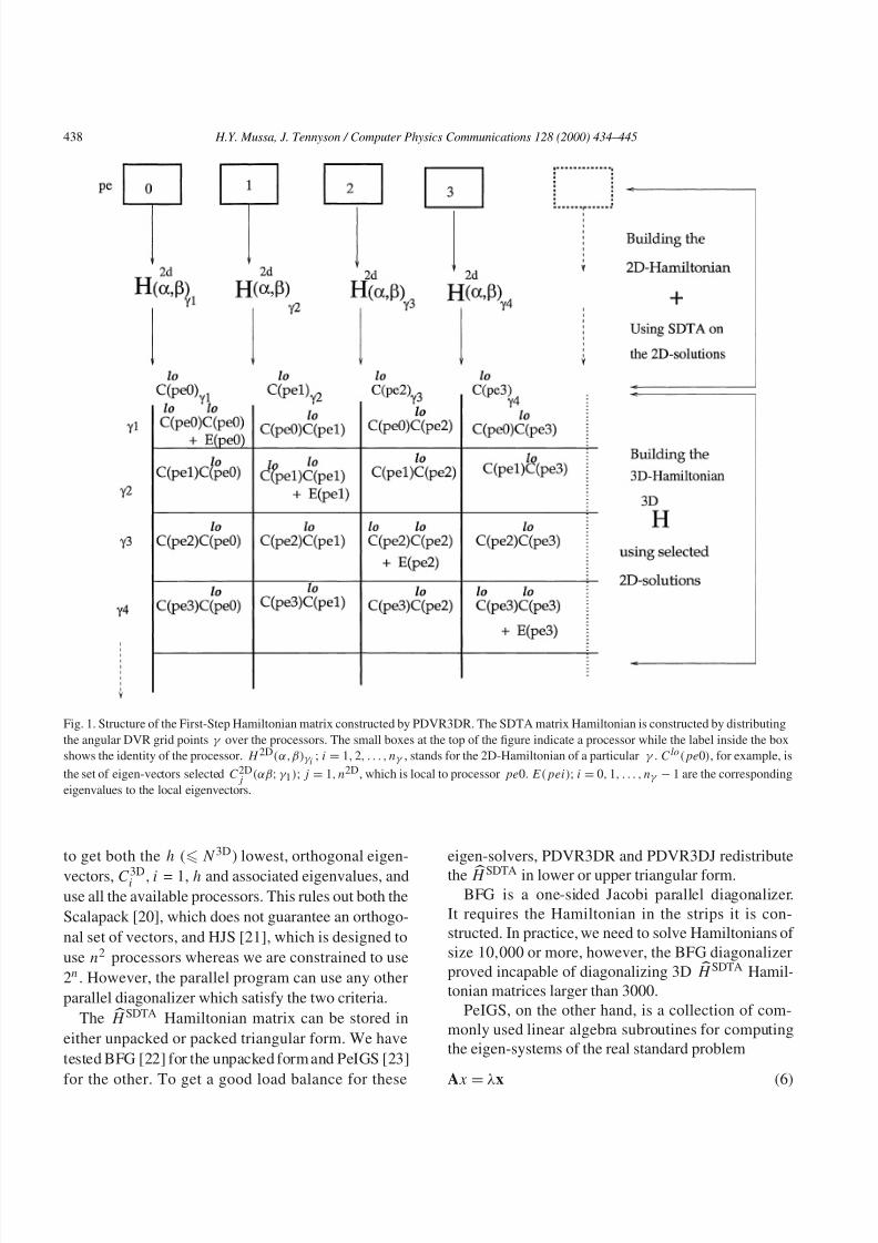
Fig. 1. Structure of the First-Step Hamiltonian matrix constructed by PDVR3DR. The SDTA matrix Hamiltonian is constructed by distributing

the angular DVR grid points γ over the processors. The small boxes at the top of the figure indicate a processor while the label inside the box

shows the identity of the processor. H 2D(α,β)γ i ; i = 1, 2, . . . , nγ , stands for the 2D-Hamiltonian of a particular γ . Clo(pe0), for example, is

the set of eigen-vectors selected C2Dj

(αβ; γ 1); j = 1, n2D, which is local to processor pe0. E(pei); i = 0, 1, . . . , nγ − 1 are the corresponding

eigenvalues to the local eigenvectors.

to get both the h ( N 3D) lowest, orthogonal eigen-

vectors, C3Di , i = 1, h and associated eigenvalues, and

use all the available processors. This rules out both the

Scalapack [20], which does not guarantee an orthogo-

nal set of vectors, and HJS [21], which is designed to

use n2 processors whereas we are constrained to use

2n. However, the parallel program can use any other

parallel diagonalizer which satisfy the two criteria.

The H SDTA Hamiltonian matrix can be stored in

either unpacked or packed triangular form. We have

tested BFG [22] for the unpacked form and PeIGS [23]

for the other. To get a good load balance for these

eigen-solvers, PDVR3DR and PDVR3DJ redistribute

the H SDTA in lower or upper triangular form.BFG is a one-sided Jacobi parallel diagonalizer.

It requires the Hamiltonian in the strips it is con-

structed. In practice, we need to solve Hamiltonians of

size 10,000 or more, however, the BFG diagonalizer

proved incapable of diagonalizing 3D H SDTA Hamil-

tonian matrices larger than 3000.

PeIGS, on the other hand, is a collection of com-

monly used linear algebra subroutines for computing

the eigen-systems of the real standard problem

Ax = λx (6)




and the general eigen-system

Ax = λBx, (7)

where A and B are dense and real symmetric matri-

ces with B positive definite and x is an eigenvector

corresponding to eigenvalue λ. PeIGS uses a flexible

column distribution with packed storage for real sym-

metric matrices which are similar to the H SDTA. A se-

rious drawback of PeIGS is its requirement for large

amount of memory as workspace.

As standard real symmetric diagonalizers limited

the size of calculations which could be attempted for

3D compact dense Hamiltonians, we also explored

the possibility of using an iterative parallel eigen-solver. Such an approach has been advocated by

a number of other workers [18,24–26], although,

unlike many of the studies, we require eigenvectors as

well as eigenvalues. To our knowledge there is only

one parallel iterative eigen-solver, PARPACK [27],

generally available.

PARPACK is a portable implementation of

ARPACK [28] for distributed memory parallel archi-

tectures. ARPACK is a package which implements the

Implicit Restarted Arnoldi Method used for solving

large sparse eigenvalue problems [27].Typically the blocking of the initial vector V is

commensurate with the parallel decomposition of the

matrix H SDTA. The user is free, however, to select an

appropriate blocking of V such that an optimal balance

between the parallel performance of PARPACK and

the user supplied matrix–vector product is achieved.

Interprocessor communication is inevitable, which

can create large overheads, to perform the matrix-

vector product as both the Hamiltonian matrix and the

vector are distributed over the processors. To avoid

any unnecessary interprocessor communications, we

perform our matrix–vector product

w = H SDTAV (8)

by using mpi_allreduce(V,x,n, mpi_real, mpi_sum,

comm, ierr ). Each processor then does the matrix–

vector multiplication on its local portions using the

sgemv BLAS [29].

In the matrix–vector description given above, the

H SDTA Hamiltonian is constructed beforehand. How-

ever, as suggested by WH [18], one can perform the

matrix–vector without explicitly constructing H SDTA.

Table 1

Comparison between PeIGS and PARPACK performance in the

solution of vibrational Hamiltonian matrix of dimension N = 3200

for the first 300 eigenvalues of different systems. The comparison

was conducted using 8 EPCC Cray-T3E processors

Molecule PeIGS/sec PARPACK/sec

H2O 245.3 104.7

HN+2

236.6 78.2

H+3

236.3 564.2

O3 236.0 177.0

In this approach the multiplication (in matrix nota-tion), see Eqs. (3)–(5), can be given by

y =

E2D + C(2D)γ LC(2D)γ

V . (9)

The advantage of WH’s scheme is that their method

requires less memory than ours, but as is clear from

Eqs. (8) and (9), our approach needs a smaller number

of operations per iteration. Therefore, as most of the

CPU time is spent on the diagonalization, our method

should perform better. As discussed in Section 5.3,

we have used other strategies to overcome memoryproblems when they arise.

In addition to the memory requirements and flexi-

bility, speed of the eigen-solver is another factor for

which one might choose the eigen-solver. When tested

on different systems, we found the relative perfor-

mance of PeIGS and PARPACK to be molecule de-

pendent, see Table 1.

In particular we found that for a given matrix size,

PeIGS timings are almost system independent. Con-

versely the iterative diagonalizer shows strong system

dependence, performing much worse for the stronglycoupled H+3 molecule, in which the spectra is dense

and the Hamiltonian eigenvalue distribution is low, but

very well for the others. Furthermore, it is known that

the speed of the PARPACK algorithm is dependent on

the H SDTA Hamiltonian eigenvalue distribution [18].

So this explains the convergence speed difference for

PARPACK in the table. Similar behaviour for itera-

tive diagonalizers on conventional computers was ob-

served by Bramley and Carrington [24]. It should be

noted that the comparisons are performed for a rela-

tively small final matrix and on only 8 processors.




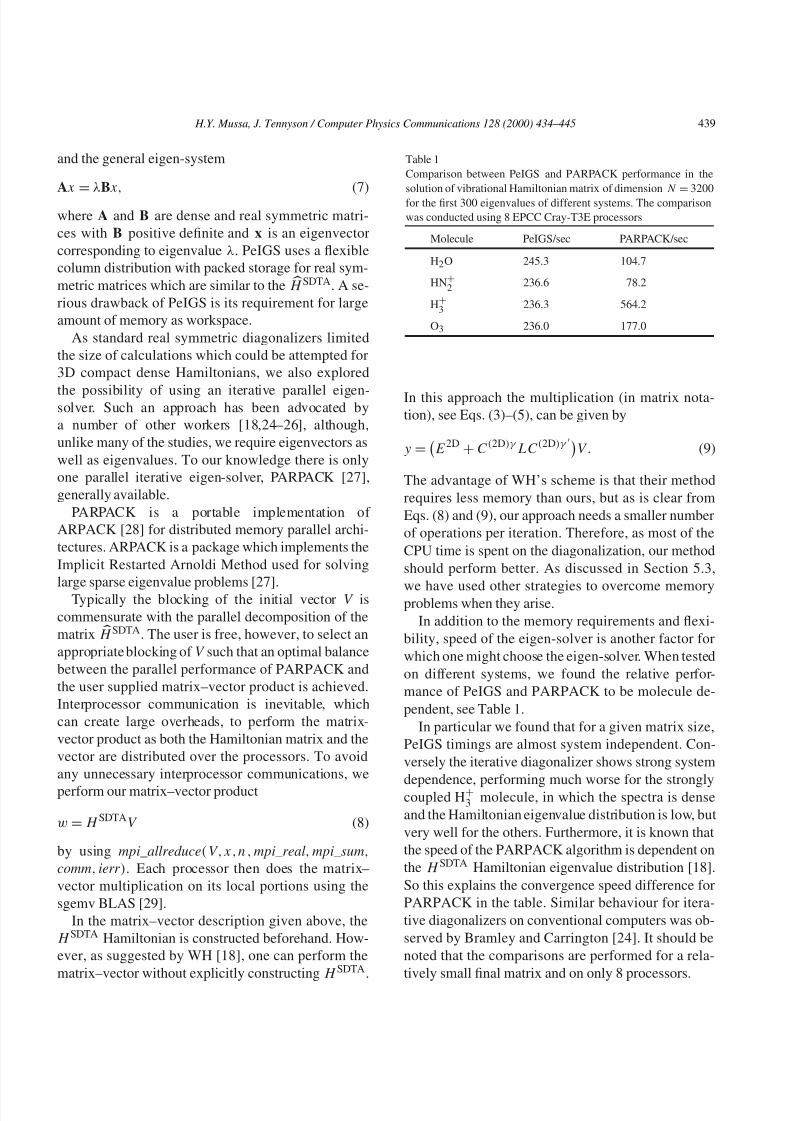
In PDVR3DR we therefore distributed the build-

ing of the off-diagonal blocks in k , Bk,k (h,h), over

the M processors by placing k

(nαnβ nγ ,h/M) and

k(nα nβ nγ , h/M) vectors on each processor. Each

processor thus builds rows of each block, Bk,k(h/M,

h). This is done using the vectors,k(nαnβ nγ ,h/M)

and k

(nα nβ nγ ,h/M), which are in the local

memory and non-local k(nα nβ nγ , h/M) vec-

tors. For example, for processor 0 to build its por-

tion of the block, Bk,k (h/M,h), it uses its local

k(nαnβ nγ ,h/M) and k

(nα nβ nγ , h/M) vectors

from other processors, see Fig. 2. This procedure is

repeated for each block formed.

However, it should be noted that the above scheme

requires two transformed vectors, k and keach

time. As it is necessary to minimize I/O on the

employed MPP machines and keeping all thes, J +

1 of them for each J , would require more real memory

than what is available, we employ an algorithm which

ensures that no more than three sets of vectors are

retained in memory at any one time. The following

steps show how the procedure works:

(1) For k = 0; create ψk=0 .

(2) For k = 1: create ψk=1

;form Bk=1,k=0, using Eq. (11) , k = k + 1.

Gather all the portions on processor 0 and then let

it write full block on a disk.

(3) For k = 2 to J : create ψk ;

form Bk,k , using Eq. (11), k = k + 2;

replace ψk+2 by ψk+1;

form Bk,k , using Eq. (11), k = k + 1;

Gather all the portions on processor 0 and then let

it write full block to disk.

This algorithm uses significantly less I/O than the one

presented in I.

5.2. PDVR3DJ

In PDVR3DJ the body-fixed z-axis is taken to be

parallel to one of the radial co-ordinates. This embed-

ding leads to a simpler Hamiltonian in which the Cori-

olis coupling only couples neighboring k blocks, i.e. k

with k ± 1 [7,30]. These off-diagonal elements have a

particularly simple form if the angular co-ordinates is

first transformed to associated Legendre polynomials,

|dj,k. The back transformed eigenvector is [7]

Qikαβj =

γ

T γ j ψik

αβγ . (12)

As for PDVR3DR, the construction of the fully cou-

pled Hamiltonian is reduced to constructing the terms

off-diagonal in k [7]. Here it is also necessary to par-

allelize the DVR to associated Legendre polynomial

transformation. As the vectors are distributed over the

processors, a copy of the transformation matrix, T γ

j ,

is duplicated on every processor. As a result the trans-formation is done without any need for inter-processor

communications. The off-diagonal block construction

step then consists of a series of transformations whichare performed in a similar fashion to PDVR3DR, but

as they are only three-dimensional, see Ref. [7], are

considerably less time consuming.

5.3. PROTLEV

The fully coupled rotation-vibration Hamiltonian

matrix is given by

Hk,k

= δk,k Ek + Bk,k

, (13)

where Ek is a vectorand Bk,k

is a matrix. PROTLEV3/ PROTLEV3B reads the eigenvalues and the off-diago-nal blocks from the disk. One processor does the read-

ing and then broadcast the data to the rest. Both Ek and

Bk,kmatrix elements are redistributed over the nodes,

such that there is an equal portion of the full Hamil-

tonian on each processor.

However, the resulting structure depends on the

eigen-solver used, see I for more details. As the size of

the Hamiltonian is given by h × (J + 1), and typically

h is between 1500 (H2O) and about 4000 (HN+2 ), for

low J ’s the PeIGs is more suitable.At this point it is worthwhile explaining why we

extended I by introducing the M/nη algorithm, seeSection 3. Consider our HN+

2 calculations [17,19]

as an example. As the final J > 0 Hamiltonian is

expressed in terms of the First-Step eigen-pairs, the

more first-step solutions used, the better the statesconverge. To converge all the 4900 or so even parity

rotational states for J = 1, it is necessary to use 3000

to 4000 ‘vibrational’ eigenvectors for each k.As explained in Section 4, PARPACK is preferred

over PeIGS for solving the ‘vibrational’ problems. In




Fig. 2. Construction of the off-diagonal block in k , Bk,k(h,h). stands for the transformed eigenvectors which are explained in the text. pei;

i = 0, 1, . . . , n − 1 are the processors.

PARPACK Upper Hessenberg matrix [27] U h(nv, nv)

is replicated on every processor. Where nv = 2 × h.

Therefore for h = 4000, the U h(nv, nv) requires more

memory per node than is available. Instead of trying to

deal with the PARPACK Upper Hessenberg problem,

as WH did [18], we modified our earlier scheme

of nη/M 1, so that we can employ the PeIGS

diagonalizer.

In the new algorithm, H SDTA is distributed over M

processors. Where M nη. In this scheme, a M/nη

number of processors build and solve the (H 2D)η for

each η grid, but each processor retains a different

portion of the lowest n2D 2D eigen-pairs. After this the

construction of the 3D-Hamiltonian is carried out in a

fashion similar to that of the nη/M 1 method, see

Section 3.1. The only notable difference is that the new

method requires more inter-processor communication.

This is due to the fact that for each η the chosen set of

eigen-pairs from the (

H 2D)η solution is spread over

M/nη processors. As N 3D = n2D × nη, see Eq. (2),

the bigger M is the smaller the H SDTA portion on each

processor becomes. Consequently PeIGS requires less

memory per node and big Hamiltonians, which could

not be solved with the nη/M 1 method, can be

diagonalized on a larger number of processors.

This trick enabled us to calculate all the rotational

states of HN+2 for J = 1; within a tenth of a wavenum-

ber or better [17,19]. This calculation showed that a

previous study on rotationally excited states of this

system gave results which were not converged [32].




6. Resonances

In principle, quasi-bound states can be defined usingdifferent properties of the wavefunction [33]. How-

ever, recent methods have employed optical potentials,

finite square integrable bases and diagonalization pro-cedures [26,34,35].

Using such a procedure to obtain resonance states,

it is necessary to solve

H = HSDTA − iU(η). (14)

U is the so-called optical potential which is introducedin the asymptotic region of the real potential V . η is the

dissociative co-ordinate and usually is the co-ordinate

treated last, see Section 3.As constructing and diagonalizing the complex

Hamiltonian in its above form could be both time

and computer memory consuming, we first solve theH SDTA and then use some of the eigen-pairs as basis

for constructing the H . For J = 0 in this basis, matrix

elements of the complex Hamiltonian can be written

as

ψnαβγ |

H |ψmαβγ = enδnm − iψn

αβγ |U |ψmαβγ . (15)

Within a DVR, the above equation can be simplified

further as

ψnαβγ |

H |ψmαβγ = enδnm − i

αβγ

ψnαβγ ψ

mαβγ U (ηγ ).

(16)

Where ψi is defined by Eq. (10).

Constructing the full Hamiltonian in parallel is quite

simple. It is similar to the H SDTA formation dis-cussed in Section 3. When n = m, the diagonal blocks

are formed using the locally available transformed

eigenvectors, whereas for n = m case, each proces-

sor should receive the required ψmαβγ from another

processor. In this procedure each processor builds aH (N/p,N) portion of the Hamiltonian; N being the

size of the Hamiltonian and p is the number of proces-

sors employed.

PARPACK is used for diagonalizing the complex

Hamiltonian matrix where the imaginary part of the

resulting eigenvalues yields an estimate for the width

of the resonance and the real part gives the energy.

However, to obtain well converged resonance states,it is necessary to vary the range and height of U,

and possibly the number of basis functions used.

As diagonalizing the H SDTA Hamiltonian again and

again, or writing on and reading from a disk in each

time is costly, we solve H SDTA

once and keep the ψ

sin core. Only the construction and diagonalization of H with different complex potential parameters and

different number of basis is repeatedly performed.Recently Skokov and Bowman [35] computed HOCl

resonance states for the potential energy surface (PES)

of Skokov et al. [36]. We have tested our resonance

algorithm for HOCl using the PES of Skokov et al.

For Cl–OH Jacobi coordinates, we used 35, 80 and 80

DVR grid points for r1(= rOH), r2 and θ , respectively.

r2, the dissociating coordinate, was treated last.

Building, diagonalizing and truncating the 2D-Ha-

miltonian takes 18.4 minutes. Constructing a final

compact 3D Hamiltonian of 6400 dimension, costs

less than 2.5 minutes. PARPACK is then employed

for solving the H SDTA to yield 1200 eigen-pairs, well

above the dissociation limit [35]. The diagonalization

wall time, on 80 T3E-1200 processors, is 21 minutes.

Performing the the eigen-vectors transformation, see

Eq. (12), takes about 2 minutes.

For particular optical potential height and range,

all the 1200 transformed eigenvectors were used for

forming the complex Hamiltonian,

H (1200, 1200).

Only 3 minutes of real time was required to constructand diagonalize the Hamiltonian on the 80 processors.

It should be noted that only the eigenvalues were

calculated.

These results are only preliminary. We are currently

working on their optimization. Comparisons with the

HOCl results of Skokov and Bowman give excellent

agreement for resonance positions and widths whichagree within the accuracy of the method.

7. Program performance

The speed up of a program on M processors is given

by,

S M =T 1

T M

, (17)

where T M is the time it takes the program to run on

M processors. The speed up directly measures the ef-

fects of synchronization and communication delays on

the performance of a parallel algorithm. Ideally S M

should grow linearly with M . In practice, this is very




Table 2

PDVR3DJ performance on the Manchester University Cray T3E-

1200E in seconds for a triatomic molecule ‘vibrational’ calcula-

tions with J = 1 and a compact final Hamilt onian of dimension

N = 5120 for HN+2

. Note that only 512 eigenvectors were trans-

formed (see the text). np = number of processors. hcet = time for

Hamiltonain construction and the transformation of selected eigen-

vectors. bb = time for the k off-diagonal bloks formation. Finally

diag stands for the “vibrational” Hamiltonian diagonalization time.

Note that the time is in seconds

np hcet bb diag

16 1330.14 2180.25 1657.06

32 626.24 1113.88 885.99

64 300.67 566.20 498.02

128 147.88 285.38 311.92

unlikely because the time spent on each communica-

tion increases with the number of processors and thus

the scalability deteriorates when a large number of

processors is employed.

Here only the scalability for the PDVR3DJ and

PROTLEV3 will be discussed. We have tested the

performance of both PDVR3DJ and PROTLEV3 using

the Cray T3E-1200E at Manchester University.

Table 2 illustrates the scalability of the ‘vibra-tion’program PDVR3DJ using PeIGS for solving the

Hamiltonian. The Hamiltonian construction and the

transformation of the chosen eigenvectors procedure

shows near-perfect scalability, because the paralleliza-

tion strategy chosen minimizes data transfer, and us-

age of BLAS routines, which are optimized for the

MPP machines, maximizes the performance of the

floating point operations. The in-core diagonalizer,

PeIGS, requires considerable interprocessor commu-

nication so some degradation with increasing number

of processors is to be expected, see I. This problem ismagnified when eigenvectors are also required. This

is an intrinsic problem of parallel direct diagonalizers

where an implicit Gram-Schmidt step must be imple-

mented to conserve orthogonality between eigenvec-

tors extracted on different processors, see [37].

It should be noted that only 512 ‘vibrational’

eigenvectors, 10% of the total eigenvectors, were

transformed (see Section 5).

Table 3 shows the equivalent behaviour for

PROTLEV3, only in-core diagonalization, using PeIGS

is considered as it is rapid and gives all the eigen-pairs.

Table 3

PROTLEV3 performance on the Manchester University Cray T3E-

1200E in seconds for a triatomic molecule with J = 1 and a final

Hamiltonian of dimension N = 1024 for HN+2

. See the text for

more details. np = number of processors and fc = fully foupled

Hamiltonian Solution. The time is in seconds

np fc

2 84.05

4 46.12

8 27.55

16 16.83

32 12.92

In this case matrix construction requires I/O. Since

the I/O gates are not dedicated to us, this may intro-

duce some arbitrariness to the performance. However,

the actual Hamiltonian construction time is small.

Therefore the diagonalization is the main feature in

PROTLEV3. So the above argument applies and in-

deed confirmed by the figure.

8. Conclusions

We have developed parallel programs for treating

the vibration-rotation motion of the three-atom system

using either Jacobi or Radau co-ordinates. These pro-

grams are based on the published DVR3D program [7]

which is designed for computers with traditional archi-

tectures. Significant algorithm changes were required,

in particular to reduce I/O interfaces in the original

programs. The parallel suite shows good scalabilityand can be used for big and challenging calculations.

Generally tests of presently available parallel eigen-

solvers favor the iterative eigen-solvers for their low

workspace requirements.

Employing the parallel code we have studied the

rotation-vibration of a number of key triatomic sys-

tem, such as H2O, O3, HN+2 , H+

3 , and HCP. We have

extended the parallel program to look at vibrational

resonances which we have studied for HOCl. We are

currently extending our method to the resonances in

rotationally excited molecules.




Acknowledgement

This work was performed as part of the ChemReactHigh Performance Computing Initiative (HPCI) Con-

sortium. We thank Robert Allan and the members of

HPCI centres at Daresbury Laboratory, ManchesterUniversity and Edinburgh University for their help.

We also thank Dr. Serge Skokov for supplying his

HOCl potential energy surface.

References

[1] J. Tennyson, B.T. Sutcliffe, J. Chem. Phys. 77 (1982) 4061.

[2] S. Carter, N.C. Handy, Mol. Phys. 52 (1984) 1367.

[3] J.S. Lee, D. Secrest, J. Chem. Phys. 92 (1988) 182.

[4] D. Estes, D. Secrest, Mol. Phys. 59 (1986) 569.

[5] G.J. Harris, S. Viti, H.Y. Mussa, J. Tennyson, J. Chem. Phys.

109 (1998) 7197.

[6] H.Y. Mussa, J. Tennyson, C.J. Noble, R.J. Allan, Comput.

Phys. Commun. 108 (1998) 29.

[7] J. Tennyson, J.R. Henderson, N.G. Fulton, Comput. Phys.

Commun. 86 (1995) 175.

[8] H.Y. Mussa, J. Tennyson, J. Chem. Phys. 109 (1998) 10 885.

[9] Z. Bacic, J.C. Light, Annu. Rev. Phys. Chem. 40 (1989) 469.

[10] B.T. Sutcliffe, J. Tennyson, Int. Quantum Chem. 29 (1991)

183.

[11] Message Passing Interface; the MPI Standard is available from

netlib2.cs.utk.edu by anonymous ftp.[12] M.J. Bramley, T. Carrington, Jr., J. Chem. Phys. 101 (1994)

8494.

[13] J.R. Henderson, C.R. Le Sueur, S.G. Pavett, J. Tennyson,

Comput. Phys. Commun. 74 (1993) 193.

[14] N.G. Fulton, PhD Thesis, London University (1995).

[15] NAG Fortran Library Manual, Mark 17, Vol. 4 (1996).

[16] LAPACK Users’ Guideis available in html form from WWW

URL http://www.netlib.org/lapack/lug/lapack_lug.html.

[17] H.Y. Mussa, PhD Thesis, London University (1998).

[18] X.T. Wu, E.F. Hayes, J. Chem. Phys. 107 (1997) 2705.

[19] H.Y. Mussa, S. Schmatz, M. Mladenovic, J. Tennyson,

J. Chem. Phys. (to be submitted).

[20] Scalapack Users’ Guide is available in html form from WWW

URL http://www.netlib.or. org/scalapack/.

[21] B.A. Henderson, E. Jessup, C. Smith, A parallel eigensolver for

a parallel eigensolver for dense symmetric matrices, available

via anonymous ftp from ftp.cs.sandia.gov/pub/papers/bahendr/

eigen.ps.Z.

[22] I.J. Bush, Block factored one-sided Jacobi routine, following:

R.J. Littlefield, K.J. Maschhoff, Theor. Chim. Acta 84 (1993)

457.

[23] G. Fann, D. Elwood, R.J. Littlefield, PeIGS Parallel Eigen-

solver System, User Manual available via anonymous ftp from

pnl.gov.

[24] M.J. Bramley, T. Carrington Jr, J. Chem. Phys. 99 (1993) 8519.

[25] M.J. Bramley, J.W. Tromp, T. Carrington Jr, G.C. Corey,

J. Chem. Phys. 100 (1994) 6175.

[26] V.A. Mandelshtam, H.S. Taylor, J. Chem. Soc. Faraday Trans.

93 (1997) 847.[27] R. Lehoucq, K. Maschhoff, D. Sorensen, C. Yang, PARPACK,

available from ftp://ftp.caam.rice.edu/pub/allowbreak people/

kristyn.

[28] R.B. Lehoucq, D.C. Sorensen, P.A. Vu, C. Yang, ARPACK:

Fortran subroutines for solving large scale eigenvalue prob-

lems. The ARPACK package is available from http://www.

caam.rice.edu/software/ARPACK/index.html.

[29] BLAS Users’ Guide is available in html form from WWW

URL http://www.netlib.org/blas/lug/blas.html.

[30] J. Tennyson, B.T. Sutcliffe, Int. Quantum Chem. 42 (1992)

941.

[31] E.M. Goldberg, S.K. Gray, Comput. Phys. Commun. 98

(1996) 1.[32] S. Schmatz, M. Mladenovic, Ber. Bunsenges. Phys. Chem. 101

(1997) 372.

[33] B.R. Junker, Advan. At. Mol. Phys. 18 (1982) 287.

[34] G. Jolicard, E.J. Austin, Chem. Phys. 103 (1986) 295.

[35] S. Skokov, J.M. Bowman, J. Chem. Phys. 110 (1999) 9789.

[36] S. Skokov, J. Qi, J.M. Bowman, K.A. Peterson, J. Chem. Phys.

109 (1998) 2662.

[37] G. Fann, R.J. Littlefield, Parallel inverse iteration with re-

orthoganalisation, in: Proc. 6th SIAM Conf. Parallel Process-

ing for Scienticif Computing (SIAM, Philadelphia, PA, 1993)

p. 409.

Hamse Y. Mussa and Jonathan Tennyson- Bound and quasi-bound rotation-vibrational states using...

Documents

Transcript of Hamse Y. Mussa and Jonathan Tennyson- Bound and quasi-bound rotation-vibrational states using...