HadSST.4.0.1.0 Product User Guide

J.J. Kennedy, N.A. Rayner, C.P. Atkinson, R.E. Killick

September 24, 2021

Citation: Kennedy, J.J., Rayner, N.A., Atkinson, C.P., and Killick, R.E. (2019). An ensemble data set of sea surfacetemperature change from 1850: the Met Office Hadley Centre HadSST.4.0.0.0 data set. Journal of Geophysical Research:Atmospheres, 124. https://doi.org/10.1029/2018JD029867

1

EMERGENCY ONE PAGE QUICK START GUIDE FOR HadSST.4.0.1.0HadSST.4.0.1.0 is the Met Office Hadley Centre Sea-surface temperature anomaly data set. Anomalies are expressed relativeto the 1961-1990 average. The data have been adjusted to minimize the effect of systematic errors associated with instrumen-tation changes and are representative of SST measured at a depth of 20cm. The data set is presented on an equi-rectangular 5°latitude by 5° longitude monthly grid from January 1850 to present.

Uncertainty in the data is presented using a combined approach. Uncertainty in the bias adjustments is presented as anensemble of interchangeable realisations. Uncertainty arising from local measurement errors and local sampling errors arepresented as gridded fields. Uncertainties associated with correlated measurement errors are presented as error-covariancematrices. These can be combined to give uncertainty estimates for derived quantities such as the global mean temperature.

HadSST.4.0.1.0 is based on ICOADS release 3.0.0 (1850-2014, [6]) and ICOADS release 3.0.1 (2015-present). In additionit uses drifting buoy observations “Generated using E.U. Copernicus Marine Service Information” from CMEMS.

What products are available?The following products are available under the Open Government License v3. The basic time series products are:

• Global average SST anomaly with uncertainties, link

• Regional average SST anomalies with uncertainties, link

The basic gridded products are:

• Grid of median SST anomalies calculated from the ensemble, monthly 1850-present, link

• Grids of bias-adjusted SST anomalies for the 200 ensemble members, monthly 1850-present, link

• Grid of estimated uncertainties arising from all sources, monthly 1850-present, link

There are other products including individual components of uncertainty, error covariances (for propagating uncertainty prop-erly) and counts of numbers of observations.

How do I obtain the data?Data are available from http://www.metoffice.gov.uk/hadobs/hadsst4/ and specific links are given above. Data and productsare made available under the Open Government License v3.

How do I read the HadSST.4.0.1.0 data?The time series data are stored in csv (Comma Separated Value) files which can be read by a wide variety of tools includingExcel. The gridded data are stored in NetCDF format files. NetCDF files are a platform-independent, self-describing binaryformat and there are a number of common tools (Section 3.2) that can be used to access the data. Some basic python code isprovided in Section 4 to show worked examples of reading the data and performing some simple calculations and processing.

What tools are available for these products?Some basic python code is provided in Section 4 to show worked examples of reading the data and performing some simplecalculations and processing.

How to acknowledge and cite the data setWe recommend that users of the data specify which version of the data set they used, when the data were downloaded, providea link to the website and a link to the license. For example:

HadSST.4.0.1.0 data were obtained from http://www.metoffice.gov.uk/hadobs/hadsst4/data on [date downloaded]and are ©British Crown Copyright, Met Office [year of download] provided under an Open Government Licensev3 http://www.nationalarchives.gov.uk/doc/open-government-licence/version/3/.

2

In addition, users of HadSST.4.0.1.0 are kindly requested to cite the specific journal article:

Kennedy, J.J., Rayner, N.A., Atkinson, C.P., and Killick, R.E. (2019). An ensemble data set of sea surfacetemperature change from 1850: the Met Office Hadley Centre HadSST.4.0.0.0 data set. Journal of GeophysicalResearch: Atmospheres, 124. https://doi.org/10.1029/2018JD029867.

Further information and contactFor further help please read the rest of the document. The paper describing the data set is the best place to find the technicaldetails. Updated diagnostics are available from http://www.metoffice.gov.uk/hadobs/hadsst4/. For further enquiries contactjohn.kennedy@metoffice.gov.uk. Data set updates will be tweeted from @metofficeHadOBS

3

Contents1 Getting started with HadSST.4.0.1.0 6

1.1 How do I get the data? . . . . . . . . . . . . . . . . . . . . . . . . . . . . . . . . . . . . . . . . . . . . . . 61.1.1 Time series data . . . . . . . . . . . . . . . . . . . . . . . . . . . . . . . . . . . . . . . . . . . . . 61.1.2 Gridded data . . . . . . . . . . . . . . . . . . . . . . . . . . . . . . . . . . . . . . . . . . . . . . . 6

1.2 How do I use the data? . . . . . . . . . . . . . . . . . . . . . . . . . . . . . . . . . . . . . . . . . . . . . . 71.2.1 Dos and Donts of using the data . . . . . . . . . . . . . . . . . . . . . . . . . . . . . . . . . . . . . 7

1.3 How do I use the uncertainty estimates? . . . . . . . . . . . . . . . . . . . . . . . . . . . . . . . . . . . . . 71.3.1 Propagating uncertainty associated with uncorrelated errors . . . . . . . . . . . . . . . . . . . . . . 71.3.2 Propagating uncertainty associated with simply-correlated errors . . . . . . . . . . . . . . . . . . . . 81.3.3 Propagating uncertainty using the ensemble . . . . . . . . . . . . . . . . . . . . . . . . . . . . . . . 91.3.4 Combing the propagated uncertainty components . . . . . . . . . . . . . . . . . . . . . . . . . . . . 91.3.5 Caveats . . . . . . . . . . . . . . . . . . . . . . . . . . . . . . . . . . . . . . . . . . . . . . . . . . 9

1.4 Basic data statistics . . . . . . . . . . . . . . . . . . . . . . . . . . . . . . . . . . . . . . . . . . . . . . . . 101.5 Contact us . . . . . . . . . . . . . . . . . . . . . . . . . . . . . . . . . . . . . . . . . . . . . . . . . . . . 111.6 FAQ . . . . . . . . . . . . . . . . . . . . . . . . . . . . . . . . . . . . . . . . . . . . . . . . . . . . . . . . 11

1.6.1 Is HadSST.4.0.1.0 the data set for me? . . . . . . . . . . . . . . . . . . . . . . . . . . . . . . . . . . 111.6.2 What anomaly period have you used? . . . . . . . . . . . . . . . . . . . . . . . . . . . . . . . . . . 111.6.3 Why do you use anomalies and not actual SSTs? . . . . . . . . . . . . . . . . . . . . . . . . . . . . 111.6.4 Where do the observations come from? . . . . . . . . . . . . . . . . . . . . . . . . . . . . . . . . . 121.6.5 How does HadSST.4.0.1.0 differ from HadSST.3.0.0.0 and HadISST? . . . . . . . . . . . . . . . . . 121.6.6 Why are there 200 different data sets? . . . . . . . . . . . . . . . . . . . . . . . . . . . . . . . . . . 121.6.7 What restrictions are there on the data? What is the data license? . . . . . . . . . . . . . . . . . . . . 121.6.8 How to acknowledge and cite the data? . . . . . . . . . . . . . . . . . . . . . . . . . . . . . . . . . 121.6.9 There are gaps in the data, what can I do? . . . . . . . . . . . . . . . . . . . . . . . . . . . . . . . . 131.6.10 What do the different parts of the version number mean in HadSST.4.0.1.0? . . . . . . . . . . . . . . 131.6.11 When should I use the total uncertainty and when should I use the uncertainty components? . . . . . 141.6.12 Why do the anomalies not average to zero in the climatology period? . . . . . . . . . . . . . . . . . 14

2 Using the time series files 142.1 File names . . . . . . . . . . . . . . . . . . . . . . . . . . . . . . . . . . . . . . . . . . . . . . . . . . . . . 142.2 Tools that can be used . . . . . . . . . . . . . . . . . . . . . . . . . . . . . . . . . . . . . . . . . . . . . . 142.3 Contents of the time series files . . . . . . . . . . . . . . . . . . . . . . . . . . . . . . . . . . . . . . . . . . 15

3 Using the gridded data files 153.1 File names . . . . . . . . . . . . . . . . . . . . . . . . . . . . . . . . . . . . . . . . . . . . . . . . . . . . 153.2 Tools that can be used to work with data files . . . . . . . . . . . . . . . . . . . . . . . . . . . . . . . . . . 163.3 Contents of data files . . . . . . . . . . . . . . . . . . . . . . . . . . . . . . . . . . . . . . . . . . . . . . . 17

3.3.1 SST anomalies: HadSST.4.0.1.0_median.nc . . . . . . . . . . . . . . . . . . . . . . . . . . . . . . . 173.3.2 SST anomalies: HadSST.4.0.1.0_unadjusted.nc . . . . . . . . . . . . . . . . . . . . . . . . . . . . . 183.3.3 SST anomalies: HadSST.4.0.1.0_ensemble_member_EEEE.nc . . . . . . . . . . . . . . . . . . . . . 183.3.4 SST actuals: HadSST.4.0.1.0_actuals_median.nc . . . . . . . . . . . . . . . . . . . . . . . . . . . . 183.3.5 SST actuals: HadSST.4.0.1.0_actuals_ensemble_member_EEEE.nc . . . . . . . . . . . . . . . . . . 183.3.6 SST anomalies: HadSST.4.0.1.0_number_of_observations.nc . . . . . . . . . . . . . . . . . . . . . 193.3.7 SST anomalies: HadSST.4.0.1.0_number_of_superobservations.nc . . . . . . . . . . . . . . . . . . . 193.3.8 SST anomalies: HadSST.4.0.1.0_total_uncertainty.nc . . . . . . . . . . . . . . . . . . . . . . . . . . 193.3.9 SST anomalies: HadSST.4.0.1.0_measurement_and_sampling_uncertainty.nc . . . . . . . . . . . . . 203.3.10 SST anomalies: HadSST.4.0.1.0_uncorrelated_measurement_uncertainty.nc . . . . . . . . . . . . . . 203.3.11 SST anomalies: HadSST.4.0.1.0_correlated_measurement_uncertainty.nc . . . . . . . . . . . . . . . 203.3.12 SST anomalies: HadSST.4.0.1.0_sampling_uncertainty.nc . . . . . . . . . . . . . . . . . . . . . . . 213.3.13 SST anomalies: HadSST.4.0.1.0_fractional_contribution_bucket.nc . . . . . . . . . . . . . . . . . . 213.3.14 SST anomalies: HadSST.4.0.1.0_fractional_contribution_eri.nc . . . . . . . . . . . . . . . . . . . . 213.3.15 SST anomalies: HadSST.4.0.1.0_fractional_contribution_hull.nc . . . . . . . . . . . . . . . . . . . . 223.3.16 SST anomalies: HadSST.4.0.1.0_fractional_contribution_unknown.nc . . . . . . . . . . . . . . . . . 22

4

3.3.17 SST anomalies: HadSST.4.0.1.0_fractional_contribution_drifter.nc . . . . . . . . . . . . . . . . . . 223.3.18 SST anomalies: HadSST.4.0.1.0_fractional_contribution_moored.nc . . . . . . . . . . . . . . . . . . 233.3.19 Error covariances: HadSST.4.0.1.0_error_covariance_YYYYMM.nc . . . . . . . . . . . . . . . . . 23

4 Worked examples 244.1 Calculate global mean SST time series . . . . . . . . . . . . . . . . . . . . . . . . . . . . . . . . . . . . . . 244.2 Calculate monthly area average and uncertainty . . . . . . . . . . . . . . . . . . . . . . . . . . . . . . . . . 24

5 Version history 255.1 HadSST.4.0.1.0 . . . . . . . . . . . . . . . . . . . . . . . . . . . . . . . . . . . . . . . . . . . . . . . . . . 255.2 HadSST.4.0.0.0 . . . . . . . . . . . . . . . . . . . . . . . . . . . . . . . . . . . . . . . . . . . . . . . . . . 265.3 HadSST.3.1.1.0 . . . . . . . . . . . . . . . . . . . . . . . . . . . . . . . . . . . . . . . . . . . . . . . . . . 275.4 HadSST.3.1.0.0 . . . . . . . . . . . . . . . . . . . . . . . . . . . . . . . . . . . . . . . . . . . . . . . . . . 275.5 HadSST.3.0.0.0 . . . . . . . . . . . . . . . . . . . . . . . . . . . . . . . . . . . . . . . . . . . . . . . . . . 275.6 HadSST2 . . . . . . . . . . . . . . . . . . . . . . . . . . . . . . . . . . . . . . . . . . . . . . . . . . . . . 275.7 HadSST . . . . . . . . . . . . . . . . . . . . . . . . . . . . . . . . . . . . . . . . . . . . . . . . . . . . . . 27

6 Dataset Characteristics 276.1 Intercomparisons with other SST datasets . . . . . . . . . . . . . . . . . . . . . . . . . . . . . . . . . . . . 276.2 Comparison to other long records . . . . . . . . . . . . . . . . . . . . . . . . . . . . . . . . . . . . . . . . . 306.3 Instrumentally homogeneous series . . . . . . . . . . . . . . . . . . . . . . . . . . . . . . . . . . . . . . . . 30

6.3.1 Argo . . . . . . . . . . . . . . . . . . . . . . . . . . . . . . . . . . . . . . . . . . . . . . . . . . . 306.3.2 ARC ATSR Reprocessing for Climate . . . . . . . . . . . . . . . . . . . . . . . . . . . . . . . . . . 306.3.3 Buoys . . . . . . . . . . . . . . . . . . . . . . . . . . . . . . . . . . . . . . . . . . . . . . . . . . . 33

6.4 Known issues arising in the literature . . . . . . . . . . . . . . . . . . . . . . . . . . . . . . . . . . . . . . . 336.5 Processing notes . . . . . . . . . . . . . . . . . . . . . . . . . . . . . . . . . . . . . . . . . . . . . . . . . . 33

6.5.1 Coverage uncertainty . . . . . . . . . . . . . . . . . . . . . . . . . . . . . . . . . . . . . . . . . . . 33

References 34

5

1 Getting started with HadSST.4.0.1.0This section describes some basic information about the HadSST.4.0.1.0 data set. HadSST.4.0.1.0 is a data set of sea-surfacetemperature anomalies. The data have been adjusted to minimize the effect of instrumentation changes. The data are pre-sented on a regular 5◦latitude by 5◦ longitude grid for each month from January 1850. Uncertainty estimates associated withmeasurement and sampling limitations are also provided. Uncertainty in the bias adjustments are represented by the useof an ensemble; there are 200 versions of the data set making different assumptions about the biases. The data set is notglobally-complete and there is little processing to smooth the fields beyond averaging the data onto a regular grid.

1.1 How do I get the data?Data are available from http://www.metoffice.gov.uk/hadobs/hadsst4/data where checksums for the files can also be found.The data and products are available under the Open Government License v3. There are time series files in csv format andgridded fields of SST anomalies, uncertainty information and numbers of observations in NetCDF format.

1.1.1 Time series data

The time series data are in csv (Comma Separated Value) format. There are monthly and annual series:

• Global annual mean SST anomaly series: HadSST.4.0.1.0_annual_GLOBE.csv

• Global monthly mean SST anomaly series: HadSST.4.0.1.0_monthly_GLOBE.csv

• Northern hemisphere annual mean SST anomaly series: HadSST.4.0.1.0_annual_NHEM.csv

• Northern hemisphere monthly mean SST anomaly series: HadSST.4.0.1.0_monthly_NHEM.csv

• Southern hemisphere annual mean SST anomaly series: HadSST.4.0.1.0_annual_SHEM.csv

• Southern hemisphere monthly mean SST anomaly series: HadSST.4.0.1.0_monthly_SHEM.csv

1.1.2 Gridded data

The gridded data are in NetCDF format. There are a number of different files. The most commonly used files are:

• Grid of median SST anomalies calculated from the ensemble, monthly 1850-present, link

• Grids of bias-adjusted SST anomalies for the 200 ensemble members, monthly 1850-present, link

• Grid of estimated uncertainties arising from all sources, monthly 1850-present, link

Additional information is provided in the following files:

• Grid of measurement and sampling uncertainty, monthly 1850-present, link

• Grid of uncorrelated measurement uncertainty, monthly 1850-present,link

• Grid of correlated measurement uncertainty, monthly 1850-present,link

• Grid of sampling uncertainty, monthly 1850-present,link

• Grid of number of observations, monthly 1850-present,link

• Grid of number of super obserations, monthly 1850-present,link

• Error covariance matrices, monthly 1850-present,link

There are also files containing “actual” SSTs (as opposed to anomalies):

• Grids of median actual SST calculated from the ensemble, monthly 1850-present, link

• Grids of bias-adjusted actual SST for the 200 ensemble members, monthly 1850-present, link

6

1.2 How do I use the data?The data are in NetCDF format, which is a standard data format for climate data. Furthermore, the data files are CF compliantwhich means that the metadata in the files is in a standardised format. The structure of the data files is described in more detailin Section 3. Some example code for reading and processing the data is found in Section 4. The gridded data are stored in a3-dimensional array, with dimensions of time x longitude x latitude. There are 72 longitude points and 36 latitude points. The72 longitude points represent 5◦ grid cells with centres running from −177.5◦E to +177.5◦E. The 36 latitude points representgrid cells with centres running from −87.5◦N to +87.5◦N.

1.2.1 Dos and Donts of using the data

Do - be aware that there are gaps in the data and that there can be considerable “noise” in less-well-observed grid cells.Auxiliary products like the uncertainty estimates and the number of observations files can provide useful additionalinformation for identifying grid cells in which the uncertainty is likely to be large.

Do - use the uncertainty information (see next section). It will help you to understand the relative reliability of the data as thischanges markedly over time and in different places.

Don’t - compare HadSST.4.0.1.0 to globally complete SST analyses without taking into account the gaps in the data. Datacoverage can affect the comparability of two data sets.

Do - use the files of actual SSTs if you need actual SSTs. However, be careful when calculating area averages from the actualSSTs because the changing geographical coverage has a much greater effect when averaging actual SSTs than it doeswhen averaging SST anomalies.

Do - read the Open Government License v3.

Do - send us feedback when you use the data to john.kennedy@metoffice.gov.uk.

1.3 How do I use the uncertainty estimates?The uncertainty analysis is one of the more complex parts of using HadSST.4.0.1.0. The following information provides abasic guide to using the uncertainty information provided with the data set. Every effort has been made to make this processas painless as possible, but it can still be somewhat painful. It is worth it though.

The uncertainty has been broken down into three separate components, each of which represents errors with differentdegrees of correlation. The separate components need to be propagated individually through any calculation and combined atthe end to get an estimate of the overall uncertainty. The three components are:

1. Uncorrelated measurement and sampling error component, provided as gridded fields on the same 5x5x1-month gridas the SST anomalies. They represent uncertainties arising from uncorrelated measurement errors and local undersampling. In most cases the uncertainty for this kind of error can be propagated analytically.

2. Simply-correlated measurement error component, provided as an error-covariance matrix. The error-covariance matri-ces represent errors such as individual ship biases that can be represented by an error-covariance matrix. In many casesthe uncertainty for this kind of error can be propagated analytically.

3. The spread of the 200 members of the ensemble represents the uncertainty in the bias adjustments. The ensemblerepresents errors with complex correlation structures. In most cases, the uncertainty associated with this kind of errorcannot be propagated analytically, which is why we use an ensemble.

Each of these components should be propagated separately through any calculation and then combined at the end

1.3.1 Propagating uncertainty associated with uncorrelated errors

Propagation of uncertainties associated with uncorrelated errors are relatively easy to deal with using the standard propagationof errors formula. If the SST anomalies are being processed through a function f (x1,x2,...,xn)where x1,x2...xnare the griddedSST anomalies with uncertainties σ1,σ2...σnthen the uncertainty in f , σ f is given by

σ2f =

n

∑i=1

(∂ f∂xi

)2

σ2i (1)

7

So, for a weighted average, such as the global average where the area of each grid cell is withen

f =n

∑i=1

wixi (2)

and the uncertainty in the global average arising from uncorrelated errors is given by:

σ2f =

n

∑i=1

w2i σ

2i (3)

If there are multiple steps in the processing then the uncertainty can often be propagated through each step separately. Forexample, if we want to calculate an annual global average we can take the uncertainties in the twelve monthly global averages,call them σmonth, and combine them like so:

σ2annual =

Dec

∑month=Jan

(1

12

)2

σ2month (4)

Care must be taken though because if data values are used more than once in the calculation, then errors in different partsof the calculation will become correlated and these simple formulae won’t work.

1.3.2 Propagating uncertainty associated with simply-correlated errors

The propagation of uncertainty associated with simply-correlated errors is slightly more complex than for uncorrelated errors.For an error-covariance matrix E the uncertainty in f would be

σ2f =

n

∑i=1

n

∑j=1

(∂ f∂xi

∂ f∂x j

Ei j

)(5)

so for our example above of the global average, the uncertainty in f would become

σ2f =

n

∑i=1

n

∑j=1

wiw jEi j (6)

A more compact way of writing this (and calculating it) is to use vector and matrix notation. If we have a vector of weightsw then the uncertainty in f becomes simply:

σ2f = wEwT (7)

Unlike the case of uncorrelated errors, it is usually not so simple to propagate simply-correlated errors through multipleprocessing steps. There are, however, a number of approaches.

First, one can combine the separate calculation steps. For example, if you want to calculate the uncertainty in the differencebetween the northern hemisphere average and the southern hemisphere average then one can combine the two calculationsinto one where

f =n

∑i=1

wixi −n

∑i=1

vixi =n

∑i=1

(wi − vi)xi (8)

where wiis the weight a grid box gets in the northern hemisphere average (and zero for any grid box in the southernhemisphere) and vi is the weight given to grid box i in the southern hemisphere average (again, zero for any grid box in thenorthern hemisphere). The uncertainty in f is then

σ2f =

n

∑i=1

n

∑j=1

(wi − vi)(w j − v j)Ei j (9)

or, using vector and matrix notation,σ

2f = (w−v)E (w−v)T (10)

An alternative approach is to draw samples from a multi-variate Gaussian distribution with mean zero and covariance setequal to the error-covariance matrix. These samples can then be added to the SST anomalies to generate an ensemble and thetechniques used in the next section to deal with ensembles can be employed to propagate the uncertainty. Sampling from amulti-variate Gaussian distribution is relatively easy to do in two steps:

8

1. Calculate the Cholesky decomposition A of HEHT , where E is the error covariance matrix and H is a matrix, consistingof 1s and 0s that selects out the n non-missing data points.

2. Draw n independent standard normal values and put them into a vector z

3. Calculate x = Az. The vector x will now contain a sample of n correlated errors which can be added to the n SSTanomalies.

4. Repeat steps 2 and 3 to build up an ensemble.

This method can be combined with samples drawn from the uncorrelated error component and the ensemble to propagate allerror types simultaneously.

Temporal averaging is tricky because, as yet, there are no error covariances which describe the temporal relationship ofsimply-correlated errors. In the paper, it is generally assumed that at a global level, the simply-correlated errors are perfectlycorrelated from one time step to the next within a year, but uncorrelated between years. This approximation is unlikely to berealistic for individual grid cells as the chances of a ship or buoy revisiting the same grid cell vary geographically.

1.3.3 Propagating uncertainty using the ensemble

In many ways this is the simplest of the three types of error to deal with. If we have n ensemble members then we can calculatethe uncertainty on f by calculating f for each ensemble member. The uncertainty on f is then, simply, the standard deviationof the n values of f . It is as simple as that. One can also calculate other uncertainty measures such as quantiles, by calculatingquantiles of the n values of f .

Although the method for propagating uncertainty using the ensemble is simple, its usefulness is limited by the size ofthe ensemble and the distribution of the ensemble members. Although 200 ensemble members is a reasonable number forcalculating a standard deviation, it might not be enough for calculating extreme quantiles - such as the 99th percentile - orcalculations that rely on events in the tails of the distribution. In all cases, it is sensible to look at the output distribution beforeperforming calculations on it.

1.3.4 Combing the propagated uncertainty components

The three uncertainty components are independent of one another, so the three uncertainty components can be combined bysquaring the three individual values, adding them together and then taking the square root.

σtotal =√

σ2uncorrelated +σ2

simply−correlated +σ2ensemble (11)

1.3.5 Caveats

The uncertainty analysis for HadSST.4.0.1.0 has some know deficiencies, for further limitations see 6.4.

1. The error-covariance matrices can only be calculated where we have callsigns for ships. At some times (for example,the 1860s) there is very little call sign information and so the simply-correlated error component will generally beunder-estimated.

2. Currently, there is no mechanism for the correct combination of simply-correlated errors from month to month. To dothis analytically would require very large covariance matrices. There are various approximations that can be made. Forexample, assuming that errors are correlated within one year, but uncorrelated between years.

3. The ensemble likely underestimates the uncertainty arising from residual bias adjustments. In particular it does not rep-resent structural uncertainty arising from fundamental choices made in the dataset construction process. We recommendthat any analysis be repeated using a different SST data set. The ERSSTv5 and COBE-SST-2 data sets are long-termclimate data sets of a comparable maturity to HadSST.4.0.1.0.

4. The uncertainty calculation does not include uncertainty associated with the errors in the climatology used to calculatethe anomalies. Errors in the climatology are likely to be locally correlated in space and correlated and periodic in time.

5. As with any analysis there are likely unknown unknowns. If you have feedback on the uncertainty information or howit is provided, please let us know (john.kennedy@metoffice.gov.uk).

9

1850 1855 1860 1865 1870 1875 1880

0

2

4

6

8

10

12

14

1k o

bserv

ations/m

onth

(a) 1850-1880, Number of obs.

1850 1855 1860 1865 1870 1875 1880

0

2

4

6

8

1k s

uper

observ

ations/m

onth (b) 1850-1880, Superobservations

1880 1900 1920 1940 1960 1980 2000

0

100

200

300

400

500

1k o

bserv

ations/m

onth Globe

Southern HemisphereNorthern Hemisphere

(c) 1880-2000, Number of obs.

1880 1900 1920 1940 1960 1980 2000

0

20

40

60

80

1k s

uper

observ

ations/m

onth (d) 1880-2000, Superobservations

2000 2005 2010 2015 2020

0

500

1000

1500

2000

1k o

bserv

ations/m

onth

(e) 2000-2018, Number of obs.

2000 2005 2010 2015 2020

0

10

20

30

40

50

60

1k s

uper

observ

ations/m

onth (f) 2000-2018, Superobservations

Date produced: Thu Sep 23 18:31:24 BST 2021. From code revision:970

Figure 1: Number of SST observations (left column) and super-observations (right column) for three different periods: (a) and(b) 1850-1880; (c) and (d) 1880-2000; and (e) and (f) 2000-2018. A “super-observation” is a populated 1◦ 5-day grid cell.Moored buoys make large numbers of observations, but contribute relatively few super observations as they make all theirmeasurements in the same 1◦ grid cell.

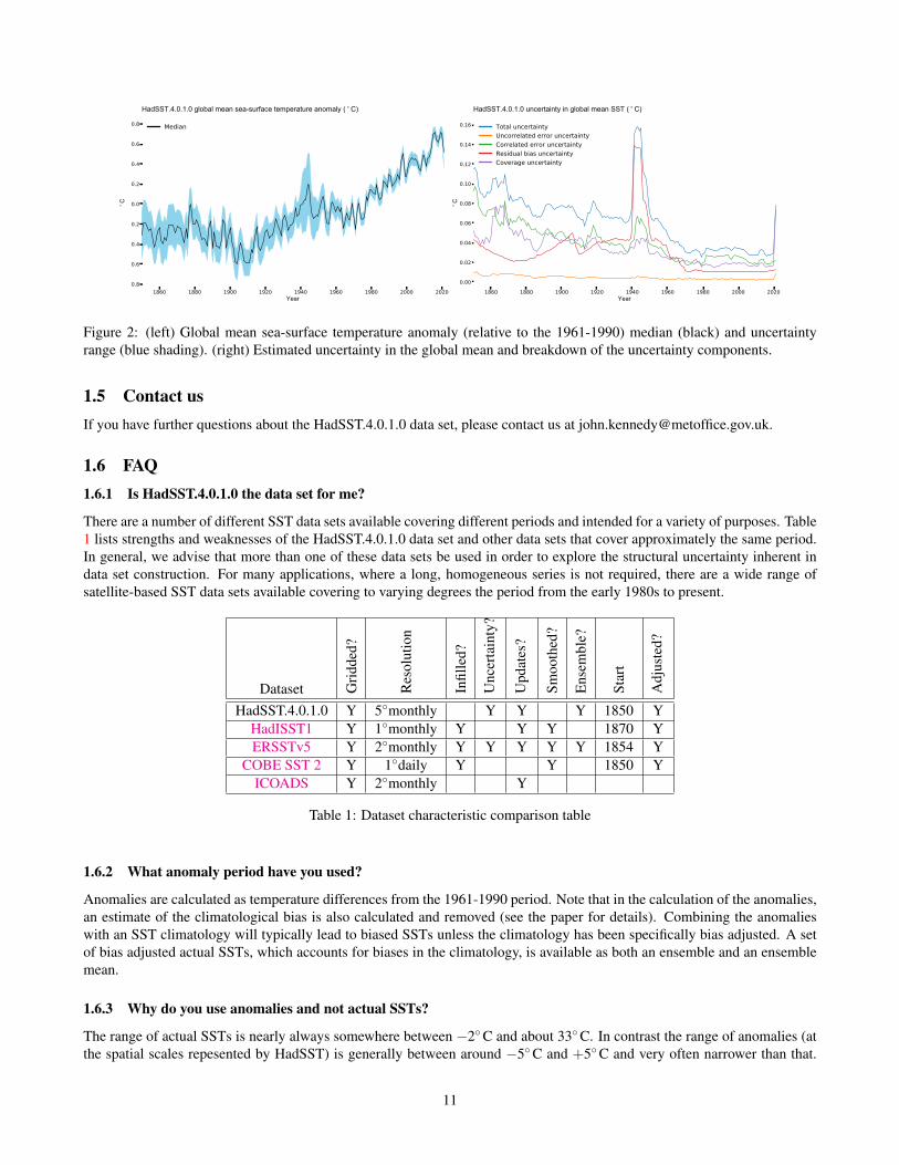
1.4 Basic data statisticsSome simple diagnostics are shown in Figure 1. The number of SST observations has increased from around 2 to 12 thousandper month in the period 1850-1880 to between 0.5 and 1.8 million per month in the period 2000-present. The number ofsuper-observations (which counts the number of 1 degree 5 day grid cells containing data) has also increased over the sameperiod. However, in contrast to straight counts of observations, the number of super observations peaked between 1965 and1990 when the VOS fleet was at its peak. There are drops in the numbers of observations and super observations during bothWorld Wars. There is a seasonal cycle in the number of observations, with more during northern hemisphere summer months.In particular, August has large numbers of observations. This is partly due to the extra pentad in August (the year is split into12 pseudo months each comprising 6 5-day pentads, except August which has 7).

Figure 2 shows the global mean SST and its uncertainty along with a breakdown of the uncertainty into individual com-ponents. The overall change in global mean SST is a long-term increase. There were two periods of more rapid warming- 1900-1940 and 1975-present - separated by a period with little change in temperature 1945-1975. Uncertainties typicallyget larger the further back in time one goes. The major exception to this general rule is the period of the Second WorldWar where uncertainties are estimated to be much higher because of reduced shipping and undocumented changes in the waymeasurements were made.

10

1860 1880 1900 1920 1940 1960 1980 2000 2020Year

−0.8

−0.6

−0.4

−0.2

0.0

0.2

0.4

0.6

0.8∘C

HadSST.4.0.1.0 global mean sea-surface temperature anomaly ( ∘C)

∘edian

1860 1880 1900 1920 1940 1960 1980 2000 2020Year

0.00

0.02

0.04

0.06

0.08

0.10

0.12

0.14

0.16

∘C

HadSST.4.0.1.0 uncertainty in global mean SST ( ∘C)

Total∘uncertaintyUncorrelated∘error∘uncertaintyCorrelated∘error∘uncertaintyResidual∘bias∘uncertaintyCoverage∘uncertainty

Figure 2: (left) Global mean sea-surface temperature anomaly (relative to the 1961-1990) median (black) and uncertaintyrange (blue shading). (right) Estimated uncertainty in the global mean and breakdown of the uncertainty components.

1.5 Contact usIf you have further questions about the HadSST.4.0.1.0 data set, please contact us at john.kennedy@metoffice.gov.uk.

1.6 FAQ1.6.1 Is HadSST.4.0.1.0 the data set for me?

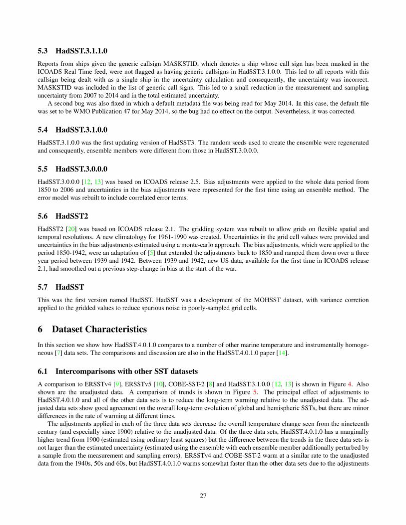
There are a number of different SST data sets available covering different periods and intended for a variety of purposes. Table1 lists strengths and weaknesses of the HadSST.4.0.1.0 data set and other data sets that cover approximately the same period.In general, we advise that more than one of these data sets be used in order to explore the structural uncertainty inherent indata set construction. For many applications, where a long, homogeneous series is not required, there are a wide range ofsatellite-based SST data sets available covering to varying degrees the period from the early 1980s to present.

Dataset Gri

dded

?

Res

olut

ion

Infil

led?

Unc

erta

inty

?

Upd

ates

?

Smoo

thed

?

Ens

embl

e?

Star

t

Adj

uste

d?

HadSST.4.0.1.0 Y 5◦monthly Y Y Y 1850 YHadISST1 Y 1◦monthly Y Y Y 1870 YERSSTv5 Y 2◦monthly Y Y Y Y Y 1854 Y

COBE SST 2 Y 1◦daily Y Y 1850 YICOADS Y 2◦monthly Y

Table 1: Dataset characteristic comparison table

1.6.2 What anomaly period have you used?

Anomalies are calculated as temperature differences from the 1961-1990 period. Note that in the calculation of the anomalies,an estimate of the climatological bias is also calculated and removed (see the paper for details). Combining the anomalieswith an SST climatology will typically lead to biased SSTs unless the climatology has been specifically bias adjusted. A setof bias adjusted actual SSTs, which accounts for biases in the climatology, is available as both an ensemble and an ensemblemean.

1.6.3 Why do you use anomalies and not actual SSTs?

The range of actual SSTs is nearly always somewhere between −2◦ C and about 33◦ C. In contrast the range of anomalies (atthe spatial scales repesented by HadSST) is generally between around −5◦ C and +5◦ C and very often narrower than that.

11

Because HadSST is a non-infilled data set, it is necessary to account for empty grid cells when calculating area averages.This is done by including a “coverage” uncertainty when area-averages are calculated. The coverage uncertainty is far smallerwhen using anomalies than it is when using actual SSTs. In addition, systematic gaps in observational coverage such as thoseat high-latitudes, where seasonal and permanent sea ice make measurement difficult, can lead to large biases in averages ofactual SSTs. Although systematic gaps in coverage can also affect averages based on SST anomalies, the effects are typicallymuch, much smaller.

Anomalies are also useful at other stages in processing. For example, during quality control, subtracting the climatologicalaverage from each SST measurement can reveal individual outliers. The largest difference between two good-quality obser-vations that are close to each other is often due to the climatological average difference in temperature at those two points.By accounting for the climatological difference between the locations of measurements when taking the difference betweennearby observations (equivalent to taking the difference of anomalies) it is often possible to identify more subtle errors in thedata.

When observations are averaged onto a regular grid, anomalies typically yield smaller uncertainties unless methods areused that account for the gradients of SST across the grid cell. Even then, using a climatology based on a large number ofobservations can still yield smaller uncertainties and a more reliable average.

Files containing gridded actual SSTs are available. These are constructed by adding the monthly grid-box average anomalyto a grid-box average climatology. Although they are required for some applications, users are reminded of the more pro-nounced effect that missing data have when using actual SSTs.

1.6.4 Where do the observations come from?

Individual SST reports are sourced from the International Comprehensive Ocean-Atmosphere Data Set (ICOADS) release3.0.0 (1850-2014) and 3.0.1 (2015-present). In addition, drifting buoy data were obtained from the Copernicus project. FromJanuary 2016 onwards, the Copernicus drifting buoys were used in place of the drifting buoys in ICOADS.3.0.1. ICOADScomprises a diverse range of data sources, provided in a consistent format with extensive (though incomplete) metadata.

International Comprehensive Ocean-Atmosphere Data Set (ICOADS) Release 3, Individual Observations. Research DataArchive at the National Center for Atmospheric Research, Computational and Information Systems Laboratory.

Drifting buoy data were collected and made freely available by the Copernicus project and the programs that contribute toit. Data downloaded from here.

In addition subsurface profile data from HadIOD.1.2.0.0 were used as reference data set for the calculation of the biasadjustments.

1.6.5 How does HadSST.4.0.1.0 differ from HadSST.3.0.0.0 and HadISST?

Key differences between different generations of HadSST and HadISST are summarized in Table 2. Note that HadSST.4.0.1.0is the recommended member of the HadSST family for current use.

1.6.6 Why are there 200 different data sets?

The 200 data sets are known as ’the ensemble’. The differences between the members of ’the ensemble’ represent uncertain-ties in the bias adjustment scheme. The errors associated with residual biases have complex long-term correlations and anensemble is the only practical way to express them. Briefly, uncertain parameters in the bias adjustment algorithm are variedwithin their plausible ranges to generate a range of different bias adjustments. Some of the uncertain parameters are thingslike what fraction of measurements with no metadata are assigned to particular measurement types. More details are given inthe paper.

1.6.7 What restrictions are there on the data? What is the data license?

The data and products are made available under the Open Government License v3.

1.6.8 How to acknowledge and cite the data?

We recommend that users of the data specify which version of the data set they used, when the data were downloaded, providea link to the website and a link to the license. For example:

12

HadSST.4.0.1.0 HadSST.3.1.1.0 HadSST2 HadISST1.1Resolution Monthly, 5◦ Monthly, 5◦ Monthly, 5◦ Monthly, 1◦

Time span 1850-present 1850-2018 1850-2014 1870-presentBase data set ICOADS.3.0.0 ICOADS.2.5.1 ICOADS.2.1 Met Office Marine

Data BankSatellite data

usedPartly: satellite dataare used to estimate

covariance structures

No No Yes

Datacompleteness

Gaps where there areno data

Gaps where there areno data

Gaps where there areno data

Globally complete

Data processing Simple gridding Simple gridding Simple gridding EOF-basedreconstruction

Bias adjustments Yes, 1850-present,space- and

time-varying ERIadjustment, buoy-ship

adjustment

Yes, 1850-present,fixed ERI adjustment,buoy-ship adjustment

Yes, 1850-1941,bucket corrections only

Yes, 1870-1941,bucket corrections only

Uncertainty ensemble + errorcovariance + fields

ensemble +fields fields none

Citation [14] [12, 13] [20] [21]Known issues See section 6.4 Recent trends are

underestimatedbecause of assumedconstant ERI bias

No bias adjustmentsafter 1941

No bias adjustmentsafter 1941, suspectedcold bias from late

1990s onwards

Table 2: Comparison with earlier versions of HadSST and HadISST.

HadSST.4.0.1.0 data were obtained from http://www.metoffice.gov.uk/hadobs/hadsst4/data on [date downloaded]and are ©British Crown Copyright, Met Office [year of download] provided under an Open Government Licensev3 http://www.nationalarchives.gov.uk/doc/open-government-licence/version/3/.

In addition, users of HadSST.4.0.1.0 are kindly requested to cite the specific journal article:

Kennedy, J.J., Rayner, N.A., Atkinson, C.P., and Killick, R.E. (2019). An ensemble data set of sea surfacetemperature change from 1850: the Met Office Hadley Centre HadSST.4.0.0.0 data set. Journal of GeophysicalResearch: Atmospheres, 124. https://doi.org/10.1029/2018JD029867.

1.6.9 There are gaps in the data, what can I do?

It is possible to process data with gaps in, but the gaps must be considered during the processing. For example, whencomparing datasets, it can be helpful to reduce the data sets to their common coverage so that a direct comparison can bemade. If you are using the actual SSTs instead of SST anomalies, you need to be extra careful how you deal with missingdata.

There are alternative products that you can use, in which the gaps have been filled by various methods. Long-term analysesinclude HadISST1 ([21]), ERSSTv5 ([10]) and COBE-SST-2 ([8]). There are a large number of analyses that cover the satelliteera including the SST CCI analysis product. One thing to note about infilled products is that there are still areas where thedata are more uncertain either due to lack of observations or because of limitations of the infilling techniques. Some recentpapers comparing different data sets and their uncertainties are [16, 15].

1.6.10 What do the different parts of the version number mean in HadSST.4.0.1.0?

The four components of the version number in HadSST.W.X.Y.Z are:

• W represents a major update which would usually be accompanied by a peer-reviewed publication. For example, thechange from HadSST.3.1.1.0 to HadSST.4.0.0.0 involved fundamental changes in the way that the bias adjustments

13

were calculated. A major version change would normally mean that users might want to, or indeed, need to, reconsiderhow they use the data.

• X represents a minor update, which would not normally require a peer-reviewed publication, but does affect muchof the record. For example, the change from HadSST.3.0.0.0 to HadSST.3.1.0.0 involved drawing new seeds for therandom numbers used to generate the ensemble. A minor version change would normally mean that users would needto redownload the whole data set.

• Y represents a very minor update, which would not normally require a peer-reviewed publication. This would be the kindof change that affected a few months of data, or made a negligible change to the whole record. For example, the changefrom HadSST.3.1.0.0 to HadSST.3.1.1.0 reduced the size of the smallest component of the estimated uncertainties forseven years at the end of the record. It also involved a bug fix in the code that made no difference to the output. A veryminor update of this kind would normally mean that users would need to redownload the whole data set to get all thefixes.

• Z is not currently used, but is kept for consistency with other Met Office Hadley Centre products.

1.6.11 When should I use the total uncertainty and when should I use the uncertainty components?

It will depend very much on your application, but in general a complete uncertainty calculation wil require use of the individualcomponents. The total uncertainty represents a combination of errors that correlate in very different ways so there is no wayto propagate the total uncertainty correctly. If you need to propagate the uncertainty, you will only be able to do this by usingthe individual components separately.

1.6.12 Why do the anomalies not average to zero in the climatology period?

The climatology used to calculate anomalies is spatially complete and represents the full annual cycle. This is achieved bycombining observations with interpolation as described in [20]. In some places coverage of observations during the 1961-1990climatology period is very sparse so the climatology is estimated from observations in a wider region. As a result of this, wedo not expect the available observations expressed as anomalies to exactly average to zero over the period 1961-1990.

2 Using the time series filesThe time series data and products are available under the Open Government License v3.

2.1 File namesThe filenames for the time series files follow a simple pattern: HadSST.4.0.1.0_annual_RRRR.csv where RRRR is the regionidentifier. The regions are described in the following table.

Region (RRRR) Nice name lat-lon extents W,S,E,NGLOBE Globe -180, -90, 180, 90SHEM Southern Hemisphere -180, -90, 180, 0NHEM Northern Hemisphere -180, 0, 180, 90TROP Tropics -180, -20, 180, 20

2.2 Tools that can be usedCSV files are simple text files and can be opened and read by any software that can process simple text files. They can beread and processed by a large number of different tools including Excel and Libre Open Office. In Python there are dedicatedstandard csv file readers as well as a number of packages, such as pandas, that can read and process CSV.

14

2.3 Contents of the time series filesThe files are csv (Comma Separated Value) files and the columns are described in the following Table.

Column Name Description; variable type Unitsyear Year; integer

month Month; integeranomaly SST anomaly relative to 1961-1990; floating point K

total_uncertainty Uncertainty combining all sources of uncertainty: uncorrelatedmeasurement error, sampling error, correlated measurement error

and residual bias uncertainty; floating point

K

uncorrelated_uncertainty 1σ Uncertainty from uncorrelated measurement errors and samplingerrors; floating point

K

correlated_uncertainty 1σ Uncertainty arising from correlated measurement errors; floatingpoint

K

bias_uncertainty 1σ residual bias uncertainty; floating point Kcoverage_uncertainty 1σuncertainty arising from errors due to large-scale coverage

limitations; floating pointK

lower_bound_95pct_bias_uncertainty_range 2.5%limit of the ensemble spread; floating point Kupper_bound_95pct_bias_uncertainty_range 97.5% limit of the ensemble spread; floating point K

3 Using the gridded data filesThe gridded data and products are available under the Open Government License v3.

3.1 File namesFilenames for the different data types are given in the following table.

15

Filename Sec. Variable NotesHadSST.4.0.1.0_median.nc 3.3.1 SST anomaly Median of the 200 member ensemble

HadSST.4.0.1.0_unadjusted.nc 3.3.2 SST anomaly Unadjusted, biased SST anomaliesHadSST.4.0.1.0_ensemble_member_EEEE.nc 3.3.3 SST anomaly EEEE is the ensemble number in the

range [1,200]HadSST.4.0.1.0_actuals_median.nc 3.3.4 SST actual Median of the 200 member ensemble

HadSST.4.0.1.0_actuals_ensemble_member_EEEE.nc 3.3.5 SST actual EEEE is the ensemble number in therange [1,200]

HadSST.4.0.1.0_number_of_observations.nc 3.3.6 Ob count Number of observations contributingto grid cell averages

HadSST.4.0.1.0_number_of_superobservations.nc 3.3.7 Ob count Number of superobservationscontributing to grid cell averages

HadSST.4.0.1.0_total_uncertainty.nc 3.3.8 Uncertainty Combined uncertainty in the grid cellaverage SST anomaly including

uncertainties associated with residualbias errors, uncorrelated measurementerrors, correlated measurement errors

and samplingHadSST.4.0.1.0_measurement_and_sampling_uncertainty.nc 3.3.9 Uncertainty Combined uncertainty in the grid cell

average SST anomaly includinguncertainties associated with

uncorrelated measurement errors,correlated measurement errors andsampling. This does NOT include

uncertainty associated with residualbiases.

HadSST.4.0.1.0_uncorrelated_measurement_uncertainty.nc 3.3.10 Uncertainty Uncertainty arising from uncorrelatedmeasurement errors

HadSST.4.0.1.0_correlated_measurement_uncertainty.nc 3.3.11 Uncertainty Uncertainty arising from correlatedmeasurement errors

HadSST.4.0.1.0_sampling_uncertainty.nc 3.3.12 Uncertainty Uncertainty arising from samplingerrors

HadSST.4.0.1.0_fractional_contribution_bucket.nc 3.3.13 Ob count Fractional contribution of bucketobservations to the grid cell average.

HadSST.4.0.1.0_fractional_contribution_eri.nc 3.3.14 Ob count Fractional contribution of ERIobservations to the grid cell average.

HadSST.4.0.1.0_fractional_contribution_hull.nc 3.3.15 Ob count Fractional contribution of HULLobservations to the grid cell average.

HadSST.4.0.1.0_fractional_contribution_unknown.nc 3.3.16 Ob count Fractional contribution ofUNKNOWN observations to the grid

cell average.HadSST.4.0.1.0_fractional_contribution_drifter.nc 3.3.17 Ob count Fractional contribution of DRIFTER

observations to the grid cell average.HadSST.4.0.1.0_fractional_contribution_moored.nc 3.3.18 Ob count Fractional contribution of MOORED

observations to the grid cell average.

3.2 Tools that can be used to work with data filesA list of software tools that work with NetCDF files is maintained by UCAR https://www.unidata.ucar.edu/software/netcdf/software.html).Some simple tools for viewing and manipulating NetCDF files in Linux include:

• ncdump: provided with the NetCDF library, produces a text rendering of a NetCDF file (Unidata at UCAR).

• Climate Data Operators (CDO)s: a set of command line utilities for performing operations on NetCDF files including

16

concatenation, editing and mathematics (https://code.mpimet.mpg.de/projects/cdo).

• ncview: a program to produce graphical displays of the contents of NetCDF files. More information can be found here.A more complete list can be found here.

In addition, packages are available in most commonly-used scientific programming languages for reading and working withNetCDF files. For example, in Python there are numerous packages including:

• netCDF4 - this basic package provides functionality to read NetCDF files and extract metadata.

• Iris - developed by the Met Office, Iris provides functionality to read, write and process files in a variety of formatsincluding NetCDF. Some example snippets of code using Iris to process HadSST.4.0.1.0 are provided in Section 4.

There are a number of packages in R that can be used to process NetCDF files:

• ncdf4: https://cran.r-project.org/web/packages/ncdf4/index.html

• raster: https://cran.r-project.org/web/packages/raster/index.html

• rcdo: https://github.com/r4ecology/rcdo

• RNetCDF: https://cran.r-project.org/web/packages/RNetCDF/index.html

• CM SAF R tools: https://www.mdpi.com/2220-9964/8/3/109

3.3 Contents of data filesEach of the regular NetCDF file contains metadata and data. The metadata are compliant with the CF-1.5 convention. The ma-jority of files have the same basic structure with the following coordinates (The exception are the error covariances describedin Section 3.3.19).

coordinate size Description Notestime unlimited days since 1850-01-01T00:00:00Z

gregorian calendarStart and end dates for each

month are stored in time_bndslatitude 36 degrees_north Grid cell boundaries are

stored in latitude_bndslongitude 72 degrees_east Grid cell boundaries are

stored in longitude_bnds

3.3.1 SST anomalies: HadSST.4.0.1.0_median.nc

This file contains the median SST anomalies The variable names and attributes are given in the following table

Variable:attribute Value Notestos:standard_name sea_water_temperature_anomaly

tos:long_name Sea water temperature anomaly at adepth of 20cm

tos:var_name tostos:units K

global:title Ensemble-median sea-surfacetemperature anomalies from the

HadSST.4.0.1.0 data set

17

3.3.2 SST anomalies: HadSST.4.0.1.0_unadjusted.nc

This file contains the unadjusted SST anomalies The variable names and attributes are given in the following table

Variable:attribute Value Notestos:standard_name sea_water_temperature_anomaly

tos:long_name Unadjusted, biased sea watertemperature anomaly at a depth of

20cmtos:var_name tos

tos:units Kglobal:title Unadjusted, biased sea-surface

temperature anomalies from theHadSST.4.0.1.0 data set

3.3.3 SST anomalies: HadSST.4.0.1.0_ensemble_member_EEEE.nc

The 200 ensemble members are stored in a zip file. Unzipping the file produces 200 data sets in the same format. The filescontain the ensemble of SST anomaly data sets, where EEEE is the ensemble member number running from 1 to 200 Thevariable names and attributes are given in the following table

Variable:attribute Value Notestos:standard_name sea_water_temperature_anomaly

tos:long_name Sea water temperature anomaly at adepth of 20cm

tos:var_name tostos:units K

global:title Single ensemble member ofsea-surface temperature anomaliesfrom the HadSST.4.0.1.0 data set

3.3.4 SST actuals: HadSST.4.0.1.0_actuals_median.nc

This files contains the median actual SST. Actual SSTs are calculated by adding the bias adjusted anomalies to the biasadjusted climatology. Note that extra care is needed when using the actual SSTs as missing data have a much greater effecton area averages than is the case for anomalies. The variable names and attributes are given in the following table

Variable:attribute Value Notestos:standard_name sea_water_temperature

tos:long_name Sea water temperature at a depth of20cm

tos:var_name tostos:units K

global:title Ensemble-median sea-surfacetemperature from the HadSST.4.0.1.0

data set

3.3.5 SST actuals: HadSST.4.0.1.0_actuals_ensemble_member_EEEE.nc

The 200 ensemble members are stored in a zip file. Unzipping the file produces 200 data sets in the same format. The filescontain the ensemble of SST data sets, where EEEE is the ensemble member number running from 1 to 200. Actual SSTs arecalculated by adding the bias adjusted anomalies to the bias adjusted climatology. Note that extra care is needed when usingthe actual SSTs as missing data have a much greater effect on area averages than is the case for anomalies. The variable namesand attributes are given in the following table

18

Variable:attribute Value Notestos:standard_name sea_water_temperature

tos:long_name Sea water temperature at a depth of20cm

tos:var_name tostos:units K

global:title Single ensemble member ofsea-surface temperature from the

HadSST.4.0.1.0 data set

3.3.6 SST anomalies: HadSST.4.0.1.0_number_of_observations.nc

This file contains the numbers of observations contributing the grid cell average SST anomalies. The variable names andattributes are given in the following table

Variable:attribute Value Notestos:standard_name None

tos:long_name Number of observations contributingto sea water temperature anomaly

tos:var_name numobstos:units 1

global:title Number of observations contributingto sea-surface temperature anomalies

from the HadSST.4.0.1.0 data set

3.3.7 SST anomalies: HadSST.4.0.1.0_number_of_superobservations.nc

This file contains the numbers of super-observations contributing the grid cell average SST anomalies. The variable namesand attributes are given in the following table

Variable:attribute Value Notestos:standard_name None

tos:long_name Number of superobservationscontributing to sea water temperature

anomalytos:var_name numsuperobs

tos:units 1global:title Number of superobservations

contributing to sea-surfacetemperature anomalies from the

HadSST.4.0.1.0 data set

3.3.8 SST anomalies: HadSST.4.0.1.0_total_uncertainty.nc

This file contains the total uncertainties, combining bias, measurement and sampling uncertainty in the SST anomalies. Thevariable names and attributes are given in the following table

19

Variable:attribute Value Notestos:standard_name sea_water_temperature_anomaly

standard_errortos:long_name one-sigma total uncertainty in sea

water temperature anomalytos:var_name tos_unc

tos:units Kglobal:title Total uncertainty in sea-surface

temperature anomalies from theHadSST.4.0.1.0 data set

3.3.9 SST anomalies: HadSST.4.0.1.0_measurement_and_sampling_uncertainty.nc

This file contains the uncertainties combining measurement and sampling uncertainty in the SST anomalies. It does notinclude uncertainty arising from residual biases that remain after adjustment. It is intended to be used in conjunction with theensemble. The variable names and attributes are given in the following table

Variable:attribute Value Notestos:standard_name sea_water_temperature_anomaly

standard_errortos:long_name one-sigma uncertainty associated with

measurement and sampling errors insea water temperature anomaly

tos:var_name tos_unctos:units K

global:title Measurement and samplinguncertainty in sea-surface temperature

anomalies from the HadSST.4.0.1.0data set

3.3.10 SST anomalies: HadSST.4.0.1.0_uncorrelated_measurement_uncertainty.nc

This file contains estimated uncertainties associated with uncorrelated measurement errors in the gridded SST anomalies. Thevariable names and attributes are given in the following table

Variable:attribute Value Notestos:standard_name sea_water_temperature_anomaly

standard_errortos:long_name one-sigma uncertainty associated with

uncorrelated measurement errors insea water temperature anomaly

tos:var_name tos_unctos:units K

global:title Uncorrelated measurement erroruncertainty in sea-surface temperature

anomalies from the HadSST.4.0.1.0data set

3.3.11 SST anomalies: HadSST.4.0.1.0_correlated_measurement_uncertainty.nc

This file contains estimated uncertainties associated with simply-correlated measurement errors in the gridded SST anomalies.Note that the error covariance matrices give a more complete description of this uncertainty component including spatialcovariance of the errors. The variable names and attributes are given in the following table

20

Variable:attribute Value Notestos:standard_name sea_water_temperature_anomaly

standard_errortos:long_name one-sigma uncertainty associated with

correlated measurement errors in seawater temperature anomaly

tos:var_name tos_unctos:units K

global:title Correlated measurement erroruncertainty in sea-surface temperature

anomalies from the HadSST.4.0.1.0data set

3.3.12 SST anomalies: HadSST.4.0.1.0_sampling_uncertainty.nc

This file contains estimated sampling uncertainties in the gridded SST anomalies. The variable names and attributes are givenin the following table

Variable:attribute Value Notestos:standard_name sea_water_temperature_anomaly

standard_errortos:long_name one-sigma uncertainty associated with

sampling errors in sea watertemperature anomaly

tos:var_name tos_unctos:units K

global:title Uncorrelated sampling erroruncertainty in sea-surface temperature

anomalies from the HadSST.4.0.1.0data set

3.3.13 SST anomalies: HadSST.4.0.1.0_fractional_contribution_bucket.nc

This file contains the fractional contribution of bucket observations to the grid cell average SST anomalies. The variablenames and attributes are given in the following table

Variable:attribute Value Notestos:standard_name None

tos:long_name Fractional contribution of bucketmeasurements to grid box average

tos:var_name bucketfractos:units 1

global:title Fraction of bucket observationscontributing to sea-surface

temperature anomalies from theHadSST.4.0.1.0 data set

3.3.14 SST anomalies: HadSST.4.0.1.0_fractional_contribution_eri.nc

This file contains the fractional contribution of ERI observations to the grid cell average SST anomalies. The variable namesand attributes are given in the following table

21

Variable:attribute Value Notestos:standard_name None

tos:long_name Fractional contribution of erimeasurements to grid box average

tos:var_name erifractos:units 1

global:title Fraction of ERI observationscontributing to sea-surface

temperature anomalies from theHadSST.4.0.1.0 data set

3.3.15 SST anomalies: HadSST.4.0.1.0_fractional_contribution_hull.nc

This file contains the fractional contribution of HULL observations to the grid cell average SST anomalies. The variablenames and attributes are given in the following table

Variable:attribute Value Notestos:standard_name None

tos:long_name Fractional contribution of hullmeasurements to grid box average

tos:var_name hullfractos:units 1

global:title Fraction of HULL observationscontributing to sea-surface

temperature anomalies from theHadSST.4.0.1.0 data set

3.3.16 SST anomalies: HadSST.4.0.1.0_fractional_contribution_unknown.nc

This file contains the fractional contribution of UNKNOWN observations to the grid cell average SST anomalies. The variablenames and attributes are given in the following table

Variable:attribute Value Notestos:standard_name None

tos:long_name Fractional contribution of unknownmeasurements to grid box average

tos:var_name unknownfractos:units 1

global:title Fraction of UNKNOWN observationscontributing to sea-surface

temperature anomalies from theHadSST.4.0.1.0 data set

3.3.17 SST anomalies: HadSST.4.0.1.0_fractional_contribution_drifter.nc

This file contains the fractional contribution of DRIFTER observations to the grid cell average SST anomalies. The variablenames and attributes are given in the following table

22

Variable:attribute Value Notestos:standard_name None

tos:long_name Fractional contribution of driftermeasurements to grid box average

tos:var_name drifterfractos:units 1

global:title Fraction of DRIFTER observationscontributing to sea-surface

temperature anomalies from theHadSST.4.0.1.0 data set

3.3.18 SST anomalies: HadSST.4.0.1.0_fractional_contribution_moored.nc

This file contains the fractional contribution of MOORED observations to the grid cell average SST anomalies. The variablenames and attributes are given in the following table

Variable:attribute Value Notestos:standard_name None

tos:long_name Fractional contribution of mooredmeasurements to grid box average

tos:var_name mooredfractos:units 1

global:title Fraction of MOORED observationscontributing to sea-surface

temperature anomalies from theHadSST.4.0.1.0 data set

3.3.19 Error covariances: HadSST.4.0.1.0_error_covariance_YYYYMM.nc

These files contain the error covariances describing the spatial covariance of the simply-correlated errors in the grid cellaverage SST anomalies. There is one error covariance matrix per month with YYYY referring to the year and MM to themonth. The coordinates are different from the other files and are given in the following table.

coordinate Description Noteslocation_index_1 location_index_1 The location index is an index

which assigns a unique valueto each of the 2592 5◦ grid

cells in the regular grids. Thelatitudes and longitudes of the

indices are given in thevariables latitude_vector_1

and longitude_vector_1location_index_2 location_index_2 The location index is an index

which assigns a unique valueto each of the 2592 5◦ grid

cells in the regular grids. Thelatitudes and longitudes of the

indices are given in thevariables latitude_vector_2

and longitude_vector_2

The location indices can be aligned with latitudes and longitudes within the other files using the Latitude_vector andlongitude_vector variables. The key variables and attributes are as follows:

23

Variable:attribute Value Notestos_cov:standard_name sea_water_temperature_anomaly

standard_errortos_cov:long_name Error covariance of sea water

temperature anomaly at a depth of20cm

tos_cov:units K2 (K2) This is Kelvin squared as theerror covariances are variancesrather than standard deviations

tos_cov:cell_methods Not specifiedglobal:title Error covariance of sea-surface

temperature anomalies from theHadSST.4.0.1.0 data set

4 Worked examples

4.1 Calculate global mean SST time seriesRead data and calculate a global mean SST anomaly series from 1850 to present using the Iris package in Python.

import irisimport numpy as npimport matplotlib.pyplot as pltimport iris.analysis.cartography

anoms = iris.load_cube(’HadSST .4.0.1.0 _median.nc ’)grid_areas = iris.analysis.cartography.area_weights(anoms)timeseries = anoms.collapsed([’longitude ’, ’latitude ’],

iris.analysis.MEAN , weights=grid_areas)

plt.plot(timeseries.data)plt.show()

4.2 Calculate monthly area average and uncertaintyRead anomalies and uncertainties and the ensemble and calculate the global average for January 1850 with an estimate of itsuncertainty.

import irisimport numpy as npimport matplotlib.pyplot as pltimport iris.analysis.cartography

anoms = iris.load_cube(’HadSST .4.0.1.0 _median.nc ’)

uncorrelated_unc = iris.load_cube(’HadSST .4.0.1.0 _uncorrelated_measurement_uncertainty.nc ’)sampling_unc = iris.load_cube(’HadSST .4.0.1.0 _sampling_uncertainty.nc ’)

covariance = iris.load_cube(’HadSST .4.0.1.0 _error_covariance_185001.nc ’)

#combine the uncorrelated -measurement -error and sampling uncertaintiesm_and_s_unc = uncorrelated_unc*uncorrelated_unc + sampling_unc*sampling_uncm_and_s_unc = iris.analysis.maths.exponentiate(m_and_s_unc , 0.5)

fill_value = -1e30

#extract latitudes to a 2-d array and convert to relative areaslatitude = anoms.coord(’latitude ’). pointslatitude_field = np.zeros ((36, 72))for i in range (0 ,36): latitude_field[i,:] = latitude[i]area_field = np.cos(latitude_field * np.pi / 180.)

24

#form a vector from the anomaly fieldanoms_1d = np.reshape(anoms.data [0 ,: ,:] ,(2592 ,1))anoms_1d = anoms_1d.data

#form a vector from the measurement and sampling uncertaintyunc_1d = np.reshape(m_and_s_unc.data [0 ,: ,:] ,(2592 ,1))unc_1d = unc_1d.data

#form a vector from the area fieldareas_1d = np.reshape(area_field.data ,(2592 ,1))

#where there are missing data in the anomaly field , set the areas to zeroareas_1d[anoms_1d == fill_value] = 0.0unc_1d[anoms_1d == fill_value] = 0.0anoms_1d[anoms_1d == fill_value] = 0.0

#convert the measurement and sampling uncertainty to a diagaonal covariance#matrix and add to the covariancecovariance2 = np.diag(np.reshape(unc_1d*unc_1d ,(2592)))covariance = covariance + covariance2

#turn the areas into gridcell weights for the area average calculationareas_1d = areas_1d/sum(areas_1d)

#calculate the area averagearea_average = sum(anoms_1d * areas_1d) / sum(areas_1d)area_average = area_average [0]

#calculate the uncertainty in the area average. Have to do this in two stages#using numpy matrix multiplicationarea_average_uncertainty_pre = np.matmul(covariance.data ,areas_1d)area_average_uncertainty_sq = np.matmul(np.matrix.transpose(areas_1d),

area_average_uncertainty_pre)area_average_uncertainty = np.sqrt(area_average_uncertainty_sq.data )[0][0]

#read ensemble and extract 1st timestep for each memberensemble = iris.load(’HadSST .4.0.1.0 _ensemble_member_ *.nc ’)for i in range (0 ,200): ensemble[i] = ensemble[i][0:1]

#calculate the global area average timeseries for each ensemble member#the time series only has one time step thoughensemble_gmt = np.zeros ((200))for i in range (0 ,200):

grid_areas = iris.analysis.cartography.area_weights(ensemble[i])ts = ensemble[i]. collapsed ([’longitude ’, ’latitude ’],

iris.analysis.MEAN , weights=grid_areas)ensemble_gmt[i] = ts.data [0]

bias_unc = np.std(ensemble_gmt)

area_average_uncertainty_sq += bias_unc*bias_uncarea_average_uncertainty = np.sqrt(area_average_uncertainty_sq.data )[0][0]

print(’Global mean Jan 1850: {:4.2f} +- {:4.2f}’.format(area_average ,area_average_uncertainty ))

5 Version historyThis section describes, briefly, differences between versions of HadSST up to HadSST.4.0.1.0.

5.1 HadSST.4.0.1.0Three changes were made in version HadSST.4.0.1.0.

25

Total (1-sigma)

1850 1900 1950 2000

0.00

0.05

0.10

0.15

0.20HadSST.4.0.0.0HadSST.4.0.1.0HadSST.3.1.1.0

Measurement and sampling (1-sigma)

1850 1900 1950 2000

0.00

0.05

0.10

0.15

0.20

Bias (1-sigma)

1850 1900 1950 2000

0.00

0.05

0.10

0.15

0.20

Coverage (1-sigma)

1850 1900 1950 2000

0.00

0.05

0.10

0.15

0.20

Figure 3: Uncertainty components from HadSST.4.0.0.0 (orange), 4.0.1.0 (grey) and 3.1.1.0 (blue) including total uncertainty(top left), measurement and sampling uncertainty (top right), bias uncertainty (bottom left) and coverage uncertainty (bottomright). The HadSST.4.0.0.0 coverage uncertainty is erroneously large. Note that the measurement and sampling uncertaintiesand the bias uncertainties are identical in versions 4.0.1.0 and 4.0.0.0 except for the final three months of 2020 so the grey lineoverlays the orange line almost completely, rendering it all but invisible.

1. October, November and December 2020 were rerun using CMEMS data, having been originally updated using NOAAOMSC (for drifter data) in HadSST.4.0.0.0.

2. There was a bug in the code used to calculate the coverage uncertainty in the time series files in HadSST.4.0.0.0, whichmeant that the uncertainties were too large. A displaced mask meant that some land areas were misidentified as icecovered ocean areas. This has now been fixed.

3. A “fill_value” was added to the NetCDF files, the absence of which was causing problems for some users.

5.2 HadSST.4.0.0.0This was a major update from HadSST.3.1.1.0, which involved changes in almost all aspects of the data set. These aredescribed in [14]. The bias adjustment method was changed in almost all aspects, with particularly important changes to theway that engine room biases and measurement methods were estimated. These changes affected the whole record in someway. The ensemble was expanded to 200 members. A more complete breakdown of uncertainty components was provided tousers, including error covariances that describe uncertainties associated with correlated errors. HadSST.4.0.0.0 was the firstHadSST data set to use ICOADS release 3.0.0 and 3.0.1 for updates.

October, November and December 2020 were updated using drifting buoy data from the NOAA OSMC service as impor-tant metadata identifying individual buoys was removed from the CMEMS drifter data files rendering them unusable. Thismetadata has since been reinstated and used to create HadSST.4.0.1.0 (see above).

26

5.3 HadSST.3.1.1.0Reports from ships given the generic callsign MASKSTID, which denotes a ship whose call sign has been masked in theICOADS Real Time feed, were not flagged as having generic callsigns in HadSST.3.1.0.0. This led to all reports with thiscallsign being dealt with as a single ship in the uncertainty calculation and consequently, the uncertainty was incorrect.MASKSTID was included in the list of generic call signs. This led to a small reduction in the measurement and samplinguncertainty from 2007 to 2014 and in the total estimated uncertainty.

A second bug was also fixed in which a default metadata file was being read for May 2014. In this case, the default filewas set to be WMO Publication 47 for May 2014, so the bug had no effect on the output. Nevertheless, it was corrected.

5.4 HadSST.3.1.0.0HadSST.3.1.0.0 was the first updating version of HadSST3. The random seeds used to create the ensemble were regeneratedand consequently, ensemble members were different from those in HadSST.3.0.0.0.

5.5 HadSST.3.0.0.0HadSST.3.0.0.0 [12, 13] was based on ICOADS release 2.5. Bias adjustments were applied to the whole data period from1850 to 2006 and uncertainties in the bias adjustments were represented for the first time using an ensemble method. Theerror model was rebuilt to include correlated error terms.

5.6 HadSST2HadSST2 [20] was based on ICOADS release 2.1. The gridding system was rebuilt to allow grids on flexible spatial andtemporal resolutions. A new climatology for 1961-1990 was created. Uncertainties in the grid cell values were provided anduncertainties in the bias adjustments estimated using a monte-carlo approach. The bias adjustments, which were applied to theperiod 1850-1942, were an adaptation of [5] that extended the adjustments back to 1850 and ramped them down over a threeyear period between 1939 and 1942. Between 1939 and 1942, new US data, available for the first time in ICOADS release2.1, had smoothed out a previous step-change in bias at the start of the war.

5.7 HadSSTThis was the first version named HadSST. HadSST was a development of the MOHSST dataset, with variance corretionapplied to the gridded values to reduce spurious noise in poorly-sampled grid cells.

6 Dataset CharacteristicsIn this section we show how HadSST.4.0.1.0 compares to a number of other marine temperature and instrumentally homoge-neous [7] data sets. The comparisons and discussion are also in the HadSST.4.0.1.0 paper [14].

6.1 Intercomparisons with other SST datasetsA comparison to ERSSTv4 [9], ERSSTv5 [10], COBE-SST-2 [8] and HadSST.3.1.0.0 [12, 13] is shown in Figure 4. Alsoshown are the unadjusted data. A comparison of trends is shown in Figure 5. The principal effect of adjustments toHadSST.4.0.1.0 and all of the other data sets is to reduce the long-term warming relative to the unadjusted data. The ad-justed data sets show good agreement on the overall long-term evolution of global and hemispheric SSTs, but there are minordifferences in the rate of warming at different times.

The adjustments applied in each of the three data sets decrease the overall temperature change seen from the nineteenthcentury (and especially since 1900) relative to the unadjusted data. Of the three data sets, HadSST.4.0.1.0 has a marginallyhigher trend from 1900 (estimated using ordinary least squares) but the difference between the trends in the three data sets isnot larger than the estimated uncertainty (estimated using the ensemble with each ensemble member additionally perturbed bya sample from the measurement and sampling errors). ERSSTv4 and COBE-SST-2 warm at a similar rate to the unadjusteddata from the 1940s, 50s and 60s, but HadSST.4.0.1.0 warms somewhat faster than the other data sets due to the adjustments

27

-1.0

-0.8

-0.6

-0.4

-0.2

-0.0

0.2

0.4

0.6

0.8 (a) Globe

-0.2-0.1 0.0 0.1 0.2

(b) difference

-1.0

-0.8

-0.6

-0.4

-0.2

-0.0

0.2

0.4

0.6

0.8 (c) Southern Hemisphere

-0.2-0.1 0.0 0.1 0.2

(d) difference

-1.0

-0.8

-0.6

-0.4

-0.2

-0.0

0.2

0.4

0.6

0.8 (e) Northern Hemisphere

-0.2-0.1 0.0 0.1 0.2

(f) difference

1900 1920 1940 1960 1980 2000 2020

Anom

aly

(oC

) re

lative to 1

961-1

990

Date produced: Thu Sep 23 18:26:32 BST 2021. From code revision:970

Figure 4: Updated from [14]. (a) (c) and (e) Global and regional average SST anomaly 1850-2012 (°C relative to 1961-1990) series from HadSST.4.0.1.0 (black), ERSSTv5 (blue, thick line is operational version and thin-thick dashed lines areensemble range from the 1000-member ERSSTv4 ensemble), COBE-SST-2 (orange), HadSST.3.1.1.0 (green) and unadjustedSSTs (red). The green line is HadSST.3.1.1.0. (b) (d) and (f) Differences from the HadSST.4.0.1.0 median. The grey shadingindicates the 95% uncertainty range for HadSST.4.0.1.0 including effects from measurement, sampling and bias-adjustmenterrors. The bias-adjustment uncertainty range is shown in darker grey. Colours for other lines are as in panels (a), (c) and (e).

28

-0.1

0.0

0.1

0.2

Tre

nd

(oC

/de

ca

de

)

19

00

19

10

19

20

19

30

19

40

19

50

19

60

19

70

19

80

19

90

20

00

(a) Globe

-0.1

0.0

0.1

0.2

Tre

nd

(oC

/de

ca

de

)

19

00

19

10

19

20

19

30

19

40

19

50

19

60

19

70

19

80

19

90

20

00

(b) Southern Hemisphere

-0.1

0.0

0.1

0.2

Tre

nd

(oC

/de

ca

de

)

19

00

19

10

19

20

19

30

19

40

19

50

19

60

19

70

19

80

19

90

20

00

(c) Northern Hemisphere

-0.1

0.0

0.1

0.2

0.3

0.4

Tre

nd

(oC

/de

ca

de

)

19

00

19

10

19

20

19

30

19

40

19

50

19

60

19

70

19

80

19

90

20

00

(d) North Atlantic

Date produced: Thu Sep 23 18:26:47 BST 2021. From code revision:970

Figure 5: Updated from [14]. Global and regional average SST anomaly trends to 2012. Median trends from HadSST.4.0.1.0are indicated by a black horizontal line and the grey shading indicates median and 95% uncertainty range including effectsfrom measurement, sampling and bias-adjustment errors. The bias-adjustment uncertainty range is shown in darker grey;ERSSTv5 (blue), the lozenge is the operational version and the vertical line is the 95% ensemble range from the 1000-memberERSSTv4 ensemble); COBE-SST-2 (orange); HadSST.3.1.1.0 (green); and unadjusted SSTs (red).

29

applied to account for the general decline in ERI biases over that period. From start dates in 1970, 1980 and 1990, COBE-SST-2 warms faster than the unadjusted data and, from 1980 and 1990, faster than either HadSST.4.0.1.0 or ERSSTv4 by asignificant margin.

From 2000-2012, the rates of warming in all three data sets are very similar and consistent within their uncertainty ranges.All three warm faster than the unadjusted data, which has a trend close to zero. During this period, there are two importantfactors. First, there is a large increase in the relatively cooler drifting buoy measurements and, second, there is a decrease inthe average ship bias. The analysis of HadSST.4.0.1.0 supports ERSSTv4 and ERSSTv5 in this period ([11]) and is consistentwith instrumentally homogeneous reference series, supporting the analysis of [7].

6.2 Comparison to other long recordsOver longer periods, it is necessary to use other data sets for comparison. We use two data sets here. The first is HadN-MAT.2.0.1.0 ([17]) which is a data set of Nighttime Marine Air Temperatures (NMAT). Anomalies in NMAT are thought toclosely track anomalies in SST over long periods and large scales (see [9] for an example using climate models). The secondis based on oceanographic profiles from HadIOD.1.2.0.0, excluding Argo ([1]) and adjusted using the [18] adjustments forMBTs and XBTs.

In order to make a direct comparison between HadSST.4.0.1.0 and HadIOD.1.2.0.0, anomalies from HadSST.4.0.1.0 wereadjusted using the absolute bias rather than the relative bias so that the SSTs could be directly compared. Anomalies were thencalculated for both data sets using an unadjusted climatology. However, HadSST.4.0.1.0 is not then directly comparable toHadNMAT.2.0.1.0 as HadNMAT.2.0.1.0 is provided as actuals or relative to its own adjusted 1961-1990 climatology and notrelative to a biased SST climatology. This will lead to a constant annual offset between the SST and NMAT series, which isapproximately the size of the average climatological bias in the SST. Consequently, we shifted HadNMAT.2.0.1.0 by 0.15°Cin Figure 6. The offset was chosen by eye to approximately align the two series; none of the conclusions depend on the choiceof offset.

Except for a period in the late 1940s and early 1950s, differences between HadNMAT.2.0.1.0 and HadSST.4.0.1.0 anoma-lies (Figure 13b) on a decadal time scale are constant between 1920 and 1990. Outside this period, the differences exceedthe estimated uncertainties in the HadSST.4.0.1.0 data set. One notable difference occurs around 1991-1993, when HadN-MAT.2.0.1.0 apparently cools relative to HadSST.4.0.0.0 (or HadSST.4.0.1.0 warms). Further investigation shows that thecooling occurs in the tropics, partly offset by warming in the northern extratropical Pacific.

6.3 Instrumentally homogeneous seriesInstrumentally homogeneous data sets [7] are data sets which comprise measurements from a single instrument, or standard-ised collection of instruments, chosen to be stable and accurate.

6.3.1 Argo

Argo floats are autonomous floating devices that make temperature profile measurements usually in the upper 2000m of thewater column. Argo floats float with the prevailing currents at a depth of 1000m. Every ten days, the float descends to2000m then rises to the surface measuring water temperatures along the way. An estimate of SST can be had by taking themeasurement nearest to the surface and above a specified depth, in this case 10m. The measurements made by Argo floats areconsidered to be accurate, with estimated uncertainties of hundredths of a degree or better. However, sampling is relativelysparse with each of the floats sampling the SST only once every 10 days. Nonetheless, the excellent coverage and low noise ofthe measurements means that a reasonably global average can be calculated from the observations from the mid 2000s. Dueto the careful calibration of the sensors, the series (aside from shifts in coverage) is expected to be reasonably stable.

Figure 7 shows a comparison between HadSST.4.0.1.0 and gridded Argo observations. The gridding was the same as wasused for HadSST.4.0.1.0. The adjustments applied to HadSST.4.0.1.0 bring the SST series into closer agreement with theArgo data.

6.3.2 ARC ATSR Reprocessing for Climate

Figure 7 also shows a comparison with the ARC ATSR Reprocessing for Climate[19] data set. The ATSR series of instrumentswere designed to take climate quality measurements. The excellent coverage of the dataset means that it is possible to assessHadSST.4.0.1.0 at a wide range of locations. Here we show the global average. The ARC v1.1 data were gridded using thesame method as for HadSST.4.0.1.0 to minimize inconsistencies that might arise from processing. Agreement between the

30

1900 1920 1940 1960 1980 2000

-0.8

-0.6

-0.4

-0.2

0.0

0.2

0.40.6

Ano

maly

(oC

)

(a) HadNMAT.2.0.1.0 and HadSST.4.0.1.0

1900 1920 1940 1960 1980 2000

-0.4

-0.2

0.0

0.2

0.4

Diffe

ren

ce (

oC

)

(b) HadNMAT.2.0.1.0 minus HadSST.4.0.1.0

1900 1920 1940 1960 1980 2000

-0.8

-0.6

-0.4

-0.2

0.0

0.2

0.40.6

An

om

aly

(oC

)

(c) HadIOD, HadNMAT.2.0.1.0 and HadSST.4.0.1.0

1900 1920 1940 1960 1980 2000

-0.4

-0.2

0.0

0.2

0.4

Ano

maly

(oC

)

(d) HadIOD, HadNMAT.2.0.1.0 minus HadSST.4.0.1.0

Date produced: Thu Sep 23 19:29:30 BST 2021. From code revision:970

Figure 6: From [14]. (a) Collocated global annual average NMAT anomalies (°C) 1900-2010 offset by 0.15°C (blue, relativeto 1961-1990) and global annual average SST anomalies from HadSST.4.0.1.0 (black is central estimate and grey shadingindicates 95% uncertainty range). (b) Offset NMAT anomalies minus SST anomalies with combined 95% uncertainty range(taking into account the bias errors from the HadSST.4.0.1.0 ensemble, and measurement and sampling errors in the SST).The dashed line indicates zero difference. (c) Collocated global annual average offset NMAT anomalies (blue), global annualaverage near-surface water temperature from HadIOD excluding Argo (orange) and SST (black is central estimate and greyshading again indicates 95% uncertainty range). (d) Difference between HadIOD and HadSST.4.0.1.0 (orange) and NMATand HadSST.4.0.1.0 (blue). The shaded area indicates the 95% uncertainty range..

31

-0.2

0.0

0.2

0.4

0.6

Anom

aly

(oC

)

(a) Argo

(b)

-0.2

0.0

0.2

0.4

0.6

An

om

aly

(oC

)

(c) ARC

(d)

-0.2

0.0

0.2

0.4

0.6

An

om

aly

(oC

)

(e) Buoys

1990 1995 2000 2005 2010 2015 2020

(f)

Date produced: Thu Sep 23 18:50:43 BST 2021. From code revision:970

Figure 7: From [14]. Comparison to instrumentally homogeneous data sets. (a) global average SST anomalies from Argo(purple) and HadSST.4.0.1.0 (black and grey shading). The dotted line shows a global average calculated from unadjusteddata. All comparisons are colocated. (b) coverage of HadSST.4.0.1.0 (grey) and coverage of the Argo data (purple). (c) and(d) as for (a) and (b) but for ARC data. (e) and (f) as for (a) and (b) but for drifting buoy data.

32

two data sets is good for most of the ATSR2 and AATSR records - roughly from 1995 to 2012. The short segment of datain 1991 was recorded by the ATSR1 instrument before the failure of one of the infra-red channels. The assessed quality ofthe ATSR1 SST retrievals is lower than for the ATSR2 and AATSR instruments. Note that there are regional biases betweenARC and HadSST.4.0.1.0 which are likely due to biases in the ARC retrievals, or subtle differences in the precise measurand.Similar differences are seen between ARC and drifting buoy data.

6.3.3 Buoys

The final panel in Figure 7 shows comparisons between buoy data and HadSST.4.0.1.0. The buoy data are used in the creationof HadSST.4.0.1.0, so this does not constitute validation of the dataset. However, it is important to note that the inclusion ofship data has not degraded the analysis. There is a divergence between the series in 1992/1993. This is a period of relativelylow buoy coverage. One thing to note is that the bias adjustments applied to HadSST.4.0.1.0 cool the ship data particularlybetween 1990 and 2010.

6.4 Known issues arising in the literatureAs time goes on, new research reveals previously unknown problems with the data. It is now always possible to incorporatethis information in data sets during regular updates. Nonetheless it can be important for users to be aware of the widerliterature. A number of studies have been published both during the HadSST.4.0.1.0 development and since its release whichhave potential impacts on understanding of the data set.

[2] used a probabilistic algorithm to assign marine reports to ship tracks. In HadSST.4.0.1.0 the error covariances areconstructed using only those observations that have a non-missing and non-generic call sign or ID. This means the error-covariances most likely under-estimate the simply-correlated part of the total uncertainty, particulary during periods, such asthe 1860s when few reports have valid IDs in ICOADS. Assigning reports with erroneous IDs, missing IDs or generic IDs(such as SHIP or MASK) to ship tracks would increase the number of reports that can be included in the error covariances.This has not yet been done.

[4, 3]showed that there are errors in the data that correlate at the level of individual decks in ICOADS (decks refer tothe decks of punched cards used to store and transmit the earliest digital data) or at a national level. However, there is noevidence that this affects trends in the global average. Uncertainties in HadSST.4.0.1.0 account for correlations at the level ofindividual ships and in large scale biases at a quasi-global level. Correlations at a deck or nation level would act to increasethe uncertainty above what is estimated in HadSST.4.0.1.0 at present. However, in the period after 1950, the majority of shipsuse engine room measurements and the spatially-temporally varying engine room adjustments in HadSST.4.0.1.0 will accountfor much of this inter-deck or inter-nation variation. Prior to 1950, because fixed fields are used for the bucket adjustments,there is no component of the analysis that accounts for uncertainty correlating at the deck or nation level. Consequently,the simply-correlated measurement errors will be under-estimated. An initial estimate assigning an uncertainty of 0.2◦C toindividual decks suggests an approximate doubling of the uncertainty due to simply-correlated uncertainties in the period from1850 to the start of the Second World War. However, this needs to be confirmed.

[4] also identified a cold bias in Japanese data from specific decks. This cold bias was due to truncation, rather thanrounding, of decimal temperatures. Consequently, it is likely that the mean of HadSST4 is too cold by a varying amount in theaffected period - roughly from the 1930s to the 1960s - with the largest effect in the North Pacific. Please refer to the papersfor more details.

6.5 Processing notesThis section covers topics that were not covered in the paper.

6.5.1 Coverage uncertainty

The calculation of coverage uncertainty - the uncertainty arising from having empty grid boxes when calculating an areaaverage - was not described in the HadSST.4.0.1.0 paper. Coverage uncertainty was added to the time series files after the dataset was released. The coverage uncertainty for a month was calculated as follows.

A missing data mask was created for the month. This mask was used to subsample every monthly field in HadISST1,which is otherwise a globally complete SST data set. A time series of HadISST SST anomalies was calculated from thesub-sampled fields and from the globally-complete fields. The root mean squared difference between these two was used asan estimate of the coverage uncertainty.

33

Note that this process differs from that described in the HadSST.3.0.0.0 paper in that the RMS difference is used ratherthan the standard deviation.

References[1] Christopher P. Atkinson, Nick A. Rayner, John J. Kennedy, and Simon A. Good. An integrated database of ocean tem-

perature and salinity observations. Journal of Geophysical Research: Oceans, 119(10):7139–7163, 2014. URL: https://agupubs.onlinelibrary.wiley.com/doi/abs/10.1002/2014JC010053, doi:10.1002/2014JC010053.

[2] Giulia Carella, Elizabeth C. Kent, and David I. Berry. A probabilistic approach to ship voyage reconstruction in icoads.International Journal of Climatology, pages n/a–n/a, 2015. URL: http://dx.doi.org/10.1002/joc.4492, doi:10.1002/joc.4492.

[3] Duo Chan and Peter Huybers. Systematic Differences in Bucket Sea Surface Temperature Measurements among NationsIdentified Using a Linear-Mixed-Effect Method. Journal of Climate, 32(9):2569–2589, May 2019. URL: http://journals.ametsoc.org/doi/10.1175/JCLI-D-18-0562.1, doi:10.1175/JCLI-D-18-0562.1.

[4] Duo Chan, Elizabeth C. Kent, David I. Berry, and Peter Huybers. Correcting datasets leads to more homogeneous early-twentieth-century sea surface warming. Nature, 571(7765):393–397, July 2019. URL: http://www.nature.com/articles/s41586-019-1349-2, doi:10.1038/s41586-019-1349-2.

[5] C.K. Folland and D.E. Parker. Correction of instrumental biases in historical sea surface temperature data. QuarterlyJournal of the Royal Meteorological Society, 121(522):319–367, 1995. doi:10.1002/qj.49712152206.

[6] Eric Freeman, Scott D. Woodruff, Steven J. Worley, Sandra J. Lubker, Elizabeth C. Kent, William E. An-gel, David I. Berry, Philip Brohan, Ryan Eastman, Lydia Gates, Wolfgang Gloeden, Zaihua Ji, Jay Lawrimore,Nick A. Rayner, Gudrun Rosenhagen, and Shawn R. Smith. Icoads release 3.0: a major update to the his-torical marine climate record. International Journal of Climatology, 37(5):2211–2232, 2017. URL: https://rmets.onlinelibrary.wiley.com/doi/abs/10.1002/joc.4775, arXiv:https://rmets.onlinelibrary.wiley.com/doi/pdf/10.1002/joc.4775, doi:10.1002/joc.4775.

[7] Zeke Hausfather, Kevin Cowtan, David C. Clarke, Peter Jacobs, Mark Richardson, and Robert Rohde. Assessing recentwarming using instrumentally homogeneous sea surface temperature records. Science Advances, 3(1), 2017. URL:https://advances.sciencemag.org/content/3/1/e1601207, arXiv:https://advances.sciencemag.org/content/3/1/e1601207.full.pdf, doi:10.1126/sciadv.1601207.

[8] Shoji Hirahara, Masayoshi Ishii, and Yoshikazu Fukuda. Centennial-scale sea surface temperature analysis and itsuncertainty. Journal of Climate, 27(1):57–75, 2014. URL: https://doi.org/10.1175/JCLI-D-12-00837.1, doi:10.1175/JCLI-D-12-00837.1.

[9] Boyin Huang, Viva F Banzon, Eric Freeman, Jay Lawrimore, Wei Liu, Thomas C Peterson, Thomas M Smith, Peter WThorne, Scott D Woodruff, and Huai-Min Zhang. Extended reconstructed sea surface temperature version 4 (ersst. v4).part i: Upgrades and intercomparisons. Journal of Climate, 28(3):911–930, 2015. URL: https://doi.org/10.1175/JCLI-D-14-00006.1, doi:10.1175/JCLI-D-14-00006.1.

[10] Boyin Huang, Peter W. Thorne, Viva F. Banzon, Tim Boyer, Gennady Chepurin, Jay H. Lawrimore, Matthew J. Menne,Thomas M. Smith, Russell S. Vose, and Huai-Min Zhang. Extended reconstructed sea surface temperature, version 5(ersstv5): Upgrades, validations, and intercomparisons. Journal of Climate, 30(20):8179–8205, 2017. URL: https://doi.org/10.1175/JCLI-D-16-0836.1, doi:10.1175/JCLI-D-16-0836.1.

[11] Thomas R. Karl, Anthony Arguez, Boyin Huang, Jay H. Lawrimore, James R. McMahon, Matthew J. Menne, Thomas C.Peterson, Russell S. Vose, and Huai-Min Zhang. Possible artifacts of data biases in the recent global surface warming hia-tus. Science, 348(6242):1469–1472, 2015. URL: https://science.sciencemag.org/content/348/6242/1469,doi:10.1126/science.aaa5632.

[12] J. J. Kennedy, N. A. Rayner, R. O. Smith, D. E. Parker, and M. Saunby. Reassessing biases and other uncertainties in seasurface temperature observations measured in situ since 1850: 1. measurement and sampling uncertainties. Journal ofGeophysical Research: Atmospheres, 116(D14), 2011. URL: https://agupubs.onlinelibrary.wiley.com/doi/abs/10.1029/2010JD015218, doi:10.1029/2010JD015218.

34

[13] J. J. Kennedy, N. A. Rayner, R. O. Smith, D. E. Parker, and M. Saunby. Reassessing biases and other uncertainties insea surface temperature observations measured in situ since 1850: 2. biases and homogenization. Journal of Geophysi-cal Research: Atmospheres, 116(D14), 2011. URL: https://agupubs.onlinelibrary.wiley.com/doi/abs/10.1029/2010JD015220, doi:10.1029/2010JD015220.

[14] J.J. Kennedy, N.A. Rayner, C.P. Atkinson, and R.E. Killick. An ensemble data set of sea-surface temperature changefrom 1850: the Met Office Hadley Centre HadSST.4.0.0.0 data set. Journal of Geophysical Research: Atmospheres,2019.

[15] John J. Kennedy. A review of uncertainty in in situ measurements and data sets of sea surface temperature. Re-views of Geophysics, 52(1):1–32, 2014. URL: https://agupubs.onlinelibrary.wiley.com/doi/abs/10.1002/2013RG000434, doi:10.1002/2013RG000434.

[16] Elizabeth C. Kent, John J. Kennedy, Thomas M. Smith, Shoji Hirahara, Boyin Huang, Alexey Kaplan, David E. Parker,Christopher P. Atkinson, David I. Berry, Giulia Carella, Yoshikazu Fukuda, Masayoshi Ishii, Philip D. Jones, FinnLindgren, Christopher J. Merchant, Simone Morak-Bozzo, Nick A. Rayner, Victor Venema, Souichiro Yasui, and Huai-Min Zhang. A call for new approaches to quantifying biases in observations of sea surface temperature. Bulletin of theAmerican Meteorological Society, 98(8):1601–1616, 2017. doi:10.1175/BAMS-D-15-00251.1.

[17] Elizabeth C. Kent, Nick A. Rayner, David I. Berry, Michael Saunby, Bengamin I. Moat, John J. Kennedy, and David E.Parker. Global analysis of night marine air temperature and its uncertainty since 1880: The hadnmat2 data set. Journal ofGeophysical Research: Atmospheres, 118(3):1281–1298, 2013. URL: https://agupubs.onlinelibrary.wiley.com/doi/abs/10.1002/jgrd.50152, doi:10.1002/jgrd.50152.

[18] S. Levitus, J. I. Antonov, T. P. Boyer, R. A. Locarnini, H. E. Garcia, and A. V. Mishonov. Global ocean heat content 1955-2008 in light of recently revealed instrumentation problems. Geophysical Research Letters, 36(7), 2009. URL: https://agupubs.onlinelibrary.wiley.com/doi/abs/10.1029/2008GL037155, doi:10.1029/2008GL037155.

[19] Christopher J. Merchant, Owen Embury, Nick A. Rayner, David I. Berry, Gary K. Corlett, Katie Lean, Karen L. Veal,Elizabeth C. Kent, David T. Llewellyn-Jones, John J. Remedios, and Roger Saunders. A 20Â year independent record ofsea surface temperature for climate from along-track scanning radiometers. Journal of Geophysical Research: Oceans,117(C12), 2012. URL: https://agupubs.onlinelibrary.wiley.com/doi/abs/10.1029/2012JC008400, doi:10.1029/2012JC008400.

[20] N. A. Rayner, P. Brohan, D. E. Parker, C. K. Folland, J. J. Kennedy, M. Vanicek, T. J. Ansell, and S. F. B. Tett. Improvedanalyses of changes and uncertainties in sea surface temperature measured in situ since the mid-nineteenth century: TheHadSST2 dataset. Journal of Climate, 19(3):446–469, 2006. doi:10.1175/JCLI3637.1.

[21] N. A. Rayner, D. E. Parker, E. B. Horton, C. K. Folland, L. V. Alexander, D. P. Rowell, E. C. Kent, and A. Kaplan. Globalanalyses of sea surface temperature, sea ice, and night marine air temperature since the late nineteenth century. Journalof Geophysical Research: Atmospheres, 108(D14), 2003. URL: https://agupubs.onlinelibrary.wiley.com/doi/abs/10.1029/2002JD002670, arXiv:https://agupubs.onlinelibrary.wiley.com/doi/pdf/10.1029/2002JD002670, doi:10.1029/2002JD002670.

35