arX

iv:h

ep-e

x/99

0403

2v1

29

Apr

199

9EUROPEAN ORGANIZATION FOR NUCLEAR RESEARCH

CERN-EP/99-November 16, 2018

Hadronic Shower Development in

Iron-Scintillator Tile Calorimetry

Submitted to Nucl. Instr. & Meth.

P. Amaralk1,k2, A. Amorimk1,k2, K. Andersonf , G. Barreirak1, R. Benettaj , S. Berglundr,C. Biscaratg, G. Blanchotc, E. Blucherf , A. Bogushl, C. Bohmr, V. Boldeae, O. Borisovh,

M. Bosmanc, C. Brombergi, J. Budagovh, S. Burdinm, L. Calobaq, J. Carvalhok3,P. Casadoc, M. V. Castillot, M. Cavalli-Sforzac, V. Cavasinnim, R. Chadelasg,

I. Chirikov-Zorinh, G. Chlachidzeh, M. Cobalj , F. Cogswells, F. Colacok4, S. Colognam,S. Constantinescue, D. Costanzom, M. Crouaug, F. Daudong, J. Davidp, M. Davidk1,k2,T. Davidekn, J. Dawsona, K. Deb, T. Del Pretem, A. De Santom, B. Di Girolamom,S. Ditae, J. Dolejsin, Z. Dolezaln, R. Downings, I. Efthymiopoulosc, M. Engstromr,D. Erredes, S. Erredes, H. Evansf , A. Fenyukp, A. Ferrert, V. Flaminiom, E. Gallasb,M. Gasparq, I. Gilt, O. Gildemeisterj , V. Glagolevh, A. Gomesk1,k2, V. Gonzalezt,

S. Gonzalez De La Hozt, V. Grabskiu, E. Graugesc, P. Grenierg, H. Hakopianu, M. Haneys,M. Hansenj , S. Hellmanr, A. Henriquesk1, C. Hebrardg, E. Higont, S. Holmgrenr,

J. Hustoni, Yu. Ivanyushenkovc , K. Jon-Andr, A. Justec, S. Kakurinh, G. Karapetianj,A. Karyukhinp, S. Kopikovp, V. Kukhtinh, Y. Kulchitskyl,h, W. Kurzbauerj , M. Kuzminl,S. Lamim, V. Lapinp, C. Lazzeronim, A. Lebedevh, R. Leitnern, J. Lib, Yu. Lomakinh,O. Lomakinah, M. Lokajiceko, J. M. Lopez Amengualt, A. Maiok1,k2, S. Malyukovh,

F. Marroquinq, J. P. Martinsk1,k2, E. Mazzonim, F. Merrittf , R. Milleri, I. Minashvilih,Ll. Mirallesc, G. Montaroug, A. Munart, S. Nemeceko, M. Nessij , A. Onofrek3,k4, S. Orteuc,I.C. Parkc, D. Palling, D. Pantead,h, R. Paolettim, J. Patriarcak1, A. Pereiraq, J. A. Perlasc,

P. Petitc, J. Pilcherf , J. Pinhaok3, L. Poggiolij, L. Pricea, J. Proudfoota, O. Pukhovh,G. Reinmuthg , G. Renzonim, R. Richardsi, C. Rodam, J. B. Romancet, V. Romanovh,B. Ronceuxc, P. Rosnetg, V. Rumyantsevl,h, N. Russakovichh, E. Sanchist, H. Sandersf ,

C. Santonig, J. Santosk1, L. Sawyerb, L.-P. Saysg , J. M. Seixasq , B. Selldenr, A. Semenovh,A. Shchelchkovh, M. Shochetf , V. Simaitiss, A. Sissakianh, A. Solodkovp, O. Solovianovp,P. Sondereggerj , M. Sosebeeb, K. Soustruznikn, F. Spanom, R. Staneka, E. Starchenkop,R. Stephensb, M. Sukn, F. Tangf , P. Tasn, J. Thalers, S. Tokard, N. Topilinh, Z. Trkan,A. Turcotf , M. Turcotteb, S. Valkarn, M. J. Varandask1,k2, A. Vartapetianu, F. Vazeilleg,

I. Vichouc, V. Vinogradovh, S. Vorozhtsovh, D. Wagnerf , A. Whiteb, H. Woltersk4,N. Yamdagnir, G. Yaryginh, C. Yosefi, A. Zaitsevp, M. Zdraziln, J. Zunigat

1

a Argonne National Laboratory, Argonne, Illinois, USAb University of Texas at Arlington, Arlington, Texas, USAc Institut de Fisica d’Altes Energies, Universitat Autonoma de Barcelona,

Barcelona, Spaind Comenius University, Bratislava, Slovakiae Institute of Atomic Physics, Bucharest, Rumaniaf University of Chicago, Chicago, Illinois, USAg LPC Clermont–Ferrand, Universite Blaise Pascal / CNRS–IN2P3,

Clermont–Ferrand, Franceh JINR, Dubna, Russiai Michigan State University, East Lansin, Michigan, USAj CERN, Geneva, Switzerlandk 1) LIP Lisbon, 2) FCUL Univ. of Lisbon, 3) LIP and FCTUC Univ. of Coimbra,

4) Univ. Catolica Figueira da Foz, Portugall Institute of Physics, National Academy of Science, Minsk, Republic of Belarusm Pisa University and INFN, Pisa, Italyn Charles University, Prague, Czech Republico Academy of Science, Prague, Czech Republicp Institute for High Energy Physics, Protvino, Russiaq COPPE/EE/UFRJ, Rio de Janeiro, Brazilr Stockholm University, Stockholm, Swedens University of Illinois, Urbana–Champaign, Illinois, USAt IFIC, Centro Mixto Universidad de Valencia-CSIC, E46100 Burjassot, Valencia, Spainu Yerevan Physics Institute, Yerevan, Armenia

Abstract

The lateral and longitudinal profiles of hadronic showers detected by a prototypeof the ATLAS Iron-Scintillator Tile Hadron Calorimeter have been investigated. Thiscalorimeter uses a unique longitudinal configuration of scintillator tiles. Using a fine-grained pion beam scan at 100 GeV, a detailed picture of transverse shower behavioris obtained. The underlying radial energy densities for four depth segments and forthe entire calorimeter have been reconstructed. A three-dimensional hadronic showerparametrization has been developed. The results presented here are useful for under-standing the performance of iron-scintillator calorimeters, for developing fast simula-tions of hadronic showers, for many calorimetry problems requiring the integration ofa shower energy deposition in a volume and for future calorimeter design.

Keywords: Calorimetry; Computer data analysis.

2

1 Introduction

We report on an experimental study of hadronic shower profiles detected by the prototype ofthe ATLAS Barrel Tile Hadron Calorimeter (Tile calorimeter) [1], [2]. The innovative designof this calorimeter, using longitudinal segmentation of active and passive layers (see Fig. 1),provides an interesting system for the measurement of hadronic shower profiles. Specifically,we have studied the transverse development of hadronic showers using 100 GeV pion beamsand longitudinal development of hadronic showers using 20 – 300 GeV pion beams.

Characteristics of shower development in hadron calorimeters have been published forsome time. However, a complete quantitative description of transverse and longitudinalproperties of hadronic showers does not exist [3]. The transverse profiles are usually expressedas a function of transverse coordinates, not the radius, and are integrated over the othercoordinate [4]. The three-dimensional parametrization of hadronic showers described herecould be a useful starting point for fast simulations, which can be faster than full simulationsat the microscopic level by several orders of magnitude [5], [6], [7].

The paper is organised as follows. In Section 2, the calorimeter and the test beamsetup are briefly described. In Section 3, the mathematical procedures for extracting theunderling radial energy density of hadronic showers are developed. The obtained results onthe transverse and longitudinal profiles, the radial energy densities and the radial contain-ment of hadronic shower are presented in Sections 4 – 7. Section 8 and 9 investigate thethree-dimensional parametrization and electromagnetic fraction of hadronic shower. FinallySection 10 contains a summary and the conclusions.

2 The Calorimeter

The prototype Tile Calorimeter used for this study is composed of five modules stacked inthe Y direction, as shown in Fig. 2. Each module spans 2π/64 in the azimuthal angle, 100cm in the Z direction, 180 cm in the X direction (about 9 interaction lengths, λI , or about80 effective radiation lengths, X0), and has a front face of 100 × 20 cm2 [8]. The absorberstructure of each module consists of 57 repeated “periods”. Each period is 18 mm thick andconsists of four layers. The first and third layers are formed by large trapezoidal steel plates(master plates) and span the full longitudinal dimension of the module. In the second andfourth layers, smaller trapezoidal steel plates (spacer plates) and scintillator tiles alternatealong the X direction. These layers consist of 18 different trapezoids of steel or scintillator,each of 100 mm in depth. The master plates, spacer plates and scintillator tiles are 5 mm,4 mm and 3 mm thick, respectively. The iron to scintillator ratio is 4.67 : 1 by volume. Thecalorimeter thickness along the beam direction at the incidence angle (the angle betweenthe incident particle direction and the normal to the calorimeter front face) of Θ = 10◦

corresponds to 1.49 m of iron equivalent [9].Wavelength shifting fibers collect scintillation light from the tiles at both of their open

(azimuthal) edges and bring it to photo-multipliers (PMTs) at the periphery of the calorime-ter. Each PMT views a specific group of tiles through the corresponding bundle of fibers.The modules are divided into five segments along Z. They are also longitudinally segmented(along X) into four depth segments. The readout cells have a lateral dimensions of 200mm along Z, and longitudinal dimensions of 300, 400, 500, 600 mm for depth segments 1– 4, corresponding to 1.5, 2, 2.5 and 3 λI at Θ = 0◦ respectively. Along Y , the cell sizesvary between about 200 and 370 mm depending on the X (depth) coordinate. We recordedenergies for 100 different cells for each event [8].

The calorimeter was placed on a scanning table that allowed movement in any direction.

3

Upstream of the calorimeter, a trigger counter telescope (S1 – S3) was installed, defining abeam spot approximately 20 mm in diameter. Two delay-line wire chambers (BC1 – BC2),each with (Z, Y ) readout, allowed the impact point of beam particles on the calorimeter faceto be reconstructed to better than ±1 mm [10]. “Muon walls” were placed behind (800×800mm2) and on the positive Z side (400×1150 mm2) of the calorimeter modules to measurelongitudinal and lateral hadronic shower leakage [11].

We used the TILEMON program [12] to convert the raw calorimeter data into PAWNtuples [13] containing calibrated cell energies and other information used in this study.

The data used for the study of lateral profiles were collected in 1995 during a specialZ-scan run at the CERN SPS test beam. The calorimeter was exposed to 100 GeV negativepions at a 10◦ angle with varying impact points in the Z-range from −360 to +200 mm. Atotal of > 300,000 events have been analysed; for the lateral profile study only events withoutlateral leakage were used. The uniformity of the calorimeter’s response for this Z-scan isestimated to be 1% [14].

The data used for the study of longitudinal profiles were obtained using 20 – 300 GeVnegative pions at a 20◦ angle and were also taken in 1995 during the same test beam run.

3 Extracting the Underlying Radial Energy Density

In this investigation we use a coordinate system based on the incident particle direction.The impact point of the incident particle at the calorimeter front face defines the origin ofcoordinate system. The incident particle direction forms the x axis, while the y axis is in thesame direction as Y defined in Section 2. The normal to the xy surface defines the z axis.

We measure the energy deposition in each calorimeter cell for every event. In the ijk-cellof the calorimeter with the volume Vijk and cell center coordinates (xc, yc, zc), the energydeposition Eijk is

Eijk(xc, yc, zc) =∫

Vijk

f(x, y, z) dxdydz, (1)

where f(x, y, z) is the three-dimensional hadronic shower energy density function. Due tothe azimuthal symmetry of shower profiles, the density f(x, y, z) is only a function of theradius r =

√y2 + z2 from the shower axis and the longitudinal coordinate x. Then

Eijk(xc, yc, zc) =∫

Vijk

Ψ(x, r) rdrdφdx, (2)

where φ is the azimuthal angle and Ψ(x, r) has the form of a joint probability density function(p.d.f.) [15]. The joint p.d.f. can be further decomposed as a product of the marginal p.d.f.,dE(x)/dx, and the conditional p.d.f., Φ(x, r),

Ψ(x, r) =dE(x)

dx· Φ(x, r). (3)

The longitudinal density dE/dx is defined as

dE(x)

dx=

∞∫

−∞

∞∫

−∞

f(x, y, z) dydz. (4)

Finally, the radial density function Φ(r) for a given depth segment is

Φ(r) = E0 Φ(x, r), (5)

4

where E0 is the total shower energy deposition into the depth segment for fixed x.There are several methods for extracting the radial density Φ(r) from the measured

distributions of energy depositions. One method is to unfold Φ(r) using expression (2). Thismethod was used in the analysis of the data from the lead-scintillating fiber calorimeter[16]. Several analytic forms of Φ(r) were tried, but the simplest that describes the energydeposition in cells was a combination of an exponential and a Gaussian:

Φ(r) =b1r

e− r

µ1 +b2r

e−( r

µ2)2, (6)

where bi and µi are the free parameters.Another method for extracting the radial density is to use the marginal density function

f(z) =

∞∫

−∞

x2∫

x1

f(x, y, z) dxdy. (7)

which is related to the radial density Φ(r)

f(z) = 2

∞∫

|z|

Φ(r) rdr√r2 − z2

. (8)

This method was used [17] for extracting the electron shower transverse profile from theGAMS-2000 electromagnetic calorimeter data [18]. The above integral equation (8) can bereduced to an Abelian equation by replacing variables [19]. In [20], the following solution toequation (8) was obtained

Φ(r) = −1

π

d

dr2

∞∫

r2

f(z) dz2√z2 − r2

. (9)

For our study, we used the sum of three exponential functions to parameterize f(z) as

f(z) =E0

2B

3∑

i=1

ai e−

|z|λi , (10)

where z is the transverse coordinate, E0, ai, λi are free parameters, B =∑3

i=1 aiλi,∑3

i=1 ai =1 and

∫ +∞−∞ f(z)dz = E0. In this case, the radial density function, obtained by integration

and differentiation of equation (9), is

Φ(r) =E0

2πB

3∑

i=1

aiλi

K0

(

r

λi

)

, (11)

where K0 is the modified Bessel function. This function goes to ∞ as r → 0 and goes tozero as r → ∞.

We define a column of five cells in a depth segment as a tower. Using the parametrizationshown in equation (10), we can show that the energy deposition in a tower [21], E(z) =∫ z+h/2z−h/2 f(z)dz, can be written as

E(z) = E0 − E0

B

3∑

i=1aiλi cosh( |z|

λi) e

− h2λi , for |z| ≤ h

2, (12)

E(z) = E0

B

3∑

i=1aiλi sinh( h

2λi) e

−|z|λi , for |z| > h

2, (13)

5

where h is the size of the front face of the tower along the z axis. Note that as h → 0, weget E(z)/h → f(z). As h → ∞, we find that E(0) → E0.

The full width at half maximum (FWHM) of an energy deposition profile for small valuesof (FWHM − h)/h can be approximated by

FWHM = h+2E(h/2)− E(0)

E0

B

3∑

i=1ai sinh( h

2λi) e

− h2λi

. (14)

We will show below that this approximation agrees well with our data.A cumulative function may be derived from the density function as

F (z) =

z∫

−∞

f(z) dz. (15)

For our parametrization in equation (10), the cumulative function becomes

F (z) = E0

2B

3∑

i=1ai λi e

zλi , for z ≤ 0, (16)

F (z) = E0 − E0

2B

3∑

i=1ai λi e

− zλi , for z > 0, (17)

where z is the position of the edge of a tower along the z axis. Note that the cumulativefunction does not depend on the cell size h. We can construct the cumulative function anddeconvolute the density f(z) from it for any size calorimeter cell. Note also that cumulativefunction is well behaved at the key points: F (−∞) = 0, F (0) = E0/2, and F (∞) = E0.

The radial containment of a shower as a function of r is given by

I(r) =

r∫

0

2π∫

0

Φ(r) rdrdφ = E0 −E0r

B

3∑

i=1

ai K1

(

r

λi

)

, (18)

where K1 is the modified Bessel function. As r → ∞, the function rK1(r) tends to zero andwe get I(∞) = E0, as expected.

We use two methods to extract the radial density function Φ(r). One method is to unfoldΦ(r) from (2). Another method is to use the expression (9) after we have obtained themarginal density function f(z). There are three ways to extract f(z): by fitting the energydeposition E(z) [21], by fitting the cumulative function F (z) and by directly extracting f(z)by numerical differentiation of the cumulative function. The effectiveness of these variousmethods depend on the scope and quality of the experimental data.

4 Transverse Behaviour of Hadronic Showers

Figure 3 shows the energy depositions in towers for depth segments 1 – 4 as a function of thez coordinate of the center of the tower. Figure 4 shows the same for the entire calorimeter(the sum of the histograms presented in Fig. 3).

These Figures are profile histograms [13] and give the energy deposited in any tower forall analysed events in bins of the z coordinate. Here the coordinate system is linked to theincident particle direction where z = 0 is the coordinate of the beam impact points at thecalorimeter front face. Figure 5 schematically shows a top view of the experimental setupand indicates the z coordinate of each tower. The z1, z2, z3 and z4 are the distances between

6

the centre of towers (for the four depth segments) and the direction of beam particle. Thevalues of the z-coordinate of the tower centers are negative to the left of the beam, positiveto the right of the beam and range from −750 mm to +600 mm. To avoid edge effects, wepresent tower energy depositions in the range from −650 mm to +500 mm. Note that thetotal tower height (about 1.0 m at the front face, and about 1.8 m at the back) is sufficientfor shower measurements without significant leakage in the vertical direction.

As mentioned earlier, events with significant lateral leakage (identified by a clear minimum-ionising signal in the lateral muon wall) were discarded. The resulting left-right asymmetriesin the distributions of Figures 3 and 4 are very small.

As will be shown later (Section 6), the 99% containment radius is less than 500 mm.The fine-grained z-scan provided many different beam impact locations within the ca-

lorimeter. Due to this, we obtained a detailed picture of the transverse shower behaviourin the calorimeter. The tower energy depositions shown in Figures 3 and 4 span a rangeof about three orders of magnitude. The plateau for |z| < 100 mm (h/2) and the fall-offat large |z| are apparent. Similar behaviour of the transverse profiles was observed in othercalorimeters as well [16], [21].

We used the distributions in Figs. 3 and 4 to extract the underlying marginal densitiesfunction for four depth segments of the calorimeter and for the entire calorimeter. Thesolid curves in these figures are the results of the fit with equations (12) and (13). The fitstypically differ from the experimental distribution by less than 5%.

In comparison with [21] and [22], where the transverse profiles exist only for distances lessthan 250 mm, our more extended profiles (up to 650 mm) require that the third exponentialterm be introduced. The parameters ai and λi, obtained by fitting, are listed in Table 1. Thevalues of the parameter E0, the average energy shower deposition in a given depth segment,are listed in Table 4.

We have compared our values of λ1 and λ2 with the ones from the conventional iron-scintillator calorimeter described in [22]. At 100 GeV, our results for the entire calorimeterare 23 ± 1 mm and 58 ± 4 mm for λ1 and λ2 respectively. They agree well with the onesfrom [22], which are 18± 3 mm and 57± 4 mm.

We determined the FWHM of energy deposition profiles (Figs. 3 and 4) using formula(14). The characteristic FWHM are found to be approximately equal to transverse towersize. The relative difference of FWHM from transverse tower size, (FWHM−h)/h, amountto 2% for depth segment 1, depth segment 2 and for the entire calorimeter, 7% for depthsegment 3 and 15% for depth segment 4.

Figure 6 shows the calculated marginal density function f(z) and the energy depositionfunction, E(z)/h, at various transverse sizes of tower h = 50, 200, 300 and 800 mm usingthe obtained parameters for the entire calorimeter. As a result of the volume integration, thesharp f(z) is transformed to the wide function E(z)/h, which clearly shows its relationshipto the transverse width of a tower. The values of FWHM are 40 mm for f(z) and 204 mmfor E(z)/h at h = 200 mm. Note that the transverse dimensions of a tower vary from 300mm to 800 mm for the different depth segments in final ATLAS Tile calorimeter design. Thedifference between f(0) and E(0)/h becomes less then 5% only at h less then 6 mm.

The parameters ai and λi as a function of x (in units of λFeπ ) are displayed in Figs. 7

and 8. Here λFeπ = 207 mm is the nuclear interaction length for pions in iron [20]. In these

calculations, the effect of the 10◦ incidence beam angle has been corrected. As can be seenfrom Figs. 7 and 8, the value of a1 decreases and the values of the remaining parameters,a2, a3 and λi, increase as the shower develops. This is a reflection of the fact that as thehadronic shower propagates into the calorimeter it becomes broader. Note also that the aiand λi parameters demonstrate linear behaviour as a function of x. The lines shown are fits

7

to the linear equationsai(x) = αi + βix (19)

andλi(x) = γi + δix. (20)

The values of the parameters αi, βi, γi and δi are presented in Table 2. It is interesting tonote that the linear behaviour of the slope exponential was also observed for the low-densityfine-grained flash chamber calorimeter [4]. However, some non-linear behaviour of the slopeof the halo component was demonstrated for the uranium-scintillator ZEUS calorimeter atinteraction lengths more than 5 λI [23].

Similar results were obtained for the cumulative function distributions. The cumulativefunction F (z) is given by

F (z) =4

∑

k=1

F k(z), (21)

where F k(z) is the cumulative function for depth segment k. For each event, F k(z) is

F k(z) =imax∑

i=1

5∑

j=1

Eijk, (22)

where imax = 1, . . . , 5 is the last tower number in the sum.Figures 9 and 10 present the cumulative functions for four depth segments and for the

entire calorimeter. The curves are fits of equations (16) and (17) to the data. Systematicand statistical errors are again added in quadrature. The results of the cumulative functionfits are less reliable and in what follows we use the results from energy depositions in a tower.

However, the marginal density functions determined by the two methods (by using theenergy deposition spectrum and the cumulative function) are in reasonable agreement.

5 Radial Hadronic Shower Energy Density

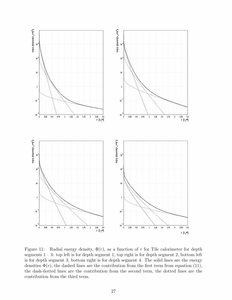
Using formula (11) and the values of the parameters ai, λi, given in Table 1, we havedetermined the underlying radial hadronic shower energy density functions, Φ(r). The resultsare shown in Figure 11 for depth segments 1 – 4 and in Figure 12 for the entire calorimeter.The contributions of the three terms of Φ(r) are also shown.

The functions Φ(r) for separate depth segments of a calorimeter are given in this paper forthe first time. The function Φ(r) for the entire calorimeter was previously given for a Lead-scintillating fiber calorimeter [16]; it is given here for the first time for an Iron-scintillatorcalorimeter. The analytical functions giving the radial energy density for different depthsegments allow to easily obtain the shower energy deposition in any calorimeter cell, showercontainment fractions and the cylinder radii for any given shower containment fraction.

The function Φ(r) for the entire calorimeter has been compared with the one for the lead-scintillating fiber calorimeter of ref. [16], that has about the same effective nuclear interactionlength for pions (namely 251 mm for the tile and 244 mm for the fiber calorimeter [20]).The two radial density functions are rather similar as seen in Fig. 13. The lead-scintillatingfiber calorimeter density function Φ(r), which was obtained from a 80 GeV π− grid scan atan angle of 2◦ with respect to the fiber direction, was parametrized using formula (6) withb1 = 0.169 pC/mm, b2 = 0.677 pC/mm, µ1 = 140 mm and µ2 = 42.4 mm. For the sake ofcomparing the radial density functions of the two calorimeters, the distribution from [16] wasnormalised to the Φ(r) of the Tile calorimeter. Precise agreement between these functionsshould not be expected because of the effect of the different absorber materials used in the

8

two detectors (e. g. the radiation/interaction length ratio for the Tile calorimeter is threetimes larger than for lead-scintillating fiber calorimeter [20]), the values of e/h are different,as is hadronic activity of showers because fewer neutrons are produced in iron than in lead[24], [25]).

6 Radial Containment

An other issue on which new results are presented here is the longitudinal development ofshower transverse dimensions. The parametrization of the radial density function, Φ(r),was integrated to yield the shower containment as a function of the radius, I(r). Figure 14shows the transverse containment of the pion shower, I(r), as a function of r for four depthsegments and for the entire calorimeter.

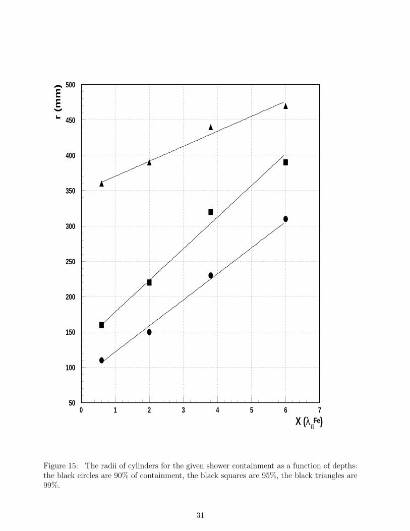
In Table 3 and Fig. 15 the radii of cylinders for the given shower containment (90%,95% and 99%) extracted from Fig. 14 as a function of depth are shown. The centers ofdepth segments, x, are given in units of λFe

π . Solid lines are the linear fits to the data:r(90%) = (85±6)+(37±3)x, r(95%) = (134±9)+(45±3)x, r(99%) = (349±7)+(22±2)x(mm). As can be seen, these containment radii increase linearly with depth. Such a linearincrease of 95% lateral shower containment with depth is also observed in an other iron-scintillator calorimeter at 50 and 140 GeV [26]. It is interesting to note that the showerradius for 95% radial containment for the entire calorimeter is equal to λeff

π = 251 mm [20]which justifies the frequently encountered statement that r(95%) ≈ λI [24], where λI is λ

effπ

in our case. For the entire Tile calorimeter the 99% containment radius is equal to 1.7± 0.1λeffπ .Based on our study, we believe that it is a poor approximation to regard the values ob-

tained from the marginal density function or the energy depositions in strips as the measureof the transverse shower containment, as was done in [4]. In that paper the value of 1.1 λeff

π

was obtained for 99% containment at 100 GeV, and the conclusion was drawn that their“result is consistent with the rule of thumb that a shower is contained within a cylinder ofradius equal to the interaction length of a calorimeter material”. However Tile calorimetermeasurements show that the cylinder radius for 99% shower containment is about two in-teraction lengths. If we extract the lateral shower containment dimension using instead theintegrated function F (z), given in Fig. 10, we obtain the value of 300 mm or 1.2 λeff

π , whichagrees with [4].

7 Longitudinal Profile

We have examined the differential deposition of energy ∆E/∆x as a function of x, thedistance along the shower axis. Table 4 lists the centers in x of the depth segments, x,and the lengths along x of the depth segments, ∆x, in units of λFe

π , the average showerenergy depositions in various depth segments, E0, and the energy depositions per interactionlength λFe

π , ∆E/∆x. Note that the values of E0 have been obtained taking into account thelongitudinal energy leakage which amounts to 1.8 GeV for 100 GeV [14].

Our values of ∆E/∆x together with the data of [27] and Monte Carlo predictions(GEANT-FLUKA + MICAP) [28] are shown in Fig. 16. The longitudinal energy depo-sition for our calorimeter using longitudinal orientation of the scintillating tiles is in goodagreement with that of a conventional iron-scintillator calorimeter.

The longitudinal profile, ∆E/∆x, may be approximated using two parametrizations. The

9

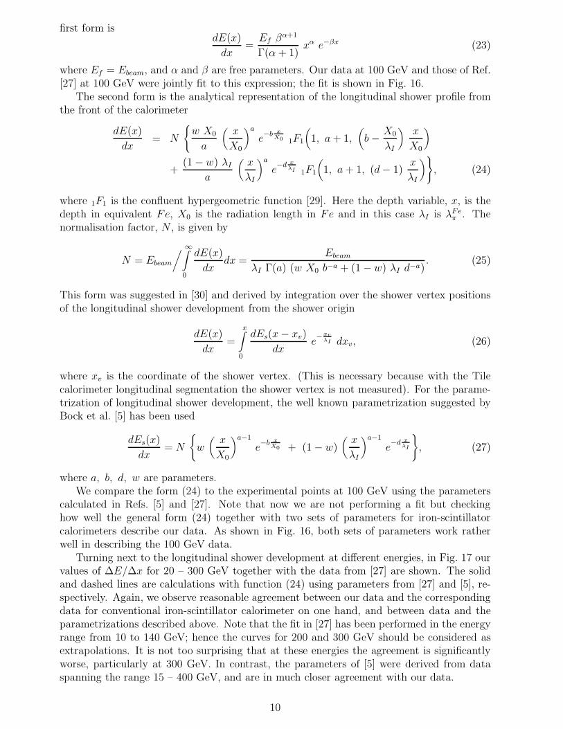
first form isdE(x)

dx=

Ef βα+1

Γ(α + 1)xα e−βx (23)

where Ef = Ebeam, and α and β are free parameters. Our data at 100 GeV and those of Ref.[27] at 100 GeV were jointly fit to this expression; the fit is shown in Fig. 16.

The second form is the analytical representation of the longitudinal shower profile fromthe front of the calorimeter

dE(x)

dx= N

{

w X0

a

(

x

X0

)a

e−b x

X0 1F1

(

1, a+ 1,(

b− X0

λI

)

x

X0

)

+(1− w) λI

a

(

x

λI

)a

e−d x

λI 1F1

(

1, a + 1, (d− 1)x

λI

)

}

, (24)

where 1F1 is the confluent hypergeometric function [29]. Here the depth variable, x, is thedepth in equivalent Fe, X0 is the radiation length in Fe and in this case λI is λFe

π . Thenormalisation factor, N , is given by

N = Ebeam

/

∞∫

0

dE(x)

dxdx =

Ebeam

λI Γ(a) (w X0 b−a + (1− w) λI d−a). (25)

This form was suggested in [30] and derived by integration over the shower vertex positionsof the longitudinal shower development from the shower origin

dE(x)

dx=

x∫

0

dEs(x− xv)

dxe−xv

λI dxv, (26)

where xv is the coordinate of the shower vertex. (This is necessary because with the Tilecalorimeter longitudinal segmentation the shower vertex is not measured). For the parame-trization of longitudinal shower development, the well known parametrization suggested byBock et al. [5] has been used

dEs(x)

dx= N

{

w(

x

X0

)a−1

e−b x

X0 + (1− w)(

x

λI

)a−1

e−d x

λI

}

, (27)

where a, b, d, w are parameters.We compare the form (24) to the experimental points at 100 GeV using the parameters

calculated in Refs. [5] and [27]. Note that now we are not performing a fit but checkinghow well the general form (24) together with two sets of parameters for iron-scintillatorcalorimeters describe our data. As shown in Fig. 16, both sets of parameters work ratherwell in describing the 100 GeV data.

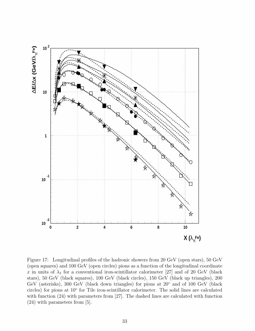
Turning next to the longitudinal shower development at different energies, in Fig. 17 ourvalues of ∆E/∆x for 20 – 300 GeV together with the data from [27] are shown. The solidand dashed lines are calculations with function (24) using parameters from [27] and [5], re-spectively. Again, we observe reasonable agreement between our data and the correspondingdata for conventional iron-scintillator calorimeter on one hand, and between data and theparametrizations described above. Note that the fit in [27] has been performed in the energyrange from 10 to 140 GeV; hence the curves for 200 and 300 GeV should be considered asextrapolations. It is not too surprising that at these energies the agreement is significantlyworse, particularly at 300 GeV. In contrast, the parameters of [5] were derived from dataspanning the range 15 – 400 GeV, and are in much closer agreement with our data.

10

8 The parametrization of Hadronic Showers

The three-dimensional parametrization for spatial hadronic shower development is

Ψ(x, r) =dE(x)

dx·

3∑

i=1

ai(x)λi(x)

K0(r

λi(x))

2π3∑

i=1ai(x)λi(x)

, (28)

where dE(x)/dx, defined by equation (24), is the longitudinal energy deposition, the func-tions ai(x) and λi(x) are given by equations (19) and (20), and K0 is the modified Besselfunction.

This explicit three dimensional parametrization can be used as a convenient tool for manycalorimetry problems requiring the integration of a shower energy deposition in a volumeand the reconstruction of the shower coordinates.

9 Electromagnetic Fraction of Hadronic Showers

One of the important issues in the understanding of hadronic showers is the electromagneticcomponent of the shower, i. e. the fraction of energy going into π0 production and its depen-dence on radial and longitudinal coordinates, fπ0(r, x). Following [16], we assume that theelectromagnetic part of a hadronic shower is the prominent central core, which in our case isthe first term in the expression (11) for the radial energy density function, Φ(r). Integratingfπ0 over r we get

fπ0 =a1λ1

3∑

i=1aiλi

. (29)

For the entire Tile calorimeter this value is (53± 3)% at 100 GeV.The observed π0 fraction, fπ0 , is related to the intrinsic actual fraction, f ′

π0 , by theequation

fπ0(E) =e E ′

em

e E ′em + h E ′

h

=e/h · f ′

π0(E)

(e/h− 1) · f ′π0(E) + 1

, (30)

where E ′em and E ′

h are the intrinsic electromagnetic and hadronic parts of shower energy,e and h are the coefficients of conversion of intrinsic electromagnetic and hadronic energiesinto observable signals, f ′

π0 = E ′em/(E

′em + E ′

h).There are two analytic forms for the intrinsic π0 fraction suggested by Groom [31]

f ′π0(E) = 1−

(

E

E ′0

)m−1

(31)

and Wigmans [32]

f ′π0(E) = k · ln

(

E

E ′0

)

, (32)

where E ′0 = 1 GeV, m = 0.85 and k = 0.11. We calculated fπ0 using the value e/h =

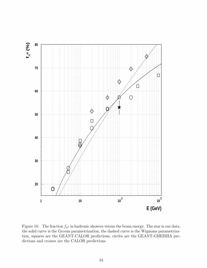
1.34± 0.03 for our calorimeter [2], [33] and obtained the curves shown in Fig. 18.Our result at 100 GeV is compared in Fig. 18 to the modified Groom and Wigmans

parametrizations and to results from the Monte Carlo codes CALOR [25], GEANT-GEISHA[28] and GEANT-CALOR [34] (the latter code is an implementation of CALOR89 differingfrom GEANT-FLUKA only for hadronic interactions below 10 GeV). Note that the MonteCarlo calculations were performed for the intrinsic π0 fraction, f ′

π0(E), and therefore the

11

results were modified by us according to (30). As can be seen from Fig. 18, our calculatedvalue of fπ0 is about one standard deviation lower than two of the Monte Carlo results andthe Groom and Wigmans parametrizations.

Figure 19 shows the fractions fπ0(r) as a function of r. As can be seen, the fractionsfπ0(r) for the entire calorimeter and for depth segments 1 – 3 amount to about 90% as r → 0and decrease to about 1% as r → λeff

π . However for depth segment 4 the value of fπ0(r)amounts to only 50% as r → 0 and decreases slowly to about 10% as r → λeff

π .Figure 20 shows the values of fπ0(x) as a function of x, as well as the linear fit which

gives fπ0(x) = (75± 2)− (8.4± 0.4)x (%).Using the values of fπ0(x) and energy depositions for various depth segments, we obtained

the contributions from the electromagnetic and hadronic parts of hadronic showers in Fig.16. The curves represent a fit to the electromagnetic and hadronic components of the showerusing equation (23). Ef is set equal to fπ0Ebeam for the electromagnetic fraction and (1 −fπ0)Ebeam for the hadronic fraction. The electromagnetic component of a hadronic showerrise and decrease more rapidly than the hadronic one (αem = 1.4±0.1, αh = 1.1±0.1, βem =1.12±0.04, βh = 0.65±0.05). The shower maximum position (xmax = (α/β) λeff

π ) occurs ata shorter distance from the calorimeter front face (xem

max = 1.23 λeffπ , xh

max = 1.85 λeffπ ). At

depth segments greater than 4 λeffπ , the hadronic fraction of the shower begins to dominate.

This is natural since the energy of the secondary hadrons is too low to permit significantpion production.

10 Summary and Conclusions

We have investigated the lateral development of hadronic showers using 100 GeV pion beamdata at an incidence angle of Θ = 10◦ for impact points z in the range from −360 to 200mm and the longitudinal development of hadronic showers using 20 – 300 GeV pion beamsat an incidence angle of Θ = 20◦.

Some useful formulae for the investigation of lateral profiles have been derived using athree-exponential form of the marginal density function f(z).

We have obtained for four depth segments and for the entire calorimeter: energy deposi-tions in towers, E(z); cumulative functions, F (z); underlying radial energy densities, Φ(r);the contained fraction of a shower as a function of radius, I(r); the radii of cylinders for agiven shower containment fraction; the fractions of the electromagnetic and hadronic partsof a shower; differential longitudinal energy deposition ∆E/∆x; and a three-dimensionalhadronic shower parametrization.

We have compared our data with those from a conventional iron-scintillator calorimeter,those from a lead-scintillator fiber calorimeter, and with Monte Carlo calculations. We havefound that there is general reasonable agreement in the behaviour of the Tile calorimeterradial density functions and those of the lead-scintillating fiber calorimeter; that the longi-tudinal profile agrees with that of a conventional iron-scintillator calorimeter and the MonteCarlo predictions; that the value at 100 GeV of the calculated fraction of energy going into π0

production in a hadronic shower, fπ0 , agrees with the Groom and Wigmans parametrizationsand with some of the Monte Carlo predictions.

The three-dimensional parametrization of hadronic showers that we obtained allows directuse in any application that requires volume integration of shower energy depositions andposition reconstruction. The experimental data on the transverse and longitudinal profiles,the radial energy densities and the three-dimensional hadronic shower parametrization areuseful for understanding the performance of the Tile calorimeter, but might find broaderapplication in Monte Carlo modeling of hadronic showers, in particular in fast simulations,

12

and for future calorimeter design.

11 Acknowledgements

This paper is the result of the efforts of many people from the ATLAS Collaboration. Theauthors are greatly indebted to the entire Collaboration for their test beam setup and datataking. We are grateful to the staff of the SPS, and in particular to Konrad Elsener, for theexcellent beam conditions and assistance provided during our tests.

References

[1] ATLAS Collaboration, ATLAS Technical Proposal for a General-Purpose pp Experi-ment at the Large Hadron Collider, CERN/LHCC/94-93, CERN, Geneva, Switzerland,1994.

[2] ATLAS Collaboration, ATLAS Tile Calorimeter Technical Design Report, ATLAS TDR3, CERN/LHCC/96-42, CERN, Geneva, Switzerland, 1996.

[3] R.K. Bock and A. Vasilescu, The Particle Detector Briefbook, Springer, 1998.

[4] W.J. Womersley et al., NIM A267 (1988) 49.

[5] R.K. Bock et al., NIM 186 (1981) 533.

[6] G. Grindhammer et al., NIM A289 (1990) 469.

[7] R. Brun et al., Proceedings of the Second Int. Conf. on Calorimetry in HEP, p. 82,Capri, Italy, 1991.

[8] E. Berger et al., CERN/LHCC 95-44, CERN, Geneva, Switzerland, 1995.

[9] M. Lokajicek et al., ATLAS Internal Note1, TILECAL-No-64, CERN, Geneva, Switzer-land, 1995.

[10] F. Ariztizabal et al., NIM A349 (1994) 384.

[11] M. Lokajicek et al., ATLAS Internal Note, TILECAL-No-63, CERN, Geneva, Switzer-land, 1995.

[12] I. Efthymiopoulos, A. Solodkov, The TILECAL Program for Test Beam Data Analysis,ATLAS Internal Note, TILECAL-No-101, CERN, Geneva, Switzerland, 1996.

[13] Application Software Group, PAW — Physics Analysis Workstation, CERN ProgramLibrary, entry Q121, CERN, Geneva, Switzerland, 1995.

[14] J.A. Budagov, Y.A. Kulchitsky, V.B. Vinogradov et al., JINR, E1-96-180, Dubna, Rus-sia, 1996; ATLAS Internal note, TILECAL-No-76, CERN, Geneva, Switzerland, 1996.

[15] R.M. Barnett et al., Review of Particle Physics, Probability, Phys. Rev. D54 (1996).

[16] D. Acosta et al., NIM A316 (1992) 184.

1 An Internet version of ATLAS Tile calorimeter Internal notes in postscript format are available at URLhttp://atlasinfo.cern.ch/Atlas/SUB DETECTORS/TILE/tileref/tinotes.html

13

[17] A.A. Lednev et al., NIM A366 (1995) 292.

[18] G.A. Akopdijanov et al., NIM 140 (1977) 441.

[19] E.T. Whitteker, G.N. Watson, A Course of Modern Analysis, Cambrige, Univ. Press,1927.

[20] J.A. Budagov, Y.A. Kulchitsky, V.B. Vinogradov et al., JINR, E1-97-318, Dubna, Rus-sia, 1997; ATLAS Internal note, TILECAL-No-127, CERN, Geneva, Switzerland, 1997.

[21] O.P. Gavrishchuk et al., JINR, P1-91-554, Dubna, Russia, 1991.

[22] F. Binon et al., NIM A206 (1983) 373.

[23] F. Barreiro et al., NIM A292 (1990) 259.

[24] C.W. Fabjan and T. Ludlam, Calorimetry in High-Energy Physics, Ann. Rev. Nucl.Part. Sci. 32 (1982).

[25] T.A. Gabriel et al., NIM A338 (1994) 336.

[26] M. Holder et al., NIM 151 (1978) 69.

[27] E. Hughes, Proc. of the I Int. Conf. on Calor. in HEP, p. 525, FNAL, Batavia, 1990.

[28] A. Juste, ATLAS Internal note, TILECAL-No-69, CERN, Geneva, Switzerland, 1995.

[29] M. Abramovitz and I.A. Stegun (Eds.), Handbook of Mathematical Functions, NationalBureau of Standards, Applied Mathematics, N.Y., Columbia Univ. Press, 1964.

[30] Y.A. Kulchitsky, V.B. Vinogradov, NIM A413 (1998) 484.

[31] D. Groom, Proceedings of the Workshop on Calorimetry for the Supercollider, Tusca-loosa, Alabama, USA, 1990.

[32] R. Wigmans, NIM A265 (1988) 273.

[33] J.A. Budagov, Y.A. Kulchitsky, V.B. Vinogradov et al., JINR, E1-95-513, Dubna, Rus-sia, 1995; ATLAS Internal note, TILECAL-No-72, CERN, Geneva, Switzerland, 1995.

[34] M. Bosman, Establishing Requiremements from the Point of View of the ATLAS Hadro-nic Barrel Calorimeter, ATLAS Workshop on Shower Models, 15 – 16 September 1997,CERN, Geneva, Switzerland, 1997.

14

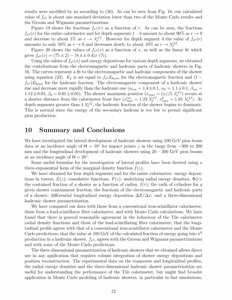
Table 1: The parameters ai and λi obtained by fitting the transverse shower profiles forfour depth segments and the entire calorimeter at 100 GeV.

Depth x (λFeπ ) a1 λ1 (mm) a2 λ2 (mm) a3 λ3 (mm)

1 0.6 0.88± 0.07 17± 2 0.12± 0.07 48± 14 0.004± 0.002 430± 2402 2.0 0.79± 0.06 25± 2 0.20± 0.06 52± 6 0.014± 0.006 220± 403 3.8 0.69± 0.03 32± 8 0.28± 0.03 71± 13 0.029± 0.005 280± 304 6.0 0.41± 0.05 51± 10 0.52± 0.06 73± 18 0.07± 0.03 380± 140

all four 0.78± 0.08 23± 1 0.20± 0.08 58± 4 0.015± 0.004 290± 40

Table 2: The values of the parameters αi, βi, γi and δi.

αi βi (1/λπ) γi (mm) δi (mm/λπ)

a1 0.99± 0.06 −0.088± 0.015 λ1 13± 2 6± 1a2 0.04± 0.06 0.071± 0.015 λ2 42± 10 6± 4a3 −0.001± 0.002 0.008± 0.002 λ3 170± 80 29± 23

15

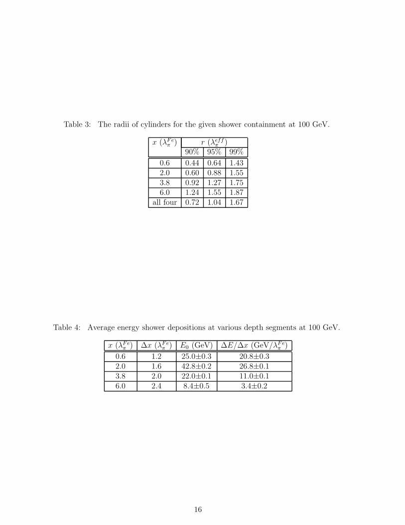
Table 3: The radii of cylinders for the given shower containment at 100 GeV.

x (λFeπ ) r (λeff

π )90% 95% 99%

0.6 0.44 0.64 1.432.0 0.60 0.88 1.553.8 0.92 1.27 1.756.0 1.24 1.55 1.87

all four 0.72 1.04 1.67

Table 4: Average energy shower depositions at various depth segments at 100 GeV.

x (λFeπ ) ∆x (λFe

π ) E0 (GeV) ∆E/∆x (GeV/λFeπ )

0.6 1.2 25.0±0.3 20.8±0.32.0 1.6 42.8±0.2 26.8±0.13.8 2.0 22.0±0.1 11.0±0.16.0 2.4 8.4±0.5 3.4±0.2

16

Doublereadout

Hadrons

Figure 1: Conceptual design of a Tile calorimeter module.

17

BC2 BC1

S2S3

S1

beam line

5 Module DetectorMuon wallNot to scale

Y Z

X

Figure 2: Schematic layout of the experimental setup. S1 – S3 are beam trigger scintillators,and BC1 – BC2 are (Z,Y) proportional chambers.

18

10-1

1

10

10 2

-600 -400 -200 0 200 400

Z (mm)

E(z

) (

GeV

)

10-1

1

10

10 2

-600 -400 -200 0 200 400

Z (mm)

E(z

) (

GeV

)

10-1

1

10

10 2

-600 -400 -200 0 200 400

Z (mm)

E(z

) (

GeV

)

10-1

1

10

10 2

-600 -400 -200 0 200 400

Z (mm)

E(z

) (

GeV

)

Figure 3: Energy depositions of 100 GeV pions in towers of depth segments 1 – 4 as afunction of the z coordinate: top left is for depth segment 1, top right is for depth segment2, bottom left is for depth segment 3, bottom right is for depth segment 4. Only statisticalerrors are shown. Curves are fits of equations (12) and (13) to the data.

19

1

10

10 2

-600 -400 -200 0 200 400

Z (mm)

E(z

) (

Ge

V)

Figure 4: Energy depositions in towers, summed over all calorimeter depth segments, as afunction of the z coordinate. Only statistical errors are shown. The curve is the result ofthe fit by formulas (12) and (13).

20

Figure 5: Schematic layout (top view) of Tile calorimeter experimental setup. z1 – z4 arethe distances between the centre of towers (for the four depth segments) and the directionof the beam particle.

21

10-2

10-1

1

0 100 200 300 400 500 600

Z (mm)

E(z

)/h

(G

eV

/ m

m)

Figure 6: The calculated marginal density function f(z) (the solid line) and the energy depo-sition function, E(z)/h, for various transverse sizes of a tower (h) : 50 mm (the dash-dottedline), 200 mm (the dashed line), 300 mm (the thick dotted line), 800 mm (the thin dottedline). The parameters for the entire calorimeter (see Table 1) are used in the calculations.

22

0

0.2

0.4

0.6

0.8

1

0 1 2 3 4 5 6 7

X (λπFe)

ai

Figure 7: X dependences of the parameters ai: the triangles are the a1 parameter, thediamonds are the a2, the squares are the a3.

23

0

10

20

30

40

50

60

0 1 2 3 4 5 6 7

X (λπFe)

λi (m

m)

Figure 8: X dependences of the parameters λi: the triangles are the λ1 parameter, thediamonds are the λ2, the squares are the λ3.

24

10-2

10-1

1

10

-400 -300 -200 -100 0 100 200 300 400

Z (mm)

F(z

) (G

eV

)

10-2

10-1

1

10

-400 -300 -200 -100 0 100 200 300 400

Z (mm)

F(z

) (

GeV

)

10-2

10-1

1

10

-400 -300 -200 -100 0 100 200 300 400

Z (mm)

F(z

) (

GeV

)

10-2

10-1

1

10

-400 -300 -200 -100 0 100 200 300 400

Z (mm)

F(z

) (

GeV

)

Figure 9: Cumulative functions F (z) for depth segments 1 – 4 as a function of the zcoordinate: top left is for depth segment 1, top right is for depth segment 2, bottom left isfor depth segment 3, bottom right is for depth segment 4. Statistical and systematic errors,summed in quadrature, are shown. Curves are fits of equations (16) and (17) to the data.

25

10-1

1

10

10 2

-400 -200 0 200 400

Z (mm)

F(z

) (G

eV

)

Figure 10: The cumulative function F (z) for the entire calorimeter as a function of the zcoordinate. Only statistical errors are shown. Curves are fits of equations (16) and (17) tothe data.

26

10-2

10-1

1

10

10 2

10 3

0 0.25 0.5 0.75 1 1.25 1.5 1.75 2 2.25 2.5

r (λπeff)

Φ(r

) (G

eV

/(λ

πeff)2

)

10-2

10-1

1

10

10 2

10 3

0 0.25 0.5 0.75 1 1.25 1.5 1.75 2 2.25 2.5

r (λπeff)

Φ(r

) (G

eV

/(λ

πeff)2

)

10-2

10-1

1

10

10 2

10 3

0 0.25 0.5 0.75 1 1.25 1.5 1.75 2 2.25 2.5

r (λπeff)

Φ(r

) (G

eV

/(λ

πeff)2

)

10-2

10-1

1

10

10 2

10 3

0 0.25 0.5 0.75 1 1.25 1.5 1.75 2 2.25 2.5

r (λπeff)

Φ(r

) (G

eV

/(λ

πeff)2

)

Figure 11: Radial energy density, Φ(r), as a function of r for Tile calorimeter for depthsegments 1 – 4: top left is for depth segment 1, top right is for depth segment 2, bottom leftis for depth segment 3, bottom right is for depth segment 4. The solid lines are the energydensities Φ(r), the dashed lines are the contribution from the first term from equation (11),the dash-dotted lines are the contribution from the second term, the dotted lines are thecontribution from the third term.

27

10-2

10-1

1

10

10 2

10 3

0 0.25 0.5 0.75 1 1.25 1.5 1.75 2 2.25 2.5

r (λπeff)

Φ(r

) (G

eV

/(λ

πe

ff)2

)

Figure 12: The radial energy density as a function of r (in units of λeffπ ) for Tile calorimeter

(the solid line), the contribution to Φ(r) from the first term in equation (11) (the dashedline), the contribution to Φ(r) from the second term (the dash-dotted line), the contributionto Φ(r) from the third term (the dotted line).

28

10-1

1

10

10 2

10 3

10 4

0 0.2 0.4 0.6 0.8 1 1.2 1.4 1.6 1.8 2

r (λπeff)

Φ(r

) (G

eV

/(λ

πe

ff)2

)

Figure 13: Comparison of the radial energy densities as a function of r (in units of λeffπ )

for Tile calorimeter (the solid line) and lead-scintillating fiber calorimeter (the dash-dottedline).

29

0

20

40

60

80

100

0 50 100 150 200 250 300 350 400 450 500

r (mm)

I (r

) (G

eV

)

Figure 14: Containment of shower I(r) (the solid line) as a function of radius for the entireTile calorimeter. The dash-dotted line is the contribution from the first depth segment, thedashed line is the contribution from the second depth segment, the thin dotted line is thecontribution from the third depth segment, the thick dotted line is the contribution fromthe fourth depth segment.

30

50

100

150

200

250

300

350

400

450

500

0 1 2 3 4 5 6 7

X (λπFe)

r (m

m)

Figure 15: The radii of cylinders for the given shower containment as a function of depths:the black circles are 90% of containment, the black squares are 95%, the black triangles are99%.

31

1

10

0 2 4 6 8 10

X (λπFe)

∆E

/∆x (

GeV

/λπF

e)

Figure 16: The longitudinal profile (circles) of the hadronic shower at 100 GeV as a functionof the longitudinal coordinate x in units of λFe

π . Open triangles are data from the calorimeterof Ref. [27], diamonds are the Monte Carlo (GEANT-FLUKA) predictions. The dash-dottedline is the fit by function (23), the solid line is calculated with function (24) with parametersfrom Ref. [27], the dashed line is calculated with function (24) with parameters from Ref. [5].The electromagnetic and hadronic components of the shower (crosses and squares), togetherwith their fits using (23), are discussed in Section 9.

32

10-2

10-1

1

10

10 2

0 2 4 6 8 10

X (λπFe)

∆E

/∆x (

GeV

/λπF

e)

Figure 17: Longitudinal profiles of the hadronic showers from 20 GeV (open stars), 50 GeV(open squares) and 100 GeV (open circles) pions as a function of the longitudinal coordinatex in units of λI for a conventional iron-scintillator calorimeter [27] and of 20 GeV (blackstars), 50 GeV (black squares), 100 GeV (black circles), 150 GeV (black up triangles), 200GeV (asterisks), 300 GeV (black down triangles) for pions at 20◦ and of 100 GeV (blackcircles) for pions at 10◦ for Tile iron-scintillator calorimeter. The solid lines are calculatedwith function (24) with parameters from [27]. The dashed lines are calculated with function(24) with parameters from [5].

33

20

30

40

50

60

70

80

1 10 102

103

E (GeV)

f πo (

%)

Figure 18: The fraction fπ0 in hadronic showers versus the beam energy. The star is our data,the solid curve is the Groom parametrization, the dashed curve is the Wigmans parametriza-tion, squares are the GEANT-CALOR predictions, circles are the GEANT-GHEISHA pre-dictions and crosses are the CALOR predictions.

34

10

20

30

40

50

60

70

80

90

100

0 0.1 0.2 0.3 0.4 0.5 0.6 0.7 0.8 0.9 1

r (λπeff)

f πo(r

) (

%)

Figure 19: The fπ0 fractions of hadronic showers as a function of radius. The solid lineis the fπ0(r) for the entire Tile calorimeter. The dash-dotted line is the fπ0(r) for the firstdepth segment, the dashed line is the fπ0(r) for the second depth segment, the thin dottedline is the fπ0(r) for the third depth segment, the thick dotted line is the fπ0(r) for the fourthdepth segment.

35

20

30

40

50

60

70

0 1 2 3 4 5 6 7

X (λπFe)

f πo(x

) (

%)

Figure 20: The fπ0(x) fractions of hadronic showers as a function of x.

36