HADES - Haskins Laboratories · sound systems, which can be ... HADES , called MHADES , ... each...

HADES(Haskins Analysis Display and Experiment System)

Philip Rubin, Ph.D.Vice President for Technical Resources

Research Staffemail: [email protected]

and

Anders Löfqvist, Ph.D.Research Staff

email: [email protected]

Haskins Laboratories, 270 Crown St.New Haven, CT 06511

www: http://www.haskins.yale.edu/

and

Yale University School of MedicineDepartment of Surgery (Otolaryngology)

I. INTRODUCTION

HADES (Haskins Analysis Display and Experiment System) refers to a family ofcomputer programs that has been developed at Haskins Laboratories to provide for the displayand analysis of multiple channel physiological, speech, and other sampled data in anexperimental context. HADES has become the main system for signal display and analysis atHaskins and is also being used at a number of academic research sites around the world(examples include Alfonso et al, 1993; Remez et al, 1994; Vatikiotis-Bateson et al, 1993,Vatikiotis-Bateson & Kelso, 1993, and Wada et al, in press). In general, HADES is used in twoways. The principal use of the system is for the display and analysis of physiological signals.These signals can be acquired from a variety of sources, including the optoelectronic positionmeasurement systems, the EMMA magnetometer hardware, and other transduction devices. Thesecond main use of HADES is for automated editing, labelling, and analysis of speech signals.This paper provides an overview of the HADES system, including a brief history of itsdevelopment, with the main intent of describing the features that are unique to this custom-developed signal processing system. Descriptions and figures are provided to show the mainfeatures of the system along with details about some of its more novel aspects. HADESincorporates a procedural programming language (SPIEL). A considerable portion of this paperwill describe this language and will include selected detailed programming examples.

Three main functions lie at the heart of the HADES system: display, manipulation andanalysis of sampled data. Signal vectors are separated from display tools to allow for multipleviews of the same data set. Data sets of up to 64 channels, supporting mixed sampling rates, canbe handled. A variety of display and analysis tools are available to the user. Some of these toolsare fairly general for the types of signals being used. Examples of standard displays includesimple time waveform plots, spectrograms, spectral cross-sections, etc. For analysis, we providestandard Discrete Fourier Transform (DFT) and Linear Predictive Coding (LPC) analyses. Othertools are more specific to the research environment at Haskins Laboratories and have been (orare being) developed in the context of these needs. In particular, the evolution of HADES hasbeen strongly influenced by the use of an electromagnetic midsagittal articulometer (EMMA) foracquiring information about speech production (Perkell, Cohen, Svirsky, Matthies, Garabieta,and Jackson, 1992; Gracco and Nye, 1993). We have found, however, that most of the tools andprimitives that we have developed are of use to researchers outside of Haskins Laboratories. Lessstandard displays and analyses include phase and lissajous plots, TIFF displays, animation ofvocal tract articulator markers, centroid calculations, event marking, etc.

The most significant feature of HADES is the incorporation of a procedural language(known as SPIEL, Signal Processing Interactive Editing Language). SPIEL permits the creationand customization of specialized analysis procedures that can be stored as text files, edited, etc.,and are similar to functions and subroutines in programming languages like C and Fortran.SPIEL procedures are either interpreted from command-line entry or from text stored in ASCIIcommand files. Signals (which are vectors of time-varying numerical values) are treated asprimitives and can be manipulated (added, multiplied, etc.) as if they were numerical variables.All of the program’s options are also available to the language as variables, and most operationsof the programs can be specified as commands. This procedural language lets users automateroutine operations, such as labelling and removing stretches of silence, and permits simpleprocessing/analysis, within individual signals and across sets of separate signals.

The HADES system was designed to run on VAX computers, using the VMS operatingsystem. The program is written in C, however some of the signal processing routines,particularly those based on the IEEE package of digital signal processing routines (IEEE, 1979),were written in Fortran. The development of HADES on a VAX platform combines historical

Rubin and Löfqvist, HADES 2

configuration requirements at Haskins Laboratories (described below) along with the need for ananalysis package that would run on engineering workstations. In a limited form (text only), theprogram will run on any terminal connected to a VAX and can also be accessed via Ethernetfrom microcomputer terminals that support either Tektronix 4010/4014 graphics or XWindows/Motif emulation. Audio input and output is done using networked Gradient DeskLabsound systems, which can be accessed from most of our VAX workstations.

A variety of flavors of HADES exist. These are related, again, to the historicaldevelopment of the system at Haskins Laboratories along with changing workstation graphicaluser interface (GUI) standards. At present, HADES exists in two main flavors: HADES, whichruns on VAX VMS workstations that support UIS graphics (Rubin, et al, 1991); and XHADES,which runs on VAX VMS workstations that support X Windows graphics. A third version ofHADES, called MHADES, is presently under development. MHADES is designed for fullcompatibility with the DECwindows Motif user interface. Finally, AHADES is in the planningstages. AHADES is a version of MHADES that will run on Digital’s newer Alpha (DEC AXP)platform. In general, we will refer to all members or the HADES family of programs by thegeneric HADES name.

II. HISTORY

A detailed description of the history of the development of the HADES is provided inRubin (1995). The exact character of the HADES system has been shaped by several majorinfluences. In brief, the main factors have been (a) the desire to modernize and consolidate avariety of existing signal-related programs at Haskins Laboratories; (b) the need to provide acustom software facility for handling the large data sets generated in experiments using theEMMA system at Haskins; and (c) the change to engineering workstations that used rastergraphics for display and provided tools for developing sophisticated graphical user interfaces.

During the 1970s a large set of signal processing programs was developed at HaskinsLaboratories. These programs were written for a Digital PDP-11/45 and then a VAX 11/780. Oneof the most important of these was WENDY (Szubowicz, 1982), a waveform editing program thatincluded a primitive procedural language for performing iterative operations and defining macrosto repeat complex or frequently used operations. WENDY ran on a single CPU that supported anumber of Tektronix 4010/4014 compatible storage display terminals. Shortly after thedevelopment of WENDY, a program called SPA (SPectral Analysis) was designed to provideDFT-based spectral analysis based on the IEEE package of signal processing subroutines (IEEE,1979). SPA was intended to supplement ILS (Interactive Laboratory System), a commercialpackage of LPC-based analysis and filtering routines from Signal Technology Incorporated. Awide variety of other related programs were being used at Haskins at this point in time includingprograms for supporting sampled data files such as AFM (Arithmetic File Manipulation), CPC(viewing PCM data), INPUT (converting analog signals to digital form), and OUTPUT (digital toanalog). The PSP (Physiological Signal Processing), ACT, and ACE programs were developed todisplay and analyze physiological time domain data.

Shortly after we began using one of our first engineering workstation (a VAXstationII/GPX), in 1986, development began on a prototype for a new display/analysis system. Severalmajor design considerations were at the heart this project, including:

• the development of a graphical user interface for ease of use (including multiple display windows, menus, dialog boxes, etc.)

• a command window for entering text commands and/or command strings


• multiple waveforms in multi-panel windows, for manipulation of multi-channel data (e.g. physiological measurement, dichotic speech)

• the consolidation of a variety of signal-processing functions from our other programs

• a rich set of signal-processing primitives, tailored to our particular needs

• specialized display primitives

• the implementation of a procedural programming language within the program.

Although microcomputer-based systems existed (see, for example, Jamieson, et al,1989), internal considerations dictated a VAXstation-based system. In particular this decisionwas influenced by the existence of a wide variety of other custom-developed VAX software thatwere using, and could not easily rewrite or replace. Our design decisions were also influenced bysome of the other workstation-based systems developed during this period. Examples includeSpire (Cyphers, 1985; Zue et al, 1986), MITSYN (Henke, 1987), and ESPIRIT (Gayvert, Biles,Rhody, and Hillenbrand, 1989). The result of this initial prototyping process was a programcalled SPEED (Maverick & Rubin, 1988). SPEED was a signal processing display and editingprogram that was implemented on a VAXstation II/GPX equipped with Data Translation D/Aand A/D boards, attached to the Q-Bus, for signal input and output.

SPEED was conceived as a prototype and was never intended to be a large-scale system.Our next step was the beginning of the development of an environment that included anextensible programming language with flexible signal processing primitives, and was also fullyintegrated with other Haskins software tools. The Haskins Analysis Display and ExperimentSystem (HADES) provided a vehicle for standardizing and consolidating many of the signalprocessing tools (e.g. SPA, PSP, ACT, ACE, AFM, etc.) that had been developed at theLaboratories over the years. At this point in time, the HADES design was also heavily influencedby our acquisition of an electromagnetic midsagittal articulometer (EMMA) system (Perkell etal, 1992).

Löfqvist, Gracco and Nye (1993) have pointed out that processing two-dimensionalmovement signals like those obtained from a magnetometer system often requires the handlingand storing of a large amount of data. They note:

“In a typical experiment, x and y position signals are obtained from which velocity andacceleration may be derived. In some systems, a correction index is also recorded foreach receiver coil, providing information on the operation of the tilt correctionalgorithm. If data from nine receivers have been recorded together with the audio signalduring the production of many utterances with several repetitions of each, the numberof data files tends to grow very quickly. Software is required for opening and displayingmultiple signal files, marking events such as the peaks, valleys and zero crossings insignals, and making measurements of the labeled signals. In addition to displayingposition or velocity over time, it is also very useful to display x-y position plots of signalsso that articulatory movement trajectories can be observed. Furthermore, it is helpful tohave routines for filtering, differentiating, and averaging of signals and to derive newrepresentations of the data using functions of the position information. Since many ofthe processing routines will be used repetitively on tokens and utterances, it saves timeto automate these routines as much as possible. At Haskins, we have developed asoftware package, Haskins Analysis Display and Experiment System (HADES), thatincorporates most of these features ... ”


Based on the design and potential use of the EMMA system, it was determined that thedevelopment of HADES would require a system that flexibly handled large numbers ofindependent channels of data. This resulted in certain fundamental constructs in HADES,including the signal primitive (a vector of numerical data, usually representing time-varyinginformation, which can be manipulated internally as if it were a variable in a programminglanguage), string manipulation routines for creating filenames, facilities for outputting data toboth binary and ASCII files, customized display primitives, analysis tools customized to our ownparticular experimental requirements, and an integrated language that would support the rapidcreation of procedures specific to our particular needs. The rest of this paper provides anoverview of HADES, along with detailed programming examples using the procedural language.

III. HADES FEATURES

III.A. HADES User Interface

III.A.1. The HADES Desktop

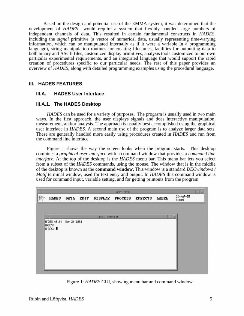
HADES can be used for a variety of purposes. The program is usually used in two mainways. In the first approach, the user displays signals and does interactive manipulation,measurement, and/or analysis. The approach is usually best accomplished using the graphicaluser interface in HADES. A second main use of the program is to analyze larger data sets.These are generally handled more easily using procedures created in HADES and run fromthe command line interface.

Figure 1 shows the way the screen looks when the program starts. This desktopcombines a graphical user interface with a command window that provides a command lineinterface. At the top of the desktop is the HADES menu bar. This menu bar lets you selectfrom a subset of the HADES commands, using the mouse. The window that is in the middleof the desktop is known as the command window. This window is a standard DECwindows /Motif terminal window, used for text entry and output. In HADES this command window isused for command input, variable setting, and for getting printouts from the program.

Figure 1: HADES GUI, showing menu bar and command window


Command line input consists of any valid HADES statement, which can be a command,or a line of text that can interpreted by the program, such as A=7. Details about HADEScommands are provided elsewhere in this document and a listing of selected commands canbe found in Appendix II. From the Command Window, variables can be set, includingnumbers and strings. In addition, flag variables can be set to selected constants. A listing ofHADES functions is provided in Appendix III. Shown below is a short transcript of a HADEScommand line session in which a sampled data file (COW.PCM) is opened, smoothed, andsaved with a new name (SCOW.PCM). Note that the HADES command line syntax is fairlystraightforward.

(Note: In the following example, text shown in bold has been printed on the screen by theprogram.)

HADES> open cowreading file MIKE$DUB0:[RUBIN.HADES]COW.PCM;1signal COW createdHADES> smooth cowHADES> save cow as scow COW SAVED AS SCOW.PCMHADES>

III.A.2. The Menu Bar

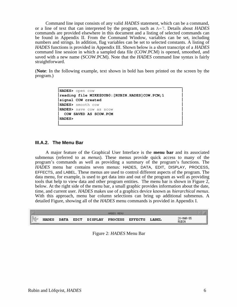
A major feature of the Graphical User Interface is the menu bar and its associatedsubmenus (referred to as menus). These menus provide quick access to many of theprogram’s commands as well as providing a summary of the program’s functions. TheHADES menu bar contains seven menus: HADES, DATA, EDIT, DISPLAY, PROCESS,EFFECTS, and LABEL. These menus are used to control different aspects of the program. Thedata menu, for example, is used to get data into and out of the program as well as providingtools that help to view data and other program entities. The menu bar is shown in Figure 2,below. At the right side of the menu bar, a small graphic provides information about the date,time, and current user. HADES makes use of a graphics device known as hierarchical menus.With this approach, menu bar column selections can bring up additional submenus. Adetailed Figure, showing all of the HADES menu commands is provided in Appendix I.

Figure 2: HADES Menu Bar


III.A.3. Dialog boxes

A standard component of most programs that include a graphical user interface is thedialog box. Dialog boxes provide a quick method for specifying command and programoptions, and for entering text and numerical information. This is often crucial for lessexperienced users of programs, particularly if the program has a wide range of possiblechoices. The dialog box can serve as self-documentation for a program by displaying therelevant variables, flags, and other potential selections. In addition, dialog boxes help toorganize options into functional groups and provide constraints that help to minimize usererror. HADES makes use of dialog boxes in a number of different areas. The Menu Barincludes commands, such as SPECTRAL ANALYSIS, or FILTER, that result in a dialog boxbeing presented. Most of the display windows in HADES (described below) include aToolbox icon that results in a dialog box being displayed. An example of the first type ofdialog box is shown in Figure 3. This is the Analysis Parameters Dialog Box used forcustomizing the spectral analysis parameters. The boxes on the top row are known as buttons.Clicking on any one of these will choose a set of analysis parameters (WINDOW TYPE,WINDOW SIZE and WINDOW SEPARATION) with one quick operation. The WINDOW TYPEbox shows another type of button — this is a pop-up menu button: a list of different optionsfor WINDOW TYPE will be shown with selection being done by clicking and dragging. TheWINDOW SEPARATION box allows for direct entry by typing a value into the box.Alternatively, clicking on the right and left arrows will step the value up or down. The threebuttons at the bottom of the box are more straightforward. Clicking on the CANCEL buttonwill exit the dialog, and return you to the state you were in prior to making changes to thevalues in the dialog box. Clicking on ACCEPT will change the specified variables, but take nofurther action. Clicking on the EXECUTE will change the specified variables and then analyzethe appropriate signal. Dialog boxes similar to this one are used throughout HADES. Thisexample describes only a portion of the types of data entry that are used in the program.

Figure 3: Analysis Parameters Dialog Box


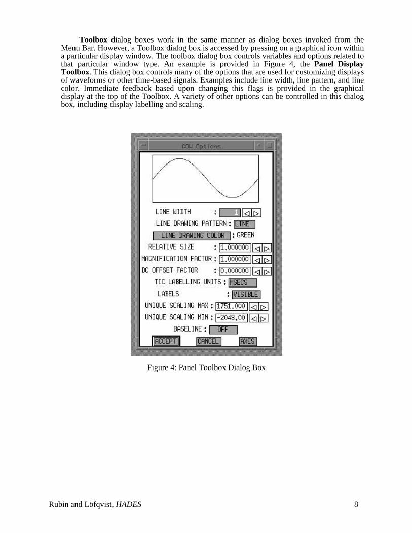
Toolbox dialog boxes work in the same manner as dialog boxes invoked from theMenu Bar. However, a Toolbox dialog box is accessed by pressing on a graphical icon withina particular display window. The toolbox dialog box controls variables and options related tothat particular window type. An example is provided in Figure 4, the Panel DisplayToolbox. This dialog box controls many of the options that are used for customizing displaysof waveforms or other time-based signals. Examples include line width, line pattern, and linecolor. Immediate feedback based upon changing this flags is provided in the graphicaldisplay at the top of the Toolbox. A variety of other options can be controlled in this dialogbox, including display labelling and scaling.

Figure 4: Panel Toolbox Dialog Box


III.A.4. Windows

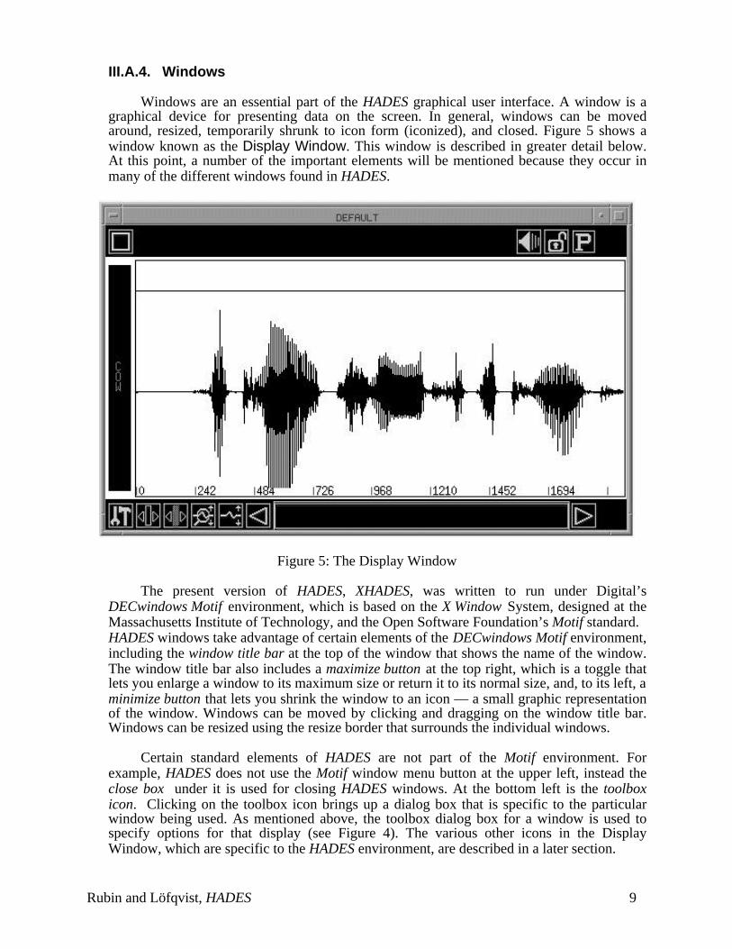
Windows are an essential part of the HADES graphical user interface. A window is agraphical device for presenting data on the screen. In general, windows can be movedaround, resized, temporarily shrunk to icon form (iconized), and closed. Figure 5 shows awindow known as the Display Window. This window is described in greater detail below.At this point, a number of the important elements will be mentioned because they occur inmany of the different windows found in HADES.

Figure 5: The Display Window

The present version of HADES, XHADES, was written to run under Digital’sDECwindows Motif environment, which is based on the X Window System, designed at theMassachusetts Institute of Technology, and the Open Software Foundation’s Motif standard.HADES windows take advantage of certain elements of the DECwindows Motif environment,including the window title bar at the top of the window that shows the name of the window.The window title bar also includes a maximize button at the top right, which is a toggle thatlets you enlarge a window to its maximum size or return it to its normal size, and, to its left, aminimize button that lets you shrink the window to an icon — a small graphic representationof the window. Windows can be moved by clicking and dragging on the window title bar.Windows can be resized using the resize border that surrounds the individual windows.

Certain standard elements of HADES are not part of the Motif environment. Forexample, HADES does not use the Motif window menu button at the upper left, instead theclose box under it is used for closing HADES windows. At the bottom left is the toolboxicon. Clicking on the toolbox icon brings up a dialog box that is specific to the particularwindow being used. As mentioned above, the toolbox dialog box for a window is used tospecify options for that display (see Figure 4). The various other icons in the DisplayWindow, which are specific to the HADES environment, are described in a later section.


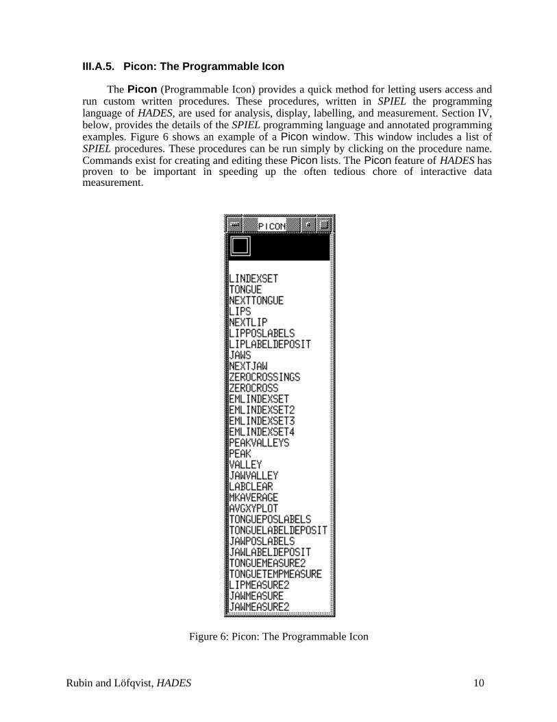
III.A.5. Picon: The Programmable Icon

The Picon (Programmable Icon) provides a quick method for letting users access andrun custom written procedures. These procedures, written in SPIEL the programminglanguage of HADES, are used for analysis, display, labelling, and measurement. Section IV,below, provides the details of the SPIEL programming language and annotated programmingexamples. Figure 6 shows an example of a Picon window. This window includes a list ofSPIEL procedures. These procedures can be run simply by clicking on the procedure name.Commands exist for creating and editing these Picon lists. The Picon feature of HADES hasproven to be important in speeding up the often tedious chore of interactive datameasurement.

Figure 6: Picon: The Programmable Icon


III.B. HADES Displays

Fundamental to the HADES environment is a rich set of graphical tools used torepresent, and allow the manipulation of, a variety of different data types. The focus of thesetools is on sampled data time-based signals, but also includes displays for spectralinformation and gray-scale images. This section provides an overview of the HADES displaytools.

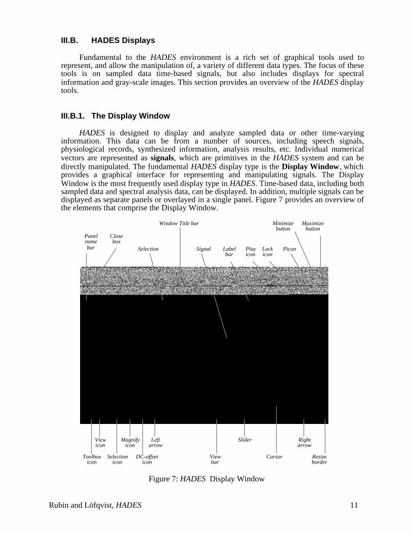
III.B.1. The Display Window

HADES is designed to display and analyze sampled data or other time-varyinginformation. This data can be from a number of sources, including speech signals,physiological records, synthesized information, analysis results, etc. Individual numericalvectors are represented as signals, which are primitives in the HADES system and can bedirectly manipulated. The fundamental HADES display type is the Display Window, whichprovides a graphical interface for representing and manipulating signals. The DisplayWindow is the most frequently used display type in HADES. Time-based data, including bothsampled data and spectral analysis data, can be displayed. In addition, multiple signals can bedisplayed as separate panels or overlayed in a single panel. Figure 7 provides an overview ofthe elements that comprise the Display Window.

Selection

Window Title bar Maximizebutton

Panelnamebar

Closebox

Signal Playicon

Minimizebutton

Labelbar

Lockicon

Picon

Viewicon

Magnifyicon

Leftarrow

Slider

Toolboxicon

Viewbar

Resizeborder

Rightarrow

CursorSelectionicon

DC-offseticon

Figure 7: HADES Display Window


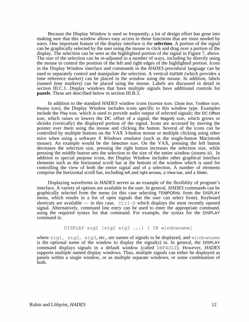
Because the Display Window is used so frequently, a lot of design effort has gone intomaking sure that this window allows easy access to those functions that are most needed byusers. One important feature of the display interface is the selection. A portion of the signalcan be graphically selected by the user using the mouse to click and drag over a portion of thedisplay. The selection can be seen as the highlighted portion of the signal in Figure 7, above.The size of the selection can be re-adjusted in a number of ways, including by directly usingthe mouse to control the position of the left and right edges of the highlighted portion. Iconsin the Display Window interface and commands in the HADES procedural language can beused to separately control and manipulate the selection. A vertical cursor (which provides atime reference marker) can be placed in the window using the mouse. In addition, labels(named time markers) can be placed using the mouse. Labels are discussed in detail insection III.C.1. Display windows that have multiple signals have additional controls forpanels. These are described below in section III.B.3.

In addition to the standard HADES window icons (Iconize Icon, Close box, Toolbox icon,Resize icon), the Display Window includes icons specific to this window type. Examplesinclude the Play icon, which is used to provide audio output of selected signals; the DC-Offseticon, which raises or lowers the DC offset of a signal; the Magnify icon, which grows orshrinks (vertically) the displayed portion of the signal. Icons are accessed by moving thepointer over them using the mouse and clicking the button. Several of the icons can becontrolled by multiple buttons on the VAX 3-button mouse or multiple clicking using othermice when using a software X Windows emulator (such as the single-button Macintoshmouse). An example would be the Selection icon. On the VAX, pressing the left buttondecreases the selection size, pressing the right button increases the selection size, whilepressing the middle button sets the selection to the size of the entire window (zooms it). Inaddition to special purpose icons, the Display Window includes other graphical interfaceelements such as the horizontal scroll bar at the bottom of the window which is used forcontrolling the view of both the entire signal and of a selection. A number of elementscomprise the horizontal scroll bar, including left and right arrows, a View bar, and a Slider.

Displaying waveforms in HADES serves as an example of the flexibility of program’sinterface. A variety of options are available to the user. In general, HADES commands can begraphically selected from the menu (in this case selecting TEMPORAL from the DISPLAYmenu, which results in a list of open signals that the user can select from). Keyboardshortcuts are available — in this case, Ctrl-D which displays the most recently openedsignal. Alternatively, command line entry can be used to enter the appropriate command,using the required syntax for that command. For example, the syntax for the DISPLAYcommand is:

DISPLAY sig1 [sig2 sig3 ...] [ IN windowname]

where sig1, sig2, sig3, etc., are names of signals to be displayed, and windownameis the optional name of the window to display the signal(s) in. In general, the DISPLAYcommand displays signals in a default window (called DEFAULT). However, HADESsupports multiple named display windows. Thus, multiple signals can either be displayed aspanels within a single window, or as multiple separate windows, or some combination ofboth.


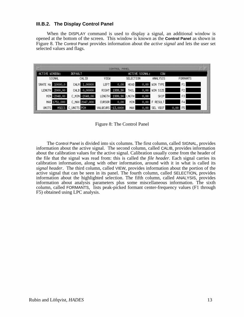
III.B.2. The Display Control Panel

When the DISPLAY command is used to display a signal, an additional window isopened at the bottom of the screen. This window is known as the Control Panel as shown inFigure 8. The Control Panel provides information about the active signal and lets the user setselected values and flags.

Figure 8: The Control Panel

The Control Panel is divided into six columns. The first column, called SIGNAL, providesinformation about the active signal. The second column, called CALIB, provides informationabout the calibration values for the active signal. Calibration usually come from the header ofthe file that the signal was read from: this is called the file header. Each signal carries itscalibration information, along with other information, around with it in what is called itssignal header. The third column, called VIEW, provides information about the portion of theactive signal that can be seen in its panel. The fourth column, called SELECTION, providesinformation about the highlighted selection. The fifth column, called ANALYSIS, providesinformation about analysis parameters plus some miscellaneous information. The sixthcolumn, called FORMANTS, lists peak-picked formant center-frequency values (F1 throughF5) obtained using LPC analysis.


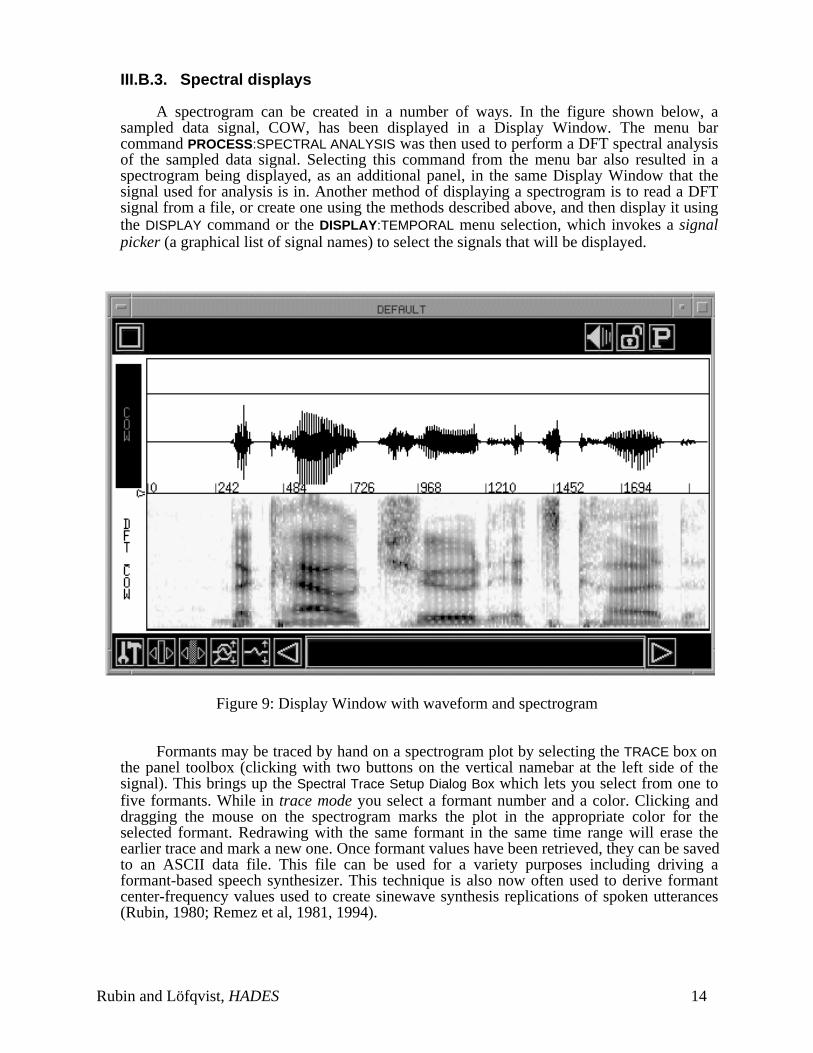
III.B.3. Spectral displays

A spectrogram can be created in a number of ways. In the figure shown below, asampled data signal, COW, has been displayed in a Display Window. The menu barcommand PROCESS:SPECTRAL ANALYSIS was then used to perform a DFT spectral analysisof the sampled data signal. Selecting this command from the menu bar also resulted in aspectrogram being displayed, as an additional panel, in the same Display Window that thesignal used for analysis is in. Another method of displaying a spectrogram is to read a DFTsignal from a file, or create one using the methods described above, and then display it usingthe DISPLAY command or the DISPLAY:TEMPORAL menu selection, which invokes a signalpicker (a graphical list of signal names) to select the signals that will be displayed.

Figure 9: Display Window with waveform and spectrogram

Formants may be traced by hand on a spectrogram plot by selecting the TRACE box onthe panel toolbox (clicking with two buttons on the vertical namebar at the left side of thesignal). This brings up the Spectral Trace Setup Dialog Box which lets you select from one tofive formants. While in trace mode you select a formant number and a color. Clicking anddragging the mouse on the spectrogram marks the plot in the appropriate color for theselected formant. Redrawing with the same formant in the same time range will erase theearlier trace and mark a new one. Once formant values have been retrieved, they can be savedto an ASCII data file. This file can be used for a variety purposes including driving aformant-based speech synthesizer. This technique is also now often used to derive formantcenter-frequency values used to create sinewave synthesis replications of spoken utterances(Rubin, 1980; Remez et al, 1981, 1994).


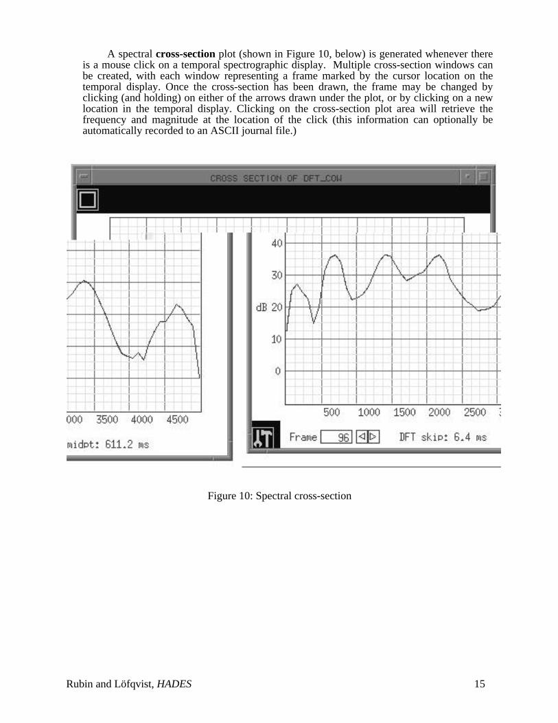
A spectral cross-section plot (shown in Figure 10, below) is generated whenever thereis a mouse click on a temporal spectrographic display. Multiple cross-section windows canbe created, with each window representing a frame marked by the cursor location on thetemporal display. Once the cross-section has been drawn, the frame may be changed byclicking (and holding) on either of the arrows drawn under the plot, or by clicking on a newlocation in the temporal display. Clicking on the cross-section plot area will retrieve thefrequency and magnitude at the location of the click (this information can optionally beautomatically recorded to an ASCII journal file.)

Figure 10: Spectral cross-section


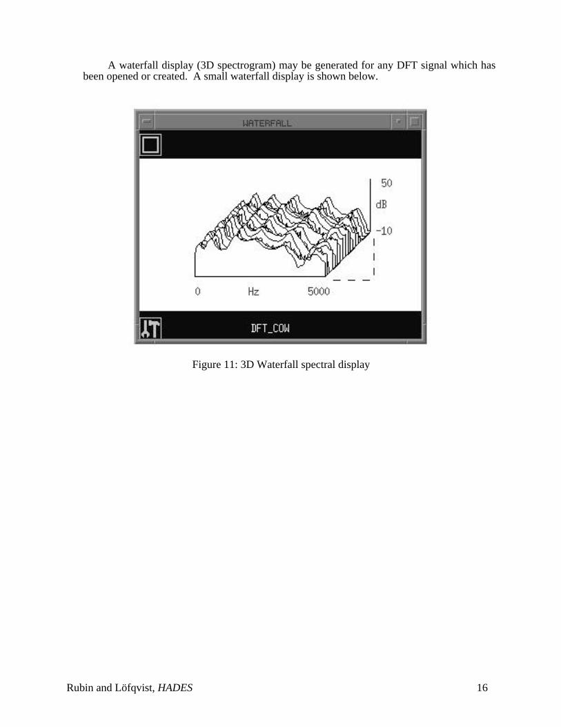
A waterfall display (3D spectrogram) may be generated for any DFT signal which hasbeen opened or created. A small waterfall display is shown below.

Figure 11: 3D Waterfall spectral display


III.B.4. Multiple Panel displays

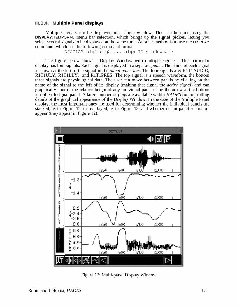
Multiple signals can be displayed in a single window. This can be done using theDISPLAY:TEMPORAL menu bar selection, which brings up the signal picker, letting youselect several signals to be displayed at the same time. Another method is to use the DISPLAYcommand, which has the following command format:

DISPLAY sig1 sig2 ... sign IN windowname

The figure below shows a Display Window with multiple signals. This particulardisplay has four signals. Each signal is displayed in a separate panel. The name of each signalis shown at the left of the signal in the panel name bar. The four signals are: R1T1AUDIO,R1T1ULY, R1T1LLY, and R1T1PRES. The top signal is a speech waveform, the bottomthree signals are physiological data. The user can move between panels by clicking on thename of the signal to the left of its display (making that signal the active signal) and cangraphically control the relative height of any individual panel using the arrow at the bottomleft of each signal panel. A large number of flags are available within HADES for controllingdetails of the graphical appearance of the Display Window. In the case of the Multiple Paneldisplay, the most important ones are used for determining whether the individual panels arestacked, as in Figure 12, or overlayed, as in Figure 13, and whether or not panel separatorsappear (they appear in Figure 12).

Figure 12: Multi-panel Display Window


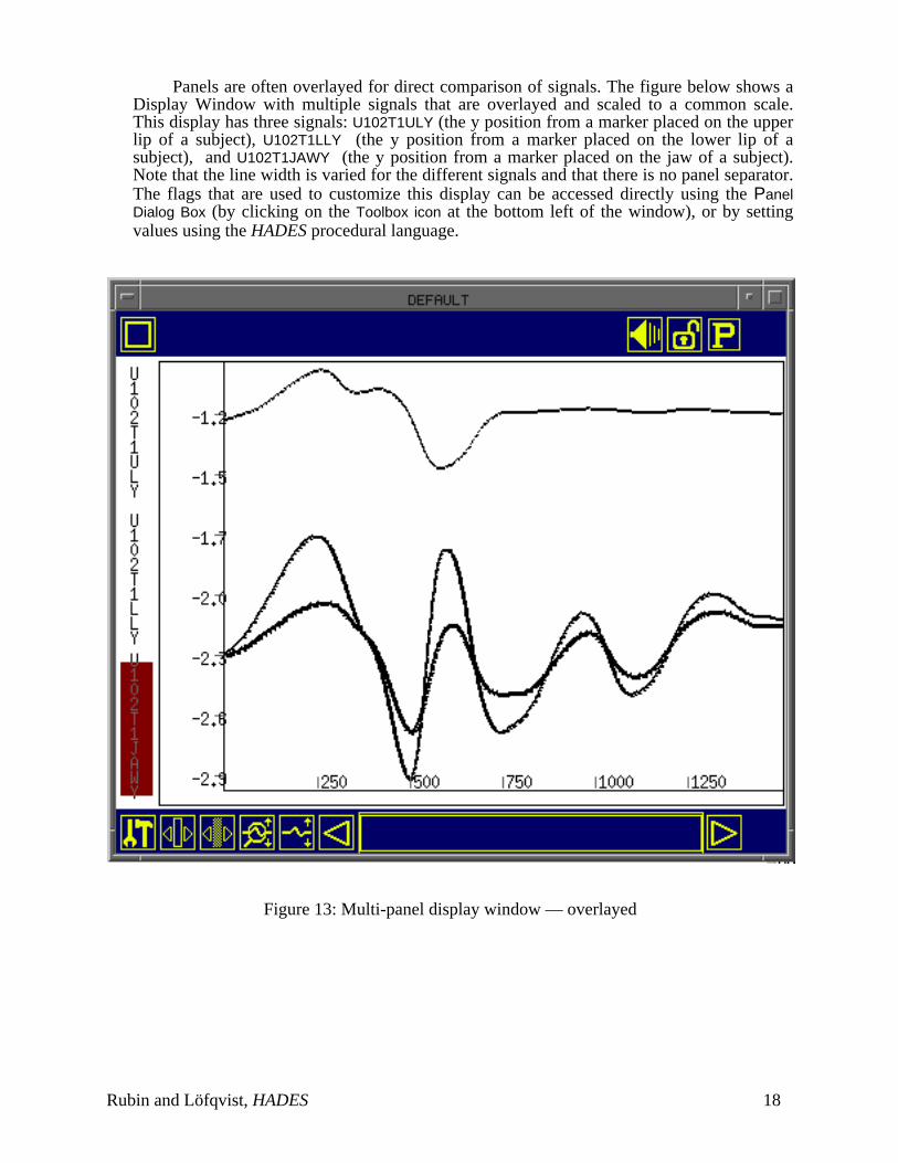
Panels are often overlayed for direct comparison of signals. The figure below shows aDisplay Window with multiple signals that are overlayed and scaled to a common scale.This display has three signals: U102T1ULY (the y position from a marker placed on the upperlip of a subject), U102T1LLY (the y position from a marker placed on the lower lip of asubject), and U102T1JAWY (the y position from a marker placed on the jaw of a subject).Note that the line width is varied for the different signals and that there is no panel separator.The flags that are used to customize this display can be accessed directly using the PanelDialog Box (by clicking on the Toolbox icon at the bottom left of the window), or by settingvalues using the HADES procedural language.

Figure 13: Multi-panel display window — overlayed


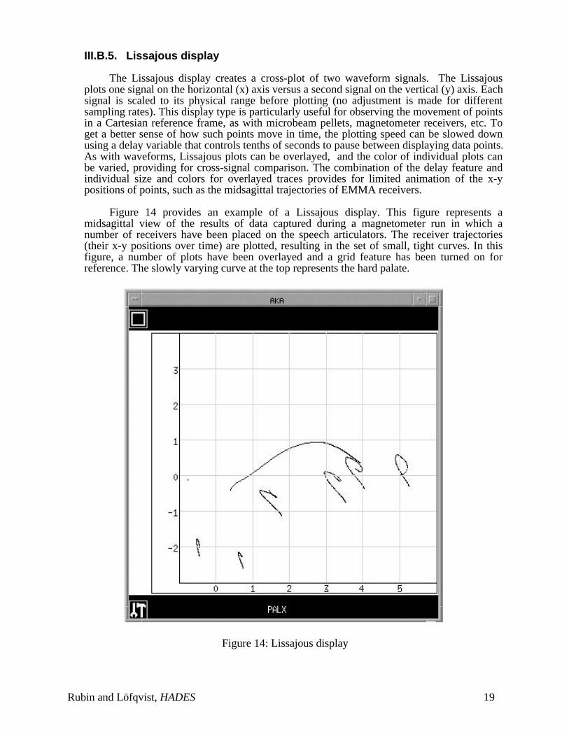
III.B.5. Lissajous display

The Lissajous display creates a cross-plot of two waveform signals. The Lissajousplots one signal on the horizontal (x) axis versus a second signal on the vertical (y) axis. Eachsignal is scaled to its physical range before plotting (no adjustment is made for differentsampling rates). This display type is particularly useful for observing the movement of pointsin a Cartesian reference frame, as with microbeam pellets, magnetometer receivers, etc. Toget a better sense of how such points move in time, the plotting speed can be slowed downusing a delay variable that controls tenths of seconds to pause between displaying data points.As with waveforms, Lissajous plots can be overlayed, and the color of individual plots canbe varied, providing for cross-signal comparison. The combination of the delay feature andindividual size and colors for overlayed traces provides for limited animation of the x-ypositions of points, such as the midsagittal trajectories of EMMA receivers.

Figure 14 provides an example of a Lissajous display. This figure represents amidsagittal view of the results of data captured during a magnetometer run in which anumber of receivers have been placed on the speech articulators. The receiver trajectories(their x-y positions over time) are plotted, resulting in the set of small, tight curves. In thisfigure, a number of plots have been overlayed and a grid feature has been turned on forreference. The slowly varying curve at the top represents the hard palate.

Figure 14: Lissajous display


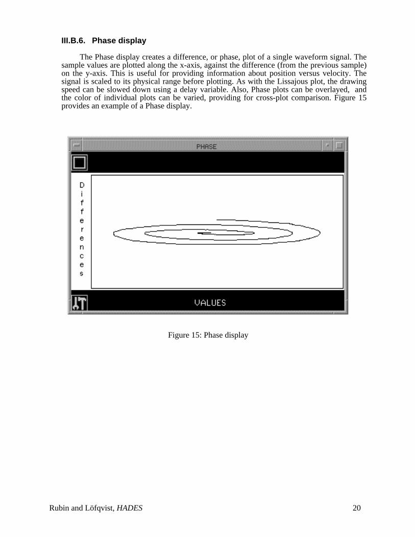
III.B.6. Phase display

The Phase display creates a difference, or phase, plot of a single waveform signal. Thesample values are plotted along the x-axis, against the difference (from the previous sample)on the y-axis. This is useful for providing information about position versus velocity. Thesignal is scaled to its physical range before plotting. As with the Lissajous plot, the drawingspeed can be slowed down using a delay variable. Also, Phase plots can be overlayed, andthe color of individual plots can be varied, providing for cross-plot comparison. Figure 15provides an example of a Phase display.

Figure 15: Phase display


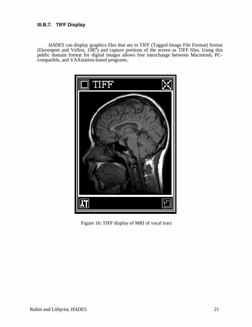
III.B.7. TIFF Display

HADES can display graphics files that are in TIFF (Tagged Image File Format) format(Davenport and Vellon, 1987) and capture portions of the screen as TIFF files. Using thispublic domain format for digital images allows free interchange between Macintosh, PC-compatible, and VAXstation-based programs.

Figure 16: TIFF display of MRI of vocal tract


III.C. Signal measurement

The major use of HADES is the measurement, processing, and analysis of signals.These can be accomplished using the graphical interface, the command line interface, or bycreating custom procedures in the HADES procedural language (SPIEL). This section focuseson signal labelling. Section III.D provides an overview of some of the analysis andprocessing tools. Information about SPIEL including detailed examples can be found inSection IV and Appendix VI.

III.C.1. Labelling signals

Labels represent a way of marking exact locations or a range of values in signals andsampled data files. In this approach a label consists of a name and a set of fields. Each fieldconsists of a field name and an integer, decimal, or string value. Labels may also havecomments. Labels can be represented graphically by a time marker being drawn on thesignal. This marker includes a vertical line that corresponds to the central time value for thelabel and a horizontal bar that specifies the label’s temporal range (see Figure 17).

Labels are stored in ASCII text files and are usually given a name related to thesampled data file or signal they are associated with. For example, if you have a sampled datafile named COW.PCM, then the default label file will be called COW.LAB. However, labelfiles can optionally have any name and can be associated with any signal or file. Each labelmust have a name field that contains the name of the label, and a central time field whosevalue represents its location in the signal. All other fields are optional. Below we havedefined the label fields that are presently supported in HADES.

Field Example Description

CHANNEL CHANNEL=COW Signal that label came from

TIME TIME=1119.4 Center time in msec.

LRANGE LRANGE=300.326 Distance of left edge of selectionfrom center time in msec.

RRANGE RRANGE=235.483 Distance of right edge of selectionfrom center time in msec.

SAMPLE SAMPLE=11195 Sample number of center time

AMPLITUDE AMPLITUDE=75 Value of sample at center time

ATTRIBUTE ATTRIBUTE=0 Controls line drawing type, where: 0 = solid line 1 = dashed line

Labels can either be set from SPIEL, or by working interactively with the data shown ina Display Window. In this latter approach, labels are placed in a number of ways. One way isto choose a location in the signal, using the mouse to move the pointer to the appropriateplace, and then press the right mouse button. This will bring up a dialog box that provides forthe specification of the label name, an alias, times for left and right ranges, and an attributesand comment field. Another method is to choose a location for the cursor, using the mouse,


and pressing the middle button to place the cursor in the signal. Pressing Ctrl-L orchoosing LABEL:SET LABEL from the menu bar will bring up the Label Dialog Box. Anadditional way of marking a label is to use the mouse to select a portion of the signal byclicking and dragging, and then using one of the methods just described to bring up the LabelDialog Box. Labels can also be generated by the Event Marking routines in HADES (seesection III.C.2, below) or can be created using SPIEL procedures. In addition, HADESfunctions are available for retrieving label times and/or name strings. These values can thenbe used in SPIEL procedures to automate processing. Detailed examples of this approach areprovided in section IV.

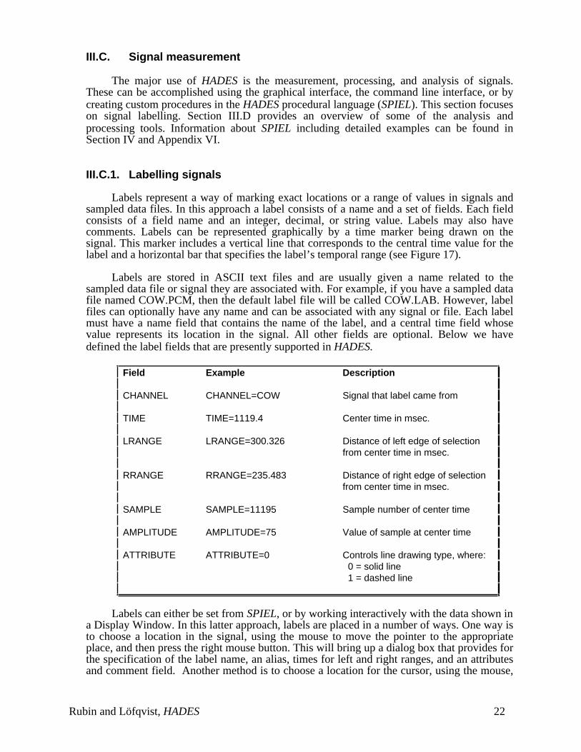
An example of a signal that has been labelled is shown in the figure below. ThisDisplay Window has two panels. The top panel, called OLD, contains the waveform for thesentence “The cow chewed its cud” prior to labelling. The bottom panel, called COW, showsthe results of manually labelling a section of speech. Each word was first selected, a labelwas set near the middle of the selection, and the label was given a name.

Figure 17: Display Window showing a labelled signal

Listing the labels for this signal would show the following information:

LABELS ATTACHED TO SIGNAL COW:

THE: TIME = 313.977 SAMPLE = 3141 LRANGE = 75.082 RRANGE= 75.082 AMP = 101 COW: TIME = 607.478 SAMPLE = 6076 LRANGE = 177.466 RRANGE=150.163 AMP = 75 CHEWED: TIME = 1119.4 SAMPLE = 11195 LRANGE = 300.326 RRANGE=235.483 AMP = 578 ITS: TIME = 1443.61 SAMPLE = 14437 LRANGE = 54.605 RRANGE= 40.954 AMP =-219 CUD: TIME = 1771.24 SAMPLE = 17713 LRANGE = 235.483 RRANGE=228.657 AMP = 82


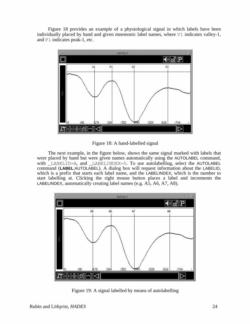
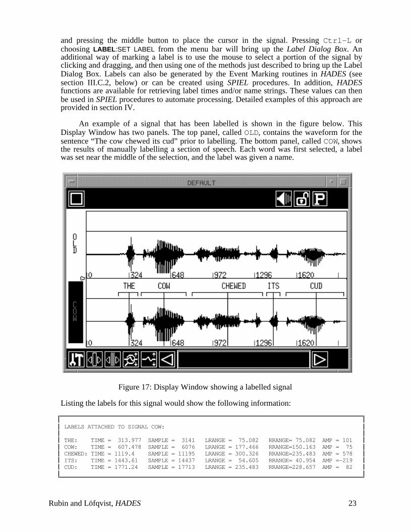
Figure 18 provides an example of a physiological signal in which labels have beenindividually placed by hand and given mnemonic label names, where V1 indicates valley-1,and P1 indicates peak-1, etc.

Figure 18: A hand-labelled signal

The next example, in the figure below, shows the same signal marked with labels thatwere placed by hand but were given names automatically using the AUTOLABEL command,with _LABELID=A, and _LABELINDEX=5. To use autolabelling, select the AUTOLABELcommand (LABEL:AUTOLABEL). A dialog box will request information about the LABELID,which is a prefix that starts each label name, and the LABELINDEX, which is the number tostart labelling at. Clicking the right mouse button places a label and increments theLABELINDEX, automatically creating label names (e.g. A5, A6, A7, A8).

Figure 19: A signal labelled by means of autolabelling


III.C.2. Event marking

Event marking in HADES may be used to label significant events in signals. These eventsinclude:

• peaks

• valleys

• plateaus

• onsets

• offsets

• segments

• zero crossings

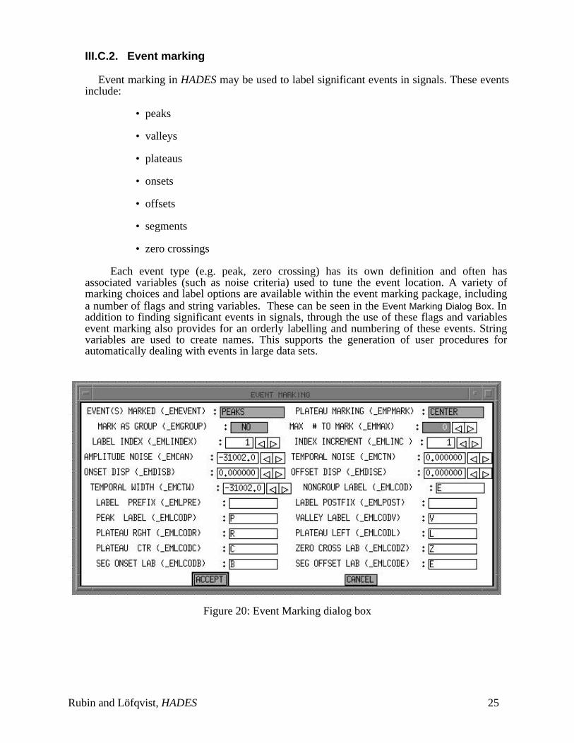
Each event type (e.g. peak, zero crossing) has its own definition and often hasassociated variables (such as noise criteria) used to tune the event location. A variety ofmarking choices and label options are available within the event marking package, includinga number of flags and string variables. These can be seen in the Event Marking Dialog Box. Inaddition to finding significant events in signals, through the use of these flags and variablesevent marking also provides for an orderly labelling and numbering of these events. Stringvariables are used to create names. This supports the generation of user procedures forautomatically dealing with events in large data sets.

Figure 20: Event Marking dialog box


III.D. Signal processing and analysis

III.D.1 Waveform editing and manipulation

HADES can be used, interactively, to graphically edit and manipulate signals. As anexample, this is often done with audio waveforms. The user can CUT, COPY, PASTE,SILENCE, TRIM, portions of the waveform. Effects, such as AMPLIFY, FADEIN, FADEOUT,INVERT, RECTIFY, REVERSE, etc., can be used to provide quick global waveformmanipulations. Audio feedback is available for evaluating the results of these changes. Thisuse of the program is similar to what is now commonly available in desktop soundmanipulation programs, such as the SoundEdit series on the Macintosh and also replaces thefunctionality of the previous waveform manipulation workhorse at Haskins, a programnamed WENDY (Szubowicz, 1982) used heavily during the 1970s and 1980s. Although theuse of HADES in this way seems very similar to the desktop computer programs, they aremany differences. The most important is the accessible and powerful integrated procedurallanguage, SPIEL, which permits custom user-developed procedures that can automaterepetitive signal manipulation in large data sets. SPIEL will be discussed in greater detail insection IV.

III.D.2 Signal processing

A variety of different processing tools are available in HADES. These tools can beaccessed in a variety of ways, including through the menus, the command language, userfunctions, and SPIEL. The signal processing tools include:

• Amplification modifies the energy of the signal or signal portion

• Averaging creates an averaged signal from a set of signals

• DCadd adds a DC constant to all signal values

• Demean the mean of a signal is calculated and then subtracted from all signal values

• Integration calculate the definite integral

• Rectification performs in-place full or half wave rectification

• RMS calculates the RMS (root mean square) energy using the following algorithm: RMS = 20*log10(sqrt(sum1/npts));

where sum1 is the running sum of x*x(where x is an individual data point),and npts is the number of points inthe vector


• Smoothing replaces the signal with a smoothed version using odd-number filters: triangular, rectangular, Hamming, or Hanning

• Filtering creates FIR low-pass and high-pass filters.

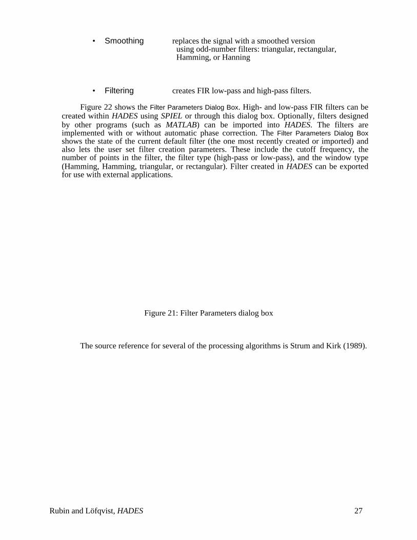
Figure 22 shows the Filter Parameters Dialog Box. High- and low-pass FIR filters can becreated within HADES using SPIEL or through this dialog box. Optionally, filters designedby other programs (such as MATLAB) can be imported into HADES. The filters areimplemented with or without automatic phase correction. The Filter Parameters Dialog Boxshows the state of the current default filter (the one most recently created or imported) andalso lets the user set filter creation parameters. These include the cutoff frequency, thenumber of points in the filter, the filter type (high-pass or low-pass), and the window type(Hamming, Hamming, triangular, or rectangular). Filter created in HADES can be exportedfor use with external applications.

Figure 21: Filter Parameters dialog box

The source reference for several of the processing algorithms is Strum and Kirk (1989).


III.D.3 Spectral analysis

HADES provides for spectral analysis using the Discrete Fourier Transform (DFT) andLinear Predictive Coding (LPC). These techniques are standard approaches for speech andsignal analysis, thus, we will not go into detail about them here. Instead we will focus on howsignal analysis is implemented in HADES and details specific to the HADES environment. Avariety of sources provide additional information on speech analysis. Among others, we referthe reader to Atal, 1985; Fallside, 1985; Fallside & Woods, 1985; Markel & Gray, 1976;O’Shaughnessy, 1988, 1995; Rabiner & Schafer, 1979; and Witten, 1982) .

Within HADES, a number of spectral displays are available, as shown above in sectionIII.B.3, including gray-scale spectrograms, LPC and FBA time-based pseudo-spectrograms,spectral cross-sections, and 3D spectral waterfalls. Additional spectral calculations includethe centroid measure.

Spectral analysis of a signal, based on the Discrete Fourier Transform, can beperformed by HADES, creating a DFT signal which can be displayed or saved. Alternatively,pre-analyzed DFT data can be read in from files saved by HADES. Three global flagvariables are used to control the DFT spectral analysis. The first, _DFTWINT, specifies thetype of window used in the analysis. The size of the analysis window is set by _DFTWINS.The amount (number of points) that the analysis is shifted over for each frame is specified by_DFTSKIP. LPC analysis creates a signal with the same use and privileges as DFT analysis,and also creates an associated FBA signal. The FBA signal was designed by the first authorfor use in a variety of programs at Haskins Laboratories during the 1980s. An FBA file is anASCII file that contains the formant, bandwidth, and amplitude values from an LPC analysisfile created with the ILS program, along with other selected information. The creation of thisfile provided a means for capturing this data and using it without having to remain within theILS framework. DFT, LPC, and FBA signals can be displayed simultaneously in a window,along with a waveform or waveforms. This is useful for direct comparison of the differentanalysis techniques. Figure 21 shows such a window, with a waveform, and DFT, raw LPC(smoothed), and FBA (peak-picked formant center frequencies) displays.

Spectrograms are generated by DFT analysis of the sampled data files using the IEEEpackage of signal processing routines (IEEE, 1979). Our particular implementation is basedon an earlier Haskins program called SPA, written by Richard McGowan and Philip Rubin.As usual, analysis can be procedure-, command-, or menu-driven. When using the menucommand, a dialog box guides the user through the selection of analysis options such assource data file, analysis type, window type and size, starting and ending portions of thewaveform to analyze. Once a spectrogram has been calculated and displayed, the user caninteract with this spectral display. For example, a spectral cross-section can be generatedwhenever there is a mouse click on the spectrogram display. Spectral cross-sections showfrequency-magnitude information for a single frame. A full spectral analysis of a single framecan quickly be obtained by placing a cursor in a waveform and using the SNAPSHOTcommand or menu selection.

An additional spectral measure is the centroid, which is a weighted average ofmagnitudes that is used to define the center of mass over a frequency range. This option maybe selected from the tools menu on the cross-section plot, or used as a typed commandwithout going through the graphical display. If done graphically, the frequency range can beselected with the mouse. The code used to generate the centroid is shown in Appendix V.The inclusion of support for calculating centroids in the HADES program provides a goodexample of how this program has been customized to the particular needs of the Haskinsresearch community. This particular analysis was one that was frequently requested by usersand was of sufficient importance to be included as a HADES primitive. Other less frequently


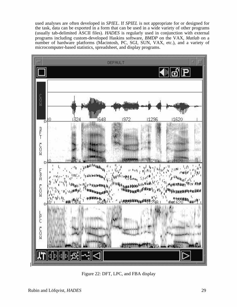
used analyses are often developed in SPIEL. If SPIEL is not appropriate for or designed forthe task, data can be exported in a form that can be used in a wide variety of other programs(usually tab-delimited ASCII files). HADES is regularly used in conjunction with externalprograms including custom-developed Haskins software, BMDP on the VAX, Matlab on anumber of hardware platforms (Macintosh, PC, SGI, SUN, VAX, etc.), and a variety ofmicrocomputer-based statistics, spreadsheet, and display programs.

[

Figure 22: DFT, LPC, and FBA display


III.D.4 Temporal analysis

Several frame-based temporal analyses are available in HADES, including fundamentalfrequency (F0) analysis, energy analysis, and zero-crossing count. Temporal analysis of asignal results in a new signal being generated. This new signal contains a value for eachframe, with a sampling rate adjusted according to the frame size. If temporal analysis isselected via the menu, an additional panel is added to the active display window containing adisplay of the resulting analysis vector. Details about the different analysis types are providedbelow.

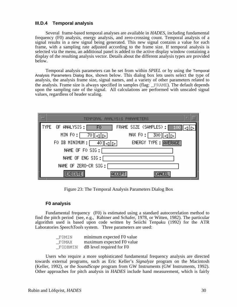
Temporal analysis parameters can be set from within SPIEL or by using the TemporalAnalysis Parameters Dialog Box, shown below. This dialog box lets users select the type ofanalysis, the analysis frame size, signal names, and a variety of other parameters related tothe analysis. Frame size is always specified in samples (flag: _FRAME). The default dependsupon the sampling rate of the signal. All calculations are performed with unscaled signalvalues, regardless of header scaling.

Figure 23: The Temporal Analysis Parameters Dialog Box

F0 analysis

Fundamental frequency (F0) is estimated using a standard autocorrelation method tofind the pitch period (see, e.g., Rabiner and Schafer, 1978, or Witten, 1982). The particularalgorithm used is based upon code written by Seiichi Tenpaku (1992) for the ATRLaboratories SpeechTools system. Three parameters are used:

_F0MIN minimum expected F0 value_F0MAX maximum expected F0 value_F0DBMIN dB level required for F0

Users who require a more sophisticated fundamental frequency analysis are directedtowards external programs, such as Eric Keller’s Signalyze program on the Macintosh(Keller, 1992), or the SoundScope program from GW Instruments (GW Instruments, 1992).Other approaches for pitch analysis in HADES include hand measurement, which is fairly


simple within HADES with a small amount of data, and yields the most accurate results; orautomatic peak picking using the HADES event marking options (see section III.C.2).

Energy analysis

Three types of energy measure are available, selected with the _ENERGY flag:

DB compute 10*log10(average ss )

AVERAGE compute average sum of squares over the frame (default)

PEAK find the peak square over the frame, and normalize to max volts squared, yielding range 0 to 100.

Zero-crossing analysis

A signal vector is created based upon a count of zero-crossings within a pre-definedtemporal window. The zero crossing count can be displayed as a temporal signal. Zero-crossings are a special class of event mentioned about in the Event Marking section (III.C.2).For temporal analysis, the zero-crossing count is defined as:

(# of crossings over midscale within frame)/(sizeof frame)


III.E. Special Features in HADES

III.E.1. Journaling

HADES provides a means for saving the results of certain measurements and includinguser-created comments in an ASCII file. This file is known as the journal file. The processof writing information to this file is called journaling. The user can either open a journal fileof their own choosing or they can use the default file. The default journal file is opened andenabled for writing when a JOURNAL OPEN command is given. Journal files are opened inappend mode, and the program writes the date and time in the journal file upon opening.HADES will automatically write centroid calculations and cross-section cursor values to thejournal file when it is enabled. The SPIEL procedure in section IV.B.4 provides an exampleof how the journal file can be used. In this example, a variety of information is written to thejournal file including tongue receiver positions and displacement, velocity, duration ofmovements, and coding variables for an Analysis of Variance.

III.E.2. Data scaling and calibration

Issues of data scaling and calibration within HADES are of importance in terms of thedisplay, measurement, and comparison of signals. Whether or not signals are scaled isdetermined by the header of the sampled data file (the PCM header). Usually speech isunscaled, and physical data is scaled. Unscaled data always defaults to a range of -2048 to2047. Data in files is stored as short integers in the range 0 to 4095; for scaled data, theheader contains calibration constants which determine the actual range.

Plot scaling options

When data is being plotted, a large number of options are available for controlling howthe actual display looks. This is useful when different signal types are mixed and they need tobe viewed together and compared against each other. The options include the following.

AUTO Scale to the max/min of the panel signal, as specified by its header information.

POOLED Scale to the smallest min/largest max of all the signals in the window, based on their header information.

FIXED Scale to the min/max specified by the window toolbox

UNIQUE Scale to the min/max specified by the panel toolbox

RANGE Scale to a fixed amplitude range (in window toolbox) with a midpoint determined by the min/max of the panel.

The scaling mode for a window is set initially to the default specified in the flag__WINSCALE. This is set to __FIXED at startup, and may be reset by the user: e.g.,__WINSCALE = __AUTO. For a given window, the scaling mode may be changed with thetoolbox.


Signal scaling

Signal values are stored as unsigned integers in the range 0 to 4095. The signals arescaled (or not) according to the values calm and calb in the signal header. Beforeoperations, stored values are converted to floating point:

(stored_value - 2048)*calm + calb

Rescaling after operations

Unscaled signals are never scaled as a result of a HADES operation. By default, scaleddata is automatically rescaled after applying functions, pasting, and math operations, exceptfor the extract function and for pasting into an empty window, in which cases the createdsignal inherits the scaling of its parent. Scaled data is not rescaled after effects.

A user flag has been provided to override the default:

_RESCALE = _NONE (or _OFF) no rescaling: data is clipped. _RESCALE = _ALL (or _ON) always rescale. _RESCALE = _DEFAULT use the default described above.

RESCALING COMMANDS:

RESCALE signal min max flags the header as scaled data,and computes calibration constants(header values cal_m and cal_b) which generate

min and max from stored values 0 and 4095.

UNSCALE signal flags the header as unscaled data, and removesstored scaling parameters from the header.


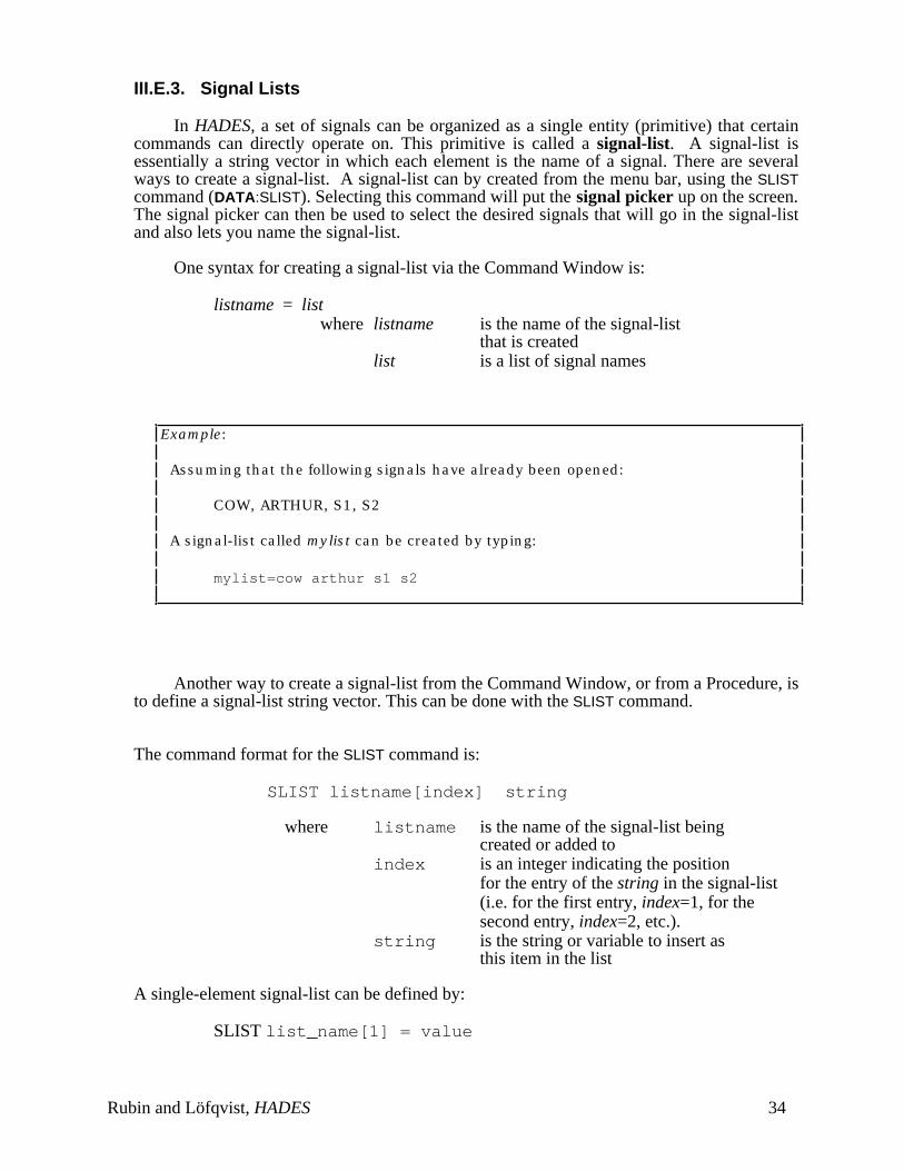
III.E.3. Signal Lists

In HADES, a set of signals can be organized as a single entity (primitive) that certaincommands can directly operate on. This primitive is called a signal-list. A signal-list isessentially a string vector in which each element is the name of a signal. There are severalways to create a signal-list. A signal-list can by created from the menu bar, using the SLISTcommand (DATA:SLIST). Selecting this command will put the signal picker up on the screen.The signal picker can then be used to select the desired signals that will go in the signal-listand also lets you name the signal-list.

One syntax for creating a signal-list via the Command Window is:

listname = list where listname is the name of the signal-list

that is createdlist is a list of signal names

Example:

Assuming that the following signals have already been opened:

COW, ARTHUR, S1, S2

A signal-list called mylist can be created by typing:

mylist=cow arthur s1 s2

Another way to create a signal-list from the Command Window, or from a Procedure, isto define a signal-list string vector. This can be done with the SLIST command.

The command format for the SLIST command is:

SLIST listname[index] string

where listname is the name of the signal-list beingcreated or added to

index is an integer indicating the positionfor the entry of the string in the signal-list(i.e. for the first entry, index=1, for thesecond entry, index=2, etc.).

string is the string or variable to insert asthis item in the list

A single-element signal-list can be defined by:

SLIST list_name[1] = value


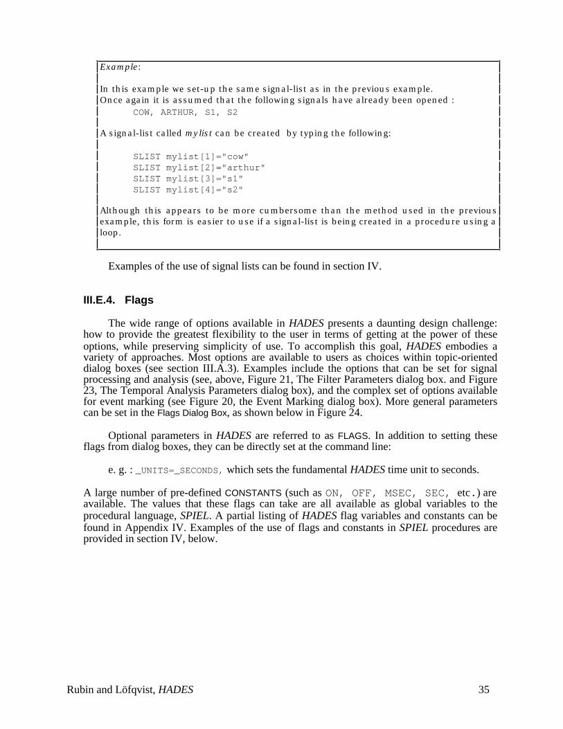
Example:

In this example we set-up the same signal-list as in the previous example.Once again it is assumed that the following signals have already been opened :

COW, ARTHUR, S1, S2

A signal-list called mylist can be created by typing the following:

SLIST mylist[1]="cow"SLIST mylist[2]="arthur"SLIST mylist[3]="s1"SLIST mylist[4]="s2"

Although this appears to be more cumbersome than the method used in the previousexample, this form is easier to use if a signal-list is being created in a procedure using aloop.

Examples of the use of signal lists can be found in section IV.

III.E.4. Flags

The wide range of options available in HADES presents a daunting design challenge:how to provide the greatest flexibility to the user in terms of getting at the power of theseoptions, while preserving simplicity of use. To accomplish this goal, HADES embodies avariety of approaches. Most options are available to users as choices within topic-orienteddialog boxes (see section III.A.3). Examples include the options that can be set for signalprocessing and analysis (see, above, Figure 21, The Filter Parameters dialog box. and Figure23, The Temporal Analysis Parameters dialog box), and the complex set of options availablefor event marking (see Figure 20, the Event Marking dialog box). More general parameterscan be set in the Flags Dialog Box, as shown below in Figure 24.

Optional parameters in HADES are referred to as FLAGS. In addition to setting theseflags from dialog boxes, they can be directly set at the command line:

e. g. : _UNITS=_SECONDS, which sets the fundamental HADES time unit to seconds.

A large number of pre-defined CONSTANTS (such as ON, OFF, MSEC, SEC, etc.) areavailable. The values that these flags can take are all available as global variables to theprocedural language, SPIEL. A partial listing of HADES flag variables and constants can befound in Appendix IV. Examples of the use of flags and constants in SPIEL procedures areprovided in section IV, below.


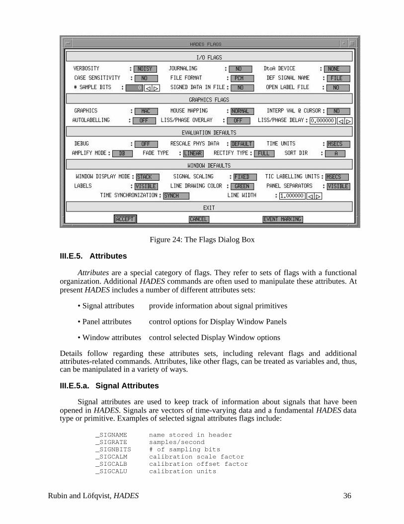
Figure 24: The Flags Dialog Box

III.E.5. Attributes

Attributes are a special category of flags. They refer to sets of flags with a functionalorganization. Additional HADES commands are often used to manipulate these attributes. Atpresent HADES includes a number of different attributes sets:

• Signal attributes provide information about signal primitives

• Panel attributes control options for Display Window Panels

• Window attributes control selected Display Window options

Details follow regarding these attributes sets, including relevant flags and additionalattributes-related commands. Attributes, like other flags, can be treated as variables and, thus,can be manipulated in a variety of ways.

III.E.5.a. Signal Attributes

Signal attributes are used to keep track of information about signals that have beenopened in HADES. Signals are vectors of time-varying data and a fundamental HADES datatype or primitive. Examples of selected signal attributes flags include:

_SIGNAME name stored in header _SIGRATE samples/second

_SIGNBITS # of sampling bits _SIGCALM calibration scale factor _SIGCALB calibration offset factor _SIGCALU calibration units


_SIGDFTHEAD DFT head in msec _SIGDFTTAIL DFT tail in msec _SIGDFTWS size of the DFT window _SIGDFTWT type of analysis window _SIGDFTWSK skip size (time resolution) _SIGDFTLPC name of the associated LPC or DFT signal _SIGDFTFBA name of the associated FBA signal

These values always refer to the current active signal, and are reloaded every time a newactive signal is selected. A dialog box, under the DATA menu, displays the current values,allowing resetting of the relevant attributes. The dialog box also permits the selection of othersignals for attribute display, with an option for resetting the active signal.

HADES includes several special purpose commands related to signal attributes.These commands are:

LIST SIGATT signalname lists the attributes of the named signal

JOURNAL SIGATT signalname journals the attributes of the named signal

CSIGATT sig1 sig2 copies the attributes from sig1 to sig2

SIGATT sig attribute value sets the attribute value for named signal

III.E.5.b. Window Attributes

Window attributes are used to control selected Display Window options. The basicwindow attributes command is:

WINDOW attribute [=] value

which will change window attributes after the window has been drawn.

Window attributes include:

SYNCH sets time synchronization of the windowMAX sets the upper limit for fixed data scalingMIN set lower limit for fixed scalingRANGE sets the range for fixed-range scalingMODE sets _OVERLAY or _STACK modeSCALE sets the data scaling options

III.E.5.c. Panel Attributes

Temporal displays can have more than one signal displayed in a window. In general,each signal is displayed in a separate panel, unless the overlay option has been selected. Awide variety of options is available for controlling the appearance of panels and the datawithin panels. The basic panel attribute command is:

PANEL # attribute [=] value

This command operates on a default panel list (plist), which is a HADES data structure thatspecifies a list of panel names. The panel list is basically a vector of strings. If no panel lists


have been specifically created (see PLIST and CREATE commands, described below), thedefault panel list will be the panel list in the active window. Otherwise, the default panel listwill be the one named in the global variable _PLIST .

A panel number (#) identifies which panel in the list is affected by the command.Panels are counted from 1, starting at the top of the display.

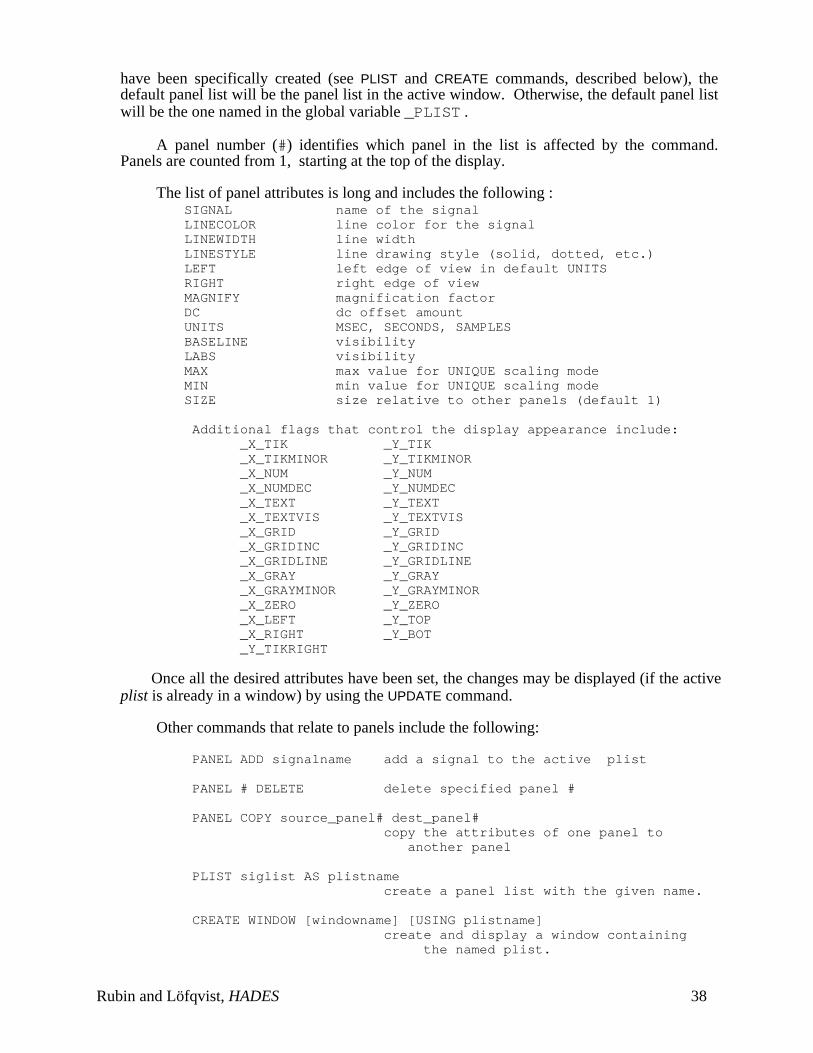
The list of panel attributes is long and includes the following : SIGNAL name of the signal LINECOLOR line color for the signal LINEWIDTH line width LINESTYLE line drawing style (solid, dotted, etc.) LEFT left edge of view in default UNITS RIGHT right edge of view MAGNIFY magnification factor DC dc offset amount UNITS MSEC, SECONDS, SAMPLES BASELINE visibility LABS visibility MAX max value for UNIQUE scaling mode MIN min value for UNIQUE scaling mode SIZE size relative to other panels (default 1)

Additional flags that control the display appearance include: _X_TIK _Y_TIK _X_TIKMINOR _Y_TIKMINOR _X_NUM _Y_NUM _X_NUMDEC _Y_NUMDEC _X_TEXT _Y_TEXT _X_TEXTVIS _Y_TEXTVIS _X_GRID _Y_GRID _X_GRIDINC _Y_GRIDINC _X_GRIDLINE _Y_GRIDLINE _X_GRAY _Y_GRAY _X_GRAYMINOR _Y_GRAYMINOR _X_ZERO _Y_ZERO _X_LEFT _Y_TOP _X_RIGHT _Y_BOT _Y_TIKRIGHT

Once all the desired attributes have been set, the changes may be displayed (if the activeplist is already in a window) by using the UPDATE command.

Other commands that relate to panels include the following:

PANEL ADD signalname add a signal to the active plist

PANEL # DELETE delete specified panel #

PANEL COPY source_panel# dest_panel# copy the attributes of one panel to

another panel

PLIST siglist AS plistname create a panel list with the given name.

CREATE WINDOW [windowname] [USING plistname] create and display a window containing

the named plist.


CREATE PLIST [plistname] [FROM windowname] create a plist from a window

UPDATE redraw all windows containing active plist

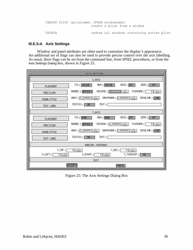
III.E.5.d. Axis Settings

Window and panel attributes are often used to customize the display’s appearance.An additional set of flags can also be used to provide precise control over the axis labelling.As usual, these flags can be set from the command line, from SPIEL procedures, or from theAxis Settings Dialog Box, shown in Figure 25.

Figure 25: The Axis Settings Dialog Box


III.E.6. Importing and Exporting Data

HADES supports a variety of alternate file formats for inputting and outputting data.The native file format for sampled data (or other time-varying) signals at HaskinsLaboratories has been in use for over twenty years and is called the PCM format (Whalen etal, 1990). HADES also supports several additional sampled data formats, including ILS,STM, and ASCII. The default file format may be set from the Flags Dialog Box.

ILS format refers to sampled data created by standard ILS, a commercial signalprocessing system developed by STI. (Haskins implementation of the ILS systems hasmodified it to deal with PCM format). ILS analysis files are not supported. The STM formatwas developed at the Indiana University Psychology Department Speech Lab. Non-integralsampling rates are supported only by PCM format. STM format supports only 10,000 Hz and20,000 Hz sampling rates.

HADES handles data with amplitude resolutions other than 12 sample bits in the analogto digital conversion. Values from 1 to 16 are allowed. A global variable, _NBITS,determines this resolution. Bit resolution is stored as part of the signal header, therebysupporting different resolutions for different signals. The default, _NBITS =0, checks the fileheader for bit information, setting the number of bits for the signal (the signal nbits) to 12 ifnone is found. If _NBITS is set to a nonzero value, the signal nbits will be set to _NBITSregardless of header specification. Sample values are assumed to be stored in the range 0 to2**(_NBITS)-1. Amplitudes are calculated with an offset of 2**(_NBITS-1), after whichphysical scaling, if any, is applied.

The main interchange format in HADES is in the form of ASCII files. In addition tosampled data, data can be exported from HADES as a journal file, which records selectedmeasurements and saves them in an ASCII file (see section III.E.1). Label files (see sectionIII.C.1) are also saved in ASCII format. However, the most powerful use of ASCII exportinvolves creating SPIEL procedures to format and save the results of HADES analyses andmeasurements. Detailed examples of such procedures are provided in section IV, below. Thistechnique makes HADES compatible with a wide variety of workstation and desktopcomputer programs for statistics, data manipulation, and data plotting.


IV. SPIEL

While most of the commands and functions in HADES can be executed from the menusor the keyboard, significant amounts of time and effort can be saved by creating procedures thatare used to help automate the repetitive processing of signals. To accomplish this, HADESincorporates a procedural language called SPIEL (Signal Processing Interactive EditingLanguage) that allows the user to create customized routines used for the processing of the datafrom experiments.

IV.A. The SPIEL language

SPIEL is the procedurally-oriented programming language that is an intrinsic part ofHADES. Procedures can be created that take advantage of most of the structures of HADES,including commands, command-line entry of values, variables, and data structures. In addition,there are facilities of HADES that are specific to SPIEL, such as conditionals and loopingstructures. A listing of HADES commands can be found in Appendix II and functions inAppendix III.

IV.A.1 Mathematical, logical, and comparison primitives

MATHEMATICAL OPERATORS

+ addition- subtraction* multiplication/ division^ exponentiation

MATHEMATICAL FUNCTIONS

ABS absolute valueCOS cosineMAX maximum of a scalarMIN minimum of a scalarSIN sineSQR squareSQRT square rootTAN tangent

LOGICAL OPERATORS

NOT NOTOR ORAND AND


COMPARISON OPERATORS

== equal to< less than<= less than or equal to> greater than>= greater than or equal to<> not equal to

RESERVED CHARACTERS

( ) demarcation of PROCEDURE arguments;mathematical grouping

[ ] indexing of signal and vector elements

IV.A.2. Control structures

SPIEL provides control structures for conditional branching and conditional looping. Thefirst, the IF — END IF structure, executes a statement or set of statements if a particular conditionis met. Conditions may be built using comparative operators. The general form of the IF structureis:

IF (condition)statement..

END IF

The second control structure, the WHILE — END WHILE, executes a statement or set ofstatements while a particular condition is true. Conditions may be built using comparativeoperators. WHILE structures are useful for creating loops. The general form of the WHILEstructure is:

WHILE (condition)statement..

END WHILE

The FOR — END FOR loops through a series of statements, incrementing an index, andchecking to see if this index is within the range specified by the user. The general form of theFOR structure is:

FOR index = val1 TO val2 { STEP val3 }statement..

END FOR


IV.A.3. Miscellaneous

Keyboard input in procedures is provided by the GET command. Its format is:

GET “prompt” varlist

The text of the prompt is printed and the user enters the variables of the varlist.

The FSLIST command creates a signal list by reading an ASCII file containing the namesof signals. It has the form:

FSLIST filename listname

The filename is the name of the ASCII file containing the list of signal names and the listname isthe name that will be given to the signal list.

IV.B. SPIEL examples

The following sections provide examples of procedures written in SPIEL. These arebased on a set of routines that has been developed to process two-dimensional movement signalsrecorded using an electromagnetic transduction technique. As a background to the presentationof the SPIEL routines, a brief description of the characteristics of the movement signals will beprovided first.

IV.B.1. Signals and signal naming conventions

Movement signals were recorded using a three-coil transmitter system described byPerkell, et al., (1992). Further details about the experimental procedures can be found in Löfqvistand Gracco (1994), and Löfqvist, Gracco, and Nye (1993). Receivers were placed on the upperand lower lips, the lower incisors, and at four positions on the tongue. For the sake ofconvenience, the tongue receivers will be referred to by their locations as tongue tip (tt), tongueblade (tbl), tongue body (tb), and tongue root (tr), although we acknowledge that the boundariesbetween these parts of the tongue are imprecise, and the receiver referred to as “tongue root”actually has a higher and more forward position than is customary for that location. In addition,receivers placed on the bridge of the nose and on the upper incisors were used for correction ofhead movements. All data were subsequently corrected for head movements, and then rotatedand translated to bring the occlusal plane into coincidence with the x axis. The linguistic materialconsisted of VCV sequences with all possible combinations of the vowels /i, a, u/ and the stopconsonants /p, t, k, b, d, g/. The sequences were placed in the carrier phrase “Say ... again” withsentence stress occurring on the second vowel of the VCV sequence. Ten tokens of eachsequence were recorded at self-selected speaking rates and intensity levels. The articulatorymovement signals (induced voltages from the receiver coils) were sampled at 625 Hz after low-pass filtering at 200 Hz. The speech signal was pre-emphasized, low-pass filtered at 9.5 kHz andsampled at 20 kHz. The resolution for all signals was 12 bits. After voltage-to-distanceconversion, the movement signals were low-pass filtered using a 25-point triangular windowwith a 3 dB cutoff at 18 Hz. To obtain instantaneous velocity, the first derivative of the positionsignals was calculated using a 3-point central difference algorithm. The velocity signals weresmoothed using the same triangular window.


The files containing the individual signals are identified by utterance number, tokennumber and signal name; the file extension is .PCM. Thus, the file U3T5TBY.PCM contains thevertical tongue body receiver signal for token 5 of utterance 1, while U45T8TTVX.PCMcontains the horizontal velocity of the tongue tip receiver for token 8 of utterance 45. Figure 14shows a plot of receiver trajectories for the sequence /aka/. The subject is facing to the left. Atracing of the hard palate is also shown.

IV.B.2. Creating tangential velocity signals

One particular problem in analyzing two-dimensional movements is locating the properpoints in time for making measurements. In the analysis of one-dimensional movements, thesepoints are usually identified by zero crossings in the first derivative of the position signal, i.e.,velocity. For two-dimensional movements, marking zero crossings separately in the horizontaland vertical velocity signals usually results in those points occurring at different times. The

preferable solution is to use tangential velocity, defined as = ( ˙ x 2 + ˙ y 2) , where ˙ x ishorizontal velocity and ˙ y is vertical velocity, for locating measurement points, since it is basedon both the horizontal and vertical components of the movement (cf. Löfqvist, Gracco & Nye,1993). The following procedure reads in velocity signal files for all tongue receivers of thespecified tokens for a specified utterance and creates the corresponding tangential velocitysignals. These signals are then saved into files with the proper file names.

Before this procedure is executed, three steps have been taken.The two signal lists mylist and tonguetanlist have been created from two ASCII files asfollows:

fslist siglist.txt mylistfslist tanvel.txt tonguetanlist

The list mylist contains names of signals and is reprinted here, since it will be used in allthe following procedures.

SIGLIST.TXT

1 audio audio signal2 ulx upper lip horizontal position3 ulvx upper lip horizontal velocity4 uly upper lip vertical position5 ulvy upper lip vertical velocity6 llx lower lip horizontal position7 llvx lower lip horizontal velocity8 lly lower lip vertical position9 llvy lower lip vertical velocity10 jawx jaw horizontal position11 jawvx jaw horizontal velocity12 jawy jaw vertical position13 jawvy jaw vertical velocity14 ttx tongue tip horizontal position15 ttvx tongue tip horizontal velocity16 tty tongue tip vertical position17 ttvy tongue tip vertical velocity18 tblx tongue blade horizontal position19 tblvx tongue blade horizontal velocity20 tbly tongue blade vertical position21 tblvy tongue blade vertical velocity


22 tbx tongue body horizontal position23 tbvx tongue body horizontal velocity24 tby tongue body vertical position25 tbvy tongue body vertical velocity26 trx tongue root horizontal position27 trvx tongue root horizontal velocity28 try tongue root vertical position29 trvy tongue root vertical velocity30 ttvtan tongue tip tangential velocity31 ttcurv tongue tip curvature32 tblvtan tongue blade tangential velocity33 tblcurv tongue blade curvature34 tbvtan tongue body tangential velocity35 tbcurv tongue body curvature36 trvtan tongue root tangential velocity37 trcurv tongue root curvature38 ulvtan upper lip tangential velocity39 llvtan lower lip tangential velocity40 jawvtan jaw tangential velocity

In order the create a pathname to locate files, the first part of a VAX VMS disk directoryname has been created:

dirprefix=TU$1:[LOFQUIST.MAGAL.U

Once the procedure has been created, its name will be placed in the HADES Piconwindow which can be configured to contain a clickable list of procedure names. Prior to runningthe procedure described below, the Picon has to be cleared and set to the tear-off mode, so that itwill appear as a tear-off menu:

picon clear_piconwin=_tearoff

In the procedure listed below, everything on a line after the character “!” is ignored. Thecomments on the right of each line have been added here to help in interpreting the statements.

Note that in the following procedures, which will be explained in some detail, largeportions of the code are dedicated to the manipulation of strings to create directory and filenames.


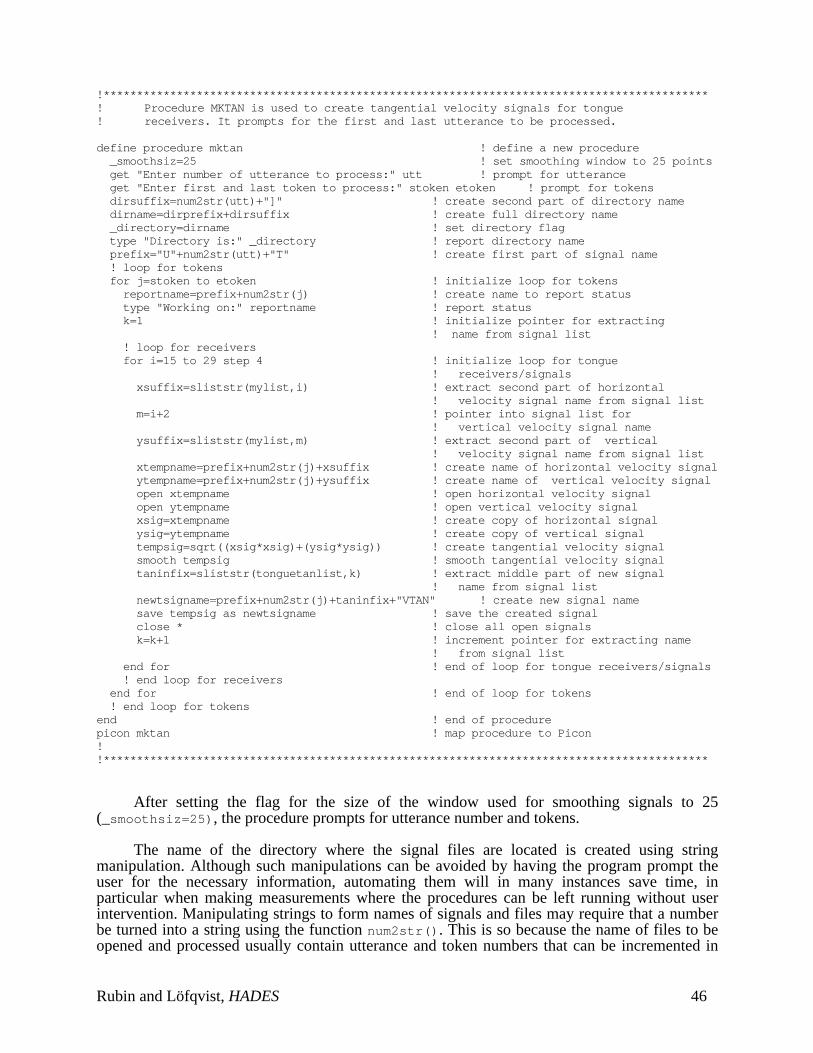
!*******************************************************************************************! Procedure MKTAN is used to create tangential velocity signals for tongue ! receivers. It prompts for the first and last utterance to be processed.

define procedure mktan ! define a new procedure _smoothsiz=25 ! set smoothing window to 25 points get "Enter number of utterance to process:" utt ! prompt for utterance get "Enter first and last token to process:" stoken etoken ! prompt for tokens dirsuffix=num2str(utt)+"]" ! create second part of directory name dirname=dirprefix+dirsuffix ! create full directory name _directory=dirname ! set directory flag type "Directory is:" _directory ! report directory name prefix="U"+num2str(utt)+"T" ! create first part of signal name ! loop for tokens for j=stoken to etoken ! initialize loop for tokens reportname=prefix+num2str(j) ! create name to report status type "Working on:" reportname ! report status k=1 ! initialize pointer for extracting

! name from signal list ! loop for receivers for i=15 to 29 step 4 ! initialize loop for tongue

! receivers/signals xsuffix=sliststr(mylist,i) ! extract second part of horizontal

! velocity signal name from signal list m=i+2 ! pointer into signal list for

! vertical velocity signal name ysuffix=sliststr(mylist,m) ! extract second part of vertical

! velocity signal name from signal list xtempname=prefix+num2str(j)+xsuffix ! create name of horizontal velocity signal ytempname=prefix+num2str(j)+ysuffix ! create name of vertical velocity signal open xtempname ! open horizontal velocity signal open ytempname ! open vertical velocity signal xsig=xtempname ! create copy of horizontal signal ysig=ytempname ! create copy of vertical signal tempsig=sqrt((xsig*xsig)+(ysig*ysig)) ! create tangential velocity signal smooth tempsig ! smooth tangential velocity signal taninfix=sliststr(tonguetanlist,k) ! extract middle part of new signal

! name from signal list newtsigname=prefix+num2str(j)+taninfix+"VTAN" ! create new signal name save tempsig as newtsigname ! save the created signal close * ! close all open signals k=k+1 ! increment pointer for extracting name

! from signal list end for ! end of loop for tongue receivers/signals ! end loop for receivers end for ! end of loop for tokens ! end loop for tokensend ! end of procedurepicon mktan ! map procedure to Picon!!*******************************************************************************************

After setting the flag for the size of the window used for smoothing signals to 25(_smoothsiz=25), the procedure prompts for utterance number and tokens.

The name of the directory where the signal files are located is created using stringmanipulation. Although such manipulations can be avoided by having the program prompt theuser for the necessary information, automating them will in many instances save time, inparticular when making measurements where the procedures can be left running without userintervention. Manipulating strings to form names of signals and files may require that a numberbe turned into a string using the function num2str(). This is so because the name of files to beopened and processed usually contain utterance and token numbers that can be incremented in


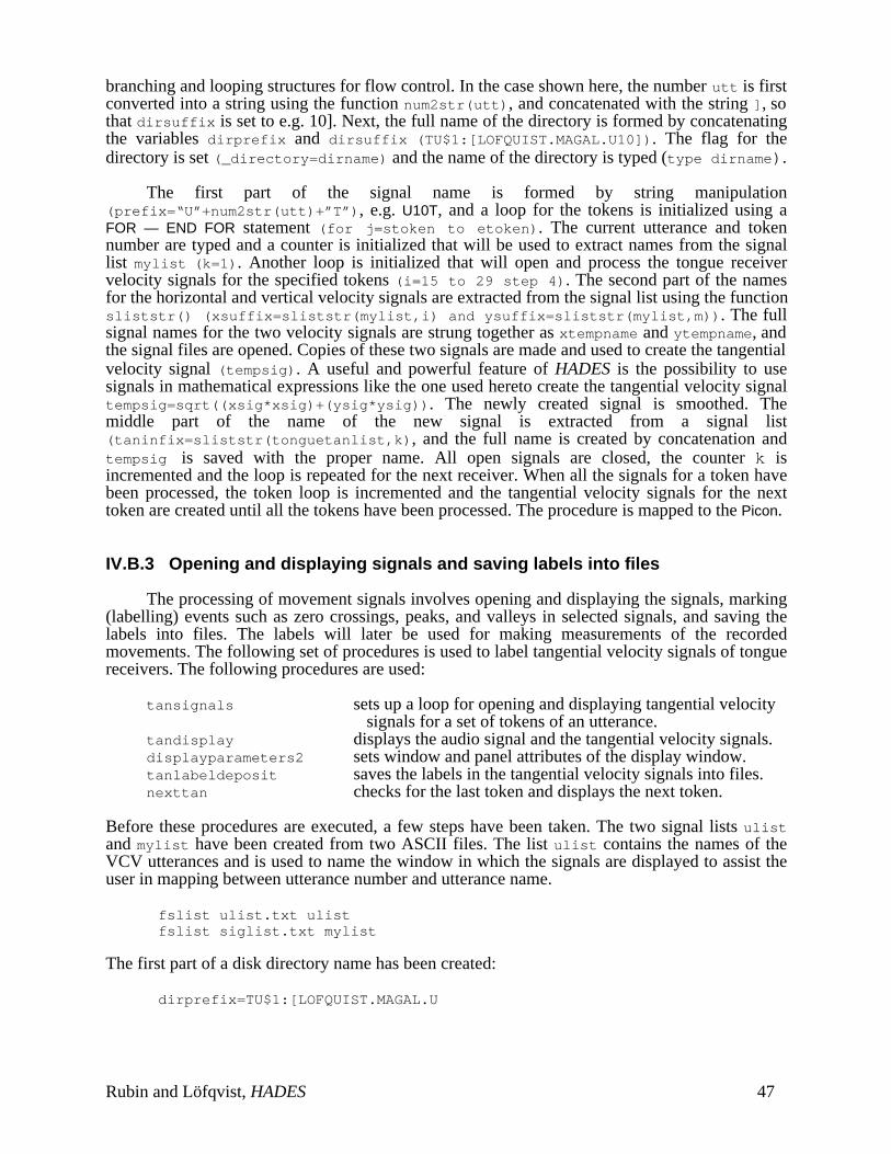
branching and looping structures for flow control. In the case shown here, the number utt is firstconverted into a string using the function num2str(utt), and concatenated with the string ], sothat dirsuffix is set to e.g. 10]. Next, the full name of the directory is formed by concatenatingthe variables dirprefix and dirsuffix (TU$1:[LOFQUIST.MAGAL.U10]). The flag for thedirectory is set (_directory=dirname) and the name of the directory is typed (type dirname).

The first part of the signal name is formed by string manipulation(prefix=“U”+num2str(utt)+”T”), e.g. U10T, and a loop for the tokens is initialized using aFOR — END FOR statement (for j=stoken to etoken). The current utterance and tokennumber are typed and a counter is initialized that will be used to extract names from the signallist mylist (k=1). Another loop is initialized that will open and process the tongue receivervelocity signals for the specified tokens (i=15 to 29 step 4). The second part of the namesfor the horizontal and vertical velocity signals are extracted from the signal list using the functionsliststr() (xsuffix=sliststr(mylist,i) and ysuffix=sliststr(mylist,m)). The fullsignal names for the two velocity signals are strung together as xtempname and ytempname, andthe signal files are opened. Copies of these two signals are made and used to create the tangentialvelocity signal (tempsig). A useful and powerful feature of HADES is the possibility to usesignals in mathematical expressions like the one used hereto create the tangential velocity signaltempsig=sqrt((xsig*xsig)+(ysig*ysig)). The newly created signal is smoothed. Themiddle part of the name of the new signal is extracted from a signal list(taninfix=sliststr(tonguetanlist,k), and the full name is created by concatenation andtempsig is saved with the proper name. All open signals are closed, the counter k isincremented and the loop is repeated for the next receiver. When all the signals for a token havebeen processed, the token loop is incremented and the tangential velocity signals for the nexttoken are created until all the tokens have been processed. The procedure is mapped to the Picon.

IV.B.3 Opening and displaying signals and saving labels into files

The processing of movement signals involves opening and displaying the signals, marking(labelling) events such as zero crossings, peaks, and valleys in selected signals, and saving thelabels into files. The labels will later be used for making measurements of the recordedmovements. The following set of procedures is used to label tangential velocity signals of tonguereceivers. The following procedures are used:

tansignals sets up a loop for opening and displaying tangential velocity signals for a set of tokens of an utterance.

tandisplay displays the audio signal and the tangential velocity signals.displayparameters2 sets window and panel attributes of the display window.tanlabeldeposit saves the labels in the tangential velocity signals into files.nexttan checks for the last token and displays the next token.

Before these procedures are executed, a few steps have been taken. The two signal lists ulistand mylist have been created from two ASCII files. The list ulist contains the names of theVCV utterances and is used to name the window in which the signals are displayed to assist theuser in mapping between utterance number and utterance name.

fslist ulist.txt ulistfslist siglist.txt mylist

The first part of a disk directory name has been created:

dirprefix=TU$1:[LOFQUIST.MAGAL.U


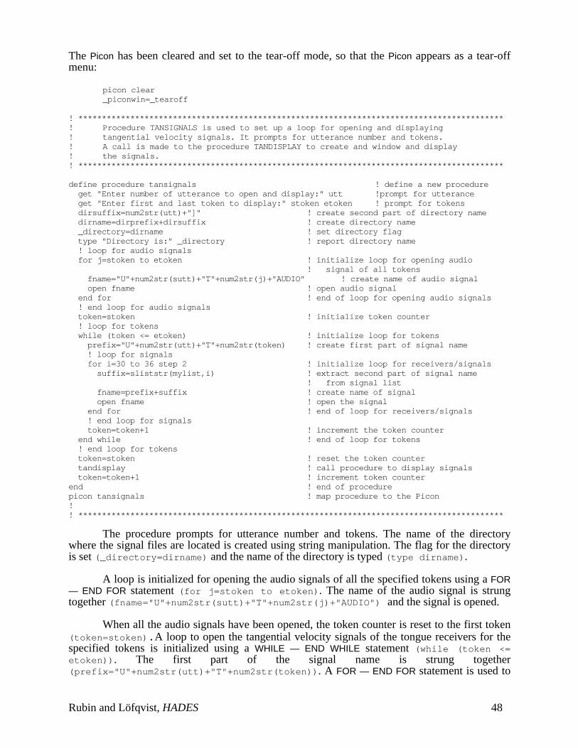
The Picon has been cleared and set to the tear-off mode, so that the Picon appears as a tear-offmenu:

picon clear_piconwin=_tearoff

! ******************************************************************************************! Procedure TANSIGNALS is used to set up a loop for opening and displaying! tangential velocity signals. It prompts for utterance number and tokens.! A call is made to the procedure TANDISPLAY to create and window and display! the signals.! ******************************************************************************************

define procedure tansignals ! define a new procedure get "Enter number of utterance to open and display:" utt !prompt for utterance get "Enter first and last token to display:" stoken etoken ! prompt for tokens dirsuffix=num2str(utt)+"]" ! create second part of directory name dirname=dirprefix+dirsuffix ! create directory name _directory=dirname ! set directory flag type "Directory is:" _directory ! report directory name ! loop for audio signals for j=stoken to etoken ! initialize loop for opening audio

! signal of all tokens fname="U"+num2str(sutt)+"T"+num2str(j)+"AUDIO" ! create name of audio signal open fname ! open audio signal end for ! end of loop for opening audio signals ! end loop for audio signals token=stoken ! initialize token counter ! loop for tokens while (token <= etoken) ! initialize loop for tokens prefix="U"+num2str(utt)+"T"+num2str(token) ! create first part of signal name ! loop for signals for i=30 to 36 step 2 ! initialize loop for receivers/signals suffix=sliststr(mylist,i) ! extract second part of signal name

! from signal list fname=prefix+suffix ! create name of signal open fname ! open the signal end for ! end of loop for receivers/signals ! end loop for signals token=token+1 ! increment the token counter end while ! end of loop for tokens ! end loop for tokens token=stoken ! reset the token counter tandisplay ! call procedure to display signals token=token+1 ! increment token counterend ! end of procedurepicon tansignals ! map procedure to the Picon!! ******************************************************************************************

The procedure prompts for utterance number and tokens. The name of the directorywhere the signal files are located is created using string manipulation. The flag for the directoryis set (_directory=dirname) and the name of the directory is typed (type dirname).

A loop is initialized for opening the audio signals of all the specified tokens using a FOR— END FOR statement (for j=stoken to etoken). The name of the audio signal is strungtogether (fname="U"+num2str(sutt)+"T"+num2str(j)+"AUDIO") and the signal is opened.

When all the audio signals have been opened, the token counter is reset to the first token(token=stoken).A loop to open the tangential velocity signals of the tongue receivers for thespecified tokens is initialized using a WHILE — END WHILE statement (while (token <=etoken)). The first part of the signal name is strung together(prefix="U"+num2str(utt)+"T"+num2str(token)). A FOR — END FOR statement is used to


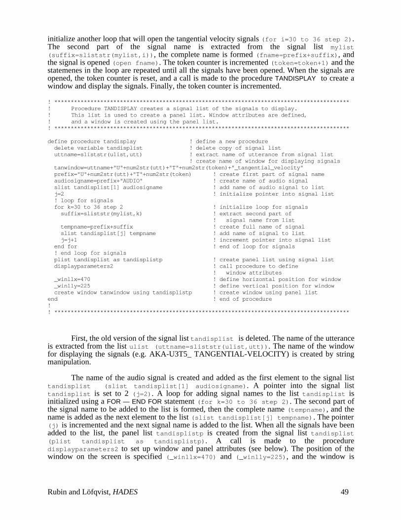
initialize another loop that will open the tangential velocity signals (for i=30 to 36 step 2).The second part of the signal name is extracted from the signal list mylist(suffix=sliststr(mylist,i)), the complete name is formed (fname=prefix+suffix), andthe signal is opened (open fname). The token counter is incremented (token=token+1) and thestatemenes in the loop are repeated until all the signals have been opened. When the signals areopened, the token counter is reset, and a call is made to the procedure TANDISPLAY to create awindow and display the signals. Finally, the token counter is incremented.

! ******************************************************************************************! Procedure TANDISPLAY creates a signal list of the signals to display.! This list is used to create a panel list. Window attributes are defined,! and a window is created using the panel list.! ******************************************************************************************

define procedure tandisplay ! define a new procedure delete variable tandisplist ! delete copy of signal list uttname=sliststr(ulist,utt) ! extract name of utterance from signal list

! create name of window for displaying signals tanwindow=uttname+"U"+num2str(utt)+"T"+num2str(token)+"_tangential_velocity" prefix="U"+num2str(utt)+"T"+num2str(token) ! create first part of signal name audiosigname=prefix+"AUDIO" ! create name of audio signal slist tandisplist[1] audiosigname ! add name of audio signal to list j=2 ! initialize pointer into signal list ! loop for signals for k=30 to 36 step 2 ! initialize loop for signals suffix=sliststr(mylist,k) ! extract second part of

! signal name from list tempname=prefix+suffix ! create full name of signal slist tandisplist[j] tempname ! add name of signal to list j=j+1 ! increment pointer into signal list end for ! end of loop for signals ! end loop for signals plist tandisplist as tandisplistp ! create panel list using signal list displayparameters2 ! call procedure to define

! window attributes _winllx=470 ! define horizontal position for window _winlly=225 ! define vertical position for window create window tanwindow using tandisplistp ! create window using panel listend ! end of procedure!! ******************************************************************************************

First, the old version of the signal list tandisplist is deleted. The name of the utteranceis extracted from the list ulist (uttname=sliststr(ulist,utt)). The name of the windowfor displaying the signals (e.g. AKA-U3T5_ TANGENTIAL-VELOCITY) is created by stringmanipulation.

The name of the audio signal is created and added as the first element to the signal listtandisplist (slist tandisplist[1] audiosigname). A pointer into the signal listtandisplist is set to 2 (j=2). A loop for adding signal names to the list tandisplist isinitialized using a FOR — END FOR statement (for k=30 to 36 step 2). The second part ofthe signal name to be added to the list is formed, then the complete name (tempname), and thename is added as the next element to the list (slist tandisplist[j] tempname). The pointer(j) is incremented and the next signal name is added to the list. When all the signals have beenadded to the list, the panel list tandisplistp is created from the signal list tandisplist(plist tandisplist as tandisplistp). A call is made to the proceduredisplayparameters2 to set up window and panel attributes (see below). The position of thewindow on the screen is specified (_winllx=470) and (_winlly=225), and the window is


created with the proper name using the panel list tandisplistp (create window tanwindowusing tandisplistp).

! ******************************************************************************************! Procedure DISPLAYPARAMETERS2 sets up display parameters for time plots.! ******************************************************************************************

define procedure displayparameters2 ! define a new procedure _x_grid=_off ! turn off horizontal grid in all panels _x_gridinc=100 ! set horizontal tick spacing to 100 ms _x_tik=_inside ! place horizontal tick marks inside panel _x_num=_outside ! place horizontal tick labels outside panel _x_numdec=0 ! set number of decimals in horizontal tick

! labels to 0 _y_grid=_off ! turn off vertical grid in all panels _y_tik=_outside ! place vertical tick marks outside panel _y_num=_outside ! place vertical tick marks outside panel _y_numdec=1 ! set number of decimals in horizontal tick

! labels to 1 _linecolor=_black ! set line color for signals to black _winhigh=800 ! define height of display window on screen _winwide=600 ! define height of display window on screenend ! end of procedure!! ******************************************************************************************

Figure 26 shows a window that has been created using the procedure TANDISPLAY. Theutterance is “Say aka again”. The signal at the top is the audio signal. The tangential velocitysignals are from receivers placed on the tongue tip, the tongue blade, the tongue body, and thetongue root.


Figure 26: Example of a window created using the procedure TANDISPLAY.The signals are from top to bottom, audio, tangential velocity of

tongue tip, tongue blade, tongue body, and tongue root.

Peaks and valleys in the tangential velocity signals are labeled using the event markingroutines of HADES. An example of signals with such labels is shown in Figure 27, below. Thelabels have been placed at three minima of tangential velocity, V1, V2, V3, and at two peaks oftangential velocity, P1, P2. The three labels at the valleys occur during the diphthong in “say”(V1), the first vowel in “aka” (V2), and during the stop closure for the velar stop consonant /k/ in“aka” (V3). The two labels at the peaks occur during the movement from the diphthong in “say”to the first vowel in “aka” (P1), and from the first vowel in “aka” to the velar stop consonant /k/in “aka” (P2). The placement of these labels has been made to examine movement characteristicsin VCV sequences as a function of the identity of the first and second vowels and the middleconsonant (see Löfqvist and Gracco (1994) for further details).


Figure 27: The same display as in Figure 26 with labels in the tangential velocity signals.

The labels are saved into files using the procedure TANLABELDEPOSIT.

! ******************************************************************************************! Procedure TANLABELDEPOSIT saves labels in tangential velocity tongue! receiver signals into files with name of the signal and the extension .LAB.! ******************************************************************************************

define procedure tanlabeldeposit ! define a new procedure ! loop for signals for l=2 to 5 ! initialize loop for signals tanactsigname=sliststr(tandisplist,l) ! extract the name of a signal

! from list _active=tanactsigname ! set the active signal lt=lablocs(tanactsigname) ! create vector of label positions in

! the active signal mx=len(lt) ! get length of this vector if (mx <> 5) ! check the length of the vector type “Error in labels for:” tanactsigname ! if length of vector <> 5,

! report error return ! exit procedure


end if ! end of vector check lname=tanactsigname+".LAB" ! create name of label file label save lname ! save labels into file end for ! end of loop for signals ! end loop for signals type "Labels saved into files for" prefix ! report progressend ! end of procedurepicon tanlabeldeposit ! map procedure to Picon!! ******************************************************************************************

A loop for saving the signals is initialized using a FOR — END FOR statement (for l= 2to 5). The counter (l) goes from 2 to 5 because labels will only be found in the 4 signalsrepresenting tangential velocity, while none occurs in the audio signal (which is the first signal inthe list). The name of the signal is extracted from the signal list as tanactsigname(tanactsigname=sliststr(tandisplist,l)) and set to the active signal. To verify thenumber of labels in the active signal, a vector is first created of the labels in the signal(lt=lablocs(tanactsigname)). The length of this vector is set into a variable (mx=len(lt)).The length of the vector is examined and if it is not equal to 5 (if (mx <> 5)), an errormessage is typed, and the procedure exits. If the number of labels is correct, the name of the filefor saving the labels is created (lname=tanactsigname+".LAB") and the labels are saved intothe file (label save lname). The loop is repeated until all the labels have been saved and aprogress report is typed.

The procedure NEXTTAN is used to display and label the signals of the next token.

! ******************************************************************************************! Procedure NEXTTAN checks for last token, deletes the active window,! displays the signals for the next token and increments the token counter.

define procedure nexttan ! define a new procedure if (token > etoken) ! check for the last token type "All done!" ! report the last token return ! exit procedure end if ! end of check delete window tanwindow ! delete window tandisplay ! call procedure to display signals token=token+1 ! increment the token counterend ! end of procedurepicon nexttan ! map procedure to Picon! ******************************************************************************************

First, the token is checked to see if it is the last one (if (token > etoken)). If it is the lasttoken, the message “All done!” is typed and the procedure stops. If the token is not the lastone, the window is deleted, a call is made to the procedure TANDISPLAY to create and display thesignals for the next token, and the token counter is incremented.

IV.B.4. Making measurements of signals

After the movement signals have been labeled, the labels are used for makingmeasurements. The following procedure uses labels placed in the tangential velocity signal tomeasure tongue receiver positions and displacement, velocity, and duration of movements. Themeasurements are sent to a journal file. In addition to the measurements, coding variables for anAnalysis of Variance are also sent to the journal file. The following measurements are made foreach token and tongue receiver:

1. The vertical and horizontal position at the labels V1, V2, V3 in Figure 27.


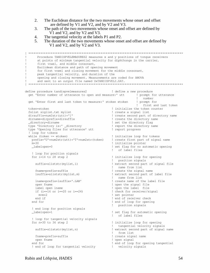
2. The Euclidean distance for the two movements whose onset and offset are defined by V1 and V2, and by V2 and V3.

3. The path of the two movements whose onset and offset are defined by V1 and V2, and by V2 and V3.

4. The tangential velocity at the labels P1 and P2.5. The duration of the two movements whose onset and offset are defined by

V1 and V2, and by V2 and V3.

! ******************************************************************************************! Procedure TANDISPVELEMASURES2 measures x and y positions of tongue receivers! at points of minimum tangential velocity for diphthongs in the carrier,! first vowel, and middle consonant,! Euclidean distance and path of opening movement! for first vowel and closing movement for the middle consonant,! peak tangential velocity, and duration of the! opening and closing movement. Measurements are coded for ANOVA! and sent to an output file named UxTANDISPVEL2.DAT.! ******************************************************************************************

define procedure tandispvelmeasures2 ! define a new procedure get "Enter number of utterance to open and measure:" utt ! prompt for utterance

! number get "Enter first and last token to measure:" stoken etoken ! prompt for

! first and last token token=stoken ! initialize the token counter fslist siglist.txt mylist ! create a signal list dirsuffix=num2str(utt)+"]" ! create second part of directory name dirname=dirprefix+dirsuffix ! create the directory name _directory=dirname ! set the directory flag type "Directory is:" _directory ! report the directory name type "Opening files for utterance" utt ! report progress ! loop for tokens while (token <= etoken) ! initialize loop for tokens prefix="U"+num2str(utt)+"T"+num2str(token) ! create first part of signal name m=30 ! initialize pointer _labelopen=0 ! set flag for no automatic opening

! of label files ! loop for position signals for i=14 to 28 step 2 ! initialize loop for opening

! position signals suffix=sliststr(mylist,i) ! extract second part of signal file

! name from list fname=prefix+suffix ! create the signal name lsuffix=sliststr(mylist,m) ! extract second part of label file

! name from list lname=prefix+lsuffix+".LAB" ! create name of the label file open fname ! open the signal file label open lname ! open the label file if (i==16 or i==20 or i==24) ! check for receiver/signal m=m+2 ! set pointer end if ! end of receiver check end for ! end of loop for opening

! position signals ! end loop for position signals _labelopen=1 ! set flag for automatic opening

! of label files ! loop for tangential velocity signals for n=30 to 36 step 2 ! initialize loop for opening

! tangential velocity signals suffix=sliststr(mylist,n) ! extract second part of signal name

! from list fname=prefix+suffix ! create signal name open fname ! open signal end for ! end of loop for opening tangential ! end of loop for tangential velocity ! velocity signals


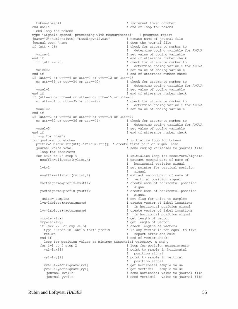
token=token+1 ! increment token counter end while ! end of loop for tokens ! end loop for tokens type "Signals opened, proceeding with measurements!" ! progress report jname="U"+num2str(utt)+"tandispvel2.dat" ! create name of journal file journal open jname ! open the journal file if (utt < 28) ! check for utterance number to

! determine coding variable for ANOVA voice=1 ! set value of coding variable end if ! end of utterance number check if (utt >= 28) ! check for utterance number to

! determine coding variable for ANOVA voice=2 ! set value of coding variable end if ! end of utterance number check if (utt==1 or utt==6 or utt==7 or utt==13 or utt==28 or utt==33 or utt==34 or utt==40) ! check for utterance number to

! determine coding variable for ANOVA vowel=1 ! set value of coding variable end if ! end of utterance number check if (utt==3 or utt==4 or utt==8 or utt==15 or utt==30 or utt==31 or utt==35 or utt==42) ! check for utterance number to

! determine coding variable for ANOVA vowel=2 ! set value of coding variable end if if (utt==2 or utt==5 or utt==9 or utt==14 or utt==29 or utt==32 or utt==36 or utt==41) ! check for utterance number to

! determine coding variable for ANOVA vowel=3 ! set value of coding variable end if ! end of utterance number check ! loop for tokens for j=stoken to etoken ! initialize loop for tokens prefix="U"+num2str(utt)+"T"+num2str(j) ! create first part of signal name journal voice vowel ! send coding variables to journal file ! loop for receivers for k=14 to 26 step 4 ! initialize loop for receivers/signals xsuffix=sliststr(mylist,k) ! extract second part of name of

! horizontal position signal l=k+2 ! set pointer for vertical position

! signal ysuffix=sliststr(mylist,l) ! extract second part of name of

! vertical position signal xactsigname=prefix+xsuffix ! create name of horizontal position

! signal yactsigname=prefix+ysuffix ! create name of horizontal position

! signal _units=_samples ! set flag for units to samples lvx=lablocs(xactsigname) ! create vector of label locations

! in horizontal position signal lvy=lablocs(yactsigname) ! create vector of label locations

! in horizontal position signal mxx=len(lvx) ! get length of vector mxy=len(lvy) ! get length of vector if (mxx <>5 or mxy <> 5) ! check lengths of vectors type "Error in labels for:" prefix ! if any vector is not equal to five return ! report error and exit end if ! end of vector check ! loop for position values at minimum tangential velocity, x and y for i=1 to 5 step 2 ! loop for position measurements vx1=lvx[i] ! point to sample in horizontal

! position signal vy1=lvy[i] ! point to sample in vertical

! position signal xvalue=xactsigname[vx1] ! get horizontal sample value yvalue=yactsigname[vy1] ! get vertical sample value

journal xvalue ! send horizontal value to journal file journal yvalue ! send vertical value to journal file


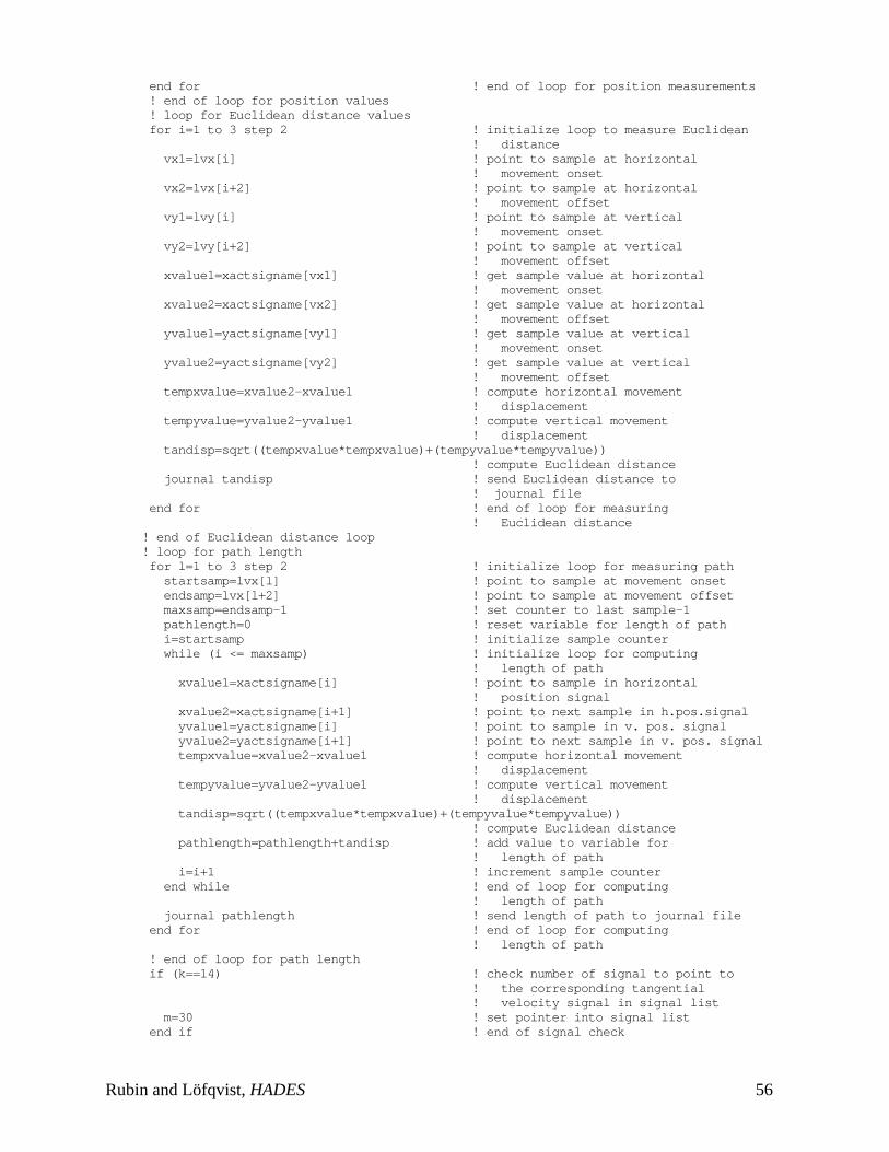
end for ! end of loop for position measurements ! end of loop for position values ! loop for Euclidean distance values for i=1 to 3 step 2 ! initialize loop to measure Euclidean

! distance vx1=lvx[i] ! point to sample at horizontal

! movement onset vx2=lvx[i+2] ! point to sample at horizontal

! movement offset vy1=lvy[i] ! point to sample at vertical

! movement onset vy2=lvy[i+2] ! point to sample at vertical

! movement offset xvalue1=xactsigname[vx1] ! get sample value at horizontal

! movement onset xvalue2=xactsigname[vx2] ! get sample value at horizontal

! movement offset yvalue1=yactsigname[vy1] ! get sample value at vertical

! movement onset yvalue2=yactsigname[vy2] ! get sample value at vertical

! movement offset tempxvalue=xvalue2-xvalue1 ! compute horizontal movement

! displacement tempyvalue=yvalue2-yvalue1 ! compute vertical movement

! displacement tandisp=sqrt((tempxvalue*tempxvalue)+(tempyvalue*tempyvalue))

! compute Euclidean distance journal tandisp ! send Euclidean distance to

! journal file end for ! end of loop for measuring

! Euclidean distance ! end of Euclidean distance loop ! loop for path length for l=1 to 3 step 2 ! initialize loop for measuring path startsamp=lvx[l] ! point to sample at movement onset endsamp=lvx[l+2] ! point to sample at movement offset maxsamp=endsamp-1 ! set counter to last sample-1 pathlength=0 ! reset variable for length of path i=startsamp ! initialize sample counter while (i <= maxsamp) ! initialize loop for computing

! length of path xvalue1=xactsigname[i] ! point to sample in horizontal

! position signal xvalue2=xactsigname[i+1] ! point to next sample in h.pos.signal yvalue1=yactsigname[i] ! point to sample in v. pos. signal yvalue2=yactsigname[i+1] ! point to next sample in v. pos. signal tempxvalue=xvalue2-xvalue1 ! compute horizontal movement

! displacement tempyvalue=yvalue2-yvalue1 ! compute vertical movement

! displacement tandisp=sqrt((tempxvalue*tempxvalue)+(tempyvalue*tempyvalue))

! compute Euclidean distance pathlength=pathlength+tandisp ! add value to variable for

! length of path i=i+1 ! increment sample counter end while ! end of loop for computing

! length of path journal pathlength ! send length of path to journal file end for ! end of loop for computing

! length of path ! end of loop for path length if (k==14) ! check number of signal to point to

! the corresponding tangential ! velocity signal in signal list

m=30 ! set pointer into signal list end if ! end of signal check


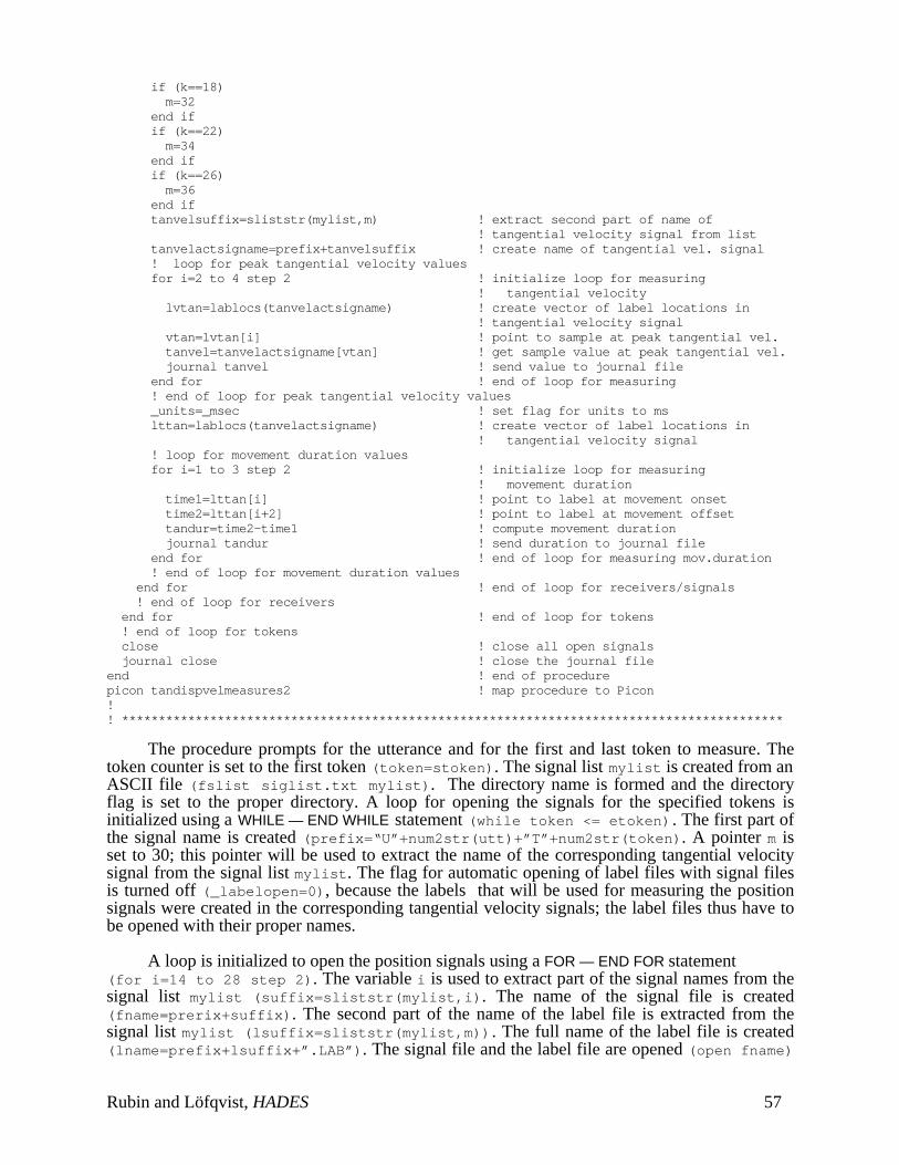
if (k==18) m=32 end if if (k==22) m=34 end if if (k==26) m=36 end if tanvelsuffix=sliststr(mylist,m) ! extract second part of name of

! tangential velocity signal from list tanvelactsigname=prefix+tanvelsuffix ! create name of tangential vel. signal ! loop for peak tangential velocity values for i=2 to 4 step 2 ! initialize loop for measuring

! tangential velocity lvtan=lablocs(tanvelactsigname) ! create vector of label locations in

! tangential velocity signal vtan=lvtan[i] ! point to sample at peak tangential vel. tanvel=tanvelactsigname[vtan] ! get sample value at peak tangential vel. journal tanvel ! send value to journal file end for ! end of loop for measuring ! end of loop for peak tangential velocity values _units=_msec ! set flag for units to ms lttan=lablocs(tanvelactsigname) ! create vector of label locations in

! tangential velocity signal ! loop for movement duration values for i=1 to 3 step 2 ! initialize loop for measuring

! movement duration time1=lttan[i] ! point to label at movement onset time2=lttan[i+2] ! point to label at movement offset tandur=time2-time1 ! compute movement duration journal tandur ! send duration to journal file end for ! end of loop for measuring mov.duration ! end of loop for movement duration values end for ! end of loop for receivers/signals ! end of loop for receivers end for ! end of loop for tokens ! end of loop for tokens close ! close all open signals journal close ! close the journal fileend ! end of procedurepicon tandispvelmeasures2 ! map procedure to Picon!! ******************************************************************************************

The procedure prompts for the utterance and for the first and last token to measure. Thetoken counter is set to the first token (token=stoken). The signal list mylist is created from anASCII file (fslist siglist.txt mylist). The directory name is formed and the directoryflag is set to the proper directory. A loop for opening the signals for the specified tokens isinitialized using a WHILE — END WHILE statement (while token <= etoken) . The first part ofthe signal name is created (prefix=“U”+num2str(utt)+”T”+num2str(token). A pointer m isset to 30; this pointer will be used to extract the name of the corresponding tangential velocitysignal from the signal list mylist. The flag for automatic opening of label files with signal filesis turned off (_labelopen=0), because the labels that will be used for measuring the positionsignals were created in the corresponding tangential velocity signals; the label files thus have tobe opened with their proper names.

A loop is initialized to open the position signals using a FOR — END FOR statement(for i=14 to 28 step 2). The variable i is used to extract part of the signal names from thesignal list mylist (suffix=sliststr(mylist,i). The name of the signal file is created(fname=prerix+suffix). The second part of the name of the label file is extracted from thesignal list mylist (lsuffix=sliststr(mylist,m)). The full name of the label file is created(lname=prefix+lsuffix+”.LAB”). The signal file and the label file are opened (open fname)


(label open lname). The receiver is checked and the pointer m is set to the proper value, i.e. ifthe next position signal to be opened is from the same receiver, the pointer remains unchanged,otherwise it is incremented. When all the position signals have been opened with the proper labelfiles, the flag for automatic opening of label files with signal files is turned on (_labelopen=1),since the tangential velocity signals will be opened with their own label files. A loop for openingthe tangential velocity signals is started using a FOR — END FOR statement (for n=30 to 36step 2). The second part of the signal name is extracted from the signal list, the complete nameis formed, and the signal is opened. The token counter is incremented (token=token+1) and theprocess is repeated until the signals for all the specified tokens have been opened and a progressreport is typed.

The name of a journal file into which the measurements will be saved is formed(jname=“U”+num2str(utt)+”tandispvel2.dat”) and the journal file is opened (journalopen jname). The number of the utterance being measured is evaluated in order to set twocoding variables (voice, vowel) that will be used later in an Analysis of Variance.

A loop for measuring the specified tokens is started using a FOR — END FOR statement(for j=stoken to etoken). The first part of the signal name is created and the codingvariables are sent to the journal file (journal voice vowel). A loop for receivers is initializedusing a FOR — END FOR statement (for k=14 to 26 step 4). The second part of the name ofthe horizontal position signal is extracted from the signal list (xsuffix=sliststr(mylist,k))and a pointer (l=k+2) is set to extract the second part of the name of the vertical position signal(ysuffix=sliststr(mylist,l)). The full names of the horizontal and vertical position signalsare created. The flag for units is set to samples (_units=_samples) since sample values will bemeasured. Two vectors of label positions are created for the horizontal(lvx=lablocs(xactsigname)) and vertical (lvy=lablocs(yactsigname) position signals,respectively. The length of the two vectors is calculated (mxx=len(lvx) and (mxy=len(lvy). Acheck is made to see if the length of any of the two vectors differs from 5 (if (mxx <5> ormxy <> 5)), in which case an error message is typed and the procedure stops.

A loop is started to get the horizontal and vertical positions at the labels V1, V2, and V3 inFigure IV.2, using a FOR — END FOR statement (for i=1 to 5 step 2). A pointer is set to thehorizontal and vertical sample (vx1=lvx[i]) (vy1=lvy[i]) and the sample values areobtained (xvalue=xactsigname[vx1]) and (yvalue=yactsigname[lvy1]. The values are sentto the journal file.

A new loop is created to calculate Euclidean distance as a measure of movementdisplacement using a FOR — END FOR statement (for i=1 to 3 step 2). To make thiscalculation, the horizontal and vertical receiver positions at movement onset and offset arerequired. Four pointers are set to the proper values: onset and offset in horizontal position(vx1=lvx[i]) and (vx2=lvx[i=2]) and onset and offset in vertical position (vy1[lvy[i]) and(vy2=lvy[i+2]). The sample values at these points are obtained, and the horizontal and verticalmovement displacements are calculated (tempxvalue=xvalue2-xvalue1) and(tempyvalue=yvalue2-yvalue1). Finally, the Euclidean distance is calculated(tandisp=sqr((tempxvalue*tempxvalue)+(temyvalue*tempyvalue)), and this value is sentto the journal file (journal tandisp).

Another loop is started to measure the path traversed by a receiver during a movement byadding the Euclidean distance between successive samples from movement onset to movementoffset (for l=1 to 3 step 2). The sample locations at movement onset and offset areobtained (startsamp=lvx[l]) and (endsamp=lvx[l+2]). A counter is set to the last sampleminus 1 (maxsamp=endsamp-1). A variable for the length of the path is set to zero(pathlength=0). A sample counter is set to the sample at movement onset (i=startsamp) anda loop is created using a WHILE — END WHILE statement (while (i = maxsamp)). Twopointers are set to the first and second samples in the horizontal position signal


(xvalue1=xactsigname[i]) and (xvalue2=xactsigname[i+1]) and two other pointers are setto the corresponding samples in the vertical position signal (yvalue1=yactsigname[i]) and(yvalue2=yactsigname[i+1]). The horizontal and vertical distance between these samples arecalculated (tempxvalue=xvalue2-xvalue1) and (tempyvalue=yvalue2-yvalue1), and thenthe Euclidean distance between the samples(tandisp=sqr((tempxvalue*tempxvalue)+(temyvalue*tempyvalue)).This value is added to the variable pathlength (pathlength=pathlength+tandisp).The sample counter is incremented (i=i+1), and the procedure repeated until all the sampleshave been processed.

A check is made of the number of the position signal to set a pointer to the correspondingtangential velocity signal in the signal list mylist. The second part of the name of the tangentialvelocity signal is extracted from the list and then the full name of the signal is created. A loop isinitialized to measure the tangential velocity at the labels P1 and P2 in Figure IV.2 (for i=2 to4 step 2). A vector of label positions in the tangential velocity signal is created(lvtan=lablocs(tanvelactsigname)). A pointer is set to the sample at the first label(lvtan=lvtan[i]), and the sample value is obtained (tanvel=tanvelactsigname[vtan]).This value is sent to the journal file (journal tanvel), and the loop is repeated.

To measure movement duration, the flag for units is set to ms (_units=_msec) and avector of label positions in the tangential velocity signal is created(lttan=lablocs(tanvelactsigname)). A loop is created for the measurements (for i=1 to3 step 2). Two pointers are set to the labels at movement onset and offset, respectively(time1=lttan[i]) and (time2=lttan[i+2]). The duration between movement onset andoffset is calculated (tandur=time2-time1) and the result is sent to the journal file (journaltandur). When all the measurements for the first receiver have been made, the receiver loop isrepeated until all receivers have been processed for the first token. Then, the token loop isincremented and the measurements for that token are made until all tokens have been processed.All open signals are closed (close *) and the journal file is closed (journal close).

The journal file with the results of the measurements can later be read by a statisticsprogram to obtain descriptive and inferential analyses of the data.


V. FUTURE DEVELOPMENTS

A third flavor of HADES, called MHADES, is presently under development. MHADESis designed for full compatability with the DECwindows / Motif user interface. This willprovide for a more intuitive design, because all HADES windows will use the same graphicalelements (widgets) that are used in the parent operating system. In addition, all of the displaycode is being redesigned to make the program more reliable. A potential future implication inmoving to Motif is the increased possibility of cross-platform HADES development,including the possibility of versions of HADES that run on UNIX-based systems, such as theSUN SPARCstation and the Silicon Graphics family of CPUs. These platforms are availableat Haskins for testing and development. Unfortunately, a considerable investment of effortwould need to be spent removing all system-specific code from HADES. In particular,HADES makes greate reliance on the VAX T$PARSE library of string parsing code and on aset of specialized, VAX-specific, low-level file input-output routines. At this point, cross-platform development of HADES is being evaluated.

Another flavor of HADES is in the planning stages. AHADES is a version of MHADESthat will run on Digital’s newer Alpha (DEC AXP) platform. MHADES is being developed ina manner that will permit easy porting to the Alpha environment. This will let users takeadvantage of the increased processing power of this RISC-based platform. We expect thatAHADES would become available within several months of the completion of MHADES.

At present, XHADES can be run from Macintosh computers attached to our Ethernetnetwork running an X Windows emulation program called eXodus, from White PineSoftware. Most of the graphics in the present paper were created by using the eXodusemulator and then capturing the screen displays. We have also tested remote connections toour network, using a the eXodus eXpress product via TCP/IP. This test has proven successful.eXodus eXpress also supports high speed serial/modem connections. The increasedthroughput of newer inexpensive modems (14,400 and 28,800 baud), and the availability ofISDN and other connectivity solutions, make this approach a promising way for individualsto run HADES from their home or university computers.

Another feature that we would like to add to MHADES is the enhanced animation ofpoint movement data, particularly to show EMMA receiver trajectories. We presently use theLissajous display to provide a limited view of such data. A separate program called MBAT(MicroBeam Analysis Tool) was developed at Haskins Laboratories by Mark Tiede toprovide for such animation. Tiede has moved to the ATR Human Information Laboratoriesand has developed an enhanced, Motif version of MBAT called MAVIS (Multiple ArticulatorVISualizer; Tiede, 1994). MAVIS is used for viewing synchronized movement data such asthat generated by point source tracking methods like the magnetometer or X-ray microbeamsystems. It provides simultaneous display of paired time-varying trajectories and their spatialdistribution at a temporal offset, which can be incremented automatically for powerfulanimation effects. The program also supports concurrent display of static backgrounds suchas a palate trace. We hope to provide some of this functionality within MHADES in the formof new midsagittal point animation window. This window will let the user have control overthe animation speed, the size and color of points, and will provide a VCR mode for replayinganimations and for easily moving back and forth through them.


VI. CONCLUSION

Desktop computers can now be used as affordable laboratory tools for analyzing speechand physiological signals. Examples include the PC-based CSRE system (Jamieson, et al,1989), and Signalyze (Keller, 1992) and SpeechTools (GW Instruments, 1992) for theMacintosh. The movement towards XWindows / Motif interfaces on engineering workstationsprovides the user-friendly graphical environment of the desktop computer coupled with theprocessing power and data throughput of these more powerful processors. A variety of suchsystems are available, including Waves for UNIX-based systems, the new N!Power by STI,and the HADES family of programs.

This paper has concentrated on HADES, detailing some of its most important features,including a wide variety of display and analysis tools. The most important feature of HADES,however, is its underlying procedural language, SPIEL. In part this language is similar to theprogram based scripting languages in applications such as Excel and Matlab. An importantdifference is that the focus of SPIEL is much narrower than in these other scriptinglanguages. SPIEL has been optimized to handle large data sets of time-varying physiologicaland audio signals. The emphasis of this system is in providing researchers with sets ofprimitives and tools, and a language to control them, that makes the job of displaying,manipulating, measuring and analyzing large data sets as simple as possible. The programincludes a variety of specialized tools (such as its rich event marking package), but omitsmany of the sophisticated analyses found in other signal processing packages. The intent ofHADES was to develop a package that focused on a set of specific approaches, but alsointegrated smoothly with other programs. The combination of the SPIEL procedurallanguage, the ability to label significant events in signals, facilities for journaling data inASCII files, and simple data import and export, provide this vehicle. HADES is rarely used inisolation. As can be seen in the example in the present paper, sophisticated analyses andmeasurement techniques can provide output to be used by other programs, such as statisticalpackages, spreadsheets, etc., without concern for the destination platform.

HADES continues to be used at a variety of institutions around the world. Althoughdevelopment of the system has slowed over the past year as the package has stabilized, wehope to continue modernizing it and making it easier to use with the many powerfulprograms available on both desktop computers and engineering workstations. Also exciting isthe beginning of the development of sophisticated procedures in the SPIEL language, as seenin the present paper. This ongoing development should prove extremely valuable for bothfine-tuning and extending the HADES system.


ACKNOWLEDGEMENTS

The HADES family of programs and the SPIEL procedural language were designed byPhilip Rubin — he is the one to blame should you be unhappy with any of the features of theprogram and its underlying language. The SPIEL procedure examples described in section IV ofthis paper were developed by Anders Löfqvist — contact him if you have any questions aboutthem.

The following individuals, in order, were the main programmers of the HADES system —Vance Maverick, Mark Tiede, Marian Pressler, and Simon Levy. Without their tireless effortsand strong opinions about the design and direction of the program, HADES would not exist.HADES has, in part, developed from earlier programs. A particular influence has been programsand tools developed by Lenny Szubowicz. Significant contributions were derived from the workof Richard McGowan and Douglas Whalen. Members of the Haskins programming staff andtechnical support staff have contributed in a variety of ways to this project. These individuals areMichael D’Angelo, Vincent Gulisano, William Scully, Donald Hailey and Ed Wiley. Theinstallation and tuning of the EMMA system, along with software for its use at HaskinsLaboratories has had a major impact upon the development of HADES. Thuse who contributed inthis area include Vincent Gracco, Anders Löfqvist , Patrick Nye, Michael D’Angelo, EricVatikiotis-Bateson, and Mark Tiede. Louis Goldstein provided design consultation on theSPEED prototpe. The design of the formant tracing package was influenced by suggestions fromRobert Remez, Jennifer Fellowes and Jennifer Pardo. We are also grateful to the IEEE for thedevelopment of their fine package of signal processing subroutines, to Seiichi Tenpaku and theATR Laboratories for the use of a portion of their SpeechTools package, to Eric Keller for hissupport of the Haskins PCM format in his Signalyze program, and to the many users of HADESwho, over the years, have provided valuable feedback and support. Thanks!

GRANT SUPPORT

The design and development of HADES has been supported, in part, by grants andcontracts from the National Institutes of Health to Haskins Laboratories including NIH GrantHD-01994, NIH-Grant DC-00121, NIH Grant DC-00043, NIH Grant DC-00044, NIH Grant DC-00825, NIH Grant DC-00865, NIH Contract N01-HD-5-2190, and support from the ATRLaboratories in Kyoto, Japan.

COPYRIGHT

HADES and SPIEL are (c) 1991, 1995, by Haskins Laboratories and Philip Rubin.


REFERENCES

Alfonso, Peter J., Neely, J. Robert, Van Lieshout, Pascal H. H. M., Hulstijn, Walter, and Peters,Herman F. M. (1993). Calibration, validation, and hardware-software modifications to theCarstens EMMA system. Forschungsberichte des Instituts für Phonetik und SprachlicheKommunikation der Universität München (FIPKM), 31, 105-120.

Atal, B. S. (1985). Linear predictive coding of speech. In F. Fallside & W. A. Woods (Eds.),Computer Speech Processing. Prentice-Hall, International.

Cyphers, D. S. (1985). Spire: A Research Tool. S. M. Thesis, Massachusetts Institute ofTechnology, Cambridge, MA.

Davenport, T. & Vellon, M. (1987). Tag Image File Format - Rev 4.0. Aldus/Microsoft TechnicalMemorandum, 4-31.

Fallside, F. (1985). Frequency-domain analysis of speech. In F. Fallside & W. A. Woods (Eds.),Computer Speech Processing. Prentice-Hall, International.

Fallside, Frank & Woods, William A. (Eds.). (1985). Computer Speech Processing. Prentice-Hall, International.

Gayvert, R. T., Biles, J. A., Rhody, H., and Hillenbrand, J. (1989). ESPRIT: A signal processingenvironment with a visual programming interface. Journal of the Acoustical Society ofAmerica, 85 (Supl), S57.

Gracco, Vincent L. & Nye, Patrick W. (1993). Magnetometry in speech articulation research:Some misadventures on the road to enlightenment. Forschungsberichte des Instituts fürPhonetik und Sprachliche Kommunikation der Universität München (FIPKM), 31, 91-104.

GW Instruments, Inc. (1992). SoundScope User’s Manual. Manual Version 1.0. GWI,Somerville, MA. September 15, 1992.

Henke, W. L. (1987). MITSYN Languages: A Coherent Family of High-Level Languages forTime Signal Processing. Language Reference Manual, V 6.0. Belmont, MA: WLH.

IEEE Acoustics, Speech, and Signal Processing Society. (1979). Programs for Digital SignalProcessing. New York: IEEE Press.

Jamieson, Donald G., Nearey, Terrance M. & Ramji, Ketan. (1989). CSRE: A Speech ResearchEnvironment. Canadian Acoustics / Acoustique canadienne, 17 (4), 23-35.

Keller, Eric. (1992). Signalyze. Signal Analysis for Speech and Sound. User’s Manual Version2.0, January 1992. InfoSignal, Inc., Lausanne, Switzerland.

Löfqvist, Anders & Gracco, Vincent L. (1994). Tongue body kinematics in velar stopproduction: Influences of consonant voicing and vowel context. Phonetica 51: 52-67.

Löfqvist, Anders, Gracco, Vincent L. & Nye, Patrick W. (1993). Recording Speech MovementsUsing Magnetometry: One Laboratory’s Experience. Forschungsberichte des Instituts fürPhonetik und Sprachliche Kommunikation der Universität München (FIPKM), 31, 143-162.


Markel, J. & Gray, A. (1976). Linear Prediction of Speech. Springer-Verlag, New York.

Maverick, Vance and Rubin, Philip. (1988). SPEED — Signal Processing, Editing and Display.Internal Haskins Laboratories documentation note, November, 1988.

O’Shaughnessy, D. (1987). Speech Communication: Human and Machine. Addison-Wesley,Reading, MA.

O’Shaughnessy, D. (1995). Speech technology. In R. Bennett, S. L. Greenspan & A. Syrdal(Eds.), Behavioral Aspects of Speech Technology: Theory and Applications. Elsevier.

Perkell, J., Cohen, M., Svirsky, M., Matthies, M., Garabieta, I. & Jackson, M. (1992).Electromagnetic midsagittal articulomter (EMMA) systems for transducing speecharticulatory movements. Journal of the Acoustical Society of America, 92, 3078-3096.

Rabiner, L. R. and Schafer, R. W. (1979). Digital Processing of Speech Signals. Prentice Hall,Englewood Cliffs, New Jersey.

Remez, R. E., Rubin, P. E., Pisoni, D. B., & Carrell, T. D. (1981). Speech perception withouttraditional speech cues. Science, 212, 947-950.

Remez, R.E., Rubin, P. E., Berns, S. M., Pardo, J. S. & Lang, J. M. (1994). On the perceptualorganization of speech. Psychological Review, 101, 129-156.

Rubin, P. E. (1980). Sinewave synthesis. Internal memorandum. Haskins Laboratories, NewHaven, CT

Rubin, Philip E. (1995). HADES: A Case Study of the Development of a Signal AnalysisSystem. In R. Bennett, S. L. Greenspan & A. Syrdal (Eds.), Behavioral Aspects ofSpeech Technology: Theory and Applications. Elsevier.

Rubin, P., MacEachron, M., Tiede, M., and Maverick, V. (1991). Haskins Analysis, Display, andExperiment System (HADES). Haskins Laboratories Internal Memorandu, October,1991. Haskins Laboratories, New Haven, CT

Strum, R. D. and Kirk, D. D. (1989). First Principles of Discrete Systems and Digital SignalProcessing. Addison-Wesley, Reading, MA.

Szubowicz, L. S. (1982). WENDY Version 1.6 Reference Manual. Haskins Laboratories internaldocumentation note.

Tenpaku, Seiichi. (1992). SpeechTools. Internal memorandum. ATR Research Laboratories,Kyoto, Japan.

The MathWorks, Inc. (1991). MATLAB User’s Guide. The MathWorks, Inc., Natick, MA.

Tiede, Mark. (1994). MAVIS. Multiple articulator visualization. Internal memorandum. ATRHuman Information Laboratories, Kyoto, Japan.

Vatikiotis-Bateson, E. , Hirayama, M., Wada, Y. and Kawato, M. (1993).Generating articulator motion from muscle activity using artificial neural networks.Ann. Bull. RILP (Tokyo University), 27, 67-77.


Vatikiotis-Bateson , E. and Kelso, J. A. S. (1993). Rhythm type and articulatory dynamics inEnglish, Japanese and French. Journal of Phonetics, 21, 231-265

Wada, Y., Koike, Vatikiotis-Bateson, E., and Kawato, M. (in press). A computational theory formovement pattern recognition based on optimal movement pattern generation.Biological Cybernetics.

Whalen, D. H., Wiley, E. R., Rubin, P. E., & Cooper, F. S. (1990). The Haskins Laboratories'pulse code modulation (PCM) system. Behavior Research Methods, Instruments, &Computers, 22, 550-59.

Witten, Ian H. (1982). Principles of Computer Speech. Academic Press, Inc., London.

Zue, V. W., Cyphers, D. S., Kassel, R. H., Kaufman, D. H., Leung, H. C., Randolph, M., Seneff,S., Unverferth, J. E. III, and Wilson, T. (1986). The development of the MIT LISP-Machine based speech research workstation. Proceedings of the ICASSP 86,International Conference on Acoustics, Speech, and Signal Processing, held in Tokyo,Japan, April 8-11, 329-332.


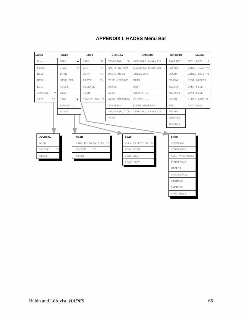
APPENDIX I: HADES Menu Bar

FLAGS

JOURNAL ➢

About ...

HELP

NEWS

EDIT

QUIT ^Z

PLAY ➢

LIST

OPEN ➢

SAVE

SAVE SEL

CLOSE

SHOW ➢

CUT ^K

TRIM

UNDO ^U

COPY ^R

PASTE ^V

SILENCE

SELECT ALL ^A

HADES DATA EDIT DISPLAY PROCESS EFFECTS LABEL

SIGNAL ...

SLIST

OPEN

JOURNAL

ON/OFF ^Z

CLOSE

SAMPLED DATA FILE ^F

OPEN

ON/OFF ^Z

CLOSE

COMMANDS

SHOW

CONSTANTS

FLAG VARIABLES

EMPTY WINDOW

LISS

TEMPORAL ^D

PHOTO MODE

TILE WINDOWS

PHASE

AXIS DEFAULTS

3D-SPECT

CROSS-SECTION

SPECTRAL SNAPSHOT

SMOOTH...

SPECTRAL ANALYSIS...

INTEGRATE

MEAN

RMS

FILTER...

CENTER

FADEOUT

AMPLIFY

DCADD

DEMEAN

FADEIN

FLOOR

FULL

INVERT

LABEL HEAD ^H

SAVE FILE

SET LABEL ^L

LABEL TAIL ^T

LIST LABELS

OPEN FILE

CLEAR LABELS

AUTOLABEL

TIFF RECTIFY

REVERSE

EVENT MARKING

TEMPORAL ANALYSIS

PLAY SELECTION ^P

PLAY

PLAY VIEW

PLAY ALL

PLAY LAST FUNCTIONS

MACROS

PROCEDURES

SIGNALS

SYMBOLS

VARIABLES


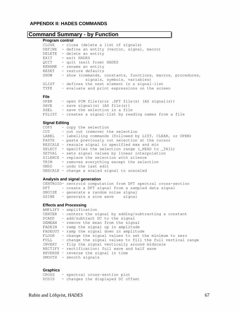
APPENDIX II: HADES COMMANDS

Command Summary - by FunctionProgram controlCLOSE - close (delete a list of signals)DEFINE - define an entity (vector, signal, macro)DELETE - delete an entityEXIT - exit HADESQUIT - quit (exit from) HADESRENAME - rename an entityRESET - restore defaultsSHOW - show (commands, constants, functions, macros, procedures,

signals, symbols, variables)SLIST - defines the next element in a signal-listTYPE - evaluate and print expressions on the screen

FileOPEN - open PCM file(s)or .DFT file(s) (AS signal(s))SAVE - save signal(s) (AS file(s))SSEL - save the selection in a fileFSLIST - creates a signal-list by reading names from a file

Signal EditingCOPY - copy the selectionCUT - cut out (remove) the selectionLABEL - labelling commands (followed by LIST, CLEAR, or OPEN)PASTE - paste previously cut selection at the cursorRESCALE - rescale signal to specified max and minSELECT - specifies the selection range (_HEAD to _TAIL)SETVAL - sets signal values by linear interpolationSILENCE - replace the selection with silenceTRIM - removes everything except the selectionUNDO - undo the last editUNSCALE - change a scaled signal to unscaled

Analysis and signal generationCENTROID- centroid computation from DFT spectral cross-sectionDFT - create a DFT signal from a sampled data signalGNOISE - generate a random noise signalGSINE - generate a sine wave signal

Effects and ProcessingAMPLIFY - amplificationCENTER - centers the signal by adding/subtracting a constantDCADD - add/subtract DC to the signalDEMEAN - remove the mean from the signalFADEIN - ramp the signal up in amplitudeFADEOUT - ramp the signal down in amplitudeFLOOR - change the signal values to set the minimum to zeroFULL - change the signal values to fill the full vertical rangeINVERT - flip the signal vertically around midscaleRECTIFY - rectification: full wave and half waveREVERSE - reverse the signal in timeSMOOTH - smooth signals

GraphicsCROSS - spectral cross-section plotDCDIS - changes the displayed DC offset


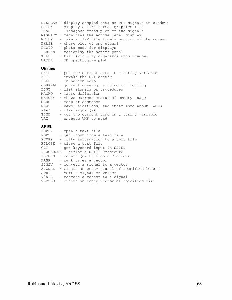
DISPLAY - display sampled data or DFT signals in windowsDTIFF - display a TIFF-format graphics fileLISS - lissajous cross-plot of two signalsMAGNIFY - magnifies the active panel displayMTIFF - make a TIFF file from a portion of the screenPHASE - phase plot of one signalPHOTO - photo mode for displaysREDRAW - redisplay the active panelTILE - tile (visually organize) open windowsWATER - 3D spectrogram plot

UtilitiesDATE - put the current date in a string variableEDIT - invoke the EDT editorHELP - on-screen helpJOURNAL - journal opening, writing or togglingLIST - list signals or proceduresMACRO - macro definitionMEMORY - shows current status of memory usageMENU - menu of commandsNEWS - news, additions, and other info about HADESPLAY - play signal(s)TIME - put the current time in a string variableVAX - execute VMS command

SPIELFOPEN - open a text fileFGET - get input from a text fileFTYPE - write information to a text fileFCLOSE - close a text fileGET - get keyboard input in SPIELPROCEDURE - define a SPIEL ProcedureRETURN - return (exit) from a ProcedureRANK - rank order a vectorSIG2V - convert a signal to a vectorSIGNAL - create an empty signal of specified lengthSORT - sort a signal or vectorV2SIG - convert a vector to a signalVECTOR - create an empty vector of specified size


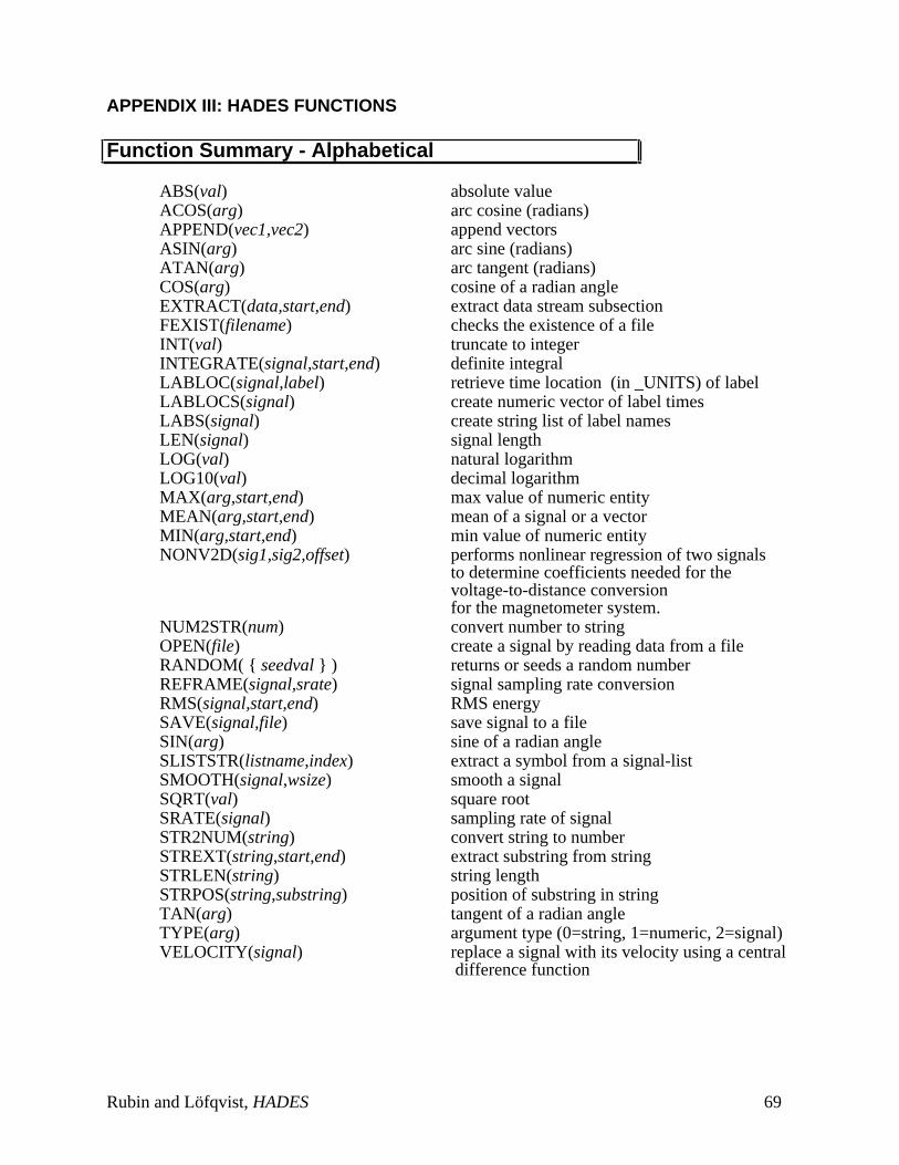
APPENDIX III: HADES FUNCTIONS

Function Summary - Alphabetical

ABS(val) absolute valueACOS(arg) arc cosine (radians)APPEND(vec1,vec2) append vectorsASIN(arg) arc sine (radians)ATAN(arg) arc tangent (radians)COS(arg) cosine of a radian angleEXTRACT(data,start,end) extract data stream subsectionFEXIST(filename) checks the existence of a fileINT(val) truncate to integerINTEGRATE(signal,start,end) definite integralLABLOC(signal,label) retrieve time location (in _UNITS) of labelLABLOCS(signal) create numeric vector of label timesLABS(signal) create string list of label namesLEN(signal) signal lengthLOG(val) natural logarithmLOG10(val) decimal logarithmMAX(arg,start,end) max value of numeric entityMEAN(arg,start,end) mean of a signal or a vectorMIN(arg,start,end) min value of numeric entityNONV2D(sig1,sig2,offset) performs nonlinear regression of two signals

to determine coefficients needed for thevoltage-to-distance conversionfor the magnetometer system.

NUM2STR(num) convert number to stringOPEN(file) create a signal by reading data from a fileRANDOM( { seedval } ) returns or seeds a random numberREFRAME(signal,srate) signal sampling rate conversionRMS(signal,start,end) RMS energySAVE(signal,file) save signal to a fileSIN(arg) sine of a radian angleSLISTSTR(listname,index) extract a symbol from a signal-listSMOOTH(signal,wsize) smooth a signalSQRT(val) square rootSRATE(signal) sampling rate of signalSTR2NUM(string) convert string to numberSTREXT(string,start,end) extract substring from stringSTRLEN(string) string lengthSTRPOS(string,substring) position of substring in stringTAN(arg) tangent of a radian angleTYPE(arg) argument type (0=string, 1=numeric, 2=signal)VELOCITY(signal) replace a signal with its velocity using a central

difference function


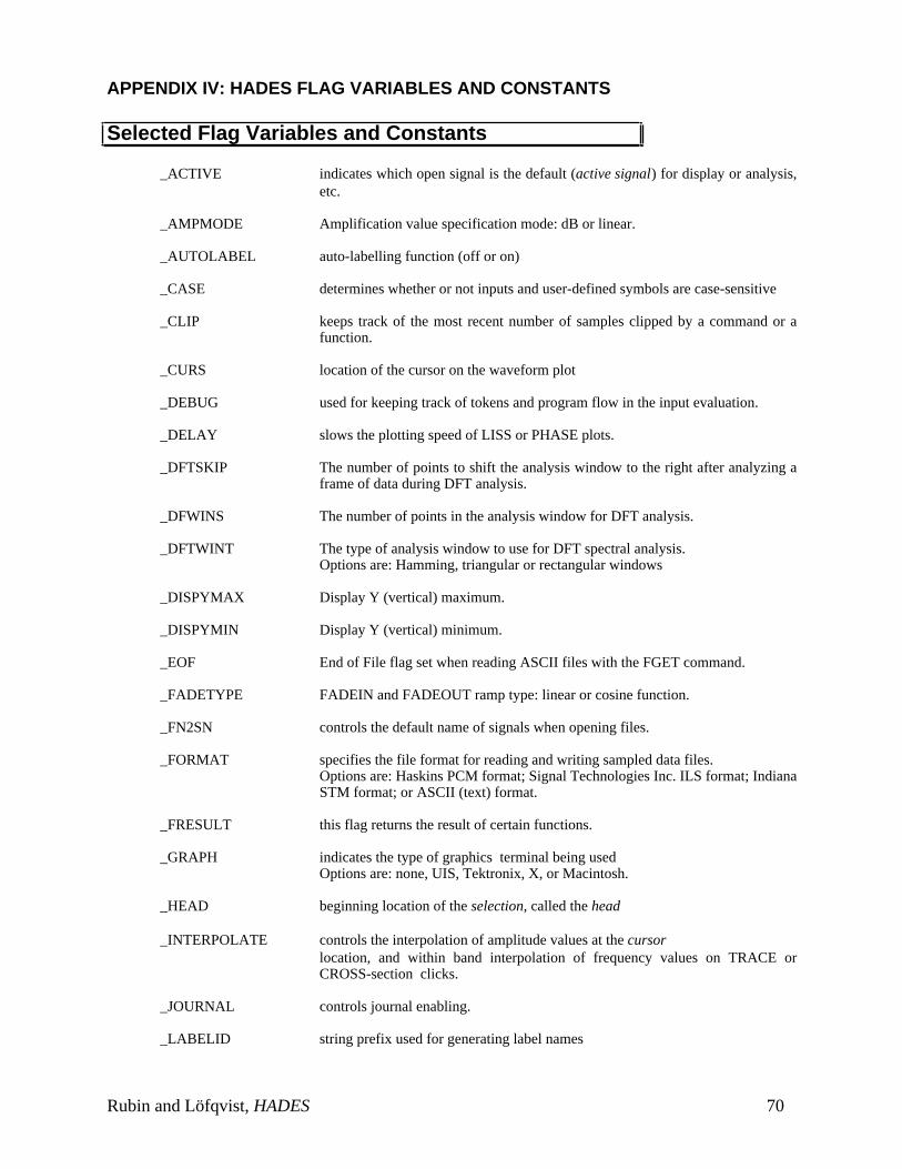
APPENDIX IV: HADES FLAG VARIABLES AND CONSTANTS

Selected Flag Variables and Constants

_ACTIVE indicates which open signal is the default (active signal) for display or analysis,etc.

_AMPMODE Amplification value specification mode: dB or linear.

_AUTOLABEL auto-labelling function (off or on)

_CASE determines whether or not inputs and user-defined symbols are case-sensitive

_CLIP keeps track of the most recent number of samples clipped by a command or afunction.

_CURS location of the cursor on the waveform plot

_DEBUG used for keeping track of tokens and program flow in the input evaluation.

_DELAY slows the plotting speed of LISS or PHASE plots.

_DFTSKIP The number of points to shift the analysis window to the right after analyzing aframe of data during DFT analysis.

_DFWINS The number of points in the analysis window for DFT analysis.

_DFTWINT The type of analysis window to use for DFT spectral analysis.Options are: Hamming, triangular or rectangular windows

_DISPYMAX Display Y (vertical) maximum.

_DISPYMIN Display Y (vertical) minimum.

_EOF End of File flag set when reading ASCII files with the FGET command.

_FADETYPE FADEIN and FADEOUT ramp type: linear or cosine function.

_FN2SN controls the default name of signals when opening files.

_FORMAT specifies the file format for reading and writing sampled data files.Options are: Haskins PCM format; Signal Technologies Inc. ILS format; IndianaSTM format; or ASCII (text) format.

_FRESULT this flag returns the result of certain functions.

_GRAPH indicates the type of graphics terminal being usedOptions are: none, UIS, Tektronix, X, or Macintosh.

_HEAD beginning location of the selection, called the head

_INTERPOLATE controls the interpolation of amplitude values at the cursorlocation, and within band interpolation of frequency values on TRACE orCROSS-section clicks.

_JOURNAL controls journal enabling.

_LABELID string prefix used for generating label names


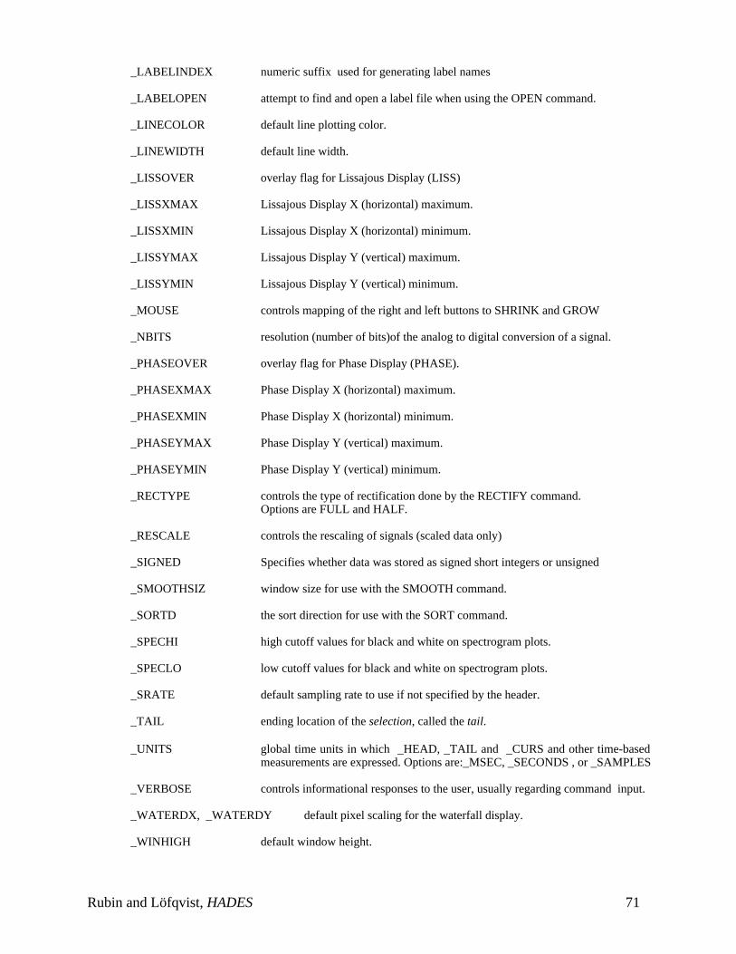
_LABELINDEX numeric suffix used for generating label names

_LABELOPEN attempt to find and open a label file when using the OPEN command.

_LINECOLOR default line plotting color.

_LINEWIDTH default line width.

_LISSOVER overlay flag for Lissajous Display (LISS)

_LISSXMAX Lissajous Display X (horizontal) maximum.

_LISSXMIN Lissajous Display X (horizontal) minimum.

_LISSYMAX Lissajous Display Y (vertical) maximum.

_LISSYMIN Lissajous Display Y (vertical) minimum.

_MOUSE controls mapping of the right and left buttons to SHRINK and GROW

_NBITS resolution (number of bits)of the analog to digital conversion of a signal.

_PHASEOVER overlay flag for Phase Display (PHASE).

_PHASEXMAX Phase Display X (horizontal) maximum.

_PHASEXMIN Phase Display X (horizontal) minimum.

_PHASEYMAX Phase Display Y (vertical) maximum.

_PHASEYMIN Phase Display Y (vertical) minimum.

_RECTYPE controls the type of rectification done by the RECTIFY command.Options are FULL and HALF.

_RESCALE controls the rescaling of signals (scaled data only)

_SIGNED Specifies whether data was stored as signed short integers or unsigned

_SMOOTHSIZ window size for use with the SMOOTH command.

_SORTD the sort direction for use with the SORT command.

_SPECHI high cutoff values for black and white on spectrogram plots.

_SPECLO low cutoff values for black and white on spectrogram plots.

_SRATE default sampling rate to use if not specified by the header.

_TAIL ending location of the selection, called the tail.

_UNITS global time units in which _HEAD, _TAIL and _CURS and other time-basedmeasurements are expressed. Options are:_MSEC, _SECONDS , or _SAMPLES

_VERBOSE controls informational responses to the user, usually regarding command input.

_WATERDX, _WATERDY default pixel scaling for the waterfall display.

_WINHIGH default window height.


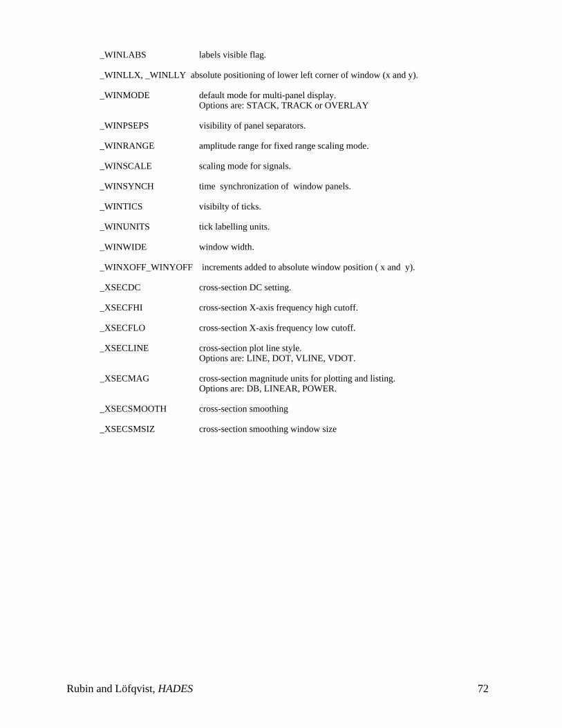
_WINLABS labels visible flag.

_WINLLX, _WINLLY absolute positioning of lower left corner of window (x and y).

_WINMODE default mode for multi-panel display.Options are: STACK, TRACK or OVERLAY

_WINPSEPS visibility of panel separators.

_WINRANGE amplitude range for fixed range scaling mode.

_WINSCALE scaling mode for signals.

_WINSYNCH time synchronization of window panels.

_WINTICS visibilty of ticks.

_WINUNITS tick labelling units.

_WINWIDE window width.

_WINXOFF_WINYOFF increments added to absolute window position ( x and y).

_XSECDC cross-section DC setting.

_XSECFHI cross-section X-axis frequency high cutoff.

_XSECFLO cross-section X-axis frequency low cutoff.

_XSECLINE cross-section plot line style.Options are: LINE, DOT, VLINE, VDOT.

_XSECMAG cross-section magnitude units for plotting and listing.Options are: DB, LINEAR, POWER.

_XSECSMOOTH cross-section smoothing

_XSECSMSIZ cross-section smoothing window size


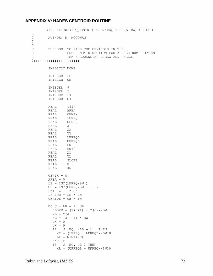
APPENDIX V: HADES CENTROID ROUTINE

SUBROUTINE SPA_CENTX ( Y, LFREQ, UFREQ, BW, CENTX )CC AUTHOR: R. MCGOWANCCC PURPOSE: TO FIND THE CENTROID IN THEC FREQUENCY DIRECTION FOR A SPECTRUM BETWEENC THE FREQUENCIES LFREQ AND UFREQ.C::::::::::::::::::::::

IMPLICIT NONE

INTEGER LB INTEGER UB

INTEGER J INTEGER I INTEGER LX INTEGER UX

REAL Y(1) REAL AREA REAL CENTX REAL LFREQ REAL UFREQ REAL X REAL XX REAL YY REAL LFREQB REAL UFREQB REAL BW REAL BW10 REAL XL REAL YL REAL SLOPE REAL H REAL XR

CENTX = 0. AREA = 0. LB = INT(LFREQ/BW ) UB = INT(UFREQ/BW + 1. ) BW10 = .1 * BW LFREQB = LB * BW UFREQB = UB * BW

DO J = LB + 1, UB SLOPE = (Y(J+1) - Y(J))/BW YL = Y(J) XL = (J - 1) * BW LX = 0 UX = 9 IF ( J .EQ. (LB + 1)) THEN XR = (LFREQ - LFREQB)/BW10 LX = NINT(XR) END IF IF ( J .EQ. UB ) THEN XR = (UFREQB - UFREQ)/BW10


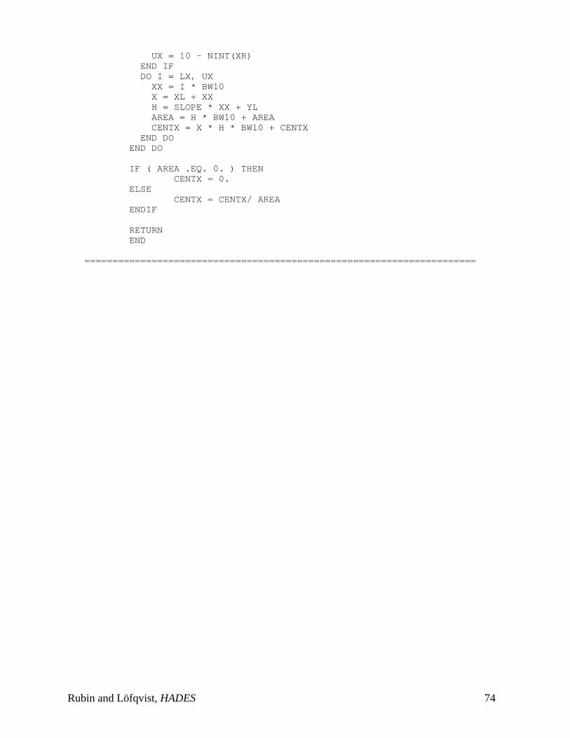
UX = 10 - NINT(XR) END IF DO I = LX, UX XX = I * BW10 X = XL + XX H = SLOPE * XX + YL AREA = H * BW10 + AREA CENTX = X * H * BW10 + CENTX END DO END DO

IF ( AREA .EQ. 0. ) THEN CENTX = 0. ELSE CENTX = CENTX/ AREA ENDIF

RETURN END

======================================================================


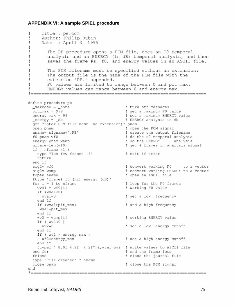
APPENDIX VI: A sample SPIEL procedure

! Title : pe.com! Author: Philip Rubin! Date : April 3, 1995!! The PE procedure opens a PCM file, does an F0 temporal! analysis and an ENERGY (in dB) temporal analysis, and then! saves the frame #s, f0, and energy values in an ASCII file.!! The PCM filename must be specified without an extension.! The output file is the name of the PCM file with the! extension "PE." appended.! F0 values are limited to range between 0 and pit_max.! ENERGY values can range between 0 and energy_max.!=================================================================

define procedure pe _verbose = _none ! turn off messages pit_max = 999 ! set a maximum F0 value energy_max = 99 ! set a maximum ENERGY value _energy = _db ! ENERGY analysis in db get "Enter PCM file name (no extension)" pnam open pnam ! open the PCM signal aname=_signame+".PE" ! create the output filename f0 pnam wf0 ! do the F0 temporal analysis energy pnam wamp ! do the ENERGY analysis nframe=len(wf0) ! get # frames in analysis signal if ( nframe <1 ) type "Too few frames !!" ! exit if error return end if sig2v wf0 ! convert working F0 to a vector sig2v wamp ! convert working ENERGY to a vector fopen aname ! open an ASCII file ftype "frame# f0 (Hz) energy (dB)" for i = 1 to nframe ! loop for the F0 frames wval = wf0[i] ! working F0 value if (wval<0) wval=0 ! set a low frequency end if if (wval>pit_max) ! and a high frequency wval=pit_max end if wv2 = wamp[i] ! working ENERGY value if ( wv2<0 ) wv2=0 ! set a low energy cutoff end if if ( wv2 > energy_max ) wf2=energy_max ! set a high energy cutoff end if ftypef " %.0f %.2f %.2f",i,wval,wv2 ! write values to ASCII file end for ! end the frame loop fclose ! close the journal file type "File created: " aname close pnam ! close the PCM signalend!=================================================================


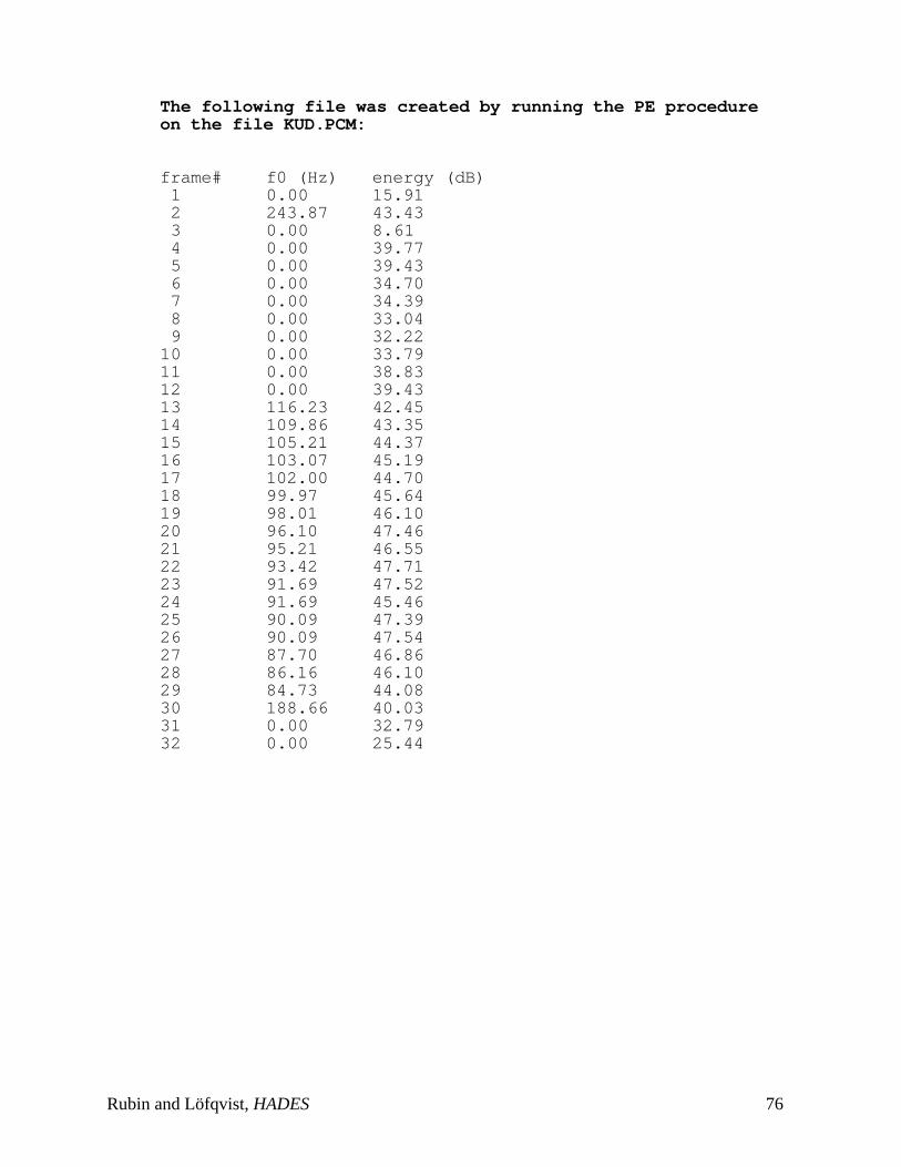
The following file was created by running the PE procedureon the file KUD.PCM:

frame# f0 (Hz) energy (dB) 1 0.00 15.91

2 243.87 43.43 3 0.00 8.61 4 0.00 39.77 5 0.00 39.43 6 0.00 34.70 7 0.00 34.39 8 0.00 33.04 9 0.00 32.22

10 0.00 33.79 11 0.00 38.83 12 0.00 39.43 13 116.23 42.45 14 109.86 43.35

15 105.21 44.37 16 103.07 45.19 17 102.00 44.70 18 99.97 45.64 19 98.01 46.10 20 96.10 47.46 21 95.21 46.55

22 93.42 47.7123 91.69 47.52

24 91.69 45.4625 90.09 47.3926 90.09 47.54

27 87.70 46.86 28 86.16 46.10 29 84.73 44.08 30 188.66 40.03

31 0.00 32.79 32 0.00 25.44


FIGURE CAPTIONS:

Figure 1: HADES GUI, showing menu bar and command window

Figure 2: HADES Menu Bar

Figure 3: Analysis Parameters Dialog Box

Figure 4: Panel Toolbox Dialog Box

Figure 5: The Display Window

Figure 6: PICON: The Programmable Icon

Figure 7: HADES Display Window

Figure 8: The Control Panel

Figure 9: Display Window with waveform and spectrogram

Figure 10: Spectral cross-section

Figure 11: 3D Waterfall spectral display

Figure 12: Multi-panel Display Window

Figure 13: Multi-panel display window — overlayed

Figure 14: Lissajous display

Figure 15: Phase display

Figure 16: TIFF display of MRI of vocal tract

Figure 17: Display Window showing a labelled signal

Figure 18: A hand-labelled signal

Figure 19: A signal labelled by means of autolabelling

Figure 20: Event Marking dialog box

Figure 21: Filter Parameters dialog box

Figure 22: DFT, LPC, and FBA display

Figure 23: The Temporal Analysis Parameters Dialog Box

Figure 24: The Flags Dialog Box

Figure 25: The Axis Settings Dialog Box


Figure 26: Example of a window created using the procedure tandisplay.The signals are from top to bottom, audio, tangential velocity of tongue tip, tongue blade, tongue body, and tongue root.

Figure 27: The same display as in Figure 26 with labels in the tangential velocitysignals

Appendix I: HADES Menu Bar


HADES - Haskins Laboratories · sound systems, which can be ... HADES , called MHADES , ... each...

Documents

Transcript of HADES - Haskins Laboratories · sound systems, which can be ... HADES , called MHADES , ... each...