Biological Services ProgramandDivision of Ecological Services

r.. :~ ~ ;: ~ ~~y

t...... .:, . !: ~ V;';;th nds Research CenterU. ' : _~ . F L-: ~ ,'-l;"1d '~n ldhfe Servi ce'i" ,~ . .~ C i ~ j 'd Z"l ~lo rac BoulevardL';'{.lydle. La. 70506

FWS/OBS·82/10.16JULY 1982

HABITAT SUITABILITY INDEX MODELS:LARGEMOUTH BASS

. . " . . . .~ . " . : ..'

Fish and Wildlife Service

S. Department of the InteriorSK36 1. U54no. 82 ­10. 16

The Biological Services Program was establi shed wi t hin t he U.S. Fishand Wildlife Service to supply scientific information and me thodologies onkey environmental issues that impact fish and wi l dli fe reso urces and theirsupporting ecosystems. The mission of the program is as follows:

• To strengthen the Fish and Wi l dl i fe Se rv i ce in its role asa primary source of information on national f ish and wild­life reso urces, particularly i n respect to environmentalimpact assessment. .

• To gather, analyze, and present info rmation that wi l l ai ddecisionmakers in the identi fication and resolut ion ofproblems associated with maj or changes in land and wateruse.

• To provide bet ter ecolog ical i nformation and eval uat ionfor Department of the Interior development programs , suchas those rel at i ng to energy developme nt.

Informat ion develo ped by the Biologi cal Ser vic es Program is i nt endedfor use i n the planni ng and decis ionma ki ng process to prevent or mi nimi zethe impact of devel opment on fi sh and ~I il d li fe . Research activ ities andtechnical assistance services are based on an analysis of t he is sues , adetermina tion of t he decisionma kers involved and the i r i nformati on needs,and an evaluat ion of t he st ate of t he ar t to identi fy i nformat ion ~aps

and to determine priorit ies. This i s a st ra tegy that wi l l ensur e t hatthe product s produced and di sseminated are t ime ly and useful .

Proj ects ' have been initi ated i n the foll owing areas : coal ext ract ionand convers ion; power pl ants ; geothermal , mineral and oil shal e develop­men t; water res ource analysis , j ncludi ng s tream alterations and west er nwater al location ; coastal ecosystems and Ou te r Con tinent al Shel f devel op­ment ; and systems inventory , incl uding Nati onal Wetl and Inventory,habita t clas si f i cation and analysi s, and informat i on t ransfe r .

The Bi ological Servi ces Program consists of the Offi ce of Biol ogi calSer vi ces in Washingto n, D.C . , wh i ch i s r esponsib l e for overal l planning andma nagement; Nat ional Teams, whi ch provide the Program's cent ra l scie nti fi cand technical expertise and arrange ~o r contract i ng bi ol09ica l services Istudies with states, universit ie s, consulting firms , and others; Reg iona lSta f fs , who provide a link t o problems at t he operati ng leve l; and staffs atcertain Fish and Wil dli fe Ser vice resear ch facili t i es , wh o conduct i n-houseresearch studies .

FWS/OBS-82/10.16July 1982

HABITAT SUITABILITY INDEX MODELS: LARGEMOUTH BASS

by

Robert J. StuberHabitat Evaluation Procedures GroupWestern Energy and Land Use Team

U.S. Fish and Wildlife ServiceDrake Creekside Building One

2625 Redwing RoadFort Collins, CO 80526

Glen Gebhartand

O. Eugene MaughanOklahoma Cooperative Fishery Research Unit

Oklahoma State UniversityStillwater, OK 74074

Western Energy and Land Use TeamOffice of Biological Services

Fish and Wildlife ServiceU.S. Department of the Interior

Washington, DC 20240

This report should be cited as:

Stuber, R. J., G. Gebhart, and O. E. Maughan. 1982. Habitat suitabilityindex models: Largemouth bass. U.S. Dept. Int. Fish Wildl. ServoFWS/OBS-82/10.16. 32 pp.

PREFACE

The habitat use information and Habitat Suitability Index (HSI) modelspresented in this document are an aid for impact assessment and habitat manaae­ment activities. Literature concerning a species' habitat requirements andpreferences is reviewed and then synthesized into HSI models, which are scaledto produce an index between 0 (unsuitable habitat) and 1 (optimal habitat).Assumptions used to transform habitat use information into these mathematicalmodels are noted, and guidelines for model application are described. Anymodels found in the literature which can also be used to calculate an HSI are.cited, and simplified HSI models, based on what the authors believe to be themost important characteristics for this species, are presented.

Use of the models presented in this publication for impact assessmentrequires the setting of clear study objectives and may require modification ofthe models to meet those objectives. Methods for reducing model complexityand recommended measurement techniques for model variables are presented inTerrell et al. (in press).l A discussion of HSI model building techniques,including the component approach, is presented in U.S. Fish and WildlifeService (1981).2

The HSI models presented herein are complex hypotheses of species-habitatrelationships, not statements of proven cause and effect relationships.Results of modelPerformance tests, when available, are referenced; however,models that have demonstrated reliability in specific situations may proveunreliable in others. For this reason, the U.S. Fish and Wildlife Serviceencourages model users to send comments and suggestions that might help usincrease the utility and effectiveness of this habitat-based approach to fishand wildlife planning. Please send comments to:

Habitat Evaluation Procedures GroupWestern Energy and Land Use TeamU.S. Fish and Wildlife Service2625 Redwing RoadFt. Collins, CO 80526

lTerrell, J. W., T. E. McMahon, P. D. In s ki p , R. F. Raleigh, and K. W.Williamson (-in press). Habitat Suitability Index Models: Appendix A.Guidelines for riverine and lacustrine applications of fish HSI modelswith the habitat evaluation procedures. U.S. Dept. Int. Fish Wildl.Servo FWS/OBS 82-10.A.

2U.S. Fish and Wildlife Service. 1981. Standards for the development ofHabitat Suitability Index models. 103 ESM. U.S. Dept. Int. Fish Wildl.Serv., Div. Ecol. Servo

CONTENTS

Page

PREFACE iiiACKNOWLEDGMENTS v

HABITAT USE INFORMATION 1Genera 1 •.•...•.•..•.•.•...•...•••••••••.••••••...••••••••••.•••••• 1Age t Growth t and Food 1Reproduct ion 1Specifi c Habitat Requi rements 2

HABITAT SUITABILITY INDEX (HSI) MODELS 4Model Applicability 4Model Description - Riverine...................................... 5Model Description - Lacustrine... 5Suitability Index (SI) Graphs for Model Variables 8Riverine Model 16Lacustrine Model 17Interpreting Model Outputs........................................ 22

ADDITIONAL HABITAT MODELS 22Mode 1 1 22Model 2 27Model 3 27

REFERENCES

iv

27

ACKNOWLEDGMENTS

We would like to thank James Clugston, George Elliot, Jim Winter, WilliamReynolds, Martha Casterlin, Robert Summerfelt, and Richard Anderson for review­ing the manuscript. Their review contributions are gratefully acknowledged,but the authors accept full responsibility for the contents of the document.Word processing was provided by Dora Ibarra and Carolyn Gulzow. Coverillustration is from Freshwater Fishes of Canada, Bulletin 184, FisheriesResearch Board of Canada, by W. B. Scott and E. J. Crossman.

v

LARGEMOUTH BASS (Micropterus salm~iges)

HABITAT USE INFORMATION

General

The largemouth bass (Mi~!..Q£teru~ salmoides) is native to the easternUnited States, excluding the Northeastern States (MacCrimmon and Robbins1975), and has been introduced throughout the United States (Robbins andMacCrimmon 1974). Two subspecies are recognized, the northern subspecies, M.salmoides salmoides, and the Florida subspecies, M. salmoides floridan~s(BiliTey-and~ubbs 1949; Hart 1952; Ramsey 1975). ---------

Age, Growth, and Food

The maximum known age of largemouth bass is 15 years, and the normal rateof growth for adult largemouth is approximately 454 g per year (Bennett 1937;Anderson 1975). Largemouth bass mature and spawn as early as age I near thesouthern limit of their range (Morgan 1958; Clugston 1964; La Faunce et a1.1964; Smitherman 1975). Maturity is delayed among more northern populations(Eipper and Regier 1962; Bennett 1971; Carlander 1977). In Canada, maturityis reached in 3-4 years for males and 4-5 years for females (Scott and Crossman1973) .

l.ar-qernout.h bass fry feed mainly on microcrustaceans and small insects,juveniles consume mostly insects and small fish, and adults feed primarily onfish and crayfish (Emig 1966; Zweiacker and Summerfe1t 1974; Car1ander 1977).Adults often feed near vegetation within shallow areas. Largemouth bassfeeding intensity is bimodal, with peaks in the early morning and late evening(Snow 1971; Olmstead 1974).

Reproduction

Spawning typically begins in the spring when the water temperature reaches12.0-15.5° C (Mraz 1964; Miller and Kramer 1971). Spawning has been recordedbetween 11.5 and 29.0° C, but most occurs between 16 and 22° C (Kramer andSmith 1960; Badenhuizen 1969; Carlson and Hale 1972). Incubation time rangesfrom 2 to 7 days, dependi ng on water temperature (Kramer and Smi th 1960;Badenhuizen 1969). The Florida subspecies nests and spawns earlier than thenorthern subspecies and at a 1 to 3° C lower temperature (Bottroff 1967).

A gravel substrate is preferred for spawning (Newell 1960; Robinson 1961;Mraz 1964), but largemouth bass will nest on a wide variety of other

1

substrates, including vegetation, roots, sand, mud, and cobble (Harlan andSpeak.er 1956; Mraz and Cooper 1957; Mraz et al. 1961). Nests are constructedby the male at water depths averaging 0.3-0.9 m, with depths ranging fromabout 0.15 m to 7.5 m (Swingle and Smith 1950; Harlan and Speaker 1956; Mraz1964; Clugston 1966; Allan and Romero 1975). Nests have been found as deep as8.23 m in a reservoir where depth increased during the spawning period (Millerand Kramer 1971).

Specific Habitat Requirements

Lacustri ne envi ronments are the preferred habi tat of 1argemouth bass(Emig 1966; Scott and Crossman 1973). Optimal conditions are lakes withextensive (~25% of surface area) shallow (~6 m depth) areas to supportsubmergent vegetation, yet deep enough (3-15 m mean depth) to successfullyoverwinter bass (Robbins and MacCrimmon 1974; Carlander 1977; Winter 1977).Thus, it is assumed that 40-60% of the lake area should be > 6 m depth toprovide optimal overwintering habitat in northern latitudes.

Optimal riverine habitat for largemouth bass is characterized by large.slow moving rivers or pools of streams with soft bottoms, some aquatic vege­tation, and relatively clear water (Trautman 1957; Larimore and Smith 1963;Scott and Crossman 1973). First and second order streams are generally poorhabi tat (Anderson, personal communicat ion). Deacon (1961) reported thatlargemouth bass abundance increased in rivers during dry years when the flowwas reduced and the water pooled. Thus, it is assumed that a ri ver wi th ahigh percent (~ 60%) of pool and backwater area is optimal. Also, largemouthbass prefer low gradient (s 1 m/km) streams; abundance decl ines as gradientincreases toward headwater areas (Finnell et al. 1956; Trautman 1957; Moyleand Nichols 1973). It is assumed that gradients> 4 m/km would be unsuitable.

Growth of largemouth bass is reduced at dissolved oxygen levels < 8 mg/l,and a sub stant i a 1 reduction occurs below 4 mg/l (Stewart et a 1. 1967).Distress may be evident at 5 mg/l (Katz et al. 1959; Whitmore et al. 1960;Dahlberg et al. 1968; Petit 1973). Levels below 1.0 mg/l are consideredlethal (Moss and Scott 1961; Mohler 1966; Petit 1973).

Standing crops of black basses (Micropterus spp.) are positively corre­lated with total dissolved solid levels of 100-350 ppm (Jenkins 1976).

Largemouth bass are considered intolerant of suspended solids (turbidity)and sediment (Muncy et a l . 1979). High levels of suspended solids may inter­fere with reproductive processes and reduce growth. Bulkley (1975) felt thathigh levels of suspended solids reduced the available food for largemouth bassto the extent that growth of maturing fish was reduced enough that they werephysically incapable of reproduction. Buck (1956a; 1956b) found that thegreatest survival and growth of largemouth bass occurred in ponds with tur­bidities (suspended solids) < 25 ppm. Growth was intermediate in ponds with25-100 ppm turbidity levels and lowest in ponds with turbidities> lUO ppm.Also, no young-of-the-year bass were found in the ponds with high turbidities,while they were recovered from the ponds with low and intermediate turbidities.Thus, optimum suspended solid levels are assumed to be 5-,25 ppm, and levels< 5 ppm indicate low productivity.

2

largemouth bass require a pH between 5 and 10 for successful reproduction(Swingle 1956; Buck and Thoits 1970). Using Stroud's (1967) criteria forfreshwater fish, optimal pH range is 6.5-8.5. largemouth bass can tolerateshort term exposures to pH levels of 3.9 and 10.5 (Calabrese 1969).

Adult. Adult largemouth bass are most abundant in areas with vegetation(Jenk.,..-nset al. 1952; Miller 1975) and ether forms of cover (e.g., logs,brush, and debri s ) . Optimal cover corresponds to 40-60~~ of the pool orlittoral area; too much cover may reduce prey availability (Saik.i and Tash1979). Adults are most abundant in areas of low current ve 1oc i ty , based oncatch data of Kallemyn and Novotny (1977) from the Missouri River. Optimalcurrent velocities are s 6 em/sec, and velocities> 20 em/sec are unsuitablebased on probability of use curves developed by Hardin and Bovee (1978).Increased water levels in reservoirs may reduce prey availability due toincreased cover for prey species. Stable to decreased water levels concen­trated prey, which increased feeding and growth rates of adult bass (Heman etal. 1969). Thus , stable to slightly negative midsummer fluctuations (0-3m)are considered optimal for adult largemouth bass.

Optimal temperatures for growth of adult bass range from 24-30° C (Mohler1966; Coutant 1975; Brungs and Jones 1977; Carlander 1977; Venables et al.1978). Very little growth occurs below 15° C (Mohler 1966) or above 36° C(Carlander 1977). Salinity levels above 4 ppt cause sharp declines in abundanceTebo and McCoy 1964). Kilby (1955) found no bass in Mississippi River coastalmarshes with salinities above 11.8 ppt, whereas Bailey et al. (1954) reportedfinding adult largemouth in water with salinities as high as 24.4 ppt in theEscambia River, Alabama and Florida.

Embryo. Optimal spawning substrate is gravel (Newell 1960; Robinson1961), but other substrates, such as vegetation, roots, sand, and mud, aresuitable (Harlan and Speaker 1956; Mraz and Cooper 1957; Mraz etal. 1961).Silty, muck.y bottoms are unsuitable (Robinson 1961). Exposed, shallow water« 1.5 m) nests are vulnerable to destruction by wave action (Miller andKramer 1971). Boulders, irregular bottoms, and other forms of shelter mayprotect these nests. Water velocities as low as 40 em/sec may result inmortality of embryos (Dudley 1969), and Hardin and Bovee (1978) reported thatvelocities> 10 em/sec were avoided by the species. Stable water levelsduring spawning are optimal; drawdowns often result in poor survival (Jesteret al. 1969). Since largemouth bass spawn at depths ranging from 0.15 m to7.5 m, it is assumed that drawdowns > 7.5 m are unsuitable for successfulembryonic development during spawning.

Optimal temperatures for successful spawning and incubation are 20-21° C(Clugston 1966; Badenhuizen 1969), with a range of 13-26° C (Carr 1942; Kelley1968). Survival is very low at temperatures> 30° C (Strawn 1961; Kelley1968; Badenhuizen 1969; McCormick and Wegner 1981) and < 10° C (Kramer andSmith 1960). Survival of embryos is impaired at salinities> 1.5 ppt, andzero at levels> 10.5 ppt (Tebo and McCoy 1964).

Fry. Optimal current velocities for fry are < 4 em/sec (Hardin and Bovee1978), and fry cannot tolerate current ve loci ties > 27 em/sec (Macleod 1967;laurence 1972). Cover, in the form of flooded terrestrial vegetation, is an

3

important requirement for fry habitat suitability, because the amount of coverhas been positively correlated to number of fry (Aggus and Elliot 1975).However, too much cover constitutes poor spawning habitat (R. O. Anderson,personal communication). Thus, it is assumed that optimal pools or littoralareas contain 40-80% cover. Also, stable to increased summer water level isoptimal, because it increases cover availability. It is assumed that decreas­ing (> 1 m) water levels would be suboptimal because fry would be more suscep­tible to predation with the decrease in available cover.

Optimal temperatures for fry growth are 27-30° C. Little growth occursbelow 15° C or above 32° C (Strawn 1961). The growth rate of fry declined atsalinities> 1.66 ppt and was zero at 6 ppt (Tebo and McCoy 1964).

Juvenile. Specific habitat requirements of juveniles are presumed to besimilar to those of adult largemouth bass.

HABITAT SUITABILITY INDEX (HSI) MODELS

Model Applicability

Geographic area. The models provided are applicable throughout the 48conterminous States. The standard of comparison for each individual variablesuitability index is the optimal value of the variable that occurs anywherewithin this region. Therefore, the models will never provide an HSI of 1.0when appl ied to northern waters where temperature related variables do notreach the optimal values found in the southern United States.

Season. The models provide a rating for a body of water based on itsabil ity to support a reproducing population of largemouth bass through allseasons of the year.

Cover types. The models are applicable in riverine, lacustrine, pal­ustrine, and estuarine habitats, as described by Cowardin et al. (1979).

Minimum habitat area. Minimum habitat area is defined as the minimumarea of contiguous suitable habitat that is required for a species to live andreproduce. No attempt has been made to establish a minimum habitat size forlargemouth bass.

Verification level. The acceptable output for each of these largemouthbass models is an index between 0 and 1 which the author believes has apositive relationship to carrying capacity. In order to verify that the modeloutput is acceptable, the author developed sample data sets from which HSI'swere calculated. These sample data sets and their relationship to modelverification will be discussed in greater detail following presentation of themode 1.

4

Model Description - Riverine

The structure of the riverine HSI model is depicted graphically inFi gure 1.

Food component. Percent bottom cover (V 3 , V4 ) is assumed to be important

because bottom cover provides habitat for aquatic insects, crayfish, andforage fish, which are the predominant food items of largemouth bass. Percentpool and backwater area (V 1 ) is included to quantify the amount of food

habitat.

Cover component. Percent bottom cover (V 3 , V4 ) is included because

larg'emouth bass are most abundant in areas with cover. Percent pool andbackwater area (V 1 ) quantifies the amount of cover habitat. Water level

fluctuation (V 1 6 , V1 S ) is assumed to be important because the amount of avail­

able cover is dependent on fluctuations.

Water quality component. The water quality component is limited todissolved oxygen (V 6 ) , pH range (V 7 ), temperature (Vs , VlD ), turbidity (V 1 1 ) ,

and salinity (V 1 2 , V1 3 ) measurements. These parameters have been shown to

affect growth or survival. Variables related to temperature and oxygen areassumed to be limiting when they reach near lethal levels. Toxic substancesare not considered in this model.

Reproductive component. Temperature (V 9 ) and salinity (V 1 4 ) during

spawning and embryonic deve l opmen t describe water quality conditions whichaffect reproduction. Maximum water level fluctuation (V 1 7 ) is included because

optimal development and survival is dependent on stable water levels duringspawning. Current velocity (V 2 0 ) is important because embryos require areas

of little or no velocity. Percent pool and backwater area (V 1 ) quantifies the

amount of low velocity spawning areas.

Other component. The variables which are in the other component arethose which also describe habitat suitability for the largemouth bass, yet arenot specifically related to the life requisite components already presented.Stream gradient (V 2 2 ) is included because largemouth bass prefer slow moving

streams. Current velocity (V 1 9 , V21 ) is an alternative way of describing the

habitat suitability of a riverine environment, because of the positive rela­tionship between gradient and current velocity.

Model Description - Lacustrine

Lacustrine model structure is depicted graphically in Figure 2.

5

Habitat Variables Life Requisite

Current velocity (V 1" Other

Stream gradient (Vz z )

pH range (V 7) ~~~===~~§§i§~.': Water qual fty (CWO) ------i HSITemperature (VI' V10)

Turbidity (V ll )

Salinity (V 12, V1J)

Current velocity (V20)

Dissolved oxygen

Water level fluctuation

Salinity (V 1.. )

Substrate (V lI )

% pool and backwater area (Vd~

% bottom cover (VJ, V.. ) --------------- Cover

Water level fluctuation (V 16, V1I)

% pool and backwater area (V1/)_--========::==~_ - Food (C F)% pool bottom cover (V J, V.. )-

% pool and backwater

Temperature (V'~)~==============::::~~~,.~ Reproduction (C R)

Figure 1. Tree diagram illustrating conceptual structure of riverinemodel for largemouth bass.

6

Habitat Variables Life Requisite

Total dissolved solids (VI) --------- Food (CF)

pH range (V 7).~~~========~~~§§§~w: Water qual ity (CwQ) --4 HSI

Water level fluctuation

Turbidity (V ll )

Temperature (VI. V1 0 )

Water level flucuation (V 1 6 •

Dissolved oxygen

% area S 6m deep (V2 )

Temperature (V'~)~==============~~~~~~~Salinity (V 1 . ) : Reproduction (C R)

Substrate (V 15 )

% area S 6m deep (V2 ) -------% bottom cover (V 2 • V.)

Figure 2. Tree diagram illustrating conceptual structure of lacustrinemodel for largemouth bass.

7

Food component. Average TDS (V s ) is included because there is a positive

correlation between standing crops of black. bass and TDS levels, presumablydue to the greater amount of food organisms produced at higher TDS levels.

Cover component. Percent bottom cover (V 3 , V4 ) is included because

largemouth bass are most abundant in areas with cover. Percent lacustrinearea ~ 6 m depth (V2 ) quantifies the amount of cover habitat. It also serves

to quantify the amount of overwintering habitat in northern latitudes. Waterlevel fluctuation (V 16 , V18 ) is assumed to be important because the amount of

available cover is dependent on fluctuations.

Water quality component. Same explanation as presented in the riverinemodel description.

Reproduction component. Temperature (V9 ) and salinity (V I 4 ) for spawning

and embryonic development describe water quality conditions which affectreproduction. Substrate (VIS) is important for spawning success. Water level

fluctuation (VI 7 ) is included because optimal development and survival of

embryos is dependent on stable water levels during spawning. Percentlacustrine area ~ 6 m depth (V2 ) quantifies the amount of spawning habitat.

Suitability Index (51) Graphs for Model Variables

This section contains suitability index graphs for the 22 variablesdescribed above and equations for combining selected variable indices into aspecies HSI using the component approach. The "R" and IILII refer to riverineand lacustrine habitat variables, respectively.

Habitat

R

Variable

Percent pool and back.­water area duringaverage summer flow.

8

L Vz Percent lacustrine 1.0area ~ 6 m depth. \ B

x \

Note: A regional con- ~ 0.8 \

sideration ~ sl:: A\..... \

made for bodies ~ 0.6 \

of water\

in more .....\

southern lati- .....0.4

\

tudes whereLJ \ttl~

overwintering .....~

requirements Vl 0.2are notas rigorous. 0.0

A. Northern lati- 0 25 50 75 100tudes

B. Southern lati- °L,0

tudes

R,L Vl Percent bottom cover 1.(e. g. , aquatic vegeta-tion, logs, and debris) x

QJ 0.8withi n pools, back- ~l::

waters, or 1i ttora 1 .....areas during summer. ~ 0.6(Adult, Juvenile) .....

.....LJ 0.4ttl.jJ

~

0.2Vl

0.00 25 50 75 100

%

R,L V4 Percent bottom cover 1.0(e. g, aquatic vegeta- xtion, logs, and debris) QJ

0.8within pools, back- ~l::

or littoral.....

waters,areas during

>,summer. ~ 0.6

( Fry)LJ 0.4ttl.jJ.....~

Vl 0.2

0.00 25 50 75 100

%

9

L Average TDS concentra­tion during growingseason when carbonate­bicarbonate> sulfate­chloride ionic concen­tration. If sulfate­chloride concentrationexceeds carbonate­bicarbonate, reduce SIrating for TDS by 0.2.

1.0xQ)

"0 0.8t::....~

+-> 0.6.r-r-.r-..cttl 0.4+->

.r-::sVl 0.2

O.O-+--_.............-.-......,,---......--r-+-

I

l-

I-

R,L Vb Minimum disssolved 1.0oxygen levels during xmidsummer within pools Q)

0.8"0or 1ittoral areas. t::....A) Frequently < 2 mg/T ~ 0.6.....B) Usually ~ 2 and r-

< 5 mg/l ..c 0.4ttlC) Usually ~ 5 and +->.....

< 8 mg/l ::s

D) Often > 8 mg/lVl 0.2

0.0

o 250

A B

500

ppm

C

750 1000

o

pH range during grow­ing season.

R,L V7

A)B)

C)

< 5.0 or > 10.0~ 5 and < 6.5 or> 8.5 and ~ 10-:06.5-8.5

1.0xQ)

0.8"0t::....~

+-> 0.6.....r-.......c 0.4ttl+->.....::sVl 0.2

0.0

-

-- I-

10

A B C

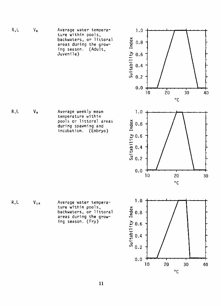
R,L VB Average water tempera- 1.0ture within pools,backwaters, or 1ittora 1 x

(1) 0.8areas during the grow- "0s::::

ing season. (Adult, .....Juvenile) ~ 0.6...............

oD 0.4s::l

0.2V'l

0.010 20 30 40

°C

R,L Vg Average weekly mean 1.0temperature withinpools or littoral areas x

(1) 0.8during spawning and "0s::::

incubation. (Embryo) .....~ 0.6..........~ 0.4+..l.....::l 0.2V'l

0.0 ...10 20 30

°C

R,L VlO Average water tempera- 1.0ture within pools, x

(1)

backwaters, or littoral -g 0.8areas during the grow- .....ing season. ( Fry) >,

+..l 0.6..........oD~ 0.4.....::l

V'l0.2

0.0 L10 20 30 40

°C

11

R,L Maximum monthly averageturbidity (suspendedsolids) during growingseason.

A) 5-25 ppmB) > 25 and ~ 100 ppmC) < 5 ppm, > lOG ppm

1.0XQJ

-g 0.8......>..~ 0.6r­.......0

Z:l 0.4......;:,

V)

0.2

- ~

-

0.0A B r:

"

R,L V12 Maximum salinity 1.0during summer.(Adult, Juvenile) x

~ 0.8s::......

~0.6......r-......~ 0.4~......;:,

V) 0.2

0.0a 6 12 18 24

ppt

R,L Vu Maximum sa 1in ity 1.0during summer.( Fry) x

QJ

'"C 0.8s::......

~0.6......r-......~ 0.4~......;:,

V) 0.2

0.0a 3 6

ppt

12

R,L Maximum sa l t ni tyduring spawning andincubation. (Embryo)

1.0xQ)

-g 0.8......>,

.;: 0.6

.....

.0s 0.4::::3

Vl 0.2

0.0a 3 6 9 12

ppt

R,L V15 Substrate composition 1.0within riverine poolsand backwaters or x

lacustrine littoral ~ 0.8c:

areas. (Embryo) ......

~O.6

A) Boulders and bed-rock predominate .....

~ 0.4(~ 50?~) +-'

B) Sand (0.062-2.0 mm) .....::::3

predominates Vl 0.2C) Silt and clay

(0.0-0.004 mm) 0.0predominate

D) Gravel (0.2-6.4 cm)predominates

I I

l

ABC 0

Average water levelfluctuation duringgrowing season.(Adult, Juvenile)

13

1.0xQ)

-g 0.8......>,~ 0.6

.0

.e 0.4::::3Vl

0.2

0.0-5 -2.5 a

m

2.5 5

R,L V17 Maximum water level 1.0fluctuation during xspawning. ( Embryo) Q)

-g 0.8......>,~ 0.6.....oD~ 0.4.....:::3

(/') 0.2

0.0-10 -5 0 5 10

m

R,L V18 Average water level 1.0fluctuation duringgrowing season. x

Q) 0.8( Fry) "0t:......

t' 0.6..........oD 0.4ttl+->.....:::3 0.2(/')

0.0-5 -2.5 0

m

R Vu Average current veloc- 1.0ity at 0.6 depthduring summer. x

Q)

0.8(Adult, Juvenile) "0t:......>,

+-> 0.6..........oD 0.4ttl+->.....:::3

(/') 0.2

0.00 5 10 15 20

em/sec

14

R V2Q Maximum current veloc- 1.0ity at 0.8 depth withinpools or backwaters )(

QJ 0.8during spawning (May- -0c

June). ( Embryo) ......

~ 0.6.~

.-

.~

.0 0.4I'tI

"""".~

~

VI 0.2

0.00 5.0 10.0

em/sec

R V2 ; Average current veloc- 1.0ity at 0.6 depth

)(during summer. ( Fry)~ 0.8c......

~ 0.6 L-e--.-.~

~ 0.4"""".~

~

VI 0.2

0.00 1.0 2.0 3.0

em/sec

R V22 Stream gradient withinrepresentative reach. 1.0

)(QJ-g 0.8

......>,

.4-J 0.6-e--

.~

~ 0.4"""".~

~

VI 0.2

0.00 1 2 3 4

m/km

15

Riverine Model

These equations utilize the life requisite approach and consist of fivecomponents: food, cover, water quality, reproduction, and other.

x

Cover (CC).

x

Water Quality (CWQ)'

If V1 2 and VI] = 1.0,

2V 6 + V7 + 2V. + V1 0 + VIICWQ = 7

If V1 2 or V < 1.0,

2V 6 + V7 + 2V. + VIa + VII +

CWQ = 8

If V6 , V., or VIa ~ 0.4, CWQ equals the lowest of the following:

V6 , V., VIa, or the above equation.

16

Reproduction (C ).R

If V1 4 = 1.0,

If V1 4 < 1.0,

Other (COT)'

Note: Since there is a correlation between stream gradient and currentvelocity, the user has two options for the "ot her" component:

A)2

, or

B) COT = v.,HSI determination.

If CWQ or CR is ~ 0.4, then the HSI equals the lowest of the

following: CWQ' CR or the above equation.

Lacustrine Model

These equations utilize the life requisite approach and consist of fourcomponents: food, cover, water quality, and reproduction.

17

Food (CF) .

CF = Vs

Cover (CC) .

Cc = [ V,(VJ + V4 ) r4

x 2 x V1 6 X V18

Water Quality (CWQ).

Same as the riverine habitat suitability index equations for waterquality.

Reproduction (CR).

If V14 = 1.0,

If V14 < 1.0,

HSI determination.

HSI = (CF x Cc x CWQ x CR)1/4

If CWQ or CR is S 0.4, then the HSI equals the lowest of the

following: CWQ; CR; or the above equation.

Sources of data and assumptions made in developing the suitability indicesare presented in Table 1.

18

Table 1. Data sources and assumptions for largemouth bass suitability indices.

Variabie and source

Trautman 1957Deacon 1961Larimore and Smith 1963Branson 1967Scott and Crossman 1973Funk 1975

Robbins and MacCrimmon 1974Carlander 1977\4i nter 1977

V3 Jenkins et al. 1952Miller 1975Saik.i and Tash 1979

V,. Kramer and Smith 1960Newell 1960Aggus and Elliot 1975Anderson 1981

Vs Jenkins 1976

Katz et al. 1959Whitmore et al. 1960Moss and Scott 1961Mohler 1966Stewart et al. 1967Dahlberg et al. 1968Petit 1973

~~~~~~e1~~~6(FW)aCalabrese 1969Buck. and Thoits 1970

Assumption

Largemouth bass typically inhabit pooland backwater areas of streams;optimal habitat consists of at least60% pool/backwater area.

Cover adequate to support large popula­tions can be provided by greater than25% area ~ 6 m depth. However,lacustrine habitats in northern latitudesneed to be deep enough to successfullyoverwinter bass.

Adult largemouth bass are most abundantin areas which contain cover; too muchcover may reduce prey availability.

The amount of cover has been positivelycorrelated with the number of fry. Toomuch cover constitutes poor spawningand rearing habitat.

Total dissolved solids (TDS) levelscorrelated with high standing crops areoptimal; those correlated with lowerstanding crops are suboptimal. Thedata used to develop this curve areprimarily from southeastern reservoirs.

Dissolved oxygen levels where growth isnot impaired are optimal, those wheregrowth is reduced are suboptimal, andthose where death may occur are unsuit­able.

Optimal pH range is presumably the sameas those for all freshwater fish. Levelswhich impair growth of largemouth bass aresuboptimal; those which can result indeath are unsuitable.

19

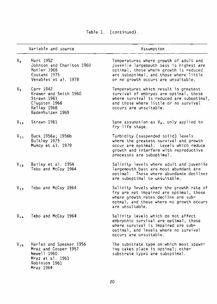
Table 1. (continued).

Variable and source

Va Hart 1952Johnson and Charlton 1960Mohler 1966Coutant 1975Venables et al. 1978

Vg Carr 1942Kramer and Smith 1960Strawn 1961Clugston 1966Ke 11 ey 1968Badenhuizen 1969

VlO Strawn 1961

Vll Buck 1956a; 1956bBulkley 1975Muncy et a1. 1979

Ba i 1ey et a1. 1954Tebo and McCoy 1964

Tebo and McCoy 1964

Tebo and McCoy 1964

Harlan and Speaker 1956Mraz and Cooper 1957Newell 1960Mraz at al. 1961Robinson 1961Mraz 1964

Assumption

Temperatures where growth of adult andjuveniie largemouth bass is highest areoptimal, those where growth is reducedare suboptimal. and those where littleor no growth occurs are unsuitable.

Temperatures which result in greatestsurvival of embryos are optimal, thosewhere survival is reduced are suboptimal,and those where little or no survivaloccurs are unsuitable.

Same assumption as Vg • only applied tofry life stage.

Turbidity (suspended solid) levelswhere the greatest survival and growthoccur are optimal. Levels which reducegrowth and interfere with reproductiveprocesses are suboptimal.

Salinity levels where adult and juvenilelargemouth bass are most abundant areoptimal. Those where abundance declinesare suboptimal to unsuitable.

Salinity levels where the growth rate offry are not impaired are optimal, thosewhere growth rates decline are sub­optmal. and those where no growth occursare unsuitable.

Salinity levels which do not affectembryonic survival are optimal, thosewhere survival is impaired are sub­optimal. and levels where no survivaloccurs are unsuitable.

The substrate type on which most spawn­ing takes place is optimal; othersubstrate types are suboptimal.

20

Table 1. (concluded).

Variable and source Assumption

V1 6 Heman et al. 1969

V1 7 Harlan and Speaker 1956Mraz 1964Clugston 1966Jester et al. 1969Allan a~d Romero 1975

VIS Aggus and Elliot 1975

VI <3 Sail ey et a1. 1954Kallemeyn and Novotny 1977Hardin and Bovee 1978

V2 0 Deacon 1961Dudley 1969

V2 1 Macleod 1967laurence 1972Hardin and Bovee 1978

V2 2 Finnell et al. 1956Trautman 1957Moyle and Nichols 1973

Water level fluctuations which con­centrate prey and lead to increasesin growth rates of adult and juvenilelargemouth bass are optimal; thosewhich reduce prey availability aresuboptimal.

Fluctuations in water level which do notaffect survival of embryos are optimal;those fluctuations which exceed theaverage depth of nests (and reducesurvival) are suboptimal to unsuitable.

Water level fluctuations which lead toincreased cover availability for fryare optimal. Those which decrease theamount of cover are suboptimal.

Current velocities where abundance ofadult and juvenile largemouth bass isgreatest are optimal; those whereabundance declines are suboptimal tounsuitable.

Velocities which do not impair embryonicsurvival are optimal, those which reducesurvival are suboptimal to unsuitable.

Same assumption as V1 <3 ' only applicableto fry life stage.

Gradients where species abundance isgreatest are optimal; those which leadto a decline in abundance are suboptimalto unsuitable.

a(FW) = Freshwater fish; remaining citations are largemouth bass data.

21

Sample data sets from which HSI's have been generated using the riverineHSI equations are presented in Table 2. Similar sets using the lacustrine HSIequations are given in Table 3. The data sets are not actual field measure­ments, but represent combinations of variable values we believe could occur ina riverine or lacustrine habitat. The HSI's calculated from the data reflectwhat we believe carrying capacity trends would be in riverine and lacustrinehabitats with the listed characteristics. Accuracy of the models in predictingpopuiation trends has not been tested.

Interpretinq Model Output~

The 1argemouth bass HSI determi ned by use of these models wi 11 notnecessarily represent the population of largemouth bass in the study area.Habitats with an HSI of 0 may contain some largemouth bass; habitats with ahigh HSI may contain few. This is because the population of a study area of astream or lake does not totally depend on the habitat variables. as is assumedby the model. If the models are a good representation of largemouth basshabitat. then in riverine and lacustrine environments where largemouth basspopulation levels are due primarily to habitat related factors. the modelsshould be positively correlated to the long term average population levels.However. this has not been tested. The proper interpretation of the HSI isone of comparison. If two riverine or lacustrine habitats have differentHSI's. the one with the higher HSI should have the potential to support morelargemouth bass than the one with the 10wer"HSI. given the model assumptionshave not been violated.

This model does not specifically address the effects of wind inducedturbulence on bass reproductive success. but wave destruction of nests may belocally important (Miller and Kramer 1971; Summerfelt 1975). The direction ofprevailing winds, surrounding topography. lake morphometry. and the placementof objects which might provide shelter for nests (e.g .• boulders and ledges)may be relevant criteria in specific cases.

ADDITIONAL HABITAT MODELS

Modell

Assuming water quality is adequate. optimal riverine habitat for large­mouth bass may be characteri zed as fo11 ows: 1arge. low (s 1 m/km) gradi entstreams; abundant (40-80% of pool and backwater area) cover in the form ofaquatic vegetation, brush. logs. or other cover items; warm (24-30° C) mid­summer water temperatures; low « 25 ppm) turbidity; and a predominance (> 60%stream area) of pools.

HSI = Number of above criteria present5

22

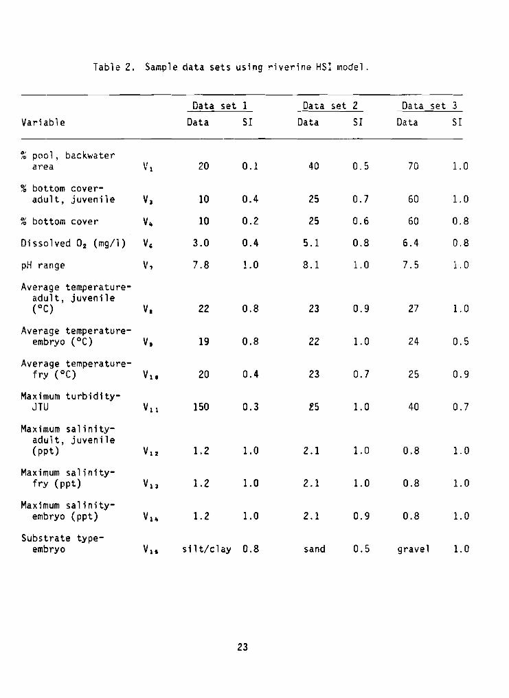
Table 2. Sample data sets using riverine H5I model.

Data set 1 Data set 2 Data set 3

Variable Data SI Data 51 Data 51

% pool, backwaterarea Vi 20 0.1 40 0.5 70 1.0

~, bottom cover-adult, juvenile VI 10 0.4 25 0.7 60 1.0

~~ bottom cover V,. 10 0.2 25 0.6 60 0.8

Dissolved O2 (mg/l) V, 3.0 0.4 5.1 0.8 6.4 0.8

pH range V, 7.8 1.0 8.1 1.0 7.5 1.0

Average temperature-adult, juvenile(OC) V. 22 0.8 23 0.9 27 1.0

Average temperature-embryo (OC) V, 19 0.8 22 1.0 24 0.5

Average temperature-fry (OC) Vu 20 0.4 23 0.7 25 0.9

Maximum turbidity-JTU Vll 150 0.3 f5 1.0 40 0.7

Maximum salinity-adult, juvenile(ppt) VlZ 1.2 1.0 2.1 1.0 0.8 1.0

Maximum salinity-fry (ppt) VlJ 1.2 1.0 2.1 1.0 0.8 1.0

Maximum salinity-embryo (ppt) Vu 1.2 1.0 2.1 0.9 0.8 1.0

Substrate type-embryo Vu sl1 tiel ay 0.8 sand 0.5 gravel 1.0

23

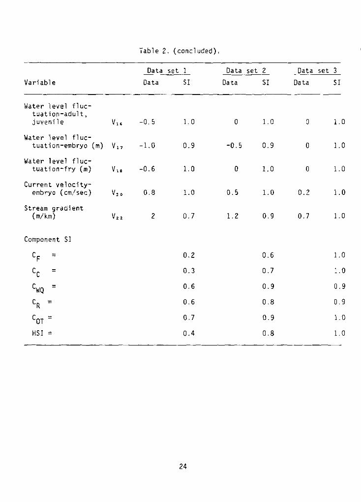
Table 2. (concluded).

Data set 1 Data set 2 Data set 3

Variable Data 51 Data S1 Data 51

Water 'Ievel fluc-tuat ion-adult,juvenil e V16 -0.5 1.0 a 1.0 0 1.0

Water level fluc-tuation-embryo (m) V17 -1.0 0.9 -0.5 0.9 0 1.0

Water level fluc-tuation-fry (m) Vl8 -0.6 1.0 0 1.0 a 1.0

Current velocity-embryo (em/sec) Vz o 0.8 1.0 0.5 1.0 0.2 1.0

Stream gradient(m/km) V2 2 2 0.7 1.2 0.9 0.7 1.0

Component S1

CF = 0.2 0.6 1.0

Cc = 0.3 0.7 1.0

CWQ = 0.6 0.9 0.9

CR = 0.6 0.8 0.9

COT = 0.7 0.9 1.0

HSI = 0.4 0.8 1.0

24

Table 3. Sample data sets using lacustrine HSI model.

Data set 1 Data set 2 Data set 3

Variable Data S1 Data S1 Data S1

~~ lacustrine area5. 6 m depth V2 5 0.2 15 0.6 65 0.9

0' bottom cover10

adult , juvenile V3 5 0.3 30 0.8 75 0.8

0' bottom cover10

( fry) V4 5 0.1 30 0.7 75 1.0

Average TDS (ppm) Vs 50 0.4 20 0.2 200 1.0

Dissolved O2 r 11 ) V6 (;.5 0.8 7.0 0.8 6.4 0.8\ mg:

pH range V7 8.2 1.0 8.7 0.5 7.9 1.0

Average temperature-adult, juvenile(OC) Va 21 0.7 28 1.0 26 1.0

Average temperature-embryo (OC) Vg 20 1.0 25 0.3 23 0.8

Average temperature-fry (0C) VlD 22 0.6 27 1.0 25 0.9

Maximum turbidity(ppm) VII 15 1.0 70 0.7 25 1.0

Maximum salinityadult, juvenile(ppt) V12 1.3 1.0 1.5 1.0 0.5 1.0

Maximum salinity(ppt) V13 1.3 1.0 1.5 1.0 0.5 1.0

25

Table 3. (concluded).

Data set 1 Data set 2 Data set 3

Variable Data SI Data SI Data SI

Maximum sa1i nity( ppt) VIS 1.3 1.0 1.5 1.0 0.5 1.0

Substrate type-embryo V15 sand 0.5 gravel 1.0 sil tiel ay 0.8

Water level fluc-tuati on-adult,embryo (01) V16 -5 0.7 0 1.0 0 1.0

Water level fluc-tuation-embryo (01) V17 +2 0.9 +0.3 1.0 0 1.0

Water level fluc-tuation-fry (01) V18 -5 0.3 0 1.0 0 1.0

Component SI

CF = 0.4 0.2 1.0

Cc = 0.3 0.8 0.9

CWQ = 0.8 0.8 0.9

CR = 0.5 0.7 0.9

HSl = 0.5 0.5 0.9

26

Model 2

Assuming water quality is adequate, optimal lacustrine habitat for large­mouth bass may be characterized as follows: fertile eros levels 100-350 ppm)lakes; abundant (40-80% of littoral area) bottom cover; warm (24-30° C) mid­summer water temperatures; and extensive (25-60% for northern latitudes; ~ 25%for southern latitudes) shallow (~ 6 m depth) areas.

HSI = Number of above criteria present- 4

Model 3

Use the regression models for largemouth bass standing crop in reservoirspresented by Aggus and Morais (1979) to calculate an HSI.

REFERENCES

Aggus, L. R., and G. J. Elliot. 1975. Effects of cover and food on year-classstrength of largemouth bass. Pages 317-322 in H. Clepper, ed. Blackbass biology and management. Sport Fish. Inst., Washington, D. C.

Aggus, L. R., and D. 1. Morais. 1979. Habitatfor reservoi rs ba sed on standi ng crop ofProg. Rep. to U.S. Fish Wildl. Serv.,Ft. Collins, Colorado. 120 pp.

suitability index equationsfish. Natl. Reservoir Res.Habitat Evaluation Proj.,

Allan, R. C., and J. Romero. 1975. Underwater observations of largemouthbass spawning and survival in Lake Mead. Pages 104-112 in H. Clepper,ed. Black bass biology and management. Sport Fish. Inst--:-: Washington,D.C.

Anderson, R. O. 1975. Factors influencing the quality of largemouth bassfishing. Pages 183-194 in H. Clepper, ed. Black bass Biology and Manage­ment. Sport Fish. Inst. ;Washington, D. C.

. 1981. Personal communication. Missouri Cooperative Fishery----:-:----:--=--=-

Unit, Columbia, Missouri.

Badenhuizen, T. R. 1969. Effect of incubation temperature on mortality ofembryos of the largemouth bass Micropterus salmoides (Lacepede). M.S.Thesis, Cornell Univ., Ithaca, New York. 88 pp.

Bailey, R. M., and C. L. Hubbs. 1949. The black basses (Micropterus) ofFlorida, with description of a new species. Univ. Michigan Mus. Zool.,Occas. Pap. 516. 43 pp.

27

Bailey, R. M., H. E. Winn, and C. L. Smith. 1954. Fishes from the EscambiaRiver, Alabama and Florida, with ecologic and taxonomic notes. Pr-cc ,Acad. Nat. Sci., Philadelphia 106:109-164.

Bennett, G. W. 1937. The growth of the largemouthed black bass, Hurosalmoides (Lacepede), in the waters of Wisconsin. Copeia 1937(2):104-118.

. 1971. Management of lakes and ponds. 2nd Ed. Van NostrandReinhold Co , , New York. 375 pp.

Bottroff, L. J. 1967. Integradation of Florida bass in San Diego County,California. M.S. Thesis, San Diego State Col1., San Diego, CA. 135 pp.

Branson, B. A. 1967. Fishes of the Neosho River system in Oklahoma. Am.Midl. Nat. 78:126-154.

Brungs, W. A., and B. R. Jones. 1977. Temperature criteria for freshwaterfish: protocol and procedures. U.S. Environ. Protection Agency, Environ.Res. Lab. Eco1. Res. Ser. EPA-600/3-77-061. 139 pp.

Buck, D. H. 1956a. Effects of turbidity on fish and fishing. Oklahoma Fish.Res. Lab. Rep. 56. 62 pp.

1956b. Effects of turb td ity on fish and fishing. Trans. N.Am. Wildl. Conf. 21:249-261.

Buck, D. H., and C. F. Thoits, III. 1970. Dynamics of one-species populationsof fishes in ponds subjected to cropping and additional stocking.Illinois Nat. Hist. Surv. Bull. 30:68-165.

Bulkley, R. V. 1975. Chemical and physical effects on the centrarchid basses.Pages 286-294 in H. C1 epper, ed. B1 ad bass bi 01 ogy and management.Sport Fish. Ins~, Washington, D. C.

Calabrese, A. 1969. Effect of acids and alkalies on survival of b1uegillsand largemouth bass. U.S. Bur. Sport Fish. Wi1d1. Tech. Paper 42.10 pp.

Car1ander, K. D. 1977. Largemouth bass. Pages 200-275 in Handbook of fresh­water fishery biology. Iowa State Univ. Press, Ames. Vol. 2.

Carlson, A. R., and J. G. Hale. 1972. Successful spawning of largemouth bassMicropterus sa1moides (Lacepede) under laboratory conditions. Trans. Am.Fish. Soc. 101:539-542.

Carr, M. H. 1942. The breeding habits, embryology and larval development ofthe 1argemouthed black bass in Florida. Proc. New England Zool. Club20:43-77.

28

Clugston, J. P. 1964. Growth of the Florida largemouth bass.salmoides floridanus (Lesueur), and the northern largemouthsalmoides (Lacepede), in subtropical Florida. Trans. Am.93:146-154.

Micropterusbass, M. s.Fish. -Soc.

1966. Centrarchid spawning in the Florida everglades. Q. J.Florida Acad. Sci. 29:137-144.

Coutant. C. C. 1975. Responses of bass to natural and artificial temperatureregimes. Pages 272-285 ~ H. Clepper, ed. Black bass biology and manage­ment. Sport Fish. Inst., Washington, D.C.

Cowardin, L. M., V. Carter, F. C. Golet, and E. T. LaRoe. 1979. Classifica­tion of wetlands and deepwater habitats of the United States. USDI FishWildl. Serv., FWS/OBS-79/31. 103 p.

Dahlberg, M. L., D. L. Shumway, and P. Doudoroff. 1968. Influence of dis-solved oxygen and carbon dioxide on swimming performance of largemouthbass and coho salmon. J. Fish. Res. Board Can. 25:49-70.

Deacon, J. E. 1961. Fish populations, following a drought, in the Neosho andMarais des Cygnes Rivers of Kansas. Univ. Kansas Mus. Nat. Hist. Publ.13:359-427.

Dudley, R. G. 1969. Survival of largemouth bass embryos at low dissolvedoxygen concentrations. M.S. Thesis, Cornell Univ., Ithaca, New York.61 pp.

Eipper, A. W., and H. A.. Regier. 1962. Fish management in New York farmponds. Cornell Ext. Bull. 1089. 40 pp.

Emig, J. W. 1966. Largemouth bass. Pages 332-353 in A. Calhoun, ed. Inlandfisheries management. California Fish Game. -

Finnell, J. C., R. M. Jenkins, and G. E. Hall. 1956. The fishery resourcesof the Little River system, McCurtain County, Oklahoma. Oklahoma Fish.Res. Lab. Rep. 55. 82 pp.

Funk, J. L.bass.ment.

1975. Structure of fish communities in streams which containPages 140-153 in H. Clepper, ed. Black bass biology and manage­

Sport Fish. Inst:, Washington. D.C.

Hardin, T., and K. Bovee. 1978. Largemouth bass. Instream Flow Group, U.S.Fish Wildl. Serv., Western Energy and Land Use Team, Ft. Collins,Colorado. Unpublished data.

Harlan, J. R., and E. B. Speaker. 1956. Iowa fish and fishing. 3rd Ed.State of Iowa. 377 pp.

Hart, J. S. 1952. Geographic variations of some physiological and morphol-ogical characters in certain freshwater fish. Univ. of Toronto Bio1.Ser. 60, Pub1. Onto Fish. Res. Lab. 72. 79 pp.

29

Heman. M. L., R. S. Campbell, and L. C. Redmond. 1969. ~1anipulation of fishpopulations through reservoir drawdown. Trans. Am. Fish. Soc. 98:293-304.

J~nkins, R. M. 1976. Prediction of fish production in Oklahoma reservoirs onthe basis of environmental variables. Ann. Oklahoma Sc. 5:11-20.

Jenkins, R. M., E. M. Leonard, and G. E. Hall. 1952. An investigation of thefi sheri es resources of the III i noi s Ri ver and pre-impoundment study ofTenkiller Reservoir. OKlahoma. Oklahoma Fish. Res. Lab. Rep. 26. 136 pp.

Jester, D. B., T. M. Moody, C. Sanchez, Jr., and D. E. Jennings. 1969. Astudy of game fish reproduction and rough fish problems in Elephant ButteLake. New Mexico Job Compl. Rep. Fed. Aid. Proj. F-22R-9, Job F-l.73 pp. (Cited by Carlander 1977).

Johnson, M. G., and W. H. Charlton. 1960. Some effects of temperature on themetabolism and activity of largemouth bass, Micropterus salmoidesLacepede. Prog. Fish. Cult. 22:155-163.

Kallemeyn, L. W., and J. F. Novotny. 1977. Fish and fish food organisms invarious habitats of the Missouri River in South Dakota, Nebraska, andIowa. USDI Fish Wildl. Serv., FWS/OBS-77/25.

Katz, M., A. Pritcherd, and C. E. Warren. 1959. Ability of some salmoidesand a centrarchid to swim in water of reduced oxygen content. Trans. Am.Fish. Soc. 88:88-95.

Kelley, J. W. 1968.mouth bass eggs.

Effects of in~ubation temperature on survival of large­Prog. Fish-Cult. 30:159-163.

Kilby, J. D. 1955. The fishes of two gulf coastal marsh areas of Florida.Tulane studies in Zoology 2:175-247.

Kramer, R. H., and L. L. Smith, Jr. 1960. First-year growth of the largemouthbass, Micropterus salmoides (Lacepede), and some related ecologicalfactors. Trans. Am. Fish. Soc. 89:222-233.

La Faunce, D. A., J. B. Kimsey, and H. K. Chadwick. 1964. The fishery atSutherland Reservoir, San Diego County, California. California Fish Game50: 271-291.

Larimore, R. W., and P. W. Smith. 1963. The fishes of Champaign County,Illinois, as affected by 60 years of stream changes. Illinois Nat. Hist.Surv. Bull. 28:299-382.

Laurence, G. C. 1972.larval largemouth4(1):73-78.

Comparative swimming abilities of fed and starvedbass (Micropterus salmoides). J. Fish. Biol.

MacCrimmon, H. R., and W. H. Robbins. 1975. Distribution of the black bassesin North America. Pages 56-66 in H. Clepper, ed. Black bass biology andmanagement. Sport Fish. Inst., Washington, D.C.

30

Macleod. J. C. 1967. ,!1, new apparatus for measuring maximum swimming speedsof small fish. J. Fish. Res. board Can. 24:1241-1252.

McCormick. ,J. H.• and J. A. Itiegner.different latitudes to elevatedSoc. 110:417-429.

1981.water

Responses of largemouth bass fromtemperatures. Trans. Am. Fish.

r·1iller. K. D., and R. H. Kramer. 1971. Sp awn i riq and early' life hi s t orv oft ar ccmouch bass U1-icropterus s a l mo i de s ) in l.a ke Pcwel1. Pages 73-33 inG. E. Hall. .Reservoir-fisheries--and- limnology. ,J\m. Fi sh . Soc. Spec.Publ. 8.

Miller, R. J. 1975. Comparative behavior of centrarchid basses.in H. Clepper, ed. Black bass biology and management.Tnst., Washington, D.C.

Pages 85-94Sport Fi sh.

Mohler, S. H. 1966.and smallmouth99 pp.

Comparative seasonal growth of the largemouth, spottedbass. M.S. Thesis, Univ. of Missouri, Columbia, Mo.

Morgan, G. D. 1958. A study of six different pond stocking ratios of large-mouth bass, Micr'Q£.1~rus salmoide~ (lacepede), and bluegill, lepomismacrochirus (Rafinesque); and the relation of the chemical, physical, andbiological data to pond balance and productivity. J. Sci. lab. DenisenUniv. 44:151-202.

Moss, D. D., and D. C. Scott. 1961. Dissolved oxygen requirements of threespecies of fish. Trans. Am. Fish. Soc. 90:377-393.

Moyle, P. B., and R. D. Nichols. 1973. Ecology of some native and introducedfi shes of the Si erra Nevada foothi 11 sin centra 1 Cal iforn i a. Cope i a1973:478-490.

Mraz, D. 1964. Observations on large and smallmouth bass nesting and earlylife history. Wisconsin Conserv. Dept., Res. Rep. 11 (Fisheries).13 pp.

Mraz, D., and E. l. Cooper. 1957. Reproduction of carp, largemouth bass,bluegills, and black crappies in small rearing ponds. J. Wildl. Manage.21:127-133.

Mraz, D., S. Kmiotek, and l. Frankenberger. 1961. The largemouth bass, itslife history, ecology and management. Wisconsin Conserv. Dept. Publ. 232.15 pp.

Muncy, R. J., G. J. Atchison, R. V. Bulkley. B. W. Menzel,C. Summerfe 1t. 1979. Effects of suspended so 1ids andduction and early life of warmwater fishes: a review.Protection Agencj EPA-600/3-79-042. 101 pp.

31

l. G. Perry, and R.sediment on repro­U.S. Environmental

Newell, A. E. 1960. Biological survey of the lakes and ponds in Coos, Graftonand Carroll Count i e s , New Hampshire Fish Game Surv. Rep. 8a. 297 pp.

Olmstead, L. L. 1974. The ecology of largemouth bass (Micropterus salmoides)and spotted bass (Micropterus punctulatus) in Lake Fort Smith, Arkansas.Ph.D. Dissertation, Univ. Arkansas, Fayetteville, Ak. 133 p.

Petit, G. D. 1973. Effects of dissolved oxygen on survival and behavior ofselected fishes of we s t e rn Lake Erie. Ohio 8iol. Surv. Bull. 4(4):1-76.

Ramsey, J. S. 1975. Taxonomic history and systematic relationships amongspecies of !:1lcfQQter~.? Pages 67-75 JJl H. Clepper, ed. Black bassbiology and management. Sport Fish. Inst., Washington, D.C.

Robbins, W. H., and H. R. MacCrimmon. 1974. The blackbass in America andoverseas. Publ. Div., Biomanagement and Research Enterprises, Ontario.196 pp.

Robinson, D. W. 1961. Utilization of spawning box by bass. Prog. Fish-Cult.23:119.

Saiki, M. K., and J. C. Tash. 1979. Use of cover and dispersal by crayfishto reduce predation by largemouth bass. Pages 44-48 In D. L. Johnson andR. A. Stein, eds. Response of fish to habitat structure in standingwat e r . N. Cent r a l T) i v. Am. Fish. Soc. Spec. Pub1. 6.

Scott, W. B., and E. J. Crossman. 1973. Freshwater fishes of Canada. Fish.Res. Board Can. Bull. 184. pp. 734-740.

Smitherman, R. O. 1975. Experimental species associations of basses inAlabama ponds. Pages 76-84 in H. Clepper, ed. Black bass biology andmanagement. Sport Fish. Inst.~,~Washington, D.C.

Snow, H. E. 1971. Harvest and feeding habits of largemouth bass in MurphyFlowage, Wisconsin. Wise. Dept. Nat. Resour. Tech. Bull. 50. 25 p.

Stewart, N. E., D. L. Shumway, and P. Doudoroff. 1967. Influence of oxygenconcentration on the growth of juvenile largemouth bass. J. Fish. Res.Board Can. 24:475-494.

Strawn, K. 1961. Growth of largemouth bass fry at various temperatures.Trans. Am. Fish. Soc. 90:334-335.

Stroud, R. H. 1967. Water quality criteria to protect aquatic life: asummary. Am. Fish. Soc. Spec. Publ. 4:33-37.

Summerfelt, R. C. 1975. Relationship between weather and year-class strengthof largemouth bass. Pages 166-174 in H. Clepper, ed. Black bass biologyand management. Sport Fish. Inst., Washington, D.C.

Swingle, H. S. 1956. Determination of balance in farm fish ponds. Trans. N.Am. Wildl. Conf. 21:298-322.

32

Swi ngl e, H0 So, and Eo V. Smith. 19500 Factors affecting the reproduct i or ofbluegill bream and largemouth black bass in ponds. Agr. Exp. Stn. AlabamaPolytechnic Inst. Circ. 87. 8 ppo

Tebo, L. B.• Jr., and E. G. McCoy. 1964. Effect of sea-water concentrationon the reproduction and survival of largemouth bass and bluegills. Prog.Fish-Cult. 26:99-106.

Trautman,Oh 0

M. B.683 pp.

19:'7. The fishes of Ohio. Ohio State Univ. Press, Columbus,

Venables, B. J., L. D. Fitzpatrick, and W. D. Pearson. 1978. Laboratorymeasurement of preferred body temperature of adult largemouth bass(Micropterus salmoides). Hydrobiologia 58(1):33-36.

Whitmore, C. M., C. E. Warren, and P. Doudoroff. 1960. Avoidance reactionsof salmonid and centrarchid fishes to low oxygen concentrations. Trans.Am. Fish. Soc. 89:17-26.

Winter, J. D. 1977.largemouth bass106:323-330.

Summer home range movementsin Mary Lake, Minnesota.

and habi tatTran s. Am.

use byFish.

fOIJr

Soc.

Zweiacker, P. L., and R. C. Summerfelt. 1974. Seasonal variation in food anddiet periodicity in feeding of northern largemouth bass, Micropterussalmoides salmoides (Lacepede), in an Oklahoma reservoir. Proc. South­eastern Assoc~r1i""eand Fish Comm. 27(1973):579-591.

33

5027'2 101.REPORT DOCUMENTATION . 1. REPORT NO. :2. 3. Recipient's Accession No •

PAGE i ~WS/OBS-82/l0.l6 iI

4. Tit'e and Subtitle 5. Report Date

IJuly 1982

Ha bi ta t Sui ta bil ity Index Models: Largemouth bass 16•

\8. Performing Organization Rept. No.7. Author(~l

Robert J. Stuber, Glen Gebhart and O. Eugene Maughani

9. Performing O"anization Name and Address Habitat Evaluation Procedures Group 110. Project/Task/WOrK Unit No.I

Western Energy and Land Use Team I

U.S. Fish and Wildlife Service r 11. Cont..ct(C) or Grant(G) No.

Drake Creekside Building One I(Cl

2625 Redwing Road i (GlI=nV't rnllinc: rnl .J Ant;?h I

12. Spon~oring Organization Name and Address Western Energy and Land Use Team i 13. Type of Report & Period Covered

Office of Biological ServicesFish and Wildlife Service I IU.S. Department of the Interi or i 14.

I

Washington, DC 20240 I15. Supplementary Notes

·1l5. Abstract (Limit: 200 words)

This is one of a series of publications that provi de information on the habi ta t I

requirements of selected fish and wildlife species. Literaure describing theIrelationship between habitat variables rel ated to life requisites and habitat

suitability for the Largemouth bass (Micropterus salmoides) are synthesized. These I

data are subsequently used to develop Habitat Suitability (HSI) models. The HSImodels are designed to provide information that can be used in impact assessmentand habitat management.

I

17. Document Analysis a. Descriptors ,

'Animal behavior ' Mathematical models-Animal ecology"Bass'Fishes-Hab i tab t l t ty

b. Identifiers/OQen-End&d Terms

Largemouth bass Habitat Suitability Index modelsMi cropterus salmoides Habitat requirementsHabitat suitability Species-habitat relationshipsHabitat preference Impact assessmentHabitat management

c. COSATI Field/Group

:8. AvaIlability Statement 19. Security Class (This Reoortl 2l. No. of Pages

UNCLASSIFIED i i I- v +RPiUnl imi ted20. SeCUrlty Class (This Pa!lel 22. Price

UNCLASSIFIED(Se. ANSI-Z39.13)

~u.s. GOVERNMENT PAINTING OFFICE:1982-5llO-617 I 417

See Instruetions on Reyerse OPTIONAL FOR'" 272 ,4-77)(Formerly NTIS-3S)Department of Comml!ree

•

••• ..__ ....J~.

' .'· 0 ,,-

Hawaiian Islands (>

-(:( Headq uarters . Division of BiologicalServices, Wasnington, DC

x Eastern Energy anO Land Use TeamLeetown , WV

* Nationa l Coastal Ecosystems TeamSli dell , LA

• Western Energy and Land Use TeamFt. Coll ins . CO

• Locat ions of Regional Off ices

REGION 1Regional DirectorU,S. Fish and Wildlife ServiceLloyd Five Hundred Building, Suite 1692500 N.E. Multnomah StreetPortland , Oregon 97232

REGION 4Regional DirectorU.S. Fish and Wildlife ServiceRichard B. Russell Building75 Spring Street , S.W.Atlanta, Georgia 30303

IJ- - - ----

6 1r-- - -~-

L, JI : - ~- --I I

1- - -'I Il,_I 2 ,,-~--

-_.J

REGION 2Regional DirectorU.S. Fish and Wildlife ServiceP.O. Box 1306Albuquerque, New Mexico 87 103

REGION 5Regional DirectorU.S. Fish and Wildlife ServiceOne Gateway Cente rNewton Corner, Massachusetts 02158

REGION 7Regional DirectorU.S. Fish and Wildlife ServicelOll E. Tudor RoadAnchorage, Alaska 99503

- ..~,.

REGION 3Regional DirectorU.S. Fish and WildlifeServiceFederal Building, Fort SnellingTwin Cities, Minnesota 551 J I

REGION 6Regional DirectorU.S. Fish and Wildli fe ServiceP.O. Box 25486Denver Federal CenterDenver, Colorado 8022 5

u.s.FISH ..WILDLIFE

f>ERVICE

DEPARTMENT OF THE INTERIOR hi?]u.s.FISH ANDWILDLIFESERVICE ~

"'-r rw T " "

As the Nat ion's pri ncipal conservation agency, the Department of the Interior has respon­sibility for most of our ,nationally owned public lands and natural resources . This includesfostering the wisest use of our land and water resources, protecting our fish and wildlife,preserving th & environmental and cultural values of our national parks and historical places,and providing for the enjoyment of life through outdoor recreation. The Department as­sesses our energy and mineral resources and works to assure that t heir development is inthe best interests of all our people. The Department also has a major respons ibility forAmerican Indian reservation communit ies and for people who live in island territories underU.S. adm inist ration.