LibraryNa t onal ~e tland esearch CenterU. S. Flsr, a cWlldHf ~ ervlce7 0 Caj 11 0 ie D ' leva dLafay tte, La. 70506

BIOLOGICAL REPORT 82(10.89)DECEMBER 1984

HABITAT SUITABILITY INDEX MODELSAND INSTREAM FLOW SUITABILITYINDEX CURVES: WHITE BASS

- h and Wildlife Service

;. Department of the InteriorsK361. U5 4no. 82 ­10 .89

This is one of the first reports to be published in the new "BiologicalReport" series. This technical report series, published by the Researchand Development branch of the U.S. Fish and Wildlife Service, replacesthe "FWS/OBS" series published from 1976 to September 1984. The Biolog­ical Report series is designed for the rapid publication of reports withan application orientation, and it continues the focus of the FWS/OBSseries on resource management issues and fish and wildlife needs.

MODEL EVALUATION FORM

Habitat models are designed for a wide variety of planning applica­tions where habitat information is an important consideration in thedecision process. However, it is impossible to develop a model thatperforms equally well in all situations. Assistance from users andresearchers is an important part of the model improvement process. Eachmodel is published individually to facilitate updating and reprinting asnew i nformat i on becomes avail ab 1e. User feedback on model performancewill assist in improving habitat models for future applications. Pleasecomplete this form following application or review of the model. Feelfree to inc 1ude addit i ona 1 i nformat i on that may be of use to ei ther amodel developer or model user. We also would appreciate 'information onmodel testing, modification, and application, as well as copies of modifiedmodels or test results. Please return this form to:

Habitat Evaluation Procedures Groupor

Instream Flow GroupU.S. Fish and Wildlife Service2627 Redwing Road, Creekside OneFort Collins, CO 80526-2899

Thank you for your assistance.

Species _

Habitat or Cover Type(s)

GeographicLocation

Management Action AnalysisType of Application: Impact AnalysisBaseline Other -------------------------

Variables Measured or Evaluated

Was the species information useful and accurate? Yes No

If not, what corrections or improvements are needed?----------

Were the variables and curves clearly defined and useful? Yes No

If not, how were or could they be improved?

Were the techniques suggested for collection of field data:Appropriate? Yes NoClearly defined? Yes NoEasily applied? Yes No

If not, what other data collection techniques are needed?

Were the model equations logical? Yes NoAppropriate? Yes No

How were or could they be improved?

Other suggestions for modification or improvement (attach curves,equations, graphs, or other appropriate information)

Additional references or information that should be included in the model:

Model Evaluater or Reviewer

Agency

Address

Date-------------

Telephone Number Comm:------------ FTS

Biological Report 82(10.89)December 1984

HABITAT SUITABILITY INDEX MODELS AND INSTREAM FLOWSUITABILITY INDEX CURVES: WHITE BASS

by

Karen HamiltonHabitat Evaluation Procedures GroupWestern Energy and Land Use Team

U.S. Fish and Wildlife ServiceDrake Creekside Building One

2627 Redwing RoadFort Collins, CO 80526-2899

and

Patrick C. NelsonInstream Flow and Aquatic Systems Group

Western Energy and Land Use TeamU.S. Fish and Wildlife Service

Drake Creekside Building One2627 Redwing Road

Fort Collins, CO 80526-2899

Western Energy and Land Use TeamDivision of Biological Services

Research and DevelopmentFish and Wildlife Service

U.S. Department of the InteriorWashington, DC 20240

This report should be cited as:

Hamilton, K., and P. C. Nelson. 1984. Habitat suitability index models andinstream flow suitability index curves: White bass. U.S. Fish Wildl.Servo 8iol. Rep. 82(10.89). 35 pp.

PREFACE

Information presented in this document is for use with the HabitatEvaluation Procedures (HEP) and the Instream Flow Incremental Methodology(IFIM). The information also should be useful for impact assessment and fordeveloping management recommendations and mitigation alternatives for thespecies using methodologies other than HEP or IFIM. The comparison andrecommendations for use of HEP and I FIM presented by Armour et a1. (1984) 1should help potential users of these two methodologies determine the mostefficient way to utilize the information in this publication.

The Suitability Index (SI) curves and graphs and Habitat Suitability Index(HSI) models presented in this report are based primarily on a synthesis of-j nformat ion obta i ned from a revi ew of the 1i terature concerni ng the habi tatrequirements of the species. The HSI models and SI curves are scaled toproduce an index between 0 (unsuitable habitat) and 1 (optimal habitat).Assumptions used to transform habitat use information into an index are noted,and guidelines for application of the curves and models are described. Adiscussion of IFIM and white bass SI curves available for use with IFIM isincluded.

The SI curves and HSI models are starting points for users of HEP or IFIMto develop their own curves and models. Use of the SI curves and HSI modelswithin project-specific applicational constraints is likely to require modifi­cation of the SI curves or graphs and HSI models to meet those constraints andto be appl icable to local habitat conditions. Users of the SI graphs and/orHSI models with HEP should be familiar with the standards for developing HSImodels (U.S. Fish and Wildlife Service 1981)1 and the guidelines for simplify­ing HSI model s and recommended measurement techniques for model variables(Terrell et al. 1982; Hamilton and Bergersen 1984).1 Users of the SI curveswith IFIM should be familiar with the Guide to Stream Habitat Analysis (Bovee1982)1 and the User's Guide to the Physical Habitat Simulation System (Milhouset al. 1984).1 Material for use with IFIM is presented in English units ofmeasure because flow-related data are normally collected in English units.

The HSI models and SI curves are hypotheses of species-habitat relation­ships, not statements of proven cause and effect relationships. The curvesand models are based on the literature and professional judgment. They havenot been applied in the field. For this reason, the U.S. Fish and Wildlife

1Citation included in References.

i ; i

Service encourages model users to convey comments and suggestions that mayhelp us increase the utility and effectiveness of this habitat-based approachto fisheries planning. Please send comments to:

Habitat Evaluation Procedures Groupor

Instream Flow and Aquatic Systems GroupWestern Energy and Land Use TeamU.S. Fish and Wildlife Service2627 Redwing RoadFort Collins, CO 80526-2899

iv

CONTENTS

Page

PREFACE iiiACKNOWLEDGMENTS vi

HABITAT USE INFORMATION 1Genera 1 1Age, Growth, and Food 1Reproduction...................................................... 2Speci fi c Habitat Requi rements 2

HABITAT SUITABILITY INDEX (HSI) MODELS 5Model Applicability............................................... 5Mode 1 Descri pt ion - Lacustri ne 6Model Description - Riverine 7Suitability Index (SI) Graphs for Model Variables 9Lacustrine Habitat Suitability Index Equations.... 13Riverine Habitat Suitability Index Equations...... 14Interpret i ng Mode 1 Outputs 15

ADDITIONAL HABITAT MODELS 21Model 1 21Mode 1 2 21

INSTREAM FLOW INCREMENTAL METHODOLOGY (IFIM) 21Suitability Index Graphs as Used in IFIM 22Availability of Graphs for Use in IFIM 24

REFERENCES 31

ACKNOWLEDGMENTS

K. E. Erickson, Oklahoma Department of Wildlife Conservation, OklahomaCity; R. W. Luebke, Texas Parks and Wildlife Department, Ingram; and F. Vasey,Missouri Department of Conservation, Columbia, reviewed drafts of this documentand offered constructive suggestions. However, the reader should not construethese revi ews as an endorsement of the model contents. C. Short provi dededitorial assistance. Word processing was by C. J. Gulzow and D. E. Ibarra.The cover illustration was done by D. Raver, U.S. Fish and Wildlife Service.

vi

WHITE BASS (Morone chrysops)

HABITAT USE INFORMATION

General

The range of the white bass (Morone chrysops) originally was restrictedto the large lakes and rivers of the Great Lakes and Mississippi River drain­ages, with its center in the Lake Erie drainage (Van Oosten 1942; Sigler1949b). Depletion of white bass in the Great Lakes and increased stocking innewly constructed reservoi rs resul ted ina southward shi ft in its center ofabundance (Riggs 1955). This species is an excellent game fish in largereservoirs, and its range now reaches from coast to coast because of introduc­tions. It is a productive, easily harvested sport fish, particularly suitablefor reservoirs where fishing success for other species has declined (Jenkinsand Elkin 1957).

Age, Growth, and Food

Female white bass grow faster and get larger than males. Both sexes growfaster in southern regions than northern regions, but the average life span insouthern areas is only about 4 years (Howell 1945; Ward 1949; Thompson 1951;Tompkins and Peters 1951), compared to 7 to 10 years in northern regions(Forney and Taylor 1963; Priegel 1971). The fastest rate of growth occurs inthe first year, but white bass have demonstrated growth compensation the yearfollowing a season of reduced growth (Ruelle 1971). First-year growth rangesfrom 4 inches in the North to 8 inches (10 to 20 cm) in the South (Jenkins andElkin 1957). White bass weight increased an average of 0.60 lb (272 g)/year,with a range of 0.25 to 0.85 lb (113 to 385 g)/year, in Oklahoma reservoirsand lakes (Jenkins and Elkin 1957). Male white bass usually mature 1 yearearlier than females. In northern waters (approximately 40° north latitude),females mature at age II to IV (Sigler 1949a,b; Priegel 1971). In the South,they mature at age I to III (Tompkins and Peters 1951; Webb and Moss 1968).

White bass are opportunistic feeders. They form large schools near thewater's surface, moving in search of prey. Feeding activities of these schoolsare the most conspicuous when forage fish and emerging insects are concentrated(Pflieger 1975). The dominance of fish, benthic invertebrates, and zooplanktonin the di et of young-of-the-year can vary hourly, seasonally, and annually,depending on prey availability (Olmsted and Kilambi 1971; Ruelle 1971;Voigtlander and Wissing 1974). Larvae feed on zooplankton, selecting largerspecies as they grow (Ruelle 1971; Nelson 1980). Young white bass near 20 mmlong commonly eat macroinvertebrates, but piscivory has been observed in white

1

bass as small as 23 mm in length (Bonn 1953). Fish normally start to increasein di etary importance when the whi te bass reach about 40 mm long, oftenbecoming the dominant food item before the end of the first season of growth(Sigler 1949a,b; Ruelle 1971). White bass grow best when young percids,centrarchids, or clupeids are plentiful, and a piscivorous diet is initiatedsoon after hatching (Bonn 1953; Jenkins and Elkin 1957; Ruelle 1971).

Although adult white bass are usually piscivorous, they will readilychange to macroinvertebrates or even zooplankton when forage fish populationsare depleted (Sigler 1949a; Forney and Taylor 1963; Olmsted and Kilambi 1971;Voigtlander and Wissing 1974). Shad and alewife are preferred forage, andwhite bass production is high where large populations of these species exist(Jenkins and Elkin 1957; Moser 1968; Olmsted and Kilambi 1971; Ruelle 1971).

Reproduction

White bass spawn earl ier in the year than most fish species and preferrunning water for spawning (Bonn 1953; Jenkins and Elkin 1957; Chadwick et al.1966). However, they spawn over rocky shoals in lakes and reservoirs whentributary streams are not accessible (Bonn 1953). White bass have spawnedsuccessfully in Elephant Butte Reservoir (New Mexico), when the Rio GrandeRiver flows were inadequate (Jester 1971). In Lake McConaughy, Nebraska, theyspawn both in the reservoir and in the North Platte River (McCarraher et al.1971) .

When water temperatures reach 12 to 16° C, mature white bass form large,unisex schools and migrate to the spawning grounds', with the males arrivingseveral weeks before the females (Riggs 1955). White bass may home to aspecific site in the lake or reservoir (Hasler et al. 1969) or migrate as muchas 150 miles upstream from the reservoir (ChadWick et al. 1966).

Spawning begins when the water temperature reaches 12 to 24° C (Riggs1955; Webb and Moss 1968; Ruelle 1971). Webb and Moss (1968) observed thatspawning stopped when the temperature fell below 12° C and resumed when itrose above 12° C. Spawning lasts 5 to 25 days (Riggs 1955; Ruelle 1971). Theeggs are fertilized as they sink and then stick to gravel, rocks, or vegetation(Riggs 1955). White bass apparently prefer to spawn over a firm substrate inwater 0.5 to 6 m deep, most commonly at depths of 0.6 to 2 m (Riggs 1955;Chadwick et al. 1966; Webb and Moss 1968). White bass return to deeper waterimmediately after spawning.

White bass eggs develop quickly; Horrall (1961) reported that eggs hatchedin 45 h at 20.2° C and in 41 h at 21.5° C under laboratory conditions. Larvaein reservoi rs have been captured most often near the mouth of an inundatedstream used by spawning adults (Beckman and Elrod 1971; Storck et al. 1978).Thus, it is assumed that white bass larvae, after hatching, drift downstreamto a reservoir or lake or until they come to a riverine backwater.

Specific Habitat Requirements

Although white bass are native to large rivers, research has focused ontheir natural history in lentic waters, particularly reservoirs. Successful

2

populations have been found in waters that were turbid or clear (Thompson1951), deep or shallow, fluctuating or stable, and which ranged in size from162 to 37,337 hectares (Tompkins and Peters 1951; Jenkins and Elkin 1957;McNaught and Hasler 1961; Webb and Moss 1968; Olmsted and Kilambi 1971; Priegel1971; Ruelle 1971). However, white bass generally are associated with theepipelagic zone of moderately large to large lakes; important fisheries alsooccur in the tailwaters of some reservoirs (Chadwick et al. 1966; Walburget al. 1971) and in some streams during spawning migrations (Webb and Moss1968; Becker 1983).

Mount (1961) reported that a dissolved oxygen (DO) concentration of 1 ppmat 21 to 24° C was lethal to white bass. A concentration of 2 ppm wasextremely stressful and probably would have been lethal within 72 hrs. Therewas a pronounced decrease in activity and coloration and increased ventilationbelow 3 ppm. Because activity and the presence of toxic materials can raisethe DO concentration at which stress occurs, it is assumed that 5 ppm DO isthe lower optimum limit, as recommended for aquatic life by the U.S. Environ­menta 1 Protection Agency (1976) . Although some 1ent i c waters exhi bi thypolimnetic oxygen deficiencies, white bass inhabit the epilimnion where lowDO concentrations are uncommon or localized.

Upper and lower pH levels tolerated by white bass have not been investi­gated. The optimum pH range is assumed to be 6.5 to 9.0, based on recommenda­tions by the U.S. Environmental Protection Agency (1976).

White bass do not appear to be physiologically sensitive to normal levelsof total dissolved solids (TOS) or alkalinity, but the species may indirectlybenefit from dissolved solids ranging from approximately 100 to 800 mg/l.These levels often are associated with productive waters, and successfulpopulations of white bass are reported most often from waters within this TOSrange (e.g., Sigler 1949a,b; Tompkins and Peters 1951; Jenkins and Elkin 1957;Jester 1971; McCarraher et al. 1971; Walburg 1977). White bass toleratebrackish water but always spavin in fresh water. They have been reported todie when chlorides reached 6,000 ppm (Chadwick et al. 1966).

Turbidity has no observable effect on white bass spawning success, larvalsurvival, or growth (Jenkins and Elkin 1957; Jester 1971; Summerfelt 1971;Walburg 1976; Nelson 1980). However, they avoid areas with continuous turbid­ity and have become abundant in sections of rivers where impoundments havedecreased turbidity (Pflieger 1975).

A large forage fish population appears to be the key to a successfulwhite bass population (Jenkins and Elkin 1957; Chadwick et al. 1966). Shad(porosoma spp.) probably are the preferred forage, particularly threadfin shad(Q. petenense) because of its abundance, availability, and smaller size(Olmsted and Kilambi 1971). Gizzard shad e.Q. cepedianum) tolerate coldertemperatures and are more wi despread, but ei ther gi zzard or threadi n shadnearly always are present where white bass are abundant. Abundance of whitebass fluctuates in Ozark reservoirs in response to changes in the gizzard shadpopulation (Houser and Bryant 1970; Pflieger 1975). Yellow perch (Percaflavescens), alewife (Alosa pseudoharengus), emerald shiner (NotropTS

3

atherinoides), and bluegill (Lepomis macrochirus) also serve as forage species(Sigler 1949a,b; Walburg et al. 1971; Olmsted and Kilambi 1971; Kohler and Ney1981). The negative correlation between white bass harvest and water levelfluctuations in many reservoirs (Jenkins and Morais 1971) may be at leastpartially due to the negative effect of water level fluctuation on the repro­ductive success of forage fish (Nelson 1974; Walburg 1976).

Adult. Reproducing populations of white bass have been reported fromlakes as small as 81 hectares in Texas (Luebke, pers. comm.). Growth inOklahoma lakes smaller than 162 hectares was slower than growth in largerwaters (Jenkins and Elkin 1957). Growth was positively correlated with percentchange in surface area of Lake Oahe, South Dakota, but may have been indicativeof increased forage fish production with the increased littoral area (Nelson1974).

Summer temperatures in white bass habitats typically are 19 to 28° C(Gasaway 1970; Jester 1971; Nelson 1974; Kohler and Ney 1981). Growth isgreater in the South where these temperatures are rna i nta i ned for a longerperiod (Webb and Moss 1968). Thermal zones in the Wabash River created bycooling effluent from power plants were analyzed by Gammon (1973) for selectionand avoidance by white bass. He suggested that the probable opti-mum tem­perature for white bass lies between 28.0 and 29.5° C.

Data about white bass riverine habitat requirements are scarce in the1iterature. Kall emeyn and Novotny (1977) captured white bass in chutes,pools, and sand bars in unchannelized segments of the Missouri River and nearstructures, such as notched di kes and revetments, in channel i zed segments.Catch per unit effort was highest where water velocity was 0.6 to 0.7 m/sec,intermediate in areas with a velocity of 0.2 m/sec, and lowest in areas wherethe velocity was 0.4 to 0.5 m/sec or 0.9 to 1.0 m/sec. Depth at all sites was1 to 2 m.

White bass seem to be more sensitive to prey location than to habitatfeatures. For example, Gammon (1973) reported that white bass and gizzardshad both were concentrated in slow moving water. Similarly, emerald shinersoften were re 1at i vely abundant where white bass were caught in the Mi ssouriRiver (Kallemeyn and Novotny 1977), and gizzard shad accounted for the greatestpercentage of biomass where white bass were captured in the Mississippi River(Pennington et al. 1983).

Spawning/embryo. White bass prefer to spawn in running water but willspawn in lakes and reservoirs (Howell 1945; Bonn 1953; Riggs 1955; Jester1971; Walburg 1976). White bass will spawn over silt and mud, but rock,gravel, firm sand substrate, or vegetation is preferred (Sigler 1949b; Riggs1955; Webb and Moss 1968). Silt and mud are assumed to be less than optimumspawning substrates.

Water temperature must reach 12 to 14° C in the spring before spawningbegins (Riggs 1955; Webb and Moss 1968; Ruelle 1971). Embryo development andhatching was 2 to 4 days at 16 to 21° C under laboratory conditions (Horrall1961; Ruelle 1971; Siefert et al. 1974). Yellayi and Kilambi (1970) suggested

4

that 15.5 to 16.7° C was the optimum development temperature range, based onlaboratory culture of eggs. Embryo survival decreases when DO drops to 20%saturation or less (Siefert et al. 1974).

A large, rapid drop in water level can result in the exposure and loss of1arge numbers of eggs (Webb and Moss 1968) and reduced spawning success(Walburg 1976).

Larvae. White bass larvae are 2 to 3 mm in length at hatching (Ruelle1971). They drift with wi nd induced currents ina 1ake or downstream to anursery area where other small fish and invertebrates also are concentrated(Horrall 1961; Storck et al. 1978; Nelson 1980). The nursery area is usuallyan embayment of an impounded river, a sheltered bay, or a backwater.

Newly hatched larvae were captured most often at depths of 1 to 2 moversandy beaches; they avoided dense vegetation and organic bottoms (Moser 1968;Taber 1969; Wa'lburg 1976). Larvae greater than 10 mm in length were foundoffshore, near water that was 2 to 4 m deep, during the day (Taber 1969;Storck et al. 1978), but moved into shore at sunset to feed on zooplankton andinvertebrates until sunrise (Bonn 1953; Olmsted and Kilambi 1971; Voigtlanderand Wissing 1974).

Juvenile. Young-of-the-year growth is strongly correlated with tempera­ture and insect and forage fish availability (Jenkins and Elkin 1957; Ruelle1971; Walberg 1976; Kohler and Ney 1981). In lacustrine environments, juvenilewhite bass have the same habitat requirements as adults. However, juvenilesin riverine habitats seemed to be associated with slower water than adultsuntil they reached about 100 mm in length (Kallemeyn and Novotny 1977). Moser(1968) reported that juvenile white bass in lacustrine habitats were associatedwith sandy littoral areas.

HABITAT SUITABILITY INDEX (HSI) MODELS

Model Applicability

Geographic area. This model is applicable throughout the native andintroduced range of white bass in the 48 contiguous United States. Thestandard of comparison for each variable is the optimum value of the variablethat occurs anywhere within this region. The model will not provide an HSI of1.0 when applied to northern waters because day-degrees above 16° C (V s ) does

not reach the optimum values that occur in the southern portion of the range.

Season. The model provides a rating for a body of water based on itsability to support a reproducing population of white bass throughout the year.

Cover types. The model is applicable to riverine and lacustrine habitats,as described by Cowardin et al. (1979).

5

Verification level. The model has not been tested in the field. Themodel produces an index between 0 and 1 that we believe should have a positiverelationship with spawning success, growth, and standing crop of adults,juveniles, and larvae.

Model Description - Lacustrine

The success of a white bass populat i on appears to be most stronglyaffected by the quantity and quality of the food source and by the availabilityof spawning sites. The model is used to evaluate the ability of the habitatto meet food and reproduction requirements. Habitat variables that have beenassociated with growth, standing crop, and feeding behavior are included inthe model. The relationships between the habitat variables and life requisitecomponents of the model for lacustrine conditions are diagrammed in Figure 1.

Habitat variables Life requisites

Forage fish (Va) ------------Food----,

Water level change (V4 ) --- - ,

Temperature (V 6 ) --------+---Reproduction -+----------- HSI

Length and depth ratio (V 9 )

Percent spawning habitat (V1 0 )

Surface area (V 1 ) - - - - - --,

Day-degrees (Vs ) ------+----- Other

Substrate index (V,)-----

Figure 1. Tree diagram illustrating relationships between modelvariables, model components, and an HSI for white bass inlacustrine environments.

6

It is assumed that the water quality standards defined by the U.S.Envi ronmenta1 Protection Agency (1976) for aquatic 1ife apply to whi te bass.Specifically, the optimum range for dissolved oxygen is ~ 5 mg/l, and theoptimum pH range is 6.5 to 9.0.

Food component. The speci es compos it i on and abundance of small foragefishes (Va) is important because they nearly always are the main food source

of a large, rapidly growing white bass population. Shad (Dorosoma spp.),particularly threadfin shad, are particularly desirable forage species.

Reproduction component. Water temperature determines the onset of spawn­ing and must be maintained for continued spawning and normal embryonic devel­opment (V 6 ) . There is some evidence that high temperatures permit fungal

growth, which kills the eggs (Yellayi and Kelambi 1970).

The percent habitat suitable for spawning (V l O ) is defined based on the

preference of whi te bass for the speci fi ed spawni ng substrates. It also isassumed that soft substrates could result in suffocation of the eggs. Whitebass prefer running water for spawning; therefore, this variable never receivesa Suitability Index (SI) of 1 because a lake or reservoir without a suitableriver spawning site is considered suboptimum. Accessible river spawninghabitat is described by V9 •

A change in water level (V 4 ) could expose the eggs and reduce the repro­

ductive success of both white bass and forage fish. The SI curve should beadjusted to reflect the potential effects of a water level change at a specificspawning site.

Other component. The "other" component contains variables that helpdescribe habitat suitability for reasons not easily classified into a singlecomponent described above. Surface area (V l ) is included because white bass

do not appear to survive or grow well in ponds or small impoundments. Day­degrees above 16° C (V s ) combines length of growing season and water tempera-

ture, both of which affect white bass growth. A substrate index, combinedwith depth curves, (V 7 ) is included because juvenile white bass prefer to

forage over sandy littoral or shoal areas, while deeper water is needed foroverwintering.

Model Description - Riverine

The riverine model includes the same components as the lacustrine model.However, stream order (V 2 ) is substituted for surface area to describe the

preference of white bass for large bodies of water. Percent area with acurrent velocity less than 0.4 m/sec (V]) is included because white bass are

rarely found in the mainstream and because forage fish occur in low velocityareas. The relationship between the habitat variables and life requisitecomponents of the model for riverine conditions are diagrammed in Figure 2.

7

Habitat variables Life requisites

Forage fi sh (Va) ----------- Food----,

Water level change

Temperature (V 6 )

Length:depth ratio

(V4

) ]1- _] Reproduction-+----------- HSI

(V g )

Stream order (V 2 ) ---~

% low velocity area (V 3 ) -

1--------- OtherDay-degrees (V s ) -------i

Substrate index (V7)---~

Figure 2. Tree diagram illustrating relationships between modelvariables, model components, and an HSI for white bass in riverineenvironments.

8

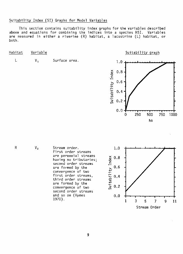
Suitability Index (SI) Graphs for Model Variables

This section contains suitability index graphs for the variables describedabove and equations for combining the indices into a species HSI. Variablesare measured in either a riverine (R) habitat, a lacustrine (L) habitat, orboth.

Habitat

l

Variable

Surface area.

Suitability graph

1.0

>< 0.8CLI"0£::......>, 0.6

+oJ.....r-..... 0.4..c

"'+oJ.....~ 0.2V)

0.0a 250 500 750 1000

ha

R Stream order.First order streamsare perennial streamshaving no tributaries;second order streamsare formed by theconvergence of twofirst order streams,third order streamsare formed by theconvergence of twosecond order streamsand so on (Hynes1970).

1.0

>< 0.8CLI"0£::......>. 0.6

+oJ.....r-

0.4......D

"'+oJ.....0.2~

V)

0.01 3 5 7 9 11

9

Stream Order

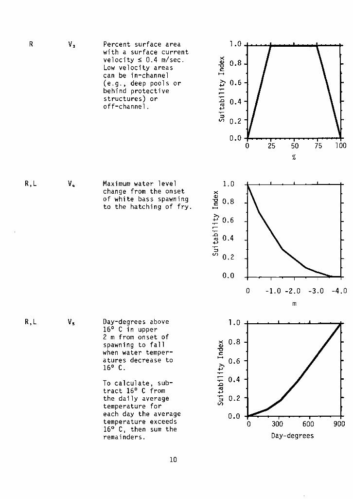
R Percent surface areawith a surface currentvelocity ~ 0.4 m/sec.Low velocity areascan be in-channel(e.g., deep pools orbehind protectivestructures) oroff-channe 1.

1.0

xQ) 0.8"'Ce......~ 0.6~.....r-.......0 0.4f1:l~......:::lVl 0.2

0.00 25 50 75 100

%

R,L V4 Maximum water level 1.0change from the onset xof white bass spawning Q)

"'C 0.8to the hatching of fry. e......

t' 0.6......r-........0 0.4f1:l~......:::l

V) 0.2

0.0

0 -1.0 -2.0 -3.0 -4.0

m

R,L Vs Day-degrees above 1.016° C in upper2 m from onset of

0.8spawning to fall xQ)

when water temper- "'Ce

atures decrease to ......0.6

16° C. ~~.....r- 0.4To calculate, sub- .......0

tract 16° C from f1:l~

the daily average ..... 0.2:::l

temperature for Vl

each day the average 0.0temperature exceeds 0 300 600 90016° C, then sum theremainders. Day-degrees

10

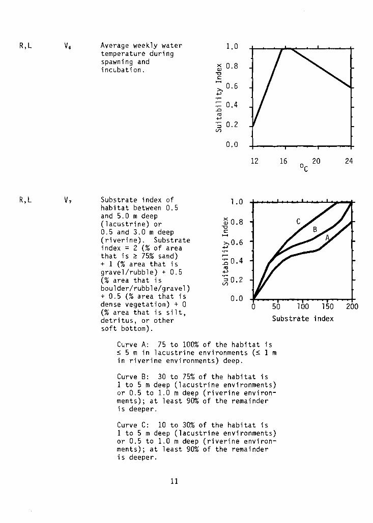
R,L Average weekly watertemperature duringspawning andincubation.

1.0

~ 0.8"'0s::......>, 0.6+-l'r-

0.4..0ttl

+-l

:::J 0.2V')

0.0

12 16 o 20C

24

200100 150

Substrate index

1.0

~ 0.8"'0s::......>, 0.6~'r-r-

:0 0.4ttl~

.; 0.2V')

0.00 50

Substrate index ofhabitat between 0.5and 5.0 m deep(lacustrine) or0.5 and 3.0 m deep(riverine). Substrateindex = 2 (% of areathat is ~ 75% sand)+ 1 (% area that isgravel/rubble) + 0.5(% area that isboulder/rubble/gravel)+ 0.5 (% area that isdense vegetation) + 0(% area that is silt,detritus, or othersoft bottom).

R,L

Curve A: 75 to 100% of the habitat is~ 5 m in lacustrine environments (~ 1 min riverine environments) deep.

Curve B: 30 to 75% of the habitat is1 to 5 m deep (lacustrine environments)or 0.5 to 1.0 m deep (riverine environ­ments); at least 90% of the remainderis deeper.

Curve C: 10 to 30% of the habitat is1 to 5 m deep (lacustrine environments)or 0.5 to 1.0 m deep (riverine environ­ments); at least 90% of the remainderis deeper.

11

I

l-

. -

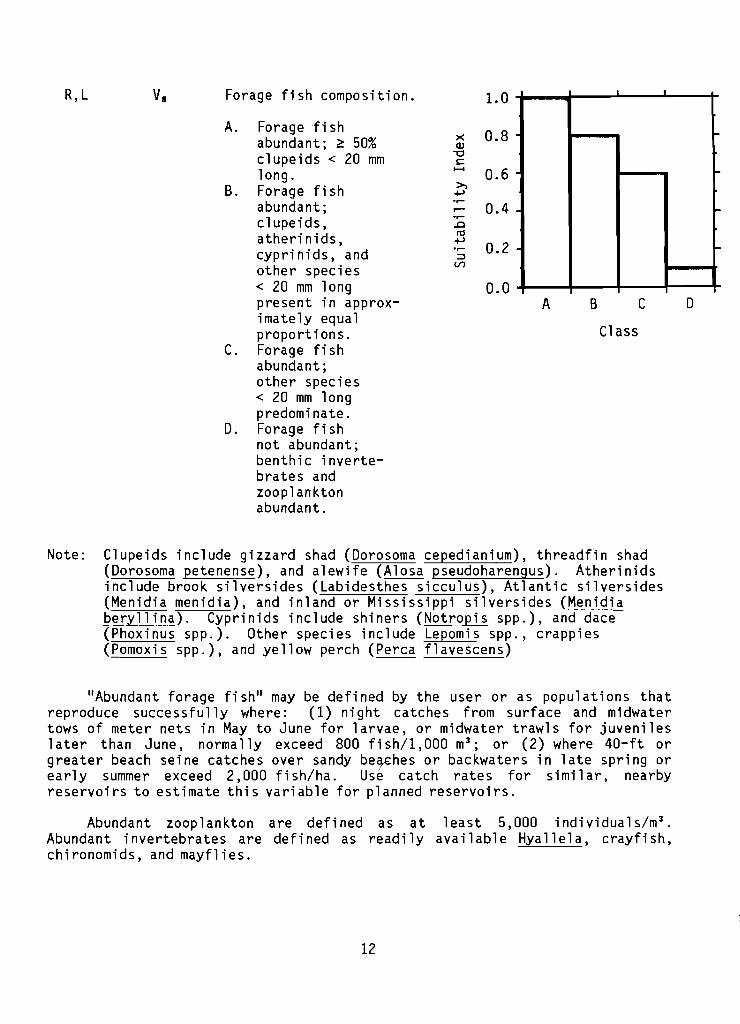
R,L v. Forage fish composition. 1.0

A. Foragefi sh0.8abundant; 2: 50% ><

OJ

clupeids < 20 mm "'0t:

long. ...... 0.6B. Forage fish >,

+->abundant; ...... 0.4clupeids, .0

atherinids, rtl+-> 0.2cyprinids, and.....

:::::l

other species V>

< 20 mm long 0.0present in approx-imately equalproportions.

C. Forage fishabundant;other species< 20 mm longpredominate.

D. Forage fi shnot abundant;benthic inverte-brates andzooplanktonabundant.

A B C

Class

o

Note: Clupeids include gizzard shad (Dorosoma cepedianium), threadfin shad(Dorosoma petenense), and alewife (Alosa pseudoharengus). Atherinidsinclude brook silversides (Labidesthes sicculus), Atlantic silversides(Menidia menidia), and inland or Mississippi silversides (Menidiaberyllina). Cyprinids include shiners (Notropis spp.), and dace(Phoxinus spp.). Other species include Lepomis spp., crappies(Pomoxis spp.), and yellow perch (Perea flavescens)

"Abundant forage fish" may be defined by the user or as populations thatreproduce successfully where: (1) night catches from surface and midwatertows of meter nets in May to June for larvae, or midwater trawls for juvenileslater than June, normally exceed 800 fishll,OOO m"; or (2) where 40-ft orgreater beach seine catches over sandy be~hes or backwaters in late spring orearly summer exceed 2,000 fish/ha. Use catch rates for similar, nearbyreservoirs to estimate this variable for planned reservoirs.

Abundant zooplankton are defined as at least 5,000 individuals/m 3•

Abundant invertebrates are defined as readily available Hyallela, crayfish,chironomids, and mayflies.

12

.....

1.0

~ 0.6

0.2

0.4

0.0

.....

..cto

.j..l

x~ 0.8s::......

.....

.....

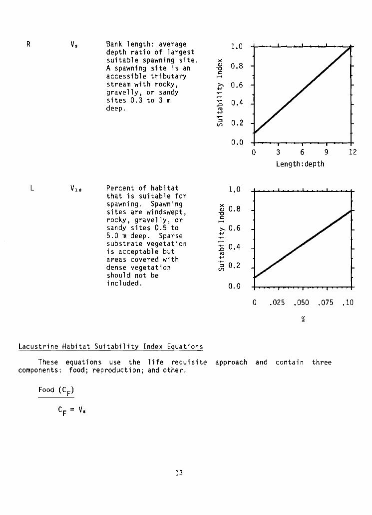
Bank length: averagedepth ratio of largestsuitable spawning site.A spawning site is anaccessible tributarystream with rocky,gravelly, or sandysites 0.3 to 3 mdeep.

VgR

o 369Length:depth

12

L Percent of habitatthat is suitable forspawning. Spawningsites are windswept,rocky, gravelly, orsandy sites 0.5 to5.0 m deep. Sparsesubstrate vegetationis acceptable butareas covered withdense vegetationshould not beincluded.

1,0

xQ) 0.8

\::ls::......>, 0.6

.j..l

.....:c 0.4to-+-'.....:::3 0.2

V)

0.0

o .025 .050 .075 .10

%

Lacustrine Habitat Suitability Index Equations

These equations use the life requisite approach and contain threecomponents: food; reproduction; and other.

13

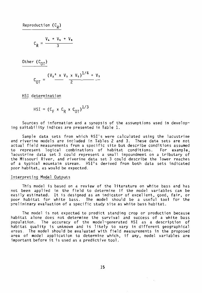
Reproduction (CR)

C = -----;0----R 3

if no suitable tributary streams are accessibleduring spawning season.

When suitable tributary streams are accessible during spawning,

V4 + V6 + Vg + Vl D

CR = the highest of -------=-4-----

or the above equation.

Other (COT)

1/3(V l

2 x Vs ) + V7

COT = 2

HSI determination

if CF, CR, or COT ~ 0.4, the HSI equals the lowest value of CF, CR, orCor

Riverine Habitat Suitability Index Equations

These equations use the life requisites approach and contain food,reproduction, and other components.

14

Reproduction (CR)

(V 2 V x Vs)I/4 + V72 X 3

2COT = ----;;;------

HSI determination

HSI

Sources of information and a synopsis of the assumptions used in develop­ing suitability indices are presented in Table 1.

Sample data sets from which HSlis were calculated using the lacustrineand riverine models are included in Tables 2 and 3. These data sets are notactual field measurements from a specific site but describe conditions assumedto represent logical combinations of habitat conditions. For example,lacustrine data set 3 could represent a small impoundment on a tributary ofthe Missouri River, and riverine data set 3 could describe the lower reachesof a typical mountain stream. HSI I S derived from both data sets indicatedpoor habitat, as would be expected.

Interpreting Model Outputs

This model is based on a review of the literature on white bass and hasnot been applied in the field to determine if the model variables can beeasily estimated. It is designed as an indicator of excellent, good, fair, orpoor habitat for white bass. The model should be a useful tool for thepreliminary evaluation of a specific study site as white bass habitat.

The model is not expected to predict standing crop or production becausehabitat alone does not determine the survival and success of a white basspopulation. The accuracy of the model-generated HSI as a description ofhabitat quality is unknown and is likely to vary in different geographicalareas. The model should be evaluated with field measurements in the proposedarea of model application to determine which, if any, model variables areimportant before it is used as a predictive tool.

15

Table 1. Data sources and assumptions for white bass suitabilityindices. "Excel l ent" habitat for white bass was assumed tocorrespond to an SI of 0.8 to 1. 0, "qood" habi tat to an SI of0.6 to 0.8, lIfairll habitat to an SI of 0.4 to 0.6, and "poorllhabitat to an SI of 0 to 0.4.

Variable

V,.

Assumptions and sources

White bass populations do poorly in lakes or reservoirssmaller than 400 acres (162 ha) (Jenkins and Elkin 1957),but are successful in large bodies of water when food andspawning requirements are met (Riggs 1955).

The native range of white bass includes the large rivers ofthe Great Lakes and Mississippi drainages (Van Oosten 1942;Sigler 1949b). Although white bass may be associated withlow order streams during spawning migrations, they commonlyinhabit large rivers. Where their range has been extendedby reservoir stocking, white bass have become establishedin larger rivers, such as the Missouri River in Missouri(Pflieger 1975), or in the tailwaters of large reservoirs(Walburg et al. 1971). Rivers from which large populationsof resident white bass have been repurted are stream order 9or greater. Stream orders 4 and below are considered pooryear around habitat because white bass are found in suchlower order streams only during spawning.

Riverine white bass are not found in the mainstream butfrequent areas where natural or man-made structures slowthe current (Gammon 1973; Kallemeyn and Novotny 1977;Pennington et al. 1983). Adult white bass apparently with­stand velocities ~ 1 m/sec, but low velocity areas arenecessary for forage fish survival and as nursery areas forlarval bass (Beckman and Elrod 1971; Storck et al. 1978).Based on our best judgement, a habitat in which at least 25%of the area is low-velocity should provide sufficient nurseryor feeding sites. A riverine habitat in which more than 75%of its area is low-velocity is atypical of rivers where whitebass are abundant.

White bass spawn at depths of 0.5 to 6.0 m, and the demersaleggs develop while attached to the substrate. A decrease inwater level that exposes the eggs results in embryo mortality.The effect on white bass year class strength depends on theextent and rapidity of the decrease at the spawning site.Water level reductions can indirectly affect white basssurvival and growth when developing forage fish embryos areexposed and die (Martin et al. 1981). Because forage fish

16

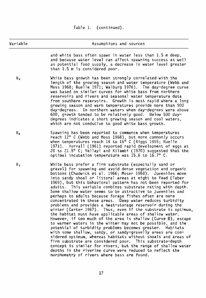
Table 1. (continued).

Variable Assumptions and sources

and white bass often spawn in water less than 1.5 m deep,and because water level can affect spawning success as wellas potential food supply, a decrease in water level greaterthan 1.5 m is considered poor.

White bass growth has been strongly correlated with thelength of the growing season and water temperature (Webb andMoss 1968; Ruelle 1971; Walburg 1976). The day-degree curvewas based on similar curves for white bass from northernreservoirs and rivers and seasonal water temperature datafrom southern reservoirs. Growth is most rapid where a longgrowing season and warm temperatures provide more than 900day-degrees. In northern waters when day-degrees were above600, growth tended to be relatively good. Below 500 day­degrees indicates a short growing season and cool waters,which are not conducive to good white bass growth.

Spawning has been reported to commence when temperaturesreach 12° C (Webb and Moss 1968), but more commonly occurswhen temperatures reach 14 to 16° C (Riggs 1955; Ruelle1971). Horrall (1961) reported rapid development of eggs at20 to 21.5° C; Yellayi and Kilambi (1970) suggested that theoptimal incubation temperature was 15.6 to 16.7° C.

V7 White bass prefer a firm substrate (especially sand orgravel) for spawning and avoid dense vegetation and organicbottoms (Chadwick et al. 1966; Moser 1968). Juveniles moveinto sandy shoal or littoral areas at night to feed (Taber1969), but this behavioral pattern has not been reported foradults. This variable combines substrate rating with depth.Some shallow water seems to be attractive to juveniles andperhaps to adults because forage fishes often are moreconcentrated in these areas. Deep water reduces turbidityproblems and provides a heat-storage reservoir during thewinter (Carter 1967). Thus, even if the substrate is optimum,the habitat must have applicable areas of shallow water.However, if too much of the area is shallow (Curve B), escapeto warmer waters in the winter may not be possible, and thepotential of turbidity problems becomes greater. Habitatswith some shallow, sandy, or sandy-gravelly areas are con­sidered optimum, whereas habitats without shoals and areas offirm substrate are considered poor. This substrate-depthconcept is similar for rivers, but the range of shallow waterdepths in the riverine curve were reduced to reflect themorphometry of rivers where bass are found.

17

Table 1. (concluded).

Variable Assumptions and sources

Vigorous white bass populations have been more closelyrelated to abundant forage fish populations than anyother variable (Jenkins and Elkin 1957; Houser and Bryant1970; Pflieger 1975). Shad are the preferred forage wherethey are available, but larval atherinids, centrarchids,and cyprinids are also good forage (Sigler 1949b; Olmstedand Kilambi 1971; Walburg et al. 1971). Although theygenerally are piscivorous, white bass are opportunisticand forage on invertebrates and zooplankton when they areplentiful (Sigler 1949b; Bonn 1953; McNaught and Hasler1961; Olmsted and Kilambi 1971).

When a stream tributary to a reservoir or river used byadult bass is accessible, it will probably be used forspawning (Riggs 1955). Firm substrates at depths of 0.3 to3.0 m are preferred sites (Riggs 1955; Webb and Moss 1968;Becker 1983), and one or two sites are used by the entirepopulation. It is important that the eggs sink onto a suit­able substrate. The length of the spawning site must increase(or velocity decrease) as depth increases so that the eggssink before being swept away by the current. The assignmentof an SI to different length:depth ratios was based on theauthors' judgement of the probable sinking rate for the eggs,typical spawning stream velocity and depth, and the congregat­ing spawning behavior of white bass.

Lake spawning sites are commonly used successfully. However,white bass prefer running water, so a lake site will never beassigned an SI of 1.0. A relatively small area is requiredfor spawning because white bass spawn as a group at one siterather than make individual nests (Riggs 1955). This curvewas constructed subjectively and should be adjusted if localconditions suggest a different relationship.

18

Table 2. Sample data sets using lacustrine HS1 model.

Data set 1 Data set 2 Data set 3

Variable Data S1 Data S1 Data S1

Surface area Vi 25,000 1.00 10,000 1. 00 250 0.50

Water levelchange V4 -0.5 0.70 -1.0 0.50 -1.0 0.50

Day-degrees Vs 900 1.00 750 0.80 500 0.60

Temperature Vf, 16 0.80 16 0.80 14 0.40

Substrate V7 75% sand 1. 00 25% gravel 0.30 25% gravel 0.3025'~ gravel 75% silt/mud 75% si ItCurve C Curve C Curve B

Forage fi sh Va abundant 1.00 abundant 1. 00 centrar- 0.60clupeids clupeids chid

larvae

% spawning VlO 0.10% 0.80 0.07% 0.60 0.07% 0.60habitat

Component S1

CF = 1.00 1. 00 0.60

CR = 0.76 0.63 0.50

COT = 1.00 0.61 0.42

HS1 = 0.91 0.72 0.50

19

Table 3. Sample data sets using riverine HS1 model.

Data set 1 Data set 2 Data set 3

Variable Data S1 Data S1 Data S1

Stream order V2 10 1. 00 7 0.70 3 0.30

% slowvelocity V3 50 1.00 20 0.80 10 0.50

Water levelchange V4 0 1.00 -0.5 0.70 -1. 0 0.50

Day-degrees Vs 750 0.80 500 0.60 250 0.10

Temperature VG 16 0.80 14 0.40 12 0.20

Substrate V7 50% sand 0.80 50% gravel 0.60 50% gravel 0.50type 25% gravel 25% sand 50% boulder

25% silt 25% silt Curve ACurve C Curve B

Spawning siteLength:depthratio Vg 12 1. 00 6 0.50 6 0.50

Forage fish Va centrarchids 0.80 centrarchids 0.60 inverte- 0.30clupeids brates

Component S1

CF = 0.80 0.60 0.10

CR = 0.93 0.53 0.40

COT = 0.87 0.65 0.48

HS1 = 0.86 0.59 0.27

20

ADDITIONAL HABITAT MODELS

Mode 1 1

Optimal lacustrine habitat for white bass is characterized by a large(> 800 ha) surface area; sandy 1ittora 1 and shoa1 areas coveri ng 10 to 30% ofthe total habitat; long, warm summers (2: 900 degree-days); an accessibletributary stream with rocky or gravelly substrate; and an abundant clupeidpopulation of small individuals.

HSI = number of above criteria present5

Model 2

Optimal riverine habitat for white bass is characterized by high orderrivers; low velocity (~ 0.4 m/sec) areas, such as deep pools, protected sitesdownstream of dikes or other structures, backwaters, or stream margins; acces­sible tributary streams with a rocky or gravelly substrate; long, warm summers(2: 900 day-degrees); and an abundant clupeid population of small individuals.

HSI = number of above criteria present5

INSTREAM FLOW INCREMENTAL METHODOLOGY (IFIM)

The U.S. Fish and Wildlife Service's Instream Flow Incremental Methodology(IFIM), as outlined by Bovee (1982), is a set of ideas used to assess instreamflow problems. The Physical Habitat Simulation System (PHABSIM), described byMi"1 hous et a1. (1984), is one component of I FIM that can be used by i nves­tigators interested in determining the amount of available instream habitatfor a fi sh speci es as a function of streamflow. The output generated byPHABSIM can be used for several IFIM habitat display and interpretationtechniques, including:

1. Optimization. Determination of monthly flows that minimize habitatreductions for species and life stages of interest;

2. Habitat Time Series. Determination of the impact of a project onhabitat by imposing project operation curves over historical flowrecords and integrating the difference between the curves; and

3. Effective Habitat Time Series. Calculation of the habitat require­ments of each life stage of a fish species at a given time by usinghabitat ratios (relative spatial requirements of various lifestages).

21

Suitability Index Graphs as Used in IFIM

PHABSIM utilizes Suitability Index graphs (SI curves) that describe theinstream suitability of the habitat variables most closely related to streamhydraulics and channel structure (velocity, depth, substrate, temperature, andcover) for each major life stage of a given fish species (spawning, egg incuba­tion, fry, juvenile, and adult). The specific curves required for a PHABSIManalysis represent the hydraulic-related parameters for which a species orlife stage demonstrates a strong preference (i.e., a species that only showspreferences for velocity and temperature will have very broad curves fordepth, substrate, and cover).

Terminology pertaining to four categories of SI curves is describedbelow. All species curves for use with HEP and IFIM are referred to collec­tively as suitability index (SI) curves or graphs. The designation of a curveas belonging to a particular category does not imply that there are differencesin the quality or accuracy of curves among the four categories.

Category one curves are the most common type presently available for usewith HEP or IFIM. Category one curves usually have, as their basis, one ormore literature sources. Some SI curves may be derived from general statementsmade in the 1iterature about fi shes (i. e., ra i nbow trout spawn in grave 1; fryprefer shallow water). Some category one curves may come from 1iteraturesources, which include variable amounts of field data (i .e., from a sample sizeof 300, fry were observed in velocities ranging 0.0 to 3.0 fUsec, and 80%were found in velocities less than 1.0 ft/sec). Other category one curves maybe based entirely on professional opinion, by using the Delphi technique oreducated guesswork (i .e., an expert believes that velocities ranging 1.0 to8.0 fUsec are necessary for successful spawning of striped bass). Mostcategory one curves are the result of a combination of sources; the finalcurve may include information from the literature, combined with field data,and smoothed or modified using professional judgement. Category one curvesusua lly are intended to refl ect genera 1 habi tat sui tabi 1i ty throughout theentire geographic range of the species and throughout the year, unless theyare identified as being applicable only to a given area or season. In thelatter case, curves developed for a specific area or stream may not accuratelyreflect habitat utilization in other areas. Curves meant to describe thegeneral habitat suitability of a variable throughout the entire range of aspecies may not be as sensitive to small changes of the variable within aspecific stream (i .e., rainbow trout generally utilize silt, sand, gravel, andcobble for spawning substrate, but utilize only cobble in Willow Creek,Colorado).

Category two curves are derived from frequency analyses of field data andbasically are curves fit to a frequency histogram. Each curve describes theobserved utilization of a habitat variable by a life stage. Category twocurves, unaltered by professional judgment or other sources of information,are referred to as utilization curves. When modified by judgment, they becomecategory one curves. Utilization curves from one set of data are not applic­able for all streams and situations (i .e., a depth utilization curve from ashallow stream cannot be used for the Missouri River). Category two curves,therefore, are usually biased because of limited habitat availability. An

22

ideal study stream would have all substrate and cover types present in equalamounts; all depth, velocity, and percent cover intervals available in equalproportions; and all combinations of all variables present in equal propor­tions. Utilization curves from such a perfectly designed study theoreticallyshould be transferable to any stream within the geographical range of thespecies. Curves from streams with high habitat diversity are generally moretransferable than curves from streams with low habitat diversity. Users of acategory two curve should first review the stream description to see if condi­tions were similar to those present in the stream segment to be investigated.Some variables to consider might include stream width, depth, discharge,gradient, elevation, latitude and longitude, temperature, water quality,substrate and cover diversity, fish species associations, and data collectiondescriptors (time of day, season of year, sample size, and sampling methods).If one or more of these factors deviate significantly from those at theproposed study site, curve transference is not advised, and the investigatorsshould develop their own curves.

Category three curves are derived from utilization curves that have beencorrected for envi ronmenta 1 bi as and, therefore, represent the preference ofthe species. To generate a preference curve, habitat utilization data andhabitat availability data must be simultaneously collected from the same area.Habitat availability should reflect the relative amount of different habitattypes in the same proportions as they exist throughout the stream study area.A curve is developed for the habitat frequency distribution in the same way asfor fish utilization observations, and the equation coefficients of the avail­ability curve are subtracted from the equation coefficients of the utilizationcurve, resulting in preference curve coefficients. Theoretically, categorythree curves should be unconditionally transferable to any stream, althoughthis has not been validated. At present, very few category three curves existbecause most habi tat uti 1i zat i on data sets are wi thout concomi tant habi tatavailability data sets. In the future, the need to collect habitat avail­ability data should be impressed on investigators.

Category four curves (conditional preference curves) describe habitatrequirements as a function of interaction among variables. For example, fishdepth utilization may depend on the presence or absence of cover, and velocityutilization may depend on time of day or season of year. Category four curvesare just beginning to be developed.

IFIM analyses may utilize any or all categories of curves, but categorythree and four curves should yield the most precise results. Category twocurves should yield accurate results if they are transferable to the streamsegment under investigation. If category two curves are not transferable fora particular application, category one curves may be a better choice.

For an I FIM ana ly s is of ri veri ne habi tat, an investigator may wi sh toutilize the curves available in this publication, modify the curves based onnew or additional information, or collect field data to generate new curves.For example, if an investigator has information that spawning habitat utiliza­tion in his or her study stream is different from that represented by the SI

23

curves, they may want to modify the exi st i ng SI curves or co11 ect data togenerate new curves. Once a decision has been made on the curves to be used,the curve coordinates are used to build a computer file (FISHFIL), which is anecessary component of PHABSIM analyses (Milhous et al. 1984).

Availability of Graphs for Use in IFIM

A great deal of variability in habitat requirements or preferences existsamong different populations within the range of the white bass in the UnitedStates. Some white bass populations complete their life cycles in lakes orreservoirs, some spend their 1ives in rivers, some inhabit lakes and spawn intributary streams, and some reside and spawn in lakes, but will spawn intributaries if the streamflow is above a certain level.

Little is known about the physical microhabitat requirements of riverinepopulations of white bass. Many of the available SI curves (Table 4; Figs. 3through 7) are based on studies of white bass in lentic environments, whichmayor may not be applicable to lotic environments. The SI curves availablefor IFIM analyses of white bass habitat are crude at best, and investigatorsare encouraged to develop their own curves whenever possible or modify exist­ing curves to reflect habitat utilization at their selected study sites.

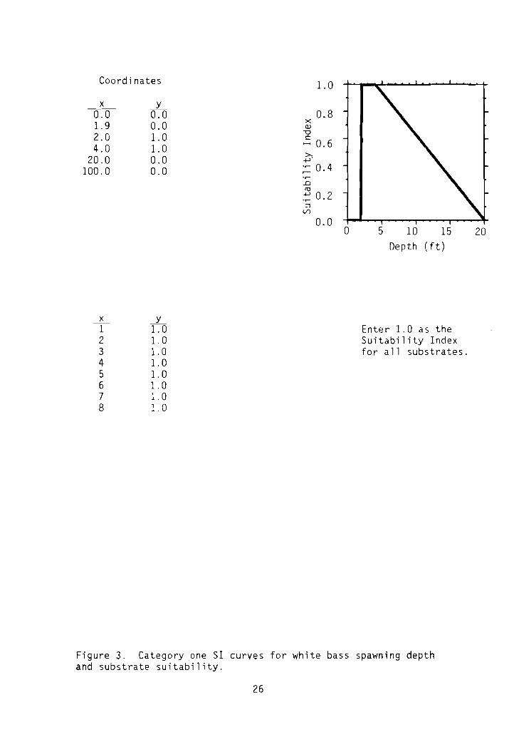
White bass spawning periods range from 5 to 25 days and generally occurbetween Apri 1 and June. Spawn i ng has been reported to occur in qui et watersof lakes, under falls, and in riffles of streams. However, not enough quanti­tative information was found to develop an SI curve for water velocity.Reported spawning depths have ranged from 2 to 20 ft in 1akes and from 2 to4 ft in streams. Females scatter eggs near the water surface, over a varietyof substrate types, including mud, silt, sand, gravel, rocks, logs, rootedplants, and algae. Spawning temperatures range from 54 to 75° F (Chadwicketal.1966).

Egg incubation requires 2 to 4 days at water temperatures ranging from 60to 71° F (Riggs 1955; Horrall 1961). Eggs are demersal and adhesive, andsuitable substrate includes gravel, cobble, boulders, logs, submerged vegeta­tion, and filamentous algae, as long as dissolved oxygen requirements are met.Water depths utilized for spawning are assumed to be suitable for egg incuba­tion. No information was found in the literature concerning velocitytolerances of incubating eggs, although velocities of zero are thought to besuitable because eggs can incubate successfully in lentic environments. Eggsthat are hidden are probably less susceptible to predation, but an SI curvefor cover is not necessary because it is assumed that suitable substratesatisfies cover requirements.

White bass are assumed to be fry at lengths less than 2.0 inches. SIcurves for velocity and depth were derived from the only source of data avail­able (n = 23), collected in the Missouri River by Kallemeyn and Novotny (1977).The upper range of the depth curve was extended based on information in Taber(1969) and Storck et al. (1978). Insufficient information was found fordeveloping a substrate curve. Fry have been collected over silt and sand(Kallemeyn and Novotny 1977), which may be more a function of velocity prefer­ences than of substrate preferences. No i nformat i on was located regardi ng

24

Table 4. Availability of SI curves for IFIM analyses of white bass habitat. a

Ve 1ocity Depth Substrate Temperature Cover

Spawning No curve Use SI curve, Use SI curve, Use SI curve No curveavailable. Fig. 3. Fig. 3. for V6 • necessary.

Egg i ncuba ti on No curve Use SI curve, Use SI curve, Use SI curve No curveavailable. Fig. 4. Fig. 4. for V6' necessary.

N Fry Use SI curve, Use SI curve, No curve Use SI curve, No curve<.TI Fig. 5. Fig. 5. available. Fig. 5. available.

Juvenil e Use SI curve, Use SI curve, No curve Use SI curve, No curveFig. 6. Fig. 6. available. Fig. 6. available.

Adult No curve Use SI curve, No curve Use SI curve, No curveavailable. Fig. 7. available. Fig. 7. available.

aWhen use of SI curves is prescribed, refer to the appropriate curve in the HSI or IFIM section.

Coordinates

x----0:0­

1.92.04.0

20.0100.0

x12345678

y0.00.01.01.00.00.0

Y1.01.01.01.01.01.01.01.0

1.0

0.8X<lJ-0

.s 0.6~;:: 0.4-r-:..0<0

.;: 0.2~

VJ

0.0a 5 10 15

Depth (ft)

Enter 1.0 as theSuitability Indexfor all substrates.

20

Figure 3. Category one SI curves for white bass spawning depthand substrate suitability.

26

Coordinates1.0

x yOT O~O 0.8

1.9 0.0 ><OJ

2.0 1.0 -0c 0.64.0 1.0

20.0 0.0 >,....,100.0 0.0 0.4

..0IU...., 0.2::::::l

Vl

0.0 a 5 10 15 20Depth (ft)

I I

X y 1.01 I~52 0.0 0.83 0.0 x4 0.0 OJ

-0 0.65 1.0 c.......

6 1.0 >,

7 1.0....,

0.48 1.0

..0IU

0.2....,::::::l

Vl

0.0 1 2 3 4 5 6 7 8

Substrate code

1 =

2 =3 =4 =5 =6 =

7 =8 =

plant detritus/organic material, logs,submerged vegetation, filamentous algaemudlsoft cl aysilt (particle size < 0.062 mm)sand (particle size 0.062-2.000 mm)gravel (particle size 2.0-64.0 mm)cobble/rubble (particle size 64.0­250.0 mm)boulder (particle size 250.0-4000.0 mm)bedrock (solid rock)

Figure 4. Category one 51 curves for white bass egg incubationdepth and substrate suitability.

27

I

1.0Coordinates

0.8 -x

x y (l)-0(fQ 1.00 c -...... 0.60.3 0.05 >,

0.7 0.05 +-J...... -1.0 0.00 0.4......100.0 0.00 .0

to+-J -...... 0.2 \::::::JV>

0.00 1 2

Velocity (ft/sec)

1.0x(l)

x ----"L -0

(fQ c 0.80.0 ......1.0 0.1 >,

+-J2.0 1.0 0.6

13.0 1.0.0

20.0 0.0 to+-J 0.4100.0 0.0::::::J

V>

0.2

0.00 5 10 15 20

Depth ( ft)

1.0 Ix Y 0.8 -(fQ 0.0 x

32.0 0.0(l)

-0

50.0 1.0 c0.6 - I-......

89.0 1.0 >,

90.0 0.0+-J

0.4 -100.0 0.0

.0to -+-J

0.2::::::J

V>

0.0 I

0 25 50 75 100

Temperature (oF)

Figure 5. Category one 51 curves for white bass fry velocity,depth, and temperature suitability.

28

Coordinates

x y0:0 1.00

1. 0 0.601. 5 0.504.0 0.254.5 0.00

100.0 0.00

1.0

x 0.8Q)

"'0t:

..... 0.6~

~ 0.4........cttl+-'...... 0.2:3

U'l

0.0 a 1 2 345

Velocity (ft/sec)

x0:0

2.04.06.07.0

11.0100.0

y0.01.01.00.40.30.20.2

1.0

x 0.8Q)

"'0t:

..... 0.6~......:;:::: 0.4..cttl+-'.; 0.2U'l

0.0a 5 10 15

Depth (f t )

20

x0:032.054.086.087.0

100.0

--'L0.00.01.01.00.00.0

1.0

x 0.8Q)

"'0

~ 0.6>,+-'

;:: 0.4........cttl+-'...... 0.2:3

U'l

0.0a 25 50 75 100

Temperature (oF)

Figure 6. 51 curves for white bass juvenile velocity and depth(category two), and temperature (category one) suitability.

29

1.0.

Coordinates

0.8 -x -'L0-:0

><0.0 Q)

"'01.0 0.0 oS 0.6 -2.0 1.0 >,

100.0 1.0 +-'

0.4 -..c<0+-' 0.2 -:::l

(/)

0.0 I I

0 5 10 15 20

Depth ( ft)

1.0

x -'L0-:0 0.0 0.832.0 0.0 ><

Q)

54.0 1.0 "'0c:::

0.686.0 1.0 ......

87.0 0.0 >,+-'

100.0 0.0 0.4..c<0+-' 0.2:::l

(/)

0.00 25 50 75 100

Temperature (oF)

Figure 7. Category one 51 curves for white bass adult depthand temperature suitability.

30

cover, and it is unknown if cover is a habitat requirement of fry. Tempera­tures preferred by young-of-year white bass have been reported to range from50 to 89° F (Coutant 1977).

Juvenil e white bass are withi n the range of 2 to 9 inches long, andjuvenile habitat is required year-round. SI curves for depth and velocitywere derived from a frequency analysis of data (n = 130) collected in theMissouri River by Kallemeyn and Novotny (1977). Juvenile substrate and coverpreferences, if they exi s t , are unknown. Temperatures preferred by juveni 1ewhite bass are assumed to be similar to those preferred by adults, which rangefrom 54 to 86° F (Coutant 1977).

White bass become sexually mature at age I or II, and adults are individ­uals over 9.0 inches in length. Insufficient information was found in theliterature to develop SI curves for velocity, substrate, or cover preferences.The SI curve for depth was based on reports that white bass reside in theepilimnion of lakes and the assumption that all depths greater than the minimumare suitable. Temperatures preferred by adults ranged from 54 to 86° F(Coutant 1977).

REFERENCES

Armour, C. L., R. J. Fisher, and J. W. Terrell. 1984. Comparison of the useof the Habitat Evaluation Procedures (HEP) and the Instream FlowIncrementa 1 Methodology (I FIM) in aquat i c ana lyses. U. S. Fi sh Wil dl .Servo FWS/OBS-84/11. 30 pp.

Becker, G. C. 1983. Fishes of Wisconsin. Univ. Wisconsin Press, Madison.1051 pp.

Beckman, L. G., and J. H. Elrod. 1971. Apparent abundance and distributionof young-of-year fishes in Lake Oahe, 1965-69. Pages 333-347 in G. E.Hall, ed. Reservoir fisheries and limnology. Am. Fish. SoC-:- Spec.Publ. 8. 511 pp.

Bonn, E. W. 1953. The food and growth of young white bass (Morone chrysops)in Lake Texoma. Trans. Am. Fish. Soc. 82:213-221.

Bovee, K. D. 1982. A guide to stream habitat analysis using the InstreamFlow Incremental Methodology. Instream Flow Inf. Pap. 12. U.S. FishWildl. Servo FWS/OBS-82/26. 248 pp.

Chadwick, H. K., C. E. von Geldern, Jr., and M. L. Johnson. 1966. Whitebass. Pages 412-422 inA. Ca1houn, ed. In 1and fi sheri es management.California Fish Game. --

Carter, N. E. 1967. Fish distribution in Keystone Reservoir in relation tophysicochemical stratification. M.S. Thesis, Oklahoma State Univ.,Stillwater. 38 pp.

31

Coutant, C. C. 1977. Compilation of temperature preference data. J. Fish.Res. Board Can. 34(5):739-746.

Cowardin, L. M., V. Carter, F. C. Golet, and E. J. LaRoe. 1979. Classifica-tion of wetlands and deepwater habitats of the United States. U.S. FishWildl. Servo FWS/OBS-79/31. 103 pp.

Forney, J. L., and C. B. Taylor. 1963. Age and growth of white bass inOneida Lake, New York. J. New York Fish Game 10:194-200.

Gammon, J. R. 1973. The effect of thermal input on the populations of fishand macroinvertebrates in the Wabash River. Purdue Univ., Water Res.Cent., Tech. Rep. 32. 106 pp.

Gasaway, C. R. 1970. Changes in the fish population in Lake Francis Case,South Dakota, during the first sixteen years of impoundment. U.S. Bur.Sport Fish. Wildl. Tech. Pap. 56. 30 pp.

Hamilton, K., and E. P. Bergersen. 1984. Methods to estimate aquatic habitatvariables. Division of Planning and Technical Services, Bureau ofReclamation, Engineering and Research Center, P.O. Box 25007, DenverFederal Center, Denver, CO. n.p.

Hasler, A. D., E. S. Gardella, R. M. Horrall, and H. F. Henderson. 1969.Open-water orientation of white bass, Roccus chrysops, as determined byultrasonic tracking methods. J. Fish. Res. Board Can. 26:2173-2192.

two spawning populations of thein Lake Mendota, Wisconsin, withPh.D. Thesis, Univ. Wisconsin,

H0 rrall, R. M. 1961. A comparat i ve study 0 fwhite bass, Roccus chrysops (Rafinesque)special reference to homing behavior.Madison. 229 pp.

Houser, A., and H. E. Bryant. 1970. Age, growth,maturity of white bass in Bull Shoals Reservoir.Wildl. Tech. Pap. 49. 11 pp.

sex composition, andU.S. Bur. Sport Fish.

Howell, H. H. 1945. The white bass in TVA waters. J. Tenn. Acad. Sci.20:41-48.

Hynes, H. B. N. 1970. The ecology of running waters. Univ. Toronto Press,Canada. 555 pp.

Jenkins, R. M., and R. E. Elkin. 1957.Oklahoma Fish. Res. Lab., Norman, OK.

Growth of whi te bass in Oklahoma.Rep. 60. 21 pp.

Jenkins, R. M., and D. 1. Morais. 1971. Reservoir sport fishing effort andharvest in relation to environmental variables. Pages 371-384 in G. E.Hall, ed. Reservoir fisheries and limnology. Am. Fish. Soc~ Spec.Publ. 8. 511 pp.

32

Jester, D. B. 1971. Effects of commercial fishing, species introductions,and drawdown control on fish populations in Elephant Butte Reservoir, NewMexico. Pages 265-285 in G. E. Hall, ed. Reservoir fisheries andlimnology. Am. Fish. Soc.Spec. Publ. 8. 511 pp.

Ka11emeyn, L. W., and J. F. Novotny. 1977. Fish and fish food organisms invarious habitats of the Missouri River in South Dakota, Nebraska, andIowa. U.S. Fish Wildl. Servo FWS/OBS-77/25. 100 pp.

Kohler, C. C., and J. J. Ney. 1981. Consequences of an alewife die-off tofish and zooplankton in a reservoir. Trans. Am. Fish. Soc. 110:360-369.

Luebke, R. W. 1984. Personal communication. Texas Parks and WildlifeDepartment. Heart of the Hi 11 s Fi sheri es Research Station. JunctionStar Route, Box 62, Ingram, TX 78025.

Martin, D. B., L. J. Mengel, J. F. Novotny, and C. H. Walburg. 1981. Springand summer water levels in a Missouri River reservoir: effects on age-Ofish and zooplankton. Trans. Am. Fish. Soc. 110:370-381.

McCarraher, D. B., M. L. Madsen, and R. E.management of McConaughy Reservoi r ,Ha 11, ed. Reservoi r fi sheri es andPubl. 8. 511 pp.

Thomas. 1971. Ecology and fisheryNebraska. Pages 229-311 in G. E.limnology. Am. Fish. SoZ Spec.

McNaught, D. C., and A. D. Hasler. 1961. Surface school ing and feedingbehavior in the white bass, Roccus chrysops (Rafinesque), in Lake Mendota.Limnol. Oceanogr. 6:53-60.

Milhous, R. T., D. L. Wegner, and T. Waddle. 1984. User's guide to thePhysical Habitat Simulation System. Instream Flow Information Paper 11.U.S. Fish Wildl. Servo FWS/OBS-81/43 Revised. n.p.

Moser, B. B. 1968. Food habits of the white bass in Lake Texoma with specialreference to the threadfin shad. M.S. Thesis, Univ. Oklahoma, Norman.109 pp.

Mount, D. I. 1961. Development of a system for contro 11 i ng di sso1ved-oxygencontent of water. Trans. Am. Fish. Soc. 90:323-327.

Nelson, W. R. 1974. Age, growth, and maturity of thirteen species of fishfrom Lake Oahe during the early years of impoundment, 1963-68. U.S. FishWildl. Servo Tech. Pap. 77. 17 pp.

1980. Ecology of larval fishes in Lake Oahe, South Dakota.U.S. Fish Wildl. Servo Tech. Pap. 101. 18 pp.

Olmsted, L. L., and R. V. Kilambi. 1971. Interrelationships between environ­mental factors and feeding biology of white bass of Beaver Reservoir,Arkansas. Pages 397-409 in G. Hall, ed. Reservoir fisheries andlimnology. Am. Fish Soc. Spe~ Publ. 8. 511 pp.

33

Pennington, C. H., J. A. Baker, and C. L. Bond. 1983. Fishes of selectedaquatic habitats on the lower Mississippi River. U.S. Army Eng. WaterwaysExp. Stn. Tech. Rep. E-83-2. 96 pp.

Pflieger, W. L. 1975. The fishes of Missouri. Missouri Dept. Conserv.343 pp.

Priegel, G. R. 1971. Age and rate of growth of the white bass in LakeWinnebago, Wisconsin. Trans. Am. Fish. Soc. 567-569.

Riggs, C. D. 1955. Reproduction of the white bass, Morone chrysops. Invest.Indiana Lakes and Streams 4(3):87-110.

Ruelle, R. 1971. Factors influencing growth of white bass in Lewis and ClarkLake. Pages 411-424 in G. Hall, ed. Reservoir fisheries and limnology.Am. Fish. Soc. Spec. Publ. 8. 511 pp.

Siefert, R. E., A. R. Carlson, and L. S. Herman. 1974. Effects of reducedoxygen concentration on the early 1i fe stages of mountain whi tefi sh,smallmouth bass, and white bass. Prog. Fish-Cult. 36:186-191.

Si gl er, W. F. 1949a . Life hi story of the white bass in Storm Lake, Iowa.Iowa State Coll. J. Sci. 23:311-316.

1949b.(Rafinesque), ofBull. 366:203-244.

Li fe hi story of the whiteSpirit Lake, Iowa. Iowa

bass,Agr.

Lepibema chrysopsExp. Stn. Res.

Storck, T. W., D. W. Dufford, and K. T. Clement. 1978. The distribution oflimnetic fish larvae in a flood control reservoir in central Illinois.Trans. Am. Fish. Soc. 107:419-424.

Summerfelt, R. C. 1971. Factors influencing the horizontal distribution ofseveral fishes in an Oklahoma reservoir. Pages 425-439 l!! G. E. Hall,ed. Reservoir fisheries and limnology. Am. Fish. Soc. Spec. Publ. 8.511 pp.

Taber, C. A. 1969. The distribution and identification of larval fishes inthe Buncombe Creek arm of Lake Texoma with observations on spawninghabits and relative abundance. Ph.D. Thesis, Univ. Oklahoma, Norman.120 pp.

Terrell, J. W., T. E. McMahon, P. D. Inskip, R. F. Raleigh, and K. L.Williamson. 1982. Habitat suitability index models: Appendix A.Guidelines for riverine and lacustrine applications of fish HSI modelswith the Habitat Evaluation Procedures. U.S. Fish Wildl. ServoFWS/OBS-82/10.A. 54 pp.

Thompson, W. H. 1951. The age and growth of white bass, Lepi bema chrysops(Rafinesque), Lake Overholser and Lake Hefner, Oklahoma. Proc. OklahomaAcad. Sci. 30:101-110.

34

Tompkins, W. A., and M. M. Peters. 1951. The age and growth of the whitebass Lepibema chrysops of Herrington Lake, Kentucky. Kentucky Div. GameFish, Fish. Bull. 8. 12 pp.

U.S. Environmental Protection Agency. 1976. Quality criteria for water.U.S. Environ. Protection Agency, Washington, DC. 256 pp.

U.S. Fish and Wildlife Service. 1981. Standards for the development ofhabitat suitability index models. 103 ESM. U.S. Fish Wildl. Serv., Div.Ecol. Servo n.p.

Van Oosten, J. 1942. The age and growth of the Lake Erie white bass, Lepibemachrysops (Rafinesque). Pap. Michigan Acad. Sci., Arts and Letters27:307-334.

Voigtlander, C. W., and T. E. Wissing. 1974. Food habits of young andyearling white bass, Morone chrysops (Rafinesque), in Lake Mendota,Wisconsin. Trans. Am. Fish. Soc. 103:25-31.

Walburg, C. H. 1971. Loss of young fish in reservoir discharge and year-classsurvival, Lewis and Clark Lake, Missouri River. Pages 441-448 in G. E.Hall, ed. Reservoir fisheries and limnology. Am. Fish. Soc--:- Spec.Publ.8. 511 pp.

1976. Changes in the fish population of Lewis and Clark Lake,1956-74, and their relation to water management and the environment.U.S. Fish Wildl. Servo Res. Rep. 79. 33 pp.

1977. Lake Franci s case, a Mi ssouri Ri ver reservoi r: Changesin the fish population in 1954-75, and suggestions for management. U.S.Fish Wildl. Servo Tech. Pap. 95. 12 pp.

Walburg, C. H., G. L. Kaiser, and P. L. Hudson. 1971. Lewis and Clark Laketailwater biota and some relations of the tailwater and reservoir fishpopulations. Pages 449-467 in G. E. Hall, ed. Reservoir fisheries andlimnology. Am. Fish. Soc. Spe~ Publ. 8. 511 pp.

Ward, H. C. 1949. A study of fish populations, with special reference to thewhite bass, Lepi bema chrysops (Rafi nesque), in Lake Duncan, Oklahoma.Proc. Oklahoma Acad. Sci. 30:69-84.

Webb, J. F., and D. D. Moss. 1968. Spawning behavior and age and growth ofwhite bass in Center Hill Reservoir, Tennessee. Proc. Southeast. Assoc.Game Fish Comm. 21:443-457.

Yellayi, R. R., and R. V. Kilambi. 1970. Observations on early developmentof white bass, Roccus chrysops (Rafinesque). Proc. Southeast. Assoc.Game Fish Comm. 23:261-265.

35

50272 ., 01

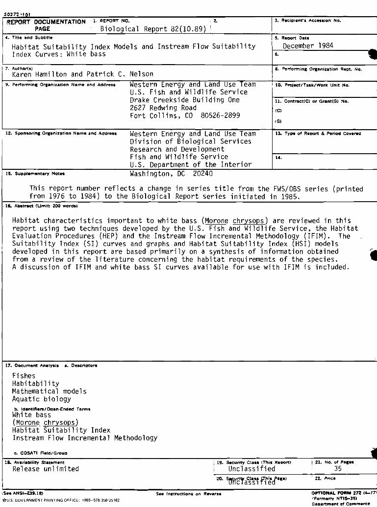
developed ln thlS report are based prlmarlly on a synthesls of lnformatlon obtalnedfrom a review of the literature concerning the habitat requirements of the species.A discussion of IFIM and white bass SI curves available for use with IFIM is included.

REPORT DOCUMENTATION 1. REPORT NO. 2. ! 3. Recipient's Accession No.I

PAGE Biological Report 82(lO.89) !

4. Title and Subtitle 5. Reoort Date

Habitat Suitability Index Models and Instream Flow Suitability December 1984Index Curves: White bass 6.

~7. Author(s) 8. i>erlorminc O,..anization Rept. No.

Karen Hamilton and Patrick C. Nelson~. Performinc Orc.nization Name and Address Western Energy and Land Use Team , 10. Project/Task/Worle Unit No.

U.S. Fish and Wildlife ServiceDrake Creekside Building One 11. Contract(C) or Gr.nt(G) No.

2627 Redwing Road (ClFort Collins, CO 80526-2899

(G)

12. Soonsorin. O....nization N.me and Addre.s Western Energy and Land Use Team 13. Type of Reoort & Period Covered

I

Division of Biological ServicesResearch and DevelopmentFish and Wildlife Service 14.

U.S. Department of the Interior15. Supplement.ry Not.. Washington, DC 20240

This report number reflects a change in series title from the FWS/OBS series (printedfrom 1976 to 1984) to the Biological Report series initiated in 1985 .

. 11S. Abstract (Umit: 200 word.)

Habitat characteristics important to white bass (Morone chrysops) are reviewed in thisreport using two techniques developed by the U.S. Fish and Wildlife Service, the HabitatEvaluation Procedures (HEP) and the Instream Flow Incremental Methodology (IFIM). The

ISuitability Index (SI) curves and graphs and Habitat Suitability Index (HSI) models

17. Oocument An.'ysi. a. Oescriptors

FishesHabitabilityMathematical modelsAquatic biology

b. Identlfiers/Open·Ended rerms

White bass(Morone chrysops)Habitat Suitability IndexInstream Flow Incremental Methodology

e. COSATl Field/Group

18. Avail.bility Statement

Release unlimitedi 19. Security CI.... (This ReDOrt)

Unclassified21. NO. of P....

3520. s.:lIri4' Class f"is p.ce,unclassl lea 22. Price

(s.. ANSl-Z39.18)

*U.S. GOVERNMENT PRINTING OFFICE: 1985-578-358/25162

See InstructIons on R..,erse Ot"TlONAL FOR" 272 (4-771(Formerly NTIS-35)Oeo.rtment of Comme~e

Habitat suitabil it y index mode ls and 24 981

:::~:::' sjiillll l~111111 11111 1111 1111 111 .U54 no. 82

1:l Hea<3Quarrers 01'/1510n of BIo log ic alservices Washington , DC

)( Easlern Energy and Land Use Teamt.eetcwn WV

• Naltonal Coastal Ecosystems TeamSlidell LA

• -vesre-n Energy and Land Use TeamFl Coums CO

• toc anons 01 Reg,onal Oll,ces

~-

REGION 1, ) Regional Director

U.S. Fish lind Wildlife ServiceLloyd Five Hundred Building, Suite 1692500 N.E. Multnomah StreetPortland, Oregon 97232

REGION 4Regional DirectorU.S. Fish and Wildlife ServiceRichard B. Russell Building75 Spring Street, S.W.Atlanta, Georgia 30303

,,,__r----61,-----L, J_

I • 1. ,---I I

I

REGION 2Regional DirectorU.S. Fish and Wildlife ServiceP.O. Box 1306Albuquerque. New MeXico87103

REGION 5Regional DirectorU.S. Fish and Wildlife ServiceOne Gateway CenterNewton Corner. Massachusclls 02158

REGION 7Regional DirectorU.S. Fish and Wildlife Service1011 E. Tudor RoadAnchorage. Alaska 99503

Puerto RICO and..--. .,.,,--,..

Virgin Islands

REGION 3Regional DirectorU.S. Fish and Wildlife ServiceFederal Building, Fort SnellingTwin Cities. Minnesota 551 J I

REGION 6Regional DirectorU.S. Fish and Wildlife ServiceP.O.Box 25486Denver Federal CenterDenver. Colorado 80225

DEPARTMENT OF THE INTERIORu.s. FISH AND WILDLIFE SERVICE

, ,~

.'JHH • WII.OI .I.-':

~. ~

-. .l:\. ~.

.. .,..... to . .... , - '

As the Nation's principal conservation aleney, the Department of the Interior hal respon­sibility for most of our nationally owned public lands and natural resources. This includesfostering the wisest use of our land and water resources, protecting our fish and wildlife,preserving th&environmental and culturat'values of our national parks and historical places,and providing for the enjoyment of life through outdoor recreation. The Department as·sesses our energy and mineral resources and works to assure that their development is inthe best interests of all our people. The Department also has a major responsibility forAmerican Indian reservation communities and for people who live in island territories underU.S," administration,