HABITAT COVARIATES FOR STANDARDIZING ... - billfish.org · AN EXAMPLE WITH BLUE MARLIN C.P....
24
SCRS/2018/017 Collect. Vol. Sci. Pap. ICCAT, 75(5): 916-939 (2018) 916 HABITAT COVARIATES FOR STANDARDIZING LONGLINE CPUE: AN EXAMPLE WITH BLUE MARLIN C.P. Goodyear, 1 M. Schirripa, 2 F. Forrestal, 3 M. Lauretta 3 SUMMARY Species distribution models (SDM) integrate multiple habitat features to predict spatiotemporal patterns of population relative abundance. When appropriately scaled, the predictions constitute a continuous numerical variable suitable for inclusion as a covariate in analyses intended to standardize longline CPUE. Here we evaluate methods to incorporate such data into CPUE standardizations using simulated longline catches of blue marlin (Makaira nigricans) patterned after either US or Japanese fishing. Habitat relative densities (H) were obtained from a SDM, and a habitat coefficient for each set was estimated from H using hook depths of individual gears. Standardizations used GLMs fitted to suites of covariates including either a continuous synthetic habitat variable or traditional spatial and temporal factors (area, month) to represent habitat. Overall, SDM-derived numerical variables were superior to traditional habitat factors. However, the results for the US-based data were mixed, presumably because of better statistical balance in the habitat factors. The results also show that temperature should be useful as a continuous numeric covariate for standardizing blue marlin CPUE. RÉSUMÉ Les modèles de distribution des espèces (SDM) intègrent de multiples caractéristiques de l'habitat pour prédire les schémas spatiotemporels de l'abondance relative de la population. Lorsqu'elles sont mises à l'échelle de manière appropriée, les prédictions constituent une variable numérique continue pouvant être incluse comme covariable dans les analyses visant à standardiser la CPUE palangrière. Nous évaluons ici des méthodes pour incorporer de telles données dans des standardisations de la CPUE en utilisant des captures palangrières simulées de makaire bleu (Makaira nigricans) calquées sur la pêche américaine ou japonaise. Les densités relatives de l'habitat (H) ont été obtenues à partir d'un SDM, et un coefficient d'habitat pour chaque jeu a été estimé à partir de H en utilisant la profondeur des hameçons de chaque engin. Les standardisations utilisaient des GLM ajustés à des suites de covariables incluant soit une variable d'habitat synthétique continue, soit des facteurs spatiaux et temporels traditionnels (zone, mois) pour représenter l'habitat. Dans l'ensemble, les variables numériques dérivées de SDM étaient supérieures aux facteurs traditionnels de l'habitat. Cependant, les résultats des données basées sur les États-Unis étaient mitigés, vraisemblablement en raison d'un meilleur équilibre statistique des facteurs de l'habitat. Les résultats montrent également que la température devrait être utile en tant que covariable numérique continue pour standardiser les CPUE de makaire bleu. RESUMEN Los modelos de distribución de especies (SDM) integran múltiples características del hábitat para predecir patrones espaciotemporales de la abundancia relativa de la población. Cuando están adecuadamente escalados, las predicciones constituyen una variable numérica continua adecuada para ser incluida como covariable en análisis para estandarizar la CPUE del palangre. Aquí se evalúan métodos para incorporar dichos datos en las estandarizaciones de CPUE utilizando capturas de palangre simuladas de aguja azul (Makaira nigricans) para las que se ha establecido un patrón de acuerdo con la pesca japonesa o estadounidense. Se obtuvieron densidades relativas del hábitat (H) de un SDM, y se estimó un coeficiente del hábitat 1 1214 North Lakeshore Drive, Niceville, Florida 32578, USA. [email protected] 2 NOAA Fisheries, Southeast Fisheries Center, Sustainable Fisheries Division, 75 Virginia Beach Drive, Miami, FL, 33149-1099, USA. [email protected] 3 CIMAS/RSMAS University of Miami, 4600 Rickenbacker Cwy. Miami, FL 33149. [email protected]
-
Upload
phungkhanh -
Category
Documents
-
view
213 -
download
0
Transcript of HABITAT COVARIATES FOR STANDARDIZING ... - billfish.org · AN EXAMPLE WITH BLUE MARLIN C.P....
SCRS/2018/017 Collect. Vol. Sci. Pap. ICCAT, 75(5): 916-939 (2018)
916
HABITAT COVARIATES FOR STANDARDIZING LONGLINE CPUE:
AN EXAMPLE WITH BLUE MARLIN
C.P. Goodyear,1 M. Schirripa,2 F. Forrestal,3 M. Lauretta3
SUMMARY
Species distribution models (SDM) integrate multiple habitat features to predict spatiotemporal
patterns of population relative abundance. When appropriately scaled, the predictions constitute
a continuous numerical variable suitable for inclusion as a covariate in analyses intended to
standardize longline CPUE. Here we evaluate methods to incorporate such data into CPUE
standardizations using simulated longline catches of blue marlin (Makaira nigricans) patterned
after either US or Japanese fishing. Habitat relative densities (H) were obtained from a SDM,
and a habitat coefficient for each set was estimated from H using hook depths of individual gears.
Standardizations used GLMs fitted to suites of covariates including either a continuous synthetic
habitat variable or traditional spatial and temporal factors (area, month) to represent habitat.
Overall, SDM-derived numerical variables were superior to traditional habitat factors.
However, the results for the US-based data were mixed, presumably because of better statistical
balance in the habitat factors. The results also show that temperature should be useful as a
continuous numeric covariate for standardizing blue marlin CPUE.
RÉSUMÉ
Les modèles de distribution des espèces (SDM) intègrent de multiples caractéristiques de
l'habitat pour prédire les schémas spatiotemporels de l'abondance relative de la population.
Lorsqu'elles sont mises à l'échelle de manière appropriée, les prédictions constituent une
variable numérique continue pouvant être incluse comme covariable dans les analyses visant à
standardiser la CPUE palangrière. Nous évaluons ici des méthodes pour incorporer de telles
données dans des standardisations de la CPUE en utilisant des captures palangrières simulées
de makaire bleu (Makaira nigricans) calquées sur la pêche américaine ou japonaise. Les densités
relatives de l'habitat (H) ont été obtenues à partir d'un SDM, et un coefficient d'habitat pour
chaque jeu a été estimé à partir de H en utilisant la profondeur des hameçons de chaque engin.
Les standardisations utilisaient des GLM ajustés à des suites de covariables incluant soit une
variable d'habitat synthétique continue, soit des facteurs spatiaux et temporels traditionnels
(zone, mois) pour représenter l'habitat. Dans l'ensemble, les variables numériques dérivées de
SDM étaient supérieures aux facteurs traditionnels de l'habitat. Cependant, les résultats des
données basées sur les États-Unis étaient mitigés, vraisemblablement en raison d'un meilleur
équilibre statistique des facteurs de l'habitat. Les résultats montrent également que la
température devrait être utile en tant que covariable numérique continue pour standardiser les
CPUE de makaire bleu.
RESUMEN
Los modelos de distribución de especies (SDM) integran múltiples características del hábitat
para predecir patrones espaciotemporales de la abundancia relativa de la población. Cuando
están adecuadamente escalados, las predicciones constituyen una variable numérica continua
adecuada para ser incluida como covariable en análisis para estandarizar la CPUE del
palangre. Aquí se evalúan métodos para incorporar dichos datos en las estandarizaciones de
CPUE utilizando capturas de palangre simuladas de aguja azul (Makaira nigricans) para las
que se ha establecido un patrón de acuerdo con la pesca japonesa o estadounidense. Se
obtuvieron densidades relativas del hábitat (H) de un SDM, y se estimó un coeficiente del hábitat
1 1214 North Lakeshore Drive, Niceville, Florida 32578, USA. [email protected] 2 NOAA Fisheries, Southeast Fisheries Center, Sustainable Fisheries Division, 75 Virginia Beach Drive, Miami, FL, 33149-1099, USA.
[email protected] 3 CIMAS/RSMAS University of Miami, 4600 Rickenbacker Cwy. Miami, FL 33149. [email protected]
917
para cada lance a partir de H utilizando profundidades de anzuelo de cada arte. Las
estandarizaciones utilizaron GLM ajustados a conjuntos de covariables que incluían bien una
variable de hábitat sintético continua o los tradicionales factores espaciales y temporales (área,
mes) para representar el hábitat. En total, las variables numéricas derivadas de SDM eran
superiores a los factores de hábitat tradicionales. Sin embargo, los resultados para datos
basados en Estados Unidos eran mezclados, presumiblemente a causa de un mejor equilibrio
estadístico en los factores de hábitat. Los resultados muestran también que la temperatura
debería ser útil como covariable numérica continua para estandarizar la CPUE de la aguja azul.
KEYWORDS
Blue marlin, Longline, Catchability, Gear coefficient, Habitat coefficient, Stock assessment,
CPUE Standardization, Statistics, GLM, Data simulation, Population modeling
1. Introduction
In 2015 the ICCAT Working Group on Stock Assessment Methods initiated an effort to study longline CPUE
standardization methods using simulated data (Anon 2016). Goodyear et al. (2017) modeled catchability as a joint
function of a habitat coefficient (w) and an essential gear effect (k). The method uses a species distribution model
(SDM) to quantify habitat relative densities (H) where a longline is deployed. The SDM uses environmental
variables and species habitat utilization patterns to estimate species relative abundance. The habitat coefficient is
estimated from H using probability distributions for depths fished by the hooks. Both w and H could be used as
covariates in analyses of catch rates to estimate abundance trends. Here we test the method using data simulations
patterned after the US and Japanese longline fisheries in the Atlantic and compare the relative errors of GLM
standardization results to those derived with alternative model covariates including traditional factors for area and
intra-annual habitat variability.
2. Background
Goodyear et al. (2017) separated the catchability of a single hook (𝑞ℎ) into two factors 1) a gear effect, k, and 2)
a habitat effect, H, due variations in density caused by variations in features of the environment:
𝑞ℎ = 𝑘�̅� ℎ , 1
where:
𝑞ℎ = the catchability coefficient for the hook,
k = gear coefficient, and
H̅h = the average habitat around the hook.
Since catch is an integer resulting from a series of probabilistic encounters, for a population N it is:
𝐶ℎ ≅ 𝑘�̅� ℎ𝑁. 2
The habitat coefficient, w, is the average of H̅h , for all hooks on a longline set:
𝑤 = �̅�ℎ, and 3
𝑞𝑠 = 𝑘𝑤. 4
The habitat coefficient (w) is the part of the catchability of a longline set that varies in time and space. Given
sufficient data the values of w can be estimated independent of catch.
918
The essential gear effect (k) is a constant that accounts for features affecting catch by the gear that do not include
the availability of fish in the vicinity of a hook. Features of longlines that affect k include everything that does not
affect the density of fish in the water surrounding the hooks. In contrast to w, it cannot be estimated independent
of catch.
3. Method
This study evaluates the performance of the habitat coefficient as a covariate in a GLM by comparing results of
statistical modeling to “true” values known from simulation and with several alternative covariates. The process
involves several steps:
a) Simulate population trends to serve as the “true” trends for the purpose of the study.
b) Estimate the relative distributions of blue marlin in time and space with a species distribution model.
c) Assemble a time series of longline effort similar to real fisheries
d) Simulate time series of longline catches.
e) Construct the coefficients and create input files for the GLM’s.
f) Process the GLM.
g) Compare GLM results to known “true” values.
3.1 Population time series
To ensure the trends would be biologically reasonable, the populations used for the “true” values were computed
from a fisheries simulation model (FSIM, Goodyear 2004). This approach preserves the option for including the
standardizations in a larger evaluation of the whole assessment process. The model can compute size and age
frequencies of the population and catch by sex. It also provides annual values of MSY and related statistics that
account for tends in selectivities, etc. to document the relevant benchmarks to compare with assessment model
results. Two alternatives population trajectories intended to encompass a range of reasonable possibilities were
produced. They share all biological features except that BMSY for the larger population is 3.2 times greater than
for the smaller population. The model assumed the fishery exhibited knife-edged, age-based selectivity with full
recruitment to the fishery at age 1. Growth was sexually dimorphic with parameters used in previous analyses
(e.g., Goodyear 2015). Natural mortality in the fishable population was constant at Z=0.1 for both sexes.
Recruitment was governed by a Beverton-Holt stock-recruit function with steepness equal to 0.67 and without
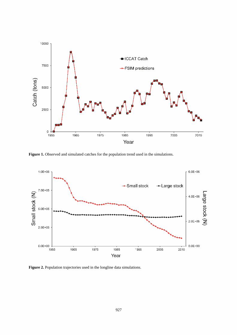
stochastic variability. Fishing mortality was set to reproduce the pattern apparent in the ICCAT Task I data from
1956 to 2016 (Figure 1). One alternative assumed MSY was within the range of observed catches which resulted
in a trajectory similar to the findings of past assessments. The population for the other alternative was assumed
to be much larger so that the historical catches are well below MSY. These population trajectories provide contrast
between alternative perspectives about the status of the stock (Figure 2).
3.2 Species distribution model
The SDM used in this study is a detailed model of the four-dimensional distribution of blue marlin (Goodyear
2016). It assumes average species density is proportional to average habitat value. The values of H are normalized
so that the sum of the products of H and the habitat layer volumes is always unity at any point in time.
Oceanographic data and species habitat utilization patterns are used to distribute the population in time and three-
dimensional space. The current implementation partitions the Atlantic from 50 S to 55 N latitude at a spatial
resolution of 1⁰ latitude and 1⁰ longitude with 46 increasingly deep layers from the surface to a maximum depth
of 1970 m. Separate distributions were computed for hours of daylight and darkness to reflect the day-night
redistribution of the species in the vertical plane. The model uses behavioral data from blue marlin PSAT tagging,
published oxygen requirements, and the time-varying distribution of these variables in oceanographic data each
month and year. The oceanographic data were monthly values from the Earth System Model from 1956 to 2012
which matched the spatial resolution of the SDM and were provided by colleagues at the US National Atlantic
Oceanographic and Meteorological Laboratory (AOML). At the time of this study 2012 was the last year that
oceanographic data were available. The 2012 values were substituted as needed to provide oceanographic data
through 2016. This convention accounts for the large month-to-month variability in oceanographic conditions but
omits any effects from annual trends that may have been important in the last few years.
919
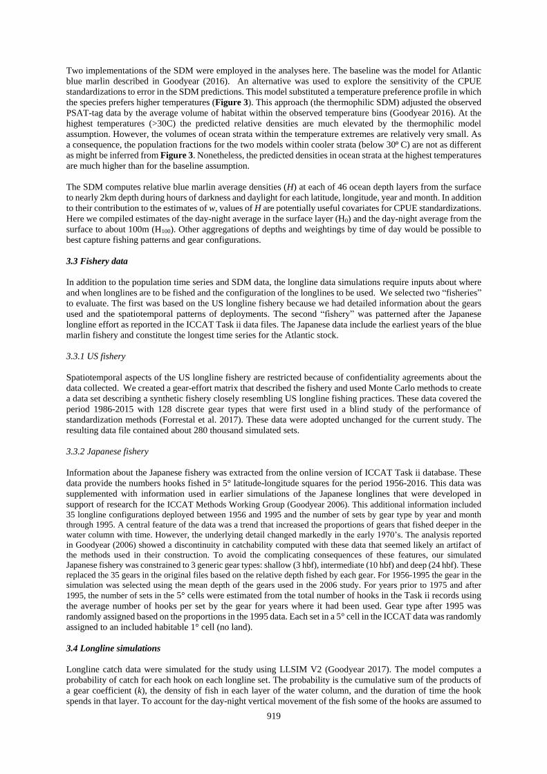
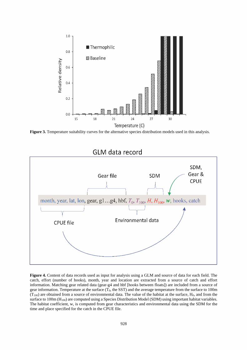
Two implementations of the SDM were employed in the analyses here. The baseline was the model for Atlantic
blue marlin described in Goodyear (2016). An alternative was used to explore the sensitivity of the CPUE
standardizations to error in the SDM predictions. This model substituted a temperature preference profile in which
the species prefers higher temperatures (Figure 3). This approach (the thermophilic SDM) adjusted the observed
PSAT-tag data by the average volume of habitat within the observed temperature bins (Goodyear 2016). At the
highest temperatures (>30C) the predicted relative densities are much elevated by the thermophilic model
assumption. However, the volumes of ocean strata within the temperature extremes are relatively very small. As
a consequence, the population fractions for the two models within cooler strata (below 30⁰ C) are not as different
as might be inferred from Figure 3. Nonetheless, the predicted densities in ocean strata at the highest temperatures
are much higher than for the baseline assumption.
The SDM computes relative blue marlin average densities (H) at each of 46 ocean depth layers from the surface
to nearly 2km depth during hours of darkness and daylight for each latitude, longitude, year and month. In addition
to their contribution to the estimates of w, values of H are potentially useful covariates for CPUE standardizations.
Here we compiled estimates of the day-night average in the surface layer (H0) and the day-night average from the
surface to about 100m (H100). Other aggregations of depths and weightings by time of day would be possible to
best capture fishing patterns and gear configurations.
3.3 Fishery data
In addition to the population time series and SDM data, the longline data simulations require inputs about where
and when longlines are to be fished and the configuration of the longlines to be used. We selected two “fisheries”
to evaluate. The first was based on the US longline fishery because we had detailed information about the gears
used and the spatiotemporal patterns of deployments. The second “fishery” was patterned after the Japanese
longline effort as reported in the ICCAT Task ii data files. The Japanese data include the earliest years of the blue
marlin fishery and constitute the longest time series for the Atlantic stock.
3.3.1 US fishery
Spatiotemporal aspects of the US longline fishery are restricted because of confidentiality agreements about the
data collected. We created a gear-effort matrix that described the fishery and used Monte Carlo methods to create
a data set describing a synthetic fishery closely resembling US longline fishing practices. These data covered the
period 1986-2015 with 128 discrete gear types that were first used in a blind study of the performance of
standardization methods (Forrestal et al. 2017). These data were adopted unchanged for the current study. The
resulting data file contained about 280 thousand simulated sets.
3.3.2 Japanese fishery
Information about the Japanese fishery was extracted from the online version of ICCAT Task ii database. These
data provide the numbers hooks fished in 5° latitude-longitude squares for the period 1956-2016. This data was
supplemented with information used in earlier simulations of the Japanese longlines that were developed in
support of research for the ICCAT Methods Working Group (Goodyear 2006). This additional information included
35 longline configurations deployed between 1956 and 1995 and the number of sets by gear type by year and month
through 1995. A central feature of the data was a trend that increased the proportions of gears that fished deeper in the
water column with time. However, the underlying detail changed markedly in the early 1970’s. The analysis reported
in Goodyear (2006) showed a discontinuity in catchability computed with these data that seemed likely an artifact of
the methods used in their construction. To avoid the complicating consequences of these features, our simulated
Japanese fishery was constrained to 3 generic gear types: shallow (3 hbf), intermediate (10 hbf) and deep (24 hbf). These
replaced the 35 gears in the original files based on the relative depth fished by each gear. For 1956-1995 the gear in the
simulation was selected using the mean depth of the gears used in the 2006 study. For years prior to 1975 and after
1995, the number of sets in the 5° cells were estimated from the total number of hooks in the Task ii records using
the average number of hooks per set by the gear for years where it had been used. Gear type after 1995 was
randomly assigned based on the proportions in the 1995 data. Each set in a 5° cell in the ICCAT data was randomly
assigned to an included habitable 1° cell (no land).
3.4 Longline simulations
Longline catch data were simulated for the study using LLSIM V2 (Goodyear 2017). The model computes a
probability of catch for each hook on each longline set. The probability is the cumulative sum of the products of
a gear coefficient (k), the density of fish in each layer of the water column, and the duration of time the hook
spends in that layer. To account for the day-night vertical movement of the fish some of the hooks are assumed to
920
fish during daylight hours and the remainder at night. The proportions are assigned for each set in an input file.
The probability of catch is entered into a Monte-Carlo procedure to test for a catch on each hook. The sum of all
outcomes determines the number of fish caught on a set. LLSIM saves data for each simulated set for subsequent
analyses. There was no additional error added to account for other factors (species misidentification, reporting,
etc.). The value of k is an input to LLSIM and read as a gear parameter. Variations in the values of k are defined
extrinsically to identify important gear features that affect the gear components of catchability. Examples include
such things as hook type, light sticks, fleet, etc. These variables are identified as important gear features in the
LLSIM input file and are saved in the output record for each catch. Each output record for a simulation provides
the month, year, latitude, longitude, identifies the gear and its features, and the number of fish caught on the set.
Though not employed here, several species can be modeled simultaneously. Our design required a minimum of 6
simulated longline datasets:
1) US fishery, small population and baseline SDM;
2) US fishery, large population and baseline SDM;
3) US fishery, small population and thermophilic SDM;
4) US fishery, large population and thermophilic SDM;
5) Japanese fishery, small population and baseline SDM;
6) Japanese fishery, large population and baseline SDM.
This design is sufficient for gross comparisons but does not provide the replication needed to characterize
precision of the alternatives.
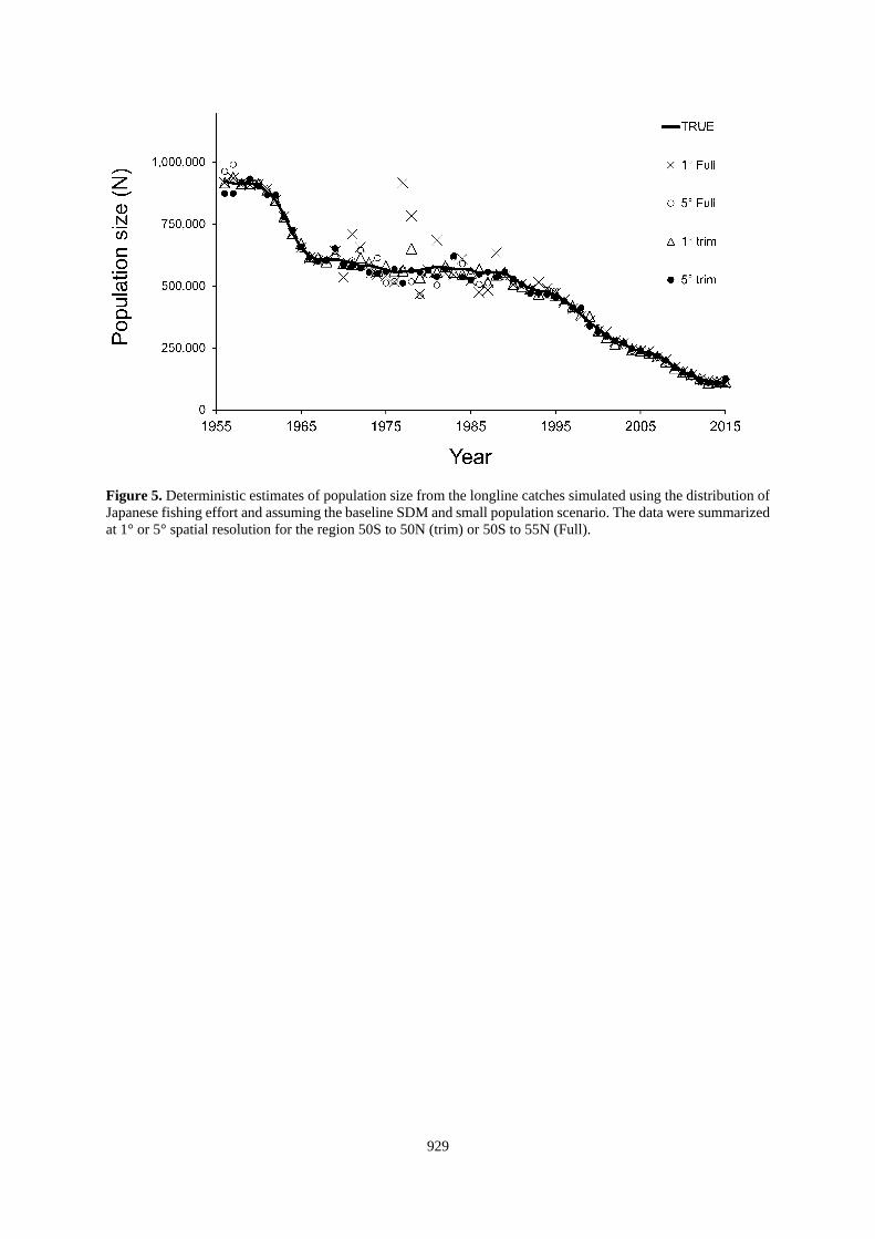
3.5 Data compilation
A pre-processing step is required to prepare a catch-effort record from the simulated logbook for use in a
standardization protocol (Figure 4). The simulated longline CPUE data are set by set observations similar to what
might be obtained from logbooks. Each record identifies the gear, month, year and location (latitude and longitude)
of the set and the numbers of blue marlin caught. The probability distributions for the hooks are input from gear
files. The species relative densities (H) at the location and time of the set are obtained from the SDM. The value
of w is then computed from the two overlapping distributions. Because of the near-surface habitat and strong
association of blue marlin with tropical conditions, temperature might be expected to be a surrogate for H. So we
also compiled the surface layer temperatures (T0) and the average from the surface to about 100m (T100) as
potential covariates.
The simulations were done at 1° resolution of latitude and longitude. However, the standardizations may be done
at the lower 5° resolution, as may be required for real data such as the Japanese example. This geometry is
accommodated by accumulating the 1° observations at the 5° resolution. In this case the temperature and H fields
are the averages of valid 1° cells within the 5° output grid and the values for w are computed from the 5° average
values of H. The program that does this task can save the result set by set to match the input records. Alternatively,
it can pool data for all sets by each gear in the 1° or 5° cell by month. The resulting data file for the simulated US
fishery were set by set. The simulated sets for the Japanese fishery were pooled to 5° x 5° to match the resolution
of the ICCAT data.
3.6 Analyses
Several GLM models were fitted to each dataset using suites of potential variables that were known to be
influential because of their roles in the simulations. The GLM’s were run in R using the glmmADMB library (R
Core Team, 2015). There was no attempt to select the variables for each fit based on any performance-based
criteria or make judgments about the quality of the fits to the simulated data. The habitat coefficients (w), habitat
relative densities (H), and temperature (C°) were included as numerical variables. Factors included year, month,
the gear (a unique id), hooks between floats (hbf), hook type, bait type, and the use of light sticks on sets. For
analyses of data patterned after the distribution of Japanese effort, the set by set data were first pooled to 5°X5°
resolution. Set by set data were used for analyses of the simulations patterned after the US longline fishery. The
standardized annual abundance predictions combined separate GLM’s for the successful sets and the catch rates
of those that were successful.
Since k is known for the gear used in the simulations, it is possible to estimate abundance for the simulated data
using the annual means of the catch/(effort*k*w) without using GLM framework. This method was applied to
each dataset to scan for anomalies and is included for reference, but it is not proffered as a reasonable option. The
GLM models for the US-based simulations included:
921
1. year, w
2. year, w, gear id
3. year, lightstick, hooktype, baittype, hbf
4. year, lightstick, hooktype, baittype, hbf, w
5. year, lightstick, hooktype, baittype, hbf, H0
6. year, lightstick, hooktype, baittype, hbf, H100
7. year, lightstick, hooktype, baittype, hbf, T0
8. year, lightstick, hooktype, baittype, hbf, T100
9. year, month, area, lightstick, hooktype, baittype, hbf
10. year, month, area, lightstick, hooktype, baittype, hbf, w
Each model was applied to each combination and reciprocal for SDM distributions assumed to be true for the
population and at the time of analysis (Table 1).
The GLM models for the simulations using the distribution of Japanese longline sets included:
1. year, w
2. year, gear id, w
3. year, hbf
4. year, hbf, w
5. year, hbf, H0
6. year, H100
7. year, hbf, T0
8. year, hbf, T100
9. year, month, area, hbf
10. year, month, area, hbf, w
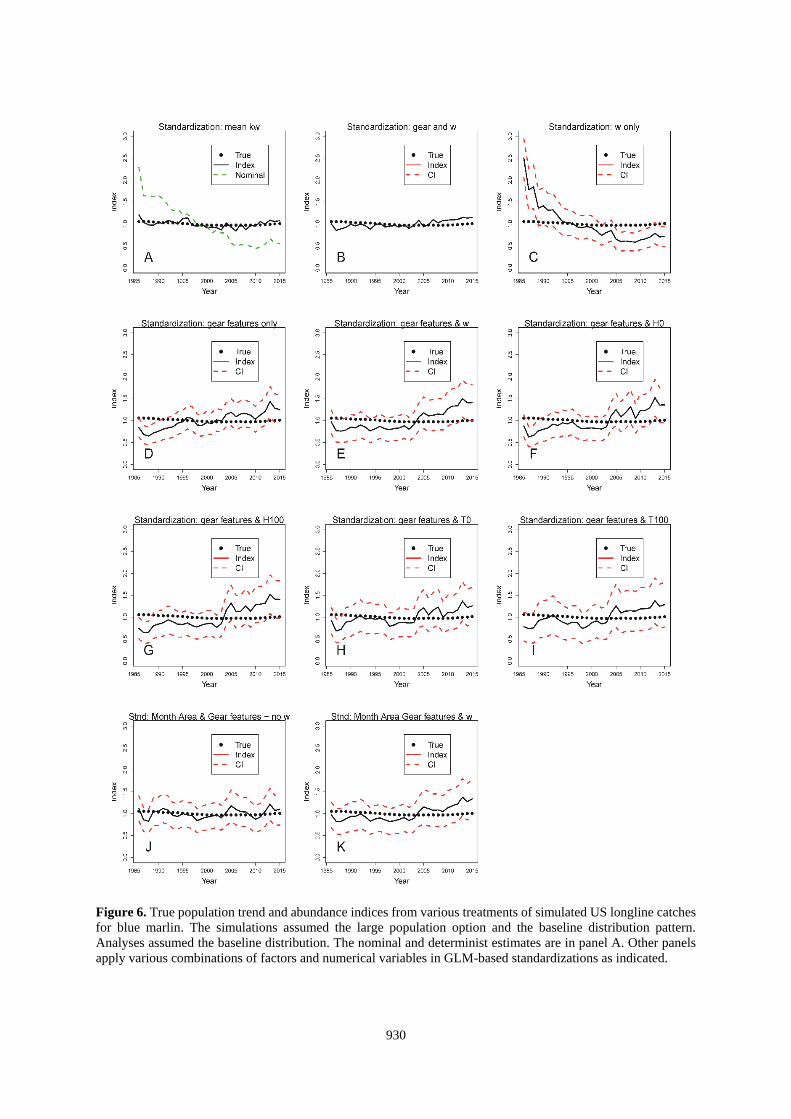
The deterministic abundance estimations possible because k was known revealed the method was sensitive to
occasional catches in marginal habitat (Figure 5), and we chose to trim about 8% of the total Japanese effort that
occurred north of 50°N or south of 50°S from further analysis. The resulting simulated CPUE data file had about
1.3 million simulated sets between 50°S and 50°N latitude. No similar adjustment was made for the simulated US
data.
The annual relative abundances for each standardization method were compared to the true values known from
the simulations. Each series was first normalized by dividing by the series mean. Error was quantified as the
difference between the predicted and true values. The sums of squares of these differences was used to compare
the relative accuracy of each standardization methods and to establish ranks among the alternatives evaluated.
Note that this use of the sum of squares is different than the standard sum of squares because the difference being
squared is measured from the true value rather than a derived statistic. Also note the CI intervals for the indices
in the plots of the standardization results in this report are based on the usual fitted statistics (without knowledge
of the true values).
4. Results
The results of each of fitting exercises for each of the simulations based on the US longline fleet are presented in
Figures 6-13. The relative error for each simulation and each standardization method are given in Table 2, along
with the rank of the average for each method. The ranks of the methods for each combination of simulation
assumption and species distribution model used to compute w and H are in Table 3. Except when the habitat
coefficient was used alone, the standardizations diminished error when compared to the nominal CPUE.
Inspections of the plots in Figures 6-13 showed that the standardization tended to correct for the downward slope
in the nominal time series that exaggerated the trend in the population. The decline in abundance was much larger
for the small population alternative. The pattern in the nominal CPUE was an aggregate effect of the transition of
fishing effort to less favorable habitat as time passed, partly by increasing use of gears that fish deeper in the water
column.
Standardizations using the deterministic calculation based on kw and that also used the correct SDM to estimate
w were both accurate and precise (Panel A of Figures 6-9 and 14-15). Results with that approach were degraded
when the choice of SDM for use in the standardization was in error (Figures 10-13, Panel A). Standardizations
that relied on the habitat coefficient alone did not improve upon the nominal for any situation evaluated here
922
(Figures 6-15, Panel C), but would be expected to mirror the results of standardizations using kw if k was constant
(e.g., 1 gear). Standardizations that used only gear features also performed poorly with respect to most other
alternatives (Tables 2-3, Figures 6-15).
The best standardizations accompanied habitat coefficients paired with factors that identified the particular gears
or also included factors for area and month with w (Tables 2-3; Figures 6-15, Panel B and K; and Figures 14-
15, Panel E). This might be a result of partitioning the data in such a manner that the GLM is able to precisely
isolate the effects of the different gears. The increased accuracy seems to come at a cost of the estimated precision
of the index. For the US-based data, including the gear id added 131 factors and increased the CI beyond the scale
of the plots (Figures 6-13, Panel B). Other standardizations also show that the CV of the estimates is not
informative about accuracy of the index (e.g., Figures 6-15, Panel C).
For the US-based datasets, the reduction in the SS averaged about 81% when w and gear id were covariates and
also when w and the gear and habitat factors were used (Table 2). Standardizations that applied other covariates
which included continuous variables (H or T) with the habitat factors (Figures 6-13, Panels E-I) reduced the total
SS by an average of between about 70 to 76%. The traditional approach using only factors to represent habitat
variability decreased the SS by 72% (Figures 6-13, Panel J; Table 3). The individual results within that matrix
did not point to a clearly superior method (Tables 2 and 3). On average, the analyses using SDM-based covariates
resulted in larger errors (SS = 1.13 vs 1.46, p=0.03, 27 df) when they were incorrectly paired with the distribution
of the population. However, the differences were smaller than the range of errors from standardizations that used
traditional month-area factors.
In contrast, the standardizations of simulation data based on the distribution of Japanese effort were substantially
improved by the inclusion of SDM-based covariates (Figures 14-15, Table 4). Each method that included gear
information as well as w reduced SS by 97-98% compared to an average of 51% (11-61%) where intra-annual
variability was modeled with factors for month and area (Table 4). Analyses that included H or temperature as
covariates were able to reduce the SS by an average of 89-98% (Table 4.) Inspections of the trends in Figures 14
and 15 suggest that the SDM-supported standardizations captured the true trend of the population much better
than the factor-based analyses, particularly when the population had declined substantially during the period.
5. Discussion
Compared to models that use factors for area and month, the accuracy of CPUE standardizations for the Japanese-
based simulated longline catch data were substantially improved by SDM-derived covariates (Table 4). The most
accurate results were obtained when the gear was identified by gear id (or hbf which was unique for each the gear
type for our simulated Japanese data). Temperature was a good surrogate for habitat relative density. The average
value in the first 100m of depth for both variables outperformed the values at the surface. The relative accuracy
of standardizations of the catch data from the US-based simulations were similar, but the differences arising from
the use of SDM-derived data or temperature were less profound. We also noted that the results were more accurate
when the SDM used to create the variable (H or w) matched the population used to simulate the catch. However,
the differences were not great.
Our results suggest that temperature is a useful covariate for standardizing CPUE when included as a continuous
numeric variable. When temperature was used as a surrogate for H, it was predictive for both the US- and
Japanese-based datasets. This is noteworthy because H is not a linear function of temperature but sharply increases
in the range of preferred temperatures. That suggests the GLMs were capable of taking advantage of whatever
empirical associations existed in the data, even when the function may depart considerably from truth. The habitat
densities (H) predicted by the baseline and thermophilic models used here are different but similarly correlated,
more so for most of the range of temperatures that constitute large ocean volumes. That feature would also be
true of other SDM parameterizations that preserve the blue marlin habitat patterns observed elsewhere (e.g.,
Goodyear 2003, Prince and Goodyear 2006, 2007, Goodyear et al. 2008, Prince et.al 2010). Consequently, it
seems likely that an SDM that satisfies reasonably established qualitative and quantitative criteria will provide
estimates of H that will outperform habitat factors depending on circumstances about factor balance. Additional
evaluations of simulated data could clarify this question.
923
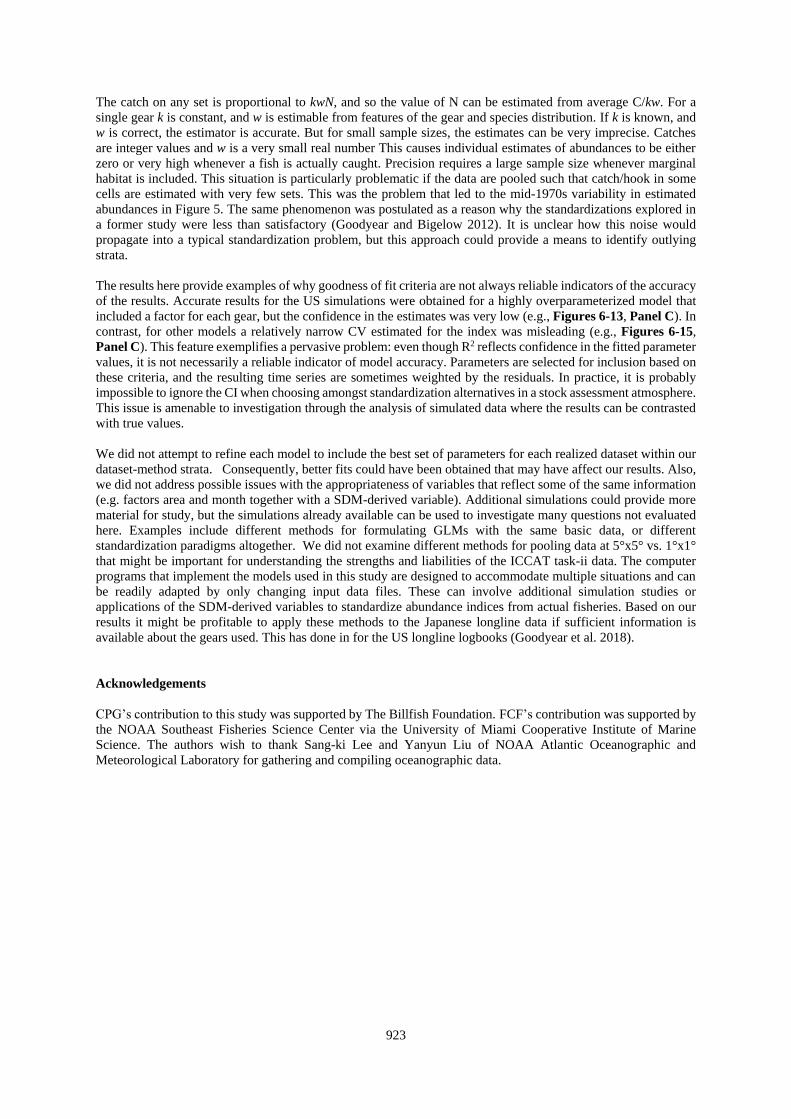
The catch on any set is proportional to kwN, and so the value of N can be estimated from average C/kw. For a
single gear k is constant, and w is estimable from features of the gear and species distribution. If k is known, and
w is correct, the estimator is accurate. But for small sample sizes, the estimates can be very imprecise. Catches
are integer values and w is a very small real number This causes individual estimates of abundances to be either
zero or very high whenever a fish is actually caught. Precision requires a large sample size whenever marginal
habitat is included. This situation is particularly problematic if the data are pooled such that catch/hook in some
cells are estimated with very few sets. This was the problem that led to the mid-1970s variability in estimated
abundances in Figure 5. The same phenomenon was postulated as a reason why the standardizations explored in
a former study were less than satisfactory (Goodyear and Bigelow 2012). It is unclear how this noise would
propagate into a typical standardization problem, but this approach could provide a means to identify outlying
strata.
The results here provide examples of why goodness of fit criteria are not always reliable indicators of the accuracy
of the results. Accurate results for the US simulations were obtained for a highly overparameterized model that
included a factor for each gear, but the confidence in the estimates was very low (e.g., Figures 6-13, Panel C). In
contrast, for other models a relatively narrow CV estimated for the index was misleading (e.g., Figures 6-15,
Panel C). This feature exemplifies a pervasive problem: even though R2 reflects confidence in the fitted parameter
values, it is not necessarily a reliable indicator of model accuracy. Parameters are selected for inclusion based on
these criteria, and the resulting time series are sometimes weighted by the residuals. In practice, it is probably
impossible to ignore the CI when choosing amongst standardization alternatives in a stock assessment atmosphere.
This issue is amenable to investigation through the analysis of simulated data where the results can be contrasted
with true values.
We did not attempt to refine each model to include the best set of parameters for each realized dataset within our
dataset-method strata. Consequently, better fits could have been obtained that may have affect our results. Also,
we did not address possible issues with the appropriateness of variables that reflect some of the same information
(e.g. factors area and month together with a SDM-derived variable). Additional simulations could provide more
material for study, but the simulations already available can be used to investigate many questions not evaluated
here. Examples include different methods for formulating GLMs with the same basic data, or different
standardization paradigms altogether. We did not examine different methods for pooling data at 5°x5° vs. 1°x1°
that might be important for understanding the strengths and liabilities of the ICCAT task-ii data. The computer
programs that implement the models used in this study are designed to accommodate multiple situations and can
be readily adapted by only changing input data files. These can involve additional simulation studies or
applications of the SDM-derived variables to standardize abundance indices from actual fisheries. Based on our
results it might be profitable to apply these methods to the Japanese longline data if sufficient information is
available about the gears used. This has done in for the US longline logbooks (Goodyear et al. 2018).
Acknowledgements
CPG’s contribution to this study was supported by The Billfish Foundation. FCF’s contribution was supported by
the NOAA Southeast Fisheries Science Center via the University of Miami Cooperative Institute of Marine
Science. The authors wish to thank Sang-ki Lee and Yanyun Liu of NOAA Atlantic Oceanographic and
Meteorological Laboratory for gathering and compiling oceanographic data.
924
References
Anon. 2016. Report of the 2015 meeting of the ICCAT Working Group on Assessment Methods. Collective
Volume Scientific Papers, ICCAT, 78(8):2249-2303.
Forestall, F.C., Goodyear, C.P., Schirripa, M., Babcock, E., Lauretta, M., and Sharma, R. 2017. Testing robustness
of CPUE standardization using simulated data: findings of initial blind trials. Collect. Vol. Sci. Pap. ICCAT,
74(2): 391-403.
Goodyear, C. P. 2003. Spatiotemporal distribution of longline catch-per-unit-effort, sea surface temperature and
Atlantic marlin. Mar. Freshwater Res. 54, 409–417.
Goodyear, C.P. 2004. FSIM – a simulator for forecasting fish population trends and testing assessment methods.
Col. Vol. Sci. Pap. ICCAT, 56(1): 120-131.
Goodyear, C.P. 2006. Performance diagnostics for the longline CPUE simulator. Col. Vol. Sci. Pap. ICCAT,
59(2): 615-626.
Goodyear, C. P. 2015.Understanding maximum size in the catch: Atlantic blue marlin as an example. Trans. Am.
Fish. Soc. 144, 274-282.
Goodyear, C.P. 2016. Modeling the time-varying density distribution of highly migratory species: Atlantic blue
marlin as an example. Fisheries Research, 183: 469-481.
Goodyear, C.P. 2017. Simulating longline catch with LLSIM: a user’s guide (version 2). pp 1-23.
Goodyear, C. P., Bigelow, K. A. 2012. Preliminary analyses of simulated longline Atlantic blue marlin CPUE
with HBS and generalized linear models. Collect. Vol. Sci. Pap. ICCAT 68(4):1510-1523.
Goodyear, C. P., Luo, J., Prince, E. D., Hoolihan, J. P., Snodgrass, D., Orbesen, E. S., Serafy, J. E. 2008. Vertical
habitat use of Atlantic blue marlin (Makaira nigricans): interaction with pelagic longline gear. Mar. Ecol.:
Prog. Ser. 365, 233–245.
Goodyear, C.P., Schrippa, M. and Forrestal, F. 2017. Longline data simulation: A paradigm for improving cpue
standardization. Collect. Vol. Sci. Pap. ICCAT, 74(2): 379-390.
Goodyear, C.P., Forrestal F., Schrippa, M. and Lauretta M. 2018. Standardizing US blue marlin longline cpue
using habitat covariates. SCRS
Prince, E. D., Goodyear, C. P. 2006. Hypoxia-based habitat compression of tropical pelagic fishes. Fish.
Oceanogr. 15, 451-464.
Prince, E. D., Goodyear, C. P. 2007. Consequences of ocean scale hypoxia constrained habitat for tropical pelagic
fishes. Gulf Caribb. Res. 19, 17-20.
Prince, E. D., Luo, J., Goodyear, C. P., Hoolihan, J. P., Snodgrass, D., Orbesen, E. S., Serafy, J. E., et al. 2010.
Ocean scale hypoxia-based habitat compression of Atlantic istiophorid billfishes. Fish. Oceanogr. 9, 448-462.
R Core Team, 2015. R: A Language and Environment for Statistical Computing. R Foundation for Statistical
Computing, Vienna, Austria http://www.R-project.org.
925
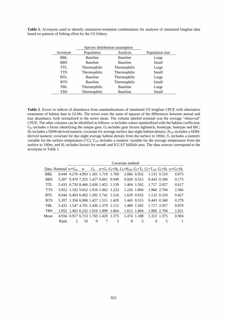
Table 1. Acronyms used to identify simulation-treatment combinations for analyses of simulated longline data
based on patterns of fishing effort by the US fishery.
Species distribution assumption Acronym Population Analysis Population size
BBL Baseline Baseline Large
BBS Baseline Baseline Small
TTL Thermophilic Thermophilic Large
TTS Thermophilic Thermophilic Small
BTL Baseline Thermophilic Large
BTS Baseline Thermophilic Small
TBL Thermophilic Baseline Large
TBS Thermophilic Baseline Small
Table 2. Errors in indices of abundance from standardizations of simulated US longline CPUE with alternative
treatments of habitat data in GLMs. The errors were the sums of squares of the differences between annual and
true abundance, both normalized to the series mean. The column labeled nominal was the average “observed”
CPUE. The other columns can be identified as follows: w includes values standardized with the habitat coefficient;
Gid includes a factor identifying the unique gear; Gf includes gear factors lightstick, hooktype, baittype and hbf ;
H0 includes a SDM-derived numeric covariate for average surface day-night habitat density; H100 includes a SDM-
derived numeric covariate for day-night average habitat density from the surface to 100m; T0 includes a numeric
variable for the surface temperature (°C); T100 includes a numeric variable for the average temperature from the
surface to 100m; and Hf includes factors for month and ICCAT billfish area. The data sources correspond to the
acronyms in Table 1.
Covariate method
Data Nominal w+Gid w Gf w+Gf Gf+H0 Gf+H100 Gf+T0 Gf+T100 Gf+Hf w+Gf+Hf
BBL 6.044 0.276 4.993 1.281 1.719 1.769 2.066 0.932 1.133 0.310 0.875
BBS 5.207 0.470 7.255 1.427 0.601 0.949 0.920 0.515 0.443 0.340 0.175
TTL 5.433 0.720 8.466 2.436 1.452 1.139 1.404 1.502 1.717 2.057 0.617
TTS 3.052 1.102 9.652 1.916 1.062 1.233 1.226 1.804 1.960 2.794 2.366
BTL 6.044 0.403 6.402 1.281 1.741 1.516 1.629 0.932 1.133 0.310 0.427
BTS 5.207 1.356 6.006 1.427 1.511 1.420 1.445 0.515 0.443 0.340 0.279
TBL 5.433 1.547 4.701 2.436 1.379 1.112 1.489 1.502 1.717 2.057 0.870
TBS 3.052 1.465 6.232 1.916 1.899 1.864 1.613 1.804 1.960 2.794 1.621
Mean 4.934 0.917 6.713 1.765 1.420 1.375 1.474 1.188 1.313 1.375 0.904
Rank 2 10 9 7 5 8 3 4 5 1
926
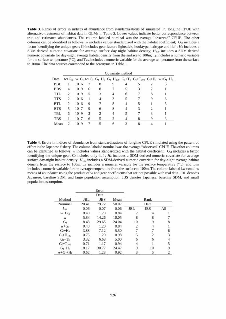
Table 3. Ranks of errors in indices of abundance from standardizations of simulated US longline CPUE with
alternative treatments of habitat data in GLMs in Table 2. Lower values indicate better correspondence between
true and estimated abundances. The column labeled nominal was the average “observed” CPUE. The other
columns can be identified as follows: w includes values standardized with the habitat coefficient; Gid includes a
factor identifying the unique gear; Gf includes gear factors lightstick, hooktype, baittype and hbf ; H0 includes a
SDM-derived numeric covariate for average surface day-night habitat density; H100 includes a SDM-derived
numeric covariate for day-night average habitat density from the surface to 100m; T0 includes a numeric variable
for the surface temperature (°C); and T100 includes a numeric variable for the average temperature from the surface
to 100m. The data sources correspond to the acronyms in Table 1.
Table 4. Errors in indices of abundance from standardizations of longline CPUE simulated using the pattern of
effort in the Japanese fishery. The column labeled nominal was the average “observed” CPUE. The other columns
can be identified as follows: w includes values standardized with the habitat coefficient; Gid includes a factor
identifying the unique gear; Gf includes only hbf ; H0 includes a SDM-derived numeric covariate for average
surface day-night habitat density; H100 includes a SDM-derived numeric covariate for day-night average habitat
density from the surface to 100m; T0 includes a numeric variable for the surface temperature (°C); and T100
includes a numeric variable for the average temperature from the surface to 100m. The column labeled kw contains
means of abundance using the product of w and gear coefficients that are not possible with real data. JBL denotes
Japanese, baseline SDM, and large population assumption. JBS denotes Japanese, baseline SDM, and small
population assumption.
Error
Data Method JBL JBS Mean Rank
Nominal 20.41 79.72 50.07 Data
kw 0.06 0.07 0.06 JBL JBS All
w+Gid 0.48 1.20 0.84 2 4 1
w 5.83 14.26 10.05 8 8 7
Gf 18.43 29.65 24.04 10 9 8
w+Gf 0.48 1.20 0.84 2 4 1
Gf+H0 3.88 7.12 5.50 7 7 6
Gf+H100 0.75 1.20 0.98 5 2 3
Gf+T0 3.32 6.68 5.00 6 6 4
Gf+T100 0.71 1.17 0.94 4 1 5
Gf+Hf 18.17 30.77 24.47 9 10 9
w+Gf+Hf 0.62 1.23 0.92 3 5 2
Covariate method
Data w+Gid w Gf w+Gf Gf+H0 Gf+H100 Gf+T0 Gf+T100 Gf+Hf w+Gf+Hf
BBL 1 10 6 7 8 9 4 5 2 3
BBS 4 10 9 6 8 7 5 3 2 1
TTL 2 10 9 5 3 4 6 7 8 1
TTS 2 10 6 1 4 3 5 7 9 8
BTL 2 10 6 9 7 8 4 5 1 3
BTS 5 10 7 9 6 8 4 3 2 1
TBL 6 10 9 3 2 4 5 7 8 1
TBS 1 10 7 6 5 2 4 8 9 3
Mean 2 10 9 7 5 6 3 8 4 1
927
Figure 1. Observed and simulated catches for the population trend used in the simulations.
Figure 2. Population trajectories used in the longline data simulations.
928
Figure 3. Temperature suitability curves for the alternative species distribution models used in this analysis.
Figure 4. Content of data records used as input for analysis using a GLM and source of data for each field. The
catch, effort (number of hooks), month, year and location are extracted from a source of catch and effort
information. Matching gear related data (gear-g4 and hbf [hooks between floats]) are included from a source of
gear information. Temperature at the surface (T0, the SST) and the average temperature from the surface to 100m
(T100) are obtained from a source of environmental data. The value of the habitat at the surface, H0, and from the
surface to 100m (H100) are computed using a Species Distribution Model (SDM) using important habitat variables.
The habitat coefficient, w, is computed from gear characteristics and environmental data using the SDM for the
time and place specified for the catch in the CPUE file.
929
Figure 5. Deterministic estimates of population size from the longline catches simulated using the distribution of
Japanese fishing effort and assuming the baseline SDM and small population scenario. The data were summarized
at 1° or 5° spatial resolution for the region 50S to 50N (trim) or 50S to 55N (Full).
930
Figure 6. True population trend and abundance indices from various treatments of simulated US longline catches
for blue marlin. The simulations assumed the large population option and the baseline distribution pattern.
Analyses assumed the baseline distribution. The nominal and determinist estimates are in panel A. Other panels
apply various combinations of factors and numerical variables in GLM-based standardizations as indicated.
931
Figure 7. True population trend and abundance indices from various treatments of simulated US longline catches
for blue marlin. The simulations assumed the small population option and the baseline distribution pattern.
Analyses assumed the baseline distribution. The nominal and determinist estimates are in panel A. Other panels
apply various combinations of factors and numerical variables in GLM-based standardizations as indicated.
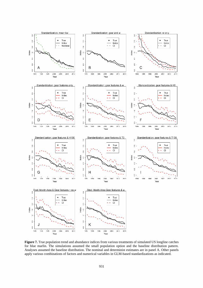
932
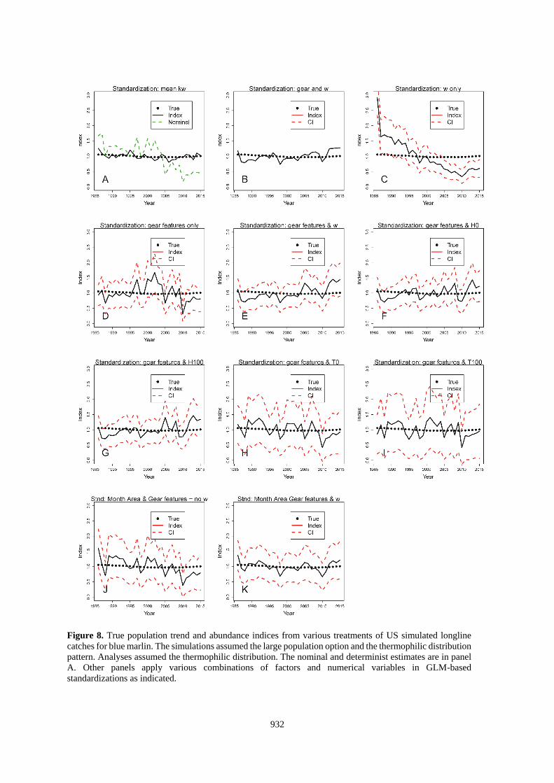
Figure 8. True population trend and abundance indices from various treatments of US simulated longline
catches for blue marlin. The simulations assumed the large population option and the thermophilic distribution
pattern. Analyses assumed the thermophilic distribution. The nominal and determinist estimates are in panel
A. Other panels apply various combinations of factors and numerical variables in GLM-based
standardizations as indicated.
933
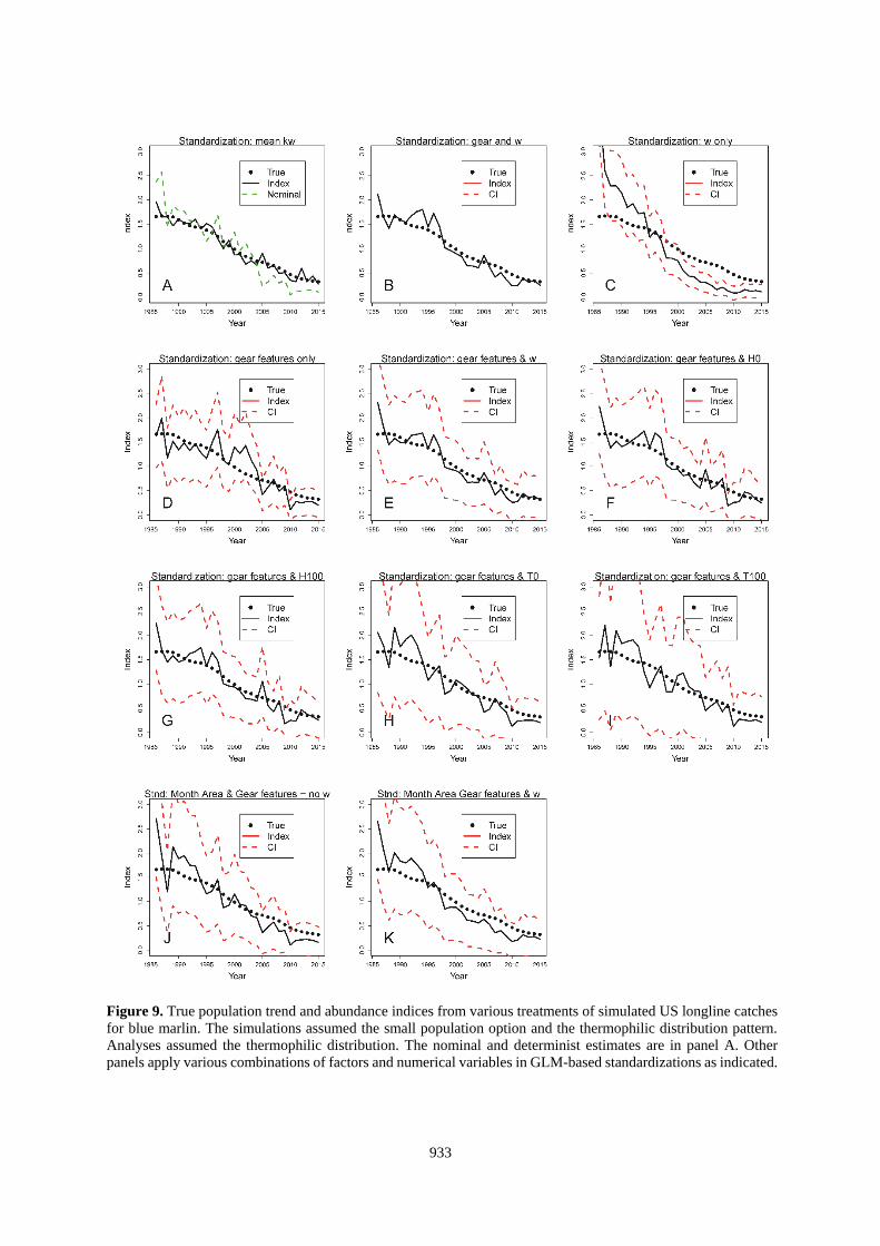
Figure 9. True population trend and abundance indices from various treatments of simulated US longline catches
for blue marlin. The simulations assumed the small population option and the thermophilic distribution pattern.
Analyses assumed the thermophilic distribution. The nominal and determinist estimates are in panel A. Other
panels apply various combinations of factors and numerical variables in GLM-based standardizations as indicated.
934
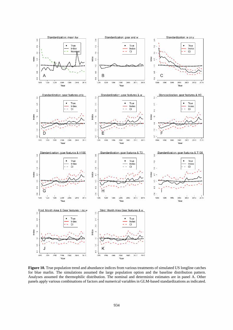
Figure 10. True population trend and abundance indices from various treatments of simulated US longline catches
for blue marlin. The simulations assumed the large population option and the baseline distribution pattern.
Analyses assumed the thermophilic distribution. The nominal and determinist estimates are in panel A. Other
panels apply various combinations of factors and numerical variables in GLM-based standardizations as indicated.
935
Figure 11. True population trend and abundance indices from various treatments of simulated US longline catches
for blue marlin. The simulations assumed the small population option and the baseline distribution pattern.
Analyses assumed the thermophilic distribution. The nominal and determinist estimates are in panel A. Other
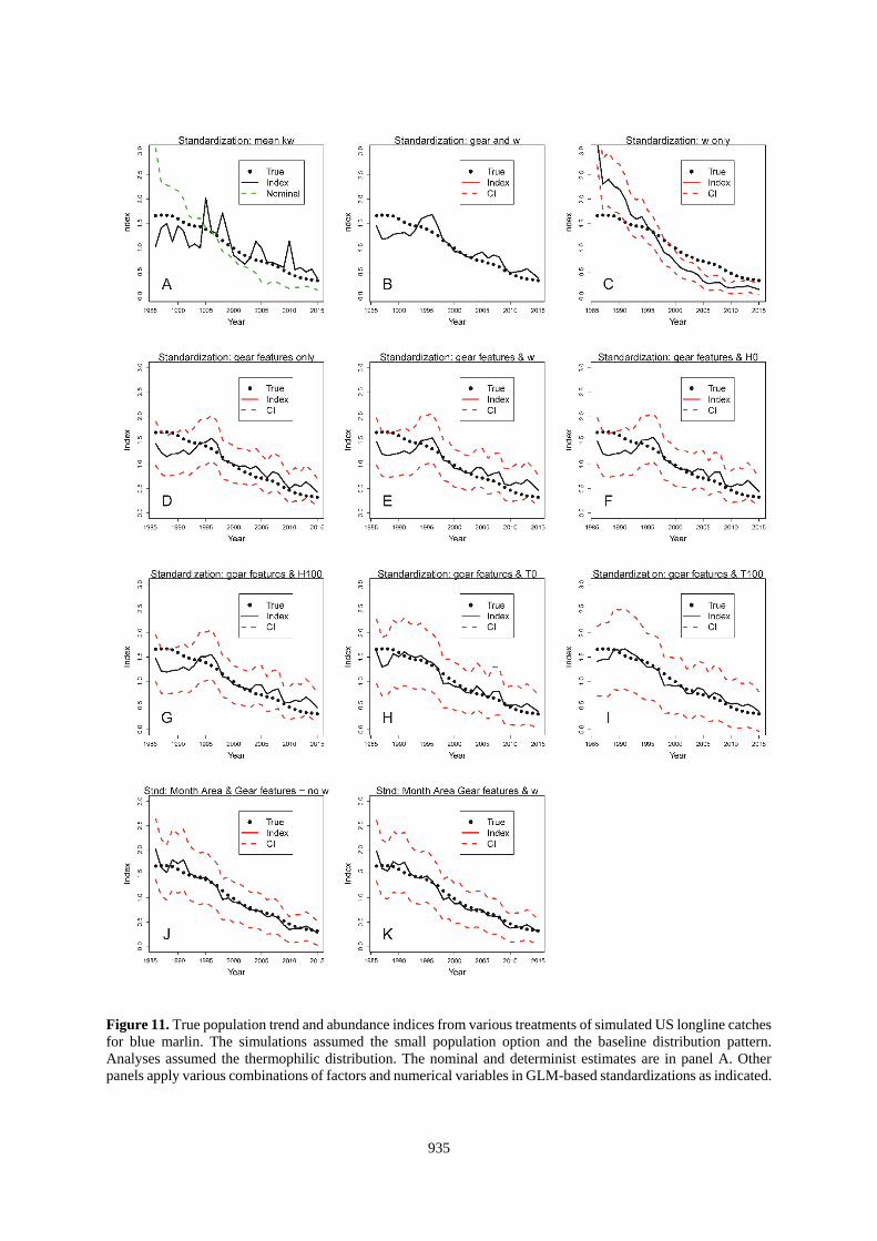
panels apply various combinations of factors and numerical variables in GLM-based standardizations as indicated.
936
Figure 12. True population trend and abundance indices from various treatments of simulated US longline catches
for blue marlin. The simulations assumed the large population option and the thermophilic distribution pattern.
Analyses assumed the baseline distribution. The nominal and determinist estimates are in panel A. Other panels
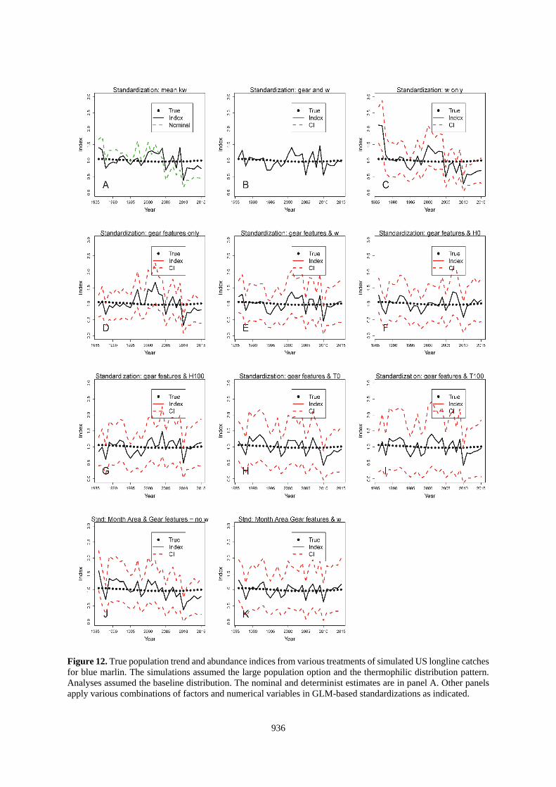
apply various combinations of factors and numerical variables in GLM-based standardizations as indicated.
937
Figure 13. True population trend and abundance indices from various treatments of simulated US longline catches
for blue marlin. The simulations assumed the small population option and the thermophilic distribution pattern.
Analyses assumed the baseline distribution. The nominal and determinist estimates are in panel A. Other panels
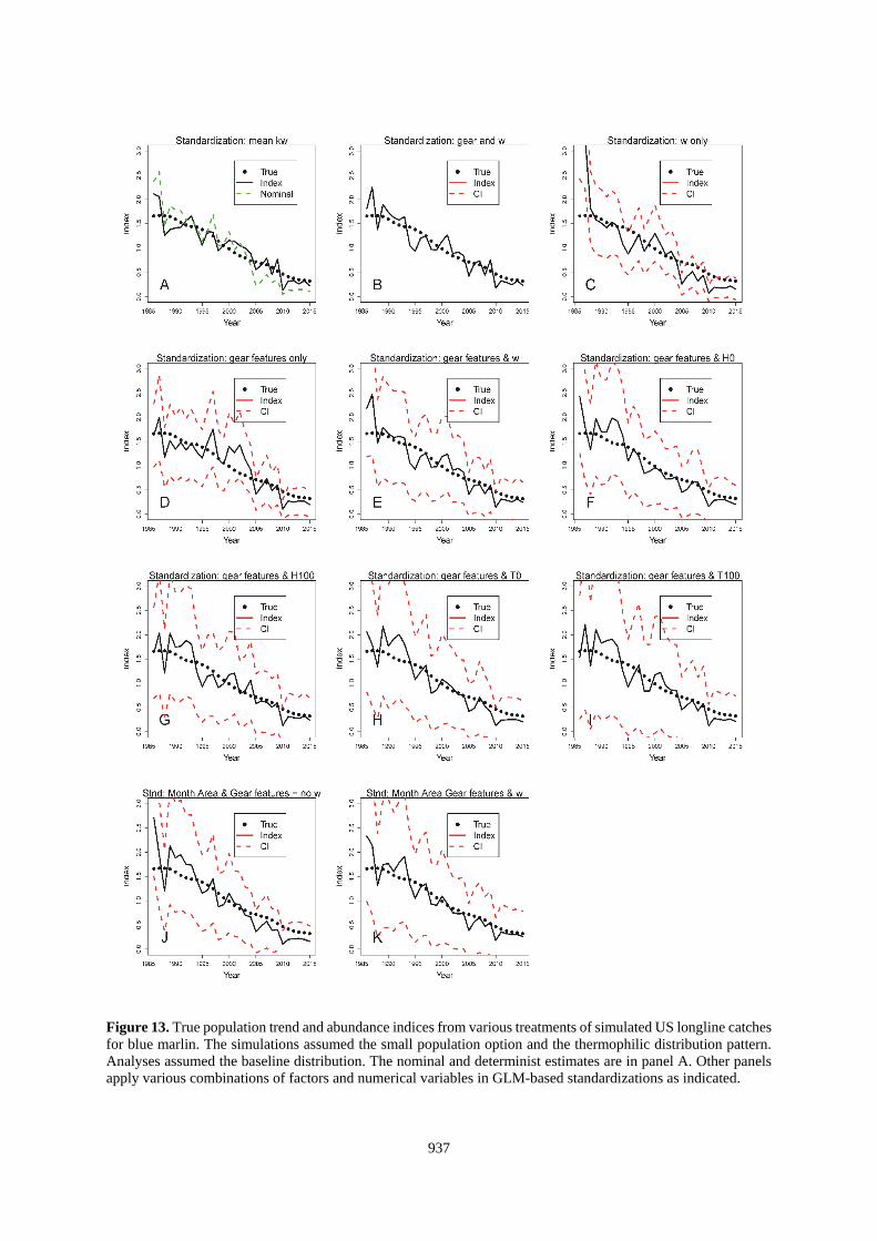
apply various combinations of factors and numerical variables in GLM-based standardizations as indicated.
938
Figure 14. True population trend and abundance indices from various treatments of longline catches for blue
marlin simulated with fishing patterns similar to the Japanese fishery. The simulations assumed the large
population option and the baseline distribution pattern. Analyses assumed the baseline distribution. The nominal
and determinist estimates are in panel A. Other panels apply various combinations of factors and numerical
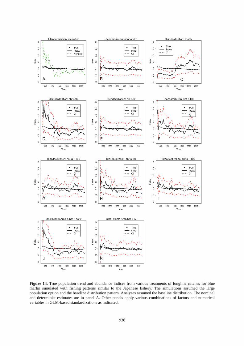
variables in GLM-based standardizations as indicated.
939
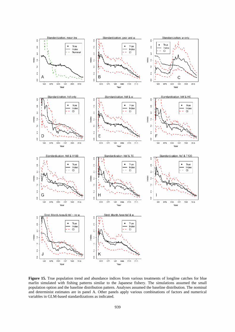
Figure 15. True population trend and abundance indices from various treatments of longline catches for blue
marlin simulated with fishing patterns similar to the Japanese fishery. The simulations assumed the small
population option and the baseline distribution pattern. Analyses assumed the baseline distribution. The nominal
and determinist estimates are in panel A. Other panels apply various combinations of factors and numerical
variables in GLM-based standardizations as indicated.