Habit Formation and Naivet e in Gym Attendance: …...Habit Formation and Naivet e in Gym...

Habit Formation and Naivete in Gym Attendance:Evidence from a Field Experiment∗

Dan AclandUC Berkeley

[email protected]

Matthew LevyHarvard University

[email protected]

February 16, 2010

Abstract

We extend the gym-attendance study of Charness and Gneezy (2009) byincentivizing subjects to attend the gym for a month, observing their pre- andpost-treatment attendance relative to a control group, and eliciting subjects’pre- and post-treatment predictions of their post-treatment attendance. Wefind a habit formation effect similar to that of Charness and Gneezy in the short-run, but with substantial decay caused by winter vacation. We additionally findthat subjects seriously over-predict future attendance, which we interpret asevidence of partial naivete with respect to self-control problems. Subjects alsoappear to have biased beliefs about their future cost of gym attendance. Ourdesign allows us to estimate the monetary value of habit formation—equivalenton average to a $0.40 per visit subsidy—as well as the welfare cost of presentbias and naivete.

Keywords: Exercise, Field experiment, Habit formation, Quasi-hyperbolic dis-counting

∗Financial support was provided by the National Institute on Aging through the Center on theEconomics and Demography of Aging at UC Berkeley, grant number P30 AG12839. The authorswould like to thank Stefano DellaVigna, Gary Charness, Uri Gneezy, Teck Hua Ho, Shachar Kariv,Botond Koszegi, Ulrike Malmendier, Alexander Mas, Matthew Rabin, and all of the participantsin the UC Berkeley Psychology and Economics Non-Lunch for helpful comments. Special thanksgo to Brenda Naputi of the Social Science Experimental Laboratory at the Haas School of Busi-ness, Brigitte Lossing at the UC Berkeley Recreational Sports Facility, and to Vinci Chow andMichael Urbancic of the UC Berkeley Department of Economics, for extraordinary assistance withimplementation.

1

mailto:[email protected]

mailto:[email protected]

1 Introduction

Incentivizing healthy behaviors, and in particular physical exercise, has received in-

creasing interest in various literatures in the face of growing concern about the cost

of health care and the increasing problem of obesity. Of particular interest is the po-

tential to build long-term healthy behaviors with short-term incentive interventions.1

Charness and Gneezy (2009) provided the first experimental evidence on this possibil-

ity in the domain of physical exercise, showing that paying a group of undergraduates

to attend the gym for a month raises attendance in the subsequent weeks, despite the

removal of the incentive. This effect can be interpreted as habit formation.

Their study raises a number of interesting questions that deserve further investi-

gation. How does the habit decay over time? What is the role of self-control problems

in gym attendance? How well do subjects predict various dimensions of their future

gym attendance? And is it possible to calibrate the value of the habit? These are key

to understanding the welfare effects of the intervention, as well as its policy relevance.

In this paper, we present evidence from a field experiment designed to answer these

questions.

Charness and Gneezy paid undergraduates to attend the gym for four weeks and

found that, after the payment ended, treated subjects had significantly higher gym

attendance than did a control group. Their subjects were university undergraduates

who were randomized into three groups.2 A “low incentive” group were offered $25 to

attend the gym once during the initial week of the study. A “high incentive” group

received the same $25 offer, and were additionally offered $100 to attend the gym

another eight times in the subsequent four weeks for a total of nine visits over five

weeks. A control group received no offers for gym attendance. Gym-attendance data

was collected for all subjects for a period beginning eight weeks before the treatment

and ending seven weeks after. By comparing the pre- to post-treatment change in

attendance across groups they are able to show that subjects in the high-incentive

group continue to have significantly higher gym attendance after the incentive period

ends than subjects in the other two groups—an average of 0.67 visits per week more

than the control group, and 0.58 visits per week more than the low-incentive group.

1See Kane, Johnson, Town and Butler (2004) for a review.2We are describing Charness and Gneezy’s first study, which our experiment is most similar to.

In the same paper they conducted a second study with a slightly different design that yielded similarresults.

2

Furthermore, they found that the increase came from the subset of subjects who

had previously attended less than once per week on average, which they refer to as

non-regular attenders.

To explore our questions of interest we built on Charness and Gneezy’s high-

incentive and low-incentive treatments. We recruited 120 subjects who were self-

reported non-regular gym attenders. We then collected gym attendance data covering

a span of seventeen months, allowing us to investigate habit decay more thoroughly.

Further, in addition to the $25 and $100 attendance incentives, we used an incentive-

compatible mechanism to elicit subjects’ predictions of their post-treatment gym-

attendance, conducting the elicitation both immediately before and immediately after

the treatment period, allowing us to explore issues of mis-prediction. Finally, the

elicitation mechanism involved offering small attendance incentives in some of the

post-treatment weeks, which allows us to estimate the costs and benefits associated

with the habit.

We find a short-run habit-formation effect among our subjects of 0.256 visits

per week, which is smaller than, but statistically indistinguishable from, Charness

and Gneezy’s result. However, the effect appears to largely decay over the course

of winter vacation. Moreover, this treatment effect is highly concentrated in the

upper tail of the post-treatment attendance distribution. We also find that subjects

substantially over-predict their future gym attendance: even in our simplest elicitation

task, subjects over-predicted attendance by roughly a factor of three. Predictions are

closer to actual attendance after the treatment period than before. By fixing the

delay between the week in which predictions are made and the week about which

they are made, we rule out intertemporal discounting as an explanation for this shift,

suggesting that subjects also mispredict some other aspect of their gym-attendance

decision, such as the opportunity cost of attendance. Finally, we estimate two key

parameters of the model: the dollar value of the habit-formation effect, and the value

of the unforeseen portion of the foregone long-term gym-attendance benefit lost due to

self-control problems. We find that the habit induced in treated subjects is equivalent

on average to a $0.40 per visit subsidy, or $4.50 per visit among subjects we identify

as habit-formers. The cost of naivete is also large, and indicates that the intervention

may be welfare-enhancing.3 Using these parameters, we set forty-six weeks as an

3By contrast, in a model without time-inconsistency this intervention would increase long-rungym attendance but be inefficient relative to a lump-sum transfer to subjects.

3

upper bound on how long habituated subjects must retain their gym habit for the

intervention to be cost-effective.

The paper unfolds as follows. Section two presents our model and our parameter-

estimation strategy. Section three describes our experimental design. Results are

presented in section four. Section five concludes.

2 Model

In this section we develop a simple model of gym attendance that incorporates habit

formation and present-biased preferences. Habit—caused by past gym attendance—

is modeled as a fixed, additive increase in gym-attendance utility, a la Becker and

Murphy (1988) and O’Donoghue and Rabin (1999a). Individuals discount all future

periods relative to the present, a la Phelps and Pollak (1968) and Laibson (1997),

and are naive or sophisticated with respect to this “quasi-hyperbollic discounting”, a

la O’Donoghue and Rabin (1999b).

In the spirit of DellaVigna and Malmendier (2004), we consider a finite-horizon,

discrete-time model with five unequal periods. Initially all subjects are non-habituated,

and are randomly divided into two groups, one of which will be incentivized to attend

the gym in period one (treated group), and the other of which will not (control group).

In the first period subjects bid, in an incentive compatible auction, on a “p-coupon”,

a certificate that rewards fourth-period gym attendance, and then predict how many

times they will go to the gym that period if they win the coupon.4 Then, still in the

first period, treated subjects attend the gym and develop a habit that will persist

through all subsequent periods.

In the second period two things happen. First subjects once again bid on the

fourth-period p-coupon and predict their fourth-period attendance. Then, after the

auction, all subjects are given a p-coupon.5 Period three acts as a buffer, ensuring

that subjects consider the target period to be “in the future” when predictions are

elicited. In period four, subjects receive p-coupon rewards according to their gym

attendance in that period. We explicitly think of periods three and four as weeks,

4We refer to period four as the “target-week” as it is the target of the p-coupon.5In the model we are ignoring the fact that the elicitation process requires one or two subjects

to wind up with two coupons. In practice, because there were multiple target weeks, most of theauction winners did not end up holding multiple p-coupons for the same week. The two subjectswho did wind up with two p-coupons for the same target week simply received double the reward.

4

during which subjects decide each day whether to attend the gym that day. Finally,

in period five subjects receive the delayed health benefit of whatever gym attendance

they have engaged in.

Let the immediate utility of gym attendance on day d be −c + εd with c > 0,

and i.i.d. εd ∼ F. Let the delayed benefit of gym attendance be b > 0. Thus we

model gym attendance as an “investment good” in the language of DellaVigna and

Malmendier, meaning that costs are immediate while rewards are delayed. Future

payoffs are discounted by β, with beliefs about future self-control denoted by β.6

Following O’Donoghue and Rabin (1999a), habit formation takes a simple binary

form. When subjects are habituated they receive additional, immediate utility for

gym attendance of η > 0, so that the immediate utility of gym attendance for a

habituated subject is η − c + εd. We model utility as quasi-linear in money. Utility

from all non-gym sources is normalized to zero.

Let P be the face value of the p-coupon that rewards gym attendance in period

four. That is, a p-coupon pays $P , immediately, for each day that the holder attends

the gym in period four. Let Xgt refer to the valuation of a p-coupon in period t = 1, 2

of a subject in group g = 0, 1 (control=0, treated=1). Let Zg be the number of days

of gym attendance during the target week for a subject in group g.

2.1 Attendance decision and the value of a p-coupon.

If a subject attends the gym on a given day during the target week her utility for

that day will be P +βb+gη− c+εd. She will attend the gym if this is positive. Thus

Zg =7∑d=1

1 · {εd > P +βb+gη− c}. In expectation, total target-week gym-attendance

will be,

7∑d=1

Pr(εd > P + βb+ gη − c) = 7×∞∫

c−βb−gη−P

dF (ε). (1)

However, from the perspective of any previous period, the perceived probability

of target-week gym-attendance depends upon the subject’s belief about future self-

control, β. She believes she will attend on any given day of the target week if εd >

P + βb + gη − c. Thus the subject’s ex-ante prediction of her total utility for the

6Because of the short time horizon, we assume no long-run discounting, i.e. δ = 1.

5

target-week, given that she holds a p-coupon, is,

7×∞∫

c−bβb−gη−P(P + b+ gη − c+ ε) dF (ε). (2)

Setting P to zero gives us the predicted utility without a p-coupon. The value of the

p-coupon, from the perspective of either period one or period two, is the difference

between expected utility with a p-coupon and expected utility without a p-coupon,

which is,

Xg1 = Xg

2 =

7×∞∫

c−bβb−gη−PP dF (ε)

+

7×c−bβb−gη∫

c−bβb−gη−P(b+ gη − c+ ε) dF (ε)

. (3)

Note that this valuation is the same for pre- and post-treatment elicitations be-

cause the target week is in the future (hence “inside β”) from the perspective of either

elicitation period. The first term in the expression is the expected redemption value

of the coupon, which is always weakly positive. The second term is the subject’s val-

uation of the behavioral change that results from holding the coupon, which we will

call the incentive value. This is the change in utility caused by those gym-visits that

the subject would not have made in the absence of the p-coupon. The sign depends on

the subject’s ex-ante belief about future self-control problems. If the subject believes

that she will not have self-control problems in the target week, the incentive value is

negative because the subject believes that the p-coupon will make her attend the gym

when the direct utility of doing so is negative. If the subject believes that she will

have self-control problems in the target week, then the incentive value may be positive

because she may foresee that the p-coupon will make her more likely to attend the

gym and gain a long-term benefit that she would otherwise forego due to self-control

problems.7 Note that the net value of the p-coupon is always non-negative.

7Thus, for a sophisticate with self-control problems the incentive value can be thought of as“commitment value” because it is the value of having the p-coupon as a “commitment device” tohelp her get out the door and down to the gym.

6

2.2 Parameter Identification

We focus our analysis on two parameters that are key to evaluating the welfare effects

of the intervention and which can be estimated in a parsimonious two-equation sys-

tem. The first is the habit-formation effect itself, η, which is the additional, per-visit,

gym-attendance utility (measured in dollars) received by a subject in the habituated

state. Another way to think of this parameter is that η is the per-visit monetary

incentive that would cause a non-habituated subject to attend as often as an unin-

centivized habituted subject. The second term we are interested in estimating is the

per-visit cost of naivete with respect to self-control, (β−β)b. This is the dollar value

of the portion of the per-visit future benefit of gym attendance, b, that present bias

makes a subject willing to forego, but which a naif fails to foresee.

The first parameter of interest is η, the habit value. Our estimation strategy is

essentially equivalent to finding the value of P for which the average target-week

attendance in the control group, with a p-coupon, is the same as the average target-

week attendance in the treated group, without a p-coupon. Let Zg

p be the average

weekly attendance of subjects in group g ∈ {T,C} who are holding a p-coupon, and

Zg

0 be the same thing for subjects with no p-coupon (i.e. P = 0). In terms of our

model, we are looking for P ∗ such that,

ZT

0 = 7×∞∫

c−βb− η

dF (ε) = 7×∞∫

c−βb−P ∗

dF (ε) = ZC

p . (4)

Once we know the value of P ∗, because F (·) is monotonically increasing, we then

have η = P ∗.

The cost of naivete, (β − β)b, is identified by comparing the control group’s pre-

dicted target-week attendance with their actual attendance. Let Yg

p be the average,

unincentivized prediction, in either elicitation session, of gym attendance during a

target week with a p-coupon of subjects in group g. The average unincentivized pre-

diction of gym attendance in a target week with a p-coupon with a face value of P ,

among control subjects, is

YC

p = 7×∞∫

c−bβb− ePdF (ε) = 7×

∞∫c−βb−(bβb−βb)− eP

dF (ε). (5)

7

We find the value of P ∗ for which

YC

p = 7×∞∫

c−βb−(bβb−βb)− ePdF (ε) = 7×

∞∫c−βb−P ∗

dF (ε) = ZC

p , (6)

which gives us (β − β)b = P ∗ − P . In practice we will evaluate this by setting P

equal to the average value of P among all control subjects. We estimate the moment

equations in (4) and (6) in section 4.3.

3 Design

We recruited one hundred and twenty subjects from the students and staff of UC

Berkeley and randomly assigned them to treated and control groups.8 Since Charness

and Gneezy found the habit-formation effect concentrated among non-attenders we

screened for subjects who self-reported that they had not ever regularly attended any

fitness facility.9 Treated and control subjects met in separate sessions on the same day,

at the beginning of the second week of the fall semester of 2008. Both treatment and

control subjects were asked to complete a questionnaire, and were then given an offer

of $25 to attend the gym once during the following week.10 We call this the “learning

week” offer, and it is identical to Charness and Gneezy’s low-incentive condition. Our

control group is therefore comparable to Charness and Gneezy’s low-incentive group.

We chose this as our control in order to separate the effect of overcoming the one-time

fixed cost of learning about the gym from the actual habit formation that occurs after

multiple visits.11

At the same initial meeting, the treatment group received an additional offer of

$100 to attend the gym twice a week in each of the four weeks following the learning

week. We call this the treatment-month offer, and it is the same as Charness and

Gneezy’s high-incentive offer, except that they did not require the eight visits to be

8Due to attrition and missing covariates, our final sample includes 54 treated subjects and 57control subjects. Details of the sample appear in appendix A.1.

9Our screening mechanism is described in appendix A.2.10For this and all subsequent offers, subjects were told that a visit needed to involve at least 30

minutes of some kind of physical activity at the gym. We were not able to observe actual behaviorat the gym and did not claim that we would be monitoring activity.

11We also paid the $10 gym-membership fee for all students, and filed the necessary membershipforms for those who were not already members.

8

Dead Week(1 week, both groups)

Announce both offers:L-W ($25 for 1 visit)

T-M ($100 for 2 visits/wk, 8 total, Treated group only)

Pre-treatment Predictions

Treatment Month (T-M)

(4 weeks, Treatedgroup only)

Pre-treatment Period(37 weeks, both groups)

Learning Week (L-W)(1 week, both groups)

Post-treatmentPeriod

(33 weeks,both groups)

Target Weeks(5 weeks, both groups)

Post-treatment Predictions

Treatment Control

Remaining Post-treatment Period (33-6=27 weeks, both groups)

Figure 1: Our Experimental Design

evenly spaced across the four weeks. The other difference between this offer and

Charness and Gneezy’s high-incentive offer is that we made our offer at the first

meeting, at the same time as the $25 learning-week offer, whereas Charness and

Gneezy made their high-incentive offer at their second meeting, a week later. We

made our treatment-month offer earlier because we wanted Treated subjects to have

a week to contemplate the idea of going to the gym twice weekly for a month before

making predictions. Moreover, if subjects have reference-dependent preferences for

money then suddenly announcing a gain of $100 to one group but not the other could

introduce systematic bias into the incentive compatible procedure we used to elicit

predictions. Waiting a week after treatment subjects learn they will earn $100 will

help us overcome a potential “house money effect”.

At the end of the learning week both groups of subjects again met separately and

completed pencil-and-paper tasks (described in detail below) designed to elicit their

predictions of gym attendance during each of five post-treatment “target weeks”.

Both groups were reminded of the offers they had received. Four weeks later, at

the end of the treatment month, both groups again met separately, completed an

9

additional questionnaire, and completed the same elicitation tasks as in the second

session. The target weeks were separated from this second elicitation session by a

dead week so that present-biased subjects would see the target weeks as being “in

the future” from the perspective of both elicitation sessions. The timeline of the

experiment is illustrated in Figure 1.

Gym attendance data were collected for a 17-month period stretching from 37

weeks before the learning week to 33 weeks after it. This period includes summer and

winter breaks as well as three full semesters.

3.1 Elicitation procedures

To elicit predictions of target-week gym attendance we created what we call a “p-

coupon”, which is a certificate that rewards the holder with $P for each day that he or

she attends the gym during a specified “target week”. The value of P , which ranged

from $1 to $7, was printed on the coupon, along with the beginning and end dates

of the target-week. We used an incentive-compatible mechanism to elicit subjects’

valuations for p-coupons of various values with various target weeks.12 Subjects’

incentive-compatible bids for a p-coupon are correlated with how many times they

think they will attend the gym during the target week of the coupon. A sample

p-coupon is included in appendix A.3, along with the pencil-and-paper task we used

to elicit valuations for p-coupons, the instructions we gave them for completing the

task, and further description of how the elicitation mechanism worked. Each subject

completed this incentive-compatible elicitation task for four of the five target weeks

in our design, and for a different value of p-coupon in each of those four weeks. The

values of the p-coupons for the different weeks was randomized among subjects, as

was the order in which those weeks were presented.13

Subjects’ bids for a coupon that pays out as a function of the number of times

a certain event occurs in a future target week need not be based entirely on their

predictions of how many times that event will occur. Risk-aversion implies we would

12Subjects made a series of choices between a p-coupon and an incrementally increasing fixedamount of money. We infer their valuation from the indifference point between the coupon and thefixed sum. The elicitation mechanism is described in detail in appendix A.3.

13Thus subjects did not all bid on a p-coupon for target-week one, then target-week two, etc, nordid all subjects bid on p-coupons of the same size for each of the target weeks. Among each subject-group/target-week intersection, subgroups of fifteen subjects received $1, $2, and $3 coupons, tenreceived $5 coupons, and five received $7 coupons.

10

only observe subjects’ certainty equivalents, even for an exogenous event.14 But

for an endogenous event like gym attendance, there is the additional confound that

the p-coupon itself incentivizes the subject to go to the gym, thus influencing the

very behavior we are asking them to predict. This “incentive effect” may increase

or decrease subjects’ bids for a p-coupon, and care must therefore be taken not to

interpret subjects’ bids as directly proportional to their beliefs.

As a check on this mechanism, we also directly asked subjects to state how many

times they thought they would go to the gym during the specified target weeks if they

had been given the p-coupon they just bid on in the incentive-compatible task. Thus

they were making unincentivized predictions of hypothetical future attendance under

the same set of attendance incentives as in the incentivized task.15 This unincentivized

mechanism also allowed us to ask subjects how often they thought they would go to

the gym during the one target week for which they were not presented with a p-

coupon, the so-called “zero week” (because it is equivalent to a P of zero). The zero

week gives us an additional unincentivized prediction of behavior in the absence of

any effect of attendance incentives.

Subjects went through exactly the same set of elicitation tasks in both the pre-

treatment and post-treatment elicitation sessions. Then, at the end of the second

elicitation session, after all of the elicitation tasks had been completed, each subject

was given one of the four coupons they had been presented with during the elicitation

process. These give-away coupons were in addition to those that had been won earlier

in the bidding process. We therefore have two target weeks for each subject in which

we can compare their predictions with their actual gym attendance under the same

conditions, the first being the zero-week, and the second being the week for which they

received a p-coupon in the giveaway. The giveaway was a surprise to the subjects—

having been conducted unannounced only after the second elicitation session—and

thus did not affect their bids or unincentivized responses during the elicitation tasks.

We discuss compliance with the treatment incentive, attrition, and our random-

ization procedure in appendix A.4.

14An alternative design which would have allowed us to sidestep assumptions about the linearityof money utility, would have been to have the coupons pay off not with a dollar sum per visit, butwith a per-visit increment in the cumulative probability of winning some fixed-sum prize. We believeour design is more intuitive for subjects, and easier for them to understand.

15It is important to note that the p-coupons incentivize both target-week attendance and accuratepredictions of target-week attendance.

11

4 Results

Of the 54 subjects in our final treatment sample, 43 completed the eight necessary

bi-weekly visits in order to earn the $100 incentive: a compliance rate of 80%. In

Charness and Gneezy’s (2009) high-incentive group the compliance rate was approx-

imately 83%, suggesting that our more restrictive design did not have a significant

effect on subjects’ ability to make the required number of visits. It is notable that

our sample of non gym-attenders were so easily induced to visit the gym eight times.

4.1 Habit formation

Figure 2 shows average weekly attendance for the treated and control groups over

the duration of the study period.16 In the pre-treatment period, attendance in the

two groups moves together tightly. In the treatment period, treated subjects attend

much more than control subjects. In the two months immediately following the

treatment period, leading up to, but not including winter vacation, the treatment

group consistently attends the gym more than the control group. In the four months

after the winter vacation the graph suggests persistence of the increased treatement-

group attendance, but the difference is not as striking.

We estimate a linear, difference-in-differences, panel regression model to see if

these patterns are statistically significant. Each observation in the panel is a specific

individual on a specific week of the study.17 We regress weekly gym attendance on

a treated-group dummy, a set of week-of-study dummies, and the interactions of the

treated-group dummy with dummies for the treatment period and each of the two

post-treatment periods. The results of this regression appear in the first column of

Table 1.

The coefficient on the treated-group dummy tells us that there is no statistically

significant difference in gym attendance between treated and control subjects in the

pre-treatment period. The coefficient on the interaction of the treated-group and

treatment-period dummies, roughly the product of the twice-weekly incentive target

and the 80% compliance rate, reassures us that the treatment-incentive was effective.

The remaining two interaction terms tell us the effect of the treatment on treated-

16We have removed observations for target weeks when subjects received p-coupons to make thegraph easier to read.

17We again exclude observations for the one target week for each subject for which they receivedan actual p-coupon.

12

Table 1: Habit Formation: Regression of average weekly attendance.

(1) (2) (3)(Charness&Gneezy)

Treated 0.045 0.045 -0.100(0.057) (0.057) (0.196)

[0.477]a

Treatment Period X Treated 1.321∗∗∗ 1.209∗∗∗ 1.275∗∗∗

(0.134) (0.150) (0.181)[0.780]a

Imm. Post-Trmt X Treatedb 0.129 0.256∗∗ 0.585∗∗∗

(0.111) (0.122) (0.217)[0.186]a

Later Post-Trmt x Treatedb 0.050 0.045 –(0.095) (0.098)

Complied w/ treatment 0.057(0.071)

Treatment Period X Complied 1.582∗∗∗

(0.180)Imm. Post-Trmt X Complianceb 0.338∗∗

(0.154)Later Post-Trmt x Complianceb 0.061

(0.126)

Week Efffects Yes Yes Yes YesControls – Yes Yes –IV – – Yes –Observations 7433 7433 7433 1520Num Clusters 111 111 111 80R-squared 0.15 0.21 0.22 0.13

Notes: aTerms in square brackets are p-values from a Chow test of equal coefficients betweenour sample (column ii) and Charness and Gneezy (2009)’s sample. b“Immediate” refersto the 8 weeks following the intervention (excluding the “dead week” for columns (i)-(iii).“Later” refers to the 19 weeks of observations in the following semester (excluding the winterholiday). Robust standard errors in parentheses, clustered by individual. ∗ significant at10%; ∗∗ significant at 5%; ∗∗∗ significant at 1%.

13

0.5

11.

52

Vis

its p

er w

eek

-40 -20 0 20 40Week

Treated Control

Treatmentperiod

Immediatepost-treat.

Laterpost-treat.

Pre-Treatment

Figure 2: Gym Attendance

group attendance in the two post-treatment periods. The point-estimate is 0.129

additional visits per week for the immediate post-treatment and 0.050 for the later

post-treatment period. Neither of these simple differences-in-differences is statistically

significant.

The second column is the same regression with individual-level covariates added.18

The treatment effect in the immediate post-treatment period is now larger, 0.254,

and statistically significant at the 5% level. Thus, when we control for individual

characteristics we find an average increase in gym attendance for members of the

treated group of a quarter of a visit per week. In the later post-treatment period we

still cannot reject that there was no treatment effect. To test whether the coefficient

in the immediate post-treatment period is significantly different from the same one in

the first column, without controls, we run a Hausman test. Dividing our covariates

into four groups—economic, demographic, naivete proxies, and attitudes about gym

attendance—we find that the last two explain three-quarters of the change in the

18These include basic economic and demographic variables, as well as proxies for naivete andattitudes towards exercise. The controls and their balance between treatment groups are discussedin Appendix A.1.

14

coefficient, but none of the groups has a statistically significant effect. The p-value

of the test is 0.051, suggesting that we may be correcting for some lumpiness in our

randomization.19

Because not all subjects in the treatment group made the requisite eight visits to

the gym, the results in column two represent the “intention to treat” effect, or ITT. To

see the effect on those who complied with the treatment we instrument for compliance

with the treated-group dummy, including our vector of individual covariates in the

first stage. This gives us the average “treatment effect on the treated”, or ATT,

controlling for observable differences between compliers and non-compliers. These

results are reported in the third column of Table 1. Not suprisingly, the ATT is larger

than the ITT. We now see an increase in immediate post-treatment gym attendance

for the treated-group of a third of a visit per week. In the later post-treatment period

we still see no statistically significant increase, despite the apparent difference between

treated and control attendance in Figure 2. These results suggest that there is habit

formation in the immediate post-treatment period, but the habit has decayed when

students return from winter break.

To further explore the decay of habit over time we ran a post-estimation Wald

test to see whether the immediate post-treatment coefficient is the same as the later

post-treatment coefficient. The F-statistic from this test is 2.73 and the probability

of seeing a statistic this large is 0.1016. In other words, we cannot reject that the

post-winter coefficient is the same as the pre-winter coefficient. This result, together

with the results in the table suggest that the habit largely decays over the course of

winter break, with perhaps some residual habit remaining into the spring semester.

To compare our results with the results from Charness and Gneezy’s first study

we ran the same regression on their data, the results of which comprise the final

column of Table 1. The double difference in average weekly attendance between their

high-incentive and low-incentive subjects in the immediate post-treatment period

was 0.585 visits per week. Stacking their data with ours allows us to conduct a

Chow test of the equality of their habit-formation coefficient with the one in our

column-two specification. The p-value, reported in square brackets, is 0.186. Thus

we cannot reject that the habit-formation effect in our sample was the same as the

habit-formation effect in their sample.20

19The decomposition of the Hausman test is described in detail in appendix A.5.20The point estimate of the double difference during the treatment period is smaller in the Charness

and Gneezy data than in ours. This is largely because baseline attendance was higher in their sample,

15

0.2

5.5

.75

1Em

piric

al C

DF

0 .5 1 1.5 2 2.5 3 3.5 4Average Post-Treatment Attendance

ControlTreated

Figure 3: Distribution of immediate post-treatment attendance.

To get a better picture of the treatment effect in the immediate post-treatment

period, Figure 3 plots the empirical CDFs of average post-treatment attendance in

the treated and control groups.21 There is clearly considerable heterogeneity in the

treatment effect. The two distributions are similar up to the seventy-fifth percentile—

the majority of both treatment and control subjects continue to avoid gym atten-

dance altogether—and then diverge substantially. Thus, though three quarters of our

treated subjects complied with the treatement incentive, only about one quarter of

them appear to have formed a habit of any size. Similar to Charness and Gneezy, we

identify as “habit-formers” those subjects in each group for whom average attendance

in the immediate post-treatment period was at least one visit per week greater than

an imputed counterfactual based on a regression of attendance on week dummies and

covariates using control group data for all weeks and treated group data for the pre-

treatment period. This applies to 8 of 54 treated subjects and 3 of 57 control subjects.

A test of equal proportions rejects equality at the p = 0.092 level, and the one-sided

test that there are actually more habit-formers in the control group is rejected at a

p-value of 0.046.

so that high-incentive subjects needed less of an increase in attendance to earn the $100 incentive.21 Attendance in a subject’s incentivized week is ommitted from the calculation.

16

4.2 Predictions

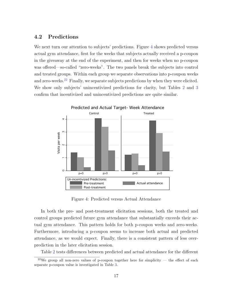
We next turn our attention to subjects’ predictions. Figure 4 shows predicted versus

actual gym attendance, first for the weeks that subjects actually received a p-coupon

in the giveaway at the end of the experiment, and then for weeks when no p-coupon

was offered—so-called “zero-weeks”. The two panels break the subjects into control

and treated groups. Within each group we separate observations into p-coupon weeks

and zero-weeks.22 Finally, we separate subjects predictions by when they were elicited.

We show only subjects’ unincentivized predictions for clarity, but Tables 2 and 3

confirm that incentivized and unincentivized predictions are quite similar.

01

23

4

p=0 p>0 p=0 p>0

Control Treated

Pre-treatment Actual attendance

Visit

s pe

r wee

k

Predicted and Actual Target- Week Attendance

Un-incentivized Predictions:

Post-treatment

Figure 4: Predicted versus Actual Attendance

In both the pre- and post-treatment elicitation sessions, both the treated and

control groups predicted future gym attendance that substantially exceeds their ac-

tual gym attendance. This pattern holds for both p-coupon weeks and zero-weeks.

Furthermore, introducing a p-coupon seems to increase both actual and predicted

attendance, as we would expect. Finally, there is a consistent pattern of less over-

prediction in the later elicitation session.

Table 2 tests differences between predicted and actual attendance for the different

22We group all non-zero values of p-coupon together here for simplicity — the effect of eachseparate p-coupon value is investigated in Table 3.

17

groups and elicitation sessions, pooled over values of the p-coupon. The first column

of each panel looks at predictions as captured by subjects’ p-coupon bids. The second

and third refer to their unincentivized predictions, for p-coupon weeks and zero-weeks.

In all cases subjects significantly over-predict future gym attendance, by as much as

two visits per week. It is particularly striking that subjects substantially over-predict

gym attendance in weeks with no p-coupon, suggesting that the overprediction is not

driven by the p-coupon incentives. On the basis of these results we can rule out, in

our model, both time consistency (β = 1) and full sophistication (β = β) if, after the

treatment, subjects have rational expectations over their future costs.

Table 2: Misprediction of attendanceControl group Treatment group

Bid Pred Pred Bid Pred Predp > 0 p > 0 p = 0 p > 0 p > 0 p = 0

Pre-Treatment PredictionsPredicted attendance 3.868 4.053 1.418 3.63 3.963 1.231Actual attendance 1.561 1.561 0.255 1.463 1.463 0.365Difference 2.307 2.491 1.164 2.167 2.500 0.865St. Error (0.297) (0.235) (0.149) (0.350) (0.318) (0.178)No. of observations 57 57 55 54 54 52

Post-Treatment PredictionsPredicted attendance 3.395 3.614 1.058 3.185 3.056 1.313Actual attendance 1.561 1.561 0.269 1.463 1.463 0.396Difference 1.833 2.053 0.788 1.722 1.593 0.917St. Error (0.321) (0.299) (0.144) (0.315) (0.299) (0.171)No. of observations 57 57 52 54 54 48

Notes: Bid includes only observations for a subject’s incentivized week. Pred in-cludes is separated into this week and the unincentivized week for which subjectswere asked to make predictions without a p-coupon.

In Table 3 we explore the effect of p-coupon value, and the change in predictions

over time. The first column regresses actual attendance on dummies for the various

values of p-coupon.23 The point estimates on the p-value dummies indicate a nearly

monotonic effect of monetary incentives, and pairwise comparisons of the coefficients

do not reject monotonicity. This is reassuring, as it suggests an upward-sloping labor

23The omitted category is p = $7 throughout this table. This is so that we can compare coefficientsacross ’Actual’ and ’Pred’ (for each of which the lowest value is p = $0), and ’Bid’ (where the lowestvalue is p = $1). In addition, all specifications in this table include individual covariates.

18

supply curve, as we would expect. The second and third columns regress bids and

unincentivized predictions on the same p-coupon dummies, plus a dummy for the

post-treatment elicitation session. Subjects appear to predict the slope of their labor-

supply curve relatively accurately, despite consistently over-predicting its intercept.

Table 3: Predictions: Delay versus Session Effects(1) (2) (3) (4) (5)

Actual Bid Pred Bid Pred

Sessiona -0.630∗∗∗ -0.707∗∗∗ -0.476∗∗ -0.810∗∗∗

(0.132) (0.112) (0.226) (0.187)p=$0 -2.275∗∗∗ -3.360∗∗∗ -3.925∗∗∗

(0.611) (0.498) (0.598)p=$1 -1.669∗∗ -0.924 -1.650∗∗∗ -0.512 -1.618∗∗

(0.689) (0.581) (0.482) (1.235) (0.640)p=$2 -1.304∗ -0.760 -1.288∗∗∗ -1.522 -2.213∗∗∗

(0.708) (0.579) (0.478) (1.232) (0.617)p=$3 -1.440∗∗ -0.530 -0.924∗ -0.489 -1.276∗∗

(0.714) (0.580) (0.472) (1.233) (0.634)p=$5 -0.050 -0.081 -0.272 0.027 -0.698

(0.808) (0.623) (0.523) (1.241) (0.648)Constant 2.600∗∗∗ 3.865∗∗∗ 4.953∗∗∗ 3.988∗∗∗ 5.405∗∗∗

(0.609) (0.613) (0.497) (1.233) (0.590)Observations 551 875 1088 176 217R-squared 0.20 0.06 0.27 0.11 0.33Num Clusters: 111 111 111 110 111Sample Full Full Full 5-wk delay 5-wk delay

Notes: aPre=0, Post=1. Robust standard errors in parentheses, clustered by indi-vidual. ∗ significant at 10%; ∗∗ significant at 5%; ∗∗∗ significant at 1%. p = $7 isthe omitted category.

The session dummy implies that, between the first and second elicitation sessions,

subjects reduce their predictions by roughly two-thirds of a visit per week. These

sessions differ in two ways: they are a month apart in time, and the second session

is closer to the target weeks than the first. One possibility is that subjects’ discount

factors decrease smoothly over time rather than abruptly as in the beta–delta model.

If so, we would see a change in mispredictions merely because the temporal proximity

of the target weeks is greater in the post-treatment elicitation session. We can examine

this by comparing first-session predictions for the first target week with second-session

predictions for the fifth target week. This comparison holds temporal proximity

19

constant. Columns (4) and (5) report the results of this regression. The coefficients

on the session dummy, for both bids and unincentivized predictions, still show a

substantial decrease in over-prediction over time. Apparently something neither we

nor the subjects foresaw is happening between the second and sixth weeks of the

semester that is causing subjects to lower their predictions of future gym attendance

by half to two-thirds of a visit per week. This suggests that there is systematic

misprediction along more than one dimension of the gym-attendance decision. One

possibility is that subjects begin the semester with overly optimistic beliefs about

their amount of free time in the semester, and become more realistic as the semester

unfolds.24

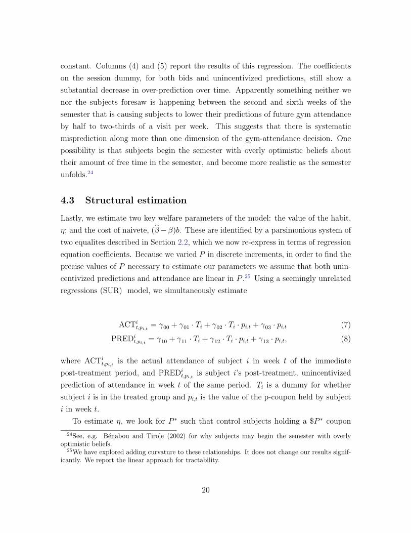
4.3 Structural estimation

Lastly, we estimate two key welfare parameters of the model: the value of the habit,

η; and the cost of naivete, (β−β)b. These are identified by a parsimonious system of

two equalites described in Section 2.2, which we now re-express in terms of regression

equation coefficients. Because we varied P in discrete increments, in order to find the

precise values of P necessary to estimate our parameters we assume that both unin-

centivized predictions and attendance are linear in P .25 Using a seemingly unrelated

regressions (SUR) model, we simultaneously estimate

ACTit,pi,t

= γ00 + γ01 · Ti + γ02 · Ti · pi,t + γ03 · pi,t (7)

PREDit,pi,t

= γ10 + γ11 · Ti + γ12 · Ti · pi,t + γ13 · pi,t, (8)

where ACTit,pi,t

is the actual attendance of subject i in week t of the immediate

post-treatment period, and PREDit,pi,t

is subject i’s post-treatment, unincentivized

prediction of attendance in week t of the same period. Ti is a dummy for whether

subject i is in the treated group and pi,t is the value of the p-coupon held by subject

i in week t.

To estimate η, we look for P ∗ such that control subjects holding a $P ∗ coupon

24See, e.g. Benabou and Tirole (2002) for why subjects may begin the semester with overlyoptimistic beliefs.

25We have explored adding curvature to these relationships. It does not change our results signif-icantly. We report the linear approach for tractability.

20

attend the gym as much as unincentivized treatment subjects. We can now re-express

these group means in terms of regression coefficients:

ACTT

t,0 = γ00 + γ01 = γ00 + γ03 · P ∗ = ACTC

t,p∗ (9)

Solving for P ∗, and hence for η, we get η = P ∗ = γ01/γ03.

To estimate (β − β)b we want P ∗ such that control subjects holding a $P coupon

predict the level of attendance actually achieved by a $P ∗ coupon:26

PREDC

t,ep = γ10 + γ13 · P = γ00 + γ03 · P ∗ = ACTC

t,p∗ . (10)

To implement this we substitute P , the average value of P in the control group, for

P . Solving this for P ∗ − P , and hence for (β − β)b, we get (β − β)b = P ∗ − P =

[γ10 − γ00 + (γ13 − γ03)P ]/γ03

Table 4 shows the results of the two-equation SUR system, and, beneath these,

the estimates of the structural parameters of interest. The left-hand panel shows the

results when we include the entire treated group. The right-hand panel restricts the

sample to include only those treated subjects whose attendance increased by at least

one visit per week, our so-called habit formers.

Our estimate of the “cost of naivete” is $3.91. This is the portion of the future

benefit of a single gym visit that present bias will cause subjects to forego, and that

naivete will cause them to think they will not forego. Put another way, it is the

difference, on average, between the dollar value a fully sophisticated subject would

put on a 100% effective gym-attendance commitment device, and the dollar value our

subjects would put on such a device. It is important to note that this estimate of

foregone future benefit does not depend upon any assumptions about the long-term

benefits of gym attendance, but is based entirely on subjects’ own evaluation of the

long-term benefits. Our estimate of the dollar value of the habit-formation effect

among the treated group is $0.40, suggesting that the $100 per subject treatment

incentive increased average gym-attendance utility by the monetary equivalent of

forty cents per visit. While this average effect informs the overall cost-effectiveness of

the intervention, it masks the heterogeneity of the treatment we observed in Section

26Note that we are using post-treatment unincentivized predictions, which, given our results insection 4.2, we assume are based on correct beliefs about target-week costs. Our model equallyallows us to use pre-treatment unincentivized predictions, given the greater over-prediction in thefirst session, we choose the more conservative option.

21

Table 4: Parameter EstimationAll Subjects Controls and Habit-Formers(1) (2) (3) (4)

ACT PRED ACT PRED

SUR ResultsTreatment Group 0.180∗ 0.062 2.020∗∗∗ 1.155∗∗

(0.106) (0.245) (0.205) (0.499)Treated X $P -0.138∗∗ -0.173∗∗ -0.128 0.013

(0.066) (0.084) (0.245) (0.176)$P 0.447∗∗∗ 0.558∗∗∗ 0.448∗∗∗ 0.565∗∗∗

(0.047) (0.058) (0.045) (0.059)Constant 0.259∗∗∗ 1.684∗∗∗ 0.258∗∗∗ 1.670∗∗∗

(0.074) (0.170) (0.071) (0.170)Observations 545 545 320 320Parameter EstimatesHabit Value, η 0.403∗ 4.505∗∗∗

(0.230) (0.603)

Cost of Naivete, (β − β)b 3.913∗∗∗ 3.906∗∗∗

(0.694) (0.688)Standard errors in parentheses. * significant at 10%; ** significantat 5%; *** significant at 1%

22

4.1. If we inflate the habit-value estimate in the full sample by the inverse of the

proportion of habit-formers in the treatment group we get a back-of-the-envelope

estimate of $3.11 for the habit value among habit formers.

To address habit-formation heterogeneity in a different way the right-hand panel of

Table 4 confines the analysis to just those treated subjects identified as habit-formers

and estimates the value of their habit. Among treated subjects whose immediate

post-treatment attendance increased by at least one visit per week, we find a habit

value of $4.51, much larger than the average for the entire treated group27, while the

cost of naivete remains roughly unchanged. These results depend on the assumption

that, after controlling for observables, those in the control group who would have

formed a habit respond in the same way to a p-coupon as those who would not have

formed a habit. In appendix A.6 we explore the differences in covariates between

the habit-formers and non habit-formers in the treatment group, and we are reas-

sured by the fact that their observed behavior responds identically to p-coupons.28

The only covariate on which they differ significantly is self-reported importance of

physical fitness, which is higher among habit-formers. This might help to explain

why they formed a habit. But it is hard to see how it would affect their response

to the p-coupons, suggesting that this difference may not be a problem for our es-

timation strategy. However, because we are comparing the habit-formers against all

control subjects—rather than only those who would have formed habits had they

been treated—these columns should not be treated with the same confidence as our

other results.

5 Conclusion

We find that incentivizing gym-attendance creates a short-run habit that is smaller

than, but statistically indistinguishable from, Charness and Gneezy’s (2009) effect,

and which decays substantially as the result of an exogenous break in attendance.

Although Charness and Gneezy find, at most, very slow decay, a model that incor-

porates short-term shocks to the cost of gym attendance can rationalize both their

27But similar to inflating the aggregate habit-value by the inverse of the compliance rate.28In a regression comparing p-responsiveness between habit-formers and non habit-formers (not

shown), the coefficients on the p-coupon value differ only by a statistically insignificant −0.039. Itis not clear why this comparison should be different between the comparable subjects in the controlgroup.

23

findings and ours. Our findings can be explained by the four-week common shock of

winter break, while a much slower path of decay would result from a series of smaller,

independent shocks over a longer period of time.29

Furthermore, we find that subjects have self-control problems of the sort generated

by present bias, and that they are at least partially naive with respect to these self-

control problems. Even in weeks with no p-coupon to complicate the prediction

task, subjects over-predict attendance by about one visit per week—a factor of about

three. This is a sufficient degree of mis-prediction to explain the result in DellaVigna

and Malmendier (2006) that people purchase monthly health club memberships when

their actual attendance only justifies the purchase of single-visit passes.30

Because they may be partially, rather than completely, naive about their future

self-control problems, we cannot take subjects’ predictions as statements of their true

preferences, and thus we cannot estimate the full cost of their self-contol problems.

However, we are able to estimate the portion of foregone future benefits that they fail

to predict—approximately $4—which serves as a lower bound on the foregone future

benefits, and hence on the total future benefits. We also find that for subjects who

form a habit, the habit-formation effect almost exactly offsets this cost of naivete. In

a population of “procrastinators” who initially believe that, in expectation, they will

attend the gym in the future but do not attend in the current period, this term is

also the minimum increase in gym-attendance utility necessary to induce attendance

(in expectation).

In addition to these results on naive self-control problems, we are able to rule

out that the decrease in over-prediction over the course of the treatment month is

caused by the increased temporal proximity of outcomes, as would be predicted by a

model of true hyperbolic discounting—as opposed to the quasi-hyperbolic discounting

captured by the beta–delta model. Instead it appears that subjects’ predictions may

become more accurate because they are learning something about the distribution of

gym-attendance costs as the semester unfolds. We interpret this as being consistent

with the literature on overoptimism, but do not propose a specific explanation. Our

data also allow us to explore whether subjects predict the habit-formation effect itself,

although this topic is beyond the scope of this paper.

29It seems reasonable that a habit that can be induced by a positive four-week shock can beeliminated by a negative four-week shock.

30DellaVigna and Malmendier (2006) consider a very different population, of course, so we do notclaim that this is driving their result.

24

We found an average habit-formation effect among treated subjects (who complied

with the protocol) of approximately one-third of a visit per week, though this effect

is heavily concentrated in the upper tail of the distribution. From the standpoint

of public policy it is this local average treatment effect that matters because non-

compliers do not incur the cost of the treatment incentive. We estimate the unforeseen

portion of long-term benefits that treated subjects’ self-control problems cause them

to forego at roughly four dollars. The overall long-term benefits, therefore, must

be at least this much. Adding to this approximately $0.50 for the average habit

value among compliers, we can establish a rough upper bound of sixty-nine weeks

on how long the habit would have to persist in order to break even on the cost of

the incentive.31 If the incentive could have been targeted to those we identified as

forming a habit, the break-even decay horizon would be just forty-six weeks. In our

sample of students, however, we see significant decay after winter break, suggesting

that exogenous interruptions in attendance may undermine the intervention. One

must also exercise caution in extrapolating these results to other populations, where

compliance, habit formation, and habit decay might all be quite different.

Our design also allows us to address the source of gym attendance motivation.

Gneezy and Rustichini (2000) argue that introducing small financial incentives may,

counterintuitively, reduce a behavior by crowding out intrinsic motivation. We find

no evidence that this is the case for gym attendance, either for our main treatment

intervention or for our smaller post-treatment incentives. We find that a temporary

subsidy increases attendance both while it is in place and in the short run after its

removal. We also find that both treated and control subjects respond positively to

the incentives provided by our p-coupons. A direct comparison of average attendance

during coupon weeks and zero weeks among the treated group strongly rejects the null

that unincentivized attendance is higher (p = 0.0004). Moreover, we cannot reject

that attendance is monotonically increasing in p-coupon value.32 While intrinsic

motivation may still be reduced by our financial incentives, it does not appear to be

of first-order significance for our results.

31This is an upper bound because we do not know the true long-term benefit, which may besubstantially higher than just the portion foregone due to self-control problems. We simply dividethe expected cost of the intervention ($100 multiplied by the 80% compliance rate) by the weeklybenefits ($4.50 multiplied by the 0.256 visits/week treatment effect).

32That is, for no pair of adjacent coupon values is attendance for recipients of the smaller couponstatistically greater than attendance for recipients of the larger. We do not reject monotonicity ineither the full sample or within either experimental group.

25

Future research should explore the habit-formation and habit-decay effects in a

more policy-relevant population. Subjects might be selected on the basis of health

risks such as obesity, and efforts could be made to select true procrastinators. In

addition, effort should be made to try to identify the ex-ante determinants of habit

formation so that incentives can be more effectively targeted. For example, we find

that treatment subjects who ultimately developed a habit had initially expressed

stronger beliefs that fitness was important, despite no difference in initial gym at-

tendance. The issue of subjects’ predictions also warrants further study, including

the critical issue of predicting the habit-formation effect, for which a larger sample is

necessary.

References

Becker, Gary and Kevin Murphy, “A Theory of Rational Addiction,” Journalof Political Economy, August 1988, 96 (4), 675–700.

Benabou, Roland and Jean Tirole, “Self-Confidence and Personal Motivation,”The Quarterly Journal of Economics, August 2002, 117 (3), 871–915.

Charness, Gary and Uri Gneezy, “Incentives to Exercise,” Econometrica, May2009, 77 (3), 909–931.

DellaVigna, Stefano and Ulrike Malmendier, “Contract Design and Self-Control: Theory and Evidence,” The Quarterly Journal of Economics, May2004, 119 (2), 353–402.

and , “Paying Not To Go To The Gym,” The American Economic Review,June 2006, 96 (3), 694–719.

Gelbach, Jonah, “When Do Covariates Matter? And Which Ones, and HowMuch?,” Working Paper, June 2009.

Gneezy, Uri and Aldo Rustichini, “Pay Enough, or Don’t Pay at All,” TheQuarterly Journal of Economics, August 2000, 115 (3), 791–810.

Kane, Robert, Paul Johnson, Robert Town, and Mary Butler, “A Struc-tured Review of the Effect of Economic Incentives on Consumers’ PreventiveBehavior,” American Journal of Preventive Medicine, 2004, 27 (4).

Laibson, David, “Golden Eggs and Hyperbolic Discounting,” The Quarterly Journalof Economics, May 1997, 112 (2), 443–477.

26

O’Donoghue, Ted and Matthew Rabin, “Addiction and Self Control,” in JonElster, ed., Addiction: Entries and Exits, Russel Sage Foundation, 1999.

and , “Doing It Now or Later,” The American Economic Review, March1999, 89 (1), 103–124.

Phelps, Edmund and Robert Pollak, “On Second-Best National Savings andGame-Equilibrium Growth,” The Review of Economic Studies, April 1968, 35(2), 185–199.

Zellner, Arnold, “An Efficient Method of Estimating Seemingly Unrelated Regres-sions and Tests for Aggregation Bias,” Journal of the American Statistical As-sociation, June 1962, 57 (298), 348–368.

27

A Appendices

A.1 Sample

Our initial sample consisted of 120 subjects, randomly assigned to treated and controlgroups of 60 subjects each. Table 5 provides a comparison of the treated and controlgroups. Due to attrition and missing covariates the final number of treated subjectsin our analysis is 54 and of control subjects 57. Comparing the two groups on thecovariates that we used in all of our analysis we find no significant differences inmeans, and the F-test of joint significance of the covariates in a linear regression ofthe treatment-group dummy on covariates is 0.387. In addition to basic demographicvariables we included discretionary budget and the time and money cost of gettingto campus in order to control for differences in the cost of gym attendance and therelative value of monetary incentives. The pre-treatment Godin Activity Scale is aself-reported measure of physical activity in a typical week prior to the treatment. Theself-reported importance of physical fitness and physical appearance were included asa proxy for subjects’ taste for the outcomes typically associated with gym-attendance.The naivete proxy covariates are subjects answers to a series of questions that we askedin order to assess their level of sophistication about self-control problems. Answerswere given on a four-point scale from “Disagree Strongly” to “Agree Strongly”. Theexact wording of these questions is as follows:

Variable QuestionForget I often forget appointments or plans that I’ve made, so

that I either miss them, or else have to rearrange myplans at the last minute.

Spontaneous I often do things spontaneously without planning.

Things come up I often have things come up in my life that cause me tochange my plans.

Think ahead I typically think ahead carefully, so I have a pretty goodidea what I’ll be doing in a week or a month.

Procrastinate I usually want to do things I like right away, but put offthings that I don’t like.

28

Table 5: Comparison of Treated and Control groups.(1) (2) (3) (4)

Full sample Treated group Control group T-test p-valueOriginal sample 120 60 60No. of attriters 6 4 2No. w/ incomplete controls 3 2 1Final sample size 111 54 57$25 learning-week incentive Yes Yes$100 treatment-month incentive Yes –Demographic covariates

Age 21.919 22.204 21.649 0.639(0.586) (0.990) (0.658)

Gender (1=female) 0.685 0.648 0.719 0.425(0.044) (0.066) (0.060)

Proportion white 0.36 0.333 0.386 0.568(0.046) (0.065) (0.065)

Proportion Asian 0.559 0.63 0.491 0.145(0.047) (0.066) (0.067)

Proportion other race 0.081 0.037 0.123 0.01(0.026) (0.026) (0.044)

Economic covariatesDiscretionary budget 192.342 208.333 177.193 0.404

(18.560) (28.830) (23.749)Travel cost to campus 0.901 0.648 1.14 0.37

(0.273) (0.334) (0.428)Travel time to campus (min) 14.662 14.398 14.912 0.811

(1.071) (1.703) (1.335)Naivete proxy covariates

Forgeta,b 1.595 1.556 1.632 0.573(0.067) (0.090) (0.099)

Spontaneousa,b 2.486 2.574 2.404 0.281(0.079) (0.104) (0.117)

Things come upa,b 2.586 2.611 2.561 0.731(0.072) (0.107) (0.097)

Think aheada,b 2.874 2.944 2.807 0.338(0.071) (0.081) (0.116)

Procrastinatea,b 3.036 3.056 3.018 0.8(0.075) (0.104) (0.108)

Exercise experience and attitude covariatesPre-trt Godin Activity Scale 36.05 36.5 35.623 0.855

(2.376) (2.983) (3.689)Fitness is importanta,b 3.081 2.981 3.175 0.092

(0.057) (0.086) (0.076)Appearance is importanta,b 3.252 3.259 3.246 0.917

(0.065) (0.096) (0.088)F-test of joint significance 0.387

Notes: a 1= Disagree Strongly, 2=Disagree Somewhat; 3=Agree Somewhat;4=Agree Strongly. b Wording of questions in appendix. Standard errors in paren-theses.

29

A.2 Screening mechanism

The webpage we used to screen for non-attenders is shown below. We included three“dummy” questions to make it harder for subjects to return to the site and changetheir answers in order to be able to join the experiment. Despite this precaution,a handful of subjects may have returned to the screening site and modified theiranswers until they hit upon the correct answer to join the experiment. (Which wasa “no” on question four.) Out of a total of 497 unique IP addresses in our screeninglog, we found 5 instances of subjects possibly gaming the system to gain access to thestudy. We have no way to determine if these subjects wound up in our subject pool.

Figure 5: Screening Site

30

A.3 Elicitation mechanisms

Figure 6 depicts the sample p-coupon and instructions that subjects saw to preparethem for the incentive-compatible elicitation task. Verbal instructions given at thistime further clarified exactly what we were asking subjects to do. Note that the sure-thing values in column A are increments of $P . The line number where subjects crossover from choosing column B to choosing column A bounds their valuation for thep-coupon. We used a linear interpolation between these bounds to create our “BDM”variable. Thus, for example, if a subject chose B at and below line four, and thenchose A at and above line five we assigned them a p-coupon valuation of $P × 4.5 Ingeneral subjects appear to have understood this task clearly. There were only threesubjects who failed to display a single crossing on every task, and all of them appearto have realized what they were doing before the end of the first elicitation session.The observations for which these three subjects did not display a single crossing havebeen dropped from our analysis.

By randomly choosing only one target week for only one subject we maintainincentive compatibility while leaving all but one subject per session actually holdinga p-coupon, and for only one target week. This is important because what we careabout is the change in their valuation of a p-coupon from pre- to post-treatmentelicitation sessions. Subjects who are already holding a coupon from the first sessionwould be valuing a second coupon in the second session, making their valuationspotentially incomparable, rather like comparing willingness-to-pay for a first candybar to willingness-to-pay for a second candy bar.

The instructions and example for the unincentivized prediction task and the taskfor prediction of other people’s attendance appear as figure 7.

31

[PRACTICE]

This exercise involves nine questions, relating to the Daily RSF-Reward Certificate shown at the top of the page. Each question gives you two options, A or B. For each question check the option you prefer.

You will be asked to complete this exercise four times, once each for four of the five target weeks. The daily value of the certificate will be different for each of these four target weeks. For one of the five weeks you will not be asked to complete this exercise.

At the end of the session I’ll choose one of the five target weeks at random. Then I’ll choose one of the nine questions at random. Then I’ll choose one subject at random. The randomly chosen subject will receive whichever option they checked on the randomly chosen question for the randomly chosen target week. Thus, for each question it is in your interest to check the option you prefer.

For each question, check which option you prefer, A or B.

Option A Option B

1. Would you prefer $1 for certain,

paid Monday, Oct 20. or The Daily RSF-Reward Certificate

shown above.



shown above.



shown above.



shown above.



shown above.



shown above.



shown above.



shown above.



shown above.

Page 3

S M T W T F S SEPT 1 2 3 4 5 6

7 8 9 10 11 12 13 14 15 16 17 18 19 20 21 22 23 24 25 26 27

OCT 28 29 30 1 2 3 4 5 6 7 8 9 10 11 12 13 14 15 16 17 18 19 20 21 22 23 24 25

NOV 26 27 28 29 30 31 1 2 3 4 5 6 7 8 9 10 11 12 13 14 15 16 17 18 19 20 21 22 23 24 25 26 27 28 29

Daily RSF-Reward Certificate

This certificate entitles the holder to $1

for every day that he or she attends the RSF during the week of

Monday, Oct 13 through Sunday, Oct 19.

$1 $1

$1 $1

Figure 6: Sample p-coupon and incentive-compatible elicitation task

32

[PRACTICE]

For each target week you will also be asked to complete the following two exercises. Both of these exercises relate to the Daily RSF-Reward Certificate shown at the top of the page, which is the same as the one shown at the top of the preceding page. In addition, there will be one target week for which you will be shown no certificate, and you will be asked to complete only these last two exercises.

Imagine that you have just been given the Daily RSF-Reward Certificate shown above, and that this is

the only certificate you are going to receive from this experiment.

How many days would you attend the RSF that week if you had been given that certificate? ______

Now imagine that everyone in the room except you has just been given the Daily RSF-Reward Certificate

shown above, and that this is the only certificate they are going to receive from this experiment.

What do you think would be the average number of days the other people in the room (not including

you) would go to the RSF that week? _______

(Your answer does not have to be a round number. It can be a fraction or decimal.)

Notes: As part of this experiment some subjects will receive real certificates.

I will give a $10 prize to the subject whose answer to this exercise is closest to the correct,

average RSF-attendance for subjects (other than themselves) who receive the certificate

shown above. The prize money will be paid by check, mailed on Monday,.Oct 20.

Page 4

S M T W T F S SEPT 1 2 3 4 5 6

7 8 9 10 11 12 13 14 15 16 17 18 19 20 21 22 23 24 25 26 27

OCT 28 29 30 1 2 3 4 5 6 7 8 9 10 11 12 13 14 15 16 17 18 19 20 21 22 23 24 25

NOV 26 27 28 29 30 31 1 2 3 4 5 6 7 8 9 10 11 12 13 14 15 16 17 18 19 20 21 22 23 24 25 26 27 28 29

Daily RSF-Reward Certificate

This certificate entitles the holder to $1

for every day that he or she attends the RSF during the week of

Monday, Oct 13 through Sunday, Oct 19.

$1 $1

$1 $1

Figure 7: Unincentivized and other elicitation tasks

33

A.4 Compliance, attrition, and randomization.

About 80% of Charness and Gneezy’s high-incentive subjects complied with the $100treatment incentive by attending the gym eight times during the treatment month.A similar percentage, 75%, of our treatment subjects complied with our treatmentincentive by attending the gym twice a week during the treatment month. In ourdata, a direct comparison of means between treatment and control will only allowus to estimate an “intention to treat” effect (ITT). If compliance were random wecould simply inflate this by the inverse of the compliance rate to estimate the averagetreatment effect. Since compliance is almost certainly not random, we will do ourbest to estimate an “average treatment effect on the treated” (ATT) by using ourrich set of individual covariates to help us control for differences between compliersand non-compliers.

To mitigate attrition over our three sessions we gave subjects two participationpayments of $25 each, in addition to the various gym-attendance offers. The firstpayment was for attendance at the first session. The second payment required atten-dance at both the second and third sessions.33 Despite this titration of rewards, six ofthe 120 subjects did not complete the study. Two control subjects and two treatmentsubjects left the study between the first and second sessions, and two more treatmentsubjects left between the second and third. In order to include an additional handfulof subjects who were not able to make the third session, and otherwise would haveleft the study, we held make-up sessions the following day. Four control subjects andtwo treatment subjects attended these sessions and we have treated them as havingcompleted the study.

Randomizing subjects into treatment and control presented some challenges. Ourdesign required that treatment and control subjects meet separately. For each of thethree sessions we scheduled four timeslots, back-to-back, and staggered them betweenControl and Treatment. When subjects responded to the online solicitation, and afterthey had completed the screening questionnaire, they were randomly assigned toeither treatment or control and were then asked to choose between the two timeslotsallocated to their assigned group. Subjects who could not find a timeslot that fittheir schedule voluntarily left the study at this point.34 As it turned out, subjectsassigned to the treatment group were substantially less likely to find a timeslot thatworked for them, and as a result the desired number of subjects were successfullyenrolled in the control group well before the treatment group was filled. Wanting topreserve the balanced number of Treatment and Control subjects, maintain powerto identify heterogeneity within the Treatment group, and stay within the budgetfor the study, we capped the control group and continued to solicit participants inorder to fill the treatment group. Subjects who responded to the solicitation after the

33Gym-attendance offers were not tied to attendance because this would have created a differentialbetween the treatment and control groups in the incentive to complete the study.

34Technically they were considered to have never joined the study, and received no payment.

34

Control group was filled were randomly assigned to treatment or control, and thoseassigned to control were then thanked and told that the study was full. Our treatmentgroup therefore includes subjects who were either solicited later, or responded to thesolicitation later than any of the subjects in the control group.35

To the extent that these temporal differences are correlated with any of the be-haviors we are studying, simple comparisons of group averages may be biased. Itappears, however, that the two groups are not substantially different along any ofthe dimensions we observed in our dataset, as a joint F-test does reject that the twogroups were randomly selected from the same population based on observables. Acomparison of the two groups appears in a separate appendix. To address the pos-sibility that they may have differed significantly on unobservables we use observablecontrols in our hypothesis tests.

35Additionally, the two groups of subjects were available at different times of day. To the extentthat what made it hard for Treatment subjects to find a timeslot that fit the schedule may havebeen correlated with gym-attendance behavior (if, for example, the Treatment timeslots happen tohave coincided with the most prefered times for non-gym exercise), then the group averages for someoutcome variables may be biased.

35

Table 6: Comparison of Compliers and Non-Compliers(1) (2) (3) (4)

Treated Group Compliers Non-Compliers T-test p-valueDemographic covariates

Age 22.204 22.605 20.636 0.429(0.990) (1.234) (0.472)

Gender (1=female) 0.648 0.651 0.636 0.929(0.066) (0.074) (0.152)








Forgeta,b 1.556 1.465 1.909 0.047(0.090) (0.096) (0.211)

Spontaneousa,b 2.574 2.442 3.091 0.011(0.104) (0.101) (0.285)

Things come upa,b 2.611 2.558 2.818 0.333(0.107) (0.101) (0.352)

Think aheada,b 2.944 2.977 2.818 0.436(0.081) (0.091) (0.182)





(0.096) (0.095) (0.304)N obs. 54 43 11F-test of joint significance 0.635


36

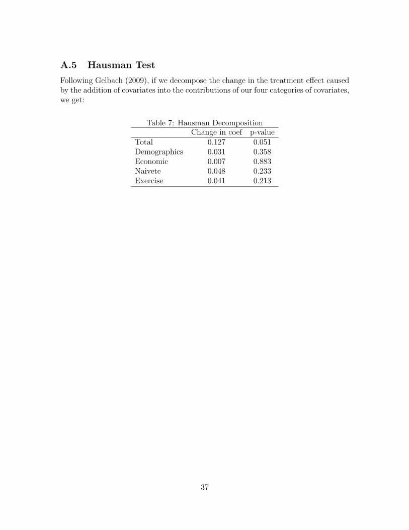
A.5 Hausman Test

Following Gelbach (2009), if we decompose the change in the treatment effect causedby the addition of covariates into the contributions of our four categories of covariates,we get:

Table 7: Hausman DecompositionChange in coef p-value

Total 0.127 0.051Demographics 0.031 0.358Economic 0.007 0.883Naivete 0.048 0.233Exercise 0.041 0.213

37

A.6 Habit Formers

38

Table 8: Comparison of Habit-Formers and Non Habit-Formers(1) (2) (3) (4)

Treated Group “Habit-Formers” Non Habit-Formers T-test p-valueDemographic covariates

Age 22.204 19.750 22.630 0.306(0.990) (0.453) (1.150)

Gender (1=female) 0.648 0.625 0.652 0.885(0.066) (0.183) (0.071)








Forgeta,b 1.556 1.500 1.565 0.800(0.090) (0.327) (0.091)

Spontaneousa,b 2.574 2.250 2.630 0.198(0.104) (0.164) (0.118)

Things come upa,b 2.611 2.375 2.652 0.363(0.107) (0.263) (0.117)

Think aheada,b 2.944 3.000 2.935 0.778(0.081) (0.189) (0.090)





(0.096) (0.183) (0.109)N obs. 54 8 46F-test of joint significance 0.663


39

Habit Formation and Naivet e in Gym Attendance: …...Habit Formation and Naivet e in Gym...

Documents

Transcript of Habit Formation and Naivet e in Gym Attendance: …...Habit Formation and Naivet e in Gym...