H2 optimal model order reduction for parametric systems ... Sarah... · MAX PLANCK INSTITUTE FOR...
53
MAX PLANCK INSTITUTE FOR DYNAMICS OF COMPLEX TECHNICAL SYSTEMS MAGDEBURG August, 2013 NLA and Optimization Workshop Vancouver H 2 optimal model order reduction for parametric systems using RBF metamodels Peter Benner, Sara Grundel, Nils Hornung MPI Magdeburg and Fraunhofer SCAI Max Planck Institute Magdeburg Grundel, MOR and RBF 1/34
Transcript of H2 optimal model order reduction for parametric systems ... Sarah... · MAX PLANCK INSTITUTE FOR...

MAX PLANCK INSTITUTE
FOR DYNAMICS OF COMPLEX
TECHNICAL SYSTEMS
MAGDEBURG
August, 2013NLA and Optimization Workshop
Vancouver
H2 optimal model order reduction forparametric systems using RBF metamodels
Peter Benner, Sara Grundel, Nils HornungMPI Magdeburg and Fraunhofer SCAI
Max Planck Institute Magdeburg Grundel, MOR and RBF 1/34

H2 MOR Parametric MOR Numerik Medium Model
Abstract
Model Order ReductionModel Order Reduction Methods for linear systems are well studiedand many successful methods exist. We will review some andexplain more recent advances inParametric Model Order Reduction. The focus will be on methodswhere we interpolate certain significant measures, that arecomputed for specific values of the parameter byRadial Basis Function Interpolation. These measures have adisadvantage as they behave like eigenvalues of matrices dependingon parameters and we will explain how that can be dealt with inpractice. We will furthermore need to introduce a technique tocreate a medium size model.
Model Order Reduction
Max Planck Institute Magdeburg Grundel, MOR and RBF 2/34
H2 MOR Parametric MOR Numerik Medium Model
Abstract
Model Order Reduction Methods for linear systems are well studiedand many successful methods exist. We will review some andexplain more recent advances inParametric Model Order ReductionParametric Model Order Reduction. The focus will be on methodswhere we interpolate certain significant measures, that arecomputed for specific values of the parameter byRadial Basis Function InterpolationRadial Basis Function Interpolation . These measures have adisadvantage as they behave like eigenvalues of matrices dependingon parameters and we will explain how that can be dealt with inpractice. We will furthermore need to introduce a technique tocreate a medium size model.
Parametric Model Order Reduction
Radial Basis Function Interpolation
Max Planck Institute Magdeburg Grundel, MOR and RBF 2/34
H2 MOR Parametric MOR Numerik Medium Model
Abstract
Model Order Reduction Methods for linear systems are well studiedand many successful methods exist. We will review some andexplain more recent advances inParametric Model Order Reduction. The focus will be on methodswhere we interpolate certain significant measures, that arecomputed for specific values of the parameter byRadial Basis Function Interpolation. These measures have adisadvantage as they behave like eigenvalues of matrices dependingon parameters and we will explain how that can be dealt with inpractice. We will furthermore need to introduce a technique tocreate a medium size model.medium size model.medium size model.
Max Planck Institute Magdeburg Grundel, MOR and RBF 2/34

H2 MOR Parametric MOR Numerik Medium Model
Outline
1 H2 MOR
2 Parametric MOR
3 Numerik
4 Medium Model
Max Planck Institute Magdeburg Grundel, MOR and RBF 3/34

H2 MOR Parametric MOR Numerik Medium Model
What is MOR?
Max Planck Institute Magdeburg Grundel, MOR and RBF 4/34

H2 MOR Parametric MOR Numerik Medium Model
Projection-Based MOR
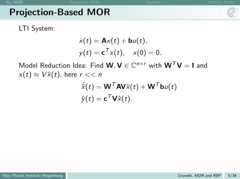
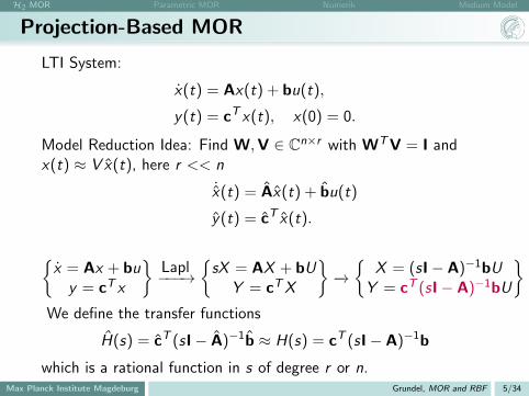
LTI System:
x(t) = Ax(t) + bu(t),
y(t) = cT x(t), x(0) = 0.
Model Reduction Idea: Find W,V ∈ Cn×r with WTV = I andx(t) ≈ V x(t), here r << n
WTV ˙x(t) = WTAVx(t) + WTbu(t)
y(t) = cTVx(t).
{x = Ax + buy = cT x
}Lapl−−−→
{sX = AX + bU
Y = cTX
}−→{
X = (sI− A)−1bUY = cT (sI− A)−1bU
}(1)
We define the transfer functions
H(s) = cT (sI− A)−1b ≈ H(s) = cT (sI− A)−1b
which is a rational function in s of degree r or n.
Max Planck Institute Magdeburg Grundel, MOR and RBF 5/34
H2 MOR Parametric MOR Numerik Medium Model
Projection-Based MOR
LTI System:
x(t) = Ax(t) + bu(t),
y(t) = cT x(t), x(0) = 0.
Model Reduction Idea: Find W,V ∈ Cn×r with WTV = I andx(t) ≈ V x(t), here r << n
WTV
˙x(t) = WTAVx(t) + WTbu(t)
y(t) = cTVx(t).
{x = Ax + buy = cT x
}Lapl−−−→
{sX = AX + bU
Y = cTX
}−→{
X = (sI− A)−1bUY = cT (sI− A)−1bU
}(1)
We define the transfer functions
H(s) = cT (sI− A)−1b ≈ H(s) = cT (sI− A)−1b
which is a rational function in s of degree r or n.
Max Planck Institute Magdeburg Grundel, MOR and RBF 5/34

H2 MOR Parametric MOR Numerik Medium Model
Projection-Based MOR
LTI System:
x(t) = Ax(t) + bu(t),
y(t) = cT x(t), x(0) = 0.
Model Reduction Idea: Find W,V ∈ Cn×r with WTV = I andx(t) ≈ V x(t), here r << n
WTV
˙x(t) = Ax(t) + bu(t)
y(t) = cT x(t).
{x = Ax + buy = cT x
}Lapl−−−→
{sX = AX + bU
Y = cTX
}−→{
X = (sI− A)−1bUY = cT (sI− A)−1bU
}(1)
We define the transfer functions
H(s) = cT (sI− A)−1b ≈ H(s) = cT (sI− A)−1b
which is a rational function in s of degree r or n.
Max Planck Institute Magdeburg Grundel, MOR and RBF 5/34
H2 MOR Parametric MOR Numerik Medium Model
Projection-Based MOR
LTI System:
x(t) = Ax(t) + bu(t),
y(t) = cT x(t), x(0) = 0.
Model Reduction Idea: Find W,V ∈ Cn×r with WTV = I andx(t) ≈ V x(t), here r << n
WTV
˙x(t) = Ax(t) + bu(t)
y(t) = cT x(t).
{x = Ax + buy = cT x
}Lapl−−−→
{sX = AX + bU
Y = cTX
}−→{
X = (sI− A)−1bUY = cT (sI− A)−1bU
}(1)
We define the transfer functions
H(s) = cT (sI− A)−1b ≈ H(s) = cT (sI− A)−1b
which is a rational function in s of degree r or n.Max Planck Institute Magdeburg Grundel, MOR and RBF 5/34

H2 MOR Parametric MOR Numerik Medium Model
H2 Model Order Reduction
Good Reduced Order Model{u
Σ−→ y
uΣ−→ y
}‖y − y‖ small
We know that:
supt≥0|y(t)− y(t)| ≤ ‖H − H‖H2‖u‖L2 .
for ‖H − H‖H2 :=(
12π
∫∞−∞ |H(ιω)− H(ιω)|2dω
)1/2.
References[Absil, Antoulas, Baur, Beattie, Benner, Breiten,
Bunse-Gerstner, Gallivan, Gugercin, Kubalinska, Van Dooren,
Vossen, Wilczek,... ]
Max Planck Institute Magdeburg Grundel, MOR and RBF 6/34
H2 MOR Parametric MOR Numerik Medium Model
H2 Model Order Reduction
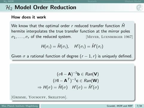
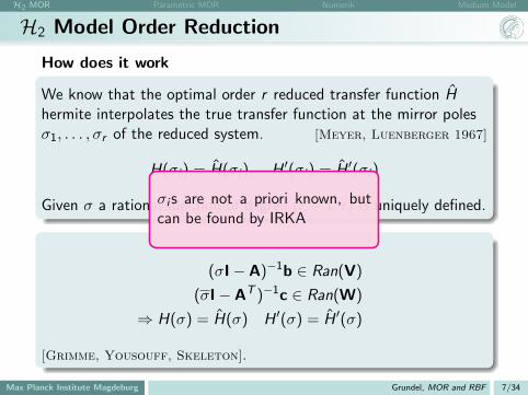
How does it work
We know that the optimal order r reduced transfer function Hhermite interpolates the true transfer function at the mirror polesσ1, . . . , σr of the reduced system. [Meyer, Luenberger 1967]
H(σi ) = H(σi ), H ′(σi ) = H ′(σi )
Given σ a rational function of degree (r − 1, r) is uniquely defined.
(σI− A)−1b ∈ Ran(V)
(σI− AT )−1c ∈ Ran(W)
⇒ H(σ) = H(σ) H ′(σ) = H ′(σ)
[Grimme, Yousouff, Skeleton].
σi s are not a priori known, butcan be found by IRKA
Max Planck Institute Magdeburg Grundel, MOR and RBF 7/34
H2 MOR Parametric MOR Numerik Medium Model
H2 Model Order Reduction
How does it work
We know that the optimal order r reduced transfer function Hhermite interpolates the true transfer function at the mirror polesσ1, . . . , σr of the reduced system. [Meyer, Luenberger 1967]
H(σi ) = H(σi ), H ′(σi ) = H ′(σi )
Given σ a rational function of degree (r − 1, r) is uniquely defined.
(σI− A)−1b ∈ Ran(V)
(σI− AT )−1c ∈ Ran(W)
⇒ H(σ) = H(σ) H ′(σ) = H ′(σ)
[Grimme, Yousouff, Skeleton].
σi s are not a priori known, butcan be found by IRKA
Max Planck Institute Magdeburg Grundel, MOR and RBF 7/34

H2 MOR Parametric MOR Numerik Medium Model
IRKA [Antoulas,Beattie,Gugercin 2006]
Algorithm 1 Iterative rational Krylov algorithm (IRKA)
Input: Initial selection of interpolation points σi , closed under con-jugation and a convergence tolerance tol .
Output: A, b, c1: Choose V and W s.t. range (V) = {(σ1I − A)−1b, . . . , (σr I −
A)−1b} and range (W) = {(σ1I−AT )−1c, . . . , (σr I−AT )−1c}and WTV = I.
2: while relative change in {σi} > tol do3: A = WTAV,4: assign σi ← −λi (A) for i = 1, . . . , r ,5: update V and W s.t. range (V) = {(σ1I−A)−1b, . . . , (σr I−
A)−1b} and range (W) = {(σ1I − AT )−1c, . . . , (σr I −AT )−1c} and WTV = I.
6: end while7: A = WTAV, b = WTb, cT = cTV
Max Planck Institute Magdeburg Grundel, MOR and RBF 8/34

H2 MOR Parametric MOR Numerik Medium Model
Outline
1 H2 MOR
2 Parametric MOR
3 Numerik
4 Medium Model
Max Planck Institute Magdeburg Grundel, MOR and RBF 9/34

H2 MOR Parametric MOR Numerik Medium Model
Parametrized Dynamical System
LTI System: (p ∈ P ⊂ Rp)
x(t) = A(p)x(t) + b(p)u(t),
y(t) = c(p)T x(t), x(0) = 0.
Model Reduction:
˙x(t) = A(p)x(t) + b(p)u(t)
y(t) = c(p)T x(t)
This means that the approximated transfer function
H(s, p) = c(p)T (sI−A(p))−1b(p) ≈ H(s, p) = c(p)T (sI−A(p))−1b(p)
is a rational function in s, but also a function in p.
Max Planck Institute Magdeburg Grundel, MOR and RBF 10/34

H2 MOR Parametric MOR Numerik Medium Model
Previous Work
Reduced matrices from original matrices
A(p)→ A(p) c(p)→ c(p) b(p)→ b(p) (2)
Many attempt for parameteric Model Order Reduction exist
projection matrix independent of parameterA = V TA(p)WA = V TA(p)W[Breiten,Damm,Baur,Benner,Beattie, Gugercin]
matrix interpolationA(pi )A(pi )[Panzer et al] or [Amsallam, Farhat]
transfer function interpolationH(si , pj)H(si , pj)[Antoulas, Ionita]
A = V TA(p)W
A(pi )
H(si , pj)
Max Planck Institute Magdeburg Grundel, MOR and RBF 11/34

H2 MOR Parametric MOR Numerik Medium Model
PMOR and H2
Knowing σ1(p), . . . , σr (p) seems to be crucial
With that we can create the reduced order model viaprojection
We would then get the reduced order system that minimizes
‖H(p)− H(p)‖H2
for each p.
Idea
⇒ metamodelling of σi (p).
Problem
Is this even a function? How smooth?
Max Planck Institute Magdeburg Grundel, MOR and RBF 12/34
H2 MOR Parametric MOR Numerik Medium Model
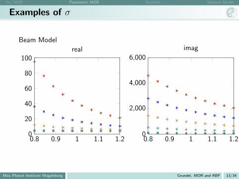
Examples of σ
Beam Model
0.8 0.9 1 1.1 1.20
20
40
60
80
100real
0.8 0.9 1 1.1 1.20
2,000
4,000
6,000
imag
Max Planck Institute Magdeburg Grundel, MOR and RBF 13/34

H2 MOR Parametric MOR Numerik Medium Model
Examples of σ
Convection Diffusion Model
0 0.2 0.4 0.6 0.8 10
1,000
2,000
3,000real
0.2 0.4 0.6 0.8 1−1
−0.5
0
0.5
1
imag
Max Planck Institute Magdeburg Grundel, MOR and RBF 13/34

H2 MOR Parametric MOR Numerik Medium Model
Examples of σ
Anemometer
0 0.2 0.4 0.6 0.8 10
1
2
3
4
5·104 real
0 0.2 0.4 0.6 0.8 1−1
−0.5
0
0.5
1
imag
Max Planck Institute Magdeburg Grundel, MOR and RBF 13/34

H2 MOR Parametric MOR Numerik Medium Model
Synthetic Example
10−3 10−2 10−1 100 101−1,000
0
1,000
2,000
3,000real
10−3 10−2 10−1 100 101−1,000
−500
0
500
1,000
imag
Max Planck Institute Magdeburg Grundel, MOR and RBF 14/34

H2 MOR Parametric MOR Numerik Medium Model
Synthetic Example
10−3 10−2 10−1 100 101−1,000
−500
0
500
1,000
imag
10−3 10−2 10−1 100 101−1,000
0
1,000
2,000
3,000real
Max Planck Institute Magdeburg Grundel, MOR and RBF 14/34

H2 MOR Parametric MOR Numerik Medium Model
2D Example
Scanning Electrochemical Microscopy
5 0 5
0.2
0.4
real
0 5 100
510
−0.50
0.5
imag
0 5 10 0510−0.5
0
0.5
0 5 10 05100
0.2
0.4
Max Planck Institute Magdeburg Grundel, MOR and RBF 15/34
H2 MOR Parametric MOR Numerik Medium Model
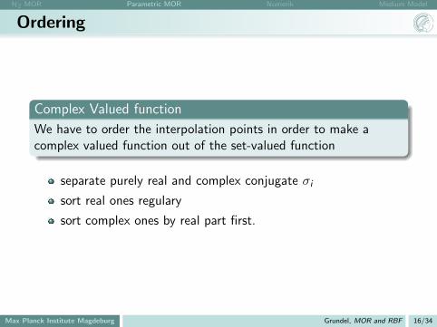
Ordering
Complex Valued function
We have to order the interpolation points in order to make acomplex valued function out of the set-valued function
separate purely real and complex conjugate σi
sort real ones regulary
sort complex ones by real part first.
Max Planck Institute Magdeburg Grundel, MOR and RBF 16/34

H2 MOR Parametric MOR Numerik Medium Model
Metamodelling using k means
in most applications the σi behave quit nicely
create metamodels for different clusters (clustering)
given p1, . . . , pN consider tuples
(C1pi , σ(pi ),C2ni ) ∈ Rp × Cr × N
where ni measures the number of real values and1 < C1 < C2.
k means1 Set initial means for all K clusters
2 assign each tuple to the cluster with the nearest mean
3 Calculate new mean
4 repeat until convergence
Max Planck Institute Magdeburg Grundel, MOR and RBF 17/34

H2 MOR Parametric MOR Numerik Medium Model
Radial Basis Interpolation
Ansatz
Given p1, . . . , pN and function values σ(p1), . . . , σ(pN) theinterpolant is created by
σ(p) =∑
γiR(‖p − pi‖)
where R(x) = exp(−θx2)
simple interpolation technique
θ found problem dependent
γi found by solving a linear system (interpolation condition)
different model for each cluster
Max Planck Institute Magdeburg Grundel, MOR and RBF 18/34
H2 MOR Parametric MOR Numerik Medium Model
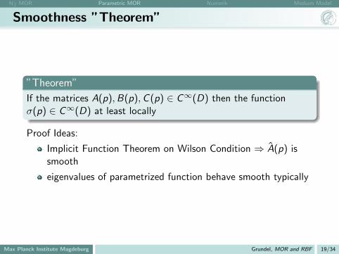
Smoothness ”Theorem”
”Theorem”
If the matrices A(p),B(p),C (p) ∈ C∞(D) then the functionσ(p) ∈ C∞(D) at least locally
Proof Ideas:
Implicit Function Theorem on Wilson Condition ⇒ A(p) issmooth
eigenvalues of parametrized function behave smooth typically
Max Planck Institute Magdeburg Grundel, MOR and RBF 19/34

H2 MOR Parametric MOR Numerik Medium Model
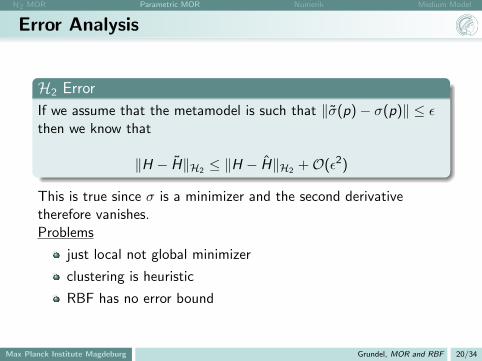
Error Analysis
H2 Error
If we assume that the metamodel is such that ‖σ(p)− σ(p)‖ ≤ εthen we know that
‖H − H‖H2 ≤ ‖H − H‖H2 +O(ε2)
This is true since σ is a minimizer and the second derivativetherefore vanishes.
Problems
just local not global minimizer
clustering is heuristic
RBF has no error bound
Max Planck Institute Magdeburg Grundel, MOR and RBF 20/34
H2 MOR Parametric MOR Numerik Medium Model
Error Analysis
H2 Error
If we assume that the metamodel is such that ‖σ(p)− σ(p)‖ ≤ εthen we know that
‖H − H‖H2 ≤ ‖H − H‖H2 +O(ε2)
This is true since σ is a minimizer and the second derivativetherefore vanishes.Problems
just local not global minimizer
clustering is heuristic
RBF has no error bound
Max Planck Institute Magdeburg Grundel, MOR and RBF 20/34

H2 MOR Parametric MOR Numerik Medium Model
Outline
1 H2 MOR
2 Parametric MOR
3 Numerik
4 Medium Model
Max Planck Institute Magdeburg Grundel, MOR and RBF 21/34
H2 MOR Parametric MOR Numerik Medium Model
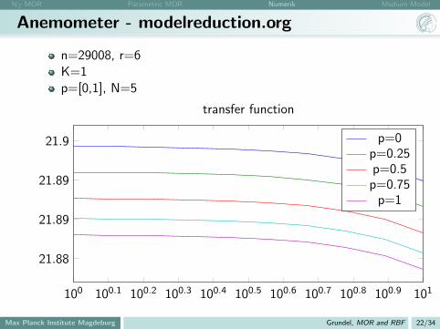
Anemometer - modelreduction.org
n=29008, r=6K=1p=[0,1], N=5
100 100.1 100.2 100.3 100.4 100.5 100.6 100.7 100.8 100.9 101
21.88
21.89
21.89
21.9
transfer function
p=0p=0.25p=0.5
p=0.75p=1
Max Planck Institute Magdeburg Grundel, MOR and RBF 22/34

H2 MOR Parametric MOR Numerik Medium Model
Anemometer - modelreduction.org
0 0.1 0.2 0.3 0.4 0.5 0.6 0.7 0.8 0.9 110−3
10−2
IRKAinterpolated
‖H‖H2 ≈ 2.7e4
Max Planck Institute Magdeburg Grundel, MOR and RBF 22/34
H2 MOR Parametric MOR Numerik Medium Model
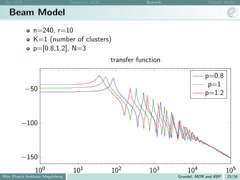
Beam Model
n=240, r=10K=1 (number of clusters)p=[0.8,1.2], N=3
100 101 102 103 104 105
−150
−100
−50
transfer function
p=0.8p=1
p=1.2
Max Planck Institute Magdeburg Grundel, MOR and RBF 23/34

H2 MOR Parametric MOR Numerik Medium Model
Beam Model
0.8 0.85 0.9 0.95 1 1.05 1.1 1.15 1.2
10−8
10−7
H2 Error
interpolatedIRKA
‖H‖H2 ≈ 0.0035
Max Planck Institute Magdeburg Grundel, MOR and RBF 23/34

H2 MOR Parametric MOR Numerik Medium Model
Synthetic
n=100, r=10K=4p=[0,1],N=50
100 101 102 103
−20
−15
−10
−5
transfer function
p=0.25p=5
p=0.75p=1
Max Planck Institute Magdeburg Grundel, MOR and RBF 24/34

H2 MOR Parametric MOR Numerik Medium Model
Synthetic
0 0.1 0.2 0.3 0.4 0.5 0.6 0.7 0.8 0.9 110−10
10−7
10−4
10−1
102
H2 Error
interpolatedIRKA
‖H‖H2 ≈ 10
Max Planck Institute Magdeburg Grundel, MOR and RBF 24/34

H2 MOR Parametric MOR Numerik Medium Model
On-line versus Off-line
Off-line
precomputation
time is not so important
possible bigger computing resources
On-line
simulate the reduced order model for different parameter orinput functions
computing time crucial
phase 1: compute the reduced state space system
phase 2: simulate it (system size r is crucial)
Max Planck Institute Magdeburg Grundel, MOR and RBF 25/34

H2 MOR Parametric MOR Numerik Medium Model
Anemometer Timings
N=5 (number of interpolation points in parameter domain)
the error of the interpolated and projected function is veryclose to the error of a reduced order model computed byIRKA directly
Depending on the application this may however beproblematic timewise.
Example r=4 r=6 r=10
create σ model 86s 122 s 382sone IRKA run 43s 150s 216sdo the projection 3s 4.8s 8s
Max Planck Institute Magdeburg Grundel, MOR and RBF 26/34

H2 MOR Parametric MOR Numerik Medium Model
Outline
1 H2 MOR
2 Parametric MOR
3 Numerik
4 Medium Model
Max Planck Institute Magdeburg Grundel, MOR and RBF 27/34
H2 MOR Parametric MOR Numerik Medium Model
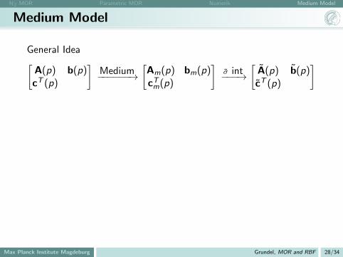
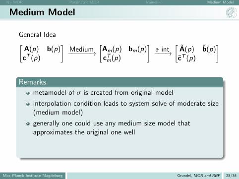
Medium Model
General Idea[A(p) b(p)cT (p)
]Medium−−−−−−→
[Am(p) bm(p)cTm(p)
]σ int−−−→
[A(p) b(p)cT (p)
]
Remarks
metamodel of σ is created from original model
interpolation condition leads to system solve of moderate size(medium model)
generally one could use any medium size model thatapproximates the original one well
V is created such that the medium size model interpolates atmany points in frequency and parameter
Max Planck Institute Magdeburg Grundel, MOR and RBF 28/34
H2 MOR Parametric MOR Numerik Medium Model
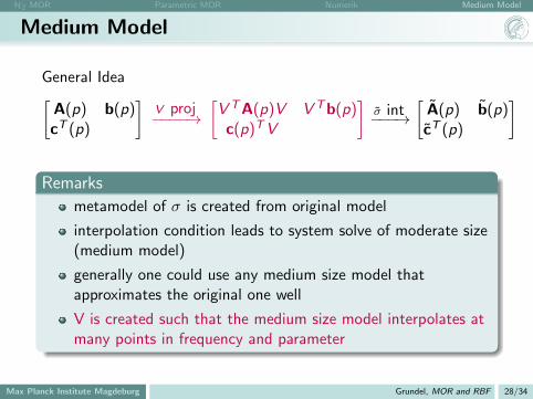
Medium Model
General Idea[A(p) b(p)cT (p)
]V proj−−−−→
[V TA(p)V V Tb(p)
c(p)TV
]σ int−−−→
[A(p) b(p)cT (p)
]
Remarks
metamodel of σ is created from original model
interpolation condition leads to system solve of moderate size(medium model)
generally one could use any medium size model thatapproximates the original one well
V is created such that the medium size model interpolates atmany points in frequency and parameter
Max Planck Institute Magdeburg Grundel, MOR and RBF 28/34

H2 MOR Parametric MOR Numerik Medium Model
Algorithm
Algorithm 2 Offline Phase Calculation
1: Pick parameter points p1, . . . , pN2: for i = 1 to N do3: Compute via IRKA σ(pi ) and Vi ,Wi projection matrices4: end for5: Create metamodel6: Compute V from all Vi and Wi
7: Precompute medium size matrices with V
Max Planck Institute Magdeburg Grundel, MOR and RBF 29/34
H2 MOR Parametric MOR Numerik Medium Model
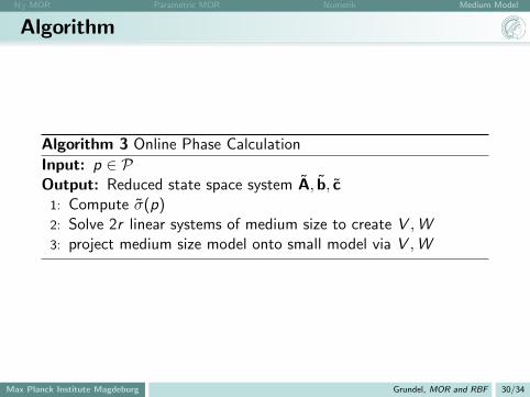
Algorithm
Algorithm 3 Online Phase Calculation
Input: p ∈ POutput: Reduced state space system A, b, c1: Compute σ(p)2: Solve 2r linear systems of medium size to create V ,W3: project medium size model onto small model via V ,W
Max Planck Institute Magdeburg Grundel, MOR and RBF 30/34

H2 MOR Parametric MOR Numerik Medium Model
Error Bounds
Lemma [Higham 2004, Grundel-Benner 2013]
Assuming that ‖H − Hm‖∞ ≤ ε‖H‖∞ and σ1, . . . , σr giveninterpolation points. If Hr interpolates H and Hm
r interpolates Hm
then‖Hr − Hm
r ‖ ≤ (ε+ δ + εδ)‖Hr‖+ δ‖Hmr ‖
where δ =∑∞
k=1(‖L‖‖L−1‖ε)k
This is basically related to forward stability of rationalinterpolation.
Lij =
{H(σi (p),p)−H(σj (p),p)
σi (p)−σj (p) if i 6= j∂∂σH(σi (p), p) if i = j
}
Max Planck Institute Magdeburg Grundel, MOR and RBF 31/34
H2 MOR Parametric MOR Numerik Medium Model
Comparison
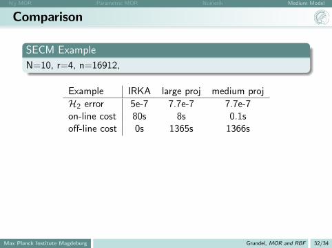
SECM Example
N=10, r=4, n=16912,
Example IRKA large proj medium proj
H2 error 5e-7 7.7e-7 7.7e-7on-line cost 80s 8s 0.1soff-line cost 0s 1365s 1366s
The medium model itelf is not a good approximation but itsprojection on almost optimal points is close to the true best.
online cost is just to cost to create the reduced order model,not to simulate anything.
off-line cost is cost to create the metamodel and medium sizemodel (severel IRKA runs mainly)
Max Planck Institute Magdeburg Grundel, MOR and RBF 32/34
H2 MOR Parametric MOR Numerik Medium Model
Comparison
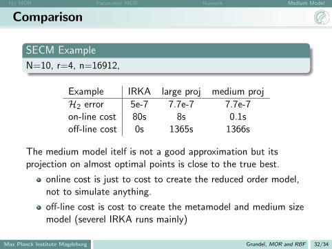
SECM Example
N=10, r=4, n=16912,
Example IRKA large proj medium proj
H2 error 5e-7 7.7e-7 7.7e-7on-line cost 80s 8s 0.1soff-line cost 0s 1365s 1366s
The medium model itelf is not a good approximation but itsprojection on almost optimal points is close to the true best.
online cost is just to cost to create the reduced order model,not to simulate anything.
off-line cost is cost to create the metamodel and medium sizemodel (severel IRKA runs mainly)
Max Planck Institute Magdeburg Grundel, MOR and RBF 32/34

H2 MOR Parametric MOR Numerik Medium Model
Summary
1 introduction to H2 Model Order Reduction
2 new approach to Parametric Model Order Reduction usingRBFs
3 the direct method needs some extra online computation time
4 medium model can reduce that to a small amount
5 some open problems in clustering, related to the smoothnessof the function σ
Max Planck Institute Magdeburg Grundel, MOR and RBF 33/34
H2 MOR Parametric MOR Numerik Medium Model
Thank you
Max Planck Institute Magdeburg Grundel, MOR and RBF 34/34

H2 MOR Parametric MOR Numerik Medium Model
Thank you
Max Planck Institute Magdeburg Grundel, MOR and RBF 34/34

H2 MOR Parametric MOR Numerik Medium Model
Thank you
Max Planck Institute Magdeburg Grundel, MOR and RBF 34/34