H-INFINITY FILTERING VIA LMI APPROACH AND ITS APPLICATION

ROBUST AND REDUCED ORDER H-INFINITY FILTERING VIA LMI APPROACH AND ITS APPLICATION TO FAULT DETECTION 425

ROBUST AND REDUCED ORDER H-INFINITY FILTERING VIA LMI APPROACH AND ITS APPLICATION TO FAULT DETECTION

Young-Man Kim and John M. Watkins

x

ROBUST AND REDUCED ORDER H-INFINITY FILTERING VIA LMI

APPROACH AND ITS APPLICATION TO FAULT DETECTION

Young-Man Kim and John M. Watkins

Department of Electrical Engineering and Computer Science, Wichita State University United States of America

1. Introduction

Filters that estimate the state variables of a system are important tools for control and signal processing applications. Early work in the area assumed that the system dynamics were known and external disturbances were white noise with known statistical properties. In contrast to traditional Kalman filters, H filters do not require knowledge of the statistical properties of the noise. H filters are more robust to disturbances and modeling uncertainties than Kalman filters. Thus, in practical applications where disturbances may not be known exactly and system uncertainties may appear in modeling, the H technique is often used (Fu et al., 1994). It is important to consider filter order when fast data processing is necessary. The reduced order filter is often desirable because it reduces the filter complexity and real time computational burdens in many applications. In (Grigoriadis & Watson, 1997) the reduced order H filtering problem was studied via an LMI (Linear Matrix Inequality) approach, but only for a specific linear time invariant plant model without model uncertainties. In (Bettayeb & Kavranoglu, 1994) the reduced order filter problem was studied in an H setting, but the H problem was formulated as distance problem. Because a wide variety of problems arising in system and control theory can be reduced to an optimization problem involving LMIs and LMIs can be solved numerically very efficiently, LMIs have been used extensively in the controls field. In (Tuan et al., 2000) the robust reduced order filtering problem was studied in an 2H setting via an LMI approach. In this study, the H approach is used because it is known that H approach is more robust to model uncertainties than 2H (Kim & Watkins, 2006). Less conservative results can be achieved, and a computational example is given to show this. This filtering technique can be used for fault detection filter design. As science and technology develops, the reliability and security of complex systems becomes more important. Thus, on-line monitoring of faults as they occur during operation of a dynamic

20

www.intechopen.com

Fault Detection426

system is necessary. In this study, estimator based fault detection methods will be the focus. The key to estimator based fault detection is to generate a fault indicating signal (residual) using input and output signals from the monitored system (Chen & Zhang, 1991). However, there is always a model-reality mismatch between plant dynamics and the model used for the residual generation (Chen & Patton, 1997). The robustness of residual depends on its fault sensitivity. The residual should be sensitive to faults but insensitive to modeling uncertainties and disturbances (Zhong et al., 2003). To produce the residual signal, an observer is usually used. In the fault detection literature this observer is often called a fault detection filter to emphasize the relationship with the filtering concept. In this study, robust fault detection filter (RFDF) design is formulated as a multi-objective H optimization for a polytopic uncertain system. In (Casavola et al., 2005a), RFDF design was formulated as a multi-objective H optimization only for the full order case. In (Casavola et al., 2005b), RFDF was formulated as a quasi-LMI only for the full order case. In this study, the order of the RFDF is reduced using LMI techniques and the detection performance is compared with the full order filter (Kim & Watkins, 2007). This paper is organized as follows: In Section 2, notations are introduced. In Section 3, the preliminary and main results for the H filter design are given. In Section 4, the preliminary and main results for the fault detection filter design are given. Numerical examples of H filter design and the fault detection filter design are shown in Section 5. Concluding remarks can be found in Section 6.

2. Notation

The notation that is used here is quite standard. R is the field of real numbers, nR is a real vector with dimension n and m nR is a real matrix with dimensions m n . RH is the subspace of L with real and rational functions that are analytic and bounded in the open right-half plane, where L is the set of functions bounded on j -axis including . TB is the transpose of matrix B. Symbol, *, stands for terms that are induced by symmetry,

e.g.,

(*) * T TT TS S S MK K

M Q M Q

BRL stands for Bounded Real Lemma, which is standard in robust control theory (Gahinet et al., 1996).

3. H Filter design

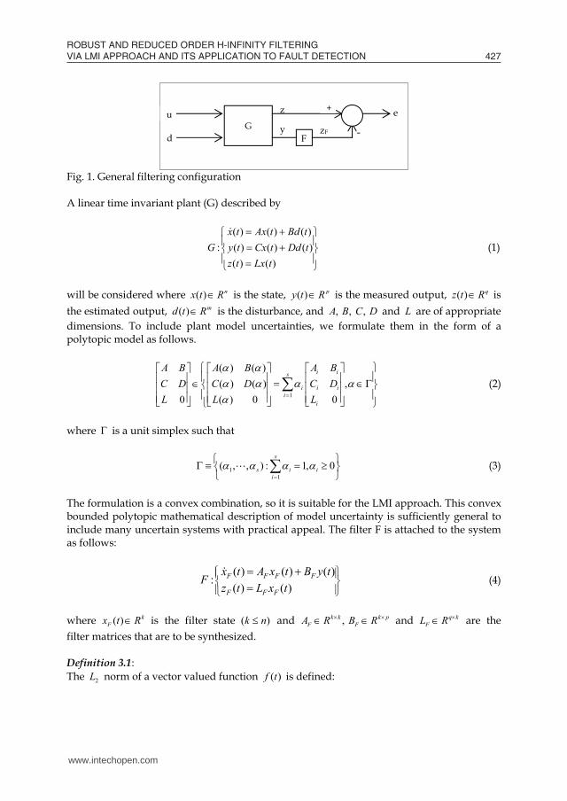
3.1 Preliminary result The general filtering configuration can be depicted as in Figure 1 where G is the plant, F is the filter that will be designed, d is an uncertain disturbance that includes process and measurement noise, z is the signal to be estimated, zF is the estimate of z, e is the estimation error, and y is the measured output.

Fig. 1. General filtering configuration

A linear time invariant plant (G) described by

( ) ( ) ( )

: ( ) ( ) ( )( ) ( )

x t Ax t Bd tG y t Cx t Dd t

z t Lx t

(1)

will be considered where ( ) nx t R is the state, ( ) py t R is the measured output, ( ) qz t R is the estimated output, ( ) md t R is the disturbance, and , , , A B C D and L are of appropriate dimensions. To include plant model uncertainties, we formulate them in the form of a polytopic model as follows.

1

( ) ( )( ) ( ) ,

0 ( ) 0 0

i is

i i ii

i

A B A B A BC D C D C DL L L

(2)

where is a unit simplex such that

11

( , , ) : 1, 0s

s i ii

(3)

The formulation is a convex combination, so it is suitable for the LMI approach. This convex bounded polytopic mathematical description of model uncertainty is sufficiently general to include many uncertain systems with practical appeal. The filter F is attached to the system as follows:

( ) ( ) ( ):

( ) ( )F F F F

F F F

x t A x t B y tF

z t L x t

(4)

where ( ) k

Fx t R is the filter state ( )k n and ,k k k pF FA R B R and q k

FL R are the filter matrices that are to be synthesized. Definition 3.1: The 2L norm of a vector valued function ( )f t is defined:

z

zF y

G F

u

d

e

-

+

www.intechopen.com


system is necessary. In this study, estimator based fault detection methods will be the focus. The key to estimator based fault detection is to generate a fault indicating signal (residual) using input and output signals from the monitored system (Chen & Zhang, 1991). However, there is always a model-reality mismatch between plant dynamics and the model used for the residual generation (Chen & Patton, 1997). The robustness of residual depends on its fault sensitivity. The residual should be sensitive to faults but insensitive to modeling uncertainties and disturbances (Zhong et al., 2003). To produce the residual signal, an observer is usually used. In the fault detection literature this observer is often called a fault detection filter to emphasize the relationship with the filtering concept. In this study, robust fault detection filter (RFDF) design is formulated as a multi-objective H optimization for a polytopic uncertain system. In (Casavola et al., 2005a), RFDF design was formulated as a multi-objective H optimization only for the full order case. In (Casavola et al., 2005b), RFDF was formulated as a quasi-LMI only for the full order case. In this study, the order of the RFDF is reduced using LMI techniques and the detection performance is compared with the full order filter (Kim & Watkins, 2007). This paper is organized as follows: In Section 2, notations are introduced. In Section 3, the preliminary and main results for the H filter design are given. In Section 4, the preliminary and main results for the fault detection filter design are given. Numerical examples of H filter design and the fault detection filter design are shown in Section 5. Concluding remarks can be found in Section 6.

2. Notation

The notation that is used here is quite standard. R is the field of real numbers, nR is a real vector with dimension n and m nR is a real matrix with dimensions m n . RH is the subspace of L with real and rational functions that are analytic and bounded in the open right-half plane, where L is the set of functions bounded on j -axis including . TB is the transpose of matrix B. Symbol, *, stands for terms that are induced by symmetry,

e.g.,

(*) * T TT TS S S MK K

M Q M Q

BRL stands for Bounded Real Lemma, which is standard in robust control theory (Gahinet et al., 1996).

3. H Filter design

3.1 Preliminary result The general filtering configuration can be depicted as in Figure 1 where G is the plant, F is the filter that will be designed, d is an uncertain disturbance that includes process and measurement noise, z is the signal to be estimated, zF is the estimate of z, e is the estimation error, and y is the measured output.

Fig. 1. General filtering configuration

A linear time invariant plant (G) described by

( ) ( ) ( )

: ( ) ( ) ( )( ) ( )

x t Ax t Bd tG y t Cx t Dd t

z t Lx t

(1)

will be considered where ( ) nx t R is the state, ( ) py t R is the measured output, ( ) qz t R is the estimated output, ( ) md t R is the disturbance, and , , , A B C D and L are of appropriate dimensions. To include plant model uncertainties, we formulate them in the form of a polytopic model as follows.

1

( ) ( )( ) ( ) ,

0 ( ) 0 0

i is

i i ii

i

A B A B A BC D C D C DL L L

(2)


11

( , , ) : 1, 0s

s i ii

(3)

The formulation is a convex combination, so it is suitable for the LMI approach. This convex bounded polytopic mathematical description of model uncertainty is sufficiently general to include many uncertain systems with practical appeal. The filter F is attached to the system as follows:

( ) ( ) ( ):

( ) ( )F F F F

F F F

x t A x t B y tF

z t L x t

(4)

where ( ) k

Fx t R is the filter state ( )k n and ,k k k pF FA R B R and q k

FL R are the filter matrices that are to be synthesized. Definition 3.1: The 2L norm of a vector valued function ( )f t is defined:

z

zF y

G F

u

d

e

-

+

www.intechopen.com

Fault Detection428

20

( ) ( )TL

f f t f t dt █ (5)

The goal of the H optimal filtering problem is to find a filter F to minimize the worst case estimation error energy

2Le over all bounded energy disturbance d, where Fe z z ,

that is

2

22

{0}min sup L

F d L L

e

d (6)

Using the induced 2L -gain property of the H norm, this problem is equivalent to the following H norm minimization problem

min edFT (7)

where edT is the transfer function from disturbance d to the estimation error e and the H norm is defined as the largest gain over all frequencies such that

max( ) sup ( ( ))ed edT s T j (8)

where max denotes maximum singular value of the given function. The -suboptimal H filtering problem is to find a filter F such that

edT (9)

where is a given positive scalar. To find the transfer function edT , (1) and (4) can be rewritten in augmented form as (10) and (11).

clF F F F

x Ax Bdx

x A x B y

= cl cl clA x B d (10)

cl F cl cle z z z L x (11) where

,clF

xx

x

0,cl

F F

AA

B C A ,cl

F

BB

B D and cl FL L L (12)

The transfer function of closed system, edT , can be found as:

cl cl cle z L x = 1( )cl cl clL sI A B d edT d (13)

where 1( )ed cl cl clT L sI A B (14) Using the well-known BRL (Gahinet & Apkarian, 1994), the condition in (9) with (14) can be described as:

0 00

T Tcl cl cl clTcl

cl

PA A P PB LB P IL I

(15)

where ,cl clA B and clL are given in (12) and P is a symmetric positive definite matrix variable. Equation (15) satisfies the design requirement as follows:

a) internal stability: for d=0, the state vector clx of closed loop system tends to zero as time goes to infinity.

b) performance: The H norm, edT , is less than specified positive scalar . Statement (a) implies quadratic stability and (b) implies quadratic performance. Remember that ,cl clA B and clL depend on parameter . Thus, statement (a) should be replaced by quadratic stability in the sense of parameter dependency and statement (b) replaced by quadratic performance in the sense of parameter dependency. Definition 3.2 (Gahinet et al., 1996): The system of (10) and (11) is said to have AQS (affine quadratic stability) if there exist a positive symmetric affine-parameter dependent Lyapunov matrix

1( )

s

i ii

P P

(16)

where , ( 1,2, , )iP i s are symmetric, such that

( ) ( ) ( ) ( ) 0,Tcl clA P P A █ (17)

Definition 3.3 (Gahinet et al., 1996): The system of (10) and (11) is said to have AQP (affine quadratic H performance) if there exists a positive symmetric affine-parameter dependent Lyapunov matrix (16) such that

( ) ( ) ( ) ( ) ( ) ( ) ( )( ) ( ) 0 0

( ) 0

T Tcl cl cl cl

Tcl

cl

A P P A P B LB P IL I

(18)

that holds for all admissible parameter ( 1,2, , )i i s █

www.intechopen.com


20

( ) ( )TL

f f t f t dt █ (5)

The goal of the H optimal filtering problem is to find a filter F to minimize the worst case estimation error energy

2Le over all bounded energy disturbance d, where Fe z z ,

that is

2

22

{0}min sup L

F d L L

e

d (6)

Using the induced 2L -gain property of the H norm, this problem is equivalent to the following H norm minimization problem

min edFT (7)

where edT is the transfer function from disturbance d to the estimation error e and the H norm is defined as the largest gain over all frequencies such that

max( ) sup ( ( ))ed edT s T j (8)

where max denotes maximum singular value of the given function. The -suboptimal H filtering problem is to find a filter F such that

edT (9)

where is a given positive scalar. To find the transfer function edT , (1) and (4) can be rewritten in augmented form as (10) and (11).

clF F F F

x Ax Bdx

x A x B y

= cl cl clA x B d (10)

cl F cl cle z z z L x (11) where

,clF

xx

x

0,cl

F F

AA

B C A ,cl

F

BB

B D and cl FL L L (12)

The transfer function of closed system, edT , can be found as:

cl cl cle z L x = 1( )cl cl clL sI A B d edT d (13)

where 1( )ed cl cl clT L sI A B (14) Using the well-known BRL (Gahinet & Apkarian, 1994), the condition in (9) with (14) can be described as:

0 00

T Tcl cl cl clTcl

cl

PA A P PB LB P IL I

(15)

where ,cl clA B and clL are given in (12) and P is a symmetric positive definite matrix variable. Equation (15) satisfies the design requirement as follows:

a) internal stability: for d=0, the state vector clx of closed loop system tends to zero as time goes to infinity.

b) performance: The H norm, edT , is less than specified positive scalar . Statement (a) implies quadratic stability and (b) implies quadratic performance. Remember that ,cl clA B and clL depend on parameter . Thus, statement (a) should be replaced by quadratic stability in the sense of parameter dependency and statement (b) replaced by quadratic performance in the sense of parameter dependency. Definition 3.2 (Gahinet et al., 1996): The system of (10) and (11) is said to have AQS (affine quadratic stability) if there exist a positive symmetric affine-parameter dependent Lyapunov matrix

1( )

s

i ii

P P

(16)

where , ( 1,2, , )iP i s are symmetric, such that

( ) ( ) ( ) ( ) 0,Tcl clA P P A █ (17)

Definition 3.3 (Gahinet et al., 1996): The system of (10) and (11) is said to have AQP (affine quadratic H performance) if there exists a positive symmetric affine-parameter dependent Lyapunov matrix (16) such that

( ) ( ) ( ) ( ) ( ) ( ) ( )( ) ( ) 0 0

( ) 0

T Tcl cl cl cl

Tcl

cl

A P P A P B LB P IL I

(18)

that holds for all admissible parameter ( 1,2, , )i i s █

www.intechopen.com

Fault Detection430

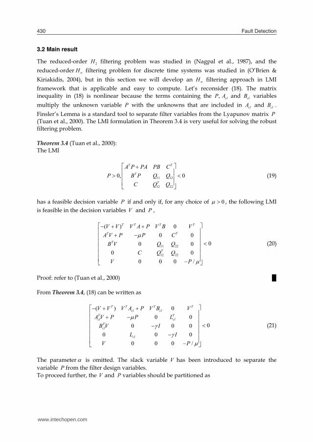
3.2 Main result

The reduced-order 2H filtering problem was studied in (Nagpal et al., 1987), and the reduced-order H filtering problem for discrete time systems was studied in (O’Brien & Kiriakidis, 2004), but in this section we will develop an H filtering approach in LMI framework that is applicable and easy to compute. Let’s reconsider (18). The matrix inequality in (18) is nonlinear because the terms containing the , clP A and clB variables multiply the unknown variable P with the unknowns that are included in clA and clB . Finsler’s Lemma is a standard tool to separate filter variables from the Lyapunov matrix P (Tuan et al., 2000). The LMI formulation in Theorem 3.4 is very useful for solving the robust filtering problem. Theorem 3.4 (Tuan et al., 2000): The LMI

11 12

12 22

0, 0

T T

T

T

A P PA PB CP B P Q Q

C Q Q

(19)

has a feasible decision variable P if and only if, for any choice of 0 , the following LMI is feasible in the decision variables V and P ,

11 22

12 22

( ) 00 0

00 00 0

0 0 0 /

T T T T

T T

T

T

V V V A P V B VA V P P CB V Q Q

C Q QV P

(20)

Proof: refer to (Tuan et al., 2000) █ From Theorem 3.4, (18) can be written as

( ) 00 0

00 0 00 0 0

0 0 0 /

T T T Tcl cl

T Tcl clTcl

cl

V V V A P V B VA V P P LB V I

L IV P

(21)

The parameter is omitted. The slack variable V has been introduced to separate the variable P from the filter design variables. To proceed further, the V and P variables should be partitioned as

11 12

21 22

V VV

V V (22)

1 3

3 2

TP PP

P P (23)

Because the reduced order case is being considered, the filter order k , will be less than or equal to the plant order n . The partitioned sub-matrices in (22) will be dimensionalized as

11( ),V n n 12( ),V n k 21( ),V k n and 22( )V k k . Now, we need to enforce some special structure on 21V as

21 21 ( )0k n kV V (24)

where 21V is a k k matrix. We can replace , , ,cl clV P A B and clL in (21) with (12), (22), (23) and (24). After that, we perform a congruence transformation with the transformation matrix

1 1 122 21 22 21 22 21diag I V V I V V I I I V V (25)

This yields (26)

11 11 2 1 11 1 3 11 11 1

1 1 2 3 2 2 2 1

1 3

2

1 3

2

ˆ ˆ( ) ( ) 0ˆˆ ˆ ˆ ˆ* ( ) 0

ˆ ˆ* * 0 0 0ˆ ˆ* * * 0 0 0

* * * * 0 0 0* * * * * 0 0

1 1ˆ ˆ* * * * * *

1 ˆ* * * * * * *

T T T T T T T TF F F

T TF F F

T T

TF

T

V V S S V A B C P A P V B B D V S

S S S A B C P A P S B B D S S

P P L

P LI

I

P P

P

0

(26)

where

1 21 22 21T TS V V V (27)

1 1 ( )0k n kS S (28)

2 21 22 12T T TS V V V (29)

21ˆ TF FB V B (30)

www.intechopen.com


3.2 Main result

The reduced-order 2H filtering problem was studied in (Nagpal et al., 1987), and the reduced-order H filtering problem for discrete time systems was studied in (O’Brien & Kiriakidis, 2004), but in this section we will develop an H filtering approach in LMI framework that is applicable and easy to compute. Let’s reconsider (18). The matrix inequality in (18) is nonlinear because the terms containing the , clP A and clB variables multiply the unknown variable P with the unknowns that are included in clA and clB . Finsler’s Lemma is a standard tool to separate filter variables from the Lyapunov matrix P (Tuan et al., 2000). The LMI formulation in Theorem 3.4 is very useful for solving the robust filtering problem. Theorem 3.4 (Tuan et al., 2000): The LMI

11 12

12 22

0, 0

T T

T

T

A P PA PB CP B P Q Q

C Q Q

(19)

has a feasible decision variable P if and only if, for any choice of 0 , the following LMI is feasible in the decision variables V and P ,

11 22

12 22

( ) 00 0

00 00 0

0 0 0 /

T T T T

T T

T

T

V V V A P V B VA V P P CB V Q Q

C Q QV P

(20)

Proof: refer to (Tuan et al., 2000) █ From Theorem 3.4, (18) can be written as

( ) 00 0

00 0 00 0 0

0 0 0 /

T T T Tcl cl

T Tcl clTcl

cl

V V V A P V B VA V P P LB V I

L IV P

(21)

The parameter is omitted. The slack variable V has been introduced to separate the variable P from the filter design variables. To proceed further, the V and P variables should be partitioned as

11 12

21 22

V VV

V V (22)

1 3

3 2

TP PP

P P (23)

Because the reduced order case is being considered, the filter order k , will be less than or equal to the plant order n . The partitioned sub-matrices in (22) will be dimensionalized as

11( ),V n n 12( ),V n k 21( ),V k n and 22( )V k k . Now, we need to enforce some special structure on 21V as

21 21 ( )0k n kV V (24)

where 21V is a k k matrix. We can replace , , ,cl clV P A B and clL in (21) with (12), (22), (23) and (24). After that, we perform a congruence transformation with the transformation matrix

1 1 122 21 22 21 22 21diag I V V I V V I I I V V (25)

This yields (26)

11 11 2 1 11 1 3 11 11 1

1 1 2 3 2 2 2 1

1 3

2

1 3

2

ˆ ˆ( ) ( ) 0ˆˆ ˆ ˆ ˆ* ( ) 0

ˆ ˆ* * 0 0 0ˆ ˆ* * * 0 0 0

* * * * 0 0 0* * * * * 0 0

1 1ˆ ˆ* * * * * *

1 ˆ* * * * * * *

T T T T T T T TF F F

T TF F F

T T

TF

T



P P L

P LI

I

P P

P

0

(26)

where

1 21 22 21T TS V V V (27)

1 1 ( )0k n kS S (28)

2 21 22 12T T TS V V V (29)

21ˆ TF FB V B (30)

www.intechopen.com

Fault Detection432

( )

ˆ

0F

Fn k p

BB

(31)

1 1P̂ P (32) 1

2 21 22 2 22 21ˆ T TP V V PV V (33)

13 3 22 21ˆT TP P V V (34)

121 22 21

ˆ TF FA V A V V (35)

( )

ˆ

0F

Fn k k

AA

(36)

122 21

ˆF FL L V V (37)

1 3

3 2

ˆ ˆˆ

ˆ ˆ

TP PP

P P

(38)

Remark 3.5: The H filtering solvability condition in (18) is reformulated as the feasibility problem of

(26) with respect to 1 2 11ˆ ˆ ˆ ˆ, , , , , , F F FA B L S S V P and where ˆ 0P . █

Remark 3.6: The filter matrices ,F FA B and FL can be derived by means of the following procedure.

(i) Compute 22V and 21V by solving the factorization problem 1

1 21 22 21TS V V V (39)

(ii) Compute ,F FA B and FL 1

21 21 22ˆT

F FA V A V V (40)

21ˆT

F FB V B (41) 1

21 22ˆ

F FL L V V █ (42) Now, we need to remember that we had a polytopic uncertain system. As explained in (Tuan et al., 2000), a parameter dependent Lyapunov matrix ( )P , such as

1( ) ( ),

s

i ii

P P

(43)

is symmetric positive definite for all admissible values of , if and only, if this holds for each iP . Therefore, we need to check the solvability of (18) only at the vertices, 1,2, ,i s . This gives us the final form (44) of the LMI (26).

11 11 2 1 11 1, 3, 11 11 1

1 1 2 3, 2, 2 2 1

1, 3,

2,

1,

ˆ ˆ( ) ( ) 0ˆˆ ˆ ˆ ˆ* ( ) 0

ˆ ˆ* * 0 0 0ˆ ˆ* * * 0 0 0

* * * * 0 0 0

* * * * * 0 0

1 1ˆ* * * * * *

T T T T T T T Ti F i i F i i F i

T Ti F i i F i i F i

T Ti i i

Ti F

i



P P L

P L

I

I

P

3,

2,

( 1, 2, , )

0

ˆ

1 ˆ* * * * * * *

Ti

i

i s

P

P

(44)

Consequently, the minimum upper bound for the reduced order H filter can be found by solving the LMI optimization problem

11 1 2ˆ ˆ ˆ ˆ, , , , , , ,min : (44)F F F iV S S A B L P (45)

In summary, the -suboptimal H reduced order filter for polytopic uncertain

system can be solved if and only if (44) holds for all vertices, 1,2, ,i s and the minimum value can be found from (45). Also, the triple ( , , )F F FA B L defining the thk order filter is obtained from (i) and (ii) in Remark 3.6.

4. Fault detection filter design

4.1 Preliminary result Let’s consider the following uncertain continuous time linear system described by

( ) ( ) ( ) ( ) ( ):

( ) ( ) ( ) ( ) ( )u f d

u f d

x t Ax t B u t B f t B d ty t Cx t D u t D f t D d t

(46)

where ( ) nx t R is the state, ( ) my t R is the measured output, ( ) fnf t R is the fault,

( ) dnd t R is the bounded disturbance, and ( ) unu t R is the control signal. Actuator and component faults are modeled by ( )fB f t , and sensor faults are modeled by ( )fD f t . Plant model uncertainties are modeled in the form of a polytopic model as follows

1

( ) ( ) ( ) ( )( ) ( ) ( ) ( )

,

u f d

u f du f d

su f d i ui f i d ii

i i ui f i d i

A B B BC D D DA B B B

C D D D A B B BC D D D

(47)

www.intechopen.com


( )

ˆ

0F

Fn k p

BB

(31)

1 1P̂ P (32) 1

2 21 22 2 22 21ˆ T TP V V PV V (33)

13 3 22 21ˆT TP P V V (34)

121 22 21

ˆ TF FA V A V V (35)

( )

ˆ

0F

Fn k k

AA

(36)

122 21

ˆF FL L V V (37)

1 3

3 2

ˆ ˆˆ

ˆ ˆ

TP PP

P P

(38)

Remark 3.5: The H filtering solvability condition in (18) is reformulated as the feasibility problem of

(26) with respect to 1 2 11ˆ ˆ ˆ ˆ, , , , , , F F FA B L S S V P and where ˆ 0P . █

Remark 3.6: The filter matrices ,F FA B and FL can be derived by means of the following procedure.

(i) Compute 22V and 21V by solving the factorization problem 1

1 21 22 21TS V V V (39)

(ii) Compute ,F FA B and FL 1

21 21 22ˆT

F FA V A V V (40)

21ˆT

F FB V B (41) 1

21 22ˆ

F FL L V V █ (42) Now, we need to remember that we had a polytopic uncertain system. As explained in (Tuan et al., 2000), a parameter dependent Lyapunov matrix ( )P , such as

1( ) ( ),

s

i ii

P P

(43)

is symmetric positive definite for all admissible values of , if and only, if this holds for each iP . Therefore, we need to check the solvability of (18) only at the vertices, 1,2, ,i s . This gives us the final form (44) of the LMI (26).

11 11 2 1 11 1, 3, 11 11 1

1 1 2 3, 2, 2 2 1

1, 3,

2,

1,

ˆ ˆ( ) ( ) 0ˆˆ ˆ ˆ ˆ* ( ) 0

ˆ ˆ* * 0 0 0ˆ ˆ* * * 0 0 0

* * * * 0 0 0

* * * * * 0 0

1 1ˆ* * * * * *

T T T T T T T Ti F i i F i i F i

T Ti F i i F i i F i

T Ti i i

Ti F

i



P P L

P L

I

I

P

3,

2,

( 1, 2, , )

0

ˆ

1 ˆ* * * * * * *

Ti

i

i s

P

P

(44)

Consequently, the minimum upper bound for the reduced order H filter can be found by solving the LMI optimization problem

11 1 2ˆ ˆ ˆ ˆ, , , , , , ,min : (44)F F F iV S S A B L P (45)

In summary, the -suboptimal H reduced order filter for polytopic uncertain

system can be solved if and only if (44) holds for all vertices, 1,2, ,i s and the minimum value can be found from (45). Also, the triple ( , , )F F FA B L defining the thk order filter is obtained from (i) and (ii) in Remark 3.6.

4. Fault detection filter design

4.1 Preliminary result Let’s consider the following uncertain continuous time linear system described by

( ) ( ) ( ) ( ) ( ):

( ) ( ) ( ) ( ) ( )u f d

u f d

x t Ax t B u t B f t B d ty t Cx t D u t D f t D d t

(46)

where ( ) nx t R is the state, ( ) my t R is the measured output, ( ) fnf t R is the fault,

( ) dnd t R is the bounded disturbance, and ( ) unu t R is the control signal. Actuator and component faults are modeled by ( )fB f t , and sensor faults are modeled by ( )fD f t . Plant model uncertainties are modeled in the form of a polytopic model as follows

1

( ) ( ) ( ) ( )( ) ( ) ( ) ( )

,

u f d

u f du f d

su f d i ui f i d ii

i i ui f i d i

A B B BC D D DA B B B

C D D D A B B BC D D D

(47)

www.intechopen.com

Fault Detection434


11

( , , ) : 1, 0s

s i ii

(48)

Because this formulation is a convex combination, it is suitable for an LMI approach. Here we assume that the above polytopic system possesses the affine quadratic stability that was introduced earlier. Other assumptions that are made for our purpose are that (C, A) is

detectable and d

d

A j I BC D has full rank for all . The assumption that (C, A) is

detectable is standard. The assumption that d

d

A j I BC D has full row rank for all

ensures that dyd

d

A BG

C D has no zeros on the j -axis.

The proposed fault detection filter (FDF) will have the form

( )( ) ( )

( ):

( )( ) ( )

( )

F F F F

F F F

y tx t A x t B

u tF

y tz t L x t H

u t

(49)

The residual ( )r t is defined as ( ) ( ) ( )r t z t y t . Thus, the RFDF design problem can be described as designing the filter ( , , , )F F F FA B L H such that the residual ( )r t is as sensitive as possible to the fault ( )f t and as robust as possible to the unknown input ( )d t , control input

( )u t and polytopic model uncertainties. There are a number of schemes to approach the RFDF problem. In (Ding & Frank, 2003) it is formulated as an optimization problem. Unfortunately, this approach is difficult to extend to systems with modeling uncertainty (Zhong et al., 2003). Another approach is to formulate the RFDF problem as an H model–matching problem (Casavola et al., 2003). However, this approach may produce a false alarm in a no fault situation (Ding et al., 2000). Thus, we use multi-objective H optimization (Casavola et al., 2005a, Casavola et al., 2005b) based on the model-matching formulation. Multi-objective H optimization based on the model-matching formulation can be described as follows. As previously explained, the generated residual should be sensitive to the faults, but insensitive to the uncertainties and noises. To indicate the residual’s sensitivity to the faults, a new H index was proposed by (Patton & Hou, 1999). The H index is defined as the minimum nonzero singular value of a transfer matrix. However, this is not a norm (Chen & Patton, 1999). Therefore, the model-matching problem needs to be introduced to relate the minimum gain from fault to residual with the residual error (Niemann & Stoustrup, 2000). If we use the residual error instead of the residual, it will be more convenient for optimizing the detection filter F. The residual error is defined as

( )

( ) ( ) ( ) ( )

( ) ( ) ( ) ( )

rf ru rd

rf ru rd

r W s f r

W s f T s f T s u T s d

fW s T s T s T s u

d

(50)

where ( )W s is called reference model (Frisk, 2001) and the transfer matrices, ,rfT ruT and

rdT , are defined as

0yf

rf yf

GT F G ,

0yu

ru yu

GT F G ,

0yd

rd yd

GT F G

The reference model, ( )W s , is an RH transfer matrix (Chen & Patton, 1999). The idea of a reference model has successfully been used to describe signal behavior in other fields like controller design and adaptive control. As discussed in (Frisk, 2001), the main function of the reference model is to describe the desired behavior of the residual vector r with respect to the faults f . For example, if we want to detect faults in the frequency range between 0 and 2 radians/s with a -20dB/decade roll-off at the higher frequencies, the reference model,

( )W s is given as 22s . Using the approach in (Casavola et al., 2005a), ( )W s in (50) is placed

between the plant and the filter so that the filter can track faults with its specific feature. This can increase the robustness of the filter to the specific faults, if the designer can choose

( )W s suitably. Thus, the block diagram for the residual error, ( )r t , with tracking filter ( )W s is shown in Figure 2.

Fig. 2. Block diagram for residual error ( )r t with reference model and tracking filter With this background, we can describe the RFDF design problem using multi-objective H optimization as follows.

r~ r y0 - z

Gy

Gyu

Gy F y

d

u

-

W

f

W

www.intechopen.com



11

( , , ) : 1, 0s

s i ii

(48)

Because this formulation is a convex combination, it is suitable for an LMI approach. Here we assume that the above polytopic system possesses the affine quadratic stability that was introduced earlier. Other assumptions that are made for our purpose are that (C, A) is

detectable and d

d

A j I BC D has full rank for all . The assumption that (C, A) is

detectable is standard. The assumption that d

d

A j I BC D has full row rank for all

ensures that dyd

d

A BG

C D has no zeros on the j -axis.

The proposed fault detection filter (FDF) will have the form

( )( ) ( )

( ):

( )( ) ( )

( )

F F F F

F F F

y tx t A x t B

u tF

y tz t L x t H

u t

(49)

The residual ( )r t is defined as ( ) ( ) ( )r t z t y t . Thus, the RFDF design problem can be described as designing the filter ( , , , )F F F FA B L H such that the residual ( )r t is as sensitive as possible to the fault ( )f t and as robust as possible to the unknown input ( )d t , control input

( )u t and polytopic model uncertainties. There are a number of schemes to approach the RFDF problem. In (Ding & Frank, 2003) it is formulated as an optimization problem. Unfortunately, this approach is difficult to extend to systems with modeling uncertainty (Zhong et al., 2003). Another approach is to formulate the RFDF problem as an H model–matching problem (Casavola et al., 2003). However, this approach may produce a false alarm in a no fault situation (Ding et al., 2000). Thus, we use multi-objective H optimization (Casavola et al., 2005a, Casavola et al., 2005b) based on the model-matching formulation. Multi-objective H optimization based on the model-matching formulation can be described as follows. As previously explained, the generated residual should be sensitive to the faults, but insensitive to the uncertainties and noises. To indicate the residual’s sensitivity to the faults, a new H index was proposed by (Patton & Hou, 1999). The H index is defined as the minimum nonzero singular value of a transfer matrix. However, this is not a norm (Chen & Patton, 1999). Therefore, the model-matching problem needs to be introduced to relate the minimum gain from fault to residual with the residual error (Niemann & Stoustrup, 2000). If we use the residual error instead of the residual, it will be more convenient for optimizing the detection filter F. The residual error is defined as

( )

( ) ( ) ( ) ( )

( ) ( ) ( ) ( )

rf ru rd

rf ru rd

r W s f r

W s f T s f T s u T s d

fW s T s T s T s u

d

(50)

where ( )W s is called reference model (Frisk, 2001) and the transfer matrices, ,rfT ruT and

rdT , are defined as

0yf

rf yf

GT F G ,

0yu

ru yu

GT F G ,

0yd

rd yd

GT F G

The reference model, ( )W s , is an RH transfer matrix (Chen & Patton, 1999). The idea of a reference model has successfully been used to describe signal behavior in other fields like controller design and adaptive control. As discussed in (Frisk, 2001), the main function of the reference model is to describe the desired behavior of the residual vector r with respect to the faults f . For example, if we want to detect faults in the frequency range between 0 and 2 radians/s with a -20dB/decade roll-off at the higher frequencies, the reference model,

( )W s is given as 22s . Using the approach in (Casavola et al., 2005a), ( )W s in (50) is placed

between the plant and the filter so that the filter can track faults with its specific feature. This can increase the robustness of the filter to the specific faults, if the designer can choose

( )W s suitably. Thus, the block diagram for the residual error, ( )r t , with tracking filter ( )W s is shown in Figure 2.

Fig. 2. Block diagram for residual error ( )r t with reference model and tracking filter With this background, we can describe the RFDF design problem using multi-objective H optimization as follows.

r~ r y0 - z

Gy

Gyu

Gy F y

d

u

-

W

f

W

www.intechopen.com

Fault Detection436

Definition 4.1: Given positive scalars ,d f and u , the RFDF design problem using multi-objective H optimization is defined as finding ( )F s that satisfies

( )min( )d d f f u uF s

where

0

0

0( )max ( ) ( ) max

0y d

y d rd d

G sF s G s T

0

0

0

0

0

0

( )max ( ) ( ( ) ( )) max ( )

0

( )max ( ) ( ) max

y fy f rf f

y uy u ru u

G sW s F s G s W s T

G sF s G s T

I

(51) and

f

yff

A BG

C D , d

ydd

A BG

C D and u

yuu

A BG

C D ,

0y f yfG WG ,0y d ydG WG ,

0y u yuG WG , 0

0

0

0y f

rf y f

GT F G

0

0

0

0y d

rd y d

GT F G

and 0

0

0

0y u

ru y u

GT F G

█

The positive scalars ( , ,d f u ) are used to weight the relative importance of tracking and filtering performance.

4.2 Main result In this section, LMIs will be used to solve the problem formulated in Section 4.1 for an RFDF. To solve the optimization problem in (51), we need the state-space realization of each

transfer matrix. The reference model ( )W s can be realized as ( ) w w

w w

A BW s

C D . After some

manipulation, the transfer matrices term in (51) can be realized as

0

0

( )( ) ( )

0y d

y d

G sF s G s

=

0 0 00 0

0 0 0 0

0 0 00

00

0

d

w w w d

w

wF F

ww F w F F

A BB C A B D

AC

B A

CC H C L H

I

0

0

( )( ) ( ( ) ( ))

0y f

y f

G sW s F s G s

=

0 0 00 0

0 0 0

0 0 00

00

0

f

w w w f

w w

wF F

ww F w F F

A BB C A B D

A BC

B A

CC H C L H

I

0

0

( )( ) ( )y u

y u

G sF s G s

I =

0 0 00 0

0 0 0 00

0 00

00

0

u

w w w u

w

wF F F

ww F w F F

A BB C A B D

AC

B A BI

CC H C L H

I

(52) Here, we note that the order of filter is 2F wn n n , where Fn is the filter order, wn is the tracking filter order, and n is the plant order. To simplify (52), we let

0 00

0 0w w

w

AA B C A

A

0 0

0wCC

f

f w f

w

BB B D

B

0

u

u w u

BB B D

(53)

00w

F w F w

CL C H C

Using (53), (52) can be rewritten as

www.intechopen.com


Definition 4.1: Given positive scalars ,d f and u , the RFDF design problem using multi-objective H optimization is defined as finding ( )F s that satisfies

( )min( )d d f f u uF s

where

0

0

0( )max ( ) ( ) max

0y d

y d rd d

G sF s G s T

0

0

0

0

0

0

( )max ( ) ( ( ) ( )) max ( )

0

( )max ( ) ( ) max

y fy f rf f

y uy u ru u

G sW s F s G s W s T

G sF s G s T

I

(51) and

f

yff

A BG

C D , d

ydd

A BG

C D and u

yuu

A BG

C D ,

0y f yfG WG ,0y d ydG WG ,

0y u yuG WG , 0

0

0

0y f

rf y f

GT F G

0

0

0

0y d

rd y d

GT F G

and 0

0

0

0y u

ru y u

GT F G

█

The positive scalars ( , ,d f u ) are used to weight the relative importance of tracking and filtering performance.

4.2 Main result In this section, LMIs will be used to solve the problem formulated in Section 4.1 for an RFDF. To solve the optimization problem in (51), we need the state-space realization of each

transfer matrix. The reference model ( )W s can be realized as ( ) w w

w w

A BW s

C D . After some

manipulation, the transfer matrices term in (51) can be realized as

0

0

( )( ) ( )

0y d

y d

G sF s G s

=

0 0 00 0

0 0 0 0

0 0 00

00

0

d

w w w d

w

wF F

ww F w F F

A BB C A B D

AC

B A

CC H C L H

I

0

0

( )( ) ( ( ) ( ))

0y f

y f

G sW s F s G s

=

0 0 00 0

0 0 0

0 0 00

00

0

f

w w w f

w w

wF F

ww F w F F

A BB C A B D

A BC

B A

CC H C L H

I

0

0

( )( ) ( )y u

y u

G sF s G s

I =

0 0 00 0

0 0 0 00

0 00

00

0

u

w w w u

w

wF F F

ww F w F F

A BB C A B D

AC

B A BI

CC H C L H

I

(52) Here, we note that the order of filter is 2F wn n n , where Fn is the filter order, wn is the tracking filter order, and n is the plant order. To simplify (52), we let

0 00

0 0w w

w

AA B C A

A

0 0

0wCC

f

f w f

w

BB B D

B

0

u

u w u

BB B D

(53)

00w

F w F w

CL C H C

Using (53), (52) can be rewritten as

www.intechopen.com

Fault Detection438

0

0

( )( ) ( )

0y d

y d

G sF s G s

00

0

d

F F

F F F

A BB C A

L L HI

0

0

( )( ) ( ( ) ( ))

0y f

y f

G sW s F s G s

00

0

f

F F

F F F

A BB C A

L L HI

0

0

( )( ) ( )y u

y u

G sF s G s

I

00

0

u

F F F

F F F

A B

B C A BI

L L HI

(54) Applying the BRL to (51) results in

0 00

0* 0

*

T TFdTFF F F F

d F

d

LA A BP P PLB C A B C A

I HII

0 00

0* 0

*

T TFfTFF F F F

f F

f

LA A BP P P

LB C A B C A

I HII

0 00

0* 0

*

T u TFT

F FF F F F

u F

u

BLA A

P P PB LB C A B C A

I

I HII

(55) where P is 2 2F Fn n Lyapunov function matrix and 0.P Using the same procedure as in (Kim & Watkins, 2006), the matrix inequalities in (55) can be rewritten as (56)

11 11 2 1 11 1 3 11 11 1

1 1 2 3 2 2 2 1

1 3

2

1 3

2

ˆˆ ˆ ˆ( ) ( ) 0ˆˆ ˆ ˆ* ( ) 0

ˆ ˆ* * 0 0 0ˆ ˆ* * * 0 0 0

* * * * 0 0 0* * * * * 0 0

1 1ˆ ˆ* * * * * *

1 ˆ* * * * * * *

T T T T T T T TF F d

T TF F d

T TF

TF

Td F

d

T

V V S S V A B C P A P V B V S

S S S A B C P A P S B S S

P P L

P LI I H

I

P P

P

0

11 11 2 1 11 1 3 11 11 1

1 1 2 3 2 2 2 1

1 3

2

1 3

2

ˆˆ ˆ ˆ( ) ( ) 0ˆˆ ˆ ˆ* ( ) 0

ˆ ˆ* * 0 0 0ˆ ˆ* * * 0 0 0

* * * * 0 0 0* * * * * 0 0

1 1ˆ ˆ* * * * * *

1 ˆ* * * * * * *

T T T T T T T TF F f

T TF F f

T TF

TF

Tf F

f

T



P P L

P LI I H

I

P P

P

0

www.intechopen.com


0

0

( )( ) ( )

0y d

y d

G sF s G s

00

0

d

F F

F F F

A BB C A

L L HI

0

0

( )( ) ( ( ) ( ))

0y f

y f

G sW s F s G s

00

0

f

F F

F F F

A BB C A

L L HI

0

0

( )( ) ( )y u

y u

G sF s G s

I

00

0

u

F F F

F F F

A B

B C A BI

L L HI

(54) Applying the BRL to (51) results in

0 00

0* 0

*

T TFdTFF F F F

d F

d

LA A BP P PLB C A B C A

I HII

0 00

0* 0

*

T TFfTFF F F F

f F

f

LA A BP P P

LB C A B C A

I HII

0 00

0* 0

*

T u TFT

F FF F F F

u F

u

BLA A

P P PB LB C A B C A

I

I HII

(55) where P is 2 2F Fn n Lyapunov function matrix and 0.P Using the same procedure as in (Kim & Watkins, 2006), the matrix inequalities in (55) can be rewritten as (56)

11 11 2 1 11 1 3 11 11 1

1 1 2 3 2 2 2 1

1 3

2

1 3

2

ˆˆ ˆ ˆ( ) ( ) 0ˆˆ ˆ ˆ* ( ) 0

ˆ ˆ* * 0 0 0ˆ ˆ* * * 0 0 0

* * * * 0 0 0* * * * * 0 0

1 1ˆ ˆ* * * * * *

1 ˆ* * * * * * *


T TF F d

T TF

TF

Td F

d

T



P P L

P LI I H

I

P P

P

0

11 11 2 1 11 1 3 11 11 1

1 1 2 3 2 2 2 1

1 3

2

1 3

2

ˆˆ ˆ ˆ( ) ( ) 0ˆˆ ˆ ˆ* ( ) 0

ˆ ˆ* * 0 0 0ˆ ˆ* * * 0 0 0

* * * * 0 0 0* * * * * 0 0

1 1ˆ ˆ* * * * * *

1 ˆ* * * * * * *


T TF F f

T TF

TF

Tf F

f

T



P P L

P LI I H

I

P P

P

0

www.intechopen.com

Fault Detection440

11 11 2 1 11 1 3 11 11 1

1 1 2 3 2 2 2 1

1 3

2

0ˆˆ ˆ ˆ ˆ( ) ( ) 0

0ˆˆ ˆ ˆ ˆ* ( ) 0

ˆ ˆ* * 0 0 0ˆ ˆ* * * 0 0 0

* * * * 0 0 0* * * * * 0 0

1 ˆ* * * * * *

T T T T T T T TF F u F

T TF F u F

T TF

TF

Tu F

u

V V S S V A B C P A P V B B V SI

S S S A B C P A P S B B S SI

P P L

P LI I H

I

P

1 3

2

0

1 ˆ

1 ˆ* * * * * * *

TP

P

(56)

where

1 21 22 21T TS V V V , 2 21 22 12

T T TS V V V , 21ˆ TF FB V B , 1 1P̂ P , 1

2 21 22 2 22 21ˆ T TP V V PV V , 1

3 3 22 21ˆT TP P V V ,

121 22 21

ˆ TF FA V A V V , 1

22 21ˆF FL L V V and 1 3

3 2

ˆ ˆˆ

ˆ ˆ

TP PP

P P

.

To reduce the filter order, we’ll need partitions of the V and P variables as in (Kim & Watkins, 2007),

11 12

21 22

V VV

V V , 1 3

3 2

TP PP

P P (57)

Using the same method as in (Kim & Watkins, 2007), we can solve for the reduced-order filter whose filter order is ( )Fk k n . The partitioned sub-matrices in (57) will be dimensionalized as 11( ),F FV n n 12 ( ),FV n k 21( ),FV k n and 22 ( )V k k . We need to enforce some special structure on 21V as

21 21 ( )0Fk n kV V (58)

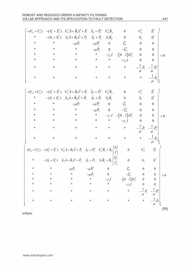
where 21V is a k k matrix. Finally, we get three LMIs for the reduced-order RFDF with order k as (59)

11 11 2 1 11 1 3 11 11 1

1 1 2 3 2 2 2 1

1 3

2

1 3

2

ˆ ˆ( ) ( ) 0ˆˆ ˆ ˆ* ( ) 0

ˆ ˆ* * 0 0 0ˆ ˆ* * * 0 0 0

* * * * 0 0 0* * * * * 0 0

1 1ˆ ˆ* * * * * *

1 ˆ* * * * * * *


T TF F d

T TF

TF

Td F

d

T



P P L

P LI I H

I

P P

P

0

11 11 2 1 11 1 3 11 11 1

1 1 2 3 2 2 2 1

1 3

2

1 3

2

ˆ ˆ( ) ( ) 0ˆˆ ˆ ˆ* ( ) 0

ˆ ˆ* * 0 0 0ˆ ˆ* * * 0 0 0

* * * * 0 0 0* * * * * 0 0

1 1ˆ ˆ* * * * * *

1 ˆ* * * * * * *


T TF F f

T TF

TF

Tf F

f

T



P P L

P LI I H

I

P P

P

0

11 11 2 1 11 1 3 11 11 1

1 1 2 3 2 2 2 1

1 3

2

0ˆ ˆ( ) ( ) 0

0ˆˆ ˆ ˆ ˆ* ( ) 0

ˆ ˆ* * 0 0 0ˆ ˆ* * * 0 0 0

* * * * 0 0 0* * * * * 0 0

1* * * * * *


T TF F u F

T TF

TF

Tu F

u



P P L

P LI I H

I

1 3

2

0

1ˆ ˆ

1 ˆ* * * * * * *

TP P

P

(59) where

www.intechopen.com


11 11 2 1 11 1 3 11 11 1

1 1 2 3 2 2 2 1

1 3

2

0ˆˆ ˆ ˆ ˆ( ) ( ) 0

0ˆˆ ˆ ˆ ˆ* ( ) 0

ˆ ˆ* * 0 0 0ˆ ˆ* * * 0 0 0

* * * * 0 0 0* * * * * 0 0

1 ˆ* * * * * *


T TF F u F

T TF

TF

Tu F

u



P P L

P LI I H

I

P

1 3

2

0

1 ˆ

1 ˆ* * * * * * *

TP

P

(56)

where

1 21 22 21T TS V V V , 2 21 22 12

T T TS V V V , 21ˆ TF FB V B , 1 1P̂ P , 1

2 21 22 2 22 21ˆ T TP V V PV V , 1

3 3 22 21ˆT TP P V V ,

121 22 21

ˆ TF FA V A V V , 1

22 21ˆF FL L V V and 1 3

3 2

ˆ ˆˆ

ˆ ˆ

TP PP

P P

.

To reduce the filter order, we’ll need partitions of the V and P variables as in (Kim & Watkins, 2007),

11 12

21 22

V VV

V V , 1 3

3 2

TP PP

P P (57)

Using the same method as in (Kim & Watkins, 2007), we can solve for the reduced-order filter whose filter order is ( )Fk k n . The partitioned sub-matrices in (57) will be dimensionalized as 11( ),F FV n n 12 ( ),FV n k 21( ),FV k n and 22 ( )V k k . We need to enforce some special structure on 21V as

21 21 ( )0Fk n kV V (58)

where 21V is a k k matrix. Finally, we get three LMIs for the reduced-order RFDF with order k as (59)

11 11 2 1 11 1 3 11 11 1

1 1 2 3 2 2 2 1

1 3

2

1 3

2

ˆ ˆ( ) ( ) 0ˆˆ ˆ ˆ* ( ) 0

ˆ ˆ* * 0 0 0ˆ ˆ* * * 0 0 0

* * * * 0 0 0* * * * * 0 0

1 1ˆ ˆ* * * * * *

1 ˆ* * * * * * *


T TF F d

T TF

TF

Td F

d

T



P P L

P LI I H

I

P P

P

0

11 11 2 1 11 1 3 11 11 1

1 1 2 3 2 2 2 1

1 3

2

1 3

2

ˆ ˆ( ) ( ) 0ˆˆ ˆ ˆ* ( ) 0

ˆ ˆ* * 0 0 0ˆ ˆ* * * 0 0 0

* * * * 0 0 0* * * * * 0 0

1 1ˆ ˆ* * * * * *

1 ˆ* * * * * * *


T TF F f

T TF

TF

Tf F

f

T



P P L

P LI I H

I

P P

P

0

11 11 2 1 11 1 3 11 11 1

1 1 2 3 2 2 2 1

1 3

2

0ˆ ˆ( ) ( ) 0

0ˆˆ ˆ ˆ ˆ* ( ) 0

ˆ ˆ* * 0 0 0ˆ ˆ* * * 0 0 0

* * * * 0 0 0* * * * * 0 0

1* * * * * *


T TF F u F

T TF

TF

Tu F

u



P P L

P LI I H

I

1 3

2

0

1ˆ ˆ

1 ˆ* * * * * * *

TP P

P

(59) where

www.intechopen.com

Fault Detection442

1 21 22 21T TS V V V , 1 1 ( )0

Fk n kS S , 2 21 22 12T T TS V V V , 21

ˆ TF FB V B ,

( )

ˆ

0F

FF

n k m

BB

, 1 1P̂ P ,

12 21 22 2 22 21ˆ T TP V V PV V , 1

3 3 22 21ˆT TP P V V , 1

21 22 21ˆ TF FA V A V V ,

( )

ˆ

0F

FF

n k k

AA

, 1

22 21ˆF FL L V V , and

1 3

3 2

ˆ ˆˆ

ˆ ˆ

TP PP

P P

.

Remark 4.2: The filter matrices ( , , )F F FA B L can be derived by the following procedure:

(i) Compute 22 21,V V by solving the factorization problem 1 21 22 21T TS V V V with the Schur

decomposition, (ii) Compute , ,F F FA B L : 1

21` 21 22ˆT

F FA V A V V 21

ˆTF FB V B , 1

21 22ˆ

F FL L V V █ Now, we need to remember that we had a polytopic uncertain system. As explained earlier,

the parameter dependent Lyapunov matrix ( )P , 1

( ) ( ),s

i ii

P P

is symmetric

positive definite for all admissible values of , if and only if, all the 'iP s are positive definite. Therefore, we need to check (59) only at the vertices, 1,2, ,i s . This gives us the final form (60)

11 11 2 1 11 1, 3, 11 , 11 1

1 1 2 3, 2, 2 , 2 1

1, 3,

2,

ˆ ˆ( ) ( ) 0ˆˆ ˆ ˆ* ( ) 0

ˆ ˆ* * 0 0 0ˆ ˆ* * * 0 0 0

* * * * 0 0 0* * * * * 0 0

1 ˆ* * * * * *

T T T T T T T Ti F i i F i d i

T Ti F i i F i d i

T Ti i F

Ti F

Td F

d



P P L

P LI I H

I

P

1, 3,

2,

0

1 ˆ

1 ˆ* * * * * * *

Ti i

i

P

P

11 11 2 1 11 1, 3, 11 , 11 1

1 1 2 3, 2, 2 , 2 1

1, 3,

2,

ˆ ˆ( ) ( ) 0ˆˆ ˆ ˆ* ( ) 0

ˆ ˆ* * 0 0 0ˆ ˆ* * * 0 0 0

* * * * 0 0 0* * * * * 0 0

1 ˆ* * * * * *

T T T T T T T Ti F i i F i f i

T Ti F i i F i f i

T Ti i F

Ti F

Tf F

f



P P L

P LI I H

I

P

1, 3,

2,

0

1 ˆ

1 ˆ* * * * * * *

Ti i

i

P

P

11 11 2 1 11 1, 3, 11 , 11 1

1 1 2 3, 2, 2 , 2 1

1, 3,

2,

0ˆ ˆ( ) ( ) 0

0ˆˆ ˆ ˆ ˆ* ( ) 0

ˆ ˆ* * 0 0 0ˆ ˆ* * * 0 0 0

* * * * 0

T T T T T T T Ti F i i F i u i F

T Ti F i i F i u i F

T Ti i F

Ti F

Tu F



P P L

P LI I H

1, 3,

2,

00 0

* * * * * 0 01 1ˆ ˆ* * * * * *

1 ˆ* * * * * * *

( 1,2, , )

u

Ti i

i

I

P P

P

i s

(60) Theorem 4.3: The reduced-order RFDF can be obtained by solving

11 1 2ˆ ˆ ˆ ˆ, , , , , , , , , ,

min : (60)F F F F d f u i

d d f f u uV S S A B L H P (61)

where ˆ 0P and , , and d f u are given as positive scalars. █ In summary, the reduced order RFDF filter in the multi-objective H formulation for polytopic uncertain system can be solved if and only if (60) holds for all vertices, 1,2, ,i s . The minimum value can be found from (61). Also, the filter realization ( , , , )F F F FA B L H defining the thk order filter is obtained from (i) and (ii) in Remark 4.2 and (61). Another important task for fault detection is the evaluation of the generated residual. An adaptive threshold will be used in this work. The disadvantage of a fixed threshold is that if we fix the threshold too low, it can increase the rate of false alarms. Thus, the optimal choice

www.intechopen.com


1 21 22 21T TS V V V , 1 1 ( )0

Fk n kS S , 2 21 22 12T T TS V V V , 21

ˆ TF FB V B ,

( )

ˆ

0F

FF

n k m

BB

, 1 1P̂ P ,

12 21 22 2 22 21ˆ T TP V V PV V , 1

3 3 22 21ˆT TP P V V , 1

21 22 21ˆ TF FA V A V V ,

( )

ˆ

0F

FF

n k k

AA

, 1

22 21ˆF FL L V V , and

1 3

3 2

ˆ ˆˆ

ˆ ˆ

TP PP

P P

.

Remark 4.2: The filter matrices ( , , )F F FA B L can be derived by the following procedure:

(i) Compute 22 21,V V by solving the factorization problem 1 21 22 21T TS V V V with the Schur

decomposition, (ii) Compute , ,F F FA B L : 1

21` 21 22ˆT

F FA V A V V 21

ˆTF FB V B , 1

21 22ˆ

F FL L V V █ Now, we need to remember that we had a polytopic uncertain system. As explained earlier,

the parameter dependent Lyapunov matrix ( )P , 1

( ) ( ),s

i ii

P P

is symmetric

positive definite for all admissible values of , if and only if, all the 'iP s are positive definite. Therefore, we need to check (59) only at the vertices, 1,2, ,i s . This gives us the final form (60)

11 11 2 1 11 1, 3, 11 , 11 1

1 1 2 3, 2, 2 , 2 1

1, 3,

2,

ˆ ˆ( ) ( ) 0ˆˆ ˆ ˆ* ( ) 0

ˆ ˆ* * 0 0 0ˆ ˆ* * * 0 0 0

* * * * 0 0 0* * * * * 0 0

1 ˆ* * * * * *

T T T T T T T Ti F i i F i d i

T Ti F i i F i d i

T Ti i F

Ti F

Td F

d



P P L

P LI I H

I

P

1, 3,

2,

0

1 ˆ

1 ˆ* * * * * * *

Ti i

i

P

P

11 11 2 1 11 1, 3, 11 , 11 1

1 1 2 3, 2, 2 , 2 1

1, 3,

2,

ˆ ˆ( ) ( ) 0ˆˆ ˆ ˆ* ( ) 0

ˆ ˆ* * 0 0 0ˆ ˆ* * * 0 0 0

* * * * 0 0 0* * * * * 0 0

1 ˆ* * * * * *

T T T T T T T Ti F i i F i f i

T Ti F i i F i f i

T Ti i F

Ti F

Tf F

f



P P L

P LI I H

I

P

1, 3,

2,

0

1 ˆ

1 ˆ* * * * * * *

Ti i

i

P

P

11 11 2 1 11 1, 3, 11 , 11 1

1 1 2 3, 2, 2 , 2 1

1, 3,

2,

0ˆ ˆ( ) ( ) 0

0ˆˆ ˆ ˆ ˆ* ( ) 0

ˆ ˆ* * 0 0 0ˆ ˆ* * * 0 0 0

* * * * 0

T T T T T T T Ti F i i F i u i F

T Ti F i i F i u i F

T Ti i F

Ti F

Tu F



P P L

P LI I H

1, 3,

2,

00 0

* * * * * 0 01 1ˆ ˆ* * * * * *

1 ˆ* * * * * * *

( 1,2, , )

u

Ti i

i

I

P P

P

i s

(60) Theorem 4.3: The reduced-order RFDF can be obtained by solving

11 1 2ˆ ˆ ˆ ˆ, , , , , , , , , ,

min : (60)F F F F d f u i

d d f f u uV S S A B L H P (61)

where ˆ 0P and , , and d f u are given as positive scalars. █ In summary, the reduced order RFDF filter in the multi-objective H formulation for polytopic uncertain system can be solved if and only if (60) holds for all vertices, 1,2, ,i s . The minimum value can be found from (61). Also, the filter realization ( , , , )F F F FA B L H defining the thk order filter is obtained from (i) and (ii) in Remark 4.2 and (61). Another important task for fault detection is the evaluation of the generated residual. An adaptive threshold will be used in this work. The disadvantage of a fixed threshold is that if we fix the threshold too low, it can increase the rate of false alarms. Thus, the optimal choice

www.intechopen.com

Fault Detection444

of the magnitude of the threshold depends upon the nature of the system uncertainties and varies with the system input. That is called an adaptive threshold. The first step of residual evaluation is to choose an evaluation function and to determine the corresponding threshold. Among a number of residual evaluation functions, the so-called time windowed root mean square (RMS) is often used. The time windowed RMS is represented as

,

1( ) ( ) ( )t

TRMS T

t T

r t r r dT

(62)

where T is the length of the finite time window. Since an evaluation of the residual signal over the whole time range is impractical, the time windowed RMS evaluation method is used in practice to detect faults as early as possible. After selecting the evaluation function, we are able to determine the threshold. A major requirement on the fault detection is to reduce or prevent false alarms. Thus, in the absence of any faults,

,( )

RMS Tr t should be less than the threshold value thJ , i.e.,

,, 0

sup ( )th RMS Tf

J r t

(63)

Under fault-free conditions, (63) can be described as

0 0( ) ( ) ( ) ( ) ( )ru rdr s T s u s T s d s (64) From Parseval’s Theorem (Zhou et al., 1996) and the RMS norm relationship (Boyd & Barratt, 1991), the threshold thJ can be found as follows

, , 0

0 0

,

0 0, ,

, ,

th RMS T f

ru rd RMS T

ru rdRMS T RMS T

u dRMS T RMS T

J r

T u T d

T u T d

u d

(65)

where u and d come from the optimization problem in (61) and

,RMS Td is calculated or

bounded by the worst disturbance acting on the plant. Thus in (65), ,RMS T

d is evaluated off-

line, while u(t) is assumed to be known and ,RMS T

u is calculated on-line.

5. Example

5.1 H Filter design In this example, we handle two cases, the full order and the reduced order filter design, and demonstrate the advantages of this study. We use the example from (Tuan et al., 2000) with the plant data

0 1 0.3 2 01 0.5 1 0

100 10 100 0 1

1 0

x x w

y x w

z x

(66)

where the uncertainty parameters, and , have four types of uncertainty sets given by

1, 1 (67)

1, (68)

3, 1 (69)

3, (70) Table 1 compares results between the filters in (Tuan, 2000, Geromel, 1999, De Souza, 1999) and (45) for the four types of uncertainties in (67)-(70). For the conservative case, a single Lyapunov matrix P is used and for the nonconservative case, four different Lyapunov matrices P are used for each vertex. The calculations were done using (Gahinet). An arbitrary positive scalar for should be chosen and the feasibility of the formulation should be checked. If it is feasible, the minimum value of (45) can be found.

Type Filter order

(Gero-mel, 1999):

2edT

(De Souza, 1999):

2edT

(Tuan, 2000): 2edT (45): edT

Non Conser- vative

Conser- vative

Non Conser- vative

Conser- vative

1, 1

full 5.728 4.867 2.382 5.7495 2.965 3.346 reduced 4.946 3.001 5.8467 3.179 4.304

1,

full 4.819 4.373 2.382 4.8841 2.948 3.165 reduced 4.556 3.079 5.0704 3.163 4.023

3, 1

full 93.365 + 29.106 + reduced 106.493 + 29.679 +

3,

full 100.963 + 28.808 + reduced 106.517 + 29.732 +

Table 1. Performance comparison according to each uncertainty type

www.intechopen.com


of the magnitude of the threshold depends upon the nature of the system uncertainties and varies with the system input. That is called an adaptive threshold. The first step of residual evaluation is to choose an evaluation function and to determine the corresponding threshold. Among a number of residual evaluation functions, the so-called time windowed root mean square (RMS) is often used. The time windowed RMS is represented as

,

1( ) ( ) ( )t

TRMS T

t T

r t r r dT

(62)

where T is the length of the finite time window. Since an evaluation of the residual signal over the whole time range is impractical, the time windowed RMS evaluation method is used in practice to detect faults as early as possible. After selecting the evaluation function, we are able to determine the threshold. A major requirement on the fault detection is to reduce or prevent false alarms. Thus, in the absence of any faults,

,( )

RMS Tr t should be less than the threshold value thJ , i.e.,

,, 0

sup ( )th RMS Tf

J r t

(63)

Under fault-free conditions, (63) can be described as

0 0( ) ( ) ( ) ( ) ( )ru rdr s T s u s T s d s (64) From Parseval’s Theorem (Zhou et al., 1996) and the RMS norm relationship (Boyd & Barratt, 1991), the threshold thJ can be found as follows

, , 0

0 0

,

0 0, ,

, ,

th RMS T f

ru rd RMS T

ru rdRMS T RMS T

u dRMS T RMS T

J r

T u T d

T u T d

u d

(65)

where u and d come from the optimization problem in (61) and

,RMS Td is calculated or

bounded by the worst disturbance acting on the plant. Thus in (65), ,RMS T

d is evaluated off-

line, while u(t) is assumed to be known and ,RMS T

u is calculated on-line.

5. Example

5.1 H Filter design In this example, we handle two cases, the full order and the reduced order filter design, and demonstrate the advantages of this study. We use the example from (Tuan et al., 2000) with the plant data

0 1 0.3 2 01 0.5 1 0

100 10 100 0 1

1 0

x x w

y x w

z x

(66)

where the uncertainty parameters, and , have four types of uncertainty sets given by

1, 1 (67)

1, (68)

3, 1 (69)

3, (70) Table 1 compares results between the filters in (Tuan, 2000, Geromel, 1999, De Souza, 1999) and (45) for the four types of uncertainties in (67)-(70). For the conservative case, a single Lyapunov matrix P is used and for the nonconservative case, four different Lyapunov matrices P are used for each vertex. The calculations were done using (Gahinet). An arbitrary positive scalar for should be chosen and the feasibility of the formulation should be checked. If it is feasible, the minimum value of (45) can be found.

Type Filter order

(Gero-mel, 1999):

2edT

(De Souza, 1999):

2edT

(Tuan, 2000): 2edT (45): edT

Non Conser- vative

Conser- vative

Non Conser- vative

Conser- vative

1, 1

full 5.728 4.867 2.382 5.7495 2.965 3.346 reduced 4.946 3.001 5.8467 3.179 4.304

1,

full 4.819 4.373 2.382 4.8841 2.948 3.165 reduced 4.556 3.079 5.0704 3.163 4.023

3, 1

full 93.365 + 29.106 + reduced 106.493 + 29.679 +

3,

full 100.963 + 28.808 + reduced 106.517 + 29.732 +

Table 1. Performance comparison according to each uncertainty type

www.intechopen.com

Fault Detection446

The feasibility must be checked because the product term of and Lyapunov variable P is nonlinear. We need to tune until the LMI solver returns a feasible solution. For any choice of 0 , if solvable, it gives a unique solution because of the convexity. For case (67), we found that when 7 (45) results in 2.965 for the full order case, and when 1.451 (45) results in 3.179 for the reduced order case. From Table 1, we can see that the optimization in (45) using parameter-dependent Lyapunov functions does not fail in the uncertainty cases of (69) and (70), but the conservative approaches in (De Souza, 1999, Gahinet) failed for the same cases. In the uncertainty cases of (69) and (70) cases, we also found that the conservative application of (Tuan et al., 2000) and our approach in (45), i.e., the usage of a single parameter-independent Lyapunov function, also failed. The filter data in the full and reduced order cases in (67) were found from (40)-(42). The Schur Decomposition method was used to solve the factorization problem in (40). The result is shown in Table 2 for the uncertainty case in (67).

Type Filter order FA FB FL

1, 1

full 23.5163 0.62426.3142 3.0403

0.00060.0031

588.5549 6.1988

reduced -0.8396 0.0022 4.0742

Table 2. Filter synthesis As we already know, the H approach in (45) is more robust to uncertainties than the 2H approach in (Tuan et al., 2000). To illustrate this, we found the filter data from (Tuan et al., 2000) and (45) and used (18) to calculate edT for the uncertainty case in (67). Table 3 shows the result. Therefore, we find that for this example our approach is more robust to model uncertainty than former approaches, (Tuan et al., 2000, Geromel, 1999, Gahinet) and gives a non-conservative result.

Type Filter order ( .,2000)Tuan et al (45)

3, 1 Full 11.1939 9.8752 Reduced 11.3486 10.7081

Table 3. Performance comparison between (Tuan et al., 2000) and (45)

5.2 Fault detection filter design In this section, a numerical example is given. Consider the uncertain LTI plant that is borrowed from (Nobrega et al., 2000), but is modified to include uncertainties. The plant is

0 1 0.3 1 0 0.11 0.5 1 1 0.2

100 10 100 0.1 0.05

x x u f d

y x u f d

(71)

where the uncertainty parameters, and , have the uncertainty set given by 1, 1 .

The selected reference model is 2( )2

W ss

. The fault signal f is simulated as a pulse of

unit amplitude that occurs from 20 to 25 seconds and is zero elsewhere. The input u is taken as 0.011 te . The unknown input d is assumed to be band-limited white noise with power 0.0005. The upper bound of

,RMS Td is given as 0.15. This value is used to calculate thJ of

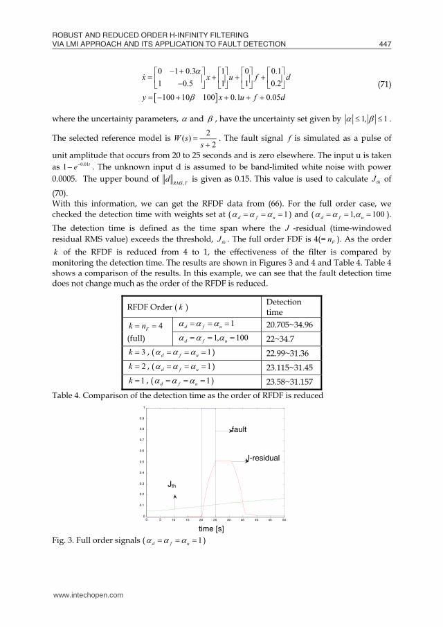
(70). With this information, we can get the RFDF data from (66). For the full order case, we checked the detection time with weights set at ( 1d f u ) and ( 1, 100d f u ). The detection time is defined as the time span where the J -residual (time-windowed residual RMS value) exceeds the threshold, thJ . The full order FDF is 4(= Fn ). As the order k of the RFDF is reduced from 4 to 1, the effectiveness of the filter is compared by monitoring the detection time. The results are shown in Figures 3 and 4 and Table 4. Table 4 shows a comparison of the results. In this example, we can see that the fault detection time does not change much as the order of the RFDF is reduced.

RFDF Order ( k ) Detection time

4Fk n (full)

1d f u 20.705~34.96 1, 100d f u 22~34.7

3k , ( 1d f u ) 22.99~31.36 2k , ( 1d f u ) 23.115~31.45 1k , ( 1d f u ) 23.58~31.157

Table 4. Comparison of the detection time as the order of RFDF is reduced

Fig. 3. Full order signals ( 1d f u )

0 5 10 15 20 25 30 35 40 45 500

0.1

0.2 0.3

0.4 0.5

0.6

0.7

0.8 0.9

1

time [s]

fault

J-residual

Jth

www.intechopen.com


The feasibility must be checked because the product term of and Lyapunov variable P is nonlinear. We need to tune until the LMI solver returns a feasible solution. For any choice of 0 , if solvable, it gives a unique solution because of the convexity. For case (67), we found that when 7 (45) results in 2.965 for the full order case, and when 1.451 (45) results in 3.179 for the reduced order case. From Table 1, we can see that the optimization in (45) using parameter-dependent Lyapunov functions does not fail in the uncertainty cases of (69) and (70), but the conservative approaches in (De Souza, 1999, Gahinet) failed for the same cases. In the uncertainty cases of (69) and (70) cases, we also found that the conservative application of (Tuan et al., 2000) and our approach in (45), i.e., the usage of a single parameter-independent Lyapunov function, also failed. The filter data in the full and reduced order cases in (67) were found from (40)-(42). The Schur Decomposition method was used to solve the factorization problem in (40). The result is shown in Table 2 for the uncertainty case in (67).

Type Filter order FA FB FL

1, 1

full 23.5163 0.62426.3142 3.0403

0.00060.0031

588.5549 6.1988

reduced -0.8396 0.0022 4.0742

Table 2. Filter synthesis As we already know, the H approach in (45) is more robust to uncertainties than the 2H approach in (Tuan et al., 2000). To illustrate this, we found the filter data from (Tuan et al., 2000) and (45) and used (18) to calculate edT for the uncertainty case in (67). Table 3 shows the result. Therefore, we find that for this example our approach is more robust to model uncertainty than former approaches, (Tuan et al., 2000, Geromel, 1999, Gahinet) and gives a non-conservative result.

Type Filter order ( .,2000)Tuan et al (45)

3, 1 Full 11.1939 9.8752 Reduced 11.3486 10.7081

Table 3. Performance comparison between (Tuan et al., 2000) and (45)

5.2 Fault detection filter design In this section, a numerical example is given. Consider the uncertain LTI plant that is borrowed from (Nobrega et al., 2000), but is modified to include uncertainties. The plant is

0 1 0.3 1 0 0.11 0.5 1 1 0.2

100 10 100 0.1 0.05

x x u f d

y x u f d

(71)

where the uncertainty parameters, and , have the uncertainty set given by 1, 1 .

The selected reference model is 2( )2

W ss

. The fault signal f is simulated as a pulse of

unit amplitude that occurs from 20 to 25 seconds and is zero elsewhere. The input u is taken as 0.011 te . The unknown input d is assumed to be band-limited white noise with power 0.0005. The upper bound of

,RMS Td is given as 0.15. This value is used to calculate thJ of

(70). With this information, we can get the RFDF data from (66). For the full order case, we checked the detection time with weights set at ( 1d f u ) and ( 1, 100d f u ). The detection time is defined as the time span where the J -residual (time-windowed residual RMS value) exceeds the threshold, thJ . The full order FDF is 4(= Fn ). As the order k of the RFDF is reduced from 4 to 1, the effectiveness of the filter is compared by monitoring the detection time. The results are shown in Figures 3 and 4 and Table 4. Table 4 shows a comparison of the results. In this example, we can see that the fault detection time does not change much as the order of the RFDF is reduced.

RFDF Order ( k ) Detection time

4Fk n (full)

1d f u 20.705~34.96 1, 100d f u 22~34.7

3k , ( 1d f u ) 22.99~31.36 2k , ( 1d f u ) 23.115~31.45 1k , ( 1d f u ) 23.58~31.157

Table 4. Comparison of the detection time as the order of RFDF is reduced

Fig. 3. Full order signals ( 1d f u )

0 5 10 15 20 25 30 35 40 45 500

0.1

0.2 0.3

0.4 0.5

0.6

0.7

0.8 0.9

1

time [s]

fault

J-residual

Jth

www.intechopen.com

Fault Detection448

Fig. 4. Reduced order ( 1k ) signals ( 1d f u )

6. Conclusion

In this paper, we developed in detail a practical approach for solving the H reduced filter synthesis problem in an LMI framework and its application for fault detection filter design. The LMI characteristics of the filtering problem were described and formulated with the BRL. To overcome conservatism, parameter-dependent Lyapunov functions were used. A congruence transformation and a change of variable technique were used to linearize the problem. This formulation had formerly been applied to the 2H problem. As is well-known, the H approach provides better robustness than the 2H approach. The order reduction problem for a robust fault detection filter was considered, and the result was illustrated with a simple example. A reference model was introduced and formulated as a multi-objective optimization for a polytopic uncertain system. The order of the RFDF is reduced using LMI techniques and the detection performance is compared with the full order filter. Using the LMI solver from Mathworks Robust Control Toolbox, the minimum value is found from (61). For the example considered, the detection time did not change much as the filter order was reduced. Thus, our reduced-order RFDF design shows promising results.

7. References

Bettayeb, M. & Kavranoglu, D. (1994). Reduced order H filtering, Proceedings of American Control Conference, pp. 1884-1888

Boyd, S. & Barratt, C. (1991). Linear Controller Design, Limits of Performance, Prentice Hall, pp. 98-99

Casavola, A.; Famularo, D. & Franze, G. (2003). Robust fault isolation of uncertain linear systems: An LMI approach, Proceedings of the IFAC Fault Detection Supervision and Safety of Technical Processes

Casavola, A.; Famularo, D. & Franze, G. (2005a). A robust deconvolution scheme for fault detection and isolation of uncertain linear systems: an LMI approach, Automatica, 41, pp. 1463-1472

0 5 10 15 20 25 30 35 40 45 50 0

0.1

0.2

0.3

0.4

0.5

0.6

0.7

0.8

0.9

1

time [s]

fault

J-residual Jth

Casavola, A.; Famularo, D.; & Franze, G. (2005b). Robust fault detection of uncertain linear systems via quasi-LMIs, Proceedings of American Control Conference, pp. 1654-1659

Chen, J. & Zhang, H. Y. (1991). Robust detection of faulty actuators via unknown input observers, International Journal of Systems Science, Vol. 22, No. 10, pp. 1829-1839

Chen, J. & Patton, R. J. (1997). Observer-based fault detection and isolation: robustness and applications, Control Engineering Practice, Vol. 5, No. 5, pp. 671-682

Chen, J. & Patton, R. J. (1999). Robust Model-Based Fault Diagnosis for Dynamic Systems, Kluwer Academic Publishers

De Souza, C. E. & Trofino, A. (1999). An LMI approach to the design of robust 2H filters, Recent Advances in Linear Matrix Inequality Methods in Control, SIAM, Philadelphia, PA

Ding, S. X.; Frank, P. M.; Ding, E. L. & Jeinsch, T. (2000). Fault detection system design based on a new trade-off strategy, Proceedings of 39th IEEE Conference on Decision and Control, pp. 4144-4149

Ding, S. X. & Frank, P. M. (2003). Threshold calculation using LMI- technique and its integration in the design of fault detection systems, Proceedings of 42nd IEEE Conference on Decision and Control, pp. 469-474

Frisk, E. (2001). Residual Generation for Fault Diagnosis, Ph.D. dissertation, Dept. of Electrical Engineering, Linkoping University, Sweden

Fu, M.; De Souza, C. E. & Xie, L. (1994). H estimation for uncertain systems, International Journal of Robust and Nonlinear Control, Vol. 4, pp. 421-448

Gahinet, P. & Apkarian, P. (1994). A linear matrix inequality approach to H control, International Journal of Robust and Nonlinear Control, Vol. 4, pp. 421-448

Gahinet, P.; Apkarian, P. & Chilali, M. (1996). Parameter dependent Lyapunov functions for real parametric uncertainty, IEEE Transactions on Automatic Control, Vol. 41, pp. 436-442

Gahinet, P.; Nemirovski, A.; Laub, A. J. & Chilali, M. The LMI Control Toolbox Tutorial, MATLAB v7.0, Mathworks Inc.

Geromel, J. C. (1999). Optimal linear filtering under parameter uncertainty, IEEE Transactions on Signal Processing, Vol. 47, pp. 168-175

Grigoriadis, K. M. & Watson, J. T. (1997). Reduced order H and 2L L filtering via linear matrix Inequalities, IEEE Transactions on Aerospace and Electronic Systems, Vol. 33, pp. 1326-1338

Kim, Y-M. & Watkins, J. M. (2006). A New Approach for Robust and Reduced Order H Filtering, Proceedings of American Control Conference, pp. 5171-5176, Minneapolis, MN

Kim, Y-M. & Watkins, J. M. (2007). A new approach for robust and reduced order fault detection filter design, Proceedings of American Control Conference, New York, NY

Nagpal, K. M.; Helmick, R. E. & Sims, C. S. (1987). Reduced order estimation, I. Filtering, International Journal of Control, Vol. 45, pp. 1867-1888

Niemann, H. & Stoustrup, J. (2000). Design of fault detectors using H optimization, Proceedings of the 39th IEEE Conference on Decision and Control, pp. 4327-4328

Nobrega, E. G. & Abdalla, M. O. (2000). Grigoriadis, K. M.; LMI-based filter design for fault detection and isolation, Proceedings of 39th IEEE Conference on Decision and Control, pp. 4329-4334

www.intechopen.com


Fig. 4. Reduced order ( 1k ) signals ( 1d f u )

6. Conclusion

In this paper, we developed in detail a practical approach for solving the H reduced filter synthesis problem in an LMI framework and its application for fault detection filter design. The LMI characteristics of the filtering problem were described and formulated with the BRL. To overcome conservatism, parameter-dependent Lyapunov functions were used. A congruence transformation and a change of variable technique were used to linearize the problem. This formulation had formerly been applied to the 2H problem. As is well-known, the H approach provides better robustness than the 2H approach. The order reduction problem for a robust fault detection filter was considered, and the result was illustrated with a simple example. A reference model was introduced and formulated as a multi-objective optimization for a polytopic uncertain system. The order of the RFDF is reduced using LMI techniques and the detection performance is compared with the full order filter. Using the LMI solver from Mathworks Robust Control Toolbox, the minimum value is found from (61). For the example considered, the detection time did not change much as the filter order was reduced. Thus, our reduced-order RFDF design shows promising results.

7. References

Bettayeb, M. & Kavranoglu, D. (1994). Reduced order H filtering, Proceedings of American Control Conference, pp. 1884-1888

Boyd, S. & Barratt, C. (1991). Linear Controller Design, Limits of Performance, Prentice Hall, pp. 98-99

Casavola, A.; Famularo, D. & Franze, G. (2003). Robust fault isolation of uncertain linear systems: An LMI approach, Proceedings of the IFAC Fault Detection Supervision and Safety of Technical Processes

Casavola, A.; Famularo, D. & Franze, G. (2005a). A robust deconvolution scheme for fault detection and isolation of uncertain linear systems: an LMI approach, Automatica, 41, pp. 1463-1472

0 5 10 15 20 25 30 35 40 45 50 0

0.1

0.2

0.3

0.4

0.5

0.6

0.7

0.8

0.9

1

time [s]

fault

J-residual Jth

Casavola, A.; Famularo, D.; & Franze, G. (2005b). Robust fault detection of uncertain linear systems via quasi-LMIs, Proceedings of American Control Conference, pp. 1654-1659

Chen, J. & Zhang, H. Y. (1991). Robust detection of faulty actuators via unknown input observers, International Journal of Systems Science, Vol. 22, No. 10, pp. 1829-1839

Chen, J. & Patton, R. J. (1997). Observer-based fault detection and isolation: robustness and applications, Control Engineering Practice, Vol. 5, No. 5, pp. 671-682

Chen, J. & Patton, R. J. (1999). Robust Model-Based Fault Diagnosis for Dynamic Systems, Kluwer Academic Publishers

De Souza, C. E. & Trofino, A. (1999). An LMI approach to the design of robust 2H filters, Recent Advances in Linear Matrix Inequality Methods in Control, SIAM, Philadelphia, PA

Ding, S. X.; Frank, P. M.; Ding, E. L. & Jeinsch, T. (2000). Fault detection system design based on a new trade-off strategy, Proceedings of 39th IEEE Conference on Decision and Control, pp. 4144-4149

Ding, S. X. & Frank, P. M. (2003). Threshold calculation using LMI- technique and its integration in the design of fault detection systems, Proceedings of 42nd IEEE Conference on Decision and Control, pp. 469-474

Frisk, E. (2001). Residual Generation for Fault Diagnosis, Ph.D. dissertation, Dept. of Electrical Engineering, Linkoping University, Sweden

Fu, M.; De Souza, C. E. & Xie, L. (1994). H estimation for uncertain systems, International Journal of Robust and Nonlinear Control, Vol. 4, pp. 421-448

Gahinet, P. & Apkarian, P. (1994). A linear matrix inequality approach to H control, International Journal of Robust and Nonlinear Control, Vol. 4, pp. 421-448

Gahinet, P.; Apkarian, P. & Chilali, M. (1996). Parameter dependent Lyapunov functions for real parametric uncertainty, IEEE Transactions on Automatic Control, Vol. 41, pp. 436-442

Gahinet, P.; Nemirovski, A.; Laub, A. J. & Chilali, M. The LMI Control Toolbox Tutorial, MATLAB v7.0, Mathworks Inc.

Geromel, J. C. (1999). Optimal linear filtering under parameter uncertainty, IEEE Transactions on Signal Processing, Vol. 47, pp. 168-175

Grigoriadis, K. M. & Watson, J. T. (1997). Reduced order H and 2L L filtering via linear matrix Inequalities, IEEE Transactions on Aerospace and Electronic Systems, Vol. 33, pp. 1326-1338

Kim, Y-M. & Watkins, J. M. (2006). A New Approach for Robust and Reduced Order H Filtering, Proceedings of American Control Conference, pp. 5171-5176, Minneapolis, MN

Kim, Y-M. & Watkins, J. M. (2007). A new approach for robust and reduced order fault detection filter design, Proceedings of American Control Conference, New York, NY

Nagpal, K. M.; Helmick, R. E. & Sims, C. S. (1987). Reduced order estimation, I. Filtering, International Journal of Control, Vol. 45, pp. 1867-1888

Niemann, H. & Stoustrup, J. (2000). Design of fault detectors using H optimization, Proceedings of the 39th IEEE Conference on Decision and Control, pp. 4327-4328

Nobrega, E. G. & Abdalla, M. O. (2000). Grigoriadis, K. M.; LMI-based filter design for fault detection and isolation, Proceedings of 39th IEEE Conference on Decision and Control, pp. 4329-4334

www.intechopen.com

Fault Detection450

O’Brien Jr., R. T. & Kiriakidis, K. (2004). Reduced-order H filtering for discrete time linear time varying systems, Proceedings of American Control Conference, pp. 4120-4125

Patton, R. J. & Hou, M. (1999). On sensitivity of robust fault detection observers, 14th IFAC World Congress, pp. 67-72

Tuan, H. D.; Apkarian, P. & Nguyen, T. Q. (2000). Robust and reduced order filtering: New characterizations and methods, Proceedings of American Control Conference, pp. 1327-1331

Zhong, M.; Ding, S. X.; Lam, J. & Wang, H. (2003). An LMI approach to design robust fault detection filter for uncertain LTI systems, Automatica, 39, pp. 543-550

Zhou, K.; Doyle, J. C. & Glover, K. (1996). Robust and Optimal Control, Prentice Hall

www.intechopen.com

Fault DetectionEdited by Wei Zhang

ISBN 978-953-307-037-7Hard cover, 504 pagesPublisher InTechPublished online 01, March, 2010Published in print edition March, 2010

InTech EuropeUniversity Campus STeP Ri Slavka Krautzeka 83/A 51000 Rijeka, Croatia Phone: +385 (51) 770 447 Fax: +385 (51) 686 166www.intechopen.com

InTech ChinaUnit 405, Office Block, Hotel Equatorial Shanghai No.65, Yan An Road (West), Shanghai, 200040, China

Phone: +86-21-62489820 Fax: +86-21-62489821

In this book, a number of innovative fault diagnosis algorithms in recently years are introduced. Thesemethods can detect failures of various types of system effectively, and with a relatively high significance.

How to referenceIn order to correctly reference this scholarly work, feel free to copy and paste the following:

Young-Man Kim and John M. Watkins (2010). Robust and Reduced Order H-Infinity Filtering via LMI Approachand Its Application to Fault Detection, Fault Detection, Wei Zhang (Ed.), ISBN: 978-953-307-037-7, InTech,Available from: http://www.intechopen.com/books/fault-detection/robust-and-reduced-order-h-infinity-filtering-via-lmi-approach-and-its-application-to-fault-detectio

© 2010 The Author(s). Licensee IntechOpen. This chapter is distributedunder the terms of the Creative Commons Attribution-NonCommercial-ShareAlike-3.0 License, which permits use, distribution and reproduction fornon-commercial purposes, provided the original is properly cited andderivative works building on this content are distributed under the samelicense.

https://creativecommons.org/licenses/by-nc-sa/3.0/

H-INFINITY FILTERING VIA LMI APPROACH AND ITS APPLICATION

Documents

Transcript of H-INFINITY FILTERING VIA LMI APPROACH AND ITS APPLICATION