Naval Research LaboratoryWashington, DC 20375-5320

AD-A277 2891 NRL/MR/6707--94-7444

Gyrotrons and Free Electron Lasersfor Atmospheric Sensing

WALLACE M. MANHEIMER

DTICSenior Scientist Fundamental Plasma Processes EL E CT V*Plasma Physics Division MAR24 19943 F

F U

February 28, 1994

94-09203hll II l ll l 111111

Aroved for public release; distribution unlimited.

94 3 23 0

REPORT DOCUMENTATION PAGE FmAWOW8 ft. 070-01 as

1Pe ,esmoo eiw bdw foe* ealsee eE Wwmwen ma esmed to w-qp I haw mpoe. dewd•dfi ido la* foruoww weeni . rnw inis do" ewuam

laOWq "! iWe i. dot needwedi.. e0e1d &lW ies b hn eulsbi e4 dU•waIwlm eard ewawe m din edem ,. ot aiw so m d o

edesdeni t @1 b iemt sle i et m fw I g msw bwdetoWidiWWren11 N ed rSe imeete hwm O e i a , 1215len~Dovio iWas, buie 1204. Au %en. VA 222024302. aide ohO Offi0 eo MIe i d & udget. Pow wk RedtIdum Peget 0704.o0100. Wedaiqms DC 20603.

1. AGENCY USE ONLY .a~vw Msnk) 2. REPORT DATE 3. REPORT TYPE AND DATES COVERED

February 28, 1994 Interim4. TITLE AND SUBTITLE S. FUNDING NUMBERS

Gyrotrons and Free Electron Lasers for Atmospheric Sensing PE - 61153N

6. AUTHOR(S)

W. M. Manheimer

7. PERFORMING ORGANIZATION NAME(S) AND ADOOSSIES) B. PERFORMING ORGANIZATIONREPORT NUMBER

Naval Research LaboratoryWashington, DC 20375-5320 NRL/MR/6707-94-7444

9. SPONSORING/MONITORING AGENCY NAME(S) AND ADORESSIES) 10. SPONSORING/MONITORINGAGENCY REPORT NUMBER

Office of Naval Pasearch800 N Quincy StredArlington, VA 22217-5660

11. SUPPLEMENTARY NOTES

12a. DISTRUJTIONIAVAILABILITY STATEMENT 12b. DISTRIBUTION CODE

Approved for public release; distribution unlimited.

13. ABSTRACT (AMxdwmm 200 Wtoi)

The development of gyrotrons and free electron lasers over the past decade and a half have naturally led to investigations ofadditional applications for them. This work looks into applications in the area of atmospheric sensing. Specific gyrotron applicationsinclude cloud radars, sensors for atmospheric turbulence, and measurement schemes for upper atmosphere race impurities. To beuseful as atmospehric sensors, fiee electon lasers must be made much more compact. Several development strategies foraccomplishing this are possible. It appears that there are numerous potential applications for both gyrotrons and free electron lasersas atmospheric sensors.

14. SUBJECT TERMS 16. NUMBER OF PAGES

Gyrotrons 69Free electron lasers 16. PRcE CODEAtmospheric sensing

17. SECURITY CLASSIFICATION IS. SECURITY CLASSIFICATION 19. SECURITY CLASSIFICATION 20. LIMITATION OF ABSTRACTOF REPORT OF THIS PAGE OF ABSTRACT

UNCLASSIFIED UNCLASSIFIED UNCLASSIFIED UL

N 7540.01-2110-600 Skadad r.,m 29t8 ORev. 24-)ftr-be0 by ANN Nd 2W16

i ~2MI-02

CONTENTS

I. INTRODUCTION ................................................ 1

U. GYROTRONS, FREE ELECTRON LASERS AND ATMOSPHERIC PROPAGATION .... 2

MI. CLOUD RADAR STUDIES WITH HIGH POWER GYROTRONS ................ 10

IV. REMOTE SENSING OF ATMOSPHERIC TURBULENCE ..................... 18

V. REMOTE SENSING OF TRACE IMPURITIES IN THE UPPER ATMOSPHERE ...... 22

VI. ATMOSPHERIC SENSING WITH FREE ELECTRON LASERS ................. 31

VII. CONCLUSION ................................................... 33

ACKNOWLEDGEMENT .......................................... 34

REFERENCES ................................................. 35

lllii

GYROTRONS AND FREE ELECTRON LASERSSFOR ATMOSPHERIC SENSING

I. Introduction

Gyrotrons have been developed over the last decade and a halfor so for, and to a large extent, by plasma physicists. Free electronlasers (FEL's) were also developed in part by plasma physicists.Gyrotrons have been developed mostly for heating of fusion plasmas,and free electron lasers, as a powerful source of infrared (IR)radiation where none have previously existed. Both of them aregenerally thought of being situated in large, fixed facilities. In fact,FEL's often are the fixed facility, as they require a high energyelectron accelerator and a heavily shielded enclosure. Howevergyrotrons are compact enough that they could be fielded in forinstance a small truck. While IRFEL's cannot currently be fielded,there are several possible development strategies which could leadto a fieldable source in the not too distant future.

The field of atmospheric sensing has benefited enormouslyover recent decades from the use of radar and laser probes. Radarsare generally at low frequency, typically X-Band or below, andtunable lasers are usually optical or shorter wavelength. (Fixedfrequency or line tunable lasers are available at a few wavelengthsin the infrared.) The development of fixed frequency gyrotronsopens up the possibility of cloud radars. Millimeter wave radiationat 94 GHz has the unique capability of scattering weakly from cloudaerosol droplets, which really define the cloud, while at the sametime propagating easily through the cloud. It could for instancesense multiple cloud layers, whereas a lidar would be stopped by thefirst cloud not visibly transparent. Tunable gyrotrons open up newpossibilities of absorption measurements over long path lengths.Detection of trace elements at sea level and in the upper atmosphereis also possible. Furthermore, high power gyrotrons, in bistatic radarconfigurations, open up additional possibilities for remote sensing ofclear air turbulence. Tunable, powerful, infrared free electron laserscould allow for the detection of new classes of atmosphericimpurities by using them as differential absorption lidars at muchgreater range.

Manuwipt approved January 13, 1994.

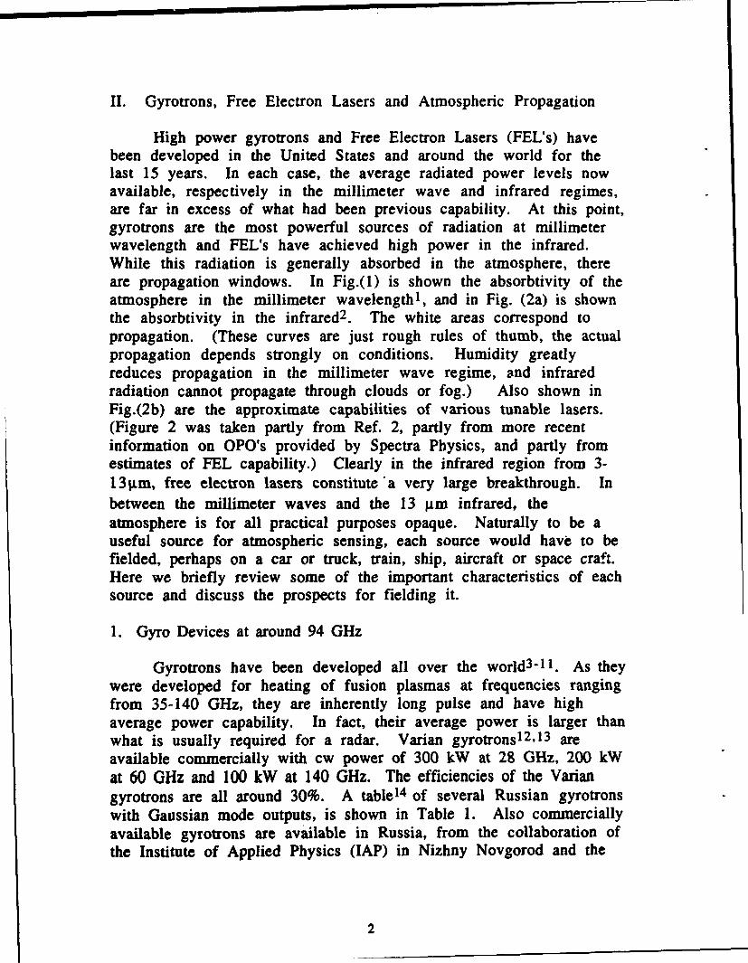
II. Gyrotrons, Free Electron Lasers and Atmospheric Propagation

High power gyrotrons and Free Electron Lasers (FEL's) havebeen developed in the United States and around the world for thelast 15 years. In each case, the average radiated power levels nowavailable, respectively in the millimeter wave and infrared regimes,are far in excess of what had been previous capability. At this point,gyrotrons are the most powerful sources of radiation at millimeterwavelength and FEL's have achieved high power in the infrared.While this radiation is generally absorbed in the atmosphere, thereare propagation windows. In Fig.(1) is shown the absorbtivity of theatmosphere in the millimeter wavelength1 , and in Fig. (2a) is shownthe absorbtivity in the infrared 2 . The white areas correspond topropagation. (These curves are just rough rules of thumb, the actualpropagation depends strongly on conditions. Humidity greatlyreduces propagation in the millimeter wave regime, and infraredradiation cannot propagate through clouds or fog.) Also shown inFig.(2b) are the approximate capabilities of various tunable lasers.(Figure 2 was taken partly from Ref. 2, partly from more recentinformation on OPO's provided by Spectra Physics, and partly fromestimates of FEL capability.) Clearly in the infrared region from 3-13gm, free electron lasers constitute *a very large breakthrough. Inbetween the millimeter waves and the 13 gm infrared, theatmosphere is for all practical purposes opaque. Naturally to be auseful source for atmospheric sensing, each source would have to befielded, perhaps on a car or truck, train, ship, aircraft or space craft.Here we briefly review some of the important characteristics of eachsource and discuss the prospects for fielding it.

1. Gyro Devices at around 94 GHz

Gyrotrons have been developed all over the world 3-11. As theywere developed for heating of fusion plasmas at frequencies rangingfrom 35-140 GHz, they are inherently long pulse and have highaverage power capability. In fact, their average power is larger thanwhat is usually required for a radar. Varian gyrotrons1 2,13 areavailable commercially with cw power of 300 kW at 28 GHz, 200 kWat 60 GHz and 100 kW at 140 GHz. The efficiencies of the Variangyrotrons are all around 30%. A table 14 of several Russian gyrotronswith Gaussian mode outputs, is shown in Table 1. Also commerciallyavailable gyrotrons are available in Russia, from the collaboration ofthe Institute of Applied Physics (IAP) in Nizhny Novgorod and the

2

Tory Company in Moscow. One available there, which we willmention shortly is the 83 GHz cw gyrotron at a power of 10 kW. Amillimeter wave radar with these peak sorts of peak powers, and aduty factor of 0.1-10%, constitutes a breakthrough in millimeterwave radar power by several orders of magnitude. However it isfairly modest as regards gyrotron capability.

One of the few gyrotrons designed at a frequency optimized foratmospheric propagation is the NRL 94 GHz gyrotron15 ,16 . This hasgenerated up to 200 kW of power at 94 GHz with efficiencies ofabout 20%. This frequency is the clearest part of the atmosphericpropagation window. Also tunable gyrotrons have been developed atNRL. 11

The development of powerful gyro amplifiers at frequenciesnear 94 GHz is also proceeding. For many radar applications, anamplifier is preferable to a free running oscillator. This allows phaseand amplitude control of the transmitted beam. If an amplifier andan oscillator are both available, and all other things are equal, theamplifier is the preferred rf source to power a radar. For one thing,data processing is simpler if the amplitude and phase are preciselyknown pulse to pulse. Nevertheless the data processing can be donewith an oscillator transmitter. Also, it may be necessary tocoherently combine power from one or more sources. This can onlybe done with totally coherent signals produced by an amplifier.Counterbalancing the advantages of amplifiers are the fact that theyare more complicated and expensive than oscillators, due to thenecessity of having the additional microwave plumbing for the inputsignal. Also there are more stringent requirements of avoiding bothoscillation and intercavity cross talk anywhere in the amplifier,which is usually longer than an oscillator. For an atmospheric sensorapplication, the choice of an oscillator or amplifier will be made interms of requirements as well as price and availability of whateverthe source would be.

At this point the most advanced is a gyroklystron developed atthe Institute of Applied Physics (IAP) in Nizhny Novgorod in Russia17

which has generated power in excess of 50 kW at 94 GHz. The NRLquasi-optical gyrotron, when run in a gyroklystron configuration hasalso demonstrated capability as- both an amplifier and a phase lockedoscillator1 8 ,19 . The basic difference is that the IAP gyroklystron usesrelatively low Q cavities so that its bandwidth is relatively high,some fraction of a percent. The quasi-optical gyroklystron uses a

23

much higher Q cavity, so its bandwidth is much les§. The two arecomplementary in that the former could find application wherebandwidth is required; the latter where great frequency and phasestability is required.

All gyro devices at 94 GHz use super conducting magnets,although future developments of high harmonic gyrotrons mightrender these unnecessary 2 0 . However if one can live with theconstraints of a super conducting magnet, any of these gyrotrons arereasonably compact, certainly compact enough to be transported on asmall truck or multi-engine aircraft. Thus they could be fielded asradars. We now discuss the sources in somewhat more detail.

A. The NRL 94 GHz Gyrotron

The 94 GHz gyrotron is a TE1 3 mode gyrotron which hasgenerated 150 kW of power in a lIs pulse at an efficiency of 15-20%.With appropriate cooling on the collector and window, it couldoperate at an average power of 10 kW. This is in fact only 10% ofthe average power Varian has demonstrated in their 140 GHzgyrotron. Another advantage to the mnode selected is that it can befairly easily converted to a fundamental TEIl mode for propagation.A mode converter has been developed by General Atomics, SanDiego, Cal, and is currently in place on our gyrotron. Conversion tothe TEll mode has been demonstrated. The measured far field modepattern of the NRL 94 GHz gyrotron in Fig.(3) shows that the outputis in fundamental mode.

Figure 4 is a schematic of the gyrotron with the modeconverter in place, Fig 5 is a photograph of the gyrotron laboratory.Figure 2 shows the two stage mode converter (TE13-+TE12 followedby TE21-+TEII). The equipment is compact and can easily betransported on a small truck. This capability to radiate averagepowers of order 10 KW at 94 GHz into the atmosphere represents avery new capability.

Another important figure of merit for the gyrotron oscillator isbandwidth, which directly translates to range resolution in a radar.Since the Q of the NRL gyrotron is 600, this corresponds to arelatively wide bandwidth. The gyrotron can be tuned by varyingthe voltage during a pulse. Shown in Fig.(6) is a plot of the

4

frequency variation of the NRL 94 GHz gyrotron, generated by a timedependent simulation, where the voltage increased from 60 to 70 kVin about 20 nsec (the time chosen for numerical convenience). Herethe chirp is about 200 MHz, corresponding to a range resolution ofabout a meter for optimal data processing in the receiver circuit.Operation of the NRL 94 GHz gyrotron at different voltages havebasically confirmed this calculation.

B. The Tunable NRL Quasi-Optical Gyrotron

The quasi-optical gyrotron is a very different sort of a gyrotronin an optical resonator. It has been developed at both NRL2 1-24 andLausanne 2 5 . The beam propagation and the magnetic field are bothtransverse to the axis of the resonator. The mode output is taken bydiffraction around the mirror. The diffraction is characterized by afractional loss v per round trip of the radiation. Typically the NRLexperiment runs with v's between 1 and 5%. In theory and in fact,the resonator operates only in the lowest order fundamentaltransverse mode.

Figure 7 is a photograph of the quasi-optical gyrotron. It isabout as portable as the conventional gyrotron. The maximumpower it has achieved so far is 600 kW, but at relatively low 8%efficiency. More recent experiments, at the 100 kW power levelhave used a number of schemes to increase the efficiency. Themaximum efficiency achieved so far is about 20% without adepressed collector and 30% with one18 ,19 . While the efficiency ofthe quasi-optical gyrotron is typically lower than that of a cavitygyrotron, this is largely counterbalanced by the fact that because ofits cross bore geometry, a single stage depressed collector isparticularly simple to implement.

One of the most attractive features of the quasi-opticalgyrotron is its tunability. It can be tuned in three ways: * Themagnetic field can be varied over a fairly wide range. The power isrelatively insensitive to field. Figure 8a shows a plot of modefrequency and power as a function of magnetic field for a series oflower power experiments. The device can tune over about half anoctave from about 80 to 130 GHz. * The device can be tuned with

the beam voltage. Since the frequency scales as B/y, the frequencycan be raised by lowering the voltage. Figure 8b shows the Voltagetuning curve. Clearly the power is now sensitive to voltage if only

5

because the input power is proportional to it. However this voltagedependence does allow rapid tuning over a small frequency rangeThe cavity can be tuned by adjusting the mirror separation, whichcan be done without breaking vacuum. This allows for very precisetuning.

It is also possible that the quasi-optical gyrotron could operateat the second harmonic. The Lausanne experiment has already seenevidence of harmonic operation. If it can run with harmonicoperation, it opens the possibility of a single source covering theentire spectral region from 80 to 260 GHz.

C. The IAP 94 GHz Gyroklystron

The IAP amplifier development program is the most mature atthis point 17 . It has developed powerful tubes at 35 and 94 GHzwhich have been reported only recently. A 94 GHz gyroklystron hasbeen developed at lAP and is a four cavity interaction circuit. Thecavities are all in the TE0 1 mode. Shown in Fig.(9) is a schematic ofthe interaction circuit superimposed on the background magneticfield. At the peak, the field is 37 kG. In Fig. (10) is shown a plot ofits power, gain and bandwidth. In this case the achieved power is 60kW and the bandwidth is about 400 MHz. For the data shown here,the efficiency was somewhat over 30%. While the IAP program hasbeen in existence for a long time and is quite mature, only recentlyhas information on it been available.

D. The NRL Gyroklystron Amplifier

This configuration uses a Fabre Perot resonator with both theelectron beam and magnet field direction perpendicular to the axis ofthe resonator. Just upstream from the main resonator is a small,lower Q prebunching resonator. At the currents and perpendicularvelocities of the beam, this upstream resonator is always below startoscillation threshold 1 8,19 . The experiment was done at 85 GHzbecause that was the frequency of the available drive source. It wasan extended interaction oscillator (E0O) which put out a power of 1kW for a 2 jis pulse. Power from the EIO was fed into the upstreamresonator, it prebunched the beam, and the amplified power wasextracted at the main resonator. A schematic of the quasi-opticalgyroklystron is shown in Fig.(l 1).

6

Since the main resonator had a very high Q, the bandwidth wasvery low, about 3 MHz, which is about equal to co/Q. A plot ofamplification as a function of cathode voltage, as compared with anumerical simulation is shown in Fig.(12). In this series ofexperiments, the power is about 30 kW and the efficiency is about10%. By increasing the current somewhat, one can exceed the startcurrent in the main cavity, but remain below it in the prebunchingcavity. In this case one can drive a phase locked oscillator. Here theoscillator is no longer free running, but has its phase controlled bythe much weaker input signal. This is an alternate realization of aphase controlled source. When run as a phase locked oscillator, thedevice had a power of 60 kW and an efficiency of 16%. In Fig.(13) isshown the phase locking bandwidth as a function of input to outputpower ratio. The curve is Adler's classic theory2 6 for the case ofphase locking by direct injection of power into the output port of thedevice. This is

UfL = (fo/2Q)[Pi/Po]I/2

where 8fL is the locking bandwidth and Pi/Po is the injection/outputpower. Clearly the prebunching allows one to greatly exceed theAdler theory. Also because power is injected into a prebunchingcavity and not the output, there is no need for a high powermillimeter wave circulator.

The quasi-optical gyroklystron is inherently a much narrowerband than the conventional cavity configuration. Thus it would findits application where great frequency stability is the most importantcharacteristic. An example night be a radar whose main role is to doDoppler sorting of a large number of low cross section targets withslightly different velocities. Also it does have additional advantagesdue to its simplicity, intercavity isolation, and adaptability. None ofthe cavities has any inherent frequency other than c/Lm where Lm isthe mirror separation, so it will have a very large inherent tuningrange. The cavities are naturally isolated from one another, and atno point during the experiment was there ever any evidence of crosstalk. Furthermore, while the cavity Q was very high, this too isflexible and can be lowered by moving the mirrors closer togetherand, by changing the radius of the mirror edge so as to vary theoutput coupling. Thus the bandwidth and the power can beincreased with straightforward scaling.

7

2 Infrared Free Electron Lasers

Free electron lasers are currently large facilities which take upan entire building, often a very large one. As currently configured,they cannot be fielded. There are two reasons the facilities are solarge. First of all, they require a multi megavolt electron beam; andsecond, because of this beam, they need a tremendous amount ofradiation shielding. Thus there are two requirements to field an FEL.First one must reduce the beam energy as much as possible; andsecond, one must recover as much of the beam energy as possiblewith the use of a depressed collector. There seem to be two FELconfigurations which could potentially evolve toward a device whichcan be fielded.

The first is the electrostatic accelerator use in the University ofCalifornia at Santa Barbara (UCSB) FEL 27 . In this device, the beamenergy is already recovered with about 90% efficiency in a lasingsystem, and higher beam recovery can be envisioned with betterbeam optics. The beam energy in Ref.(27) varies up to 6 MeV. Withthe magnetostatic wiggler, the wavelength of the radiation variesfrom about 200gm to 1 mm. Thus, while this experiment recoversthe beam energy, it is still too large and it does not operate at theright wavelength. The key to making it smaller is to use a beamenergy of 3 MeV. In this case the accelerator is about 16 feet long, 4feet in diameter and weighs about 4000 pounds, easily small enoughto be fielded in a truck, train, ship or even aircraft28 . Figure 14 is aphotograph of a 3 MeV electrostatic accelerator. In order to radiatein the 3-13 gm propagation window, the wiggler wavelength has tobe greatly reduced. One way to do this is with the use of an rfwiggler. One particular configuration, using a quasi-optical gyrotronat the second harmonic to form the wiggler, has been analyzed. Itwas concluded that a portable system, which radiates about 100Watts of average power in this wavelength regime could bedeveloped 29 .

A second possible configuration utilizes a compact FEL such ashas been developed at Los Alamos 30 . This employs a 10-15 MeVhigh gradient rf linac with the beam produced by a photocathode,and a small period microwiggler. It would generate tens of Watts ofaverage power in the 3-13 gim wavelength regime of interest. Aschematic of the LASL FEL is shown in Fig. 15. The equipment is alltable top size, and if this were the only consideration, it could easily

8

be fielded. Unfortunately it is not so simple because of the issue ofradiation shielding. The Los Alamos system is surrounded byconcrete walls four feet thick and is covered by a steel roof six inchesthick. However this only shields against the reflected bremstrahlung;the main radiation shield is a below ground beam dump. To fieldsuch a device, one would clearly have to collect the beam energy,perhaps with a second rf linac downstream from the FEL and phasedso as to collect the beam energy. Los Alamos has attempted this on alarger FEL and has managed to recover about 2/3 of the beamenergy in a lasing system 31. One Stanford FEL also recirculated thebeam energy; however this is in a superconducting system which isvery large 32 . In any case, if a means can be found to recover thebeam energy in the Los Alamos compact IR FEL, this could lead to afielded system also.

To summarize, gyrotrons already exist in fieldable systems, andthere is every reason to believe that IR FEL's can be developed tothis point also.

9

III. Cloud Radar Studies with High Power Gyrotrons

High power millimeter wave sources open the possibility of avariety of active measurements of the atmosphere. The wavelengthis one where very few measurements have been done up to now.Millimeter waves have the difficulty that they are absorbed in theatmosphere, either weakly or strongly depending on wavelength andatmospheric conditions, principally humidity as shown in Fig. 1. Forvery humid conditions at 94 GHz, the loss is about 1 dB/km. This isfairly lossy, but also not so much that high power could not greatlyenhance the range. For instance by moving the average power from4 Watts to 4 kW, the additional propagation distance is increased by15 km (30 km round trip) in the worst conditions. Furthermore, thisloss is only at sea level where there is considerable water vapor inthe atmosphere. For propagation at angles to the horizontal, thesituation improves quickly. As a rough rule of thumb, the watervapor absorption at 94 GHz is in the lowest 2 or 3 kilometers of theatmosphere.

Millimeter waves have the advantage that they propagate wellthrough particulates, but scatter off them strongly enough to giveeasily detectable signals, particularly 'for high power radartransmitters. Conventional radars at microwave frequencies reallydo not scatter from particulates at all. Lasers radiation, on the otherhand, scatters very strongly from particulates, but too strongly.Water clouds for instance are virtually opaque. A laser is basically aline of sight remote sensor. Thus a millimeter wave radar couldresolve multiple cloud layers. A low frequency radar would not seethem at all, and a laser would see only partially into the lowest layer.In this section, we focus mostly on clouds, because they are veryimportant for meteorology and global warming. However with asufficiently powerful source, even a clear atmosphere can, and hasgiven rise to detectable return signals at millimeter wavelength.

A. Millimeter Wave Cloud Radars

One of the most promising applications for fixed frequencygyrotrons as atmospheric sensors is cloud radars. These havepotential application both as ground and air based systems for thefundamental studies of cloud dynamics. Furthermore, space based94 GHz radar systems could give real time, world wide maps of thealtitudes, thickness and flow fields of clouds. This information isdifficult to obtain directly in any other way. Clouds are extremely

10

important in the earth's albido. It has recently been pointed outthat the effect of clouds can dominate by a large factor, the effect ofgreenhouse gases in global warming 3 3 . Thus cloud sensors must playan essential role in environmental research.

There are several features of clouds which give rise to radarreturns. First there is clear air turbulence in the cloud. This scatterspreferentially low frequency radiation, frequencies of 10 GHz andlower. However in scattering from turbulence one is not really surewhether the turbulence is in the cloud or outside of it. Furthermore,it is difficult to directly correlate the turbulence with the cloudphysics. Secondly, there are raindrops, ice crystals and snow flakesin the clouds which scatter the radar wave. However the majority ofclouds, particularly in their formation stages do have these. Finally,there are the aerosols themselves which define the cloud. Theseaerosols have very small diameters, typically about lOm. Since thescattering cross section of the individual aerosol scales as X-4, whereX is the radar wavelenbth they can only be observed at millimeterwavelength.

There have already been a number of studies of clouds using94 GHz radars34-38 . In Fig.(16) is shown a 94 GHz radar image of acloud, taken from L'Hermitte's Ref.(36). However these radars alluse extended interaction oscillators (EIO's) and are very limited inaverage power, typically to about 4 Watts. This greatly limits thecapability of the system as regards to, minimum reflectivity of thecloud, range in humid air, and the amount of data that can beaccumulated in the cloud.

In this section we discuss the use of the gyrotron oscillators oramplifiers for remote sensing of clouds, although any particulateatmospheric pollutants could be sensed by the same principle.Clouds are made up of small water droplets whose diameter rangesfrom about 10 to 40 gm, and whose droplet density varies fromabout 0.1-100 aerosols cm-3 , depending on the cloud type.

B. Radar Scatter from Clouds

Since the droplet diameter in the cloud is much less than aquarter of the wavelength, the scattering is in the Rayleigh regimeand the cross section is given by

11

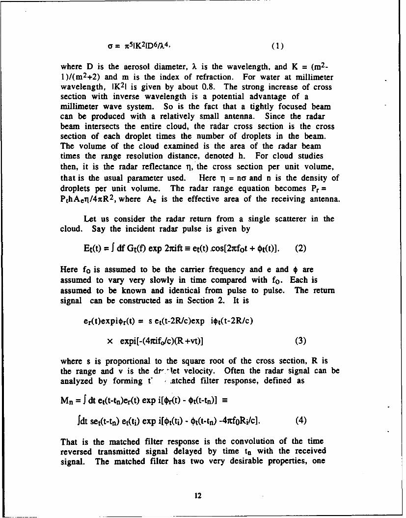
C = X5IK21D6/X4, (1)

where D is the aerosol diameter, ). is the wavelength, and K = (m2-1)/(m 2+2) and m is the index of refraction. For water at millimeterwavelength, IK2 1 is given by about 0.8. The strong increase of crosssection with inverse wavelength is a potential advantage of amillimeter wave system. So is the fact that a tightly focused beamcan be produced with a relatively small antenna. Since the radarbeam intersects the entire cloud, the radar cross section is the crosssection of each droplet times the number of droplets in the beam.The volume of the cloud examined is the area of the radar beamtimes the range resolution distance, denoted h. For cloud studiesthen, it is the radar reflectance il, the cross section per unit volume,that is the usual parameter used. Here Ti = na and n is the density ofdroplets per unit volume. The radar range equation becomes Pr =PthAeti/4xR 2 , where Ae is the effective area of the receiving antenna.

Let us consider the radar return from a single scatterer in thecloud. Say the incident radar pulse is given by

Et(t) = j df Gt(f) exp 2nift M et(t) .cos[2xrfot + ýt(t)]. (2)

Here fo is assumed to be the carrier frequency and e and 0 areassumed to vary very slowly in time compared with fo. Each isassumed to be known and identical from pulse to pulse. The returnsignal can be constructed as in Section 2. It is

er(t)eXPibr(t) = s et(t-2R/c)exp i&t(t-2R/c)

x expi[-(4nif0/c)(R +vt)] (3)

where s is proportional to the square root of the cross section, R isthe range and v is the dr', let velocity. Often the radar signal can beanalyzed by forming t' Latched filter response, defined as

Mn = I dt et(t-tn)er(t) exp i[4r(t) - Ot(t-tn)] -

Idt set(t-tn) et(ti) exp i[qt(ti) - ot(t-tn) -4nrfoRi/c]. (4)

That is the matched filter response is the convolution of the timereversed transmitted signal delayed by time tn with the receivedsignal. The matched filter has two very desirable properties, one

12

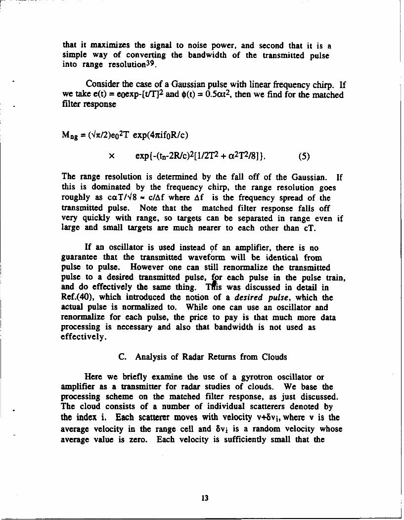
that it maximizes the signal to noise power, and second that it is asimple way of converting the bandwidth of the transmitted pulseinto range resolution 39 .

Consider the case of a Gaussian pulse with linear frequency chirp. Ifwe take e(t) = eoexp-[tfT]2 and o(t) = 0.5wt2 , then we find for the matchedfilter response

Mng = (4hx/2)eo 2T exp(4nifoR/c)

X exp{-(tn-2R/c) 2 [1/2T2 + a 2T2/8]}. (5)

The range resolution is determined by the fall off of the Gaussian. Ifthis is dominated by the frequency chirp, the range resolution goesroughly as caT/48 - c/Af where Af is the frequency spread of thetransmitted pulse. Note that the matched filter response falls offvery quickly with range, so targets can be separated in range even iflarge and small targets are much nearer to each other than cT.

If an oscillator is used instead of an amplifier, there is noguarantee that the transmitted waveform will be identical frompulse to pulse. However one can still renormalize the transmittedpulse to a desired transmitted pulse, for each pulse in the pulse train,and do effectively the same thing. TAis was discussed in detail inRef.(40), which introduced the notion of a desired pulse, which theactual pulse is normalized to. While one can use an oscillator andrenormalize for each pulse, the price to pay is that much more dataprocessing is necessary and also that bandwidth is not used aseffectively.

C. Analysis of Radar Returns from Clouds

Here we briefly examine the use of a gyrotron oscillator oramplifier as a transmitter for radar studies of clouds. We base theprocessing scheme on the matched filter response, as just discussed.The cloud consists of a number of individual scatterers denoted bythe index i. Each scatterer moves with velocity v+bvi, where v is theaverage velocity in the range cell and 8vi is a random velocity whoseaverage value is zero. Each velocity is sufficiently small that the

13

scatterers can be regarded as stationary duiing the individual radarpulse. However the velocities will be Doppler resolved by looKing atreflections from a long sequence of pulses. The return signal can beconstructed by summing over the returns from the individualscatterers. It is

er(t)eXPi4r(t) = li si et(t-2Ri/c)exp i&t(t-2Ri/c)

x expi[-(4xifo/c)(Ri +vt+8vit)] (6)

There is not a single transmitted pulse, but a large number ofpulses separated by interpulse time r. Let p be the index denotingpulse number and P be the total number of pulses in the pulse train.We now calculate the matched filter response for the pth pulse forthe nth range interval. Assuming that the pulse, in the case of anamplifier, or the desired pulse , in the case of an oscillator, isGaussian, the matched filter response is

Mnp = (4x/2)eo2T~isiexp-[(4iifo/c)(Ri+(v+6vi)p?)] (7)

where the index n denotes the range cell and p the pulse. Weassumed each droplet is at the center of the range cell, and thesummation is over the droplets in the range cell. Associated with theindex p is the Fourrier transform variable 2%z/P where z takes oninteger values from zero to P-1. Then one can define

Qn(z) = •pMnpexp2xipz/P (8)

To obtain the reflectance, one forms the summation lzlQn(z)12 = an.In addition to the summation over z, there are four othersummations over i and p and over the analogous variables j and q inthe complex conjugate summations. The summation over z is asimple summation of a geometric series and turns out to be equal toP if p=q and zero otherwise. We then separate the summation over iand j into a sum of two summations, one having i=j and one havingi*j. The former is a simple summation over reflectance's over theindividual droplets and has N terms in it where N is the number ofdroplets. The latter is the sum of 0.5N(N-1) terms, each one having arandom phase assuming the droplets are uncorrelated. Thus theensemble average of this summation is zero. The problem is that anysingle pulse return is not an ensemble. The rms value of asummation of N2 random phases is about N, so for each value of p,

14

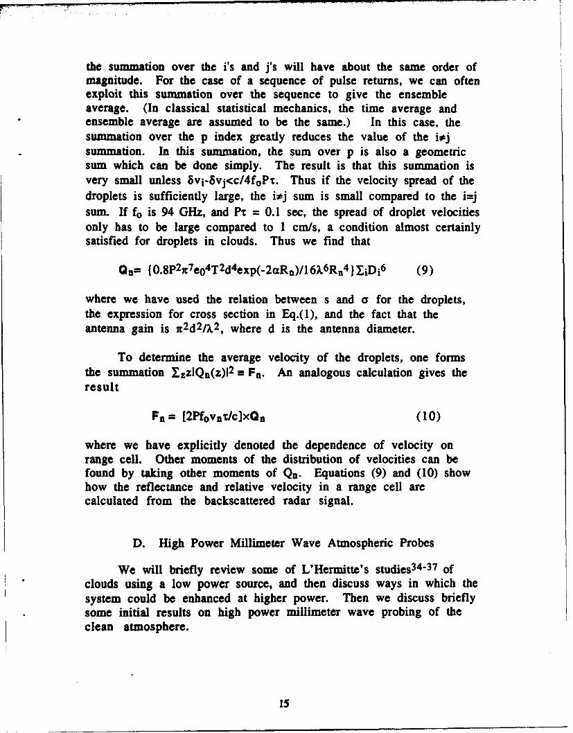
the summation over the i's and j's will have about the same order ofmagnitude. For the case of a sequence of pulse returns, we can oftenexploit this summation over the sequence to give the ensembleaverage. (In classical statistical mechanics, the time average andensemble average are assumed to be the same.) In this case, thesummation over the p index greatly reduces the value of the i*jsummation. In this summation, the sum over p is also a geometricsum which can be done simply. The result is that this summation isvery small unless 8vi-8vj<c/4f 0Pr. Thus if the velocity spread of thedroplets is sufficiently large, the i*j sum is small compared to the i=jsum. If fo is 94 GHz, and Pr = 0.1 sec, the spread of droplet velocitiesonly has to be large compared to I cm/s, a condition almost certainlysatisfied for droplets in clouds. Thus we find that

Qn= [0.8p2x 7eo4T2d4 exp(-2aRn)/16X,6Rn 4 } ]iDi6 (9)

where we have used the relation between s and a for the droplets,the expression for cross section in Eq.(1), and the fact that theantenna gain is x 2 d 2 /I. 2 , where d is the antenna diameter.

To determine the average velocity of the droplets, one formsthe summation TIzzIQn(z)12 * Fn. An analogous calculation gives theresult

Fn = [2Pfovn•'/c]xQn (10)

where we have explicitly denoted the dependence of velocity onrange cell. Other moments of the distribution of velocities can befound by taking other moments of Qn. Equations (9) and (10) showhow the reflectance and relative velocity in a range cell arecalculated from the backscattered radar signal.

D. High Power Millimeter Wave Atmospheric Probes

We will briefly review some of L'Hermitte's studies 34 -37 of

clouds using a low power source, and then discuss ways in which thesystem could be enhanced at higher power. Then we discuss brieflysome initial results on high power millimeter wave probing of theclean atmosphere.

15

L'Hermitte studied, among other things, small cumulus cloudsand intense thunderstorms, both around Miami, Florida. He does notuse an amplifier as his microwave source, but uses an oscillator. Todo the coherent signal integration and Doppler processing, he uses acoherent on receive approach and corrects the phase of the receivedsignal according to the phase of the transmitted signal4 1 . Except forthe random phase from pulse to pulse, the EIO has extremely goodsignal properties. In fact, this was the reason for Lhermitte's choiceof an EIO over a magnetron, which could operate at somewhat higheraverage power.

For a typical cumulus cloud, like those studied by L'Hermitte,the droplet diameter is about 10im and the droplet density is about100cm- 3 , so the reflectivity is about 3x10- 12 cm-1. With such smallreflectance's and low power of the transmitter, the observation of thecloud is difficult. For Lhermitte's case, with a range of 2 kin, atransmitted power of 1 kW, a range resolution distance h of 6x10 3

cm, and an effective aperture of 4x10 3 cm 2 , the received power isabout 10-13 W. The noise power of an ideal receiver at 3000K isabout 10- 14W if the bandwidth is pulse length limited to 2x10 6 s-1.However Lhermitte's receiver has an actual noise of about 5x10- 13 .His signal power is below the noise power, and he had to integratethe signal over a considerable number of pulses to get good data. Inhis case, he runs the EIO at about 10 kHz pulse repetition rate andintegrates for 3 s, or about 3x10 4 pulses. He finds that themeteorological conditions remain reasonably constant for these 3s.

One of L'Hermitte's other observations was the reflection of theradar wave from a thunderstorm in the Miami, Florida area. Therange at which he was able to operate was about 20-30 kin.However since the air at ground level was quite humid, he was onlyable to observe the tops of the clouds. For instance one of hisobservations is at an angle of 340 and a range of 20 km, so that heobserves an altitude of 11 km. He points out that at a 300 elevation,the two way absorption was 12 dB, whereas at a 70 angle, it is 50dB.

Now let us discuss the way these cloud measurements could beenhanced at higher transmitted power. For the case of thethunderstorm, the additional power could be directly used toovercome absorption in the humid air. For instance a 4 kW averagepower system would overcome an additional 30 dB of atmosphericabsorption and allow observation much lower in the thunderstorm.

16

Now consider the observation of the cumulus cloud. A smallcloud passes directly overhead at an altitude of about 1.5 kin; as itgoes by, the reflectivity and vertical velocities are measured by theradar at a series of range cells 65 m in depth. The cloud is overheadfor about 2 minutes. Since each vertical scan takes 3 s, there areabout 40 vertical scans in the cloud and about 6-8 range cells. Ahigher power transmitter could enhance these measurements in anumber of ways. First, in doing the same measurement asL'Hermitte at higher power, the radar beam could be scanned fromside to side in the cloud so that a three dimensional image of thecloud could be formed. Second, the range cell could be reduced toperhaps 10 m (a 10 MHz bandwidth) so that the cloud could beexamined vertically in much greater detail. Third, the higher powercould be used for greater range to image clouds that are not directlyoverhead. This not only gives another view of the cloud, but it alsogives another component of velocity. For clouds with a horizontalrange of perhaps 10 kln, the radar would give a Doppler velocity in adirection that is almost horizontal.

The other very important application for 94 GHz cloud radarstudies is the proposed space based radar. Here the power requiredis greater than the 4 Watt system used up to now. Finally DavidAtlas4 2 ,4 3 has recently pointed out a number of fundamental issueswith regard to cloud dynamics that can be effectively studied with94 GHz radars. Some of these issues are enumerated in Table 2.

We conclude by discussing a recent experiment on probing theclear atmosphere with a high power 84 GHz gyrotron44 . Theexperiment was cw and the transmitter had a power of 10 kW. Thereceiver had a sensitivity of 5x10 14 W, and the returned signal wasenhanced by using a 10 second integration time. The transmittedbeam was scanned in angle, and at certain angles, there were strongbackscattered signals. It is most likely that these signals are theresult of particulates, probably at the top of the atmosphericinversion layer, at 100-300 meters altitude. Clear air turbulence wasa possible scatterer, but if so, the turbulence would have had to beextremely intense to give rise to scatter at such small wavelength.Additional experiments are planned in the future to furtherinvestigate these phenomena.

17

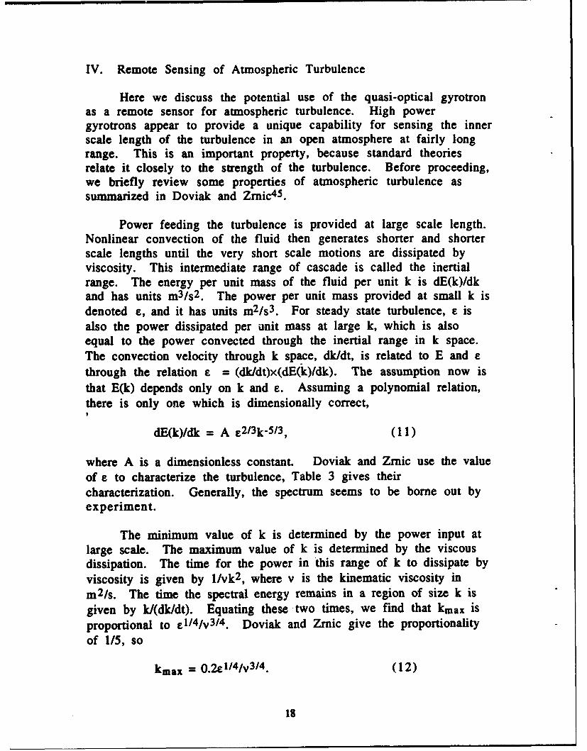
IV. Remote Sensing of Atmospheric Turbulence

Here we discuss the potential use of the quasi-optical gyrotronas a remote sensor for atmospheric turbulence. High powergyrotrons appear to provide a unique capability for sensing the innerscale length of the turbulence in an open atmosphere at fairly longrange. This is an important property, because standard theoriesrelate it closely to the strength of the turbulence. Before proceeding,we briefly review some properties of atmospheric turbulence assummarized in Doviak and Zrnic45 .

Power feeding the turbulence is provided at large scale length.Nonlinear convection of the fluid then generates shorter and shorterscale lengths until the very short scale motions are dissipated byviscosity. This intermediate range of cascade is called the inertialrange. The energy per unit mass of the fluid per unit k is dE(k)/dkand has units m3/s 2 . The power per unit mass provided at small k isdenoted e, and it has units m2 /s 3. For steady state turbulence, e isalso the power dissipated per unit mass at large k, which is alsoequal to the power convected through the inertial range in k space.The convection velocity through k space, dk/dt, is related to E and rthrough the relation e = (dk/dt)x(dE(k)Idk). The assumption now isthat E(k) depends only on k and e. Assuming a polynomial relation,there is only one which is dimensionally correct,

dE(k)/dk = A e2/3k- 5/3, (1 1)

where A is a dimensionless constant. Doviak and Zrnic use the valueof e to characterize the turbulence, Table 3 gives theircharacterization. Generally, the spectrum seems to be borne out byexperiment.

The minimum value of k is determined by the power input atlarge scale. The maximum value of k is determined by the viscousdissipation. The time for the power in this range of k to dissipate byviscosity is given by l/vk 2 , where v is the kinematic viscosity inm 2/s. The time the spectral energy remains in a region of size k isgiven by k/(dk/dt). Equating these two times, we find that kmax isproportional to 1/4/v3/ 4 . Doviak and Zrnic give the proportionality

of 1/5, so

kmax = 0.2E1/4/v 3/4 . (12)

18

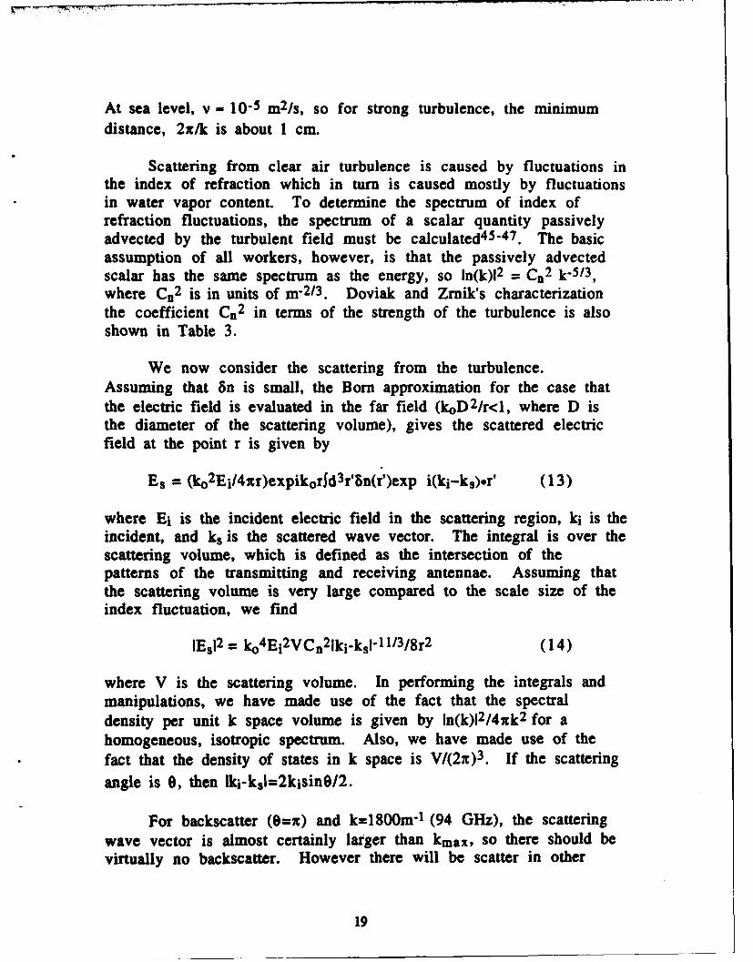
At sea level, v - I0-5 m2/s, so for strong turbulence, the minimumdistance, 2x/k is about I cm.

Scattering from clear air turbulence is caused by fluctuations inthe index of refraction which in turn is caused mostly by fluctuationsin water vapor content. To determine the spectrum of index ofrefraction fluctuations, the spectrum of a scalar quantity passivelyadvected by the turbulent field must be calculated4 5-4 7 . The basicassumption of all workers, however, is that the passively advectedscalar has the same spectrum as the energy, so In(k)12 = Cn2 k-5/ 3 ,where Cn2 is in units of m-2 /3 . Doviak and Zrnik's characterizationthe coefficient Cn2 in terms of the strength of the turbulence is alsoshown in Table 3.

We now consider the scattering from the turbulence.Assuming that 8n is small, the Born approximation for the case thatthe electric field is evaluated in the far field (koD2 /r<l, where D isthe diameter of the scattering volume), gives the scattered electricfield at the point r is given by

Es = (ko2Ei/4xr)expikorjd 3r'Sn(r')exp i(ki-ks)or' (13)

where Ei is the incident electric field in the scattering region, ki is theincident, and ks is the scattered wave vector. The integral is over thescattering volume, which is defined as the intersection of thepatterns of the transmitting and receiving antennae. Assuming thatthe scattering volume is very large compared to the scale size of theindex fluctuation, we find

1Esj 2 = k04 Ej2VCn21kj-k3 1 11/3 18r 2 (14)

where V is the scattering volume. In performing the integrals andmanipulations, we have made use of the fact that the spectraldensity per unit k space volume is given by In(k)12/4xk 2 for ahomogeneous, isotropic spectrum. Also, we have made use of thefact that the density of states in k space is V/(2x)3. If the scatteringangle is 0, then Iki-ks5 =2kisin0/2.

For backscatter (O=x) and k=l800m"1 (94 GHz), the scatteringwave vector is almost certainly larger than kmax, so there should bevirtually no backscatter. However there will be scatter in other

19

directions. The use of powerful gyrotrons at 94 GHz (and possibly at35 GHz also) opens up the possibility of examining the inner scalelength by oblique scattering measurements. The inner scale lengthcould be inferred from the angle at which the scattering disappears.

Let us consider a specific example to show how the availabilityof 94 GHz gyrotrons with over 100 kW of power can render possiblea scattering measurement of the inner scale length. The scatteringvolume is then roughly LD 2 where L is the length of the intersectionof the two antenna patterns and we have assumed the incident beamis the more tightly focused of the two. Then we relate the fieldamplitude to the power density and add to Eq.(14) additional factorsaccounting for the atmospheric attenuation. Then Eq.(14) can berewritten as

Pr = k04 AeLPtCn21kj-ks 1"11/3 exp[-a(ri+rs)]/8rs 2 (15)

where Pr(t) is the incident (reflected) power, Ae is the aperture ofthe receiving antenna, a is the atmospheric attenuation, and ri is therange from the incident antenna to the scattering region. Let uschoose a configuration in which the scattered radiation is in the farfield. Although this is not absolutely necessary, it does simplify boththe analysis and the interpretation of any data.

Take a transmitting antenna of D=3 m which can focusradiation down to a spot 2 m, 2.5 km away, and a range to thereceiver of 10 kmn. For relative humidity 50% or less, the attenuationis 10 dB or less. For 94 GHz radiation with a 3 m receiving antennaand an assumed inner scale length of 3 cm (Iki-ksI=200), we find thatPr/Pi- 2x10- 17 , assuming strong turbulence, Cn=3x10"13, and alsoL=D/sin0. If the incident power is 105 W, the received power isabout 2x10- 12 W, 4 times the noise power at 3000K. Integrationover a small number of pulses could further enhance SNR. Considerthe alternative of using an EIO having a power of 1 kW and anaverage power of 4 W. Now the signal is a factor of 25 below thenoise level, and this is for fairly strong turbulence. It is unlikely thatthe SNR could be significantly increased by integrating over a largenumber of pulses; at the shortest scale length (3 cm), the correlationtime of the turbulence is undoubtedly very short (10- 2 s at 3m/s), sothe scattered pulses would not be coherent with one another for verylong.

20

A configuration for bistatic remote sensing of clear airturbulence is shown in Fig. 17. A transmitter is on the ground adistance D from the receiver. It points upward at a shallow angle *.The receiver also focuses to a point at which it intersects thetransmitted beam at an altitude h. By varying the direction of thetransmitted beam, the angle 0 between the transmitted and receivedbeam varies, and the scattering can be determined as a function ofthis angle.

21

V. Remote Sensing of Trace Impurities in the Upper Atmosphere

We now look into whether the tunability of the quasi-opticalgyrotron can be used to detect trace elements. At sea level, thisappears to be an extremely difficult measurement due to the factthat the pressure broadening of the absorption lines is substantial(typically about 2-3 GHz), and the impurity concentration is verylow. That is the absorption rate at the line center scales as thenumber density of the impurity in question Ni divided by thecollision rate, which is in turn proportional to the ambient density Na;so that the absorption rate is proportional to Ni/Na. At sea level, Nais very large, so the absorption rate is correspondingly small.Distinguishing the impurity absorption from the water vaporabsorption, which dominates it by many orders of magnitude, doesnot appear to be a simple task. However for impurities in the upperatmosphere, the pressure broadening is much less, so Ni/Na is muchgreater. Also there is much less water vapor at high altitude tointerfere with the measurement.

The idea is then to use a high power tunable source to do anabsorption (and possibly also phase shift) measurement as a functionof frequency near the absorption line., (One might think that at highaltitude, the molecule would spontaneously re-emit before it iscollisionally de-excited. However the time for spontaneous re-emission for rotationally excited molecules varies from about 104 to109 s, so this is not the case4 8 .) Measurements like this are currentlyperformed by radiometry, either ground or space based, wherebythe thermal spectrum of the atmosphere is measured and related tothe trace elements. An alternate scheme is to use a millimeter wavesource at high power to selectively (as a function of frequency) heatthe upper for diagnostic purposes.

A. Trace Element Determination by Radiometry

In radiometry, the thermal spectrum of millimeter waveradiation is detected and related to the concentration of theelement. 4 8 These measurements can be absorption measurements,for instance measuring the absorption of sunlight at frequencies nearthe absorption line. Also the thermal emission can be studied, andthis is what we concentrate on here. For the atmosphere whichradiates as a black body (if it were optically thick) the radiationtemperature is related to the intensity of radiation by the Rayleigh-Jeans, or actually the Planck law. If the radiation is emitted from a

22

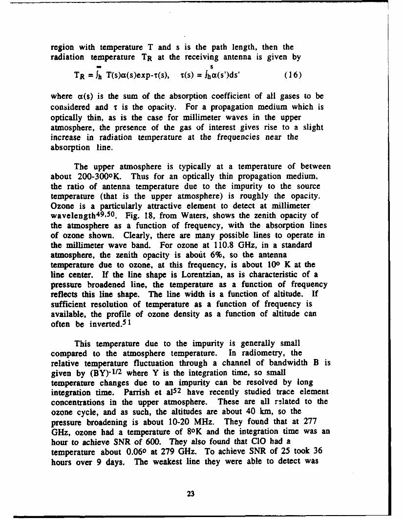
region with temperature T and s is the path length, then theradiation temperature TR at the receiving antenna is given by

- STR = Jh T(s)a(s)exp-r(s), er(s) = Jha(s')ds' (1 6)

where a(s) is the sum of the absorption coefficient of all gases to beconsidered and r is the opacity. For a propagation medium which isoptically thin, as is the case for millimeter waves in the upperatmosphere, the presence of the gas of interest gives rise to a slightincrease in radiation temperature at the frequencies near theabsorption line.

The upper atmosphere is typically at a temperature of betweenabout 200-300oK. Thus for an optically thin propagation medium,the ratio of antenna temperature due to the impurity to the sourcetemperature (that is the upper atmosphere) is roughly the opacity.Ozone is a particularly attractive element to detect at millimeterwavelength 4 9 ,5 0 . Fig. 18, from Waters, shows the zenith opacity ofthe atmosphere as a function of frequency, with the absorption linesof ozone shown. Clearly, there are many possible lines to operate inthe millimeter wave band. For ozone at 110.8 GHz, in a standardatmosphere, the zenith opacity is about 6%, so the antennatemperature due to ozone, at this frequency, is about 100 K at theline center. If the line shape is Lorentzian, as is characteristic of apressure broadened line, the temperature as a function of frequencyreflects this line shape. The line width is a function of altitude. Ifsufficient resolution of temperature as a function of frequency isavailable, the profile of ozone density as a function of altitude canoften be inverted. 5 1

This temperature due to the impurity is generally smallcompared to the atmosphere temperature. In radiometry, therelative temperature fluctuation through a channel of bandwidth B isgiven by (BY)-1/2 where Y is the integration time, so smalltemperature changes due to an impurity can be resolved by longintegration time. Parrish et a15 2 have recently studied trace elementconcentrations in the upper atmosphere. These are all r-.lated to theozone cycle, and as such, the altitudes are about 40 km, so thepressure broadening is about 10-20 MHz. They found that at 277GHz, ozone had a temperature of 80K and the integration time was anhour to achieve SNR of 600. They also found that CIO had atemperature about 0.060 at 279 GHz. To achieve SNR of 25 took 36hours over 9 days. The weakest line they were able to detect was

23

the 266 GHz line of H02. This line had a temperature of about0.0150K and took 55 hours to resolve the line. Shown in Fig 19a isthe result for ozone, and in Fig 19b is the result for CIO from Parrishet al.

Space based millimeter wave radiometry has demonstrated thecapability of measuring simultaneously the ozone and CIO profile,world wide in real time. Waters5 3 has presented beautiful images ofCIO masses moving around the world and devouring ozone. The realtime images in Ref 23 change on a time scale faster than the timerequired for Parrish's measurement. Thus space based passivemillimeter wave radiometry appears to be the only way to get thetime resolution over the time scales of interest. However thesemeasurements are themselves limited in some ways also. To get aworld wide picture of the ozone concentration requires an averageover altitude, and to get a dependence on altitude requires anaverage over a large portion of the earth's surface taken over manyorbits. Also the radiometers on the space craft are set at 4frequencies, so that the trace impurities to be studied are set at theoutset and cannot easily be varied, at least those used in Ref. (53).Shown in Fig. (20) are horizontal images of CIO taken over 9 days,taken from Waters et al. Figure 21 shows average vertical profiles ofCIO from Ref. 53, where the data is averaged over space and time.

We now discuss the potential use of a tunable quasi-opticalgyrotron to do an active measurement of upper atmosphere traceelement impurities. There appear to be two basic types ofmeasurements one can do, incoherent or coherent. In the former, thephase information is somewhere lost on the radiation path, and inthe former it is not. Finally there is the possibility of using thequasi-optical gyrotron at high average power for selective heating ofthe upper atmosphere due to power absorption on a particularmolecular rotation line.

B. Trace Element Detection by Incoherent Scatter

We now consider the use of a high power tunable source formeasurements requiring one or two way transmission and detectionof radiation at a set of frequencies near the absorption line. Themost natural two way transmission path is reflection from the moon,which is visible from any point on earth about half the time. Wespecifically envision the use of a quasi-optical gyrotron, withtunability from 80-260 GHz. The radiation will be transmitted from

24

a ground station on earth and received in a large number ofreceivers.

The moon subtends an angle of about 10-2 radians as seen fromthe earth. We would like to focus the radiation on as small aspossible a spot on the moon, so that the range variation to the target,and thereby the temporal spreading of the reflected pulse isminimized. At 150 GHz, a 2 meter dish can focus the radiation toabout 10% of the moon's diameter; a 20 meter diameter millimeterwave qualified satellite tracker can focus the radiation to about 1% ofthe moon's diameter. Let us assume that the radiation is reflecteddiffusely from the surface of the moon into a solid angle of about xradians. Take for the radiated power, 300kW and the pulse length,10 gts. Since the range is about 4x10 8 meters, the received power ina 2 meter dish is about 4x10- 13 W assuming 10 dB attenuation on thetwo way path. If the noise temperature of the receiver is about 103degrees Kelvin and its bandwidth is about 105 s-1, the signal to noiseratio on a single pulse is about 400.

Thus the signal is quite a bit above the noise. However themoon is a rough surface. That is the surface scattered radiation isdescribed by for instance Eq.(6), where the si is now a scatteringelement on the surface. The problem is that as the frequencychanges from say the center to the wings of the absorption line, thesescattering elements change phase in an essentially random mannerdue to the fact that as the frequency varies through the absorptionline (at least a few tens of MHz), the phase of the scatterers arerandomized. Thus in any two measurements, there are order unityvariations between the two received signals if the measurements areuncorrelated. The way to resolve the absorption line then is to doan ensemble of measurements. If each measurement is uncorrelatedwith every other one, the relative error for N measurements isroughly N-1/ 2 . To decorrelate the measurements, one would usedifferent reflection points on the moon. (If the measurements arepartially correlated with one another, the fall off in relative errorwith N is slower than N- 1/2 )5 4 . For uncorrelated events, thestatistical properties are basically the same as for radiometry; thisscheme might be considered radiometry at large signal strength.

Thus for the case of ozone, where the two way zenith opacity isabout 12% at 110.8 GHz, roughly l04 pulses would be required togive signal to noise ratio of 10 from the center to wing of the

25

absorption line. For a single frequency, this would take about asecond. To resolve the line into ten frequency bands would takeabout 10 seconds. For the case of CIO, the two way opacity at 278.63GHz is about 6xl0-4 , assuming an ambient temperature of 2000K. Inorder to get a signal to noise ratio of 10-4, about 108 shots areneeded. If the rep rate is 104, f = 278.63 GHz, and the parametersare otherwise as above, then about 3 hours are needed for eachfrequency on the line. The times here are roughly the same as forpassive radiometry, but a much less sensitive receiver is needed.

Now consider the receivers on the ground. To achieve worldwide coverage, there would have to be one transmitter, most likelyon a mountain top so as to reduce the water absorption of thetransmitted radiation on the way up, and a large number of receiverson the ground. Wherever possible the receivers would be placed atas high an altitude as possible, and receivers could even be air basedfor certain measurements. Since the quasi-optical gyrotron istunable from about 80-260 GHz, a large number of differentimpurities could be measured simply by tuning the source. Thus therecent availability of powerful millimeter wave sources open thepossibility of ground based, simultaneous, world wide measurementsof upper atmosphere impurities. This7 is illustrated in Fig. 22a.

C. Trace Element Detection by Coherent Absorption Measurements

We now consider coherent scattering. This can beaccomplished first by one way propagation, that is the tunablemillimeter wave source on a satellite and the receivers on theground, or vice versa. Alternatively it can be accomplished by twoway propagation. Here, millimeter waves are reflected from asatellite, and the absorption and phase shift as a function offrequency across the absorption line provides information regardingthe trace elements in question.

We now consider the use of the quasi-optical gyrotron as atunable source for active detection of ozone. We consider the 110.8GHz absorption line; a frequency at which the quasi-optical gyrotroncan easily be tuned. To provide a two way path, we exploit reflectionfrom an existing satellite. There are many satellites and pieces ofspace debris whose low earth orbits are known to high precision.As we will see however, not all are suitable as reflectors; to be aviable reflector, the size of the satellite must be quite small.

26

In active probing of the upper atmosphere, both amplitude andphase are available to analyze. Here we consider only the phase,since the analysis of the amplitude is no different in principle fromradiometry. For a Lorentzian line shape centered at cOo, the totalcomplex attenuation and phase shift, E for the two way propagationis given by

= V{ (v + i(o-€Oo))/(v2 + (Co-w0w) 2)}, (17)

where r/v is the two way opacity at the line center, and v is thepressure broadening. At the altitude in question, v/27E is about 10MHz. Thus, for ozone, whose two way zenith opacity is 12%, andwhose opacity at 450 is about 20%, the total phase shift as onecrosses the line could be as high as 10o-150. If the incident wave isat frequency fi the phase of the returned signal is given by

*ri= 2xR(2fi+8fdi)/c + ýti(t-2R/c) + A)i(fi)

+ A6i(fi+8fdi) +0 +80(fiP) (18)

For a satellite of known orbit, the Doppler shift can becalculated very accurately, and can be as high as a few MHz for 100GHz incident radiation. In Eq.(18), A~i(fi) is the ozone generatedphase shift at frequency fi on the way up, A~i(fi+Sfdi) is the ozonegenerated phase shift of the Doppler shifted wave on the way down,0 is the phase shift from all other components, determined from forinstance a standard atmosphere model and is assumed to vary onlyslightly across the absorption line, and 80(fi,p) is the phase shiftgenerated by the satellite, where p denotes pulse number. Thesatellite generated phase shift varies with frequency becausedifferent frequencies have different scattering centers; it varies withp because the satellite might change its orientation, due to rotation,during the pulse train. The difficulty is that 80(fi,p) is basicallyunknown. One can only perform the measurement if 86(fi,p) isindependent of both fi and p.

The satellite will be considered to be a set of discretescatterers, with index m, centered at R and having position 8Rm fromthe center. It is the 8Rm's which contribute the essentially randomnature of the phase. If the frequency difference between the waves

27

in the spectrum is denoted 6f, then the contribution to the phase shiftis 4xSRUf/c, where for convenience, we have deleted subscripts. Aslong as this is small compared to the phase shift we are attempting tomeasure, it can be neglected. This then puts a limit on both the sizeof the satellite and also on the frequency spread. For ozone at 40 kmaltitude, assume a width of 20 MHz. At a 450 inclination angle, thephase shift we are measuring is about 0.2 radians. This means thatthe satellite or debris radius must be small compared to about 30 cm.Also, the phase might change pulse to pulse because of the rotationof the satellite, so the total measurement time must be smallcompared to a rotation period of the satellite, typically tens ofseconds. Thus, a small existing satellite or piece of space debris,which is not rotating violently, could serve as a reflector for rapid,ground based ozone measurement.

We now consider what it would take to do an ozonemeasurement at a satellite tracker. If we consider the antenna to be20 m (a gain of 87 dB), a bandwidth which is pulse time limited (105s-1), a transmitted power of 1 MW, a range of 300 km, a 5 cm radiusspherical scatterer, and a receiver temperature of 10000K, we findthat SNR is in excess of 106. This corresponds to a phase resolutionin a single pulse of about (SNR)-1/2 . "If 20 pulses within a time of atenth of a second to a second are transmitted within the 20 MHzinterrogation bandwidth, the phase shift within the absorption linecan be resolved and the ozone density can be inferred.

We now consider a method of making the measurement muchmore accurate. The satellite generated phase shift can be greatlyreduced or eliminated by the use of a specially designed satellite.Specifically, we consider the use of a spherical satellite, whose crosssection is independent of orientation, and whose cross section as afunction of frequency can be accurately calculated and measured.For trace elements such as CIO or H02, discussed in Ref. 52, the totalphase shift across the absorption line is 10-3-10-4 radians. Thus thesatellite must be smooth to about this fraction of a wavelength.However since we are considcrirf; millimeter waves, this fraction of awavelength means an optical q-,ality reflector, a standard capability.We consider specifically a 20 cm radius spherical reflector. In onerocket launch, a number of these, perhaps ten or so, could be placedinto orbit to provide nearly continual, permanent coverage. Anetwork of satellite trackers around the earth would then be able to

28

provide nearly continuous, world wide coverage of any element withan absorption line in the millimeter wave band.

It is interesting to note that the manufacture of metal sphereswith this accuracy and launching them into orbit is an establishedtechnique. Such metal spheres are made by for instance the SalemSpecialty Ball Corporation in West Simsbury, Connecticut 5 5 . Theyhave been launched into low earth orbit as calibration targets formeasuring radar cross section of space debris in the Orbit DebrisRadar Calibrated Sphere project 5 6 in 1992 and 1993. (The microntolerances in radius are required so that they can be shot into spacefrom a shuttle based explosive launcher.) The cost of launching theseballs into a sufficiently high earth orbit is not that great, as costs ofspace flights go. Launching them would cost in the neighborhood ofone million dollars.

We now consider reflection from one of these speciallydesigned satellites to measure trace impurity density. For instancethe 242 GHz CIO absorption5 2 line would be observable with thequasi-optical gyrotron at the second harmonic. It has a limbtemperature of few degrees Kelvin, and a ground temperature ofabout 0.050K looking near the horizontal. Since an activemeasurement has double the path length, we assume that at an angleof 450 to the zenith, a value of about 0.030K, or a phase shift of about3x10-4 radians. The total two way absorption, from sea level, at 240GHz, at an inclination of 450 to the zenith is less than 10 dB forrelative humidity less than 50%. If a high altitude is chosen for themeasurement, the absorption is less still. We consider first the use ofa satellite tracking station, with an antenna diameter of 20 m.Consider a receiver temperature now of 1000K, a total atmosphericattenuation of 10 dB, and a radiated power, assumed to be 300 kW atthe second harmonic. Then for a 10 gs pulse, SNR is about 6x107 .Ten pulses will then give sufficient SNR to accurately measure aphase shift l0-4 radians. To conclude, the tunability of the quasi-optical gyrotron gives a capability to rapidly measure upperatmosphere ozone concentrations with existing equipment. Withspecially designed satellites and accurate satellite tracking, it couldgive rapid measurement of trace impurities at much lowerconcentration. A schematic of the measurement technique is shownin Fig.(22b).

For what might be considered the ultimate of such a system,one could place the quasi-optical gyrotron in a high earth orbit

29

satellite, so that the radiation is focused on the entire visiblehemisphere. This would enormously increase the signal to noiseratio since now there is a one way path. The frequency could betuned to that of the absorber of interest and the signal could bereceived at a network of ground receiver stations. For instance if theinstantaneous radiated power is 100 kW, the received power througha 2 meter dish is about 10-8W, at least 6 orders of magnitude abovethe noise level for a 3000K receiver with megahertz bandwidth. Ifthe duty cycle of the source is l0-3, and the efficiency is 30%, as hasalready been demonstrated, the prime power needed for thisfunction on the satellite is only 300 W, assuming that it is radiatingall the time. While the cost of launching a high power millimeterwave source into geosynchronous, or other high earth orbit is great,it would provide a tremendous capability for rapid, altitude resolved(by the absorption line profile), worldwide monitoring virtually anyupper atmospheric impurity of interest. A schematic of this schemeis shown in Fig.(22c).

Atmospheric Modification With High Power Millimeter Waves

We now consider millimeter wave sources at the very highestachievable average power, the several hundred kilowatt to megawattlevel, and examine the possibility of atmospheric modification. Weconsider here the heating of the atmosphere by the absorption(actually the differential absorption) of this radiated power by theabsorption line of interest. Let us consider for instance the 278 GHzline of CIO, for which the opacity as measured by Parrish was about3x10"4. Let us imagine an average radiated power of 300 kW, sothat the absorbed power by the CIO would be about 100 Watts. Ifthis is radiated by a 20 meter, millimeter wave qualified dish, andthe CIO which does the absorption is spread out between about 30and 40 kin, this then gives an additional heating rate in the radiationbeam of about 10-5 degrees Kelvin per second. If the loss is due tothermal conduction to the cooler gas outside of the beam, thetemperature rise of the gas in the beam would be limited to about20K. As we have seen, this temperature raise can be measured byconventional radiometry along the boresight. For ozone, a 110.8GHz, the power required to measurably heat the atmosphere arevery much less. Thus by using the tunable millimeter wave source,at its highest average power to heat the atmosphere, one can detectelements with as low a density as that of CIO.

30

VI. Atmospheric Sensing With Free Electron Lasers

The field of remote sensing of the atmosphere with lasers is anenormous 2 ,57 one and we will only give a very brief discussion here.As is apparent in Fig. (2), FEL's, if they could be portable and fielded,could give a breakthrough capability in the infrared for the case thattunability is required. Tunability is required mostly for differentialabsorption lidar (DIAL). Here the absorption of laser light iscompared at the center and far from the absorption line of animpurity in question. A measurement of differential absorption thenallows one to infer the concentration of the impurity. There aremany possible configurations. First there can be a two point pathmeasurement or a measurement at a single point where a remotereflector has been placed. For either of these, there has to be acooperative position remote from the laser. Secondly, the reflectioncan be from some typographical object, a building, tree or hillside.Since the reflection is diffuse, this second approach generallyrequires more transmitted power. In either case, what one ends upwith is path integrated concentration of the impurity. A thirdapproach is to use the existing atmospheric aerosols as the scatteringmechanism. Here the impurity concentration can be range resolved,but the transmitted power requirement is larger still. Furthermore,since the reflector is rough and the propagation is affected byatmospheric turbulence, the measurement is only meaningful whenaveraged over a large number of laser pulses.

There are many possible impurities which could be detectedwith IR DIAL, but the field is hampered by a lack of tunable,powerful lasers. To quote Fredriksson 5 8"DIAL applications in themid-IR region in general, suffer from lack of tunable, high energylaser sources, and detection techniques is so far not as highlydedicated as in the UV and visible DIAL technique ........ A great dealof effort has been put into IR DIAL techniques by many researchgroups, but it is somewhat discouraging that so few fieldmeasurements have been made. However everything points to abreakthrough when well suited lasers an dedicated detectiontechniques become available."

In the infrared, the available sources are basically line tunablesources. Thus DIAL measurements have to be the result of acoincidence between one of the available laser lines and theabsorption line of the impurity in question. For a C02 laser, the linesare separated by about 50 GHz, while the atmospheric line widths

31

are typically 2-3 GHz. Thus, most of the spectral region between 9and I1 •Im is uncovered. For the case where there is a coincidence oflines, one can do DIAL measurements. For instance Killinger anMenyuk 59 used a CO 2 laser DIAL system, where the reflected beamwas from a typographic object, to detect CH4 . Shown in Fig. (23),taken from Ref.(59) are the absorption as a function of inverse wavelength for air with and without 40 ppb of CI4. Note the coincidenceof the absorption peak of CH4 with the P(14) line of the C02 laser.With their DIAL setup and reflections from a typographic object,concentrations as low as 10 parts per billion were detected over bothroads and airplane runways. Their maximum range was about 2.7km. The use of a fielded infrared FEL would open the capability ofIR DIAL, but without relying on coincidences between the particularlaser and the absorption line of the impurity in question. In additionits continuous tunability would allow not only for measurements attwo wavelengths, on and off the absorption line; but would also allowfor full resolution of the spectral line shape.

In addition to its tunability, the FEL also brings an increase inradiated power by many orders of magnitude, as is apparent fromFig.(2). This is especially true between about 3 and 9 gmwavelength, and over a larger range still if one considerscontinuously tunable power. In DIAL, the maximum range scales asthe transmitted power squared, since all of the radiated beamintersects the target. Thus FEL's have the capability of greatlyincreasing the range of DIAL systems. These ranges are currentlyrather short, hundreds of meters to a few kilometers, and integrationtimes are correspondingly long. For instance Weitkamp 60 et almeasured HCI concentration as a function of distance from anincineration ship by using a low power DF DIAL laser system. Hisresults, taken from Ref.(60) are shown in Fig. (24). The integrationtime for each plot was about an hour, and the maximum range forthe system was about 2 km. Thus if FEL's with average power oforder 100 Watts could be fielded, the entire area of IR DIAL could beripe for a breakthrough.

32

VH. Conclusion

Gyrotrons and FEL's have potential for greatly increasing thecapability of atmospheric sensors. They could extend weather radarsand lidars to new regimes of power, wavelength and tunability.Gyrotron oscillators at 94 GHz, and quasi-optical gyrotron oscillatorsor amplifiers could be fielded today. It is possible that moreconventional gyrotron amplifiers at this frequency will soon beavailable also. The development of FEL's has not yet matured to thepoint where they could be fielded, however there are severaldevelopment strategies that could lead in this direction.

33

Acknowledgement

The author would like to thank R. Lhermitte, D. Atlas, M. Sundquist,T. Ackerman, R. Presutti, J Stanley, N. Menyuk, and A. Fliflet for anumber of very useful discussions. The calculation in Fig 6 was doneby A. Fliflet. This work was supported by ONR.

34

References:

I. H. Liebe, Int. J. IR and Millimeter Waves, 10, 631, (1989)

2. D. Killinger and N. Menyuk, Science, 325, 37, (1987)

3. K. Kresicher and R. Temkin, Phys. Rev. Let,. 59. 547, 1987

4. K. Kreischer et al, Phys Fluids B2, 640, 1990

5. A. Gaponov et al, Int. J. Electronics, 51, 277, 1981

6. A. Fix et al, Int. J. Electronics, 57, 821, 1984

7. A. Bensimhon, G. Faillon, G. Garin, and G. Mourrier, Int. J.Electronics, 57, 805, 1984

8. E. Borie et al, 15th IR and Millimeter Waves Conference, Temkined, SPIE Vol 1514, p493, 1990

9. Y. Mitsunaka et al, 15th IR and Millimeter Waves Conference,Temkin, ed, SPIE Vol 1514, p318, 1990

10. H. Guo et al, IEEE Trans. Plasma Sci., 18, 326, 1990

11. A. Fliflet et al, J. Fusion Energy, 9, 31, 1990

12. K. Felch et al, Int. J. Electronics, 57, 815, 1984

13. K. Felch et al, Int. J. Electronics, 61, 701, 1986

14. V. Flyagin, A. Goldenberg, and V. Zapevalov, 18th InternationalConference on IR and MM Waves, Colchester, England, September,1993, SPIE Vol 2104, p 581

15. G. Bergeron, M. Czarnaski, and M. Rhinewine, Int. J. Electronics,69, 281, 1990

16. M Rhinewine et al, 15th IR and Millimeter Waves Conference,Temkin ed, SPIE Vol 1514, pp 578, 1990

35

17. 1.1. Antakov, E.V. Zasypkin, and E. Sokolov, 18th InternationalConference on IR and MM Waves, Colchester, England, September,1993, SPIE Vol 2104, p 466

18. A. Fliflet, R. Fischer, and W. Manheimer, Phys. Fluids B, 5, 2682,(1993)

19. R. Fischer et al, Phys. Rev. Let. to be published, 1994

20. G. Scheitrum, T. Bemis, T. Hargreaves, and L. Higgens, 18thInternational Conference on IR and MM Waves, Colchester, England,September, 1993, SPIE Vol 2104, p 523

21. T. Hargreaves, K. Kim, J. McAdoo, S. Park, R. Seeley, and M. Read,Int. J. Electronics, 57, 977, 1984

22. A. W. Fliflet, T. Hargreaves, W. Manheimer, R. Fisher, M. Barsanti,B. Levush, and T. Antonsen, Phys Fluids, B2, 1046, 1990

23. A. Fliflet, T. Hargreaves, W. Manheimer, R. Fisher, and M.Barsanti, IEEE Trans Plasma Sci, 18, 306, 1990

24. T. Hargreaves, A. Fliflet, R. Fisher, M. Barsanti, W. Manheimer, B.Levush, and T. Antonsen, Int. J. Electronics, 72, 807, 1992

25.. S. Alberti, M. Podrozzi, M. Tran, J. Hogge, T. Tran, P. Muggli, H.

Jodicke, and H. Mathews, Phy. Fluids B, 2, 2544, (1990)

26. R. Adler, Proc. IRE, 34, 351, (1946)

27. G. Ramian, in Short Wavelength Radiation Sources, P. Sprangleed, Proc. SPIE 1552, 57, (1991)

28. M. Sundquist, private communication, July, 1992

29. W. Manheimer and A. Fliflet, IEEE J. Quantum Electronics, to bepublished, 1994

30. K.D. Chan, K. Meier, D. Nguyen, R. Sheffield, T. Wang, R. Warren,W. Wilson, and L. Young, in Short Wavelength Radiation Sources, P.Sprangle ed, Proc. SPIE 1552, 69, (1991)

36

31. D. Feldman, R. Warren, W. Stein, J Fraser, G. Spalek, A. Lumkin, J.Watson, B. Carlsten, H. Takeda, and T. Wang, Nucl. Instr. Meth. Phys.Res. A259, 26, (1987)

32. T. Smitth,H. Schwettman, R. Rohatgi, Y. Lapierre, and J. Edighoffer,Nucl. Instr. Meth. Phys. Res. A259, 1, (1987)

33. G. Zorpette, EEE Spectrum, 30, 21, July, 1993

34. R. Lhermitte, J. Atmospheric aad Oceanic Tech. 4, 36, 1987

35. R. Lhermitte, IEEE Trans. Gooscience and Remote Sensing, 26,207, 1988

36. R. Lhermitte, Geophysical Res. Lett., 14, 707, 1987

37 R. Lhermitte, Geophysical Res. Lett., 15, 1125, 1988

38. T. Ackerman, private communication, September, 1993

39. M. Skolnik, Introduction to Radar Systems, McGraw Hill, 1980, p369

40. W. Manheimer, Int. J. Electronics, 72, 1165, (1992)

41. Ref 39, 106

42. D. Atlas, private communication, September, 1993

43. D. Atlas, GEWEX Workshop on Cloud Radar, June 1993, JPL,Pasadena, CA

44. Yu. Bekov, Yu. Dryagin, L. Kukin, and M. Tokmar, Radio Physics

and Quant. Electronics, to be published, 1994

45. Doviak and Zrnic, Chapters 10 and 11

46. R. J. Hill J. Fluid Mechanics, 88, 541, 1978

47. V.I. Tatarskii, Effects of the TurbulenceAtmosphere on WavePropagation, Available from US Dept Commerce, UDC 551.510, ISBN,07065 0680 4 Natl. Tech. Inf. Service, Springfield, VA

37

48. R.M. Price, Radiometer Fundamentals, in Methods ofExperimental Physics 12B, M. Meeks, ed, p 201, Academic Press,1976

49. J. Waters, Absorption and Emission by Atmospheric Gases, inMethods of Experimental Physics 12B, M. Meeks ed, p 142, AcademicPress, 1976

50. J. Waters, Proc, IEEE, 80, 1679. (1992)

51. A. Randegger, Pure and Applied Geophys. 118, 1052, 1980

52. A. Parrish, R. deZafra, P. Soloman, and J. Barrett, Radio Science,23, 106, 1988

53. J. Waters, L. Froidevaux, W. Read, G. Manney, L. Elson, D. Flower,R. Jarnot, and R. Harwood, Nature, 362, 597, (1993)

54. N. Menyuk, D. Killinger, and C. Menyuk, Applied Optics, 21,3377, (1982)

55. R. Presutti, Private communication, October, 1992

56. J. Stanley, Private communication, October, 1992

57. R. Measures ed, Laser Remote Chemical Analysis, J. Wiley, (1988)

58. K. Fredriksson, Chapter 4, Ref 57

59. D. Killinger and N. Menyuk, IEEE J. Quantum Electronics, QE17,1917, (1981)

60. C. Weitkamp, in Wastes in the Ocean, Vol 3, Wiley, New York,1981

38

Table i - Capabilities of recent Russian gyrotrons at about 94 GHz.

RUSSIAN GYROTRONS AT ABOUT 94 GHZWITH GAUSSIAN MODE OUTPUT

STRUCTURE

Frequency Power (MW) Pulse EfficiencyGHz Duration (s) %

83 0.5 1.5 37

110 0.5 1.5 35

140 0.9 0.3 36

167 0.5 0.7 30

39

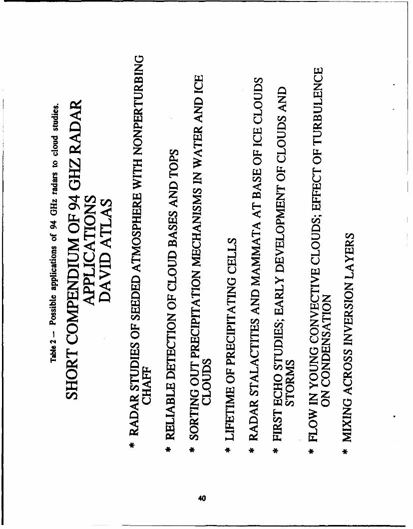
0Qzz

z

0~0

0 P"

040

zz

0 ow 0<&. U

C4 Z

0 w

40

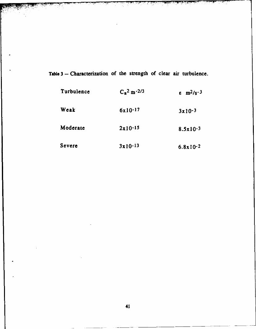
Table 3- Characterization of the strength of clear air turbulence.

Turbulence Cn2 m-2/ 3 e m2/s-3

Weak 6x10-17 3x10- 3

Moderate 2x 10- 15 8.5x10- 3

Severe 3x10- 13 6.8x10- 2

41

(a) 100h =0 km W4

E P-101.3 kPo. T-25*C

i 10

001

30

(b) E v(1OOXRH)-23.0 /lm3. 25 Curve ID fRH,% 8ops/km

0. 1 088020 2 1 885 8

3 3 8944 10 925

bJ15 5 25 991

6 so 1102 7n7 75 1212

IJ 10 8 100 1323

U)IX 55

tn 0 120 so g

- - - - - - - - - - - --5. . . . .0 50 10O0 150 200 250 300 350

FREQUENCY. GHz

Fil. 1- Millimeter wave atmospheric attenuation and phase shift as afunction of a), frequency and b), humidity, from Ref. I

42

2.D 4. .

COD

c >,I-

CV)- .-4

0) S0COC

22

00

0!!LU 0

co ~LL LI oZ40~ 0. b>.

N #4r-a

toc

I c0 0 ='

0 o

043

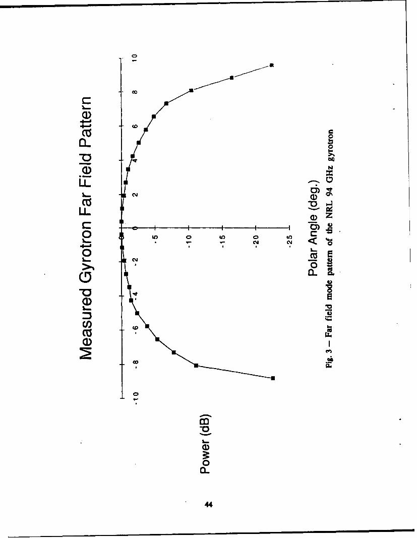
Co

czU

0 cu

-~ 0 0

LLl

0 '4-

0 L0c~Q-

(44

7-P70:

I-L

0w

o z/ 0

0 00< ~ 04.

o c

Cl) cc0

z C00 z

< -a0 0> 0

R~ Z< V)

ol0

45 z

, .144,

14

441L 1ý

40o.;,

lop

% Ar

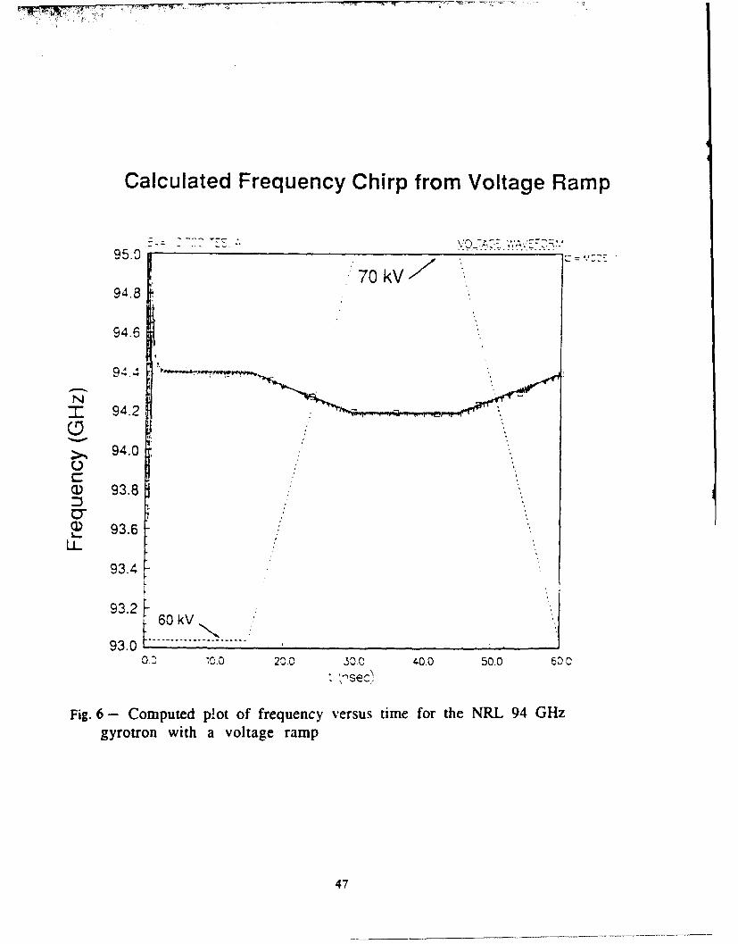
,• 2 ..•, ,• -• i .• • , •-,• ,• - • - . . . .. . ::.-. -.... ..,....

Calculated Frequency Chirp from Voltage Ramp

9 5 .0 .... .. .... ..-

•70 kVW94.8

94.6

9A.4

- 94.2

0>., 94.0

a 93.8 .

Q) 93.6

LL

93.4

60 kV

9 3 .0 -----------------------. . . '.0 10.0 20.0 .50.0 4.0.0 50.0 50 C

Fig. 6 - Computed p!ot of frequency versus time for the NRL 94 GHzgyrotron with a voltage ramp

47

woo' a

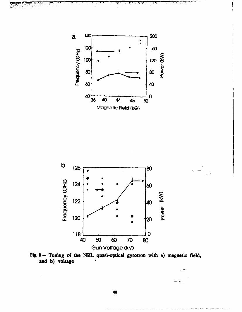
a 140 200

120 160

10oo * 120

180 80~aU 60 40

40' 036 40 44 4852

Magnetic Field (kG)

b 126 * 80

~124* 60

c 122 40

S120 6 5 2020

118 1.,_ , 0

40 50 60 70 80

Gun Voltage (kV)Fig. S - Tuning of the NRL quasi-optical gyrotron with a) magnetic field,

and b) voltage

49

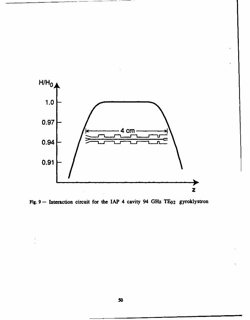
H/H0 •

1.0

0.97• ~4 cm •

0.94

0.91 •

)II

zFig. 9- Interaction circuit for the lAP 4 cavity 94 GHz TE02 gyroklystron

5o

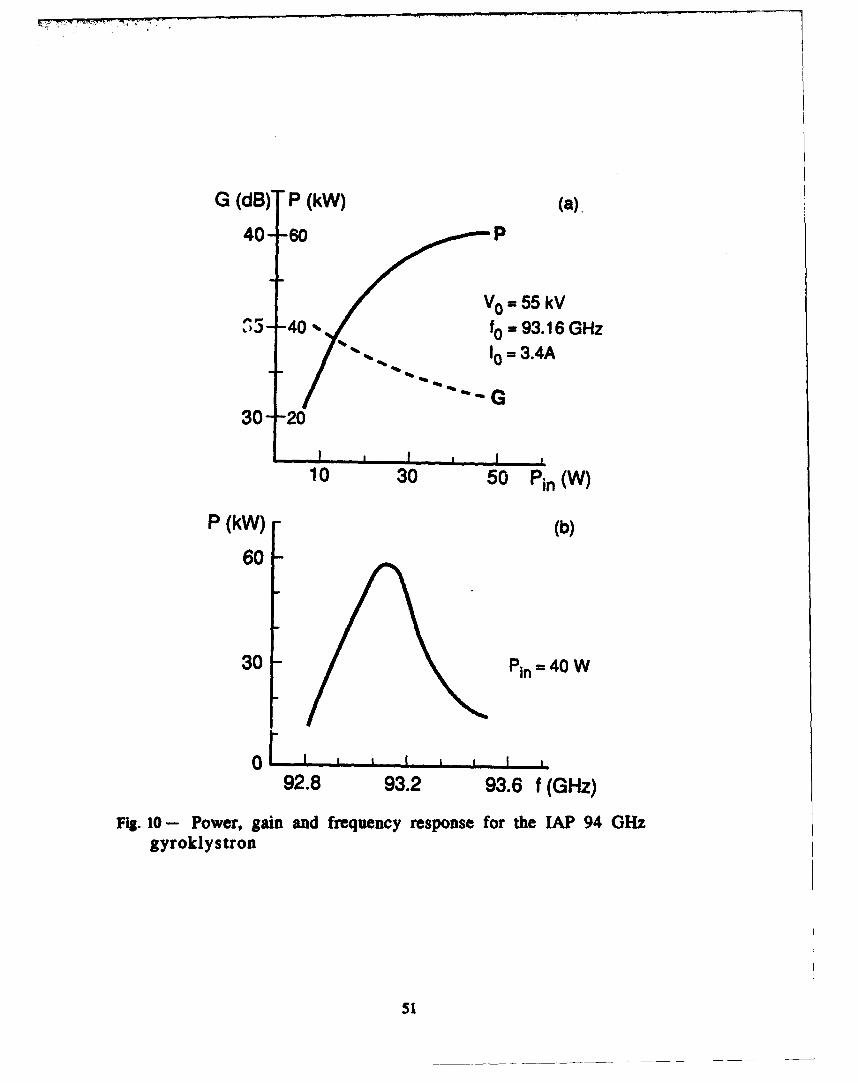
G (dB)" P (kW) (a).

40-60 P

vo = 55 WV035. -40 ,,f0 = 93.16 GHz

"-WON 10 - 3.4A

='G30-"20

I I I

10 30 50 Pin(W)

P (kW) (b)

60

30 Pin - 40 W

0 , A I I I -I L

92.8 93.2 93.6 f (GHz)

Fig. 10- Power, gain and frequency response for the UAP 94 GHzgyroklystron

51

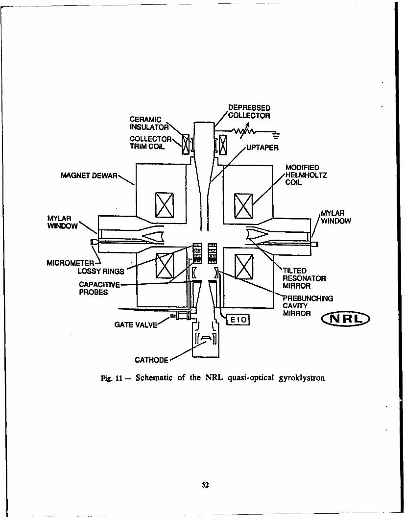
DEPRESSEDCERAMICCOLTRINSULATORCOLLECTOR

MAGNET DEWAR~N,, EMOT

MYLAR zMYLAR

MICROMETER\

RESONATORCAPACITIVE-MRO

REBUNCHING

CATHODE

Fig. 11 - Schematic of the NRL quasi-optical gyroklystron

52

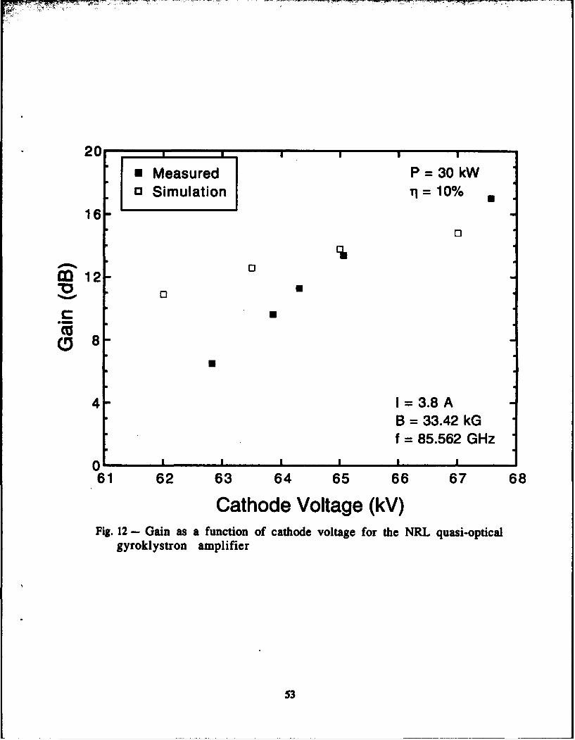
20 n n ,

* Measured P= 30 kWo Simulation ri=10%

160

IM 12"0 U

C U

S8

4 1=3.8AB = 33.42 kGf = 85.562 GHz

o I I I

61 62 63 64 65 66 67 68

Cathode Voltage (kV)Fig. 12- Gain as a function of cathode voltage for the NRL quasi-optical

gyroklystron amplifier

53

C -C

C.5"

< >

"00

Ci

0 0 0 0 d p0 d+.... I I

(8P) °l / Po

I77

oIl

o*1rII

, -•

CA,

C. . .. I'•,. - - - + i,, =

-I --,U<

56

0

!~

56

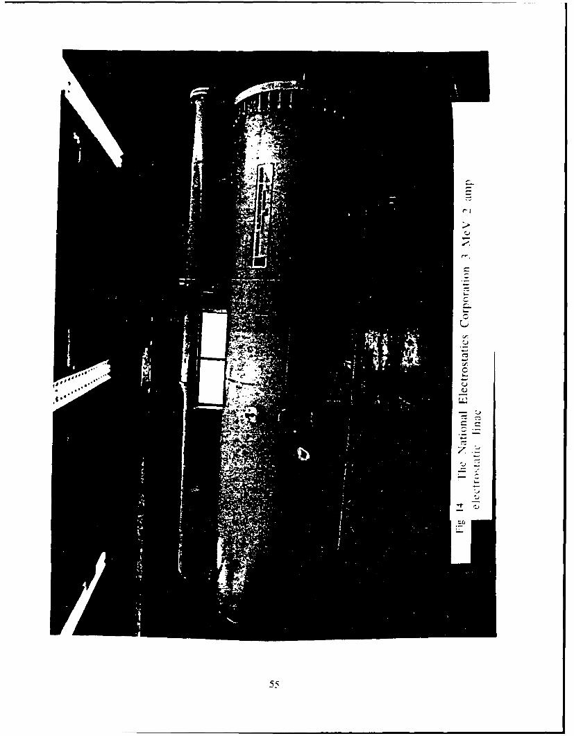
-1.

55

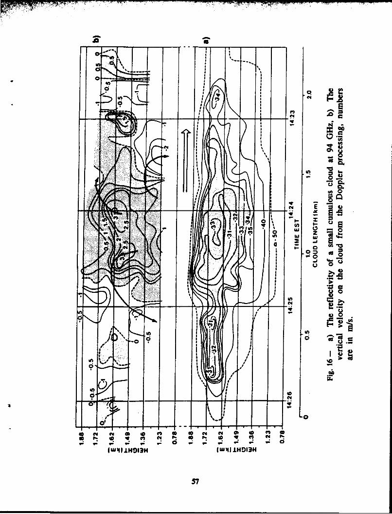
... . OldS

C4 0

d Ifl

Inq

40

ft CA V% ga CiU. r i.. . w- .; d

(wJ ill IND3H (WIIJJH913H

57

ItI-

It 2

'a:

* (dN)I AlIOVdO HIIN3Z

0 0 so '

0 V0E 0 1). C:

N 0 0

E _ _0

CP )0

01

LUJ

0 LiI e

goo

0

LL.

0 0

00

O9P) AlI3VdO N±IN3Z

5"

zU

wIL V

0=

0

N 0

4)

0 aU

0

*V

600

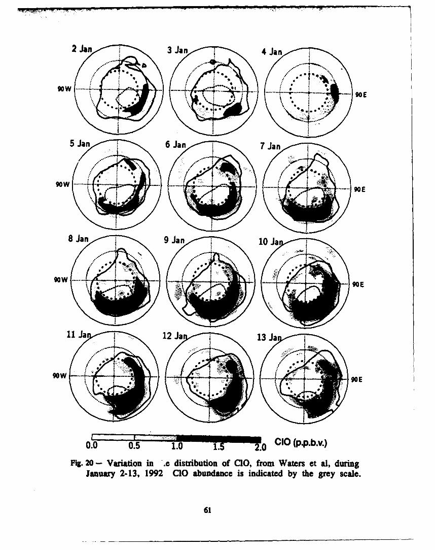
90W w~'-+0E

-% I.a6 0-4-

0.0 0. 1.0 1.5 20 CI (ab.

Fig. 20 - Variation in '.e distribution of C1O, from Waters et al, duringJanuary 2-13, 1992 CIO abundance is indicated by the grey scale.

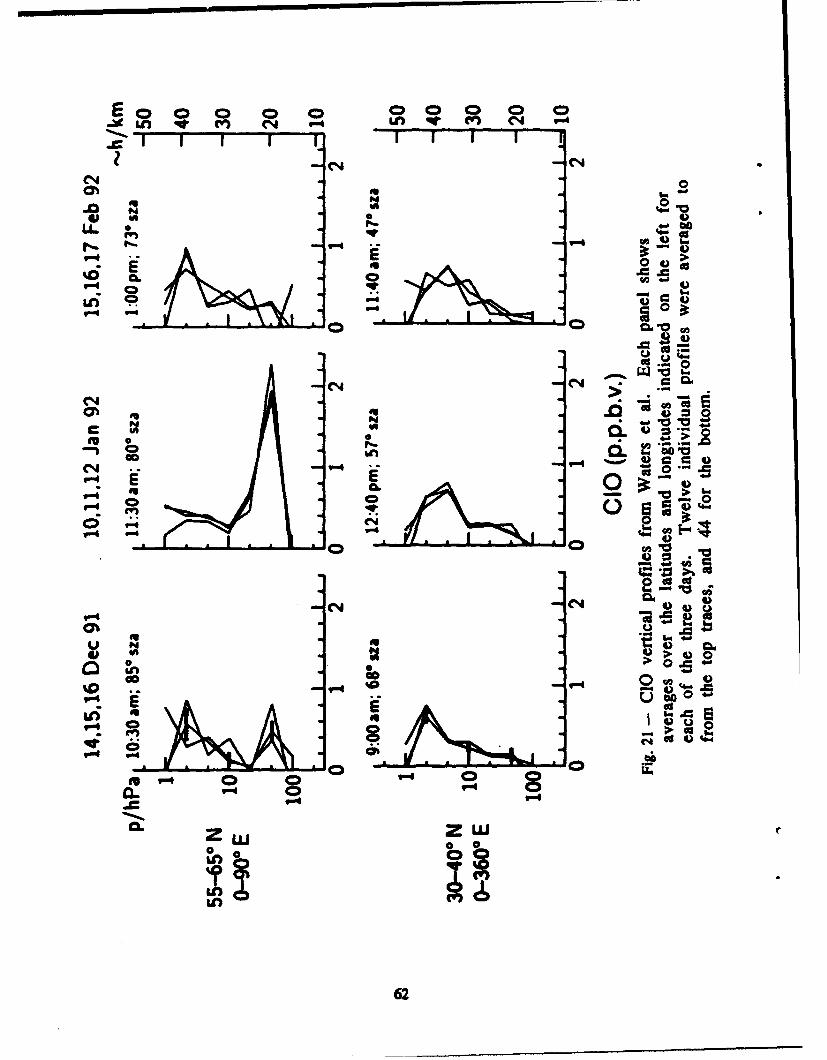
ON (

L L I' 4 .4 " 4d

0 w

0

rN CODu

"40 >

0~

~ acc4

""44

00 0

:0 ts 0

I* U *~~ I 0

62

ýT'

a

TME) OMt or &W Rsendse-

a PsWM~ lkeW NNib El E

spectrum SpICthm

b -ma ttr Space W el

detectio scheme, a)"refection rom the Roone b)reltinfo a

ax**300 km~

40 Wn

Ssruust Tracke.(mm-WOw TrMmnfttW/ReCek)

C

Fig. 22- Schematic of a variety of active upper atmosphere trace elementdetection schemes, a)'reflection from the moon, b) reflection from aspherical callibration satellite, and c) a tunable millimeter wavesource in space.

63

CO2 LASER TRANSITIONS

P(16) P(14) P(12)

1oo

CCO2 I

"" Il

Z O" 40ppb C2H40 4

LL

Z 50-4

X

T • 3-km RANGE

(n 296 K0 29-percent RELATIVE HUMIDITY

pH20

947 948 949 950 951 952

FREQUENCY (cm" I)

Fig. 23 - The coincidence of a CH4 absorption line and the line of a C02laser, taken from Ref. 26.

64

A0.

Pig.24 -Weiki0W mcS~fe~fv of 11Ci concentration as afuncion Oflf

Fi .distafl e f ro m~ an j~i fciner tio ship , take ," t 0 e . S