FAST CODES FOR MODELING THE FUSION PLASMAS RADIATIVE PROPERTIES

Gyrokinetic theory for particle transport in fusion plasmas
Matteo Valerio Falessi1,2, Fulvio Zonca3
1INFN - Sezione di Roma Tre, Via della Vasca Navale, 84 (00146) Roma (Roma), Italy
2Dipartimento di Matematica e Fisica, Roma Tre University, Via della Vasca Navale, 84 (00146) Roma (Roma), Italy
3ENEA, Fusion and Nuclear Safety Department, C. R. Frascati, Via E. Fermi, 45 (00044) Frascati (Roma), Italy
M. V. Falessi Gyrokinetic transport theory 13/06/2017 1 / 32

Introduction: purpose statement & motivations
Obtain a closed set of equations describing the dynamics of a thermonuclear plasmaon the energy confinement time of a burning plasma experiment;
By means of the equations that we are going to derive it is possible to:
study self-consistently collisional and turbulent transport;investigate structure formation on meso-scales, i.e. scale separation betweenreference state and fluctuations is not postulated;describe transport processes in realistic geometry.
M. V. Falessi Gyrokinetic transport theory 13/06/2017 2 / 32

Introduction: purpose statement & motivations
Obtain a closed set of equations describing the dynamics of a thermonuclear plasmaon the energy confinement time of a burning plasma experiment;
By means of the equations that we are going to derive it is possible to:
study self-consistently collisional and turbulent transport;
investigate structure formation on meso-scales, i.e. scale separation betweenreference state and fluctuations is not postulated;describe transport processes in realistic geometry.
M. V. Falessi Gyrokinetic transport theory 13/06/2017 2 / 32

Introduction: purpose statement & motivations
Obtain a closed set of equations describing the dynamics of a thermonuclear plasmaon the energy confinement time of a burning plasma experiment;
By means of the equations that we are going to derive it is possible to:
study self-consistently collisional and turbulent transport;investigate structure formation on meso-scales, i.e. scale separation betweenreference state and fluctuations is not postulated;
describe transport processes in realistic geometry.
M. V. Falessi Gyrokinetic transport theory 13/06/2017 2 / 32

Introduction: purpose statement & motivations
Obtain a closed set of equations describing the dynamics of a thermonuclear plasmaon the energy confinement time of a burning plasma experiment;
By means of the equations that we are going to derive it is possible to:
study self-consistently collisional and turbulent transport;investigate structure formation on meso-scales, i.e. scale separation betweenreference state and fluctuations is not postulated;describe transport processes in realistic geometry.
M. V. Falessi Gyrokinetic transport theory 13/06/2017 2 / 32

Introduction: self-consistency and spatio-temporal scales
Parameter ITERMinor radius 2.0× 10² cmIonic Larmor radius 3.2× 10⁻² cmenergy conf. time 3.5 secFluctuation frequency 2.0× 10⁴ HzCollision frequency ee 1.3× 10³ Hz
Table : Courtesy of Abel et al. 2013.
predictive simulations require collisions and fluctuations to be treated on thesame footing;on a sufficiently long time, collisions can produce a modification of the referencestate of the same order of the variation produced by fluctuations/turbulence;self-consistency is crucial also due to mutual interactions, e.g. increasedcollisional transport due to the fluctuations...
M. V. Falessi Gyrokinetic transport theory 13/06/2017 3 / 32
Introduction: what are meso-scales?
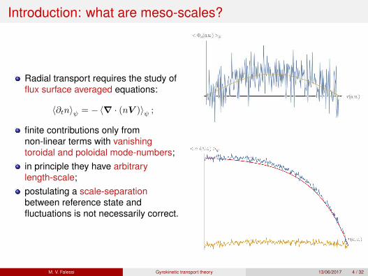
Radial transport requires the study offlux surface averaged equations:
〈∂tn〉ψ = −〈∇ · (nV )〉ψ ;
finite contributions only fromnon-linear terms with vanishingtoroidal and poloidal mode-numbers;in principle they have arbitrarylength-scale;postulating a scale-separationbetween reference state andfluctuations is not necessarily correct.
M. V. Falessi Gyrokinetic transport theory 13/06/2017 4 / 32

Introduction: outline
transport processes on the referencestate length-scale by means of themoments method;
transport processes on an arbitrarylength-scale by means of kinetictheory.
M. V. Falessi Gyrokinetic transport theory 13/06/2017 5 / 32

Introduction: outline
transport processes on the referencestate length-scale by means of themoments method;
transport processes on an arbitrarylength-scale by means of kinetictheory.
M. V. Falessi Gyrokinetic transport theory 13/06/2017 5 / 32

Gyrokinetic transport: notation
Following Hazeltine and Meiss 2003, we adopt this notation:
nV =
∫dv vf, P =
∫dv vvf, R =
∫dv
1
2mv2vvf, . . .
F =
∫dvmvC, G =
∫dv
1
2mv2vC, W =
∫dv
1
2mv2C, . . . .
Moments of the distribution function have the following evolution equations:
∂tn+ ∇ · (nV ) = 0,
∂t (nmV ) + ∇ · P − en (E + V ×B/c) = F ,
∂t
(3
2p+
m
2nV 2
)+ ∇ ·Q− enE · V = W + F · V , . . .
in principle, studying the hierarchy of moments equations is equivalent to studythe kinetic equation;long-wavelength structures are conveniently studied by means of momentsequation.
M. V. Falessi Gyrokinetic transport theory 13/06/2017 6 / 32

Gyrokinetic transport: ordering assumptions
In the core the plasma is magnetized, thus:
f = F0 + δf ρl∇ lnF0 ∼ ρl/L ∼ O(δ) 1;
perturbations have arbitrary length-scale;no scale-separation assumption between reference state and perturbations;main difference with previous works;Following Hinton and Hazeltine 1976, Frieman and Chen 1982, we describeslowly varying reference states:
ω−1 ∂
∂tln p0 = ω−1p−1
0
∂p0
∂t∼ O(δ2)
and similarly for n0, . . .
M. V. Falessi Gyrokinetic transport theory 13/06/2017 7 / 32

Gyrokinetic transport: ordering assumptions
In the core the plasma is magnetized, thus:
f = F0 + δf ρl∇ lnF0 ∼ ρl/L ∼ O(δ) 1;
perturbations have arbitrary length-scale;no scale-separation assumption between reference state and perturbations;main difference with previous works;
Following Hinton and Hazeltine 1976, Frieman and Chen 1982, we describeslowly varying reference states:
ω−1 ∂
∂tln p0 = ω−1p−1
0
∂p0
∂t∼ O(δ2)
and similarly for n0, . . .
M. V. Falessi Gyrokinetic transport theory 13/06/2017 7 / 32

Gyrokinetic transport: ordering assumptions
In the core the plasma is magnetized, thus:
f = F0 + δf ρl∇ lnF0 ∼ ρl/L ∼ O(δ) 1;
perturbations have arbitrary length-scale;no scale-separation assumption between reference state and perturbations;main difference with previous works;Following Hinton and Hazeltine 1976, Frieman and Chen 1982, we describeslowly varying reference states:
ω−1 ∂
∂tln p0 = ω−1p−1
0
∂p0
∂t∼ O(δ2)
and similarly for n0, . . .
M. V. Falessi Gyrokinetic transport theory 13/06/2017 7 / 32

Gyrokinetic transport: ordering assumptions
We introduce the following ordering for fluctuating quantities (see Frieman andChen 1982):
cE
Bvth∼ |∂/∂t||Ω|
∼∣∣∣∣δBB
∣∣∣∣ ∼ ∇‖∇⊥
∼k‖
k⊥∼ O(δ).
The ordering assumptions lead to the following relations:
f = fM +O(δ), nV ,F ,Q, [P − Ip], [R− I(5/2)p(T/m)] ∼ O(δ).
M. V. Falessi Gyrokinetic transport theory 13/06/2017 8 / 32

Gyrokinetic transport: flux coordinates
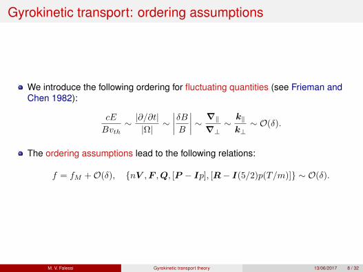
realistic geometry is crucial;flux coordinates, i.e. (ψ, θ, φ), are thenatural coordinates;
coordinate basis is (∇ψ,∇θ,∇φ);B0 = F∇φ+ ∇φ×∇ψ;equilibrium quantities do not dependon the toroidal angle φ.
Figure : Courtesy of J.Ball et al.
M. V. Falessi Gyrokinetic transport theory 13/06/2017 9 / 32
Gyrokinetic transport: flux coordinates
realistic geometry is crucial;flux coordinates, i.e. (ψ, θ, φ), are thenatural coordinates;coordinate basis is (∇ψ,∇θ,∇φ);B0 = F∇φ+ ∇φ×∇ψ;equilibrium quantities do not dependon the toroidal angle φ.
Figure : Courtesy of J.Ball et al.
M. V. Falessi Gyrokinetic transport theory 13/06/2017 9 / 32

Gyrokinetic transport: the moment approach
Taking the cross product of the force balance equation with b, see Hinton andHazeltine 1976, we obtain:
nV⊥ =1
mΩb× [∂t (nmV ) +∇ · P − enE − F ] .
Applying the ordering:
(nV⊥)1 =1
mΩb× (∇p+ en∇φ)
only information about the zeroth-order distribution function is required tocalculate the lowest order perpendicular flux;we will use this methodology to calculate second order fluxes across magneticsurfaces;distribution function must be known up to the first order to describe transportprocesses on the energy confinement time.
M. V. Falessi Gyrokinetic transport theory 13/06/2017 10 / 32

Gyrokinetic transport: density transport
In order to apply this method to descibe the transport of particles, followingHinton and Hazeltine 1976, we act with the projector R2∇φ · on the momentumequation and we take the flux surface average:⟨
R2∇φ · ∂t(nmV )⟩ψ
+⟨R2∇φ ·∇ · P
⟩ψ
=⟨R2∇φ · (enE + F )
⟩ψ
+⟨R2∇φ · (en/cV ×B)
⟩ψ.
Applying the ordering, after some calculations (see Falessi 2017), we obtain:
〈(en/c)V · ∇ψ〉ψ = −⟨(enE + F ) ·R2∇φ
⟩ψ
+
+⟨(en/c)V · (B0 −B)×R2∇φ
⟩ψ
In general the term⟨R2∇φ · ∂t(nmV )
⟩ψ
is non negligible;
only for long-wavelength structures (N.B.: different from long-wavelengthturbulence), i.e. k ∼ L−1, this term can be neglected and thus the momentmethod is convenient.
M. V. Falessi Gyrokinetic transport theory 13/06/2017 11 / 32

Gyrokinetic transport: density transport
Collisional fluxes are given by the following expressions (see Hinton andHazeltine 1976):
〈(en/c)V · ∇ψ〉ψc = −⟨F⊥ ·R2∇φ
⟩ψ
〈(en/c)V · ∇ψ〉ψNC = −⟨(enE0 + F‖) ·R2∇φ
⟩ψ.
The fluctuation induced flux is given by (see Falessi 2017):
〈(en/c)V · ∇ψ〉ψgk = −⟨(enE − enE0) ·R2∇φ
⟩ψ
+
+⟨(en/c)V · (B0 −B)×R2∇φ
⟩ψ.
These relations generalizes the derivation by Hinton and Hazeltine 1976, to anon-quiescent plasma;neoclassical transport theory is obtained as long-wavelength limit.
M. V. Falessi Gyrokinetic transport theory 13/06/2017 12 / 32

Gyrokinetic transport: density transport
〈∂tn〉ψ = − 1
V ′∂
∂ψ
[V ′ 〈nV · ∇ψ〉ψc + V ′ 〈nV · ∇ψ〉ψNC + V ′ 〈nV · ∇ψ〉ψgk
]
additive form does not imply the mutual independence of collisional and turbulentfluxes;in general fluctuations must be taken into account in the calculation of collisionalfluxes;fluctuations may enhance the deviation of system from local thermodynamicequilibrium increasing collisional transport;collisions damp fluctuation induced long lived structures which, in turn, regulateturbulent transport;at this order of the expansion, if the gyrokinetic ordering hold, it can be shown,see Sugama and Horton 1996, that the corrections to collisional fluxes arenegligible.
M. V. Falessi Gyrokinetic transport theory 13/06/2017 13 / 32

Gyrokinetic transport: density transport
〈∂tn〉ψ = − 1
V ′∂
∂ψ
[V ′ 〈nV · ∇ψ〉ψc + V ′ 〈nV · ∇ψ〉ψNC + V ′ 〈nV · ∇ψ〉ψgk
]additive form does not imply the mutual independence of collisional and turbulentfluxes;in general fluctuations must be taken into account in the calculation of collisionalfluxes;fluctuations may enhance the deviation of system from local thermodynamicequilibrium increasing collisional transport;collisions damp fluctuation induced long lived structures which, in turn, regulateturbulent transport;
at this order of the expansion, if the gyrokinetic ordering hold, it can be shown,see Sugama and Horton 1996, that the corrections to collisional fluxes arenegligible.
M. V. Falessi Gyrokinetic transport theory 13/06/2017 13 / 32

Gyrokinetic transport: density transport
〈∂tn〉ψ = − 1
V ′∂
∂ψ
[V ′ 〈nV · ∇ψ〉ψc + V ′ 〈nV · ∇ψ〉ψNC + V ′ 〈nV · ∇ψ〉ψgk
]additive form does not imply the mutual independence of collisional and turbulentfluxes;in general fluctuations must be taken into account in the calculation of collisionalfluxes;fluctuations may enhance the deviation of system from local thermodynamicequilibrium increasing collisional transport;collisions damp fluctuation induced long lived structures which, in turn, regulateturbulent transport;at this order of the expansion, if the gyrokinetic ordering hold, it can be shown,see Sugama and Horton 1996, that the corrections to collisional fluxes arenegligible.
M. V. Falessi Gyrokinetic transport theory 13/06/2017 13 / 32

Gyrokinetic transport: fluctuation induced flux
the calculation of the fluxes in termsof the distribution function requireskinetic theory;in the next slides we will calculatefluctuation-induced fluxes;in order to describe transport on theenergy confinement time we need tocalculate the distribution function upto O(δ);low frequency, i.e. ω Ω, fluctuationsare treated by means of gyrokinetics.
Figure : Courtesy of Y. Xiao et al., PoP 2015.
M. V. Falessi Gyrokinetic transport theory 13/06/2017 14 / 32

Gyrokinetic transport: pull-back
we need to express particle distribution function, i.e. f , in terms of the gyrocenterdistribution function, i.e. F ;
the gyrocenter distribution function F must satisfy F (z) = F (z) = f(z) and thefollowing relation (see Brizard and Hahm 2007, Frieman and Chen 1982):
f = e−ρ·∇F =e−ρ·∇F − e
me−ρ·∇ 〈δψgc〉
(∂F
∂E+
1
B0
∂F
∂µ
)+
+
[e
mδφ∂F
∂E
]+
[e
m
(δφ−
v‖
cδA‖
) 1
B0
∂F
∂µ+ δA⊥ ×
b
B0·∇F
]where δψgc = δφgc − v
c · δAgc = eρ·∇(δφ− v
c · δA)≡ eρ·∇δψ and 〈. . . 〉 is the
average over the gyrophase.
M. V. Falessi Gyrokinetic transport theory 13/06/2017 15 / 32

Gyrokinetic transport: pull-back
we need to express particle distribution function, i.e. f , in terms of the gyrocenterdistribution function, i.e. F ;the gyrocenter distribution function F must satisfy F (z) = F (z) = f(z) and thefollowing relation (see Brizard and Hahm 2007, Frieman and Chen 1982):
f = e−ρ·∇F =e−ρ·∇F − e
me−ρ·∇ 〈δψgc〉
(∂F
∂E+
1
B0
∂F
∂µ
)+
+
[e
mδφ∂F
∂E
]+
[e
m
(δφ−
v‖
cδA‖
) 1
B0
∂F
∂µ+ δA⊥ ×
b
B0·∇F
]where δψgc = δφgc − v
c · δAgc = eρ·∇(δφ− v
c · δA)≡ eρ·∇δψ and 〈. . . 〉 is the
average over the gyrophase.
M. V. Falessi Gyrokinetic transport theory 13/06/2017 15 / 32

Gyrokinetic transport: moments representation
The gyrophase average involves the introduction of Bessel functions as integraloperators. At the leading order:⟨
e−ρ·∇(...)⟩
= I0(...)⟨e−ρ·∇v(...)
⟩= I0v‖b(...) +
mc
eµI1b×∇(...).
where Ing(r) ≡∫dkeik·r In(λ)g(k) and In(x) ≡ (2/x)nJn(x);
using these relations we calculate the moments of the distribution functionn = 〈f〉v , nV⊥ = 〈v⊥f〉v, . . .
M. V. Falessi Gyrokinetic transport theory 13/06/2017 16 / 32

Gyrokinetic transport: moments representation
. . . obtaining the following expressions:
〈f〉v =
⟨I0
[F − e
m
(∂F
∂E+
1
B0
∂F
∂µ
)〈δψgc〉
]⟩v
+
+e
m
⟨∂F
∂E
⟩v
δφ+e
m
⟨1
B0
∂F
∂µ
(δφ−
v‖
cδA‖
)⟩v
+
+ δA⊥ ×b
B0·∇
⟨F⟩v
〈v⊥f〉v =mc
eb×
⟨µI1∇
[F − e
m
(∂F
∂E+
1
B0
∂F
∂µ
)〈δψgc〉
]⟩v
which we substitute in the fluctuation induced flux expression . . .
M. V. Falessi Gyrokinetic transport theory 13/06/2017 17 / 32

Gyrokinetic transport: fluctuation induced flux
. . . obtaining, at the leading order, the following expressions for the flux induced byelectric field fluctuations:
−⟨(enE − enE0) ·R2∇φ
⟩ψ
= e⟨R2∇φ ·∇δφ
⟨I0(λ)δG
⟩v
⟩ψ
where G = F − em∂F∂E 〈δψgc〉, and by magnetic field fluctuations:
⟨(en/c)V · (B0 −B)×R2∇φ
⟩ψ
=
e⟨R2∇φ ·
⟨∇(−v‖
cδA‖
)I0(λ)δG+ ∇
(meµδB‖
)I1(λ)δG
⟩v
⟩ψ
only symmetry breaking perturbations generate transport;these expressions can be calculated explicitly knowing the distribution functionup to the first order.
M. V. Falessi Gyrokinetic transport theory 13/06/2017 18 / 32
Gyrokinetic transport: fluctuation induced flux
. . . obtaining, at the leading order, the following expressions for the flux induced byelectric field fluctuations:
−⟨(enE − enE0) ·R2∇φ
⟩ψ
= e⟨R2∇φ ·∇δφ
⟨I0(λ)δG
⟩v
⟩ψ
where G = F − em∂F∂E 〈δψgc〉, and by magnetic field fluctuations:
⟨(en/c)V · (B0 −B)×R2∇φ
⟩ψ
=
e⟨R2∇φ ·
⟨∇(−v‖
cδA‖
)I0(λ)δG+ ∇
(meµδB‖
)I1(λ)δG
⟩v
⟩ψ
only symmetry breaking perturbations generate transport;
these expressions can be calculated explicitly knowing the distribution functionup to the first order.
M. V. Falessi Gyrokinetic transport theory 13/06/2017 18 / 32

Gyrokinetic transport: fluctuation induced flux
. . . obtaining, at the leading order, the following expressions for the flux induced byelectric field fluctuations:
−⟨(enE − enE0) ·R2∇φ
⟩ψ
= e⟨R2∇φ ·∇δφ
⟨I0(λ)δG
⟩v
⟩ψ
where G = F − em∂F∂E 〈δψgc〉, and by magnetic field fluctuations:
⟨(en/c)V · (B0 −B)×R2∇φ
⟩ψ
=
e⟨R2∇φ ·
⟨∇(−v‖
cδA‖
)I0(λ)δG+ ∇
(meµδB‖
)I1(λ)δG
⟩v
⟩ψ
only symmetry breaking perturbations generate transport;these expressions can be calculated explicitly knowing the distribution functionup to the first order.
M. V. Falessi Gyrokinetic transport theory 13/06/2017 18 / 32

Gyrokinetic transport: energy transport
Following the same methodology we obtain an equation for the energy transport:
∂t⟨p⊥ + p‖/2
⟩ψ
+1
V ′∂
∂ψ
[V ′(〈Qeff ·∇ψ〉ψ
)]= 〈W 〉ψ
where 〈W 〉ψ is a collisional heating source and:
〈Qeff ·∇ψ〉ψ ≡ 〈Q ·∇ψ〉ψ +⟨cp⊥E ·R2∇φ
⟩ψ.
The following relations hold:
〈Qeff · ∇ψ〉ψc = −(mc/e)⟨G⊥ ·R2∇φ
⟩ψ
〈Qeff · ∇ψ〉ψNC = −⟨(cE0(p⊥ + p‖/2) + (mc/e)G‖) ·R2∇φ
⟩ψ
〈Qeff · ∇ψ〉ψgk = −⟨c(E −E0)(p⊥ + p‖/2) ·R2∇φ
⟩ψ−⟨Q · (B −B0)×R2∇φ
⟩ψ
The expressions are formally the same! We can substitute the momentsrepresentation . . .The reason will be described in the next slides using a kinetic approach.
M. V. Falessi Gyrokinetic transport theory 13/06/2017 19 / 32

Gyrokinetic transport: comparison with previous works
this derivation generalize the work by Hinton and Hazeltine 1976 by includingfluctuation-induced transport;a limited amount of works have studied in a self-consistent way collisionaltransport and fluctuation induced transport. In particular Sugama et al. 1996 and,recently, Plunk 2009 and Abel et al. 2013;the derivation technique that we have used is significantly more compact andintuitive;results are consistent with previous works and they are derived in the frameworkof gyrokinetic field theory (see Sugama 2000). Therefore they can be calculateddirectly from gyrokinetic simulations;
differently from these works we did not introduce spatio-temporal averages and,consequently, scale separation assumptions;thus we have shown that postulating a separation of scales between thecharacteristic spatio-temporal scales of the reference state and of the fluctuationsis not required;in the second part of the talk we will show that this is correct only for fluctuationssuch that kL < δ−1/2 but not in the general case.
M. V. Falessi Gyrokinetic transport theory 13/06/2017 20 / 32

Gyrokinetic transport: longer time-scales
in a modern magnetic fusion device, i.e. ITER, the time scale of validity of thetransport equations that we derived is of the order of the seconds;short compared the expected duration of a pulse, i.e. > 3000s...predictive simulations require an accuracy up to O(δ3) on the fluxes and up toO(δ2) on the distribution function;it would be useful to extend this derivation up to the next order...
anyway the equations already derived could be used to build actuators based onreduced models for the real time control of plasma dynamic evolution.
M. V. Falessi Gyrokinetic transport theory 13/06/2017 21 / 32

Gyrokinetic transport: longer time-scales
Extending this derivation to longer timescales requires to modify the:
Fluctuation induced fluxesconceptually clear, see Brizard and Hahm 2007;an expression for the pull-back operator correct up to O(δ2) is required;in principle derived by means of gyrokinetic field theory (see Sugama 2000);not yet derived for electromagnetic fluctuations.
Collisional fluxesclassical and neoclassical transport theories provide a framework to derive linearrelations connecting the thermodynamic forces and the fluxes satisfying Onsagersymmetry;higher order terms, in principle, may lead to non-linear closure relations;non-linear closure relations can be studied by means of Thermodynamic FieldTheory, see Sonnino 2009.
M. V. Falessi Gyrokinetic transport theory 13/06/2017 22 / 32

Gyrokinetic transport: recap
We have derived a set of transport equations describing the evolution of thereference state on the energy confinement time using the moment approach;no scale separation assumptions have been postulated;
the derivation scheme allows to treat collisions and fluctuations on the samefooting in arbitrary geometry;we have shown the interplay between collisional and fluctuation inducedtransport;in the next slides we will derive a set of transport equation describing microscalesand mesoscales applying the theory of phase space zonal structures, see Chenand Zonca 2016, neglecting the effect of collisions.
M. V. Falessi Gyrokinetic transport theory 13/06/2017 23 / 32

Gyrokinetic transport: recap
We have derived a set of transport equations describing the evolution of thereference state on the energy confinement time using the moment approach;no scale separation assumptions have been postulated;the derivation scheme allows to treat collisions and fluctuations on the samefooting in arbitrary geometry;we have shown the interplay between collisional and fluctuation inducedtransport;
in the next slides we will derive a set of transport equation describing microscalesand mesoscales applying the theory of phase space zonal structures, see Chenand Zonca 2016, neglecting the effect of collisions.
M. V. Falessi Gyrokinetic transport theory 13/06/2017 23 / 32

Gyrokinetic transport: recap
We have derived a set of transport equations describing the evolution of thereference state on the energy confinement time using the moment approach;no scale separation assumptions have been postulated;the derivation scheme allows to treat collisions and fluctuations on the samefooting in arbitrary geometry;we have shown the interplay between collisional and fluctuation inducedtransport;in the next slides we will derive a set of transport equation describing microscalesand mesoscales applying the theory of phase space zonal structures, see Chenand Zonca 2016, neglecting the effect of collisions.
M. V. Falessi Gyrokinetic transport theory 13/06/2017 23 / 32

Phase space zonal structures: definition
Zonal structuresMode mode coupling between fluctuating fields can generate toroidal symmetricstructures in the density and temperature profiles unaffected by rapidcollision-less dissipation, i.e. Landau damping, called zonal structures;zonal structures must satisfy k‖ ≡ 0 everywhere, e.g. δEr = −∇ψ∂ψδφ(ψ).
Phase space zonal structuresTheir counterpart in the phase space are called phase space zonal structuresand they importantly regulate turbulence saturation level by scattering instabilityturbulence to shorter radial wavelength stable domain;they are coherent micro/meso-scale radial corrugations of the reference state,see Chen and Zonca 2016. They are associated to deviations from the localthermodynamic equilibrium and thus they enhance collisional transport;therefore they must be properly accounted for a self-consistent description ofgyrokinetic transport and they cannot be neglected by means of a scaleseparation assumption.
M. V. Falessi Gyrokinetic transport theory 13/06/2017 24 / 32

Phase space zonal structures: evolution equation
Considering ∂µF0 = 0, and the low−β tokamak ordering, we define the zonalstructure response:
δfz = e−ρ·∇δGz +e
mδφ0,0
∂F0
∂E
δGz evolves according to the Frieman-Chen nonlinear gyrokinetic equation:
(∂t + v‖∇‖ + vd ·∇
)δGz = − e
m
∂F0
∂E∂
∂t〈δψgc〉z −
c
B0b×∇ 〈δψgc〉 ·∇δG
where 〈δψgc〉z = I0(δφ0,0 −
v‖c δA‖0,0
)+ m
e µI1δB‖0,0.
starting from this expression we will derive an equation describing the transportof particles on the energy confinement time.
M. V. Falessi Gyrokinetic transport theory 13/06/2017 25 / 32

Phase space zonal structures: transport equation
Particle drift velocity due to the equilibrium fields can be written in the followingform:
vd =v‖
Ω∇× (bv‖)
thus, exploiting the toroidal symmetry of δGz, we can write:
vd ·∇ =v‖
JΩ
[∂
∂θ
(Fv‖
B0
)∂
∂ψ− ∂
∂ψ
(Fv‖
B0
)∂
∂θ
].
Up to the leading order we can re-write the free streaming operator:
∂t + v‖∇‖ + v‖∇‖(Fv‖
Ω
)∂
∂ψ.
Introducing the (drift/banana center) decomposition δGz = e−iQzδgz andimposing:
Qz = F (ψ)
[v‖
Ω−(v‖
Ω
)] kzdψ/dr
where kz ≡ (−i∂r), [. . .] ≡ τ−1b
∮d`v‖
[. . .] is the average along the unperturbedorbits, we obtain . . .
M. V. Falessi Gyrokinetic transport theory 13/06/2017 26 / 32

Phase space zonal structures: transport equation
. . . the following equation for the drift/banana center zonal structure response δgz:
∂tδgz =
[eiQz
(− e
m
∂F0
∂E∂
∂t〈δψgc〉z −
c
B0b×∇ 〈δψgc〉 ·∇δG
)].
Using the pull-back expression and the following relation connecting the fluxsurface average with the bounce average:
〈〈f〉v〉ψ =4π2
V ′
∑v‖/|v‖|=±
∫τbfn=0dµdE .
we obtain (see Falessi 2017) the equation for the transport of particles:
∂t 〈〈δfz〉v〉ψ =e
m∂tδφ0,0
⟨∂F0
∂E
⟩v
+4π2
V ′
∑v‖/|v‖|=±
∫τbdµdE
(e−iQz I0
)[− e
m
∂F0
∂E
(eiQz I0
)∂tδφ0,0 − eiQz
(c
B0b×∇ 〈δψgc〉 ·∇δG
)],
where V ′ = dV/dψ.
The derivation for the energy transport is analogue. All the transport equationsare obtained by taking the moments of this expression.
M. V. Falessi Gyrokinetic transport theory 13/06/2017 27 / 32

Phase space zonal structures: long-wavelength limit
At the leading order:
c
Bb×∇ 〈δψgc〉 ·∇δG ' c ∂
∂ψ
(R2∇φ ·∇ 〈δψgc〉 δG
).
Therefore, after some calculations (see Falessi 2017), the transport equation canbe re-written in a form which remind the results obtained with the momentsmethod:
∂t 〈〈δfz〉v〉ψ =e
m
⟨[1−
(e−iQz I0
)(eiQz I0
)] ∂F0
∂E∂tδφ0,0
⟩v
+
− 1
V ′∂
∂ψ
⟨⟨V ′(e−iQz I0
) [ceiQzR2∇φ ·∇ 〈δψgc〉 δG
]⟩v
⟩ψ
this equation describes the radial oscillations on any length-scale of the densityprofile in the absence of collisions;mesoscales are spontaneously created by turbulence;
taking the long wavelength limit, i.e.(eiQz I0
)→ 1 (N.B. this is different from
studying long-wavelength turbulence), the RHS reduces to the flux calculatedwith the moment approach;in particular kzL < δ−1/2 is required.
M. V. Falessi Gyrokinetic transport theory 13/06/2017 28 / 32

Phase space zonal structures: long-wavelength limit
At the leading order:
c
Bb×∇ 〈δψgc〉 ·∇δG ' c ∂
∂ψ
(R2∇φ ·∇ 〈δψgc〉 δG
).
Therefore, after some calculations (see Falessi 2017), the transport equation canbe re-written in a form which remind the results obtained with the momentsmethod:
∂t 〈〈δfz〉v〉ψ =e
m
⟨[1−
(e−iQz I0
)(eiQz I0
)] ∂F0
∂E∂tδφ0,0
⟩v
+
− 1
V ′∂
∂ψ
⟨⟨V ′(e−iQz I0
) [ceiQzR2∇φ ·∇ 〈δψgc〉 δG
]⟩v
⟩ψ
this equation describes the radial oscillations on any length-scale of the densityprofile in the absence of collisions;
mesoscales are spontaneously created by turbulence;
taking the long wavelength limit, i.e.(eiQz I0
)→ 1 (N.B. this is different from
studying long-wavelength turbulence), the RHS reduces to the flux calculatedwith the moment approach;in particular kzL < δ−1/2 is required.
M. V. Falessi Gyrokinetic transport theory 13/06/2017 28 / 32

Phase space zonal structures: long-wavelength limit
At the leading order:
c
Bb×∇ 〈δψgc〉 ·∇δG ' c ∂
∂ψ
(R2∇φ ·∇ 〈δψgc〉 δG
).
Therefore, after some calculations (see Falessi 2017), the transport equation canbe re-written in a form which remind the results obtained with the momentsmethod:
∂t 〈〈δfz〉v〉ψ =e
m
⟨[1−
(e−iQz I0
)(eiQz I0
)] ∂F0
∂E∂tδφ0,0
⟩v
+
− 1
V ′∂
∂ψ
⟨⟨V ′(e−iQz I0
) [ceiQzR2∇φ ·∇ 〈δψgc〉 δG
]⟩v
⟩ψ
this equation describes the radial oscillations on any length-scale of the densityprofile in the absence of collisions;mesoscales are spontaneously created by turbulence;
taking the long wavelength limit, i.e.(eiQz I0
)→ 1 (N.B. this is different from
studying long-wavelength turbulence), the RHS reduces to the flux calculatedwith the moment approach;in particular kzL < δ−1/2 is required.
M. V. Falessi Gyrokinetic transport theory 13/06/2017 28 / 32

Phase space zonal structures: long-wavelength limit
At the leading order:
c
Bb×∇ 〈δψgc〉 ·∇δG ' c ∂
∂ψ
(R2∇φ ·∇ 〈δψgc〉 δG
).
Therefore, after some calculations (see Falessi 2017), the transport equation canbe re-written in a form which remind the results obtained with the momentsmethod:
∂t 〈〈δfz〉v〉ψ =e
m
⟨[1−
(e−iQz I0
)(eiQz I0
)] ∂F0
∂E∂tδφ0,0
⟩v
+
− 1
V ′∂
∂ψ
⟨⟨V ′(e−iQz I0
) [ceiQzR2∇φ ·∇ 〈δψgc〉 δG
]⟩v
⟩ψ
this equation describes the radial oscillations on any length-scale of the densityprofile in the absence of collisions;mesoscales are spontaneously created by turbulence;
taking the long wavelength limit, i.e.(eiQz I0
)→ 1 (N.B. this is different from
studying long-wavelength turbulence), the RHS reduces to the flux calculatedwith the moment approach;in particular kzL < δ−1/2 is required.
M. V. Falessi Gyrokinetic transport theory 13/06/2017 28 / 32

Summary
we have derived a set of equationsdescribing the evolution of thereference state on the energyconfinement time taking into accountcollisions and fluctuations;no scale-separation assumption isrequired;
we have shown the mutualinteractions between fluctuations andcollisions;the notion of spatio-temporal scale ofvariation of the reference state isnaturally introduced;we have shown how the derivationtechnique could be applied to deriveequations valid on loger time-scales.
〈nV · ∇ψ〉ψc + 〈nV · ∇ψ〉ψNC + . . .
M. V. Falessi Gyrokinetic transport theory 13/06/2017 29 / 32

Summary
we have derived a set of equationsdescribing the evolution of thereference state on the energyconfinement time taking into accountcollisions and fluctuations;no scale-separation assumption isrequired;
we have shown the mutualinteractions between fluctuations andcollisions;
the notion of spatio-temporal scale ofvariation of the reference state isnaturally introduced;we have shown how the derivationtechnique could be applied to deriveequations valid on loger time-scales.
〈nV · ∇ψ〉ψc + 〈nV · ∇ψ〉ψNC + . . .
M. V. Falessi Gyrokinetic transport theory 13/06/2017 29 / 32

Summary
we have derived a set of equationsdescribing the evolution of thereference state on the energyconfinement time taking into accountcollisions and fluctuations;no scale-separation assumption isrequired;
we have shown the mutualinteractions between fluctuations andcollisions;the notion of spatio-temporal scale ofvariation of the reference state isnaturally introduced;
we have shown how the derivationtechnique could be applied to deriveequations valid on loger time-scales.
〈nV · ∇ψ〉ψc + 〈nV · ∇ψ〉ψNC + . . .
M. V. Falessi Gyrokinetic transport theory 13/06/2017 29 / 32

Summary
we have derived a set of equationsdescribing the evolution of thereference state on the energyconfinement time taking into accountcollisions and fluctuations;no scale-separation assumption isrequired;
we have shown the mutualinteractions between fluctuations andcollisions;the notion of spatio-temporal scale ofvariation of the reference state isnaturally introduced;we have shown how the derivationtechnique could be applied to deriveequations valid on loger time-scales.
〈nV · ∇ψ〉ψc + 〈nV · ∇ψ〉ψNC + . . .
M. V. Falessi Gyrokinetic transport theory 13/06/2017 29 / 32

Summary
we have described fluctuationsinduced transport on an arbitrarylength-scale by means of phasespace zonal structures;meso-scales are spontaneouslygenerated by the dynamics eventuallyinvalidating a scale separationassumption;
finally we have shown how thelong-wave limit of the zonal structureevolution is consistent with themoment approach;
(eiQz I0
)→ 1
M. V. Falessi Gyrokinetic transport theory 13/06/2017 30 / 32

Summary
we have described fluctuationsinduced transport on an arbitrarylength-scale by means of phasespace zonal structures;meso-scales are spontaneouslygenerated by the dynamics eventuallyinvalidating a scale separationassumption;finally we have shown how thelong-wave limit of the zonal structureevolution is consistent with themoment approach;
(eiQz I0
)→ 1
M. V. Falessi Gyrokinetic transport theory 13/06/2017 30 / 32

Future perspectives
study the evolution equation for phase space zonal structures in the collisionalcase;
discuss the choice of the collision integral;obtain the expression for the collisional fluxes by taking the long wave-length limitof this equation thus providing a unified theory of collisional and fluctuationinduced transport;development of a reduced model for numerical implementation. Evolutionequations for the reference state and for the mesoscales of the system, i.e.PSZS;comparison with existing multiscale gyrokinetic transport codes, i.e. Trinity, andglobal gyrokinetic codes.
M. V. Falessi Gyrokinetic transport theory 13/06/2017 31 / 32

Future perspectives
study the evolution equation for phase space zonal structures in the collisionalcase;discuss the choice of the collision integral;
obtain the expression for the collisional fluxes by taking the long wave-length limitof this equation thus providing a unified theory of collisional and fluctuationinduced transport;development of a reduced model for numerical implementation. Evolutionequations for the reference state and for the mesoscales of the system, i.e.PSZS;comparison with existing multiscale gyrokinetic transport codes, i.e. Trinity, andglobal gyrokinetic codes.
M. V. Falessi Gyrokinetic transport theory 13/06/2017 31 / 32

Future perspectives
study the evolution equation for phase space zonal structures in the collisionalcase;discuss the choice of the collision integral;obtain the expression for the collisional fluxes by taking the long wave-length limitof this equation thus providing a unified theory of collisional and fluctuationinduced transport;
development of a reduced model for numerical implementation. Evolutionequations for the reference state and for the mesoscales of the system, i.e.PSZS;comparison with existing multiscale gyrokinetic transport codes, i.e. Trinity, andglobal gyrokinetic codes.
M. V. Falessi Gyrokinetic transport theory 13/06/2017 31 / 32

Future perspectives
study the evolution equation for phase space zonal structures in the collisionalcase;discuss the choice of the collision integral;obtain the expression for the collisional fluxes by taking the long wave-length limitof this equation thus providing a unified theory of collisional and fluctuationinduced transport;development of a reduced model for numerical implementation. Evolutionequations for the reference state and for the mesoscales of the system, i.e.PSZS;comparison with existing multiscale gyrokinetic transport codes, i.e. Trinity, andglobal gyrokinetic codes.
M. V. Falessi Gyrokinetic transport theory 13/06/2017 31 / 32

Thank you for your attention.
M. V. Falessi Gyrokinetic transport theory 13/06/2017 32 / 32