Gyrokinetic plasma theory

Prepared for the U.S. Department of Energy under Contract DE-AC02-76CH03073.

Princeton Plasma Physics Laboratory

A Short Introduction to General Gyrokinetic Theory

H. Qin

February 2005

PRINCETON PLASMAPHYSICS LABORATORY

PPPL

PPPL-4052 PPPL-4052

PPPL Report Disclaimers

Full Legal Disclaimer This report was prepared as an account of work sponsored by an agency of the United States Government. Neither the United States Government nor any agency thereof, nor any of their employees, nor any of their contractors, subcontractors or their employees, makes any warranty, express or implied, or assumes any legal liability or responsibility for the accuracy, completeness, or any third party’s use or the results of such use of any information, apparatus, product, or process disclosed, or represents that its use would not infringe privately owned rights. Reference herein to any specific commercial product, process, or service by trade name, trademark, manufacturer, or otherwise, does not necessarily constitute or imply its endorsement, recommendation, or favoring by the United States Government or any agency thereof or its contractors or subcontractors. The views and opinions of authors expressed herein do not necessarily state or reflect those of the United States Government or any agency thereof. Trademark Disclaimer Reference herein to any specific commercial product, process, or service by trade name, trademark, manufacturer, or otherwise, does not necessarily constitute or imply its endorsement, recommendation, or favoring by the United States Government or any agency thereof or its contractors or subcontractors.

PPPL Report Availability

This report is posted on the U.S. Department of Energy’s Princeton Plasma Physics Laboratory Publications and Reports web site in Fiscal Year 2005. The home page for PPPL Reports and Publications is: http://www.pppl.gov/pub_report/ Office of Scientific and Technical Information (OSTI): Available electronically at: http://www.osti.gov/bridge. Available for a processing fee to U.S. Department of Energy and its contractors, in paper from: U.S. Department of Energy Office of Scientific and Technical Information P.O. Box 62 Oak Ridge, TN 37831-0062

Telephone: (865) 576-8401 Fax: (865) 576-5728 E-mail: [email protected] National Technical Information Service (NTIS): This report is available for sale to the general public from: U.S. Department of Commerce National Technical Information Service 5285 Port Royal Road Springfield, VA 22161

Telephone: (800) 553-6847 Fax: (703) 605-6900 Email: [email protected] Online ordering: http://www.ntis.gov/ordering.htm

A SHORT INTRODUCTION TO GENERAL GYROKINETICTHEORY

H. QIN

Abstract. Interesting plasmas in the laboratory and space are magnetized.General gyrokinetic theory is about a symmetry, gyro-symmetry, in the Vlasov-

Maxwell system for magnetized plasmas. The most general gyrokinetic theorycan be geometrically formulated. First, the coordinate-free, geometric Vlasov-

Maxwell equations are developed in the 7D phase space, which is defined asa fiber bundle over the spacetime. The Poincare-Cartan-Einstein 1-form pull-

backed onto the 7D phase space determines particles’ worldlines in the phasespace, and realizes the momentum integrals in kinetic theory as fiber integrals.

The infinite small generator of the gyro-symmetry is then asymptotically con-structed as the base for the gyrophase coordinate of the gyrocenter coordinate

system. This is accomplished by applying the Lie coordinate perturbation

method to the Poincare-Cartan-Einstein 1-form, which also generates the mostrelaxed condition under which the gyro-symmetry still exists. General gyroki-

netic Vlasov-Maxwell equations are then developed as the Vlasov-Maxwellequations in the gyrocenter coordinate system, rather than a set of new equa-

tions. Since the general gyrokinetic system developed is geometrically the sameas the Vlasov-Maxwell equations, all the coordinate independent properties of

the Vlasov-Maxwell equations, such as energy conservation, momentum con-servation, and Liouville volume conservation, are automatically carried over to

the general gyrokinetic system. The pullback transformation associated withthe coordinate transformation is shown to be an indispensable part of the

general gyrokinetic Vlasov-Maxwell equations. Without this vital element, anumber of prominent physics features, such as the presence of the compres-

sional Alfven wave and a proper description of the gyrokinetic equilibrium,cannot be readily recovered. Three examples of applications of the general

gyrokinetic theory developed in the areas of plasma equilibrium and plasmawaves are given. Interesting topics, such as gyro-center gauge and gyro-gauge,

are discussed as well.

1. Introduction

General gyrokinetic theory is about a symmetry, gyro-symmetry, in the Vlasov-Maxwell system for magnetized plasmas. In addition to its theoretical importanceand elegance, gyro-symmetry can be employed as an effective numerical algorithmfor modern large scale computer simulations for magnetized plasmas. Histori-cally, gyrokinetic theory has been developed in various formats in different con-text [2,4,8–10,12,15,18,22,24,25,27,28,30–32,35–37,41,43,45–51,53,54,56,59,60].However, gyrokinetic theory can be put into a form much more general and geo-metric than those found in literature. Here, we will geometrically develop such ageneral gyrokinetic theory, and leave the computational side of the story [5, 11, 13,14, 19, 21, 23, 33, 34,42,57] to Ref. [58].

1991 Mathematics Subject Classification. 82C05,70H12,53Z05.This research was supported by the U.S. Department of Energy under contract AC02-76CH03073.

1

2 H. QIN

2. Geometric Vlasov-Maxwell Equations

Since we are looking for the gyro-symmetry of the Vlasov-Maxwell equations,it is necessary to first develop a geometric point of view for the Vlasov-Maxwellequations. Because it turns out that the geometry of the Vlasov-Maxwell equationsis best manifested in the spacetime of special relativity, we will start from therelativistic Vlasov-Maxwell equations. The phase space where the Vlasov-Maxwellequations reside is a 7-dimensional manifold

(1) P = (x, p) | x ∈M, p ∈ T ∗xM, g−1(p, p) = −m2c2 ,

where M is the 4-dimensional spacetime, T ∗M is the 8-dimensional cotangent bun-dle of M , and g−1 is the inverse of the metric tensor of M defined by

(2) (g−1)αβgβγ = δαγ .

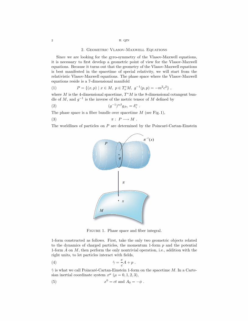
The phase space is a fiber bundle over spacetime M (see Fig. 1),

(3) π : P −→M .

The worldlines of particles on P are determined by the Poincare-Cartan-Einstein

x

M

q

P

π

xπ −1( )

Figure 1. Phase space and fiber integral.

1-form constructed as follows. First, take the only two geometric objects relatedto the dynamics of charged particles, the momentum 1-form p and the potential1-form A on M , then perform the only nontrivial operation, i.e., addition with theright units, to let particles interact with fields,

(4) γ =e

cA + p .

γ is what we call Poincare-Cartan-Einstein 1-form on the spacetime M. In a Carte-sian inertial coordinate system xµ (µ = 0, 1, 2, 3),

(5) x0 = ct and A0 = −φ .

A SHORT INTRODUCTION TO GENERAL GYROKINETIC THEORY 3

The Poincare-Cartan-Einstein 1-form on the phase space P is obtained by pullingback γ,

(6) γ = π∗γ .

Particles’ dynamics is determined by Hamilton’s equation

(7) iτdγ = 0 ,

where τ is a vector field, whose integrals are particle’s worldlines on P .Very elegantly, the Poincare-Cartan-Einstein 1-form γ also gives the necessary

“volume form” needed for the fundamental “velocity integrals” in kinetic theory.Define the Liouville 6-form ω on the 7D phase space P as

(8) ω = − 13!m3

dγ ∧ dγ ∧ dγ .We take the viewpoint that the “velocity integrals” in kinetic theory are geomet-rically fiber integrals [26] defined as follow. For x ∈ M, and q ∈ π−1(x) ⊂ P (seeFig. 1), consider the form

(9) ωx(q)(u1, u2, u3)[v1, v2, v3] ≡ ω(q)(u1, u2, u3, v1, v2, v3) ,

where

ui ∈ Tq [π−1(x)], vi ∈ TxM, Tqπ(vi) = vi, vi ∈ TqP , (i = 1, 2, 3).

Actually, vi is not unique because in general Tqπ is not injective. However, ωx(q) iswell defined because according to the submersion theorem,

(10) Ker(Tqπ) = Tq [π−1(x)] .

Therefore, ωx(q) is a 3-form on π−1(x), valued in 3-forms on M. The 3-form flux onM corresponding to a distribution function f : P −→ R is the result of integrationof fωx over the fiber π−1(x) at x,

(11) j(x) =∫

π−1(x)

fωx .

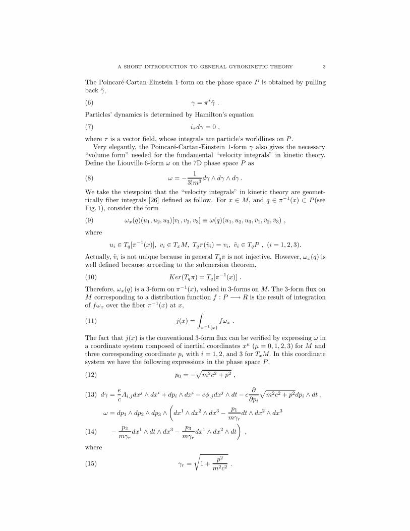
The fact that j(x) is the conventional 3-form flux can be verified by expressing ω ina coordinate system composed of inertial coordinates xµ (µ = 0, 1, 2, 3) for M andthree corresponding coordinate pi with i = 1, 2, and 3 for TxM. In this coordinatesystem we have the following expressions in the phase space P ,

(12) p0 = −√m2c2 + p2 ,

dγ =e

cAi,jdx

j ∧ dxi + dpi ∧ dxi − eφ,jdxj ∧ dt− c

∂

∂pi

√m2c2 + p2dpi ∧ dt ,(13)

ω = dp1 ∧ dp2 ∧ dp3 ∧(dx1 ∧ dx2 ∧ dx3 − p1

mγrdt ∧ dx2 ∧ dx3

− p2

mγrdx1 ∧ dt ∧ dx3 − p3

mγrdx1 ∧ dx2 ∧ dt

),(14)

where

(15) γr =

√1 +

p2

m2c2.

4 H. QIN

The Maxwell equations are

(16) d ∗ dA = 4πe∫

π−1(x)

fωx ,

where ∗α is the Hodge-dual of α on spacetime M. Overall, the Vlasov-Maxwellequations on the 7D phase space P can be geometrically written as

(17) df(v) = 0, ivdγ = 0 , and d ∗ dA = 4πe∫

π−1(x)

fωx .

3. Noether’s Theorem, Symmetries, Kruskal Ring, and LieCoordinate Perturbation

Noether’s theorem links symmetries and invariants. Here, we cast the theoremin the form of forms. Define a symmetry vector field η (infinite small generator) ofγ to be a vector field that satisfies

(18) Lηγ = ds

for some s : P −→ R, where Lη is the Lie derivative. η generates a 1-parametersymmetry group for γ. Using Cartan’s magic formula, we have

(19) d(γ · η) + iηdγ = ds .

For the vector field τ of a worldline,

(20) d(γ · η) · τ = ds · τ ,which implies that γ · η − s is an invariant.

In the present study, we will only consider the non-relativistic case in an inertialcoordinate system for M with x0 = ct. In addition, we chose three correspondingcoordinate pi (i = 1, 2, 3) as the fiber coordinates for P at x with

(21) p0 = −√m2c2 + p2 = −mc − 1

2p2

mc+O

[(p

mc)4

].

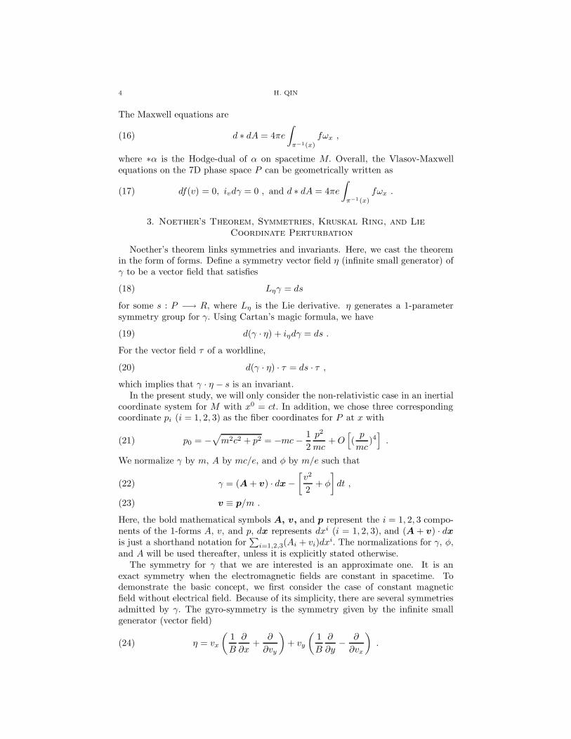
We normalize γ by m, A by mc/e, and φ by m/e such that

γ = (A + v) · dx −[v2

2+ φ

]dt ,(22)

v ≡ p/m .(23)

Here, the bold mathematical symbols A, v, and p represent the i = 1, 2, 3 compo-nents of the 1-forms A, v, and p, dx represents dxi (i = 1, 2, 3), and (A + v) · dxis just a shorthand notation for

∑i=1,2,3(Ai + vi)dxi. The normalizations for γ, φ,

and A will be used thereafter, unless it is explicitly stated otherwise.The symmetry for γ that we are interested is an approximate one. It is an

exact symmetry when the electromagnetic fields are constant in spacetime. Todemonstrate the basic concept, we first consider the case of constant magneticfield without electrical field. Because of its simplicity, there are several symmetriesadmitted by γ. The gyro-symmetry is the symmetry given by the infinite smallgenerator (vector field)

(24) η = vx

(1B

∂

∂x+

∂

∂vy

)+ vy

(1B

∂

∂y− ∂

∂vx

).


Applying Noether’s theorem, we can verify that the corresponding invariant is themagnetic moment

(25) µ =v2

x + v2y

2B.

The gyro-symmetry η has a rather complicated expression in the Cartesian coordi-nates (x, y, vx, vy). A new coordinate will be constructed such that η is a coordinatebase

(26) η =∂

∂θ,

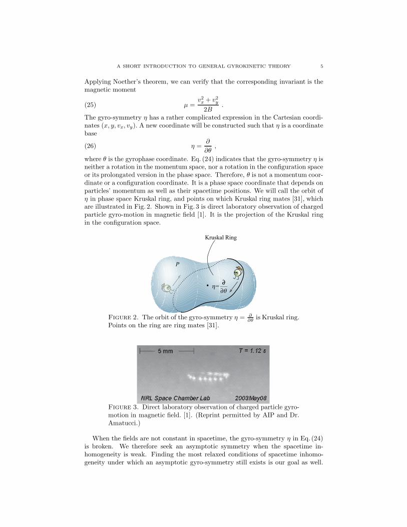
where θ is the gyrophase coordinate. Eq. (24) indicates that the gyro-symmetry η isneither a rotation in the momentum space, nor a rotation in the configuration spaceor its prolongated version in the phase space. Therefore, θ is not a momentum coor-dinate or a configuration coordinate. It is a phase space coordinate that depends onparticles’ momentum as well as their spacetime positions. We will call the orbit ofη in phase space Kruskal ring, and points on which Kruskal ring mates [31], whichare illustrated in Fig. 2. Shown in Fig. 3 is direct laboratory observation of chargedparticle gyro-motion in magnetic field [1]. It is the projection of the Kruskal ringin the configuration space.

P

η= ∂∂∂θ

Kruskal Ring

Figure 2. The orbit of the gyro-symmetry η = ∂∂θ

is Kruskal ring.Points on the ring are ring mates [31].

Figure 3. Direct laboratory observation of charged particle gyro-motion in magnetic field. [1]. (Reprint permitted by AIP and Dr.Amatucci.)

When the fields are not constant in spacetime, the gyro-symmetry η in Eq. (24)is broken. We therefore seek an asymptotic symmetry when the spacetime in-homogeneity is weak. Finding the most relaxed conditions of spacetime inhomo-geneity under which an asymptotic gyro-symmetry still exists is our goal as well.

6 H. QIN

The strategy to achieve our objectives has two steps. (i) Construct a non-fibered,non-canonical phase space coordinate system Z = (X , u, w, θ) such that γ can beexpanded into an asymptotic series

(27) γ = γ0 + γ1 + γ2 + ... ,

where γ1 ∼ εγ0, γ2 ∼ εγ1 , and ε 1. Z is the called the zeroth order gyrocentercoordinate. In addition, γ0 admits the gyro-symmetry η = ∂/∂θ, but γ1 does notnecessarily; (ii) Introduce a coordinate perturbation transformation such that inthe new coordinates Z = (X, u, w, θ), γ1 admits the gyro-symmetry η = ∂/∂θ. Infact, we will seek a stronger symmetry condition

∂γ/∂θ = 0 ,

which is sufficient for η = ∂/∂θ to satisfy Eq. (18). Z is the called the first ordergyrocenter coordinate. The small parameter ε measures the weakness of spacetimeinhomogeneity of the fields. The coordinate perturbation transformation procedureindicates that the most relaxed conditions for the existence of an asymptotic gyro-symmetry is

E ≡ Es + El, B ≡ Bs + Bl,(28)

El ∼ v × Bl

c, Es ∼ ε

v × Bl

c, Bs ∼ ε Bl ,(29) (

|ρ| ∇El

El,

1ΩEl

∂El

∂t

)∼

(|ρ| ∇B

l

Bl,

1ΩBl

∂Bl

∂t

)∼ ε ,(30) (

|ρ| ∇Es

Es,

1ΩEs

∂Es

∂t

)∼

(|ρ| ∇B

s

Bs,

1ΩBs

∂Bs

∂t

)∼ 1 ,(31)

where the fields were split into two parts. (El,Bl) are the large amplitude partswith long spacetime scale length comparable to the spacetime gyroradius ρ =(ρ, 1/Ω), and (Es,Bs) are the small amplitude parts with spacetime scale lengthsmaller than the spacetime gyroradius.

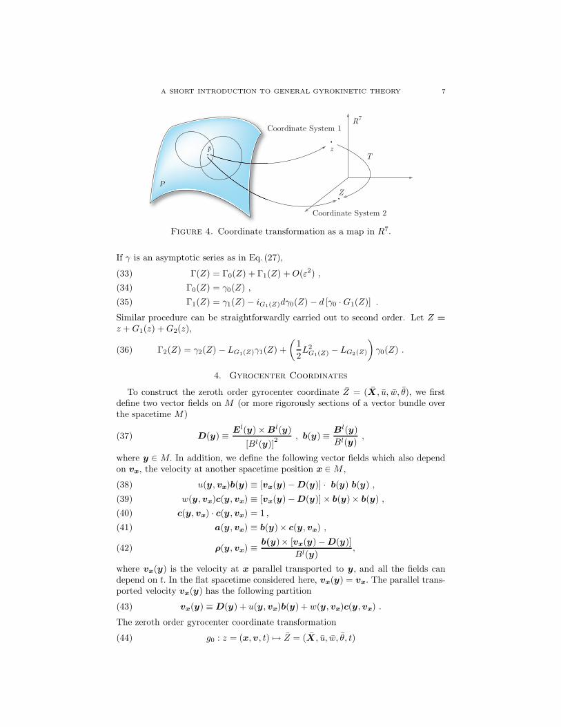
The coordinate perturbation method we adopt belongs to the class of pertur-bation techniques generally referred as Lie perturbation method [3, 6, 7, 37]. Acoordinate transformation for the 7D phase space P can be locally represented bya map between two subsets of the R7 space, T : z −→ Z = T (z). As illustrated inFig. 4, for the same point p in phase space, there could be more than one coordinatesystems (patches). The correspondence between two different coordinate systemsfor the same point in phase space is the coordinate transformation. In the presentstudy, we assume a coordinate transformation can be represented by a single mapalmost everywhere. The subset of phase space which can not be covered by thesingle map has zero measure and does not contribute to the fiber integrals.

To see how γ is transformed by T , let Z = z +G1(z) and G1(z) ∼ ε,

Γ(Z) = γ(z) = γ [Z −G1(z)] = γ[Z −G1(Z) +O(ε2)

]= γ(Z) − LG1(Z)γ(Z) +O(ε2)

= γ(Z) − iG1(Z)dγ(Z) − d [γ ·G1(Z)] +O(ε2) .(32)


P

p z

Z

R

T

7

CoorC diinate System 1

Coordinate System 2

Figure 4. Coordinate transformation as a map in R7.

If γ is an asymptotic series as in Eq. (27),

Γ(Z) = Γ0(Z) + Γ1(Z) +O(ε2) ,(33)

Γ0(Z) = γ0(Z) ,(34)

Γ1(Z) = γ1(Z) − iG1(Z)dγ0(Z) − d [γ0 ·G1(Z)] .(35)

Similar procedure can be straightforwardly carried out to second order. Let Z =z +G1(z) +G2(z),

(36) Γ2(Z) = γ2(Z) − LG1(Z)γ1(Z) +(

12L2

G1(Z) − LG2(Z)

)γ0(Z) .

4. Gyrocenter Coordinates

To construct the zeroth order gyrocenter coordinate Z = (X , u, w, θ), we firstdefine two vector fields on M (or more rigorously sections of a vector bundle overthe spacetime M)

(37) D(y) ≡ El(y) × Bl(y)

[Bl(y)]2, b(y) ≡ Bl(y)

Bl(y),

where y ∈ M. In addition, we define the following vector fields which also dependon vx, the velocity at another spacetime position x ∈ M ,

u(y, vx)b(y) ≡ [vx(y) − D(y)] · b(y) b(y) ,(38)

w(y, vx)c(y, vx) ≡ [vx(y) − D(y)] × b(y)× b(y) ,(39)

c(y, vx) · c(y, vx) = 1 ,(40)

a(y, vx) ≡ b(y)× c(y, vx) ,(41)

ρ(y, vx) ≡ b(y)× [vx(y) − D(y)]Bl(y)

,(42)

where vx(y) is the velocity at x parallel transported to y, and all the fields candepend on t. In the flat spacetime considered here, vx(y) = vx. The parallel trans-ported velocity vx(y) has the following partition

(43) vx(y) ≡ D(y) + u(y, vx)b(y) + w(y, vx)c(y, vx) .

The zeroth order gyrocenter coordinate transformation

(44) g0 : z = (x, v, t) → Z = (X , u, w, θ, t)

8 H. QIN

is defined by

x ≡ X + ρ(X , v) ,(45)

u ≡ u(X, v) ,(46)

w ≡ w(X, v) ,(47)

sin θ ≡ −c(X) · e1(X) ,(48)

t ≡ t ,(49)

where e1(X) is an arbitrary unit vector field in the perpendicular direction, and itcan depend on t as well. Consequently,

(50) v = D(X) + ub(X) + wc(X) .

Substituting Eqs. (45)–(50) into Eq. (22), and expanding terms using the orderingEqs. (28)-(31), we have

γ = γ0 + γ1 + O(ε2) ,

(51)

γ0 =[Al(X, t) + ub(X , t) + D(X , t)

] · dX +w2

2Bl(X, t)dθ

−[u2 + w2 +D(X , t)2

2+ φl(X , t)

]dt ,(52)

γ1 =[w

Bl∇a ·

(ub +

wc

2

)+

12ρ · ∇Bl × ρ − w

Bl∇D · a + As(X + ρ)

]· dX

+[− w3

2Bl3a · ∇Bl · b +

w2

BlAs(X + ρ) · c

]dθ+

[1Bl

As(X + ρ) · a]dw

−[φs(X + ρ) + ρ · ∂D

∂t− 1

2ρ · ∇El · ρ −

(ub +

wc

2

)· wBl

∂a

∂t

]dt .(53)

Here, every field is evaluated at Z and can depend on t, and exact terms of theform dα for some α : P → R have been discarded because their insignificance inHamilton’s equation (7). Computation needed in deriving the above equations isindeed involving. It can be easily verified that ∂γ0/∂θ = 0, but ∂γ1/∂θ = 0. Asdiscussed before, we now introduce a coordinate perturbation to the zeroth ordergyrocenter coordinates Z,

(54) Z = g1(Z) = Z +G1(Z) ,

such that ∂γ1/∂θ = 0 in the first order gyrocenter coordinates Z = (X, u, w, θ).Considering the fact that an arbitrary exact term of the form dα can be added toγ1, we have

(55) γ1(Z) = γ1(Z) − iG1(Z)dγ0(Z) + dS1(Z) ,


which, with Gt = 0, expands into

γ1(Z) =[G1X × Bl −G1ub + ∇S1 +

w

Bl∇a ·

(ub +

wc

2

)+

12ρ · ∇Bl × ρ

− w


]· dX +

[G1X · b +

∂S1

∂u

]du+

[w

BlG1θ +

∂S1

∂w+

+1Bl

As(X + ρ) · a]dw +

[− w

BlG1w +

∂S1

∂θ− w3

2Bl3a · ∇Bl · b

+w

BlAs(X + ρ) · c

]dθ+

[− El · G1X + uG1u +wG1w +

∂S1

∂t− φs(X + ρ)

−ρ · ∂D∂t

+12ρ ·∇El · ρ +

(ub +

wc

2

)· wBl

∂a

∂t

]dt .

(56)

In Eq. (56), every field is evaluated at Z and can depend on t. Extensive calculationsare needed to solve for G1 and S1 from the requirement that ∂γ1/∂θ = 0. We listedthe results without giving the details of the derivation,

G1X = −∂S1

∂u+

w2

2Bl3aa · ∇Bl +

wu

Bl2(∇a · b) × b − w

Bl2(∇D · a) × b

+∇S1 + As(X + ρ)

Bl× b(57)

G1u =w2

2Bl2a · ∇Bl · c +

wu

Blb · ∇a · b − w

Blb · ∇D · a

− b · [∇S1 + As(X + ρ)] ,(58)

G1w =Bl

w

∂S1

∂θ− w2

2Bl2a · ∇Bl · b + c · As(X + ρ) ,(59)

G1θ = −Bl

w

∂S1

∂w+

1w

a · As(X + ρ) .(60)

The determining equation for S1 is

∂S1

∂t+

(El

⊥ × b

Bl+ ub

)· ∇S1 + El

‖∂S1

∂u+Bl ∂S1

∂θ= El

⊥ ·[w2

2Bl3aa · ∇Bl

+wu

Bl2(∇a · b) × b − w

Bl2(∇D · a) × b

]− w2u

2Bl2∇Bl : ca

−wu2

Blb · ∇a · b +

wu

Blb · ∇D · a +

w3

2Bl2a · ∇Bl · b

+w

Bla · ∂D

∂t+ ψs − w2

2Bl2∇El : aa +

uw

Bla · ∂b

∂t.(61)

10 H. QIN

The G1 and S1 in Eqs. (57)-(61) remove the θ-dependence in γ1 , i.e.,

γ (Z) = γ0(Z) + γ1(Z) ,(62)

γ0 =[Al(X, t) + ub(X, t) + D(X, t)

] · dX +w2

2Bl(X, t)dθ

−[u2 +w2 +D(X, t)2

2+ φl(X, t)

]dt ,(63)

γ1(Z) = − w2

2BlR · dX −H1dt ,(64)

H1 = El⊥ · w2

2Bl3∇Bl +

w2u

4Blb · ∇ × b + 〈ψs〉

− w2

4Bl2

(∇ · El − bb : ∇El) − w2

2BlR0 ,(65)

R ≡ ∇c · a , R0 ≡ −∂c∂t

· a ,(66)

ψs ≡ φs(X + ρ) − El⊥ × b

Bl· As(X + ρ) −wc · As(X + ρ) ,(67)

〈α〉 ≡ 12π

∫ 2π

0

αdθ , α ≡ α− 〈α〉 .(68)

Even though Eqs. (57)-(68) are displayed without derivation, it may be necessaryto demonstrate the basic procedures of the derivation. For this purpose, we willoutline here the derivation of the X⊥ and w components of G1 in γ (z) . Let

γ1X(Z) =[G1X × Bl −G1ub + ∇S1 +

w

Bl∇a ·

(ub +

wc

2

)+

12ρ · ∇Bl × ρ

− w


].(69)

We look at the following partition of γ1X(Z) · dX,

(70) γ1X(Z) · dX = b · γ1X(Z)b · dX + γ1X(Z) × b × b · dX .

For the first term in the right hand side of Eq. (70)

b · γ1X(Z) = −G1u + b · ∇S1 + b · As(X + ρ) − w

Blb · ∇D · a

+12

(ρ · ∇Bl × ρ

) · b +w

Bl∇a ·

(ub +

wc

2

)· b .(71)

Choosing G1u to be the form displayed in Eq. (58), we are left with the followingexpression

(72) b · γ1X(Z)b · dX =(− w2

2BlR · b

)b · dX .

Similarly, for the second term in the right hand side of Eq. (70)

γ1X(Z) × b = −G1X⊥Bl + b × ∇S1 − b × As(X + ρ) +w

Blb × ∇D · a

+12ρ

(ρ ·∇Bl

)+w

Bl∇a ·

(ub +

wc

2

)× b .(73)


Choosing G1X⊥ to be the perpendicular component part of the result displayed inEq. (57), we are left with

(74) γ1X(Z) × b × b · dX =(− w2

2BlR⊥

)· dX .

Combining Eqs. (72) and (74), we obtain the first term on the right hand side ofEq. (64). The rest of the derivation for Eqs. (57)-(68) can be carried out in similarprocedures.

A particle’s worldline is given by a vector field τ on phase space P which satisfies

(75) iτdγ = 0 .

The conventional gyrocenter motion equation can be obtained through

(76)dX

dt=τXτt

,du

dt=τuτt

,dw

dt=τwτt

,dθ

dt=τθτt.

After some calculation, we obtain the following explicit expressions up to order εfor gyrocenter dynamics,

dX

dt=

B†

b · B† (u +µ

2b · ∇ × b) − b × E†

b · B† ,(77)

du

dt=

B† · E†

B† · b ,(78)

dθ

dt= Bl + R · dX

dt− R0 +

El · ∇Bl

Bl2+u

2b · ∇ × b

+∂

∂µ〈ψs〉 − 1

2Bl

[∇ · El − bb : ∇El]

,(79)

dµ

dt= 0 , µ ≡ w2

2Bl,(80)

B† ≡ ∇ × [Al(X, t) + ub(X, t) + D(X, t)

],(81)

E† ≡ El − ∇[µBl +

D2

2+ 〈ψs〉

]− u

∂b

∂t− ∂D

∂t.(82)

The modified fields B† and E† can be viewed as those generated by a modifiedpotential A† = (φ†, A†),

φ†(X, t) ≡ φl(X, t) + µBl(X, t) +D(X, t)2

2+ 〈ψs(X, t)〉 ,(83)

A†(X, t) ≡ Al(X, t) + ub(X, t) + D(X, t) ,(84)

B† = ∇ × A†, E† = −∇φ† − ∂A†

∂t.(85)

In Eq. (80), the conserved magnetic momentum µ is constructed asymptoticallywhen the spacetime inhomogeneities are weak. Recently, the concept of adiabaticinvariant has been extended to cases with strong spatial inhomogeneities for mag-netic field [20, 61].

5. Gyrocenter Gauge and Gyro-Gauge

An important fact is that the requirement ∂γ1/∂θ = 0 does not uniquely deter-mine the coordinate perturbation G and the gauge function S, and therefore thefirst order gyrocenter coordinates. There are freedoms in defining the zeroth order

12 H. QIN

gyrocenter coordinates as well. For example, in Ref. [38], the following definitionof the zeroth order gyrocenter coordinates are used

x ≡ X + ρ(X , v) ,(86)

u ≡ u(x, v) ,(87)

w ≡ w(x, v) ,(88)

sin θ ≡ −c(x) · e1(x) ,(89)

t ≡ t .(90)

This choice results in more terms in the expression for γ1. We will call the freedomsin selecting the gyrocenter coordinates gyro-center gauges. In Eq. (66), R andR0 are θ-independent, even though a and c are θ-dependent. Let R = (R0,R),X = (t,X), and ∇ = (−∂/∂t,∇). The γ in Eq. (62) is invariant under the followinggroup of transformation

R −→ R′ + ∇δ(X) ,(91)

θ −→ θ′ + δ(X) .(92)

Apparently, this is a gauge group associated how the gyrophase θ is measured orhow Kruskal ring mates are labeled. Naturally, an appropriate name for this gaugewould be gyro-gauge. The R components of gyro-gauge group were first rigorouslyderived in Ref. [39]. Without R, γ will not be invariant under the gyro-gauge grouptransformation.

6. Pullback Transformation

Even though the γ in Eq. (62) is gyro-gauge invariant, it does not need to be.Different gyro-center gauges can be chosen such that γ is not gyro-gauge invariant.The gyrocenter coordinate system constructed is just a useful coordinate systemfor physics, but not the physics itself. It can depend on the gauges (freedoms) wechoose, as long as it is useful. Gyrocenter coordinate system and the gyrokineticequation are not the total of physics under investigation. What is gauge invariantis the system of gyrokinetic equation and the gyrokinetic Maxwell equations. Thekey element which makes this gyrokinetic system gauge invariant is the pullbacktransformation associated with the gyrocenter coordinate system. Without thisvital element, a number of prominent physics features, such as the presence of thecompressional Alfven wave and a proper description of the gyrokinetic equilibrium,cannot be readily recovered.

Kinetic theory deals with particle distribution function f, which is a functiondefined on the phase space P , f : P → R. As discussed in Sec. 2, the familiar den-sity and momentum velocity integrals needed for Maxwell’s equations are the fiberintegrals j(x) =

∫π−1(x)

fωx at x, which returns a 3-form flux. A coordinate system(x, v) for P is fibered if x are the coordinates for the base, i.e., the spacetime M . Ingyrokinetic theory, however, the useful gyrocenter coordinate system is non-fiberedbecause X are not coordinates for spacetime. The gyrocenter transformation g :z −→ Z is a non-fibered coordinate transformation. No matter which coordinatesystem is used, non-fibered or fibered, the moment integrals are still defined onthe fiber π−1(x) at each x, and j(x) should be invariant under general non-fiberedcoordinate transformations. For the new non-fibered coordinate system Z to beuseful, it is necessary to know the construction of j(x) in it. To be specific, the


current scenario is that the distribution function f is known in the transformednon-fibered coordinate system Z as F (Z). Given F (Z), we need to pull back thedistribution function F (Z) into f(z),

j(x) =∫

π−1(x)

g∗ [F (Z)]ωx ,(93)

g∗ [F (Z)] = F (g(z)) = f(z) .(94)

Considering the asymptotic nature of the construction of the gyrocenter transfor-mation g,

(95) g = g1g0 , g0 : z −→ Z , g1 : Z −→ Z ,

we write

f(z) = g∗F (Z) = g∗0 g∗1 F (Z) = g∗0F

[g1(Z)

]= g∗0

[F (Z) +G · ∇F (Z) +O(ε2)

]= F [g0(z)] +G [g0(z)] · ∇F [g0(z)] +O(ε2) .(96)

7. General Gyrokinetic Vlasov-Maxwell Equations

After constructing the gyrocenter coordinates and the corresponding pullbacktransformation, we are ready to cast the coordinate independent (geometric) Vlasov-Maxwell equations (17) in the gyrocenter coordinates to obtain the general gyroki-netic Vlasov-Maxwell equations. The gyrokinetic Vlasov equation is simply theVlasov equation df(τ ) = 0 in the gyrocenter coordinates Z, which is explicitly

(97)dZj

dt

∂F

∂Zj= 0 , (0 ≤ j ≤ 6) .

Because

(98)∂

∂θ

(dZ

dt

)= 0 ,

the gyrokinetic equation can be easily split into two parts

F = 〈F 〉 + F ,(99)

∂ 〈F 〉∂t

+dX

dt·∇X 〈F 〉 +

du

dt

∂ 〈F 〉∂u

= 0 ,(100)

∂F

∂t+dX

dt· ∇X F +

du

dt

∂F

∂u+dθ

dt

∂F

∂θ= 0 ,(101)

where dX/dt, du/dt, and dθ/dt are given by Eqs. (77)-(79). It is necessary tocomplete the kinetic equations for F with Maxwell’s equation. With the pullbacktransformation (96), the gyrokinetic Maxwell’s equation can be written as

(102) d ∗ dA = 4π∫

π−1(x)

[(F g0) + (G g0) · ∇ (F g0)]ωx .

We emphasize that Eq. (102) is not a new equation which contains different physicsthan the original Maxwell’s equation with moment integral. The more appropriatename for this equation should be “Maxwell’s equation with moment integral (fiberintegral) in the gyrocenter coordinates”.

14 H. QIN

The gyrophase dependent F can be decoupled from the system. Letting F = 0,Eqs. (100) and (102) form a close system for 〈F 〉 and A. We note that F = 0does not imply that f = 0. f becomes gyrophase dependent through the pullbacktransformation (96) andG. Indeed, f andG contain significant amount of importantphysics, which will be demonstrated in the next two sections.

The spirit of the general gyrokinetic theory is to decouple the gyro-phase dy-namics from the rest of particle dynamics by finding the gyro-symmetry, whichis fundamentally different from the conventional gyrokinetic concept of “averagingout” the “fast gyro-motion”. This objective is accomplished by asymptotically con-structing a good coordinate system, which is of course a nontrivial task [16, 17, 40](see Fig. 5). Indeed, it is almost impossible without the Lie coordinate perturba-tion method enabled by the geometric nature of the phase space dynamics. Wedeveloped the gyrokinetic Vlasov-Maxwell equations not as a new set of equations,but rather as the Vlasov-Maxwell equations in the gyrocenter coordinates. Sincethe general gyrokinetic system developed is geometrically the same as the Vlasov-Maxwell equations, all the coordinate independent properties of the Vlasov-Maxwellequations, such as energy conservation, momentum conservation and Liouville vol-ume conservation, are automatically carried over to the general gyrokinetic system.

Figure 5. Quest of useful coordinates [40]. (Peanuts by CharlesSchulz. Reprint permitted by UFS, Inc.)

8. Application: Spitzer Paradox

Now, we turn to the applications of the gyrokinetic theory developed. The firstapplication is related to how to describe plasma equilibrium using the gyrokinetictheory. Spitzer first noticed the obvious differences between the currents describedby the fluid equations and the guiding center motion [53,54]. There are two aspectsof these obvious differences in an equilibrium plasma without flow and electric field.First, the perpendicular current given by the fluid model is the diamagnetic currentb×∇p/B, which is not in the guiding center drift motion. On the other hand, the


curvature drift and the gradient drift for the guiding center motion are not foundin the fluid results. This puzzle, first posed and discussed by Spitzer, is what wecall the Spitzer paradox. To resolve it, we must explain, qualitatively as well asquantitatively, how the diamagnetic current is microscopically generated, and whathappens to the macroscopic counterparts of the curvature drift and the gradientdrift. Here, we will only discuss the first part of the puzzle — how the diamagneticcurrent is generated microscopically. A detailed study of the puzzle and otherrelevant topics can be found in Ref. [50].

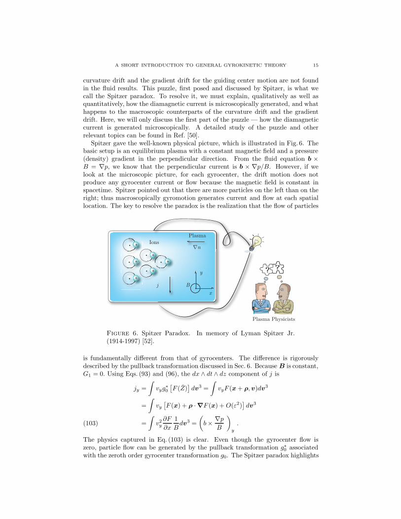
Spitzer gave the well-known physical picture, which is illustrated in Fig. 6. Thebasic setup is an equilibrium plasma with a constant magnetic field and a pressure(density) gradient in the perpendicular direction. From the fluid equation b ×B = ∇p, we know that the perpendicular current is b × ∇p/B. However, if welook at the microscopic picture, for each gyrocenter, the drift motion does notproduce any gyrocenter current or flow because the magnetic field is constant inspacetime. Spitzer pointed out that there are more particles on the left than on theright; thus macroscopically gyromotion generates current and flow at each spatiallocation. The key to resolve the paradox is the realization that the flow of particles

PlasmaIons

Plasma Physicists

j Bx

y

n∇

??

Figure 6. Spitzer Paradox. In memory of Lyman Spitzer Jr.(1914-1997) [52].

is fundamentally different from that of gyrocenters. The difference is rigorouslydescribed by the pullback transformation discussed in Sec. 6. Because B is constant,G1 = 0. Using Eqs. (93) and (96), the dx ∧ dt∧ dz component of j is

jy =∫vyg

∗0

[F (Z)

]dv3 =

∫vyF (x + ρ, v)dv3

=∫vy

[F (x) + ρ ·∇F (x) + O(ε2)

]dv3

=∫v2

y

∂F

∂x

1Bdv3 =

(b× ∇p

B

)y

.(103)

The physics captured in Eq. (103) is clear. Even though the gyrocenter flow iszero, particle flow can be generated by the pullback transformation g∗0 associatedwith the zeroth order gyrocenter transformation g0. The Spitzer paradox highlights

16 H. QIN

the “seeming conflict” between the theory of gyromotion and the fluid equations,two most fundamental concepts in plasma physics, and emphasizes the importantphysics content in the pullback transformation.

9. Application: Bernstein Wave and Compressional Alfven Wave

As examples of applications of the gyrokinetic theory developed to plasma waves,we derive the dispersion relations for the Bernstein wave and the compressionalAlfven wave in this section. A detailed derivation of the complete dispersion relationfor plasma waves with arbitrary wavelength and frequency using the gyrokinetictheory can be found in Ref. [46].

For the Bernstein wave, we consider an electrostatic wave propagating perpen-dicularly in a homogeneous magnetized plasma. Let Bl = Bez = Ωez, El = 0,As = 0, k = kex, and

(104) φs ∼ φ exp (ikx− iωt) .

Linearizing the gyrokinetic equation for F = F0 + F1, we have

(105)dF1

dt=∂F1

∂t+ ub · ∇F = −b · ∇ 〈φ〉 ∂F0

∂u.

Assuming the equilibrium distribution function F0 to be Maxwellian

(106) F0 =n0

(2πT/m)3/2exp

( −v2

2T/m

),

the solution for the linear gyrokinetic equation is degenerate because k‖ ≡ b ·k = 0,

(107) F1 = − 1T/m

F0

−k‖uω − k‖u

〈φ〉 = 0 .

The only physics content is found in the pull-back of the perturbed density, whichrequires expressing the gauge function S1 in terms of the perturbed fields. Theequation for S1 is

(108) Ω∂S1

∂θ+∂S1

∂t= φ(X + ρ) = [ eρ·∇ − J0(

ρ · ∇i

)]φ(X) .

Using the identity

(109) exp(λ cos θ) =∞∑

n=−∞In(λ) exp(inθ) ,

we can easily solve Eq. (108) for S1,

(110) S1 =1

ΩiωJ0φ+

1Ω

∞∑n=−∞

In(iρk)i(n− ω)

e inθ φ .


where ω = ω/Ω. Since F1 = 0, the density response (i.e., the dx∧dt∧dz componentof the 3-form flux in spacetime) comes only from S1 in the pull-back transformation.

n1 =∫g∗0

[F1(Z) +G1 ·∇F0(Z) + O(ε2)

]dv3(111)

=∫

e−ρ·∇G1 ·∇F0(z)dv3 + O(ε2)

=∫

e−ρ·∇ Ωw

∂S1

∂θ

∂F0

∂wdv3 +O(ε2)

=∫

−e ρ·∇ F0

T/m

∞∑n=−∞

nIn(iρk)(n− ω)

e inθ φ(x) d3v + O(ε2) .

Using the facts that

(112)∫ 2π

0

e i(m + n)ξ dξ = δm,−n2π ,

we have(113)

n1 =2π

(2πT )3/2

∫ −n0φ

T/mexp(−

v2‖ + v2

⊥2T/m

)∞∑

n=−∞

nI−n(−iρk)In(iρk)(n − ω)

v⊥dv‖dv⊥ .

Carrying out the algebra with the help of some identities related to the Besselfunctions, we obtain

(114) n1 = n0φ

T/m

∞∑n=1

2n2

(ω

Ω)2 − n2

exp(− k2T

Ω2m)In(

k2T

Ω2m) .

Finally, the Poisson equation (in unnormalized units)

(115) −∇2φ =∑spec

4πen1

gives the dispersion relation of the Bernstein wave

(116) 1 =∑spec

4πn0e2

Tk2

∞∑n=1

2n2

(ω

Ω)2 − n2

exp(− k2T

Ω2m)In(

k2T

Ω2m) .

For low frequency and long wavelength modes, the leading order n1 in Eq. (114) is

n1 = −n0k2φ

Ω2.

Historically, this term has been referred as “the polarization drift term in the Pois-son equation”. It has played an important role in the development of gyrokineticparticle simulation methods [5,11,13,14,19,21,23,33,34,42,57]. However, its deriva-tion were almost always heuristic. Using the general gyrokinetic theory developedhere, this term is rigorously recovered as a special case of the general pullbacktransformation. In an inhomogeneous equilibrium, it is generalized into [47]

(117) n1 = ∇ ·(n0

Ω2∇φ

).

18 H. QIN

Let’s rewrite the Poisson equation for the current case as,

∇ · (εE⊥) = 0 ,(118)

ε = 1 +∑spec

4πn0e2

Ω2m.(119)

Here ε can be viewed as the dielectric constant of the plasma in the perpendiculardirection. This point of view can be justified by the following alternative derivationof Eq. (119). Because

(120) x = X + ρ + G1X ,

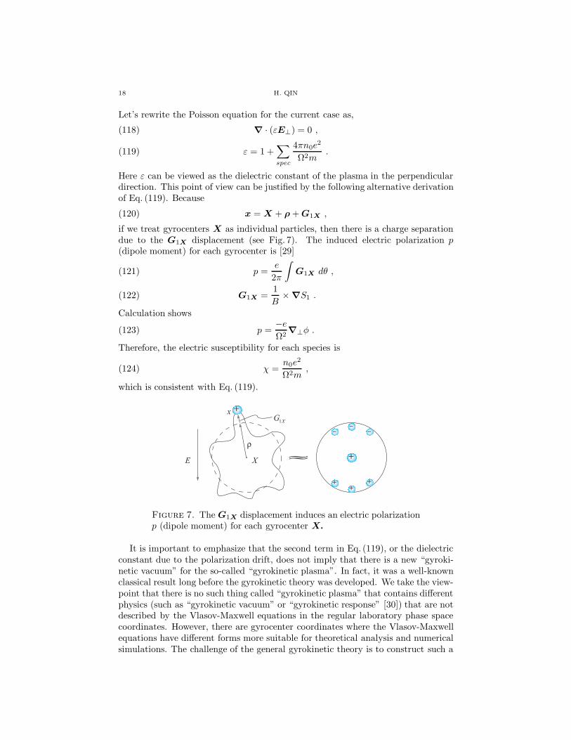
if we treat gyrocenters X as individual particles, then there is a charge separationdue to the G1X displacement (see Fig. 7). The induced electric polarization p(dipole moment) for each gyrocenter is [29]

p =e

2π

∫G1X dθ ,(121)

G1X =1B

× ∇S1 .(122)

Calculation shows

(123) p =−eΩ2

∇⊥φ .

Therefore, the electric susceptibility for each species is

(124) χ =n0e

2

Ω2m,

which is consistent with Eq. (119).

+

+

++

+

-- -

E X

x1XG

ρ≈

Figure 7. The G1X displacement induces an electric polarizationp (dipole moment) for each gyrocenter X.

It is important to emphasize that the second term in Eq. (119), or the dielectricconstant due to the polarization drift, does not imply that there is a new “gyroki-netic vacuum” for the so-called “gyrokinetic plasma”. In fact, it was a well-knownclassical result long before the gyrokinetic theory was developed. We take the view-point that there is no such thing called “gyrokinetic plasma” that contains differentphysics (such as “gyrokinetic vacuum” or “gyrokinetic response” [30]) that are notdescribed by the Vlasov-Maxwell equations in the regular laboratory phase spacecoordinates. However, there are gyrocenter coordinates where the Vlasov-Maxwellequations have different forms more suitable for theoretical analysis and numericalsimulations. The challenge of the general gyrokinetic theory is to construct such a


useful coordinate system and associated pull-back transformation without losing oradding any physics content to the Vlasov-Maxwell equations. Indeed, the dielectricconstant in Eq. (119) is just a limiting case of the most general classical dielectricconstant tensor for magnetized plasmas [55], which has been recovered exactly fromthe general gyrokinetic theory with the most general pullback transformation [46].

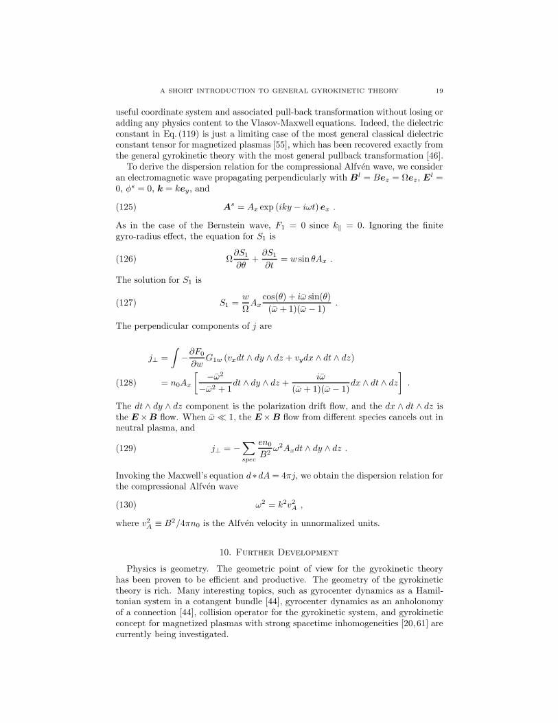
To derive the dispersion relation for the compressional Alfven wave, we consideran electromagnetic wave propagating perpendicularly with Bl = Bez = Ωez, El =0, φs = 0, k = key, and

(125) As = Ax exp (iky − iωt)ex .

As in the case of the Bernstein wave, F1 = 0 since k‖ = 0. Ignoring the finitegyro-radius effect, the equation for S1 is

(126) Ω∂S1

∂θ+∂S1

∂t= w sin θAx .

The solution for S1 is

(127) S1 =w

ΩAx

cos(θ) + iω sin(θ)(ω + 1)(ω − 1)

.

The perpendicular components of j are

j⊥ =∫

−∂F0

∂wG1w (vxdt ∧ dy ∧ dz + vydx ∧ dt ∧ dz)

= n0Ax

[ −ω2

−ω2 + 1dt ∧ dy ∧ dz +

iω

(ω + 1)(ω − 1)dx∧ dt ∧ dz

].(128)

The dt ∧ dy ∧ dz component is the polarization drift flow, and the dx ∧ dt ∧ dz isthe E ×B flow. When ω 1, the E×B flow from different species cancels out inneutral plasma, and

(129) j⊥ = −∑spec

en0

B2ω2Axdt ∧ dy ∧ dz .

Invoking the Maxwell’s equation d ∗dA = 4πj, we obtain the dispersion relation forthe compressional Alfven wave

(130) ω2 = k2v2A ,

where v2A ≡ B2/4πn0 is the Alfven velocity in unnormalized units.

10. Further Development

Physics is geometry. The geometric point of view for the gyrokinetic theoryhas been proven to be efficient and productive. The geometry of the gyrokinetictheory is rich. Many interesting topics, such as gyrocenter dynamics as a Hamil-tonian system in a cotangent bundle [44], gyrocenter dynamics as an anholonomyof a connection [44], collision operator for the gyrokinetic system, and gyrokineticconcept for magnetized plasmas with strong spacetime inhomogeneities [20, 61] arecurrently being investigated.

20 H. QIN

Acknowledgment

I sincerely thank Prof. William M. Tang and Prof. Ronald C. Davidson for theircontinuous support. In the last ten years, I have learned a lot on this subject frommy teachers and colleagues, for which I am grateful. Especially, I would like tothank J. R. Cary, P. J. Channell, L. Chen, Y. Chen, B. I. Cohen, R. H. Cohen,R. C. Davidson, A. M. Dimits, W. D. Dorland, N. J. Fisch, A. Friedman, G. W.Hammet, T. S. Hahm, J. A. Krommes, M. Kruskal, R. M. Kulsrud, G-L. Kuang,W. W. Lee, J-G. Li, Z. Lin, W. M. Nevins, G. Rewoldt, E. Sonnendrucker, H.Sugama, W. M. Tang, X. Tang, Y-X. Wan, T-S. F. Wang, S. J. Wang, and X. Xufor inspirations and fruitful discussions. Finally, I thank Prof. Thierry Passot, Prof.Pierre-Louis Sulem, and Prof. Catherine Sulem for the invitation to give lectureson this subject at the Fields Institute.

References

[1] W. E. Amatucci, D. N. Walker, G. Gatling, and E. E. Scime, Direct observation of mi-

croparticle gyromotion in a magnetized direct current glow discharge dusty plasma, Physicsof Plasmas 11 (2004), no. 5, 2097–2105.

[2] T. M. Antonsen and B. Lane, Kinetic-equations for low-frequency instabilities in inhomoge-neous plasmas, Physics of Fluids 23 (1980), no. 6, 1205–1214.

[3] V. I. Arnold, Mathematical methods of classicalmechanics, second ed., pp. 240–241, Springer-Verlag, New York, 1989.

[4] A. Brizard, Nonlinear gyrokinetic Maxwell-Vlasov equations using magnetic coordinates,Journal of Plasma Physics 41 (1989), no. 6, 541–559.

[5] J. Candy and R. E. Waltz, Anomalous transport scaling in the DIII-D tokamak matched bysupercomputer simulation, Physical Review Letters 91 (2003), no. 4, 045001.

[6] J. R. Cary, Lie transform perturbation-theory for Hamiltonian-systems, Physics Reports-Review Section of Physics Letters 79 (1981), no. 2, 129–159.

[7] J. R. Cary and R. G. Littlejohn, Noncanonical Hamiltonian-mechanics and its application

to magnetic-field line flow, Annals of Physics 151 (1983), no. 1, 1–34.[8] P. J. Catto, Linearized gyro-kinetics, Plasma Physics and Controlled Fusion 20 (1978), no. 7,

719–722.[9] P. J. Catto, W. M. Tang, and D. E. Baldwin, Generalized gyrokinetics, Plasma Physics and

Controlled Fusion 23 (1981), no. 7, 639–650.[10] L. Chen and S. T. Tsai, Electrostatic-waves in general magnetic-field configurations, Physics

of Fluids 26 (1983), no. 1, 141–145.[11] Y. Chen and S. E. Parker, A delta-f particle method for gyrokinetic simulations with kinetic

electrons and electromagnetic perturbations, Journal of Computational Physics 189 (2003),no. 2, 463–475.

[12] G. F. Chew, M. L. Goldberger, and F. E. Low, The Boltzmann equation and the one-fluidhydromagnetic equations in the absence of particle collisions, Proceedings of the Royal Society

of London Series A-Mathematical and Physical Sciences 236 (1956), no. 1204, 112–118.[13] B. I. Cohen, T. A. Brengle, D. B. Conley, and R. P. Freis, An orbit averaged particle code,

Journal of Computational Physics 38 (1980), no. 1, 45–63.[14] B. I. Cohen, T. J. Williams, A. M. Dimits, and J. A. Byers, Gyrokinetic simulations of EXB

velocity-shear effects on ion-temperature-gradient modes, Physics of Fluids B-Plasma Physics5 (1993), no. 8, 2967–2980.

[15] R. C. Davidson, Invariant of higher-order Chew-Goldberger-Low theory, Physics of Fluids 10(1967), no. 3, 669–670.

[16] R. C. Davidson and H. Qin, Physics of intense charged particle beams in high energy accel-erators, pp. 301–352, World Scientific, Singapore, 2001.

[17] R. C. Davidson, H. Qin, and P. J. Channell, Periodically-focused solutions to the nonlinearVlasov-Maxwell equations for intense charged particle beams, Physics Letters a 258 (1999),

no. 4-6, 297–304.


[18] A. M. Dimits, L. L. Lodestro, and D. H. E. Dubin, Gyroaveraged equations for both the

gyrokinetic and drift-kinetic regimes, Physics of Fluids B-Plasma Physics 4 (1992), no. 1,274–277.

[19] A. M. Dimits, T. J. Williams, J. A. Byers, and B. I. Cohen, Scalings of ion-temperature-gradient-driven anomalous transport in tokamaks, Physical Review Letters 77 (1996), no. 1,

71–74.[20] I. Y. Dodin and N. J. Fisch, Motion of charged particles near magnetic-field discontinuities,

Physical Review E 6401 (2001), no. 1, 016405.[21] W. Dorland, F. Jenko, M. Kotschenreuther, and B. N. Rogers, Electron temperature gradient

turbulence, Physical Review Letters 85 (2000), no. 26, 5579–5582.[22] D. H. E. Dubin, J. A. Krommes, C. Oberman, and W. W. Lee, Non-linear gyrokinetic equa-

tions, Physics of Fluids 26 (1983), no. 12, 3524–3535.[23] A. Friedman, A. B. Langdon, and B. I. Cohen, A direct method for implicit particle-in-cell

simulation, Comments Plasma Phys. Controlled Fusion 6 (1981), 225–236.[24] E. A. Frieman and L. Chen, Non-linear gyrokinetic equations for low-frequency

electromagnetic-waves in general plasma equilibria, Physics of Fluids 25 (1982), no. 3, 502–508.

[25] E. A. Frieman, R. C. Davidson, and B. Langdon, Higher-order corrections to chew-goldberger-low theory, Physics of Fluids 9 (1966), no. 8, 1475–1482.

[26] W. Greub, S. Halperin, and R. Vanstone, Connections and curvature and cohomology, vol. II,pp. 242–243, Academic Press, New York, 1973.

[27] T. S. Hahm, Nonlinear gyrokinetic equations for tokamak microturbulence, Physics of Fluids31 (1988), no. 9, 2670–2673.

[28] T. S. Hahm, W. W. Lee, and A. Brizard, Nonlinear gyrokinetic theory for finite-beta plasmas,Physics of Fluids 31 (1988), no. 7, 1940–1948.

[29] J. D. Jackson, Classical electrodynamics, pp. 137–146, John Wiley & Sons, New York, 1975.[30] J. A. Krommes, Dielectric response and thermal fluctuations in gyrokinetic plasma, Physics

of Fluids B-Plasma Physics 5 (1993), no. 4, 1066–1100.[31] M. Kruskal, Asymptotic theory of Hamiltonian and other systems with all solutions nearly

periodic, Journal of Mathematical Physics 3 (1962), no. 4, 806–828.[32] R.M. Kulsrud, Adiabatic invairant of the harmonic oscillator, Physical Review 106 (1957),

no. 2, 205–207.[33] W. W. Lee, Gyrokinetic approach in particle simulation, Physics of Fluids 26 (1983), no. 2,

556–562.[34] Z. Lin, T. S. Hahm, W. W. Lee, W. M. Tang, and R. B. White, Turbulent transport reduction

by zonal flows: Massively parallel simulations, Science 281 (1998), no. 5384, 1835–1837.[35] R. G. Littlejohn, Guiding center Hamiltonian - new approach, Journal of Mathematical

Physics 20 (1979), no. 12, 2445–2458.[36] , Hamiltonian-formulation of guiding center motion, Physics of Fluids 24 (1981),

no. 9, 1730–1749.[37] , Hamiltonian theory of guiding center bounce motion, Physica Scripta T2 (1982),

119–125.

[38] , Variational-principles of guiding center motion, Journal of Plasma Physics 29(1983), no. 2, 111–125.

[39] , Phase anholonomy in the classical adiabatic motion of charged-particles, PhysicalReview a 38 (1988), no. 12, 6034–6045.

[40] L. Michelotti, Intermediate classical dynamics with applications to beam physics, p. 240, JohnWiley & Sons, New York, 1995.

[41] T. G. Northrop, The adiabatic motion of charged particles, pp. 78–95, John Wiley & Sons,New York, 1963.

[42] S. E. Parker, W. W. Lee, and R. A. Santoro, Gyrokinetic simulation of ion-temperature-gradient-driven turbulence in 3d toroidal geometry, Physical Review Letters 71 (1993), no. 13,

2042–2045.[43] H. Qin, Gyrokinetic theory and computational methods for electromagnetic perturbations in

tokamaks, Ph.D. thesis, Princeton University, Princeton, NJ 08540, 1998.[44] , Differential geometry and gyrokinetic theory, Bulletin of the American Physical

Society (New York), vol. 47, American Physical Society, 2002, p. 295.

22 H. QIN

[45] H. Qin and W. M. Tang, Pullback transformations in gyrokinetic theory, Physics of Plasmas

11 (2004), no. 3, 1052–1063.[46] H. Qin, W. M. Tang, and W. W. Lee, Gyrocenter-gauge kinetic theory, Physics of Plasmas 7

(2000), no. 11, 4433–4445.[47] H. Qin, W. M. Tang, W. W. Lee, and G. Rewoldt, Gyrokinetic perpendicular dynamics,

Physics of Plasmas 6 (1999), no. 5, 1575–1588.[48] H. Qin, W. M. Tang, and G. Rewoldt, Gyrokinetic theory for arbitrary wavelength electro-

magnetic modes in tokamaks, Physics of Plasmas 5 (1998), no. 4, 1035–1049.[49] , Linear gyrokinetic theory for kinetic magnetohydrodynamic eigenmodes in tokamak

plasmas, Physics of Plasmas 6 (1999), no. 6, 2544–2562.[50] H. Qin, W. M. Tang, G. Rewoldt, and W. W. Lee, On the gyrokinetic equilibrium, Physics

of Plasmas 7 (2000), no. 3, 991–1000.[51] P. H. Rutherford and E. A. Frieman, Drift instabilities in general magnetic field configura-

tions, Physics of Fluids 11 (1968), no. 3, 569–585.[52] D. C. Spitzer, 2004, Private communication with Mrs. D. C. Spitzer.

[53] L. Spitzer, Equations of motion for an ideal plasma, Astrophysical Journal 116 (1952), no. 2,299–316.

[54] L. Spitzer, Physics of fully ionized gases, second ed., pp. 30–40, Interscience Publications,New York, 1962.

[55] T. H. Stix, Waves in plasmas, pp. 247–262, American Institute of Physics, New York, 1992.[56] H. Sugama, Gyrokinetic field theory, Physics of Plasmas 7 (2000), no. 2, 466–480.

[57] R. D. Sydora, V. K. Decyk, and J. M. Dawson, Fluctuation-induced heat transport resultsfrom a large global 3D toroidal particle simulation model, Plasma Physics and Controlled

Fusion 38 (1996), no. 12A, A281–A294.[58] W. M. Tang, Introduction to gyrokinetic theory with applications in magnetic confinement

research in plasma physics, Topics in Kinetic Theory (D. Levermore, T. Passot, C. Sulem,and P.L. Sulem, eds.), Fields Institute Communications, American Mathematical Society,

2004, in this volume.[59] J. B. Taylor and R. J. Hastie, Stability of general plasma equilibria .I. formal theory, Plasma

Physics 10 (1968), no. 5, 479–494.[60] S. J. Wang, Canonical Hamiltonian gyrocenter variables and gauge invariant representation

of the gyrokinetic equation, Physical Review E 64 (2001), no. 5, 056404.[61] H. Weitzner and C. Chang, Extensions of adiabatic invariant theory for a charged particle,

Physics of Plasmas 12 (2005), no. 12, 012106.

Princeton Plasma Physics Laboratory, Princeton University, Princeton, NJ 08543,USA

E-mail address : [email protected]

01/18/05

External Distribution Plasma Research Laboratory, Australian National University, Australia Professor I.R. Jones, Flinders University, Australia Professor João Canalle, Instituto de Fisica DEQ/IF - UERJ, Brazil Mr. Gerson O. Ludwig, Instituto Nacional de Pesquisas, Brazil Dr. P.H. Sakanaka, Instituto Fisica, Brazil The Librarian, Culham Science Center, England Mrs. S.A. Hutchinson, JET Library, England Professor M.N. Bussac, Ecole Polytechnique, France Librarian, Max-Planck-Institut für Plasmaphysik, Germany Jolan Moldvai, Reports Library, Hungarian Academy of Sciences, Central Research Institute

for Physics, Hungary Dr. P. Kaw, Institute for Plasma Research, India Ms. P.J. Pathak, Librarian, Institute for Plasma Research, India Professor Sami Cuperman, Plasma Physics Group, Tel Aviv University, Israel Ms. Clelia De Palo, Associazione EURATOM-ENEA, Italy Dr. G. Grosso, Instituto di Fisica del Plasma, Italy Librarian, Naka Fusion Research Establishment, JAERI, Japan Library, Laboratory for Complex Energy Processes, Institute for Advanced Study,

Kyoto University, Japan Research Information Center, National Institute for Fusion Science, Japan Dr. O. Mitarai, Kyushu Tokai University, Japan Dr. Jiangang Li, Institute of Plasma Physics, Chinese Academy of Sciences,

People’s Republic of China Professor Yuping Huo, School of Physical Science and Technology, People’s Republic of China Library, Academia Sinica, Institute of Plasma Physics, People’s Republic of China Librarian, Institute of Physics, Chinese Academy of Sciences, People’s Republic of China Dr. S. Mirnov, TRINITI, Troitsk, Russian Federation, Russia Dr. V.S. Strelkov, Kurchatov Institute, Russian Federation, Russia Professor Peter Lukac, Katedra Fyziky Plazmy MFF UK, Mlynska dolina F-2,

Komenskeho Univerzita, SK-842 15 Bratislava, Slovakia Dr. G.S. Lee, Korea Basic Science Institute, South Korea Dr. Rasulkhozha S. Sharafiddinov, Theoretical Physics Division, Insitute of Nuclear Physics,

Uzbekistan Institute for Plasma Research, University of Maryland, USA Librarian, Fusion Energy Division, Oak Ridge National Laboratory, USA Librarian, Institute of Fusion Studies, University of Texas, USA Librarian, Magnetic Fusion Program, Lawrence Livermore National Laboratory, USA Library, General Atomics, USA Plasma Physics Group, Fusion Energy Research Program, University of California

at San Diego, USA Plasma Physics Library, Columbia University, USA Alkesh Punjabi, Center for Fusion Research and Training, Hampton University, USA Dr. W.M. Stacey, Fusion Research Center, Georgia Institute of Technology, USA Dr. John Willis, U.S. Department of Energy, Office of Fusion Energy Sciences, USA Mr. Paul H. Wright, Indianapolis, Indiana, USA

The Princeton Plasma Physics Laboratory is operatedby Princeton University under contract

with the U.S. Department of Energy.

Information ServicesPrinceton Plasma Physics Laboratory

P.O. Box 451Princeton, NJ 08543

Phone: 609-243-2750Fax: 609-243-2751

e-mail: [email protected] Address: http://www.pppl.gov

Gyrokinetic plasma theory

Science

Transcript of Gyrokinetic plasma theory