Gurobi Optimization - edgestone-it.com · The Gurobi Products Gurobi Solvers Mi dMixed-It P...

Gurobi Optimization

Pushing the Frontiers of Optimization Performance

Agenda

12:00-12:25 Introduction◦ Bob Bixby

12:25-12:50 Accessing Gurobi◦ Greg Glockner12 50 1 25 G bi T h l 12:50-1:25 Gurobi Technology◦ Bob Bixby

1:25-1:40 Break 1:40-2:00 Gurobi Best Practices◦ Greg Glockner

2:00-2:20 Performance 2:20-2:30 The Future◦ Bob Bixby

Question & Answer

2© 2010 Gurobi Optimization18-Jun-10

Gurobi Optimization

Gurobi Optimization, Inc.p , Incorporated July, 2008 Founders: Zonghao Gu, Ed Rothberg, Bob Bixby

Product Releases Version 1.0: May 2009

LP simplex & MIP LP simplex & MIP Version 2.0: October 2009

LP simplex & MIP performance improvementsp p p Version 3.0: April 2010

LP barrier, MIP performance improvements


Company Business Model

Focus on math programming solversp g g◦ Our business is helping our customers succeed with

math programming solutions◦ Provide the best possible support from people whoProvide the best possible support from people who

know math programming Be a flexible partner◦ Licensing models that meet user needs◦ Licensing models that meet user needs◦ Clear, upfront pricing

Be the technology leader◦ Build the best available math programming

technology


The Gurobi Products

Gurobi SolversMi d I t P i◦ Mixed-Integer Programming Deterministic, parallel

◦ Linear Programming Dual and primal simplexAll d d f◦ All standard features

APIs◦ Simple command-line interface◦ Python interactive interfacePython interactive interface◦ C, C++, Java, Python callable libraries◦ All standard modeling languages

Gurobi CloudEC2 offering◦ EC2 offering

Commercial and Academic Licenses◦ Licensing options and pricing available at www.gurobi.com


Gurobi Gurobi Commercial PartnersCommercial Partners

GurobiGurobi NonNon Commercial PartnersCommercial PartnersGurobi Gurobi NonNon--Commercial PartnersCommercial Partners

ParamILS


Expanding the Reach of Optimization


Expanding the Reach of O i i iOptimization Parallel at no extra chargeg◦ Gurobi was the first

Free Trial Licenses◦ Automated download and license generation◦ Automated download and license generation◦ 500 variable by 500 constraint size limit

Academic Program◦ Free single-user licenses for academics Automated download and license generation Bi-weekly validationy

The Gurobi Cloud◦ You only pay for what you use


Free Academic Licenses

Here are the steps:p

Request a Gurobi account Download and install software Generate and download license key Install and validate the license key◦ Does a reverse DNS lookup of origin domain

Must be repeated at least once every 2 weeks◦ Must be repeated at least once every 2 weeks


Expanding the reach of Optimization

Over 1500 free academic licenses issued 50% outside the US 30% appear to be outside the OR community◦ Martin Albrecht, University of London, "I am a grad student in the

Information Security Group (ISG) at Royal Holloway, University of London. I work on algebraic aspects of symmetric cryptology under the supervision of Carlos Cid.”

◦ Shoibal Chakravarty, Energy Group, Princeton University, "Chakravarty is developing a global CO2 emissions attribution profile.”

◦ Tai-Hsuan Wu, EE, U Wisconsin, "His research interests are in the area of computer-aided design and with an emphasis on power aware and high performance design techniques, parallel optimization, and grid computing environments."


What’s New in Gurobi 3.0


New in Gurobi 3.0

Parallel Barrier Optimizer New .NET API Significantly Improved MIP performance◦ Dominance techniques Symmetry checking

◦ Additional and improved cutting planes Submip cuts

◦ New heuristics◦ New heuristics◦ New presolve reductions

Other ◦ Improved memory management in MIP◦ Improved memory management in MIP◦ API for accessing multiple MIP solutions◦ New parameters and more access to parameters Examples: MIPfocus parameter, more access to heuristicsp p ,


Questions?Questions?

Accessing GurobiAccessing Gurobi

Methods to access Gurobi

Command-line executable◦ Simple tool to test model files

Programming interfaces◦ APIs to build and solve models

Modeling systems◦ Wide variety of commercial and free partners◦ Wide variety of commercial and free partners


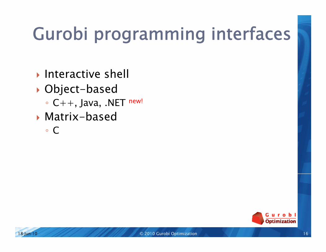
Gurobi programming interfaces

Interactive shell Object-based◦ C++, Java, .NET new!

Matrix-based◦ C


Common structure

Streamlined◦ Gurobi Attributes replace long list of get/set

functions

Fast◦ Lazy updates process model changes in a batch◦ Lazy updates process model changes in a batch

Low memory overhead Low memory overhead


Gurobi interactive shell

A complete programming environmentp p g g◦ Based on Python language◦ Supports all Gurobi algorithms and features

Easily build virtually any optimization applicationapplication◦ Solve a model file◦ Build a model through codeg◦ Solve a sequence of models◦ Import / export with databases


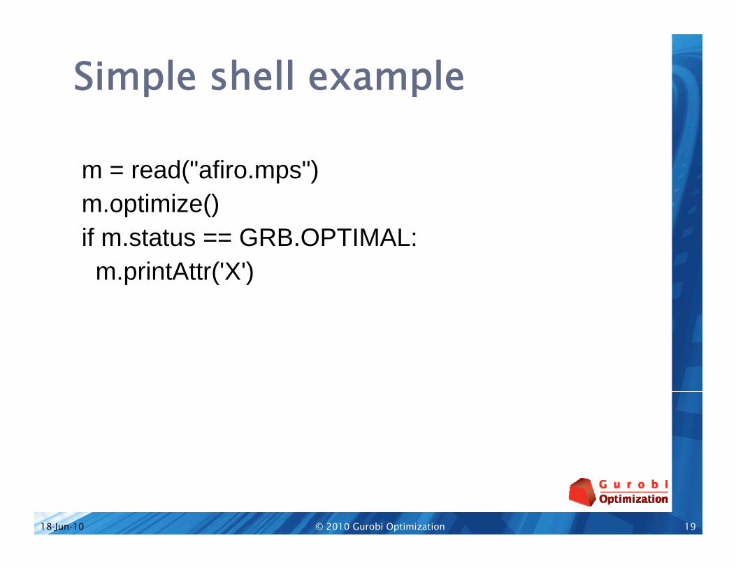
Simple shell example

m = read("afiro.mps")m read( afiro.mps )m.optimize()if m.status == GRB.OPTIMAL:m.printAttr('X')


Simple shell example – 2

m = read("afiro.mps")m read( afiro.mps )m.optimize()if m.status == GRB.OPTIMAL:for i in m.getVars():print i.VarName, i.X, i.RC


Modeling in the shell

# Create a new modelm = Model("mip1")

# Create variables and objective: x + y + 2z# Create variables and objective: x y 2zx = m.addVar(0.0, 1.0, -1.0, GRB.BINARY, "x")y = m.addVar(0.0, 1.0, -1.0, GRB.BINARY, "y")z = m addVar(0 0 1 0 2 0 GRB BINARY "z")z = m.addVar(0.0, 1.0, -2.0, GRB.BINARY, z )

# Integrate new variablesm.update()


Modeling in the shell – 2

# Add constraint: x + 2 y + 3 z <= 4m.addConstr(LinExpr([1.0, 2.0, 3.0], [x, y, z]), GRB.LESS_EQUAL,

4.0, "c0")

# Add constraint: x + y >= 1m.addConstr(LinExpr([1.0, 1.0], [x, y]), GRB.GREATER_EQUAL, 1.0,

"c1")c1 )

# Solve and write solution to filem optimize()m.optimize()m.write("mip1.sol")


Object modeling interfaces

Represent models using objectsp g j◦ Objects for variables◦ Objects for constraintsF i h d i Function methods to create constraints, columns

Similar structure◦ C++, Java, .NET, PythonC++, Java, .NET, Python


Objects in a simple constraint:1x + y ≥ 1

C++ JavaC++model.addConstr(x+y>=1, "c1");

Javaexpr = new GRBLinExpr();expr.addTerm(1.0, x);

ddT (1 0 )expr.addTerm(1.0, y);model.addConstr(expr,

GRB.GREATER_EQUAL, 1.0, "c1");c1 );


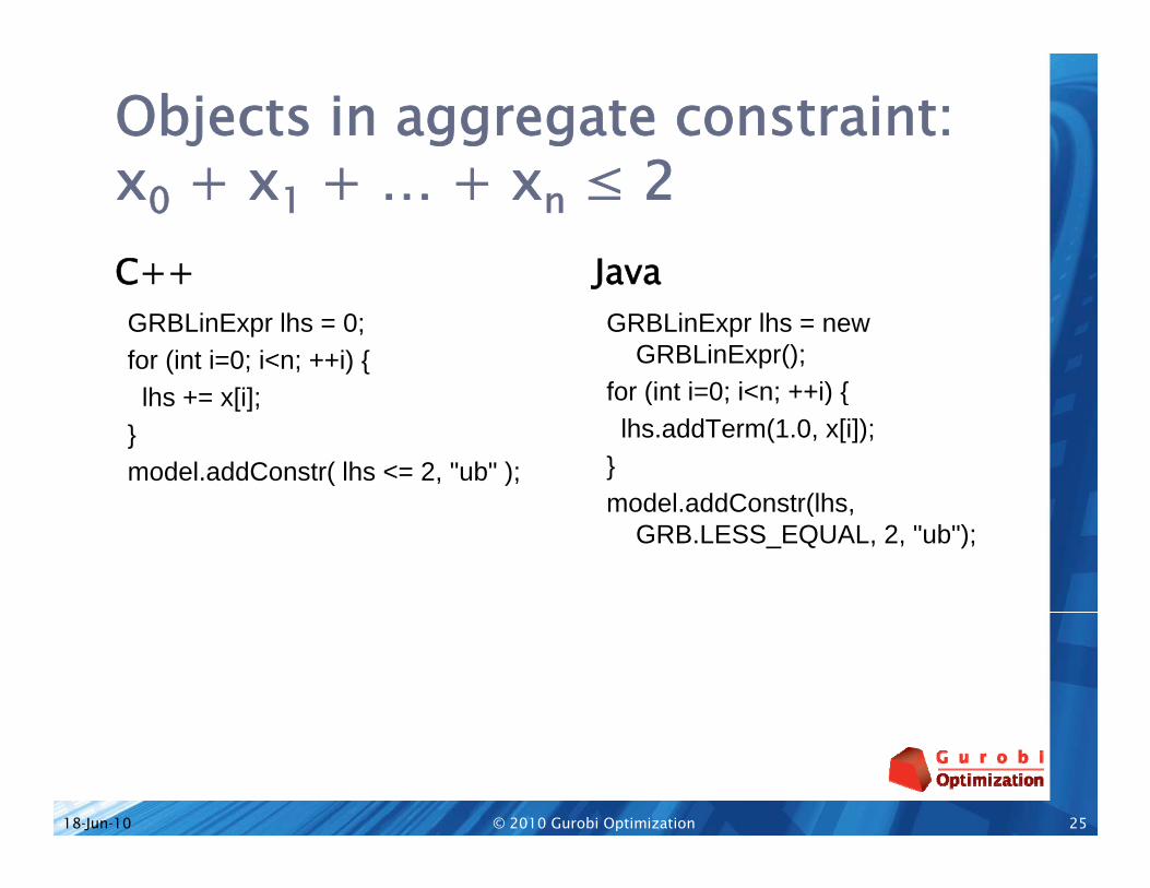
Objects in aggregate constraint:2x0 + x1 + … + xn ≤ 2

C++ JavaC++GRBLinExpr lhs = 0;for (int i=0; i<n; ++i) {lh [i]

JavaGRBLinExpr lhs = new

GRBLinExpr();for (int i=0; i<n; ++i) {lhs += x[i];

}model.addConstr( lhs <= 2, "ub" );

for (int i=0; i<n; ++i) {lhs.addTerm(1.0, x[i]);

}model addConstr(lhsmodel.addConstr(lhs,

GRB.LESS_EQUAL, 2, "ub");


C: Sparse matrix interface

Compressed sparse row formatp p◦ GRBaddconstrs()

Compressed sparse column format◦ GRBaddvars()

St d d f t d b l Standard formats used by many solvers◦ Use simple arrays to represent Matrix coefficients Index positions for these coefficients◦ Virtually no changes required to existing code


Accessing attributes

Object interfacej◦ get/set methods on the objects◦ C++ example

d l (GRB I A N NZ )nz = model.get(GRB_IntAttr_NumNZs);var.set(GRB_DoubleAttr_UB, 1.0);

Matrix interface◦ get/set functions by type (int, double, char, string)◦ C example◦ C example

status = GRBgetintattr(model, "NumNZs", &nz);status = GRBsetdblattrelement(model, "UB", varidx, 1.0);


Role of attributes

Unified system to access model elementsy◦ Attributes work the same across all Gurobi

interfaces – C, C++, Java, .NET, Python

Attributes refer to model elements◦ Access via a basic set of get and set functions Attribute name is specified as a parameter◦ Replaces many functions used by other solvers

Full list in Attributes section of Reference Manual


Selected attributes

The model itself◦ Number of variables, constraints, nonzeros◦ Solve time

S l ti t t ( ti l i f ibl t )◦ Solution status (optimal, infeasible, etc.) Individual variables◦ Solution value upper bound lower boundSolution value, upper bound, lower bound◦ Objective coefficients◦ Type – continuous, binary, general integer, etc.

Individual constraints◦ Values for right-hand side, slack, dual


Gurobi TechnologyGurobi Technology

Gurobi Parallel Barrier Solver

Gurobi Barrier

New deterministic parallel barrier solver in pGurobi 3.0◦ Parallel:

k f h h Makes use of as many cores as your machine has Gurobi license is always a parallel license◦ Deterministic: Same result each time


Gurobi Barrier Features

Barrier solver includes:◦ Parallel sparse Cholesky factorization Dominant computation in barrier Highly tuned factorization kernelsHighly tuned factorization kernels Achieve 80-90% of machine peak performance

◦ Other parallel steps AAT computation AAT computation Sparse matrix reordering, using latest reordering techniques

◦ Multiple central correctionsS hi ti t d d l d f i bl h dli◦ Sophisticated dense column and free variable handling

◦ Crossover algorithm to provide a basic solution


Barrier Is Interesting

When solving an LP from scratch…◦ 267 models that require more than 1s for either dual or

barrier◦ Geomean barrier runtime (including crossover): 1 core: 1.00x 4 cores:0.70x

Not so interesting when you have advanced start information…◦ For a set of 240 MIP models that require 1-10s to solve:For a set of 240 MIP models that require 1 10s to solve: 5.3x slower if you use barrier to reoptimize the node

relaxations


Barrier Is Getting More Interesting

Barrier can make effective use of parallelism p(unlike simplex)◦ Cholesky factorization, AA’ computation, triangular

solve, etc.solve, etc.◦ Explosion of parallelism in recent years: Multi-core chips SSE instruction set SSE instruction set◦ More coming: Multiply-accumulate instruction in next generation

x86 chipsx86 chips 2x peak floating-point performance

Yet more cores


Barrier and Simplex –J i d h HiJoined at the Hip Even when solving an LP from scratch, barrier g ,

relies heavily on simplex◦ Simplex much more numerically stable

h l ll h ll l b h Much less numerically challenging to solve Ax=b than ADATx = b

◦ Crossover becomes more important as barrier gets faster For models that require > 1s: 1 core: crossover is 10% of total barrier runtime1 core: crossover is 10% of total barrier runtime 4 cores: crossover is 15% of total barrier runtime Crossover more than 50% of runtime for 24% of models


Improving Crossover

Significant improvements in stability of g p ycrossover in Gurobi 3.0◦ Losses of feasibility less common and less

t t hicatastrophic Developed new options for building initial

crossover basiscrossover basis◦ Can sometimes avoid lengthy crossover steps

With improvements in barrier performance, improving crossover will become more and more important


MIP IMIP Improvements


Improving a MIP Solver

Improvements can be plotted on two axes:p p

SpeedupBig speedups onBig speedups on Big speedups onlots of models

g speedups oa few models

Modest speedupson lots of models

Generality


New Ideas

Speedup

Nine out of tenideas end up here

Experience

GeneralityExperiencegenerally keeps you away from here


Gurobi 3.0

S dSpeedup Symmetry

SubMIP cutsNew presolve red.

BarrierNetwork cuts

SubMIP cuts

Cut tuning

Generality


MIP D i iMIP Domination


MIP Domination

MIP domination◦ A feasible solution X is (strictly) dominated by a

feasible solution Y, if Y has objective value as good as (better than) X.( )◦ Suppose for any feasible solution X with Xj > a,

there exists another feasible solution Y with Yj <= a such that Y dominates X. Then we need only yconsider xj <= a.

Use of domination information Use of domination information◦ Reduce or simplify MIP models◦ Avoid unnecessary search


Domination Techniques

Presolve reductions Dominated nodes detection Symmetry breaking


A Simple Presolve Reduction

ConsiderMin 5 x1 + 4 x2 + 11 x3 + 4 y1 + 2 y2s.t. x1 + x2 + 3 x3 + y1 + y2 <= 7

2 x1 + 2 x2 + 2 x3 + y1 <= 101 2 3 1 2 > 0x1, x2, x3, y1, y2 >= 0

x1, x2, x3 are integers

ll l l Parallel columns◦ x1 and x2 are parallel and x1 is dominated because of its

objective coefficient


Dual Presolve Reductions

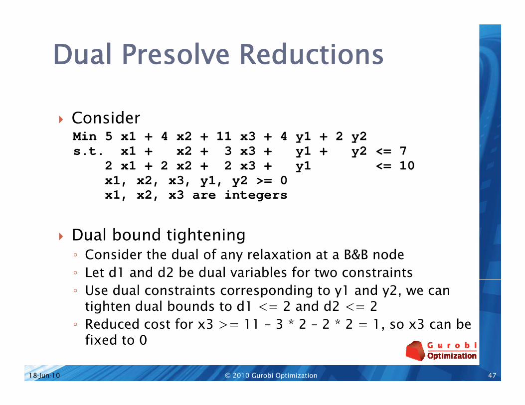
ConsiderMin 5 x1 + 4 x2 + 11 x3 + 4 y1 + 2 y2s.t. x1 + x2 + 3 x3 + y1 + y2 <= 7

2 x1 + 2 x2 + 2 x3 + y1 <= 101 2 3 1 2 > 0x1, x2, x3, y1, y2 >= 0

x1, x2, x3 are integers

l b d h Dual bound tightening◦ Consider the dual of any relaxation at a B&B node◦ Let d1 and d2 be dual variables for two constraints ◦ Use dual constraints corresponding to y1 and y2, we can

tighten dual bounds to d1 <= 2 and d2 <= 2◦ Reduced cost for x3 >= 11 – 3 * 2 – 2 * 2 = 1, so x3 can be ,

fixed to 0


Another Presolve Reduction

Consider◦ a x + b y = c◦ x, y are integer variables◦ a, b and c are integers, a > 1◦ Assume gcd(a b) 1◦ Assume gcd(a,b) = 1 Otherwise a Euclidean reduction is possible

◦ Observation: Then x(mod b) and y(mod a) are constants. Reduction Reduction◦ Substitute y = a z + d (d is easy to compute).◦ z has a smaller search space than y

General application General application◦ Can easily be extended to general “all integer”

constraints.


Dominated Nodes

0-1 knapsack examplep pMin 5 x1 + 6 x2 + 7 x3 + 9 x4 + sum wj xj

3 x1 + 4 x2 + 5 x3 + 6 x4 + sum aj xj <= b

At a node At a node◦ (x1, x2, x3, x4) = (1, 0, 0, 1)

Let◦ cost(x1, x2, x3, x4) = 5 x1 + 6 x2 + 7 x3 + 9 x4◦ a(x1, x2, x3, x4) = 3 x1 + 4 x2 + 5 x3 + 6 x4

Then ◦ cost(0,1,1,0) < cost(1,0,0,1) ◦ a(0,1,1,0)= a(1,0,0,1)◦ The node is dominatedThe node is dominated


Dominated Nodes

Consider a general MIPgMin eTx + fTy + gTzs.t. A x + B y + C z <= b

A, B and C are matricesA, B and C are matricesx, y, z are variable vectors x are binarysome y z are integer or binarysome y, z are integer or binary

At a node◦ x is fixed to (branched to) x*

h “f d ” b d◦ y represent the extra “freedom” beyond x Note just for simplicity, we assume◦ All constraints are inequalitiesq◦ Variables x are binary


Dominated Nodes

Lets(y*) = Min eTx + fTy

s.t. A x + B y <= A x* + B y*x are binaryx are binarysome y are integer or binary

If s(y*) < eTx* + fTy* for all y*, then the node is dominateddominated

Two alternatives◦ If |x| is small and y is empty, computing s(.) is often cheap.

However s(.) < eTx* is rare in those cases.◦ With non-empty y, where y has special properties, we can

sometimes solve for s(y*).


Dominated Nodes

Fixed charge sub-networksg◦ Binary variables indicate whether arcs are open◦ x are the binary variables branched to one

S th t f t i l◦ Suppose the support of x contains a cycle. ◦ Then using y defined by this cycle, we can conclude

that the node is dominated.


Symmetry

Definition◦ Given a MIP

Min { cTx | A x <= b, integrality conditions on x}L t◦ Letα: a column permutation of Aβ: a row permutation of Aβ pPC: a set of all column permutationsPR: a set of all row permutationsA t i d fi d◦ A symmetry group is defined asG = {α in PC | there exists β in PR, such that

(β ,α)(A) = A, α(c) = c and β(b) = b}(β , )( ) , ( ) β( ) }


Exploiting Symmetry

Find symmetry groupy y g p

Use to improve MIP search


Symmetry

Finding the Symmetry groupg y y g p◦ Considerable published work on graph

automorphismsSeveral computer programs are available e g NAUTY Several computer programs are available, e.g. NAUTY and SAUCY

◦ Easy to translate MIP symmetry problem into graph hi (P 2005)automorphisms (Puget 2005).


Symmetry

Exploit in MIP searchp◦ Several papers over last10 years Adding cuts: Rothberg (2000)

F th t i d M t (2002) Fathom symmetric nodes: Margot (2002) Orbit branching: Ostrowski, Linderoth, Rossi, and

Smriglio (2007).◦ Commercial MIP software Introduced in CPLEX 9 Substantially improved in CPLEX 10Substantially improved in CPLEX 10


Symmetry

Gurobi 3.0◦ Implemented symmetry detection directly using the matrix◦ Apply orbital branching plus several additional ideas◦ 28% of models in our test set have symmetry28% of models in our test set have symmetry◦ Performance is affected on 50% of those with symmetry◦ Many unsolvable models become solvable◦ 25% geometric speedup on the whole set (including those◦ 25% geometric speedup on the whole set (including those

without symmetry)


C i PlCutting Planes


Cutting Planes

New cutting planesg p◦ Network cuts◦ Submip cutsI f i i i Improvement of existing cut routines◦ Aggregation for MIR and flow cover◦ Cut filterCut filter


Network Cut

Finding network structure ◦ Use a simple heuristic to find a set of network rows ◦ Identify associated fixed-charge indicator variables

SeparationSepa at o◦ Sort arcs based on relaxation values◦ Use the order to construct a spanning tree (forest) ◦ RepeatRepeat Remove a non-leaf arc from the spanning tree splits

network into two parts Aggregate each of the two parts Look for violated flow-cover cut

Performance◦ 10% speedup on models with network structure.p p


SUBMIP Cut

Solve submip to generate cutsp g◦ Expensive, not typically applied in default◦ Used in Mipfocus=2 and 3M i id Main idea◦ Rather different from ideas that solve a sub-MIP to

separateseparate◦ Closer to some ideas developed for TSP


Cut Changes Summary

Overall performance improvementp p◦ 20% speedup on our internal model set

Largest effect is on hard models when using fMipfocus = 2 or 3


Gurobi Best PracticesGurobi Best Practices

Performance tuning

Gurobi Optimizer is designed to be fast and p grobust with default parameters

But a few high-level parameters may improve performance, particularly for MIP


General tuning advice

Presolve: controls the level of presolvep-1 Automatic setting (default)0 Off1 Conservative1 Conservative2 Aggressive

M l k d l i l◦ More presolve can make a model easier to solve◦ But presolve can be time-consuming


General tuning advice – 2

Threads: controls number of parallel threadsp◦ More threads may speed up barrier & MIP◦ For MIP, more threads requires more memory

D f lt l b f /◦ Default value: number of cores/processors

◦ Take care if processor supports hyperthreading Ex: Intel Core i7 processors


LP tuning advice

LPMethod: controls algorithm to use for LP or gnode LPs in MIP

0 Primal simplex1 Dual simplex (default)1 Dual simplex (default)2 Barrier – not recommended for MIP

RootMethod: controls whether to use primal, dual or barrier for root LP in MIP◦ Same values as LPMethod above


MIP tuning advice

MIPFocus: Sets the focus of the MIP solver0 Balance good feasibles & optimality (default)1 Focus on finding feasible solutions2 Focus on proving optimality2 Focus on proving optimality3 Focus on moving the best bound

N i G bi O i i 3 0◦ New in Gurobi Optimizer 3.0


MIP tuning advice – 2

Cuts: Global control over the level of cuts-1 Automatic setting (default)0 Off1 Conservative1 Conservative2 Aggressive3 Very aggressive

◦ More cuts can make a model easier to solve◦ But cuts can be time-consumingg◦ Similar settings for individual types of cuts


MIP tuning advice – 3

Heuristics: Controls the amount of time spent pin MIP heuristics

D f l l 0 05◦ Default value: 0.05◦ Larger values produce more and better feasible

solutions◦ But spending more time on heuristics leads to

slower progress on the bound


Pitfalls to avoid

Setting parametersg p

Lazy model updates


Setting parameters

Parameters are set on a Gurobi environment

A Gurobi model has a copy of the Gurobienvironment◦ Each model can use its own set of parameters

But you must set parameters on the environment◦ But you must set parameters on the environment for the model


Parameters example

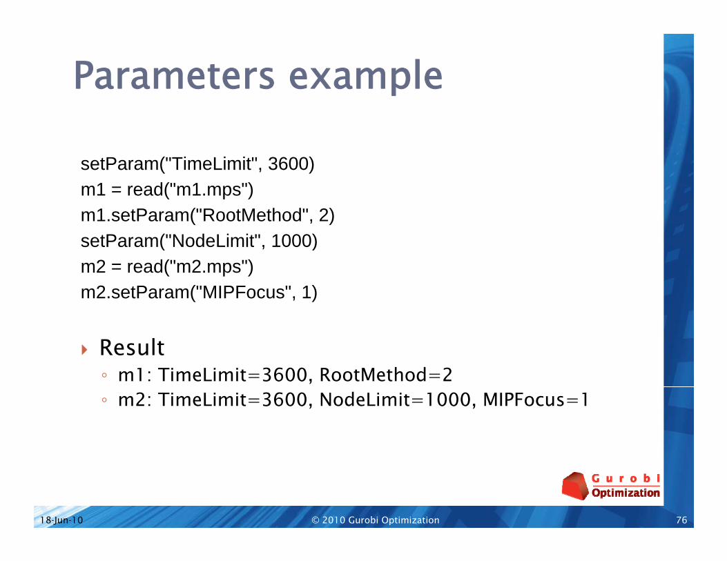
setParam("TimeLimit", 3600)m1 = read("m1.mps")m1.setParam("RootMethod", 2)setParam("NodeLimit", 1000)setParam( NodeLimit , 1000)m2 = read("m2.mps")m2.setParam("MIPFocus", 1)

Result◦ m1: TimeLimit=3600, RootMethod=2◦ m2: TimeLimit=3600, NodeLimit=1000, MIPFocus=1


Lazy updates

Gurobi updates models in batch modep

Must call update() to use model elements◦ Ex: Call update() after creating a variable before

using it in a constraint

Model creation and updates are efficient


PerformancePerformance

B i P fBarrier Performance

LP Performance Benchmarks

Performance test sets:◦ Mittelmann LP test sets: LP problems – barrier w/ crossover and simplex

38 d l 38 models http://plato.asu.edu/ftp/lpcom.html

◦ Our own broader test set: Publicly available models, plus customer models

Test platform:◦ a Linux PC (2 67 GHz Intel Core 2)◦ a Linux-PC (2.67 GHz Intel Core 2)


LP Performance – Public BenchmarkG bi CPLEX 12 1Gurobi vs. CPLEX 12.1

Dual Simplex (Mittelmann Test Set)#Models Speedup Speedup

Gurobi 2.0 Gurobi 3.038 1.3X 1.4X

Barrier w/ Crossover (Mittelmann Test Set)#Models Speedup

Gurobi 3 0Gurobi 3.038 1.9X

◦ Additional interesting comparison:g p 1.40X faster for the barrier step 1.55x faster for the crossover step No, it’s not a contradiction

MIP P fMIP Performance

MIP Performance Benchmarks

Performance test sets:Mitt l ti lit t t t◦ Mittelmann optimality test set: 55 models, varying degrees of difficulty http://plato.asu.edu/ftp/milpc.html

◦ Mittelmann feasibility test set:ff f f 33 models, difficult to find feasible solutions

http://plato.asu.edu/ftp/feas_bench.html◦ Mittelmann infeasibility test set: 11 models, objective is to prove infeasibility http://plato.asu.edu/ftp/infeas.html

◦ Our own broader test set: A set of 647 models that require between 1s and 10000s to solve on

four coresP bli l il bl d l l f d l Publicly available models, plus a few customer models

Test platform:◦ Q9450 (2.66 GHz, quad-core system)


MIP Performance –Gurobi Internal Test Set Gurobi V3.0 vs. V2.0 (P=4)

Gurobi Internal Test Set( )

◦ 2458 total models in test set 1350 solve in < 1 second 794 solve by at least one in < 10000 seconds 314 solved by neither in < 10000 seconds

Ti # M d l S dTime # Models Speedup> 1s 794 1.59x> 10s 521 1 95x> 10s 521 1.95x> 100s 295 2.92x> 1000s 144 6 73x> 1000s 144 6.73x

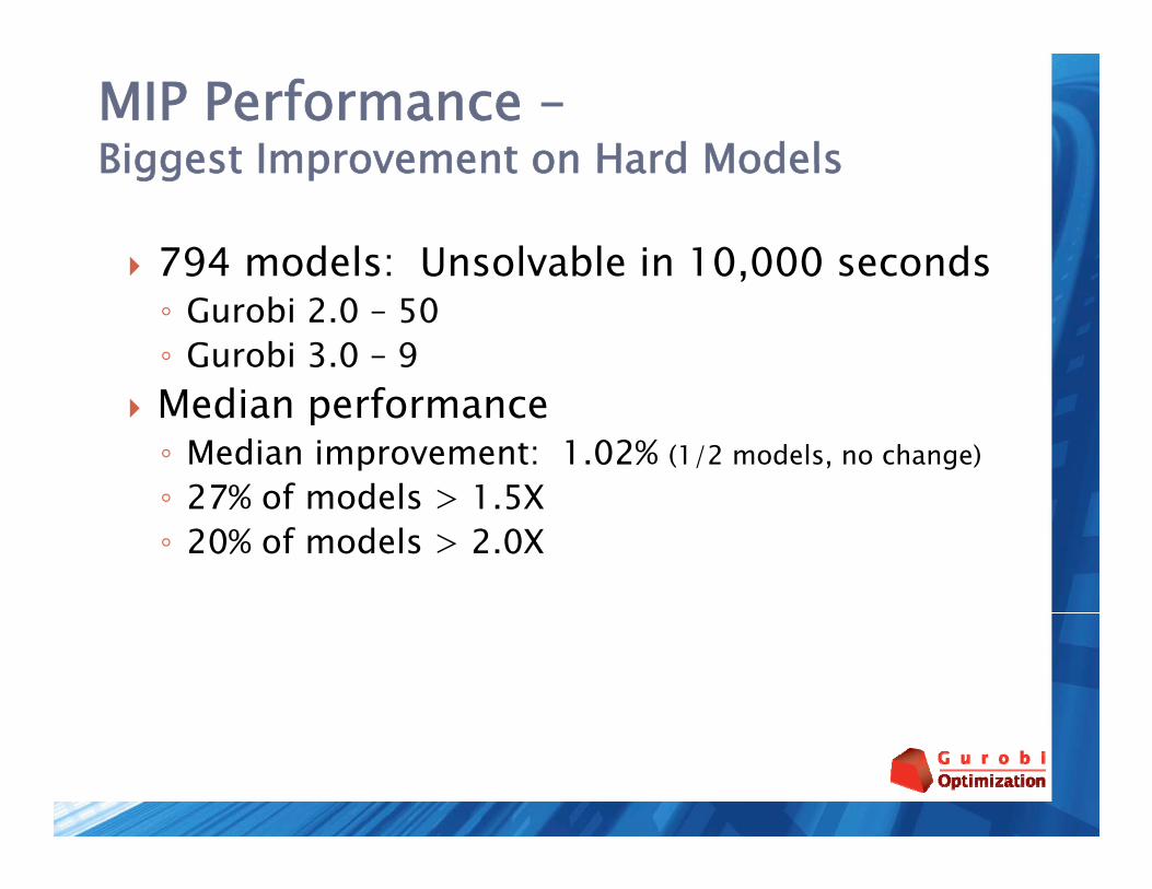
MIP Performance –Biggest Improvement on Hard Models

794 models: Unsolvable in 10,000 seconds

Biggest Improvement on Hard Models

,◦ Gurobi 2.0 – 50◦ Gurobi 3.0 – 9

d f Median performance◦ Median improvement: 1.02% (1/2 models, no change)◦ 27% of models > 1 5X◦ 27% of models > 1.5X ◦ 20% of models > 2.0X

MIP Performance –P bli B h kPublic Benchmarks Gurobi 2.0 vs CPLEX 12.1:

P=1 P=4Optimality 1.56X 1.74XFeasibility 4.22X -Infeasibility - 2.43

G bi 3 0 CPLEX 12 1 Gurobi 3.0 vs CPLEX 12.1:P=1 P=4

Optimality 1 75X 1 87XOptimality 1.75X 1.87XFeasibility 4.76X -Infeasibility - 4.09X


P ll l P fParallel Performance

Parallel Performance (V2.0 data)

Parallel speedups (Gurobi P=1 vs P=4):p p ( )P=4 speedup

>1s 1.54>10s 1.64>100s 1.79

CPLEX reported (for CPLEX 11) 1.36X speedup for P=4 on their broader set for models taking more th 1than 1s


The Future: Performance, P f P fPerformance, Performance

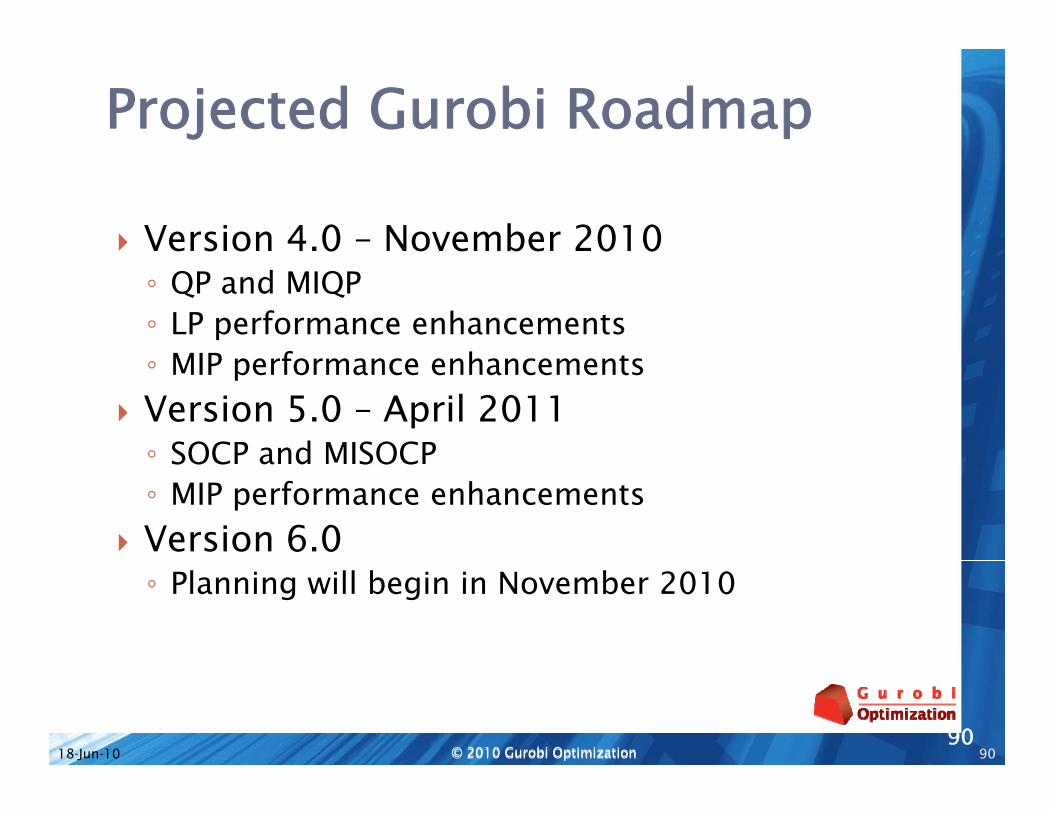
Projected Gurobi Roadmap

Version 4.0 – November 2010◦ QP and MIQP◦ LP performance enhancements

MIP f h t◦ MIP performance enhancements Version 5.0 – April 2011◦ SOCP and MISOCPSOCP and MISOCP◦ MIP performance enhancements

Version 6.0◦ Planning will begin in November 2010


© 2010 Gurobi Optimization

Company Business Model

Focus on math programming solversp g g◦ Our business is helping our customers succeed with

math programming solutions◦ The best possible support from people who knowThe best possible support from people who know

math programming Be a flexible partner◦ Licensing models that meet user needs◦ Licensing models that meet user needs◦ Clear, upfront pricing

Be the technology leader◦ Build the best available math programming

technology


Gurobi Optimization - edgestone-it.com · The Gurobi Products Gurobi Solvers Mi dMixed-It P...

Documents

Transcript of Gurobi Optimization - edgestone-it.com · The Gurobi Products Gurobi Solvers Mi dMixed-It P...