GURJHQ$ WRPkau.diva-portal.org/smash/get/diva2:947133/FULLTEXT01.pdf · First of all I would like...
59
Path Integral for the Hydrogen Atom Solutions in two and three dimensions Vägintegral för Väteatomen Lösningar i två och tre dimensioner Anders Svensson Faculty of Health, Science and Technology Physics, Bachelor Degree Project 15 ECTS Credits Supervisor: Jürgen Fuchs Examiner: Marcus Berg June 2016
-
Upload
nguyennguyet -
Category
Documents
-
view
212 -
download
0
Transcript of GURJHQ$ WRPkau.diva-portal.org/smash/get/diva2:947133/FULLTEXT01.pdf · First of all I would like...
Path Integral for the Hydrogen Atom
Solutions in two and three dimensions
Vägintegral för Väteatomen Lösningar i två och tre dimensioner
Anders Svensson
Faculty of Health, Science and Technology
Physics, Bachelor Degree Project
15 ECTS Credits
Supervisor: Jürgen Fuchs
Examiner: Marcus Berg
June 2016
Abstract
The path integral formulation of quantum mechanics generalizes the action principle of classicalmechanics. The Feynman path integral is, roughly speaking, a sum over all possible paths that a particlecan take between fixed endpoints, where each path contributes to the sum by a phase factor involvingthe action for the path. The resulting sum gives the probability amplitude of propagation betweenthe two endpoints, a quantity called the propagator. Solutions of the Feynman path integral formulaexist, however, only for a small number of simple systems, and modifications need to be made whendealing with more complicated systems involving singular potentials, including the Coulomb potential.We derive a generalized path integral formula, that can be used in these cases, for a quantity calledthe pseudo-propagator from which we obtain the fixed-energy amplitude, related to the propagator by aFourier transform. The new path integral formula is then successfully solved for the Hydrogen atom intwo and three dimensions, and we obtain integral representations for the fixed-energy amplitude.
Sammanfattning
Vagintegral-formuleringen av kvantmekanik generaliserar minsta-verkanprincipen fran klassisk meka-nik. Feynmans vagintegral kan ses som en summa over alla mojliga vagar en partikel kan ta mellan tvagivna andpunkter A och B, dar varje vag bidrar till summan med en fasfaktor innehallande den klas-siska verkan for vagen. Den resulterande summan ger propagatorn, sannolikhetsamplituden att partikelngar fran A till B. Feynmans vagintegral ar dock bara losbar for ett fatal simpla system, och modifika-tioner behover goras nar det galler mer komplexa system vars potentialer innehaller singulariteter, sasomCoulomb–potentialen. Vi harleder en generaliserad vagintegral-formel som kan anvandas i dessa fall, foren pseudo-propagator, fran vilken vi erhaller fix-energi-amplituden som ar relaterad till propagatorn viaen Fourier-transform. Den nya vagintegral-formeln loses sedan med framgang for vateatomen i tva ochtre dimensioner, och vi erhaller integral-representationer for fix-energi-amplituden.

Acknowledgements
First of all I would like to thank my supervisor, Professor Jurgen Fuchs, for the interesting discussionsand for helping me out with all of the hard questions. I would also like to thank my father, for teachingme elementary mathematics and physics in the beginning of my studies, as well as the rest of my familyand friends for their great support over the years. Last, but not least, I must thank all of the greatphysicists including Leonard Susskind, Brian Greene, and Richard Feynman himself, for making me lovephysics and inspiring me to continue on to the next level.

Contents
1 Introduction 1
2 Basic Concepts 32.1 Classical Mechanics . . . . . . . . . . . . . . . . . . . . . . . . . . . . . . . . . . . . . . . . . . 32.2 Quantum Mechanics . . . . . . . . . . . . . . . . . . . . . . . . . . . . . . . . . . . . . . . . . 4
3 Propagators 73.1 The Propagator and its Properties . . . . . . . . . . . . . . . . . . . . . . . . . . . . . . . . . 73.2 The Retarded Propagator and Fixed-Energy Amplitude . . . . . . . . . . . . . . . . . . . . . 9
4 Path Integrals 134.1 The Short-time Propagator . . . . . . . . . . . . . . . . . . . . . . . . . . . . . . . . . . . . . 134.2 The Finite-time Propagator From the Short-time Propagator . . . . . . . . . . . . . . . . . . 144.3 The Phase Space Path Integral . . . . . . . . . . . . . . . . . . . . . . . . . . . . . . . . . . . 144.4 The Configuration Space Path Integral . . . . . . . . . . . . . . . . . . . . . . . . . . . . . . . 16
5 Finding a More Flexible Path Integral Formula 185.1 The Pseudo-propagator . . . . . . . . . . . . . . . . . . . . . . . . . . . . . . . . . . . . . . . 185.2 New Path Integral Formula: Phase Space . . . . . . . . . . . . . . . . . . . . . . . . . . . . . 225.3 New Path Integral Formula: Configuration Space . . . . . . . . . . . . . . . . . . . . . . . . . 23
6 Exact Solution for the Hydrogen Atom 266.1 The Hydrogenic Path Integral in D Dimensions . . . . . . . . . . . . . . . . . . . . . . . . . . 266.2 Solution for the Two-Dimensional H-atom . . . . . . . . . . . . . . . . . . . . . . . . . . . . . 276.3 Solution for the Three-Dimensional H-atom . . . . . . . . . . . . . . . . . . . . . . . . . . . . 32
7 Conclusion 39
A Gaussian Integrals 40
B Exact Solutions for some Simple Path Integrals 43B.1 The Free Particle . . . . . . . . . . . . . . . . . . . . . . . . . . . . . . . . . . . . . . . . . . . 43B.2 The Harmonic Oscillator . . . . . . . . . . . . . . . . . . . . . . . . . . . . . . . . . . . . . . . 45
C Square-root Coordinates for the 3-D H-atom 52

1 Introduction
Developed by Richard Feynman in the 1940s, the path integral formulation of quantum mechanics generalizesthe action principle of classical mechanics. In classical mechanics, extremizing the action functional S[x(t)]determines the unique path x(t) taken by a particle between two endpoints xa,xb. In quantum mechanicsthere is no such path describing the motion of the particle. Instead, the quantum particle has a probabilityamplitude for going from xa to xb. Feynman showed that this probability amplitude is obtained by summingup phase factors exp
[i~S[x(t)]
]over each and every path connecting xa and xb. This sum is called the
Feynman path integral, written as
ˆ xb
xa
D [x(t)] exp
[i
~S[x(t)]
]. (1.1)
This expression is to be viewed as a functional integral. While an ordinary integral´ xb
xadx f(x) sums up
values of a function f(x) over all numbers x from xa to xb, a functional integral´ xb
xaD [x(t)]F [x(t)] sums
up values of a functional F [x(t)] over all functions x(t) with endpoints x(ta) = xa and x(tb) = xb. Moreexplicitly, the Feynman path integral may be expressed in D dimensions as
ˆ xb
xa
D [x(t)] exp
[i
~S[x(t)]
]= limN→∞
( m
2πi~δt
)DN/2 ˆdDxN−1 · · ·
ˆdDx1 exp
[i
~S[x{xi}(t)]
](1.2)
where m is the particle’s mass, δt = (tb − ta)/N and x{x1,...,xN−1}(t) is a piecewise linear path with valuesxk at the times tk = ta + kδt (k = 1, . . . , N − 1) as well as the endpoints xa and xb at the times ta andtb, respectively. The integrals on the right hand side of (1.2) are understood to go over the whole of RD.It is important to understand that the resulting ”sum” is over all possible paths x{xi}(t) taking the values{xa,x1,x2, . . . ,xb} at the times {ta, t1, t2, . . . , tb} – even those that are absurd from a classical viewpoint. Inthe limit N →∞ we have tk − tk−1 → 0, but |xk −xk−1| will in general be large for an arbitrary such path,resulting in a highly discontinuous path. Only a small subset of paths will be continuous and differentiable.
In general, it is hard to give the functional integral (1.1) a precise mathematical meaning. Accordingly,(1.1) should be viewed as a formal expression that needs to be supplemented by a proper prescription onhow to evaluate it. In particular, it is possible to define (1.1) as a sum over the subset of continuouspaths (see Glimm and Jaffe [5], chapter 3). For a standard form of the action, one can then show that thepath integral resulting from this definition coincides with the right-hand side of (1.2) [5]. This means thatthe discontinuous paths do not contribute to the overall sum in the continuum limit. Consequently, whenevaluating the path integral (1.2) one can make approximations such as |xk+1|/|xk| → 1 to first order in δt.
In mathematics, the basic idea of the path integral can be traced back to the Wiener integral, introduced byNorbert Wiener for solving problems dealing with Brownian motion and diffusion. In physics, the idea wasfurther developed by Paul Dirac in his 1933 paper [1], for the use of the Lagrangian in quantum mechanics.Inspired by Dirac’s idea, Feynman worked out the preliminaries in his 1942 doctoral thesis, before developingthe complete formulation in 1948 [1]. The Feynman path integral has since become one of the most prominenttools in quantum mechanics and quantum field theory. Other areas of application include
• quantum statistics, where the quantum mechanical partition function can be written as, or obtainedfrom, a path integral in imaginary time;
• polymer physics, where path integrals are useful for studying the statistical fluctuations of chains ofmolecules, modelled as random chains consisting of N links; and
• financial markets, where the time dependence of prices of assets can be modelled by fluctuating paths.
In physics, path integrals have found their main application in perturbative quantum field theory. In ele-mentary quantum mechanics, however, the formulation has not had as much impact due to the difficulties indealing with the resulting path integrals, with only a few standard problems having been solved analytically.
1

In particular, the path integral for the Hydrogen atom remained unsolved until Duru and Kleinert publishedtheir solution in 1979 [2].
The goal of this thesis is to provide an exact solution of the path integral for the Hydrogen atom, followingthe steps of Duru–Kleinert. Before doing so, we shall develop the necessary preliminaries, including aderivation of the path integral formalism. Moreover, due to the singular nature of the Coulomb potential,the corresponding path integral can be shown to diverge when written down in the original form [4], andhence a new, modified, path integral must be constructed.
In the following Section we begin by reviewing some basic concepts from classical mechanics and quantummechanics. In Section 3 we continue by studying the propagator and its related quantities, including thefixed-energy amplitude, which is related to the propagator by a Fourier transform. We then derive the basicpath integral formulas in phase space and configuration space in Section 4, before deriving more flexibleversions of these in Section 5 that can be applied to problems involving singular potentials. These new pathintegral formulas yield an auxiliary quantity known as the pseudo-propagator, from which the fixed-energyamplitude can be obtained. This modified formalism is then finally applied in Section 6 to the two- andthree-dimensional Hydrogen atoms, for which we solve the corresponding modified path integral formulas inconfiguration space, thus obtaining integral representations for the fixed-energy amplitude.
2

2 Basic Concepts
This Section will serve as a review of the key ingredients from classical mechanics and quantum mechanicsthat are relevant to the subsequent sections.
2.1 Classical Mechanics
Throughout this thesis we will restrict our attention to a physical system consisting of a single spinlessparticle of mass m subjected to a time-independent potential V (x) in D dimensions. In the Lagrangianformulation of classical mechanics, the Lagrangian for this system is defined by
L(x, x
):=
1
2mx2 − V (x) (2.1)
and the action functional by
S[x(t); ta, tb
]:=
ˆ tb
ta
dtL(x(t), x(t)
), (2.2)
with x(t) an arbitrary differentiable path in configuration space, the D-dimensional space of points x. Letxcl(t) be the true classical path taken by the particle from the point xa at time ta, to the point xb at time tb.The principle of stationary action then states that the action functional for this path has a stationaryvalue with respect to all infinitesimally neighbouring paths having the same endpoints. By extremizing theaction with respect to all such neighbouring paths, we obtain the Euler-Lagrange equations of motion,
d
dt
∂L
∂xi− ∂L
∂xi= 0. (2.3)
For the Lagrangian (2.1), these are nothing but Newton’s equation of motion
mx = −∇V (x). (2.4)
The canonical momentum conjugate to the coordinate xi is generally defined by
pi :=∂L
∂xi, (2.5)
which for the Lagrangian (2.1) is nothing but the ordinary classical momentum p = mx. In the Hamiltonianformulation of classical mechanics, the Hamiltonian is generally defined by
H(x,p
):=∑i
pixi −L
(x, x
)(2.6)
and for the single particle,
H(x,p
)= p · x−L
(x, x
)=
p2
2m+ V (x), (2.7)
i.e. the total energy of the particle. The motion of the particle is in the Hamiltonian formulation describedby a path (x(t),p(t)) in phase space, the 2D-dimensional space of points (x,p). We can write the action(2.2) in terms of the Hamiltonian (2.7) as
S[x(t); ta, tb
]=
ˆ tb
ta
dt[p(t) · x(t)−H
(x(t),p(t)
)](2.8)
3

where we have to remember that p(t) = mx(t). We can also define a canonical action functional by
S[x(t),p(t); ta, tb
]:=
ˆ tb
ta
dt[p(t) · x(t)−H
(x(t),p(t)
)](2.9)
defined for arbitrary paths in phase space. Thus in this expression we let x(t) and p(t) be completelyindependent, with no relation between p and x. The Lagrangian action (2.2) and the canonical action (2.9)are related by
S[x(t),p(t); ta, tb
]= S
[x(t); ta, tb
]−ˆ tb
ta
dt
(p(t)−mx(t)
)22m
. (2.10)
The principle of stationary action also holds for the canonical action (2.9), except that there is no restrictionon the endpoints of p(t). This leads to the Hamilton’s equations motion
pi = −∂H∂xi
, xi =∂H
∂pi, (2.11)
which are equivalent with the Euler-Lagrange equations (2.3) via (2.5) and (2.6).
2.2 Quantum Mechanics
Classical mechanics is deterministic, meaning that by knowing the position xa and momentum pa of theparticle at some initial time ta, we can with certainty predict the position xb and momentum pb at any latertime tb. We now turn to quantum mechanics. The motion of a quantum particle cannot be described bysome classical path x(t). If by a measurement the particle is determined to be at a point xa at time ta,we can only know the probability of the particle to found at xb at time tb. Moreover, the position andmomentum cannot be known simultaneously due to the Heisenberg uncertainty principle, which statesthat the product of the uncertainties in position and momentum is always greater than, or the order of,Planck’s constant ~.
Any general state of the particle is represented by a ket vector∣∣ψ⟩ in a Hilbert space over the complex
numbers. Conversely, each non-zero vector of the Hilbert space corresponds to some state of the particle.Two nonzero vectors that are proportional to each other represent the same physical state, and thus wealways assume state vectors to be of unit norm. For each ket-vector
∣∣ψ⟩, there exists a bra-vector⟨ψ∣∣ in
the dual vector space, such that⟨ψ∣∣ acting on a ket
∣∣ψ′⟩ gives the inner product⟨ψ∣∣ψ′⟩ of the kets
∣∣ψ⟩ and∣∣ψ′⟩.The state vector corresponding to the particle being at position x is denoted by
∣∣x⟩. A general state∣∣ψ⟩ is
a superposition of such position-states:∣∣ψ⟩ =
ˆdDxψ(x)
∣∣x⟩. (2.12)
Here
ψ(x) ≡⟨x∣∣ψ⟩ (2.13)
is called the wave function of the system, or the probability amplitude for finding the particle at x. Theprobability of finding the particle in a volume element d3x about x is given by |ψ(x)|2 d3x = ψ∗(x)ψ(x) d3x.
Observables such as position, momentum and energy are in quantum mechanics represented by Hermitianoperators on the Hilbert space. It is postulated that every such operator possesses a complete set ofeigenvectors (or eigenkets), complete in the sense that any general state may be expressed as a superposition
4

of these. The eigenvalues constitute all possible outcomes for a measurement of the observable. For example,the position-kets
∣∣x⟩ are eigenkets of the position operator x with eigenvalues x.
Similarly, the momentum operator p has eigenkets∣∣p⟩ with eigenvalues p. The state
∣∣p⟩ describes the particlehaving a well-defined momentum given by the corresponding eigenvalue p. The momentum operator maybe defined in the position representation by⟨
x∣∣p∣∣ψ⟩ = −i~∇
⟨x∣∣ψ⟩ (2.14)
where ∇ is the gradient differential operator acting on the wave function. By writing down the eigenvalueequation
p∣∣p⟩ = p
∣∣p⟩ (2.15)
and acting from the left with⟨x∣∣, we get the differential equation
−i~∇⟨x∣∣p⟩ = p
⟨x∣∣p⟩ (2.16)
for which the solutions are the momentum eigenfunctions
⟨x∣∣p⟩ =
exp[i~p · x
](2π~)D/2
, (2.17)
up to normalisation. The position- and momentum eigenkets∣∣x⟩ and
∣∣p⟩ are not strictly members of theHilbert space, and cannot be normalized to unity. Instead, they satisfy the normalisations⟨
x∣∣x′⟩ = δD(x− x′) (2.18)
and ⟨p∣∣p′⟩ = δD(p− p′) (2.19)
where δD(x− x0) ≡∏Di=1 δ(x
i − xi0) and δ(x− x0) is the Dirac delta function.
The Hamilton operator H is obtained by replacing x and p in (2.7) by the corresponding operators:
H := H(x, p). (2.20)
To find the energy eigenkets and the energy eigenvalues, we write down the eigenvalue equation
H∣∣E⟩ = E
∣∣E⟩. (2.21)
where∣∣E⟩ denotes an eigenket of H with eigenvalue E. This is known as the time-independent Schrodinger
equation. In the position representation, it becomes
H(x,−i~∇)⟨x∣∣E⟩ = E
⟨x∣∣E⟩ (2.22)
or, using (2.7) and writing ψE(x) ≡⟨x∣∣E⟩, we obtain[
− ~2
2m∇2 + V (x)
]ψE(x) = E ψE(x), (2.23)
for which the solutions are the energy eigenfunctions with energy eigenvalues E. In general the space ofeigenkets corresponding to a particular eigenvalue has a dimensionality greater than one, in which case theeigenvalue is said to be degenerate. The number α(E) of linearly independent eigenkets having eigenvalueE is called the degeneracy of the eigenvalue. An eigenvalue E is said to be non-degenerate if α(E) = 1. If
5

an eigenvalue E is degenerate, we may label its eigenkets by∣∣E, k⟩ with k = 1, . . . , α(E). Once a complete
set of orthonormal eigenkets of H has been found, we can expand any general state∣∣ψ⟩ as
∣∣ψ⟩ =∑E
α(E)∑k=1
∣∣E, k⟩ ⟨E, k∣∣ψ⟩. (2.24)
The expansion coefficient⟨E, k
∣∣ψ⟩ is the probability amplitude for finding the particle in the state∣∣E, k⟩.
The probability that an energy measurement yields the value E is given by∑α(E)k=1 |
⟨E, k
∣∣ψ⟩|2.
If we make an ordered list of all eigenkets∣∣E, k⟩ and relabel them by
∣∣n⟩ with n = 1, 2, . . ., then∣∣n⟩ is an
eigenket of H with eigenvalue En. Note that, if there is degeneracy, then there will be n, n′ (n 6= n′) suchthat En = En′ . With this notation, we can write (2.24) as∣∣ψ⟩ =
∑n
∣∣n⟩ ⟨n∣∣ψ⟩. (2.25)
Quantum mechanics is deterministic in the sense that by knowing the state vector∣∣ψ, t0⟩ at some time t0,
the state of the system∣∣ψ, t⟩ at any later time can be determined with certainty (provided we have not
disturbed the system in any way, as happens e.g. in a measurement). The time evolution of the system isgoverned by the time-dependent Schrodinger equation
H∣∣ψ, t⟩ = i~
∂
∂t
∣∣ψ, t⟩. (2.26)
In the position representation this becomes[− ~2
2m∇2 + V (x)
]ψ(x, t) = i~
∂
∂tψ(x, t). (2.27)
If we know the state∣∣ψ, t0⟩ at time t0, the time evolution can also be described by the equation∣∣ψ, t⟩ = U(t, t0)∣∣ψ, t0⟩, (2.28)
where the operator U(t, t0) is known as the time-evolution operator. For the time-independent Hamilto-nian (2.20) it is given by
U(t, t0) = exp
[− i~H(t− t0)
]. (2.29)
6

3 Propagators
3.1 The Propagator and its Properties
Throughout this thesis, we will restrict our attention to quantum systems consisting of a single spinlessparticle of mass m, subjected to a time-independent potential V (x) in D dimensions. Thus we shall assumethe Hamiltonian to be of the form
H(x,p) =p2
2m+ V (x) (3.1)
with the corresponding operator (2.20). The time evolution operator is then given by
U(t, t0) = exp
[− i~H(t− t0)
]. (3.2)
We define the propagator or time evolution amplitude of such a system by
K(x, t; x0, t0) :=⟨x∣∣U(t, t0)
∣∣x0
⟩. (3.3)
We interpret this quantity as the probability amplitude for the particle to be found at the point x at time t,given that it was known to be at the point x0 at time t0. By fixing x0, t0 and viewing x, t as variables, thepropagator is simply the wave function ψ(x, t) of the particle, valid for times t ≥ t0, given that the particlewas in the state
∣∣x0
⟩at time t0.
We now show that the propagator not only determines the wave function for a particle starting in a state∣∣x0
⟩, but for any general state
∣∣ψ, t0⟩. For t ≥ t0, the state of the particle is determined by applying thetime-evolution operator:∣∣ψ; t
⟩= U(t, t0)
∣∣ψ, t0⟩. (3.4)
The wave function corresponding to the state∣∣ψ; t
⟩may then be written as
ψ(x, t) =⟨x∣∣ψ; t
⟩=⟨x∣∣U(t, t0)
∣∣ψ, t0⟩ =⟨x∣∣U(t, t0)
ˆdDx′
∣∣x′⟩ ⟨x′∣∣ψ, t0⟩=
ˆdDx′
⟨x∣∣U(t, t0)
∣∣x′⟩ψ(x′, t0). (3.5)
This shows that by knowing the propagator K(x, t; x′, t0) and the wave function ψ(x, t0) at time t0, the wavefunction for times t ≥ t0 is determined from
ψ(x, t) =
ˆdDx′K(x, t; x′, t0)ψ(x′, t0). (3.6)
Setting t = t0 in this equation suggests that the propagator for t = t0 serves as a Dirac delta function:
K(x, t0; x′, t0) = δD(x− x′). (3.7)
Indeed, since U(t0, t0) = 1 it follows that
K(x, t0; x′, t0) =⟨x∣∣U(t0, t0)
∣∣x′⟩ =⟨x∣∣x′⟩ = δD(x− x′). (3.8)
Furthermore, using the basic property of the Dirac delta function as well as the unitarity of the time evolutionoperator, the calculation
1 =
ˆdDx′0 δ
D(x′0 − x0) =
ˆdDx′0
⟨x′0∣∣x0
⟩=
ˆdDx′0
⟨x′0∣∣U†(t, t0)U(t, t0)
∣∣x0
⟩=
ˆdDx′0
ˆdDx
⟨x′0∣∣U†(t, t0)
∣∣x⟩⟨x∣∣U(t, t0)∣∣x0
⟩=
ˆdDx′0
ˆdDx
⟨x∣∣U(t, t0)
∣∣x′0⟩∗⟨x∣∣U(t, t0)∣∣x0
⟩(3.9)
7

shows that the propagator satisfies the normalisation conditionˆdDx′0
ˆdDxK∗(x, t; x′0, t0)K(x, t; x0, t0) = 1 ∀x0, (3.10)
valid for each starting point x0, with K∗ denoting the complex conjugate of K.
For a general quantum state∣∣ψ, t⟩, the wave function ψ(x, t) satisfies the Schrodinger equation (2.27). Since
the propagator itself is a perfectly good wave function, it must satisfy this equation also:[− ~2
2m∇2
x + V (x)
]K(x, t; x0, t0) = i~
∂
∂tK(x, t; x0, t0). (3.11)
Suppose we have a complete set of orthonormal energy eigenkets∣∣n⟩ (n = 1, 2, . . .) with corresponding energy
eigenvalues En, where we allow for degeneracy. Using the completeness of this set, the propagator can beexpanded as
K(xb, tb; xa, ta) =⟨xb∣∣U(tb, ta)
∣∣xa⟩ =∑n
⟨xb∣∣ exp
[− i~H(tb − ta)
] ∣∣n⟩ ⟨n∣∣xa⟩=∑n
⟨xb∣∣n⟩⟨n∣∣xa⟩ exp
[− i~En(tb − ta)
]. (3.12)
Thus, by knowing a complete set of normalised energy eigenfunctions ψn(x) ≡⟨x∣∣n⟩ with energy eigenvalues
En, the propagator can be determined from
K(xb, tb; xa, ta) =∑n
ψn(xb)ψ∗n(xa) exp
[− i~En(tb − ta)
], (3.13)
called the spectral representation of the propagator. Conversely, if we know the propagator and can writeit in the form (3.13), we can extract the energy eigenfunctions and the energy eigenvalues [4].
Since the trace of the time evolution operator is given by
Tr U(t, t0) =
ˆdDx
⟨x∣∣U(t, t0)
∣∣x⟩ (3.14)
it can be obtained from the propagator by setting xa = xb and integrating:
Tr U(t, t0) =
ˆdDxK(x, t; x, t0). (3.15)
Using the expansion (3.13), the trace can be expressed as
Tr U(t, t0) =
ˆdDxK(x, t; x, t0) =
ˆdDx
∑n
ψn(x)ψ∗n(x) exp
[− i~En(t− t0)
]=∑n
exp
[− i~En(t− t0)
]ˆdDxψn(x)ψ∗n(x) =
∑n
exp
[− i~En(t− t0)
], (3.16)
which is simply the sum of eigenvalues of U(t, t0), in agreement with a basic fact from linear algebra.
The Fourier transform of Tr U(t, t0) with respect to ∆t ≡ t− t0 is given by
F{
Tr U(∆t, 0)}
(E) =
ˆ +∞
−∞d(∆t) exp
[i
~E∆t
]Tr U(∆t, 0)
=
ˆ +∞
−∞d(∆t) exp
[i
~E∆t
]∑n
exp
[− i~En∆t
]= ~
∑n
ˆ +∞
−∞d∆t exp [i(E − En)∆t] . (3.17)
8
Using the formula
ˆ +∞
−∞dt′ exp [i(E − En)t′] = 2πδ(E − En) (3.18)
we then have
F{
Tr U(∆t, 0)}
(E) = 2π~∑n
δ(E − En). (3.19)
However, due to the delta functions, this result is not that useful. In the following subsection we will findan improved version of this formula.
3.2 The Retarded Propagator and Fixed-Energy Amplitude
In calculations involving the propagator (3.3), we will always consider t ≥ t0. In what follows, it will beconvenient to take the propagator to be zero for times t < t0. By making use of the Heaviside step function,defined as
Θ(t) :=
{0 t < 01 t ≥ 0
(3.20)
we first define a retarded time evolution operator by
UR(t, t0) := Θ(t− t0)U(t, t0), (3.21)
as well as a retarded Hamiltonian by
HR(x,p; t) := Θ(t− t0)H(x,p), (3.22)
with the corresponding operator
HR := HR(x, p; t) = Θ(t− t0)H. (3.23)
We then define a retarded propagator by
KR(x, t; x0, t0) :=⟨x∣∣UR(t, t0)
∣∣x0
⟩= Θ(t− t0)K(x, t; x0, t0). (3.24)
Recalling that the propagator satisfies the Schrodinger equation (3.11), we can derive an analogous Schrodingerequation satisfied by the retarded propagator. By taking the standard viewpoint of the Dirac delta functionas the ”derivative” of the Heaviside step function, we have
i~∂
∂tKR(x, t; x0, t0) = i~
∂
∂tΘ(t− t0)K(x, t; x0, t0)
= i~(
d
dtΘ(t− t0)
)K(x, t; x0, t0) + i~Θ(t− t0)
∂
∂tK(x, t; x0, t0)
= i~δ(t− t0)K(x, t; x0, t0) + Θ(t− t0)H(−i~∇,x)K(x, t; x0, t0)
= i~δ(t− t0)K(x, t0; x0, t0) + Θ(t− t0)H(−i~∇,x)Θ(t− t0)K(x, t; x0, t0)
= i~δ(t− t0)δD(x− x0) +HR(−i~∇,x; t)KR(x, t; x0, t0). (3.25)
In the third line we have used (3.11), in the fourth line the fact that Θ(t− t0) = Θ(t− t0)Θ(t− t0), and inthe fifth line the result (3.7). Thus the retarded propagator satisfies the Schrodinger equation
HR(−i~∇,x; t)KR(x, t; x0, t0) = i~∂
∂tKR(x, t; x0, t0)− i~δ(t− t0)δD(x− x0). (3.26)
9

We now make use of the result [4] that for a function f(t) that vanishes for t < 0, the Fourier transform
f(E) =
ˆ +∞
−∞dt exp
[i
~Et
]f(t) (3.27)
is an analytic function in the upper half of the complex plane, and the inverse transform correctly gives
1
2π~
ˆ +∞
−∞dE exp
[− i~Et
]f(E) = f(t) ∀ t. (3.28)
In particular, the retarded propagator (3.24),
KR(x, t; x0, t0) = Θ(t− t0)⟨x∣∣ exp
[− i~H(t− t0)
] ∣∣x0
⟩= KR(x,∆t; x0, 0), (3.29)
depends only on ∆t ≡ t− t0 (for given xb,xa) and vanishes for ∆t < 0.
We then define the fixed energy amplitude K(x,x0;E) as the Fourier transform of KR(x,∆t; x0, 0) withrespect to ∆t, i.e.
K(x,x0;E) :=
ˆ +∞
−∞d(∆t) exp
[i
~E∆t
]KR(x,∆t; x0, 0) =
ˆ ∞0
d(∆t) exp
[i
~E∆t
]K(x,∆t; x0, 0). (3.30)
The inverse transform is given by
KR(x, t; x0, t0) =1
2π~
ˆ +∞
−∞dE exp
[− i~E(t− t0)
]K(xb,xa;E). (3.31)
Obviously, the fixed energy amplitude contains as much information as the retarded propagator.
Analogously, we define a resolvent operator R(E) as the Fourier transform of UR(t, t0) = UR(∆t, 0) withrespect to ∆t:
R(E) :=
ˆ +∞
−∞d(∆t) exp
[i
~E∆t
]UR(∆t, 0) =
ˆ ∞0
d(∆t) exp
[i
~E∆t
]U(∆t, 0). (3.32)
Then its matrix elements in the position basis are
⟨x′∣∣R(E)
∣∣x⟩ =
ˆ +∞
−∞d(∆t) exp
[i
~E∆t
] ⟨x′∣∣UR(∆t, 0)
∣∣x⟩=
ˆ +∞
−∞d(∆t) exp
[i
~E∆t
]KR(x′,∆t; x, 0), (3.33)
which is nothing but the fixed energy amplitude:
K(x′,x;E) =⟨x′∣∣R(E)
∣∣x⟩. (3.34)
Using the expansion (3.13) of the propagator in the energy eigenfunctions, we have
⟨x′∣∣R(E)
∣∣x⟩ = K(x′,x;E) =
ˆ ∞0
d(∆t) exp
[i
~E∆t
]K(x′,∆t; x, 0)
=
ˆ ∞0
d(∆t) exp
[i
~E∆t
]∑n
ψn(x′)ψ∗n(x) exp
[− i~En∆t
]=∑n
⟨x′∣∣n⟩⟨n∣∣x⟩ ˆ ∞
0
dt exp
[i
~(E − En)t
]. (3.35)
10

The integral over t in this expression is not convergent as it stands. To make it convergent, we insteadevaluate it by replacing E with E + iη where η > 0 is infinitesimal, eventually to be set to zero in allexpressions for which this makes sense. Then
ˆ ∞0
dt exp
[i
~(E + iη − En)t
]=
[exp
[i~ (E + iη − En)t
]i~ (E + iη − En)
]∞0
=i~
E − En + iη, (3.36)
and (3.35) becomes⟨x′∣∣R(E)
∣∣x⟩ =∑n
⟨x′∣∣n⟩⟨n∣∣x⟩ i~
E − En + iη=∑n
⟨x′∣∣ i~E − H + iη
∣∣n⟩⟨n∣∣x⟩ =⟨x′∣∣ i~E − H + iη
∣∣x⟩. (3.37)
Since this holds for all x′,x we conclude that the resolvent operator is given by
R(E) =i~
E − H + iη(η infinitesimal). (3.38)
This shows in particular that the expression on the right-hand side, with H in the denominator, makes sense.
The calculation (3.37) also shows that
K(x′,x;E) =⟨x′∣∣R(E)
∣∣x⟩ =∑n
⟨x′∣∣n⟩⟨n∣∣x⟩ i~
E − En + iη(3.39)
and thus the fixed energy amplitude can be expanded in the energy eigenfunctions as
K(x′,x;E) =∑n
ψn(x′)ψ∗n(x)i~
E − En + iη(η infinitesimal). (3.40)
This is called the spectral representation of the fixed energy amplitude. Knowing the fixed-energyamplitude, we can extract the energy eigenfunctions and energy eigenvalues from spectral analysis [4].
Since the trace of UR is given by
Tr UR(t, t0) =
ˆdDx
⟨x∣∣UR(t, t0)
∣∣x⟩ (3.41)
it is also obtained from the retarded propagator as
Tr UR(t, t0) =
ˆdDxKR(x, t; x, t0) = Θ(t− t0) Tr U(t, t0). (3.42)
Using this result, the Fourier transform of Tr UR(t, t0) with respect to ∆t ≡ t− t0 gives
F{
Tr UR(∆t, 0)}
(E) =
ˆ +∞
−∞d(∆t) exp
[i
~E∆t
]Tr UR(∆t, 0)
=
ˆ +∞
−∞d(∆t) exp
[i
~E∆t
]ˆdDxKR(x,∆t; x, 0)
=
ˆdDx
ˆ +∞
−∞d(∆t) exp
[i
~E∆t
]KR(x,∆t; x, 0). (3.43)
From the definition (3.30) this in turn becomes
F{
Tr UR(∆t, 0)}
(E) =
ˆdDx K(x,x;E). (3.44)
11
Then using the expansion (3.40) of K in the energy eigenfunctions, this becomes
F{
Tr UR(∆t, 0)}
(E) =
ˆdDx K(x,x;E) =
ˆdDx
∑n
ψn(x)ψ∗n(x)i~
E − En + iη
=∑n
i~E − En + iη
ˆdDxψn(x)ψ∗n(x). (3.45)
Here the integral is unity due to the normalisation of the eigenfunctions. Thus
F{
Tr UR(∆t, 0)}
(E) =∑n
i~E − En + iη
(η infinitesimal) (3.46)
(compare with the result (3.19)).
12
4 Path Integrals
4.1 The Short-time Propagator
In this section we will derive expressions for the propagator corresponding to the time evolution during aninfinitesimal time interval δt. To start off, we note the following fact. For arbitrary operators A, B andinfinitesimal ε, we have
exp[εA]
exp[εB]
=(
1 + εA+O(ε2))(
1 + εB +O(ε2))
= 1 + εA+ εB +O(ε2) = exp[εA+ εB
](4.1)
to first order in ε, even if A and B do not commute. Thus for infinitesimal time evolution δt the timeevolution operator may be written as
U(t+ δt, t) = exp
[− i~Hδt
]= exp
[− i~
(V (x) +
p2
2m
)δt
]= exp
[− i~V (x)δt
]exp
[− i~
p2
2mδt
]. (4.2)
The corresponding short-time propagator then becomes
K(x′, t+ δt; x, t) =⟨x′∣∣U(t+ δt, t)
∣∣x⟩ =⟨x′∣∣ exp
[− i~V (x)δt
]exp
[− i~
p2
2mδt
] ∣∣x⟩=
ˆdDp
⟨x′∣∣ exp
[− i~V (x)δt
]exp
[− i~
p2
2mδt
] ∣∣p⟩⟨p∣∣x⟩=
ˆdDp exp
[− i~V (x′)δt
]exp
[− i~
p2
2mδt
] ⟨x′∣∣p⟩⟨p∣∣x⟩, (4.3)
where we have inserted the identity operator´
dDp∣∣p⟩⟨p∣∣ on the second line. Using the momentum eigen-
function (2.5), this becomes
K(x′, t+ δt; x, t) =
ˆdDp exp
[− i~
(p2
2m+ V (x′)
)δt
]exp
[i~p · x′
](2π~)D/2
exp[− i
~p · x]
(2π~)D/2
=
ˆdDp
(2π~)Dexp
[i
~
[p · (x′ − x)−
(p2
2m+ V (x′)
)δt
]](4.4)
or
K(x′, t+ δt; x, t) =
ˆdDp′
(2π~)Dexp
[i
~
(p′ · x
′ − x
δt−H(x′,p′)
)δt
]. (4.5)
We recognise the exponent as the short-time canonical action for a path connecting the points x and x′.
Setting ∆x′ ≡ x′ − x for notational convenience, we now proceed to integrate out the momentum variable:
K(x′, t+ δt; x, t) =
ˆdDp
(2π~)Dexp
[i
~
(p · ∆x′
δt− p2
2m− V (x′)
)δt
]=
exp[− i
~V (x′)δt]
(2π~)D
ˆdDp exp
[i
~
(− δt
2mp2 + ∆x′ · p
)](4.6)
Using (A.23), the integral on the right evaluates to
ˆdDp exp
[i
~
(− δt
2mp2 + ∆x′ · p
)]=
(2π~miδt
)D/2exp
[i
~1
2m
(∆x′
δt
)2
δt
](4.7)
and the short-time propagator (4.6) becomes
K(x′, t+ δt; x, t) =( m
2πi~δt
)D/2exp
[i
~
(1
2m
(x′ − x
δt
)2
− V (x′)
)δt
]. (4.8)
Here we recognise the exponent as the short-time Lagrangian action for a path connecting x and x′.
13
4.2 The Finite-time Propagator From the Short-time Propagator
The propagator K(xb, tb; xa, ta) corresponding to the time evolution during a finite time interval ∆t ≡ tb−tamay be obtained from the short-time propagator as follows. We first note that the time-evolution operator(3.2) may be written as
U(tb, ta) = exp
[− i~H∆t
]=
(exp
[− i~H∆t/N
])N= UN (δt, 0) (4.9)
with δt ≡ tb−taN and N ≥ 1 an integer. Consequently, we can write the propagator as
K(xb, tb; xa, ta) =⟨xb∣∣U(tb, ta)
∣∣xa⟩ =⟨xb∣∣UN (δt, 0)
∣∣xa⟩. (4.10)
By expressing the operator UN (δt, 0) as a product of N operators U(δt, 0) and inserting N − 1 copies of theidentity operator
´dDx
∣∣x⟩⟨x∣∣ between these, this becomes
K(xb, tb; xa, ta) =
ˆdDxN−1 · · ·
ˆdDx1
⟨xb∣∣U(δt, 0)
∣∣xN−1⟩⟨xN−1∣∣U(δt, 0) · · ·∣∣x1
⟩⟨x1
∣∣U(δt, 0)∣∣xa⟩
=
ˆdDxN−1 · · ·
ˆdDx1
N∏k=1
K(xk, δt; xk−1, 0), (4.11)
with x0 ≡ xa and xN ≡ xb. This equation holds for any integer N ≥ 1. By taking N →∞, we can write
K(xb, tb; xa, ta) = limN→∞
K(N)(xb, tb; xa, ta) (4.12)
with
K(N)(xb, tb; xa, ta) :=
ˆdDxN−1 · · ·
ˆdDx1
N∏k=1
K(xk, δt; xk−1, 0). (4.13)
where δt ≡ tb−taN is now small enough so that K(xk, δt; xk−1, 0) becomes the short-time propagator given by
(4.5) or (4.8).
4.3 The Phase Space Path Integral
We now make use of the result (4.5) for the short-time propagator without the momentum integrated out,and plug it into (4.13). We then find
K(N)(xb, tb; xa, ta) =
ˆdDxN−1 · · ·
ˆdDx1
N∏k=1
ˆdDpk
(2π~)Dexp
[i
~
(pk ·
∆xkδt−H(xk,pk)
)δt
], (4.14)
where ∆xk ≡ xk − xk−1 and δt ≡ tb−taN . After expanding the product, this becomes
K(N)(xb, tb; xa, ta) =
ˆdDxN−1 · · ·
ˆdDx1
ˆdDpN(2π~)D
· · ·ˆ
dDp1
(2π~)D×
exp
[i
~
N∑k=1
(pk ·
∆xkδt−H(xk,pk)
)δt
]. (4.15)
We now introduce a time-slicing of the interval tb − ta as
tk = ta + kδt (k = 0, . . . , N) with t0 ≡ ta and tN ≡ tb, (4.16)
14

and for each of the ordered sets {x1, . . . ,xN−1} and {p1, . . . ,pN}, we define piecewise linear paths
x{xi}(t) := xk−1 +xk − xk−1tk − tk−1
(t− tk−1) (tk−1 ≤ t ≤ tk) (k = 1, . . . , N) (4.17)
and
p{pi}(t) := pk−1 +pk − pk−1tk − tk−1
(t− tk−1) (tk−1 ≤ t ≤ tk) (k = 2, . . . , N). (4.18)
That way we have x{xi}(tk) = xk and p{pi}(tk) = pk and in the limit of large N the sum in the exponentialof (4.15) becomes
N∑k=1
[pk ·
∆xkδt−H(xk,pk)
]δt =
N∑k=1
[p{pi}(tk) · x{xi}(tk)−H
(x{xi}(tk),p{pi}(tk)
)](tk − tk−1)
−→ˆ tb
ta
dt[p{pi}(t) · x{xi}(t)−H
(x{xi}(t),p{pi}(t)
)]= S
[x{xi}(t),p{pi}(t); ta, tb
](4.19)
where S[x(t),p(t); ta, tb] is the classical canonical action (2.9) for the Hamiltonian. The propagator, beingthe limit of (4.15), then becomes
K(xb, tb; xa, ta) = limN→∞
ˆdDxN−1 · · ·
ˆdDx1
ˆdDpN(2π~)D
· · ·ˆ
dDp1
(2π~)Dexp
[i
~S[x{xi}(t),p{pi}(t); ta, tb
]].
(4.20)
We interpret this as a sum over all paths in phase space connecting the configuration space endpoints xaand xb. The following definition will give us a simpler way of writing this beast.
Definition:Let Q denote the space of functions q(t) : R→ RD and let F denote the space of functionals F : Q×Q → C.Define a functional integral on F ,
ˆ x(tb)=xb
x(ta)=xa
D[x(t)
]ˆ D[p(t)]
2π~: F → C
by
ˆ x(tb)=xb
x(ta)=xa
D[x(t)
] ˆ D[p(t)]
2π~F[x(t),p(t)
]:=
limN→∞
ˆdDxN−1 · · ·
ˆdDx1
ˆdDpN(2π~)D
· · ·ˆ
dDp1
(2π~)DF[xx1...xN−1
(t),pp1...pN(t)]
(4.21)
with
xx1...xN−1(t) := xk−1 +
xk − xk−1tk − tk−1
(t− tk−1) (tk−1 ≤ t ≤ tk) (k = 1, . . . , N)
and
pp1...pN(t) := pk−1 +
pk − pk−1tk − tk−1
(t− tk−1) (tk−1 ≤ t ≤ tk) (k = 2, . . . , N)
where x0 ≡ xa, xN ≡ xb and tk = ta + kδt (k = 0, . . . , N) with t0 ≡ ta, tN ≡ tb and δt ≡ tb−taN .
15

We can then write the propagator (4.20) as
K(xa, ta; xb, tb) =
ˆ x(tb)=xb
x(ta)=xa
D[x(t)
] ˆ D[p(t)]
2π~exp
[i
~S[x(t),p(t); ta, tb]
]. (4.22)
The expression on the right is called the phase space path integral.
The definition above is not really mathematically rigorous, and it is hard to give (4.21) a precise mathematicalmeaning. Accordingly, (4.22) should be regarded as a formal expression that must be supplemented by aproper prescription to evaluate it. For our purposes, to calculate a phase space path integral we write it inthe finite-N time-sliced form (4.15) as
K(N)(xb, tb; xa, ta) =
ˆdDxN−1 · · ·
ˆdDx1
ˆdDpN(2π~)D
· · ·ˆ
dDp1
(2π~)Dexp
[i
~S(N)[x,p]
](4.23)
with the time-sliced canonical action
S(N)[x,p] :=
N∑k=1
[pk ·
∆xkδt−H(xk,pk)
]δt, (4.24)
where ∆xk ≡ xk − xk−1, and then we take the limit N →∞.
4.4 The Configuration Space Path Integral
We can derive an analogous path integral in configuration space by integrating out all momentum variables in(4.23). Equivalently, we can make use of the result (4.8) for the short-time propagator where the momentumhas been integrated out, and plug it into formula (4.12). We then find
K(N)(xb, tb; xa, ta) =
ˆdDxN−1 · · ·
ˆdDx1
N∏k=1
( m
2πi~δt
)D/2exp
[i
~
(1
2m
(∆xkδt
)2
− V (xk)
)δt
], (4.25)
where ∆xk ≡ xk − xk−1 and δt ≡ tb−taN . After expanding the product, this becomes
K(N)(xb, tb; xa, ta) =( m
2πi~δt
)DN/2dDxN−1 · · ·
ˆdDx1 exp
[i
~
N∑k=1
(1
2m
(∆xkδt
)2
− V (xk)
)δt
]. (4.26)
As in the previous subsection, we introduce a time-slicing of the interval tb − ta as
tk = ta + kδt (k = 0, . . . , N) with t0 ≡ ta and tN ≡ tb, (4.27)
and for each ordered set {x1, . . . ,xN−1} ≡ {xi}, we define a piecewise linear path
x{xi}(t) := xk−1 +xk − xk−1tk − tk−1
(t− tk−1) (tk−1 ≤ t ≤ tk) (k = 1, . . . , N). (4.28)
That way we have x{xi}(tk) = xk and the summand in the exponential of (4.26) becomes
1
2m
(∆xkδt
)2
− V (xk) =1
2m(x{xi}(tk)
)2 − V (x{xi}(tk))
= L(x{xi}(tk) , x{xi}(tk)
)(4.29)
where L is the classical Lagrangian (2.1). The sum in (4.26) becomes, in the limit of large N ,
N∑k=1
[1
2m
(∆xkδt
)2
− V (xk)
]δt =
N∑k=1
L(x{xi}(tk) , x{xi}(tk)
)(tk − tk−1)
−→ˆ tb
ta
dtL(x{xi}(t) , x{xi}(t)
)= S
[x{xi}(t); ta, tb
](4.30)
16

where S[x(t); ta, tb] is the classical action (2.2). The propagator, being the limit of (4.26), then becomes
K(xb, tb; xa, ta) = limN→∞
( m
2πi~δt
)DN/2 ˆdDxN−1 · · ·
ˆdDx1 exp
[i
~S[x{xi}(t); ta, tb]
]. (4.31)
This is to be interpreted as a sum of the action-exponentials over all possible paths x(t) connecting theendpoints xa and xb. As in the previous subsection, we now give a more compact way of writing this result.
Definition:Let X denote the space of functions x(t) : R → RD and let F denote the space of functionals F : X → C.Define a functional integral
ˆ x(tb)=xb
x(ta)=xa
D[x(t)
]: F → C
by
ˆ x(tb)=xb
x(ta)=xa
D[x(t)
]F[x(t)
]:= lim
N→∞
( m
2πi~δt
)DN/2 ˆdDxN−1 · · ·
ˆdDx1 F [xx1...xN−1
(t)] (4.32)
with
xx1...xN−1(t) := xk−1 +
xk − xk−1tk − tk−1
(t− tk−1) (tk−1 ≤ t ≤ tk) (k = 1, . . . , N)
where x0 ≡ xa, xN ≡ xb and tk = ta + kδt (k = 0, . . . , N) with t0 ≡ ta, tN ≡ tb and δt ≡ tb−taN .
We can then write the propagator (4.31) as
K(xb, tb; xa, ta) =
ˆ x(tb)=xb
x(ta)=xa
D[x(t)
]exp
[i
~S[x(t); ta, tb]
]. (4.33)
The expression on the right is called the configuration space path integral.
As in the previous subsection, the definition above is not really mathematically rigorous, and it is hard to give(4.32) a precise mathematical meaning. Accordingly, (4.33) should be regarded as a formal expression thatmust be supplemented by a proper prescription to evaluate it. For our purposes, to calculate a configurationspace path integral we write it in the finite-N time-sliced form (4.26) as
K(N)(xb, tb; xa, ta) =( m
2πi~δt
)DN/2 ˆdDxN−1 · · ·
ˆdDx1 exp
[i
~S(N)[x]
](4.34)
with the time-sliced Lagrangian action
S(N)[x] :=
N∑k=1
[1
2m
(∆xkδt
)2
− V (xk)
]δt, (4.35)
where ∆xk ≡ xk − xk−1, and then we take the limit N →∞.
17
5 Finding a More Flexible Path Integral Formula
In Appendix B we solve the path integrals for the most simple physical systems – the free particle andthe harmonic oscillator. The solutions are straightforward and without difficulties. For more complicatedsystems, however, this is not the case. In particular, for systems with a centrifugal barrier the path integrals(4.15) and (4.26) can be shown to diverge [4]. This also happens for the Coulomb potential and hence anyatomic system, i.e. systems which are of much interest. The goal of this Section is therefore to find new,modified, path integral formulas that are free of this problem for singular potentials.
5.1 The Pseudo-propagator
The starting point in the search for new path integral formulas is to consider the fixed-energy amplituderather than the propagator itself, i.e.
K(x,x0;E) =
ˆ ∞0
d(∆t) exp
[i
~E∆t
]K(x,∆t; x0, 0) =
⟨xb∣∣R(E)
∣∣xa⟩ (5.1)
with the resolvent operator
R(E) =i~
E − H + iη(η infinitesimal). (5.2)
Since the propagator and the fixed-energy amplitude are obtained from one another through Fourier trans-forms, no information is lost. Now, if the system has a path integral formula for the propagator, it doesalso for the fixed-energy amplitude. To see this, we introduce a modified propagator and corresponding pathintegral by shifting the energy scale. For some fixed energy E, we first define an energy-shifted potential
VE(x) := V (x)− E. (5.3)
The classical Hamiltonian and canonical action functional corresponding to this potential are
HE(x,p) :=p2
2m+ VE(x) = H(x,p)− E (5.4)
and
SE [x(t),p(t); ta, tb] :=
ˆ tb
ta
dt [p · x−HE(x,p)] = S[x(t),p(t); ta, tb] + E(tb − ta) (5.5)
while the classical Lagrangian and Lagrangian action functional for the potential (5.3) are
L E
(x, x
):=
1
2mx2 − VE(x) = L
(x, x
)+ E (5.6)
and
SE [x(t); ta, tb] :=
ˆ tb
ta
dtL E
(x(t), x(t)
)= S[x(t); ta, tb] + E(tb − ta). (5.7)
The energy-shifted Hamiltonian operator, time-evolution operator, and propagator are then
HE := HE(x, p) = H − E (5.8)
and
UE(tb, ta) := exp
[− i~HE(tb − ta)
]= exp
[i
~E(tb − ta)
]U(tb, ta) (5.9)
18

and
KE(xb, tb; xa, ta) :=⟨xb∣∣UE(tb, ta)
∣∣xa⟩ = exp
[i
~E(tb − ta)
]K(xb, tb; xa, ta), (5.10)
respectively.
All quantities and operators above merely correspond to a shift in the energy scale by E. In Section 4 wederived the path integral formalism for a general Hamiltonian of the form (3.1). Since HE has this form, allresults from Section 4 also hold for KE(xb, tb; xa, ta). Thus the short-time propagator KE is given by
KE(x′, t+ δt; x, t) =
ˆdDp′
(2π~)Dexp
[i
~
(p′ · x
′ − x
δt−HE(x′,p′)
)δt
](5.11)
=( m
2πi~δt
)D/2exp
[i
~
(1
2m(x′ − x
δt
)2− VE(x′)
)δt
]. (5.12)
For a finite time-difference, KE can be written as the phase- and configuration-space path integrals
KE(xb, tb; xa, ta) =
ˆ x(tb)=xb
x(ta)=xa
D[x(t)
] ˆ D[p(t)]
2π~exp
[i
~SE [x(t),p(t); ta, tb]
](5.13)
=
ˆ x(tb)=xb
x(ta)=xa
D[x(t)
]exp
[i
~SE [x(t); ta, tb]
](5.14)
= limN→∞
K(N)E (xb, tb; xa, ta), (5.15)
where the finite-N time-sliced versions are (with δt ≡ tb−taN )
K(N)E (xb, tb; xa, ta) =
ˆdDxN−1 · · ·
ˆdDx1
ˆdDpN(2π~)D
· · ·ˆ
dDp1
(2π~)Dexp
[i
~S(N)E [x,p]
](5.16)
=( m
2πi~δt
)DN/2 ˆdDxN−1 · · ·
ˆdDx1 exp
[i
~S(N)E [x]
](5.17)
with time-sliced canonical and Lagrangian actions (∆xk ≡ xk − xk−1, x0 ≡ xa, xb ≡ xN )
S(N)E [x,p] :=
N∑k=1
[pk ·
∆xkδt−HE(xk,pk)
]δt (5.18)
and
S(N)E [x] :=
N∑k=1
[1
2m
(∆xkδt
)2
− VE(xk)
]δt, (5.19)
respectively.
The fixed-energy amplitude (5.1) may now be written in terms of the energy-shifted propagator (5.10) as
K(xb,xa;E) =
ˆ ∞0
d(∆t)KE(xb,∆t; xa, 0). (5.20)
A finite-N version of this can be obtained by writing
K(xb,xa;E) =
ˆ ∞0
d(∆t) limN→∞
K(N)E (xb,∆t; xa, 0) = lim
N→∞
ˆ ∞0
d(∆t)K(N)E (xb,∆t; xa, 0), (5.21)
19

implying that
K(xb,xa;E) = limN→∞
K(N)(xb,xa;E), (5.22)
where
K(N)(xb,xa;E) :=
ˆ ∞0
d(∆t)K(N)E (xb,∆t; xa, 0) = N
ˆ ∞0
dεK(N)E (xb, Nε; xa, 0). (5.23)
In terms of the energy-shifted Hamiltonian HE , the resolvent operator (5.2) may be written
R(E) =i~
−HE + iη. (5.24)
For the new yet-to-found path integral formulas, we would like to incorporate a functional degree of freedomthrough some arbitrary function of x that we can choose to our liking without changing the physical results.To proceed, it will be convenient with the following definition.
Definition:For a given function f : RD → C, depending on x, and for λ ∈ R, define functions
fl := f1−λ and fr := fλ.
These are called regulating functions, satisfying fl(x)fr(x) = f(x), and the parameter λ is called thesplitting parameter.
Given a choice of f , we can incorporate the regulating functions into the resolvent operator using the operatoridentity
R(E) =i~
−HE + iη= fr(x)
i~fl(x)(−HE + iη)fr(x)
fl(x). (5.25)
We then define a pseudo-Hamiltonian
HE := fl(x)HEfr(x). (5.26)
and a corresponding pseudo-time evolution operator
UE(sb, sa) := fr(x) exp
[− i~HE(sb − sa)
]fl(x), (5.27)
and a pseudo-propagator
KE(xb, sb; xa, sa) :=⟨xb∣∣UE(sb, sa)
∣∣xa⟩. (5.28)
In terms of this pseudo-propagator, the generalization of the formula (5.20) then reads [4].
K(xb,xa;E) =
ˆ ∞0
d(∆s)KE(xb,∆s; xa, 0) (5.29)
which is independent of the choice of f .
Classically, the splitting of f into fl and fr through the splitting parameter λ is of no specific interest, butquantum mechanically the factor ordering involving the corresponding operators is nontrivial. However, the
20
pseudo-time evolution operator is in fact independent of λ. By expanding the pseudo-time evolution operator(5.27) in its Taylor series and using frfl = f , it can be rewritten as
UE(sb, sa) = exp
[− i~f(x)HE(sb − sa)
]f(x). (5.30)
Consequently the pseudo-propagator (5.28) is independent of the choice of λ, too.
Proceeding the same way as in Section 4.2, the operator exp[− i
~HE(sb − sa)]
in (5.27) is written as
exp
[− i~HE(sb − sa)
]= limN→∞
(exp
[− i~HEδs
])Nwith δs ≡ sb − sa
N. (5.31)
Consequently, the pseudo-time evolution operator (5.27) can be expressed as
UE(sb, sa) = fr(x) exp
[− i~HE(sb − sa)
]fl(x) = lim
N→∞fr(x)
(exp
[− i~HEδs
])Nfl(x), (5.32)
and the pesudo-propagator (5.28) then becomes
KE(xb, sb; xa, sa) =⟨xb∣∣UE(sb, sa)
∣∣xa⟩ = limN→∞
⟨xb∣∣fr(x)
(exp
[− i~HEδs
])Nfl(x)
∣∣xa⟩= limN→∞
fr(xb)fl(xa)⟨xb∣∣ (exp
[− i~HEδs
])N ∣∣xa⟩. (5.33)
By writing the operator(
exp[− i
~HEδs] )N
as a product of N operators exp[− i
~HEδs]
and inserting N−1
copies of the identity operator´
dDx∣∣x⟩⟨x∣∣ between these, this becomes
KE(xb, sb; xa, sa) = limN→∞
fr(xb)fl(xa)
ˆdDxN−1 · · ·
ˆdDx1
N∏k=1
⟨xk∣∣ exp
[− i~HEδs
] ∣∣xk−1⟩. (5.34)
In the limit of large N (i.e. small δs) we can write
exp
[− i~HEδs
]= 1− i
~HEδs = 1− i
~fl(x)HEfr(x)δs, (5.35)
so that⟨xk∣∣ exp
[− i~HEδs
] ∣∣xk−1⟩ =⟨xk∣∣ (1− i
~fl(x)HEfr(x)δs
) ∣∣xk−1⟩=⟨xk∣∣ (1− i
~fl(xk)HEfr(xk−1)δs
) ∣∣xk−1⟩. (5.36)
By letting
δtk := fl(xk)fr(xk−1)δs (5.37)
we then have, for small enough δs,
⟨xk∣∣ exp
[− i~HEδs
] ∣∣xk−1⟩ =⟨xk∣∣ (1− i
~HEδtk
) ∣∣xk−1⟩ =⟨xk∣∣ exp
[− i~HEδtk
] ∣∣xk−1⟩= KE(xk, δtk; xk−1, 0), (5.38)
21

giving
KE(xb, sb; xa, sa) = limN→∞
fr(xb)fl(xa)
ˆdDxN−1 · · ·
ˆdDx1
N∏k=1
KE(xk, δtk; xk−1, 0), (5.39)
or
KE(xb, sb; xa, sa) = limN→∞
K(N)E (xb, sb; xa, sa), (5.40)
where
K(N)E (xb, sb; xa, sa) := fr(xb)fl(xa)
ˆdDxN−1 · · ·
ˆdDx1
N∏k=1
KE(xk, δtk; xk−1, 0) (5.41)
with δtk ≡ fl(xk)fr(xk−1)δs and δs ≡ sb−saN .
5.2 New Path Integral Formula: Phase Space
We now derive a phase space path integral formula for the pseudo-propagator using the result (5.41). Forlarge enough N (i.e. small δs), δtk is small enough so that, using (5.11),
KE(xk, δtk; xk−1, 0) =
ˆdDpk
(2π~)Dexp
[i
~
(pk ·
∆xkδtk−HE(xk,pk)
)δtk
]=
ˆdDpk
(2π~)Dexp
[i
~
(pk ·
∆xkfl(xk)fr(xk−1)δs
−HE(xk,pk))fl(xk)fr(xk−1)δs
]=
ˆdDpk
(2π~)Dexp
[i
~
(pk ·
∆xkδs− fl(xk)HE(xk,pk)fr(xk−1)
)δs
]. (5.42)
Equation (5.41) then becomes
K(N)E (xb, sb; xa, sa) = fr(xb)fl(xa)
ˆdDxN−1 · · ·
ˆdDx1
N∏k=1
KE(xk, δtk; xk−1, 0)
= fr(xb)fl(xa)
ˆdDxN−1 · · ·
ˆdDx1×
N∏k=1
ˆdDpk
(2π~)Dexp
[i
~
(pk ·
∆xkδs− fl(xk)HE(xk,pk)fr(xk−1)
)δs
]= fr(xb)fl(xa)
ˆdDxN−1 · · ·
ˆdDx1
ˆdDpN(2π~)D
· · ·ˆ
dDp1
(2π~)D× (5.43)
exp
[i
~
N∑k=1
(pk ·
∆xkδs− fl(xk)HE(xk,pk)fr(xk−1)
)δs
],
or
K(N)E (xb, sb; xa, sa) = fr(xb)fl(xa)
ˆdDxN−1 · · ·
ˆdDx1
ˆdDpN(2π~)D
· · ·ˆ
dDp1
(2π~)Dexp
[i
~S(N)E [x,p]
](5.44)
with the pseudo-time sliced canonical action
S(N)E [x,p] :=
N∑k=1
[pk ·
∆xkδs− fl(xk)
[H(xk,pk)− E
]fr(xk−1)
]δs. (5.45)
22
Note that for finite N , we get different K(N)E for different choices of the splitting parameter λ. In the
continuum limit however, we have seen that KE is independent of λ. Thus, in taking the limit N →∞, wecan in particular set λ = 0 (giving fl ≡ f and fr ≡ 1). We then obtain
KE(xb, sb; xa, sa) = limN→∞
f(xa)
ˆdDxN−1 · · ·
ˆdDx1
ˆdDpN(2π~)D
· · ·ˆ
dDp1
(2π~)Dexp
[i
~S(N)E [x,p]
](5.46)
with the pseudo-time sliced canonical action
S(N)E [x,p] =
N∑k=1
[pk ·
∆xkδs− f(xk)
[H(xk,pk)− E
]]δs. (5.47)
This may formally be written as a phase space path integral
KE(xb, sb; xa, sa) = f(xa)
ˆ x(sb)=xb
x(sa)=xa
D[x(s)
]ˆ D[p(s)]
2π~exp
[i
~SE [x(s),p(s); sa, sb]
](5.48)
with the pseudo-action
SE [x(s),p(s); sa, sb] =
ˆ sb
sa
ds[p(s) · x′(s)− f
(x(s)
)[H(x(s),p(s)
)− E
]], (5.49)
where x′(s) denotes the derivative of x(s) with respect to pseudotime s.
5.3 New Path Integral Formula: Configuration Space
The configuration space path integral for the pseudo-propagator is obtained by integrating out the p-variablesin the phase space path integral (5.44). Equivalently, we may again use the result (5.41). For large enoughN (i.e. small δs), δtk is small enough so that, using (5.11),
KE(xk, δtk; xk−1, 0) =
(m
2πi~δtk
)D/2exp
[i
~
(1
2m
(∆xkδtk
)2
− VE(xk)
)δtk
]=
=
(m
2πi~fl(xk)fr(xk−1)δs
)D/2exp
[i
~
(1
2m
(∆xk
fl(xk)fr(xk−1)δs
)2
− VE(xk)
)fl(xk)fr(xk−1)δs
]
=1
[fl(xk)fr(xk−1)]D/2
( m
2πi~δs
)D/2exp
[i
~
(1
2fl(xk)fr(xk−1)m
(∆xkδs
)2
− fl(xk)VE(xk)fr(xk−1)
)δs
].
(5.50)
Substituting this into (5.41), we obtain
K(N)E (xb, sb; xa, sa) = fr(xb)fl(xa)
ˆdDxN−1 · · ·
ˆdDx1
N∏k=1
KE(xk, δtk; xk−1, 0) =
= fr(xb)fl(xa)
ˆdDxN−1 · · ·
ˆdDx1
(N∏k=1
1
[fl(xk)fr(xk−1)]D/2
( m
2πi~δs
)D/2×
exp
[i
~
(1
2fl(xk)fr(xk−1)m
(∆xkδs
)2
− fl(xk)VE(xk)fr(xk−1)
)δs
])(5.51)
23

or, after expanding the product,
K(N)E (xb, sb; xa, sa) = fr(xb)fl(xa)
( m
2πi~δs
)DN/2 ˆdDxN−1 · · ·
ˆdDx1
(N∏k=1
1
[fl(xk)fr(xk−1)]D/2
)×
exp
[i
~
N∑k=1
(1
2fl(xk)fr(xk−1)m
(∆xkδs
)2
− fl(xk)VE(xk)fr(xk−1)
)δs
]. (5.52)
Using fr(x)fl(x) = f(x) we see that the product in fl, fr may be written as
N∏k=1
1
[fl(xk)fr(xk−1)]D/2=
1
[fl(xb)fr(xa)]D/2
N−1∏k=1
1(f(xk)
)D/2 , (5.53)
giving
K(N)E (xb, sb; xa, sa) =
fr(xb)fl(xa)
[fl(xb)fr(xa)]D/2
( m
2πi~δs
)DN/2 ˆ dDxN−1(f(xN−1)
)D/2 · · · ˆ dDx1(f(x1)
)D/2 exp
[i
~S(N)E [x]
],
(5.54)
with the pseudo-time sliced Lagrangian action
S(N)E [x] :=
N∑k=1
[1
2fl(xk)fr(xk−1)m
(∆xkδs
)2
− fl(xk)[V (xk)− E
]fr(xk−1)
]δs. (5.55)
As pointed out in the previous section, we get different K(N)E for different choices of the splitting parameter
λ, but in the continuum limit all choices should converge to the limit KE , independently of λ. Setting λ = 0,we obtain
KE(xb, sb; xa, sa) = limN→∞
f(xa)
[f(xb)]D/2
( m
2πi~δs
)DN/2 ˆ dDxN−1(f(xN−1)
)D/2 · · · ˆ dDx1(f(x1)
)D/2 exp
[i
~S(N)E [x]
](5.56)
with the pseudo-time sliced Lagrangian action
S(N)E [x] =
N∑k=1
[1
2f(xk)m
(∆xkδs
)2
− f(xk)[V (xk)− E
]]δs. (5.57)
This may formally be written as a configuration space path integral
KE(xb, sb; xa, sa) =f(xa)
[f(xb)]D/2
ˆ x(sb)=xb
x(sa)=xa
D[x(s)
]f(x(s))
exp
[i
~S[x(s); sa, sb]
](5.58)
with the pseudo-action
S[x(s); sa, sb] =
ˆ sb
sa
ds
[1
2f(x(s)
)m[x′(s)]2 − f(x(s))[V(x(s)
)− E
]], (5.59)
where x′(s) denotes the derivative of x(s) with respect to pseudo-time s.
24

Summary of Section 5
The fixed-energy amplitude can be obtained from a pseudo-propagator KE(xb, sb; xa, sa) according to
K(xb,xa;E) =
ˆ ∞0
d(∆s)KE(xb,∆s; xa, 0). (5.60)
By choosing a suitable function f(x) depending on x, and a splitting parameter λ ∈ R, we defineregulating functions fl := f1−λ and fr := fλ. A corresponding pseudo-propagator is then obtained fromthe pseudo-time sliced path integral of phase space,
K(N)E (xb, sb; xa, sa) = fr(xb)fl(xa)
ˆdDxN−1 · · ·
ˆdDx1
ˆdDpN(2π~)D
· · ·ˆ
dDp1
(2π~)Dexp
[i
~S(N)E [x,p]
](5.61)
with the pseudo-time sliced canonical action
S(N)E [x,p] :=
N∑k=1
[pk ·
∆xkδs− fl(xk)
[H(xk,pk)− E
]fr(xk−1)
]δs, (5.62)
or from the pseudo-time sliced path integral of configuration space,
K(N)E (xb, sb; xa, sa) =
fr(xb)fl(xa)
[fl(xb)fr(xa)]D/2
( m
2πi~δs
)DN/2 dDxN−1(f(xN−1)
)D/2 · · · ˆ dDx1(f(x1)
)D/2 exp
[i
~S(N)E [x]
],
(5.63)
with the pseudo-time sliced Lagrangian action
S(N)E [x] :=
N∑k=1
[1
2fl(xk)fr(xk−1)m
(∆xkδs
)2
− fl(xk)[V (xk)− E
]fr(xk−1)
]δs. (5.64)
Taking the limit N →∞ of (5.61) or (5.63) yields the pseudo-propagator,
KE(xb, sb; xa, sa) = limN→∞
K(N)E (xb, sb; xa, sa), (5.65)
which is independent of the splitting parameter λ. We then obtain the fixed-energy amplitude from (5.60),the result being independent of the choice of function f . That is, provided that f has been suitably chosensuch that the path integral formulas (5.61) and (5.63) are well defined.
Setting f(x) = 1 we recover the original path integrals in Section 4, which diverge for singular potentialssuch as the Coulomb potential. The presence of suitably chosen regulating functions is therefore essential tosolving path integrals for many systems of interest.
25

6 Exact Solution for the Hydrogen Atom
6.1 The Hydrogenic Path Integral in D Dimensions
Using the formalism developed in section 5, we are now ready to tackle the Coulomb-problem and thehydrogen atom in particular. Consider a D-dimensional electron-proton system with Coulomb interaction,or, in the centre-of-mass system, an electron subjected to the potential
V (x) = − e2
(4πε0)r, (6.1)
where e is the elementary charge, ε0 the free space permittivity, and r ≡ |x|.
To simplify the formulas, we shall work in atomic units in which
~ = me = e =1
4πε0= 1 (6.2)
so that the potential (6.1) takes the simple form
V (x) = −1
r. (6.3)
By choosing the function f(x) introduced in section 5 to be
f(x) := r (6.4)
and defining regulating functions
fl(x) := f(x)1−λ = r1−λ and fr(x) := f(x)λ = rλ. (6.5)
for arbitrary λ, the modified path integral formulas (5.61) and (5.63) become well-defined, as discoveredby Duru and Kleinert in 1979 [4]. The pseudo-time sliced configuration space path integral for the pseudopropagator (5.54) then becomes
K(N)E (xb, sb; xa, sa) =
rλb r1−λa
[r1−λb rλa ]D/2
(1
2πiδs
)DN/2 ˆdDxN−1
rD/2N−1
· · ·ˆ
dDx1
rD/21
exp[iS(N)E [x]
](6.6)
with the pseudo-time sliced action (5.55) given by
S(N)E [x] =
N∑k=1
[1
2r1−λk rλk−1
(∆xkδs
)2
− r1−λk
(− 1
rk− E
)rλk−1
]δs. (6.7)
For our purposes in this Section the freedom in the value of the splitting parameter λ will not be needed.Setting λ = 0 yields
K(N)E (xb, sb; xa, sa) =
ra
rD/2b
(1
2πiδs
)DN/2 ˆdDxN−1
rD/2N−1
· · ·ˆ
dDx1
rD/21
exp[iS(N)E [x]
](6.8)
with
S(N)E [x] =
N∑k=1
[1
2rk
(∆xkδs
)2
+ Erk + 1
]δs. (6.9)
26

6.2 Solution for the Two-Dimensional H-atom
Before solving the full three-dimensional problem, we will first consider the simplified case of a two-dimensionalHydrogen atom. In two dimensions (D = 2), the pseudo-time sliced path integral (6.8) becomes
K(N)E (xb, sb; xa, sa) =
rarb
(1
2πiδs
)N ˆd2xN−1rN−1
· · ·ˆ
d2x1
r1exp
[iS(N)E [x]
](6.10)
with the pseudo-time sliced action
S(N)E [x] =
N∑k=1
[1
2rk
(∆xkδs
)2
+ Erk + 1
]δs. (6.11)
We shall see that this path integral can be transformed into that of the harmonic oscillator by making a co-ordinate transformation from {xi} to ”square root coordinates” {ui} satisfying u2 = r. This is accomplishedby the Levi-Civita transformation{
x1 = (u1)2 − (u2)2
x2 = 2u1u2. (6.12)
Indeed, with this transformation we have
r =√
(x1)2 + (x2)2 =
√((u1)2 − (u2)2
)2+ 4(u1)2(u2)2 = (u1)2 + (u2)2 ≡ u2 (6.13)
as desired. Using the relation for x1 in (6.12) together with (6.13), we find{(u1)2 = 1
2 (r + x1)
(u2)2 = 12 (r − x1)
. (6.14)
It is important to note that the transformation (6.12) is not a bijection, but two to one. An inverse can befound by restricting it to, say, u1 ≥ 0.
The differentials of xi and ui are related by
[dx] = A(u) [du] (6.15)
with the Jacobian matrix
A(u) =
[2u1 −2u2
2u2 2u1
]. (6.16)
The metric gij in ui-coordinates then takes the simple form
g(u) = ATA =
[2u1 2u2
−2u2 2u1
] [2u1 −2u2
2u2 2u1
]=
[4u2 00 4u2
]= 4u2I (6.17)
and in the continuum limit we have, to first order in δs (summation convention implied):
(∆x)2 = gij∆ui ∆uj = [∆u]Tg[∆u] = 4u2(∆u)2, (6.18)
or
1
r(∆x)2 = 4(∆u)2. (6.19)
27

Using (6.13) and (6.19), we can now write the pseudo-time sliced action (6.11) in terms of uk-variables as
S(N)E [x] =
N∑k=1
[1
2· 4(
∆ukδs
)2
+ Eu2k + 1
]δs =
N∑k=1
[1
2· 4(
∆ukδs
)2
− 1
2· 4(−E2
)u2k
]δs+ ∆s (6.20)
where ∆s = sb − sa = Nδs. Now we see that by letting
m := 4me = 4 (6.21)
and
ω :=
√−E2me
=
√−E2
(6.22)
the pseudo-time sliced action (6.20) becomes
S(N)E [x] =
N∑k=1
[1
2m
(∆ukδs
)2
− 1
2mω2u2
k
]δs+ ∆s = S(N)
osc [u] + ∆s, (6.23)
where S(N)osc [u] is the time-sliced action of the harmonic oscillator.
Next, the determinant of A is
|det A| =√
det g = 4u2 = 4r, (6.24)
so the volume elements d2x and d2u are related by
d2x
r= 4 d2u. (6.25)
Using (6.25), we can now transform the integrals over xk in (6.10) to integrals over uk. The factor 4 fromeach integral combine to an overall factor 4N−1 = 1
44N , and we can put the factor 4N inside the prefactorof (6.10), giving the correct prefactor for the harmonic oscillator path integral with m = 4. The result is
K(N)E (xb, sb; xa, sa) =
exp [i∆s]
4
[K(N)
osc (ub, sb; ua, sa) +K(N)osc (−ub, sb; ua, sa)
], (6.26)
where
K(N)osc (ub, sb; ua, sa) =
( m
2πiδs
)N ˆd2uN−1 · · ·
ˆd2u1 exp
[iS(N)
osc [u]]
(6.27)
is the time-sliced path integral for the two-dimensional harmonic oscillator, and the integrals are over thewhole of R2. The symmetrization in ub in (6.26) arises as a consequence of the mapping (6.12) being two toone. For each path going from xa to xb there are two paths in u-space, one going from ua to ub and anothergoing from ua to −ub.
By taking the limit N →∞ of (6.26), we obtain directly
KE(xb, sb; xa, sa) =exp [i∆s]
4
[Kosc(ub, sb; ua, sa) +Kosc(−ub, sb; ua, sa)
](6.28)
with the two-dimensional harmonic oscillator propagator given by (B.45) with D = 2, i.e.
Kosc(ub, sb; ua, sa) =mω
2πi sin(ω∆s)exp
[i
mω
2 sin(ω∆s)
((u2b + u2
a) cos(ω∆s)− 2ub · ua)]. (6.29)
28

The pseudo-propagator (6.28) then becomes
KE(xb, sb; xa, sa) =exp [i∆s]
4
mω
2πi sin(ω∆s)exp
[i
mω
2 sin(ω∆s)(u2b + u2
a) cos(ω∆s)
]×[
exp
[i
mω
2 sin(ω∆s)(−2ub · ua)
]+ exp
[i
mω
2 sin(ω∆s)(+2ub · ua)
]]=mω
4πi
exp [i∆s]
sin(ω∆s)exp
[imω
2
cos(ω∆s)
sin(ω∆s)(u2b + u2
a)
]cos
(mω
sin(ω∆s)ub · ua
). (6.30)
After restoring SI units, this reads
KE(xb, sb; xa, sa) =mω
4πi~
exp[i~
e2
4πε0∆s]
sin(ω∆s)exp
[imω
2~cos(ω∆s)
sin(ω∆s)(u2b + u2
a)
]cos
(mω
~ sin(ω∆s)ub · ua
). (6.31)
By expressing the trigonometric functions as
cos(ω∆s) =1
2
(exp [iω∆s] + exp [−iω∆s]
)=
1
2exp [iω∆s]
(1 + exp [−i 2ω∆s]
)(6.32)
and
sin(ω∆s) =1
2i
(exp [iω∆s]− exp [−iω∆s]
)=
1
2iexp [iω∆s]
(1− exp [−i 2ω∆s]
), (6.33)
and introducing the abbreviations
κ :=mω
2~=
√−2meE
~2(6.34)
and
ν :=e2/(4πε0)
2ω~=
√mee4/(4πε0)2
−2~2E, (6.35)
we can rewrite (6.31) as
KE(xb, sb; xa, sa) =κ
π
exp [−i 2ω∆s(−ν + 1/2)]
1− exp [−i 2ω∆s]exp
[−κ1 + exp [−i 2ω∆s]
1− exp [−i 2ω∆s](u2b + u2
a)
]×
cos
(4iκ exp [−iω∆s]
1− exp [−i 2ω∆s]ub · ua
). (6.36)
Finally, we express the parameters ua,b in terms of the physical coordinates xa,b. From (6.12) and (6.14) wefind
u2a,b = ra,b , ub · ua = ±
√1
2(rbra + xb · xa), (6.37)
and the pseudo-propagator (6.36) takes the final form
KE(xb, sb; xa, sa) =κ
π
exp [−i 2ω∆s(−ν + 1/2)]
1− exp [−i 2ω∆s]exp
[−κ1 + exp [−i 2ω∆s]
1− exp [−i 2ω∆s](rb + ra)
]×
cos
(4iκ exp [−iω∆s]
1− exp [−i 2ω∆s]
√1
2(rbra + xb · xa)
). (6.38)
29

Having solved the pseudo-time sliced path integral and obtained the pseudo-propagator, the fixed-energyamplitude (5.29) can now be found from
K(xb,xa;E) =
ˆ ∞0
dsKE(xb, s; xa, 0) (6.39)
with
KE(xb, s; xa, 0) =κ
π
exp [−i 2ωs(−ν + 1/2)]
1− exp [−i 2ωs]exp
[−κ1 + exp [−i 2ωs]
1− exp [−i 2ωs](rb + ra)
]×
cos
(4iκ exp [−iωs]
1− exp [−i 2ωs]
√1
2(rbra + xb · xa)
). (6.40)
When evaluating the integral (6.39), we have to pass around the singularities of (6.40) in the complex plane.We can invoke the residue theorem to evaluate (6.39) as an integral in the complex plane according to
K(xb,xa;E) =
ˆC
dsKE(xb, s; xa, 0) (6.41)
where the path C may be parametrized as s(σ) = σ − iη with σ ∈ (0,∞) and η infinitesimal. Since (6.40)is an analytic function in the domain beneath C, the integral is path-independent there, and we may write(6.41) as
K(xb,xa;E) =
ˆC1
dsKE(xb, s; xa, 0) +
ˆC2
dsKE(xb, s; xa, 0) (6.42)
where C1 is the negative imaginary axis, with parametrization s(σ) = −iσ, σ ∈ (0, R), and C2 the pathwith parametrization s(α) = R exp [iα], −π/2 ≤ α ≤ 0, and R →∞. Now, it is readily verified that (6.40)vanishes for |s(α)| → ∞ so that the integral over C2 vanishes. Thus we are left with
K(xb,xa;E) =
ˆC1
dsKE(xb, s; xa, 0) =
ˆ ∞0
dσds
dσKE(xb, s(σ); xa, 0) = −i
ˆ ∞0
dσKE(xb,−iσ; xa, 0)
= −iκπ
ˆ ∞0
dσexp [−2ωσ(−ν + 1/2)]
1− exp [−2ωσ]exp
[−κ1 + exp [−2ωσ]
1− exp [−2ωσ](rb + ra)
]×
cos
(4iκ exp [−ωσ]
1− exp [−2ωσ]
√1
2(rbra + xb · xa)
). (6.43)
We now change the integration variable to
% := exp [−2ωσ] (6.44)
so that
d% = −2ω exp [−2ωσ] dσ, dσ = − 1
2ω
d%
%, (6.45)
and (6.43) becomes
K(xb,xa;E) = −i κ
2ωπ
ˆ 1
0
d%%−ν−1/2
1− %exp
[−κ1 + %
1− %(rb + ra)
]cosh
(4κ√%
1− %
√1
2(rbra + xb · xa)
). (6.46)
From (6.21) and (6.22) we have ω = 2~κm = ~κ
2meand thus the fixed-energy amplitude of the two-dimensional
Hydrogen atom takes the form
K(xb,xa;E) =me
iπ~
ˆ 1
0
d%%−ν−1/2
1− %exp
[−κ1 + %
1− %(rb + ra)
]cosh
(4κ√%
1− %
√1
2(rbra + xb · xa)
)(6.47)
with κ and ν given by (6.34) and (6.35), respectively.
30

The integral in (6.47) converges only for ν < 1/2, but we can find another integral representation thatconverges for all ν 6= 1/2, 3/2, . . . by changing the integration variable to
ζ :=1 + %
1− %. (6.48)
with ζ going from 1 to ∞ as % goes from 0 to 1. We then have
% =ζ − 1
ζ + 1, d% =
2
(ζ + 1)2dζ (6.49)
so that
1− % =2
ζ + 1, (6.50)
√%
1− %=ζ + 1
2
√ζ − 1
ζ + 1=
1
2
√ζ2 − 1, (6.51)
d%%−ν−1/2
1− %= dζ
2
(ζ + 1)2ζ + 1
2
(ζ − 1
ζ + 1
)−ν−1/2= dζ
(ζ + 1)ν−1/2
(ζ − 1)ν+1/2, (6.52)
and the fixed-energy amplitude (6.47) becomes
K(xb,xa;E) =me
iπ~
ˆ ∞1
dζ(ζ + 1)ν−1/2
(ζ − 1)ν+1/2exp [−κζ(rb + ra)] cosh
(2κ√ζ2 − 1
√1
2(rbra + xb · xa)
). (6.53)
Figure 1. The integration contour C in the complex plane.
The integrand of (6.53) has branch cuts in the complex ζ-plane extending from ζ = −1 to −∞ and fromζ = 1 to ∞, the integral running along the latter cut. By invoking the residue theorem, we can evaluate theintegral in the complex plane according to [4]
ˆ ∞1
dζ
(ζ − 1)ν+1/2· · · = π exp [iπ(ν + 1/2)]
sin[π(ν + 1/2)]
1
2πi
ˆC
dζ
(ζ − 1)ν+1/2· · · = 1
1 + exp [−i 2πν]
ˆC
dζ
(ζ − 1)ν+1/2· · ·
(6.54)
along the contour C encircling the right-hand cut clockwise (see fig. 1). The fixed-energy amplitude (6.53)then finally becomes
K(xb,xa;E) =me
iπ~1
1 + exp [−i 2πν]
ˆC
dζ(ζ + 1)ν−1/2
(ζ − 1)ν+1/2exp [−κζ(rb + ra)]×
cosh
(2κ√ζ2 − 1
√1
2(rbra + xb · xa)
), (6.55)
where this integral representation converges for all ν 6= 1/2, 3/2, . . ..
31
6.3 Solution for the Three-Dimensional H-atom
The two-dimensional hydrogen atom is of course a toy model, the real world being three-dimensional. Inthree dimensions (D = 3), the pseudo-time sliced path integral (6.8) becomes
K(N)E (xb, sb; xa, sa) =
ra
r3/2b
(1
2πiδs
)3N/2 ˆd3xN−1
r3/2N−1
· · ·ˆ
d3x1
r3/21
exp[iS(N)E [x]
](6.56)
with the pseudo-time sliced action
S(N)E [x] =
N∑k=1
[1
2rk
(∆xkδs
)2
+ Erk + 1
]δs. (6.57)
As in two dimensions, we shall see that we can transform this path integral into that of the harmonicoscillator by going over to ”square root coordinates” uµ whose sum of squares equals r. This can be donefor three dimensions by introducing a mapping from a four-dimensional {uµ} space to the three-dimensional{xi} space by
xi = z†σiz (6.58)
with
z :=
[u1 + iu2
u3 + iu4
](6.59)
and the Pauli spin matrices
σ1 =
[0 11 0
]σ2 =
[0 −ii 0
]σ3 =
[1 00 −1
]. (6.60)
With this transformation we indeed have r = (u1)2 + (u2)2 + (u3)2 + (u4)2 ≡ ~u2, as shown in Appendix C.
The mapping (6.58) is obviously not invertible, so the inverse relationship will be multivalued. By expressingthe xi in terms of spherical coordinates r, θ, φ, we find (see Appendix C)
u1 =√r cos
(θ2
)cos(φ+γ2
)u2 = −
√r cos
(θ2
)sin(φ+γ2
)u3 =
√r sin
(θ2
)cos(φ−γ2
)u4 =
√r sin
(θ2
)sin(φ−γ2
) (6.61)
with γ ∈ (0, 4π). The parameter γ is compliments r, θ, φ as coordinates for the four-dimensional {uµ} space.Accordingly, we introduce a fourth coordinate x4 and extend the mapping from uµ to xi by the differentialrelation
dx4 = 2u2 du1 − 2u1 du2 + 2u4 du3 − 2u3 du4
= r cos θ dφ+ r dγ. (6.62)
The differentials dxµ and duν are then related by
[d~x] = A(~u)[d~u] (6.63)
where the Jacobian matrix A, given by (C.23), has the determinant
|det A(~u)| = 16r2, (6.64)
32

and the metric gµν in uµ coordinates takes the simple form
gµν = 4r δµν . (6.65)
Equation (6.63) defines a mapping between the four-dimensional {xµ} and {uµ} spaces. This mappingbecomes bijective once it has been specified at an initial point uµ(~xa) = uµa .
We now incorporate the fourth dummy dimension x4 into the path integral (6.56). First note that r isindependent of x4. Writing ∆x4k ≡ x4k − x4k−1, we have (with x40 ≡ x4a and arbitrary x4N ≡ x4b):
1
r1/2b
(1
2πiδs
)N/2 ˆ +∞
−∞
dx4N−1
r1/2N−1
· · ·ˆ +∞
−∞
dx41
r1/21
ˆ +∞
−∞dx40 exp
[i
N∑k=1
1
2rk
(∆x4kδs
)2δs
]=
=
(1
2πiδs
)N/2 ˆ +∞
−∞
d(∆x4N )
r1/2N
exp
[i
1
2rN
(∆x4Nδs
)2δs
]· · ·ˆ +∞
−∞
d(∆x41)
r1/21
exp
[i
1
2r1
(∆x41δs
)2δs
]
=
N∏k=1
(1
2πiδsrk
)1/2 ˆ +∞
−∞d(∆x4k) exp
[i
1
2rkδs(∆x4k)2
]=
N∏k=1
(1
2πiδsrk
)1/2(iπ
1/(2rkδs)
)1/2
= 1 (6.66)
where we have used (A.22) for the integrals in the third line. By inserting this identity into the integrand ofthe pseudo-time sliced path integral (6.56) and changing the order of the integrals, we get
K(N)E (xb, sb; xa, sa) =
ra
r4/2b
(1
2πiδs
)4N/2 ˆ +∞
−∞dx40×
ˆd3xN−1
r3/2N−1
ˆ +∞
−∞
dx4N−1
r1/2N−1
· · ·ˆ
d3x1
r3/21
ˆ +∞
−∞
dx41
r1/21
exp[i S(N)
E [~x]]
=r2ar2b
(1
2πiδs
)2N ˆ +∞
−∞
dx4ara
ˆd4~xN−1r2N−1
· · ·ˆ
d4~x1r21
exp[i S(N)
E [~x]]
(6.67)
with the definition
S(N)E [~x] := S(N)
E [x] +
N∑k=1
1
2rk
(∆x4kδs
)2
δs =
N∑k=1
[1
2rk
(∆~xkδs
)2
+ Erk + 1
]δs. (6.68)
Here ~xk denotes the four-vector (x1k, x2k, x
3k, x
4k), not to be confused with the three-vector xk = (x1k, x
3k, x
3k),
for which we still denote |xk| ≡ rk. With ∆~xk ≡ ~xk − ~xk−1 we can rewrite (6.67) as
K(N)E (xb, sb; xa, sa) =
r2ar2b
(1
2πiδs
)2N ˆ +∞
−∞
dx4ara
ˆd4(∆~xN )
r2N−1· · ·ˆ
d4(∆~x2)
r21exp
[i S(N)
E [~x]]
=
(1
2πiδs
)2N ˆ +∞
−∞
dx4ara
ˆd4(∆~xN )
r2N· · ·ˆ
d4(∆~x2)
r22
r2ar21
exp[i S(N)
E [~x]]. (6.69)
Since, in the continuum limit, the dominant contributions comes from the continuous paths [5], we canapproximate ra/r1 = 1 to first order in δs, giving
K(N)E (xb, sb; xa, sa) =
(1
2πiδs
)2N ˆ +∞
−∞
dx4ara
ˆd4(∆~xN )
r2N· · ·ˆ
d4(∆~x2)
r22exp
[i S(N)
E [~x]]. (6.70)
Having incorporated the fourth variable x4 into the path integral, we can now go over to the uµ variables. Theintegral over x4a provides a unique mapping between xν and uµ for each value of x4a. With |det A(~uk)| = 16r2k,the path integral (6.70) transforms as [4]
33

K(N)E (xb, sb; xa, sa) =
(1
2πiδs
)2N ˆ +∞
−∞
dx4ara
ˆd4(∆~uN )
r2N|det A(~uN )| · · ·
· · ·ˆ
d4(∆~u2)
r22|det A(~u2)| exp
[i[S(N)E [~x] + SJ
]]=
1
16
(4
2πiδs
)2N ˆ +∞
−∞
dx4ara
ˆd4~uN−1 · · ·
ˆd4~u1 exp
[i[S(N)E [~x] + SJ
]]. (6.71)
The quantity SJ appearing here is called the Jacobian action. It arises, for a generic variable transformation{xµ} → {uν}, from correction terms due to the finite time-slicing and finite coordinate differences ∆uµ (thetechnical details of which is beyond the scope of this thesis). For our purposes it suffices to note that it canbe expressed as [4]
SJ =
N∑k=1
SJ,k(δs) (6.72)
where (summation convention implied)
iSJ,k(δs) =1
2Γµ
µν ∆uνk − iδs
1
8δαβ Γµ
µα Γλ
λβ (6.73)
with the affine connection
Γλκµ =
∂uµ
∂xi∂2xi
∂uλ∂uκ(6.74)
evaluated at ~u = ~uk. Luckily, in the case of our interest, xi has no second derivatives with respect to anyuλ, uκ so the Jacobian action vanishes identically and (6.71) simplifies to
K(N)E (xb, sb; xa, sa) =
1
16
(4
2πiδs
)2N ˆ +∞
−∞
dx4ara
ˆd4~uN−1 · · ·
ˆd4~u1 exp
[i S(N)
E [~x]]. (6.75)
Next we need to write the time-sliced pseudo-action (6.68) in terms of uµ. To lowest order in δs we have
(∆~x)2 = gµν∆uµ∆uν = [∆~u]T [gµν ][∆~u] = 4r(∆~u)2.
The four-dimensional pseudo-action (6.68) then becomes
S(N)E [~x] =
N∑k=1
[1
2rk4rk
(∆~ukδs
)2
+ E~u2k + 1
]δs =
N∑k=1
[1
24
(∆~ukδs
)2
− 1
24(−E/2)~u2k
]δs+ ∆s (6.76)
with ∆s ≡ sb − sa = Nδs. Now we see that by letting
m := 4me = 4 (6.77)
and
ω :=√−E/2me =
√−E/2 (6.78)
we can write (6.76) as
S(N)E [~x] =
N∑k=1
[1
2m
(∆~ukδs
)2
− 1
2mω2~u2k
]δs+ ∆s = S(N)
osc [~u] + ∆s, (6.79)
where S(N)osc [~u] is the time-sliced action for the harmonic oscillator. The path integral (6.75) then becomes
34

K(N)E (xb, sb; xa, sa) =
exp [i∆s]
16
ˆ +∞
−∞
dx4ara
( m
2πiδs
)2N ˆd4~uN−1 · · ·
ˆd4~u1 exp
[iS(N)
osc [~u]]
=exp [i∆s]
16
ˆ +∞
−∞
dx4ara
K(N)osc (~ub, sb; ~ua, sa) (6.80)
where K(N)osc (~ub, sb; ~ua, sa) is the corresponding time-sliced path integral of the four-dimensional harmonic
oscillator. By taking the limit N →∞ of (6.80) we obtain directly
KE(xb, sb; xa, sa) =exp [i∆s]
16
ˆ +∞
−∞
dx4ara
Kosc(~ub, sb; ~ua, sa), (6.81)
with the four-dimensional harmonic oscillator propagator given by (B.65) with D = 4, i.e.
Kosc(~ub, sb; ~ua, sa) =
(mω
2πi sin(ω∆s)
)2
exp
[i
mω
2 sin(ω∆s)
[(~u2b + ~u2a) cos(ω∆s)− 2~ub · ~ua
]]. (6.82)
The uµ variables may be expressed directly in terms of r, θ, φ, γ using (6.61). Since xa is fixed in (6.81),(ra, θa, φa) are all fixed and (6.62) gives us
dx4a = ra dγa. (6.83)
Recalling that γ ∈ (0, 4π), we can then write (6.81) as
KE(xb, sb; xa, sa) =exp [i∆s]
16
ˆ 4π
0
dγaKosc(~ub, sb; ~ua, sa)
=exp [i∆s]
16
ˆ 4π
0
dγa
(mω
2πi sin(ω∆s)
)2
exp
[i
mω
2 sin(ω∆s)
[(~u2b + ~u2a) cos(ω∆s)− 2~ub · ~ua
]](6.84)
or, after restoring SI units, substituting ~u2a,b = ra,b and rearranging, as
KE(xb, sb; xa, sa) = − 1
16π2
(mω2~
)2 exp[i~
e2
4πε0∆s]
sin2(ω∆s)exp
[imω
2~cos(ω∆s)
sin(ω∆s)(rb + ra)
]×
ˆ 4π
0
dγa exp
[−imω
2~2
sin(ω∆s)~ub · ~ua
]. (6.85)
As in the two-dimensional problem, we introduce the abbreviations
κ :=mω
2~=
√−2meE
~2(6.86)
and
ν :=e2/(4πε0)
2ω~=
√mee4/(4πε0)2
−2~2E, (6.87)
and write (6.85) a little more compactly as
KE(xb, sb; xa, sa) = − κ2
16π2
exp [i 2ων∆s]
sin2(ω∆s)exp
[iκ
cos(ω∆s)
sin(ω∆s)(rb + ra)
] ˆ 4π
0
dγa exp
[−i 2κ
sin(ω∆s)~ub · ~ua
].
(6.88)
35

We proceed to evaluate the integral over γa in (6.88). Using (6.61) we find, after some algebra and trigono-metric rearrangements,
~ub · ~ua =
√1
2(rbra + xb · xa) cos
(γa − γb − β
2
), (6.89)
where β is an angle independent of γa, defined by
tan
(β
2
):=
cos(θb+θa
2
)sin(φb−φa
2
)cos(θb−θa
2
)cos(φb−φa
2
) . (6.90)
The integral over γa in (6.88) then becomes
ˆ 4π
0
dγa exp
[−i 2κ
sin(ω∆s)~ub · ~ua
]=
ˆ 4π
0
dγa exp
[−i 2κ
sin(ω∆s)
√1
2(rbra + xb · xa) cos
(γa − γb − β
2
)]
= 2
ˆ (−γb−β)/2+2π
(−γb−β)/2dγ exp
[−i 2κ
sin(ω∆s)
√1
2(rbra + xb · xa) cos γ
]. (6.91)
By using the Jacobi–Anger expansion [6]
exp [iz cos γ] =
∞∑n=−∞
i−nJn(z) exp [inγ] (6.92)
where the Jn are the Bessel functions of the first kind, we have for arbitrary z and α,ˆ α+2π
α
exp [iz cos γ] dγ =
∞∑n=−∞
i−nJn(z)
ˆ α+2π
α
exp [inγ] dγ = 2πJ0(z), (6.93)
due to the integral in the sum being zero for n 6= 0. The integral on the right-hand side of (6.91) has preciselythe form of (6.93), and thus evaluates to
ˆ 4π
0
dγa exp
[−i 2κ
sin(ω∆s)~ub · ~ua
]= 4πJ0
(−2κ
sin(ω∆s)
√1
2(rbra + xb · xa)
). (6.94)
Substituting this result into (6.88), the pseudo-propagator now becomes
KE(xb, sb; xa, sa) = −κ2
4π
exp [i 2ων∆s]
sin2(ω∆s)exp
[iκ
cos(ω∆s)
sin(ω∆s)(rb + ra)
]J0
(−2κ
sin(ω∆s)
√1
2(rbra + xb · xa)
).
(6.95)
As in the two-dimensional problem, we express the trigonometric functions as
cos(ω∆s) =1
2exp [iω∆s]
(1 + exp [−i 2ω∆s]
)(6.96)
and
sin(ω∆s) =1
2iexp [iω∆s]
(1− exp [−i 2ω∆s]
), (6.97)
whereby we can write the pseudo-propagator (6.95) in the final form
KE(xb, sb; xa, sa) =κ2
π
exp [−i 2ω∆s(1− ν)]
(1− exp [−i 2ω∆s])2exp
[−κ1 + exp [−i 2ω∆s]
1− exp [−i 2ω∆s](rb + ra)
]×
I0
(4κ exp [−iω∆s]
1− exp [−i 2ω∆s]
√1
2(rbra + xb · xa)
)(6.98)
where I0(z) = I0(−z) = J0(iz) is the zeroth order modified Bessel function of the first kind.
36

Having solved the pseudo-time sliced path integral and obtained the pseudo-propagator, the fixed-energyamplitude (5.29) can now be found from
K(xb,xa;E) =
ˆ ∞0
dsKE(xb, s; xa, 0) (6.99)
with
KE(xb, s; xa, 0) =κ2
π
exp [−i 2ωs(1− ν)]
(1− exp [−i 2ωs])2exp
[−κ1 + exp [−i 2ωs]
1− exp [−i 2ωs](rb + ra)
]×
I0
(4κ exp [−iωs]
1− exp [−i 2ωs]
√1
2(rbra + xb · xa)
). (6.100)
When evaluating the integral (6.99), we have to pass around the singularities of (6.100) in the complex plane.We can invoke the residue theorem to evaluate (6.99) as an integral in the complex plane according to
K(xb,xa;E) =
ˆC
dsKE(xb, s; xa, 0) (6.101)
where the path C may be parametrized as s(σ) = σ − iη with σ ∈ (0,∞) and η infinitesimal. As for thetwo-dimensional problem, we convince ourselves that (6.100) vanishes for |s| → ∞ in the fourth quadrant,so that the integral (6.101) may be evaluated along the negative imaginary axis. With the parametrizations(σ) = −iσ, we then have
K(xb,xa;E) =
ˆ ∞0
dσds
dσKE(xb, s(σ); xa, 0) = −i
ˆ ∞0
dσKE(xb,−iσ; xa, 0)
= −iκ2
π
ˆ ∞0
dσexp [− 2ωσ(1− ν)]
(1− exp [− 2ωσ])2exp
[−κ1 + exp [− 2ωσ]
1− exp [− 2ωσ](rb + ra)
]×
I0
(4κ exp [−ωσ]
1− exp [− 2ωσ]
√1
2(rbra + xb · xa)
). (6.102)
After changing the integration variable to
% := exp [−2ωσ] , dσ = − 1
2ω
d%
%, (6.103)
and substituting ω = 2~κm = ~κ
2me, the fixed-energy amplitude (6.102) takes the form
K(xb,xa;E) =meκ
iπ~
ˆ 1
0
d%%−ν
(1− %)2exp
[−κ1 + %
1− %(rb + ra)
]I0
(4κ√%
1− %
√1
2(rbra + xb · xa)
). (6.104)
The integral in (6.104) converges only for ν < 1, but we can find another integral representation thatconverges for all ν 6= 1, 2, . . . by changing the integration variable to
ζ :=1 + %
1− %. (6.105)
as in the two-dimensional case. We then have
% =ζ − 1
ζ + 1, d% =
2
(ζ + 1)2dζ, (6.106)
37

so that
1− % =2
ζ + 1, (6.107)
√%
1− %=
1
2
√ζ2 − 1, (6.108)
d%%−ν
(1− %)2= dζ
2
(ζ + 1)2(ζ + 1)2
4
(ζ − 1
ζ + 1
)−ν= dζ
1
2
(ζ + 1
ζ − 1
)ν, (6.109)
and the fixed-energy amplitude (6.104) becomes
K(xb,xa;E) =meκ
2πi~
ˆ ∞1
dζ
(ζ + 1
ζ − 1
)νexp [−κζ(rb + ra)] I0
(2κ√ζ2 − 1
√1
2(rbra + xb · xa)
). (6.110)
As in the two-dimensional case, the integrand has branch cuts extending from −1 to −∞ and from 1 to∞, with the integral running along the second cut. We again transform this integral into an integral overa contour C encircling the right-hand branch cut in the clockwise sense, as in figure 1, Section 6.2. Thereplacement rule is now [4]
ˆ ∞1
dζ
(ζ − 1)ν· · · = π exp [iπν]
sinπν
1
2πi
ˆC
dζ
(ζ − 1)ν· · · = 1
1− exp [−i 2πν]
ˆC
dζ
(ζ − 1)ν· · · , (6.111)
and the fixed-energy amplitude (6.110) finally becomes
K(xb,xa;E) =meκ
2πi~1
1− exp [−i 2πν]
ˆC
dζ
(ζ + 1
ζ − 1
)νexp [−κζ(rb + ra)]×
I0
(2κ√ζ2 − 1
√1
2(rbra + xb · xa)
), (6.112)
where this integral representation converges for all ν 6= 1, 2, . . ..
38
7 Conclusion
We have given analytical solutions of path integrals for the two– and three-dimensional Hydrogen atom,thereby obtaining integral representations for the corresponding fixed-energy amplitudes. To do so, we hadto construct a new path integral formula for an auxiliary quantity called the pseudo-propagator, from whichthe fixed-energy amplitude is obtained. The new path integral formula incorporates a functional degree offreedom that can be exploited when dealing with singular potentials to bring the path integral to a formthat is easier to deal with. For the two- and three-dimensional Hydrogen atoms, the resulting path integralscould then, by means of a coordinate transformation, be transformed into the Gaussian form of a harmonicoscillator, whereby the solution was readily obtained.
We now summarize the main results. For the two-dimensional Hydrogen atom, we found integral represen-tations for the fixed-energy amplitude given by (6.47) and (6.55), namely,
K(xb,xa;E) =me
iπ~
ˆ 1
0
d%%−ν−1/2
1− %exp
[−κ1 + %
1− %(rb + ra)
]cosh
(4κ√%
1− %
√1
2(rbra + xb · xa)
),
which converges for ν < 1/2, and
K(xb,xa;E) =me
iπ~1
1 + exp [−i 2πν]
ˆC
dζ(ζ + 1)ν−1/2
(ζ − 1)ν+1/2exp [−κζ(rb + ra)]×
cosh
(2κ√ζ2 − 1
√1
2(rbra + xb · xa)
),
which converges for all ν 6= 1/2, 3/2, . . .. The integration contour C encircles the branch cut of the integrandfrom 1 to ∞ in the clockwise sense (see fig. 1, Section 6.2), and the quantities ν and κ are defined by
ν :=
√mee4/(4πε0)2
−2~2Eand κ :=
√−2meE
~2.
For the three-dimensional Hydrogen atom, we found integral representations for the fixed-energy amplitudegiven by (6.104) and (6.112), namely,
K(xb,xa;E) =meκ
iπ~
ˆ 1
0
d%%−ν
(1− %)2exp
[−κ1 + %
1− %(rb + ra)
]I0
(4κ√%
1− %
√1
2(rbra + xb · xa)
),
which converges for ν < 1, and
K(xb,xa;E) =meκ
2πi~1
1− exp [−i 2πν]
ˆC
dζ
(ζ + 1
ζ − 1
)νexp [−κζ(rb + ra)]×
I0
(2κ√ζ2 − 1
√1
2(rbra + xb · xa)
),
which converges for all ν 6= 1, 2, . . ., and where I0(z) is the zeroth order modified Bessel function of the firstkind. The contour C is the same as for the two-dimensional case, as well as the quantities ν and κ.
The success in calculating the path integrals demonstrates the power of the new path integral formulas,developed in Section 5, involving the regulating functions fl and fr. In fact, this method has made itpossible to solve a large class of previously unsolvable Feynman path integrals [4].
Having obtained the fixed-energy amplitude of the Hydrogen atom, the next step is to extract from itthe various physical quantities. The integral representations are enough to obtain the well known energyeigenvalues and eigenfunctions. This procedure is done in the Duru–Kleinert article [2] as well as in thebook [4] by Kleinert. To take the study of the Hydrogen atom one step further, we may take into accountrelativistic effects. The corresponding relativistic path integral is solved in Kleinert’s 1996 article [7].
39

A Gaussian Integrals
When solving some standard path integrals, we often encounter D-dimensional integrals of the formˆ
dDq exp
[i
~(αq2 + q′ · q)
]where α 6= 0 is a real parameter not depending on q, and the integral is over the whole q-space. To solvethis integral, we begin by completing the square in the exponential as
αq2 + q′ · q = α
(q2 + 2
q′
2α· q)
= α
(q +
q′
2α
)2
− α(
q′
2α
)2
. (A.1)
We then have
ˆdDq exp
[i
~(αq2 + q′ · q)
]= exp
[− i~α
(q′
2α
)2] ˆ
dDq exp
[i
~α
(q +
q′
2α
)2]
= exp
[− i~α
(q′
2α
)2] ˆ
dDq exp
[i
~αq2
]
= exp
[− i~α
(q′
2α
)2] [ˆ +∞
−∞dq exp
[i
~αq2]]D
. (A.2)
We first treat the case α < 0. Then the integral on the right-hand side of (A.2) can be written as
ˆ +∞
−∞dq exp
[i
~αq2]
= 2
ˆ ∞0
dq exp
[− i~|α|q2
]= 2
(~|α|
)1/2 ˆ ∞0
dξ exp[−iξ2
]. (A.3)
We can write the integral over ξ in (A.3) as an integral in the complex plane,ˆ ∞0
dξ exp[−iξ2
]=
ˆC
dz exp[−iz2
], (A.4)
over the contour C : z(ξ) = ξ, 0 ≤ ξ < ∞. By invoking the residue theorem, we can integrate along adifferent contour according to
ˆ ∞0
dξ exp[−iξ2
]= limR→∞
[ˆC1(R)
dz exp[−iz2
]+
ˆC2(R)
dz exp[−iz2
]], (A.5)
where C1 and C2 are given by
C1 : z(ξ) = exp [−iπ/4] ξ, 0 ≤ ξ < R (A.6)
and
C2 : z(θ) = R exp [iθ] , −π/4 ≤ θ ≤ 0, (A.7)
respectively. The integral along C2 becomes
ˆC2(R)
dz exp[−iz2
]=
ˆ 0
−π/4dθ
dz
dθexp
[−iz(θ)2
]. (A.8)
The derivative dzdθ is linear in R, whereas
exp[−iz(θ)2
]= exp
[−iR2(cos 2θ + i sin 2θ)
]= exp
[R2 sin 2θ
]exp
[−iR2 cos 2θ
]. (A.9)
40
For θ ∈ (−π/4, 0) we have sin 2θ < 0. Therefore the product dzdθ exp
[−iz(θ)2
]→ 0 as R → ∞ so that the
integral (A.8) vanishes, and (A.5) reduces to
ˆ ∞0
dξ exp[−iξ2
]= limR→∞
ˆC1(R)
dz exp[−iz2
]= limR→∞
ˆ R
0
dξdz
dξexp
[−iz(ξ)2
]=
ˆ ∞0
dξ exp [−iπ/4] exp[−i(−iξ2)
]= exp [−iπ/4]
ˆ ∞0
dξ exp[−ξ2
]=
1
2exp [−iπ/4]
ˆ +∞
−∞dξ exp
[−ξ2
]. (A.10)
We now use the well known result for the Gaussian integral,
ˆ ∞−∞
dξ exp[−ξ2
]=√π, (A.11)
giving
ˆ ∞0
dξ exp[−iξ2
]=
1
2exp [−iπ/4]
√π =
1
2
(πi
)1/2, (A.12)
where we use the branch√i ≡ exp [iπ/4]. Using this result, (A.3) becomes
ˆ +∞
−∞dq exp
[i
~αq2]
= 2
(~|α|
)1/21
2
(πi
)1/2=
(π~i|α|
)1/2
=
(iπ~α
)1/2
, (A.13)
and (A.2) becomes
ˆdDq exp
[i
~(αq2 + q′ · q)
]=
(iπ~α
)D/2exp
[− i~α
(q′
2α
)2], (A.14)
valid for α < 0.
Next, we treat the case α > 0. Then the integral on the right-hand side of (A.2) can be written as
ˆ +∞
−∞dq exp
[i
~αq2]
= 2
(~α
)1/2 ˆ ∞0
dξ exp[iξ2]. (A.15)
We can again invoke the residue theorem and integrate according to
ˆ ∞0
dξ exp[iξ2]
= limR→∞
[ˆC1(R)
dz exp[iz2]
+
ˆC2(R)
dz exp[iz2]], (A.16)
where this time we take C1 and C2 to be
C1 : z(ξ) = exp [iπ/4] ξ, 0 ≤ ξ < R (A.17)
and
C2 : z(θ) = R exp [iθ] , π/4 ≥ θ ≥ 0, (A.18)
respectively. The integral along C2 becomes
ˆC2(R)
dz exp[iz2]
=
ˆ 0
π/4
dθdz
dθexp
[iz(θ)2
]. (A.19)
41

The derivative dzdθ is linear in R, whereas
exp[iz(θ)2
]= exp
[iR2(cos 2θ + i sin 2θ)
]= exp
[−R2 sin 2θ
]exp
[iR2 cos 2θ
]. (A.20)
For θ ∈ (0, π/4) we have sin 2θ > 0. Therefore the product dzdθ exp
[iz(θ)2
]→ 0 as R → ∞ so that the
integral (A.19) vanishes, and (A.16) reduces to
ˆ ∞0
dξ exp[iξ2]
= limR→∞
ˆC1(R)
dz exp[iz2]
= limR→∞
ˆ R
0
dξdz
dξexp
[iz(ξ)2
]=
ˆ ∞0
dξ exp [iπ/4] exp[i(iξ2)
]= exp [iπ/4]
ˆ ∞0
dξ exp[−ξ2
]=
1
2exp [iπ/4]
ˆ +∞
−∞dξ exp
[−ξ2
]=
1
2exp [iπ/4]
√π =
1
2(iπ)
1/2, (A.21)
again using the branch√i ≡ exp [iπ/4]. Using this result, (A.15) becomes
ˆ +∞
−∞dq exp
[i
~αq2]
= 2
(~α
)1/21
2(iπ)
1/2=
(iπ~α
)1/2
, (A.22)
and (A.2) becomes
ˆdDq exp
[i
~(αq2 + q′ · q)
]=
(iπ~α
)D/2exp
[− i~α
(q′
2α
)2], (A.23)
valid for α > 0. This is the same as the formula (A.14) and is therefore valid for both α < 0 and α > 0.
42

B Exact Solutions for some Simple Path Integrals
B.1 The Free Particle
We will now derive the propagator for a free particle in D dimensions by solving the configuration spacepath integral
K(xb, tb; xa, ta) =
ˆ x(tb)=xb
x(ta)=xa
D[x(t)
]exp
[i
~S[x(t); ta, tb]
](B.1)
with the action integral
S[x(t); ta, tb] =
ˆ tb
ta
dt1
2mx2. (B.2)
The time-sliced form of (B.1) reads
K(N)(xb, tb; xa, ta) =( m
2πi~δt
)DN/2 ˆdDxN−1 · · ·
ˆdDx1 exp
[i
~S(N)[x]
](B.3)
with the time-sliced action
S(N)[x] =
N∑k=1
1
2m
(∆xkδt
)2
δt = a
N∑k=1
(xk − xk−1)2 (B.4)
where
a :=m
2δt. (B.5)
Letting
N :=( m
2πi~δt
)D/2=( a
iπ~
)D/2(B.6)
we can write (B.3) as
K(N)(xb, tb; xa, ta) = NN
ˆdDxN−1 · · ·
ˆdDx1 exp
[i
~a
N∑k=1
(xk − xk−1)2
]
=
ˆdDxN−1N exp
[i
~a(xN − xN−1)2
]· · ·
· · ·ˆ
dDx1N exp
[i
~a(x2 − x1)2
]N exp
[i
~a(x1 − x0)2
]. (B.7)
The integral over x1 in (B.7) is a special case of the following integral in which we have replaced a in the lastexponential with an arbitrary constant b, and x2 with x′. We solve this case instead, for later convenience:
ˆdDxN exp
[i
~a(x′ − x)2
]N exp
[i
~b(x− x0)2
]=
= N 2
ˆdDx exp
[i
~(a(x′
2+ x2 − 2x′ · x) + b(x2 + x2
0 − 2x · x0))]
= N 2 exp
[i
~
(ax′
2+ bx2
0
)]ˆdDx exp
[i
~
((a+ b)x2 − 2(ax′ + bx0) · x
)]. (B.8)
43

Using (A.23), the integral on the right-hand side evaluates to
ˆdDx exp
[i
~
((a+ b)x2 − 2(ax′ + bx0) · x
)]=
(iπ~a+ b
)D/2exp
[− i~
(a+ b)
(−2(ax′ + bx0)
2(a+ b)
)2]
=
(iπ~a+ b
)D/2exp
[− i~
(ax′ + bx0)2
a+ b
](B.9)
so that (B.8) becomes
ˆdDxN exp
[i
~a(x′ − x)2
]N exp
[i
~b(x− x0)2
]=
= N 2 exp
[i
~
(ax′
2+ bx2
0
)]( iπ~a+ b
)D/2exp
[− i~
(ax′ + bx0)2
a+ b
]= N 2
(iπ~a+ b
)D/2exp
[i
~1
a+ b
((a+ b)(ax′
2+ bx2
0)− (ax′ + bx0)2)]
= N( a
iπ~
)D/2( iπ~a+ b
)D/2exp
[i
~1
a+ b
((a2 + ab)x′
2+ (ab+ b2)x2
0 − (a2x′2
+ b2x20 + 2abx′ · x0)
)]= N
(a
a+ b
)D/2exp
[i
~1
a+ b
(abx′
2+ abx2
0 − 2abx′ · x0
)]=
(a
a+ b
)D/2N exp
[i
~ab
a+ b(x′ − x0)2
]. (B.10)
Using this result with b = a and x′ = x2, the integral over x1 in (B.7) becomes
ˆdDx1N exp
[i
~a(x2 − x1)2
]N exp
[i
~a(x1 − x0)2
]=
(1
2
)D/2N exp
[i
~a
2(x2 − x0)2
](B.11)
and using this result, the integral over x2 in (B.7) becomes
ˆdDx2N exp
[i
~a(x3 − x2)2
]ˆdDx1N exp
[i
~a(x2 − x1)2
]N exp
[i
~a(x1 − x0)2
]=
(1
2
)D/2 ˆdDx2N exp
[i
~a(x3 − x2)2
]N exp
[i
~a
2(x2 − x0)2
]=
(1
2
)D/2(a
a+ a/2
)D/2N exp
[i
~aa/2
a+ a/2(x3 − x0)2
]=
(1
3
)D/2N exp
[i
~a
3(x3 − x0)2
](B.12)
where we have again used (B.10). Thus for n− 1 = 1, 2 we have
ˆdDxn−1N exp
[i
~a(xn − xn−1)2
]· · ·ˆ
dDx1N exp
[i
~a(x2 − x1)2
]N exp
[i
~a(x1 − x0)2
]=
=
(1
n
)D/2N exp
[i
~a
n(xn − x0)2
]. (B.13)
44
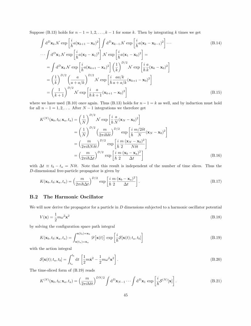
Suppose (B.13) holds for n− 1 = 1, 2, . . . , k − 1 for some k. Then by integrating k times we getˆ
dDxkN exp
[i
~a(xk+1 − xk)2
] ˆdDxk−1N exp
[i
~a(xk − xk−1)2
]· · · (B.14)
· · ·ˆ
dDx1N exp
[i
~a(x2 − x1)2
]N exp
[i
~a(x1 − x0)2
]=
=
ˆdDxkN exp
[i
~a(xk+1 − xk)2
](1
k
)D/2N exp
[i
~a
k(xk − x0)2
]=
(1
k
)D/2(a
a+ a/k
)D/2N exp
[i
~aa/k
a+ a/k(xk+1 − x0)2
]=
(1
k + 1
)D/2N exp
[i
~a
k + 1(xk+1 − x0)2
](B.15)
where we have used (B.10) once again. Thus (B.13) holds for n− 1 = k as well, and by induction must holdfor all n− 1 = 1, 2, . . .. After N − 1 integrations we therefore get
K(N)(xb, tb; xa, ta) =
(1
N
)D/2N exp
[i
~a
N(xN − x0)2
]=
(1
N
)D/2 ( m
2πi~δt
)D/2exp
[i
~m/2δt
N(xN − x0)2
]=( m
2πi~Nδt
)D/2exp
[i
~m
2
(xN − x0)2
Nδt
]=( m
2πi~∆t
)D/2exp
[i
~m
2
(xb − xa)2
∆t
](B.16)
with ∆t ≡ tb − ta = Nδt. Note that this result is independent of the number of time slices. Thus theD-dimensional free-particle propagator is given by
K(xb, tb; xa, ta) =( m
2πi~∆t
)D/2exp
[i
~m
2
(xb − xa)2
∆t
]. (B.17)
B.2 The Harmonic Oscillator
We will now derive the propagator for a particle in D dimensions subjected to a harmonic oscillator potential
V (x) =1
2mω2x2 (B.18)
by solving the configuration space path integral
K(xb, tb; xa, ta) =
ˆ x(tb)=xb
x(ta)=xa
D[x(t)
]exp
[i
~S[x(t); ta, tb]
](B.19)
with the action integral
S[x(t); ta, tb] =
ˆ tb
ta
dt
[1
2mx2 − 1
2mω2x2
]. (B.20)
The time-sliced form of (B.19) reads
K(N)(xb, tb; xa, ta) =( m
2πi~δt
)DN/2 ˆdDxN−1 · · ·
ˆdDx1 exp
[i
~S(N)[x]
]. (B.21)
45

Instead of using the expression (4.35) for the time-sliced action, we write it as
S(N)[x] =
N∑k=1
[1
2m
(∆xkδt
)2
− 1
2mω2
(x2k + x2
k−12
)]δt, (B.22)
which differs from (4.35) in that we have replaced V (x(tk)) with the average 12
[V (x(tk)) + V (x(tk−1))
], the
large N limit still being (B.20). We can then rewrite it as
S(N)[x] =
N∑k=1
m
2δt2
[(xk − xk−1)2 − ω2δt2
(x2k + x2
k−12
)]δt
=
N∑k=1
m
2δt
[(1− 1
2ω2δt2
)(x2k + x2
k−1)− 2xk · xk−1]
=
N∑k=1
[a1(x2
k + x2k−1)− 2b1xk · xk−1
](B.23)
with
a1 :=m
2δt
(1− 1
2ω2δt2
)and b1 :=
m
2δt. (B.24)
Also letting
N1 :=( m
2πi~δt
)D/2(B.25)
the time-sliced path integral (B.21) becomes
K(N)(xb, tb; xa, ta) = NN1
ˆdDxN−1 · · ·
ˆdDx1 exp
[i
~
N∑k=1
(a1(x2
k + x2k−1)− 2b1xk · xk−1
)]
=
ˆdDxN−1 · · ·
ˆdDx1
N∏k=1
N1 exp
[i
~
(a1(x2
k + x2k−1)− 2b1xk · xk−1
)]=
ˆdDxN−1 N1 exp
[i
~
(a1(x2
N + x2N−1)− 2b1xN · xN−1
)]· · ·
· · ·ˆ
dDx1 N1 exp
[i
~
(a1(x2
2 + x21)− 2b1x2 · x1
)]×
N1 exp
[i
~
(a1(x2
1 + x20)− 2b1x1 · x0
)]. (B.26)
The integral over x1 in (B.26) is a special case of the following integral in which we have replaced a1, b1 inthe last exponential with arbitrary nonzero constants a, b, and x2 with x′. We solve this case instead, forlater convenience:ˆ
dDx exp
[i
~
(a1(x′
2+ x2)− 2b1x
′ · x)]
exp
[i
~
(a(x2 + x2
0)− 2bx · x0
)]=
= exp
[i
~
(a1x′2 + ax2
0
)] ˆdDx exp
[i
~
((a1 + a)x2 − 2(b1x
′ + bx0) · x)]. (B.27)
Using (A.23), the integral on the right-hand side evaluates toˆ
dDx exp
[i
~
((a1 + a)x2 − 2(b1x
′ + bx0) · x)]
=
(iπ~a1 + a
)D/2exp
[− i~
(a1 + a)
(−2(b1x
′ + bx0)
2(a1 + a)
)2]
=
(iπ~a1 + a
)D/2exp
[− i~
(b1x′ + bx0)2
a1 + a
](B.28)
46
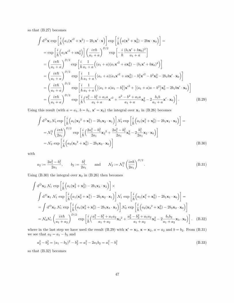
so that (B.27) becomes
ˆdDx exp
[i
~
(a1(x′
2+ x2)− 2b1x
′ · x)]
exp
[i
~
(a(x2 + x2
0)− 2bx · x0
)]=
= exp
[i
~
(a1x′2 + ax2
0
)]( iπ~a1 + a
)D/2exp
[− i~
(b1x′ + bx0)2
a1 + a
]=
(iπ~a1 + a
)D/2exp
[i
~1
a1 + a
((a1 + a)(a1x
′2 + ax20)− (b1x
′ + bx0)2)]
=
(iπ~a1 + a
)D/2exp
[i
~1
a1 + a
((a1 + a)(a1x
′2 + ax20)− b21x′
2 − b2x20 − 2b1bx
′ · x0
)]=
(iπ~a1 + a
)D/2exp
[i
~1
a1 + a
([(a1 + a)a1 − b21
]x′
2+[(a1 + a)a− b2
]x20 − 2b1bx
′ · x0
)]=
(iπ~a1 + a
)D/2exp
[i
~
(a21 − b21 + a1a
a1 + ax′
2+a2 − b2 + a1a
a1 + ax20 − 2
b1b
a1 + ax′ · x0
)]. (B.29)
Using this result (with a = a1, b = b1, x′ = x2) the integral over x1 in (B.26) becomes
ˆdDx1N1 exp
[i
~
(a1(x2
2 + x21)− 2b1x2 · x1
)]N1 exp
[i
~
(a1(x2
1 + x20)− 2b1x1 · x0
)]=
= N 21
(iπ~2a1
)D/2exp
[i
~
(2a21 − b212a1
x22 +
2a21 − b212a1
x20 − 2
b212a1
x2 · x0
)]= N2 exp
[i
~
(a2(x2
2 + x20)− 2b2x2 · x0
)](B.30)
with
a2 :=2a21 − b21
2a1, b2 :=
b212a1
and N2 := N 21
(iπ~2a1
)D/2. (B.31)
Using (B.30) the integral over x2 in (B.26) then becomes
ˆdDx2 N1 exp
[i
~
(a1(x2
3 + x22)− 2b1x3 · x2
)]×
ˆdDx1 N1 exp
[i
~
(a1(x2
2 + x21)− 2b1x2 · x1
)]N1 exp
[i
~
(a1(x2
1 + x20)− 2b1x1 · x0
)]=
=
ˆdDx2 N1 exp
[i
~
(a1(x2
3 + x22)− 2b1x3 · x2
)]N2 exp
[i
~
(a2(x2
2 + x20)− 2b2x2 · x0
)]= N2N1
(iπ~
a1 + a2
)D/2exp
[i
~
(a21 − b21 + a1a2a1 + a2
x32 +
a22 − b22 + a1a2a1 + a2
x20 − 2
b1b2a1 + a2
x3 · x0
)]. (B.32)
where in the last step we have used the result (B.29) with x′ = x3, x = x2, a = a2 and b = b2. From (B.31)we see that a2 = a1 − b2 and
a22 − b22 = (a1 − b2)2 − b22 = a21 − 2a1b2 = a21 − b21 (B.33)
so that (B.32) becomes
47
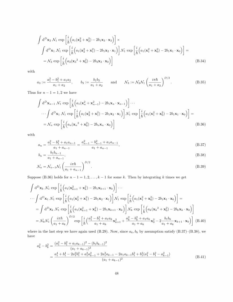
ˆdDx2 N1 exp
[i
~
(a1(x2
3 + x22)− 2b1x3 · x2
)]×
ˆdDx1 N1 exp
[i
~
(a1(x2
2 + x21)− 2b1x2 · x1
)]N1 exp
[i
~
(a1(x2
1 + x20)− 2b1x1 · x0
)]=
= N3 exp
[i
~
(a3(x3
2 + x20)− 2b3x3 · x0
)](B.34)
with
a3 :=a21 − b21 + a1a2
a1 + a2, b3 :=
b1b2a1 + a2
and N3 := N2N1
(iπ~
a1 + a2
)D/2. (B.35)
Thus for n− 1 = 1, 2 we have
ˆdDxn−1 N1 exp
[i
~
(a1(x2
n + x2n−1)− 2b1xn · xn−1
)]· · ·
· · ·ˆ
dDx1 N1 exp
[i
~
(a1(x2
2 + x21)− 2b1x2 · x1
)]N1 exp
[i
~
(a1(x2
1 + x20)− 2b1x1 · x0
)]=
= Nn exp
[i
~
(an(xn
2 + x20)− 2bnxn · x0
)](B.36)
with
an =a21 − b21 + a1an−1
a1 + an−1=a2n−1 − b2n−1 + a1an−1
a1 + an−1, (B.37)
bn =b1bn−1
a1 + an−1, (B.38)
Nn = Nn−1N1
(iπ~
a1 + an−1
)D/2. (B.39)
Suppose (B.36) holds for n− 1 = 1, 2, . . . , k − 1 for some k. Then by integrating k times we get
ˆdDxk N1 exp
[i
~
(a1(x2
k+1 + x2k)− 2b1xk+1 · xk
)]· · ·
· · ·ˆ
dDx1 N1 exp
[i
~
(a1(x2
2 + x21)− 2b1x2 · x1
)]N1 exp
[i
~
(a1(x2
1 + x20)− 2b1x1 · x0
)]=
=
ˆdDxk N1 exp
[i
~
(a1(x2
k+1 + x2k)− 2b1xk+1 · xk
)]Nk exp
[i
~
(ak(xk
2 + x20)− 2bkxk · x0
)]= NkN1
(iπ~
a1 + ak
)D/2exp
[i
~
(a21 − b21 + a1aka1 + ak
x2k+1 +
a2k − b2k + a1aka1 + ak
x20 − 2
b1bka1 + ak
xk+1 · x0
)](B.40)
where in the last step we have again used (B.29). Now, since ak, bk by assumption satisfy (B.37)–(B.38), wehave
a2k − b2k =(a21 − b21 + a1ak−1)2 − (b1bk−1)2
(a1 + ak−1)2
=a41 + b41 − 2a21b
21 + a21a
2k−1 + 2a31ak−1 − 2a1ak−1b
21 + b21(a21 − b21 − a2k−1)
(a1 + ak−1)2(B.41)
48
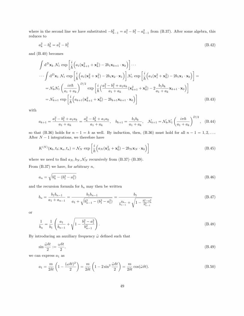
where in the second line we have substituted −b2k−1 = a21 − b21 − a2k−1 from (B.37). After some algebra, thisreduces to
a2k − b2k = a21 − b21 (B.42)
and (B.40) becomes
ˆdDxk N1 exp
[i
~
(a1(x2
k+1 + x2k)− 2b1xk+1 · xk
)]· · ·
· · ·ˆ
dDx1 N1 exp
[i
~
(a1(x2
2 + x21)− 2b1x2 · x1
)]N1 exp
[i
~
(a1(x2
1 + x20)− 2b1x1 · x0
)]=
= NkN1
(iπ~
a1 + ak
)D/2exp
[i
~
(a21 − b21 + a1aka1 + ak
(x2k+1 + x2
0)− 2b1bk
a1 + akxk+1 · x0
)]= Nk+1 exp
[i
~
(ak+1(x2
k+1 + x20)− 2bk+1xk+1 · x0
)](B.43)
with
ak+1 =a21 − b21 + a1ak
a1 + ak=a2k − b2k + a1ak
a1 + ak, bk+1 =
b1bka1 + ak
, Nk+1 = NkN1
(iπ~
a1 + ak
)D/2, (B.44)
so that (B.36) holds for n − 1 = k as well. By induction, then, (B.36) must hold for all n − 1 = 1, 2, . . ..After N − 1 integrations, we therefore have
K(N)(xb, tb; xa, ta) = NN exp
[i
~
(aN (x2
N + x20)− 2bNxN · x0
)](B.45)
where we need to find aN , bN ,NN recursively from (B.37)–(B.39).
From (B.37) we have, for arbitrary n,
an =√b2n − (b21 − a21) (B.46)
and the recursion formula for bn may then be written
bn =b1bn−1
a1 + an−1=
b1bn−1
a1 +√b2n−1 − (b21 − a21)
=b1
a1bn−1
+
√1− b21−a21
b2n−1
(B.47)
or
1
bn=
1
b1
(a1bn−1
+
√1− b21 − a21
b2n−1
). (B.48)
By introducing an auxiliary frequency ω defined such that
sinωδt
2:=
ωδt
2, (B.49)
we can express a1 as
a1 =m
2δt
(1− (ωδt)2
2
)=
m
2δt
(1− 2 sin2 ωδt
2
)=
m
2δtcos(ωδt). (B.50)
49

The relation (B.48) then becomes
1
bn=
1m2δt
m2δt cos(ωδt)
bn−1+
√1−
m2
4δt2 −m2
4δt2 cos2(ωδt)
b2n−1
=
cos(ωδt)
bn−1+
2δt
m
√1− m2
4δt2sin2(ωδt)
b2n−1. (B.51)
For notational convenience, we now introduce reduced quantities
βn :=bnb1
=2δt
mbn. (B.52)
Then the recursion formula for βn reads
1
βn=
cos(ωδt)
βn−1+
√1− sin2(ωδt)
β2n−1
(B.53)
with β1 = 1. For n = 2, 3 we get
1
β2= cos(ωδt) +
√1− sin2(ωδt) =
sin(2ωδt)
sin(ωδt)(B.54)
and
1
β3= cos(ωδt)
sin(2ωδt)
sin(ωδt)+
√1− sin2(ωδt)
sin2(2ωδt)
sin2(ωδt)=
sin(3ωδt)
sin(ωδt), (B.55)
so in general we expect that
1
βn=
sin(nωδt)
sin(ωδt). (B.56)
Suppose (B.56) holds for all n = 1, 2, . . . , k for some k. Then
1
βk+1= cos(ωδt)
sin(kωδt)
sin(ωδt)+
√1− sin2(ωδt)
sin2(kωδt)
sin2(ωδt)=
sin((k + 1)ωδt)
sin(ωδt)(B.57)
so that (B.56) holds for k + 1 as well. By induction it must hold for all n = 1, 2, . . . and hence solves therecursion relation (B.53). Thus we have
bn =m
2δtβn =
m
2δt
sin(ωδt)
sin(nωδt). (B.58)
From (B.46) and (B.50) we then get
an =√b2n − (b21 − a21) =
√( m2δt
)2 sin2(ωδt)
sin2(nωδt)−[( m
2δt
)2−( m
2δt
)2cos2(ωδt)
]
=m
2δt
√sin2(ωδt)
sin2(nωδt)− sin2(ωδt) =
m
2δtsin(ωδt)
cos(nωδt)
sin(nωδt). (B.59)
50

We have now determined the an and the bn. Finally, we need to determine the normalisation constant (B.39).For n = 2, 3 we get
N2 = N1N1
(iπ~
a1 + a1
)D/2= N 2
1
(iπ~
2 m2δt cos(ωδt)
)D/2= N1
(sin(ωδt)
sin(2ωδt)
)D/2(B.60)
and
N3 = N2N1
(iπ~
a1 + a2
)D/2= N 2
1
(sin(ωδt)
sin(2ωδt)
)D/2 iπ~m2δt
(cos(ωδt) + sin(ωδt) cos(2ωδt)
sin(2ωδt)
)D/2
= N1
(sin(ωδt)
sin(3ωδt)
)D/2(B.61)
so we expect the general result
Nn = N1
(sin(ωδt)
sin(nωδt)
)D/2. (B.62)
Suppose (B.62) holds for all n = 1, 2, . . . , k for some k. Then
Nk+1 = NkN1
(iπ~
a1 + ak
)D/2= N 2
1
(sin(ωδt)
sin(kωδt)
)D/2 iπ~m2δt
(cos(ωδt) + sin(ωδt) cos(kωδt)
sin(kωδt)
)D/2
= N1
(sin(ωδt)
sin((k + 1)ωδt)
)D/2, (B.63)
so that (B.62) holds for k + 1 as well. By induction it must hold for all n = 1, 2, . . . and hence solves therecursion relation (B.39). Having obtained the constants (B.59), (B.58) and (B.62), we now plug them into(B.45) and get
K(N)(xb, tb; xa, ta) =
= NN exp
[i
~
(aN (x2
N + x20)− 2bNxN · x0
)]= N1
(sin(ωδt)
sin(Nωδt)
)D/2exp
[i
~
( m2δt
sin(ωδt)cos(Nωδt)
sin(Nωδt)(x2N + x2
0)− 2m
2δt
sin(ωδt)
sin(Nωδt)xN · x0
)]=( m
2πi~δt
)D/2( sin(ωδt)
sin(Nωδt)
)D/2exp
[i
~m
2δt
sin(ωδt)
sin(Nωδt)
((x2N + x2
0) cos(Nωδt)− 2xN · x0
)]=
(m
2πi~ω
sin(Nωδt)
sin(ωδt)
ωδt
)D/2exp
[i
~mω
2 sin(Nωδt)
sin(ωδt)
ωδt
((x2N + x2
0) cos(Nωδt)− 2xN · x0
)]=
(m
2πi~ω
sin(ω∆t)
sin(ωδt)
ωδt
)D/2exp
[i
~mω
2 sin(ω∆t)
sin(ωδt)
ωδt
((x2b + x2
a) cos(ω∆t)− 2xb · xa)]
(B.64)
with ∆t ≡ tb − ta = Nδt. In taking the limit N → ∞, δt → 0, we have sin(ωδt)ωδt → 1 and the auxiliary
frequency ω defined by (B.49) simply becomes the oscillator frequency ω. We then finally obtain the followingexpression for the propagator of the D-dimensional harmonic oscillator:
K(xb, tb; xa, ta) =
(mω
2πi~ sin(ω∆t)
)D/2exp
[i
~mω
2 sin(ω∆t)
((x2b + x2
a) cos(ω∆t)− 2xb · xa)]. (B.65)
51

C Square-root Coordinates for the 3-D H-atom
For the solution of the path integral for the three-dimensional Hydrogen atom, we introduced a mappingfrom a four-dimensional {uµ} space to the three-dimensional {xi} space by
xi = z†σiz (C.1)
with
z =
[z1z2
]:=
[u1 + iu2
u3 + iu4
](C.2)
and the Pauli spin matrices
σ1 =
[0 11 0
]σ2 =
[0 −ii 0
]σ3 =
[1 00 −1
]. (C.3)
Explicitly, the transformation (C.1) readsx1x2x3
=
z†σ1zz†σ2zz†σ3z
=
z∗1z2 + z∗2z1−iz∗1z2 + iz∗2z1z∗1z1 − z∗2z2
=
2 Re(z∗1z2)2 Im(z∗1z2)|z1|2 − |z2|2
=
2u1u3 + 2u2u4
2u1u4 − 2u2u3
(u1)2 + (u2)2 − (u3)2 − (u4)2
(C.4)
and the relations between the differentials aredx1
dx2
dx3
=
2u3 2u4 2u1 2u2
2u4 −2u3 −2u2 2u1
2u1 2u2 −2u3 −2u4
du1
du2
du3
du4
. (C.5)
The transformation (C.1) has been chosen so that r = ~u2. Indeed, we have
r2 =∑i
(xi)2 = (z∗1z2 + z∗2z1)2 + (−iz∗1z2 + iz∗2z1)2 + (z∗1z1 − z∗2z2)2 = (|z1|2 + |z2|2)2 (C.6)
so that
r = |z1|2 + |z2|2 = (u1)2 + (u2)2 + (u3)2 + (u4)2 ≡ ~u2. (C.7)
The mapping (C.4) is obviously not invertible, so the inverse relationship will be multivalued. To find aninverse relationship, we first express the xi in terms of spherical coordinates x1 = r sin θ cosφ
x2 = r sin θ sinφx3 = r cos θ
. (C.8)
Next, by writing
z1 = |z1| exp [iθ1] , z2 = |z2| exp [iθ2] (C.9)
we have, from (C.4) and (C.7),{|z1|2 + |z2|2 = r
|z1|2 − |z2|2 = r cos θor
{|z1|2 = 1
2r(1 + cos θ) = r cos2(θ/2)
|z2|2 = 12r(1− cos θ) = r sin2(θ/2)
(C.10)
52

giving{z1 =
√r cos(θ/2) exp [iθ1]
z2 =√r sin(θ/2) exp [iθ2]
. (C.11)
To find the phase angles, we calculate
z∗1z2 = r cos(θ/2) sin(θ/2) exp [i(θ2 − θ1)] =1
2r sin θ exp [i(θ2 − θ1)] (C.12)
and use, from (C.4),
r sin θ cosφ = x1 = 2 Re(z∗1z2) = r sin θ cos(θ2 − θ1) (C.13)
and
r sin θ sinφ = x2 = 2 Im(z∗1z2) = r sin θ sin(θ2 − θ1), (C.14)
to find that
θ2 − θ1 = φ+ 2πn. (C.15)
Letting
θ1 = −φ+ γ
2, with γ ∈ R, (C.16)
then gives us
θ2 = −φ+ γ
2+ φ+ 2πn =
φ− γ2
+ 2πn. (C.17)
Thus {z1 =
√r cos(θ/2) exp [−i(φ+ γ)/2]
z2 =√r sin(θ/2) exp [i(φ− γ)/2]
(C.18)
or
u1 =√r cos
(θ2
)cos(φ+γ2
)u2 = −
√r cos
(θ2
)sin(φ+γ2
)u3 =
√r sin
(θ2
)cos(φ−γ2
)u4 =
√r sin
(θ2
)sin(φ−γ2
) . (C.19)
For fixed (r, θ, φ), this describes a curve in {uµ} space parametrized by γ. Each point on this curve maps tothe same point (r, θ, φ) in {xi} space. Note that the curve is closed, since uµ(γ + 4π) = uµ(γ). Thus we canrestrict γ to the interval [0, 4π).
We can then interpret γ as an additional angle that compliments r, θ, φ as coordinates for the four-dimensional{uµ} space. Accordingly, we introduce a fourth coordinate x4 and extend the mapping from uµ to xi by thedifferential relation
dx4 = 2u2 du1 − 2u1 du2 + 2u4 du3 − 2u3 du4 (C.20)
so thatdx1
dx2
dx3
dx4
=
2u3 2u4 2u1 2u2
2u4 −2u3 −2u2 2u1
2u1 2u2 −2u3 −2u4
2u2 −2u1 2u4 −2u3
du1
du2
du3
du4
(C.21)
53

or
[d~x] = A(~u)[d~u] (C.22)
with the Jacobian matrix
A(~u) =
2u3 2u4 2u1 2u2
2u4 −2u3 −2u2 2u1
2u1 2u2 −2u3 −2u4
2u2 −2u1 2u4 −2u3
. (C.23)
The relation (C.20) has been chosen such that the metric in uµ coordinates,
gµν =∂xα
∂uµ∂xβ
∂uνδαβ (summation convention implied), (C.24)
takes the simple form
g(~u) = ATA = 4
u3 u4 u1 u2
u4 −u3 u2 −u1u1 −u2 −u3 u4
u2 u1 −u4 −u3
u3 u4 u1 u2
u4 −u3 −u2 u1
u1 u2 −u3 −u4u2 −u1 u4 −u3
= 4
~u2 0 0 00 ~u2 0 00 0 ~u2 00 0 0 ~u2
= 4rI (C.25)
so that the determinant of A is
|det A| =√
det g =√
(4r)4 = 16r2. (C.26)
Note that the relation (C.20) is not integrable since the mixed partial derivatives don’t commute, e.g.:
∂2x4
∂u2∂u1= − ∂2x4
∂u1∂u2. (C.27)
Nevertheless, the relation between {xµ} and {uµ} becomes bijective once it has been specified at an initialpoint uµ(~xa) = uµa .
Using the relations in (C.19) we can express the differentials duµ in terms of (dr, dθ,dφ, dγ) and substitutethese into (C.20) to find
dx4 = r cos θ dφ+ r dγ. (C.28)
54

References
[1] Wikipedia contributors. Path integral formulation [Internet]. Wikipedia, The Free Encyclopedia; 2016May 7 [cited 2015 May 23]. Available from: https://en.wikipedia.org/wiki/Path_integral_
formulation
[2] Duru, I. H. and Kleinert, H., Solution of the path integral for the H-atom, Physics Letters vol. 84B,number 2, 185–188 (1979)
[3] Duru, I. H. and Kleinert, H., Quantum Mechanics of H-atom from Path Integrals, Fortschritte derPhysik 30, 401–435 (1982)
[4] Kleinert, H., 2004, Path Integrals in Quantum Mechanics, Statistics, Polymer Physics, and FinancialMarkets, 3rd ed., World Scientific, 1468 p.
[5] Glimm, J. and Jaffe, A., 1981, Quantum Physics, A Functional Integral Point of View, 2nd ed., Springer,535 p.
[6] Wikipedia contributors. Jacobi–Anger expansion [Internet]. Wikipedia, The Free Encyclopedia; 2015May 8 [cited 2015 May 23]. Available from: https://en.wikipedia.org/wiki/Jacobi-Anger_
expansion
[7] Kleinert, H., Path Integral of Relativistic Coulomb System, Physics Letters vol. A 212, number 15,15–21 (1996)
55