Guidelines for the Use of Mobile LIDAR in

Transportation Applications

NCHRP REPORT 748

NATIONALCOOPERATIVEHIGHWAYRESEARCHPROGRAM

TRANSPORTATION RESEARCH BOARD 2013 EXECUTIVE COMMITTEE*

OFFICERS

Chair: Deborah H. Butler, Executive Vice President, Planning, and CIO, Norfolk Southern Corporation, Norfolk, VA ViCe Chair: Kirk T. Steudle, Director, Michigan DOT, LansingexeCutiVe DireCtor: Robert E. Skinner, Jr., Transportation Research Board

MEMBERS

Victoria A. Arroyo, Executive Director, Georgetown Climate Center, and Visiting Professor, Georgetown University Law Center, Washington, DC

Scott E. Bennett, Director, Arkansas State Highway and Transportation Department, Little RockWilliam A. V. Clark, Professor of Geography (emeritus) and Professor of Statistics (emeritus), Department of Geography, University of

California, Los AngelesJames M. Crites, Executive Vice President of Operations, Dallas–Fort Worth International Airport, TXMalcolm Dougherty, Director, California Department of Transportation, SacramentoJohn S. Halikowski, Director, Arizona DOT, PhoenixMichael W. Hancock, Secretary, Kentucky Transportation Cabinet, FrankfortSusan Hanson, Distinguished University Professor Emerita, School of Geography, Clark University, Worcester, MA Steve Heminger, Executive Director, Metropolitan Transportation Commission, Oakland, CAChris T. Hendrickson, Duquesne Light Professor of Engineering, Carnegie Mellon University, Pittsburgh, PAJeffrey D. Holt, Managing Director, Bank of Montreal Capital Markets, and Chairman, Utah Transportation Commission, Huntsville, UTGary P. LaGrange, President and CEO, Port of New Orleans, LAMichael P. Lewis, Director, Rhode Island DOT, ProvidenceJoan McDonald, Commissioner, New York State DOT, AlbanyDonald A. Osterberg, Senior Vice President, Safety and Security, Schneider National, Inc., Green Bay, WISteve Palmer, Vice President of Transportation, Lowe’s Companies, Inc., Mooresville, NCSandra Rosenbloom, Director, Innovation in Infrastructure, The Urban Institute, Washington, DCHenry G. (Gerry) Schwartz, Jr., Chairman (retired), Jacobs/Sverdrup Civil, Inc., St. Louis, MOKumares C. Sinha, Olson Distinguished Professor of Civil Engineering, Purdue University, West Lafayette, INDaniel Sperling, Professor of Civil Engineering and Environmental Science and Policy; Director, Institute of Transportation Studies;

University of California, DavisGary C. Thomas, President and Executive Director, Dallas Area Rapid Transit, Dallas, TXPhillip A. Washington, General Manager, Regional Transportation District, Denver, CO

EX OFFICIO MEMBERS

Rebecca M. Brewster, President and COO, American Transportation Research Institute, Marietta, GA Anne S. Ferro, Administrator, Federal Motor Carrier Safety Administration, U.S. DOT LeRoy Gishi, Chief, Division of Transportation, Bureau of Indian Affairs, U.S. Department of the Interior, Washington, DCJohn T. Gray II, Senior Vice President, Policy and Economics, Association of American Railroads, Washington, DCMichael P. Huerta, Administrator, Federal Aviation Administration, U.S. DOT David T. Matsuda, Administrator, Maritime Administration, U.S. DOT Michael P. Melaniphy, President and CEO, American Public Transportation Association, Washington, DCVictor M. Mendez, Administrator, Federal Highway Administration, U.S. DOT Robert J. Papp (Adm., U.S. Coast Guard), Commandant, U.S. Coast Guard, U.S. Department of Homeland SecurityLucy Phillips Priddy, Research Civil Engineer, U.S. Army Corps of Engineers, Vicksburg, MS, and Chair, TRB Young Members Council,

Washington, DCCynthia L. Quarterman, Administrator, Pipeline and Hazardous Materials Safety Administration, U.S. DOTPeter M. Rogoff, Administrator, Federal Transit Administration, U.S. DOTDavid L. Strickland, Administrator, National Highway Traffic Safety Administration, U.S. DOTJoseph C. Szabo, Administrator, Federal Railroad Administration, U.S. DOTPolly Trottenberg, Under Secretary for Policy, U.S. DOT Robert L. Van Antwerp (Lt. General, U.S. Army), Chief of Engineers and Commanding General, U.S. Army Corps of Engineers,

Washington, DCBarry R. Wallerstein, Executive Officer, South Coast Air Quality Management District, Diamond Bar, CA Gregory D. Winfree, Acting Administrator, Research and Innovative Technology Administration,

U.S. DOTFrederick G. (Bud) Wright, Executive Director, American Association of State Highway and Transportation Officials, Washington, DC

*Membership as of April 2013.

N A T I O N A L C O O P E R A T I V E H I G H W A Y R E S E A R C H P R O G R A M

NCHRP REPORT 748

Guidelines for the Use of Mobile LIDAR in

Transportation Applications

Michael J. OlsenOregOn State UniverSity

Corvallis, OR

Gene V. RoeMPn COMPOnentS

Hampton, NH

Craig GlennieUniverSity Of HOUStOn

Houston, TX

Fred PersiPerSi COnSUlting

Aliquippa, PA

Marcus ReedyDaviD evanS anD aSSOCiateS

Portland, OR

David Hurwitz, Keith Williams, and Halston TussOregOn State UniverSity

Corvallis, OR

Anthony SquellatiDaviD evanS anD aSSOCiateS

Roseville, CA

Michael KnodlerinnOvative Data inC.

Belchertown, MA

Subscriber Categories

Highways • Data and Information • Design • Planning and Forecasting

TRANSPORTAT ION RESEARCH BOARDWASHINGTON, D.C.

2013www.TRB.org

Research sponsored by the American Association of State Highway and Transportation Officials in cooperation with the Federal Highway Administration

NATIONAL COOPERATIVE HIGHWAY RESEARCH PROGRAM

Systematic, well-designed research provides the most effective

approach to the solution of many problems facing highway

administrators and engineers. Often, highway problems are of local

interest and can best be studied by highway departments individually

or in cooperation with their state universities and others. However, the

accelerating growth of highway transportation develops increasingly

complex problems of wide interest to highway authorities. These

problems are best studied through a coordinated program of

cooperative research.

In recognition of these needs, the highway administrators of the

American Association of State Highway and Transportation Officials

initiated in 1962 an objective national highway research program

employing modern scientific techniques. This program is supported on

a continuing basis by funds from participating member states of the

Association and it receives the full cooperation and support of the

Federal Highway Administration, United States Department of

Transportation.

The Transportation Research Board of the National Academies was

requested by the Association to administer the research program

because of the Board’s recognized objectivity and understanding of

modern research practices. The Board is uniquely suited for this

purpose as it maintains an extensive committee structure from which

authorities on any highway transportation subject may be drawn; it

possesses avenues of communications and cooperation with federal,

state and local governmental agencies, universities, and industry; its

relationship to the National Research Council is an insurance of

objectivity; it maintains a full-time research correlation staff of specialists

in highway transportation matters to bring the findings of research

directly to those who are in a position to use them.

The program is developed on the basis of research needs identified

by chief administrators of the highway and transportation departments

and by committees of AASHTO. Each year, specific areas of research

needs to be included in the program are proposed to the National

Research Council and the Board by the American Association of State

Highway and Transportation Officials. Research projects to fulfill these

needs are defined by the Board, and qualified research agencies are

selected from those that have submitted proposals. Administration and

surveillance of research contracts are the responsibilities of the National

Research Council and the Transportation Research Board.

The needs for highway research are many, and the National

Cooperative Highway Research Program can make significant

contributions to the solution of highway transportation problems of

mutual concern to many responsible groups. The program, however, is

intended to complement rather than to substitute for or duplicate other

highway research programs.

Published reports of the

NATIONAL COOPERATIVE HIGHWAY RESEARCH PROGRAM

are available from:

Transportation Research BoardBusiness Office500 Fifth Street, NWWashington, DC 20001

and can be ordered through the Internet at:

http://www.national-academies.org/trb/bookstore

Printed in the United States of America

NCHRP REPORT 748

Project 15-44 ISSN 0077-5614 ISBN 978-0-309-25914-9 Library of Congress Control Number 2013939444

© 2013 National Academy of Sciences. All rights reserved.

COPYRIGHT INFORMATION

Authors herein are responsible for the authenticity of their materials and for obtaining written permissions from publishers or persons who own the copyright to any previously published or copyrighted material used herein.

Cooperative Research Programs (CRP) grants permission to reproduce material in this publication for classroom and not-for-profit purposes. Permission is given with the understanding that none of the material will be used to imply TRB, AASHTO, FAA, FHWA, FMCSA, FTA, or Transit Development Corporation endorsement of a particular product, method, or practice. It is expected that those reproducing the material in this document for educational and not-for-profit uses will give appropriate acknowledgment of the source of any reprinted or reproduced material. For other uses of the material, request permission from CRP.

NOTICE

The project that is the subject of this report was a part of the National Cooperative Highway Research Program, conducted by the Transportation Research Board with the approval of the Governing Board of the National Research Council.

The members of the technical panel selected to monitor this project and to review this report were chosen for their special competencies and with regard for appropriate balance. The report was reviewed by the technical panel and accepted for publication according to procedures established and overseen by the Transportation Research Board and approved by the Governing Board of the National Research Council.

The opinions and conclusions expressed or implied in this report are those of the researchers who performed the research and are not necessarily those of the Transportation Research Board, the National Research Council, or the program sponsors.

The Transportation Research Board of the National Academies, the National Research Council, and the sponsors of the National Cooperative Highway Research Program do not endorse products or manufacturers. Trade or manufacturers’ names appear herein solely because they are considered essential to the object of the report.

The National Academy of Sciences is a private, nonprofit, self-perpetuating society of distinguished scholars engaged in scientific

and engineering research, dedicated to the furtherance of science and technology and to their use for the general welfare. On the

authority of the charter granted to it by the Congress in 1863, the Academy has a mandate that requires it to advise the federal

government on scientific and technical matters. Dr. Ralph J. Cicerone is president of the National Academy of Sciences.

The National Academy of Engineering was established in 1964, under the charter of the National Academy of Sciences, as a parallel

organization of outstanding engineers. It is autonomous in its administration and in the selection of its members, sharing with the

National Academy of Sciences the responsibility for advising the federal government. The National Academy of Engineering also

sponsors engineering programs aimed at meeting national needs, encourages education and research, and recognizes the superior

achievements of engineers. Dr. Charles M. Vest is president of the National Academy of Engineering.

The Institute of Medicine was established in 1970 by the National Academy of Sciences to secure the services of eminent members

of appropriate professions in the examination of policy matters pertaining to the health of the public. The Institute acts under the

responsibility given to the National Academy of Sciences by its congressional charter to be an adviser to the federal government

and, on its own initiative, to identify issues of medical care, research, and education. Dr. Harvey V. Fineberg is president of the

Institute of Medicine.

The National Research Council was organized by the National Academy of Sciences in 1916 to associate the broad community of

science and technology with the Academy’s purposes of furthering knowledge and advising the federal government. Functioning in

accordance with general policies determined by the Academy, the Council has become the principal operating agency of both the

National Academy of Sciences and the National Academy of Engineering in providing services to the government, the public, and

the scientific and engineering communities. The Council is administered jointly by both Academies and the Institute of Medicine.

Dr. Ralph J. Cicerone and Dr. Charles M. Vest are chair and vice chair, respectively, of the National Research Council.

The Transportation Research Board is one of six major divisions of the National Research Council. The mission of the Transporta-

tion Research Board is to provide leadership in transportation innovation and progress through research and information exchange,

conducted within a setting that is objective, interdisciplinary, and multimodal. The Board’s varied activities annually engage about

7,000 engineers, scientists, and other transportation researchers and practitioners from the public and private sectors and academia,

all of whom contribute their expertise in the public interest. The program is supported by state transportation departments, federal

agencies including the component administrations of the U.S. Department of Transportation, and other organizations and individu-

als interested in the development of transportation. www.TRB.org

www.national-academies.org

C O O P E R A T I V E R E S E A R C H P R O G R A M S

AUTHOR ACKNOWLEDGMENTS

The research reported herein was performed under NCHRP Project 15-44 by the School of Civil and Construction Engineering at Oregon State University (OSU), the National Center for Airborne Laser Mapping (NCALM) at the University of Houston (UofH), MPN Components, David Evans & Associates, Persi Consulting, and Innovative Data, Inc. Dr. Michael J. Olsen, Assistant Professor of Civil Engineering Geomatics at OSU, was the Project Director and Principal Investigator. The other authors of this report are Dr. Craig Glennie, UofH and Co-Principal Investigator; Dr. Gene V. Roe, of MPN; Marcus Reedy, Vice President, Director of Geomatics at David Evans and Associates; and Dr. Fred Persi, President of Persi Consulting. Keith Williams, Research Assistant at OSU; Dr. David Hurwitz, Assistant Professor of Civil Engineering Transportation at OSU; Halston Tuss, Research Assistant at OSU; Anthony Squellati, of David Evans and Associates; and Dr. Michael Knodler, Innovative Data Inc. were authors of material included in Appendixes A, B, and G and provided other contributions throughout the report. Special thanks also go to the Government of Alberta Ministry of Transportation, Central Federal Lands Highway Division, Mainroads Western Australia, and Tran systems for their willingness to help with this research task and to the mobile LIDAR service providers who provided their expertise.

CRP STAFF FOR NCHRP REPORT 748

Christopher W. Jenks, Director, Cooperative Research ProgramsCrawford F. Jencks, Deputy Director, Cooperative Research ProgramsEdward T. Harrigan, Senior Program OfficerAnthony Avery, Senior Program AssistantEileen P. Delaney, Director of PublicationsSharon Lamberton, Assistant Editor

NCHRP PROJECT 15-44 PANELDesign—General Design

Thomas Taylor, Oakland, CA (Chair)Eric Jackson, Washington State DOT, Tumwater, WAMichael F. Balbierer, Delaware DOT, Dover, DELewis N. Graham, GeoCue Corporation, Madison, ALChristopher C. Harris, Tennessee DOT, Nashville, TNAlexa B. Mitchell, Missouri DOT, Jefferson City, MORobert G. Rausch, TransCore ITS, LLC, Norcross, GALincoln Cobb, FHWA LiaisonThomas Palmerlee, TRB Liaison

F O R E W O R D

By Edward T. HarriganStaff OfficerTransportation Research Board

This report presents guidelines for the application of mobile 3D light detection and rang-ing (LIDAR) technology to the operations of state departments of transportation. The guide will be of immediate interest to management and technical staff of the departments respon-sible for procurement of this technology and its use in the planning, design, construction, and maintenance of transportation facilities.

NCHRP Project 15-44, “Guidelines for the Use of Mobile LIDAR in Transportation Applications,” was conducted by Oregon State University, Corvallis, Oregon, with the participation of (1) MPN Components, Hampton, New Hampshire, (2) the University of Houston, Houston, Texas, (3) Persi Consulting, Aliquippa, Pennsylvania, (4) David Evans and Associates, Portland, Oregon, and (5) Innovative Data, Inc., Belchertown, Massachusetts.

The objective of the project was to develop guidelines for the use of mobile LIDAR tech-nology in transportation applications. The guidelines (1) are based on an analysis of cur-rent and emerging applications in areas such as project planning, project development, construction, operations, maintenance, safety, research, and asset management; (2) address data collection methods, formatting and management, storage requirements, quality assur-ance, and the translation and formatting of derived products; and (3) are based on and organized around performance criteria such as data precision, local (relative) accuracy, network (absolute) accuracy, and point density.

Mobile LIDAR uses laser scanning equipment mounted on vehicles in combination with global positioning systems (GPS) and inertial measurement units (IMU) to rapidly and safely capture large datasets necessary to create highly accurate, high resolution digital rep-resentations of roadways and their surroundings. (Aerial LIDAR, which performs the same function from aircraft, was not within the scope of this project.) These virtual survey data-sets can then be used in the planning, design, construction, and maintenance of highways and structures as well as for numerous other functions as varied as emergency response and asset management.

The development of the guidelines comprised several major tasks. The research team first conducted an extensive review of the worldwide literature on the use of mobile LIDAR. Emphasis was placed on exploring current mobile LIDAR trends, including systems com-ponents and software, and identifying current and emerging applications of mobile LIDAR for transportation agencies. Of particular interest was an analysis of quality control proce-dures used to verify the accuracy of the data collected with mobile LIDAR. The literature review was supported by a questionnaire administered to the state departments of trans-portation, other transportation agencies, and industry. Finally, projects piloting mobile

LIDAR technology on network and local levels were identified and evaluated in depth. This information provided a solid foundation for developing the actual guidelines.

The guidelines are organized into two parts. Part 1: Management and Decision Mak-ing provides guidance on the use and integration of mobile LIDAR data for a wide range of transportation applications without requiring in-depth knowledge of the technology; Part 2: Technical Considerations provides the details needed to completely specify the proj-ect requirements and appropriate deliverables. The following appendixes included with the guidelines document the entire research effort as well as other resources for implementing the guidelines:

• Appendix A: Literature Review• Appendix B: Questionnaire Report• Appendix C: Statement of Work (Outline)• Appendix D: Sample Calibration Report• Appendix E: Current Storage Formats• Appendix F: Additional Considerations• Appendix G: Glossary

C O N T E N T S

1 Summary

3 Chapter 1 Objectives 3 1.1 Motivation and Requirements for National Transportation

Agency Guidelines

5 Chapter 2 Overview 5 2.1 Development 5 2.1.1 Literature Review 5 2.1.2 Questionnaires 6 2.2 Organization of NCHRP Report 748

P A R T 1 Management and Decision Making

9 Chapter 3 Applications 9 3.1 Applicability 9 3.2 Data Collection Procurement Categories 10 3.3 Suggested Accuracy Levels for Transportation Applications

12 Chapter 4 Workflow and Data Management 12 4.1 Workflow Stages 12 4.1.1 Data Acquisition 12 4.1.2 Georeferencing 12 4.1.3 Post-processing 13 4.1.4 Computation and Analysis 13 4.1.5 Packaging and Delivery 13 4.2 Models vs. Point Clouds 14 4.3 Coverage 14 4.4 Sequential and Traceable Processes 14 4.5 Considerations for Information Technology 14 4.5.1 File Management 15 4.5.2 Information Transfer Latency 15 4.5.3 Accessibility and Security 15 4.5.4 Integrity 15 4.5.5 Sunset Plan 15 4.5.6 Software 16 4.5.7 Hardware

17 Chapter 5 Organizational Data Mining 17 5.1 Single Repository 17 5.2 Historical 17 5.3 Faster Decisions

17 5.4 Costs 17 5.5 Redundancy

19 Chapter 6 Procurement Considerations 19 6.1 Decision Process 21 6.2 Generic Cost Considerations 22 6.3 System Ownership 23 6.3.1 Owner/Operator 23 6.3.2 Professional Consultant Services

24 Chapter 7 Implementation Plan for Transportation Agencies 24 7.1 Intent 24 7.2 Background 24 7.2.1 The 3D Technology Revolution 24 7.2.2 Mobile LIDAR 24 7.2.3 Organizational Change 25 7.3 Strategic Plan 25 7.4 Innovation Group 25 7.5 Implementing the Guidelines 26 7.6 Documenting Results 27 7.7 Workflow Integration 27 7.8 Future Opportunities

28 Chapter 8 Currently Available Guidelines 28 8.1 Geospatial Data Accuracy 29 8.2 ASPRS Guidelines 29 8.3 Transportation Agency LIDAR Standards 30 8.4 FAA Advisory Circular

P A R T 2 Technical Considerations

33 Chapter 9 Background 33 9.1 Typical MLS Components 33 9.1.1 Laser Scanners 33 9.1.2 GNSS Receivers 34 9.1.3 IMUs 34 9.1.4 Distance Measurement Indicators (DMIs) 34 9.1.5 Digital Cameras 35 9.1.6 Rigid Platform 35 9.1.7 Other Ancillary Devices 35 9.2 Comparison to ALS 36 9.3 Calculation of Ground Coordinates from MLS Data

38 Chapter 10 Accuracy of Components 38 10.1 Typical Size of Error Parameters 38 10.2 IMU Attitude Errors 38 10.3 Boresight Errors 38 10.4 Laser Scanner Errors 39 10.4.1 Lever Arm Offset Errors 40 10.5 Positioning Errors 40 10.6 Overall System Accuracy

41 Chapter 11 Calibration and Correction 41 11.1 System Calibration 41 11.2 Geometric Correction

42 Chapter 12 Accuracy and Point Density Specification 42 12.1 Point Cloud Accuracy Levels 42 12.1.1 Accuracy Specification for MLS 42 12.1.2 Point Cloud Density Levels 43 12.2 Definition of Data Collection Category (DCC) Specifications 43 12.3 Using DCC Specifications 43 12.3.1 Accuracy Level 1 43 12.3.2 Accuracy Level 2 43 12.3.3 Accuracy Level 3 43 12.4 Conversions Between Accuracy Measurements 44 12.5 Using Continuous Scale Specifications

46 Chapter 13 Quality Control Methodologies 46 13.1 Control Requirements for Evaluation 46 13.1.1 Accuracy Level 1 46 13.1.2 Accuracy Level 2 46 13.1.3 Accuracy Level 3 47 13.2 Suggested Geometric Accuracy Evaluation Procedures 47 13.2.1 Quantitative Analyses 47 13.2.1.1 Preplaced Non-reflective Patterned Survey Targets 47 13.2.1.2 Reflective Targets 48 13.2.1.3 Feature Modeling 48 13.2.1.4 Fitting the Data 49 13.2.2 Qualitative Verification 49 13.3 Suggested Point Density Evaluation Procedures

50 Chapter 14 Considerations for Common Mobile LIDAR Applications

50 14.1 General Considerations 50 14.1.1 General Mapping and General Measurements (2B) 51 14.1.2 Engineering Surveys (Generic Discussion) (1A) 51 14.1.3 Modeling (1A) 51 14.2 Project Planning 51 14.2.1 General Planning (3C) 51 14.2.2 Roadway Analysis (3A) 51 14.2.3 Digital Terrain Modeling (1A) 51 14.3 Project Development 51 14.3.1 CAD Models and Baseline Data (1A) 52 14.3.2 Virtual, 3D Design (1A) 52 14.4 Construction 52 14.4.1 Construction Automation, Machine Control and

Quality Control (1A) 52 14.4.2 As-Built or As-Is and Repair Documentation (1A) 52 14.4.3 Quantities (1C) 52 14.4.4 Pavement Analysis (1A) 52 14.4.5 ADA Compliance (1A) 52 14.5 Maintenance 52 14.5.1 Structural Inspections (1A)

52 14.5.2 Drainage (1A) 52 14.5.3 Vegetation Management (2C) and Power Line Clearance (2A) 53 14.6 Operations 53 14.6.1 Emergency Response (3C) 53 14.6.2 Clearances (1A) 53 14.6.3 Traffic Congestion and Parking Utilization (3C) 53 14.6.4 Land Use and Zoning (3C) 53 14.6.5 BIM/BRIM (1A) 53 14.7 Safety 53 14.7.1 Extraction of Geometric Properties and Features

for Safety Analyses (2B) 53 14.7.2 Forensics and Accident Investigation (2A) 53 14.7.3 Driver Assistance and Autonomous Navigation (2B) 53 14.8 Asset Management 53 14.8.1 Asset Management, Modeling and Inspection, Inventory Mapping,

and GIS (3B) 54 14.8.2 Sign (2B) and Billboard (3C) Inventory 54 14.9 Tourism 54 14.9.1 Virtual Tourism (3B) 54 14.9.2 Historical Preservation (2A) 54 14.10 Research 54 14.10.1 Unstable Slopes (1B), Landslide Assessment (1B)

and Coastal Change (2B)

55 Chapter 15 Information Management 55 15.1 Considerations 55 15.1.1 Measurements of the Scene 56 15.1.2 Ancillary Data 56 15.1.3 Extracted Data 56 15.1.4 Computation and Analysis 57 15.1.5 Packaging and Delivery 57 15.2 Best Practices 57 15.2.1 Collection and Delivery 57 15.2.2 Storage and Networks 58 15.2.3 Backups, Archives and Sunset Provisions 58 15.2.4 Monitoring Integrity 59 15.2.5 Interoperability and Evolution

60 Chapter 16 Deliverables and Documentation 60 16.1 Minimum Required 63 16.2 Optional

64 Chapter 17 Emerging Technologies

66 References

A-1 Appendix A Literature Review

B-1 Appendix B Questionnaire Report

C-1 Appendix C Statement of Work (Outline)

D-1 Appendix D Sample Calibration Report

E-1 Appendix E Current Storage Formats

F-1 Appendix F Additional Considerations

G-1 Appendix G Glossary

1

Guidelines for the Use of Mobile LIDAR in Transportation Applications

Transportation agencies in the United States are under intense pressure to do more with less. One of the ways in which they can increase the productivity of their staff is through the adoption of new technology. Mobile LIDAR (LIght Detection and Ranging) is one of several new 3D technologies that offer the promise of transforming the way in which transportation agencies plan, design, construct and maintain their highway networks. This active system of measurement can be used to obtain highly accurate and dense 3D information by safely driving a collection vehicle at highway speeds.

Recognizing the potential value of this emerging and game-changing technology, NCHRP Project 15-44 was conducted to develop uniform guidelines for the use of mobile LIDAR in transportation applications. NCHRP Report 748: Guidelines for the Use of Mobile LIDAR in Transportation Applications will assist both transportation agencies and the service provider community with the introduction and adoption of this technology by establishing a pub-lished, standard reference and common basis for understanding and communication. The guidelines will lower the risk, and potentially the costs, of adopting the technology.

This document has been organized into two main parts—Management and Decision Mak-ing and Technical Considerations—plus a number of appendixes that document the entire research effort. In the Management and Decision Making section the intent is to provide guid-ance on the use and integration of mobile LIDAR data for a wide range of transportation applications without requiring an in-depth knowledge of the technology. For those who have the background or want to learn more, the Technical Considerations section provides the details needed to completely specify the project requirements and deliverables.

To document the current state of the art, an extensive literature review was conducted. In addition all 50 state departments of transportation (DOTs) responded to an online questionnaire and 14 service providers were interviewed. This establishes an important baseline by which future use and adoption can be measured. It was found that transporta-tion agencies have a strong interest in mobile LIDAR going forward. In general there are challenges with the transition from 2D to 3D. The literature includes a number of references describing “what” is being done, but there are very few examples of best practices and/or in-depth discussions of results. Some agencies are recognizing that mobile LIDAR—although a breakthrough technology—is not a panacea.

The foundation of the guidelines centers on establishing the required data collection categories (DCC) that are appropriate for the specific transportation application(s) of interest. The two variables considered are accuracy and point cloud density, which have been divided into nine categories of possible combinations for low, medium and high accuracy versus coarse, intermediate and fine point cloud density.

Once the general DCC is established, the technical staff specifies both network and local accuracy in three dimensions at the 95% confidence level on a continuous scale. The density

S U M M A R Y

2

is defined as the number of LIDAR measurements per square meter required to properly define the object of interest. This approach allows managers to focus on the application(s) and the technologists on the theory and details.

It is important to note that the guidelines are performance based, rather than prescriptive like many other standards and specifications. The intent is to place the responsibility for quality management on the geomatics professional in charge and to increase the longevity of the guidelines by making them technology-agnostic. This also provides flexibility for the inevitable improvements in the technology, while at the same time establishing a direct link between proper field procedures, documentation, deliverables and the intended end use of the data.

The guidelines also provide general recommendations concerning the critical issue of data management. The maximum benefits of the use of mobile LIDAR will be obtained when the data is shared among departments and integrated into as many workflows as possible. There are many issues associated with managing the extremely large datasets associated with mobile LIDAR, including interoperability and integration with existing computer-aided design (CAD) and geographic information system (GIS) software, but a centralized data model that supports collaboration is critical to eliminating single purpose data applications.

The use of mobile LIDAR systems (MLS) changes the survey paradigm from one where the decision making is done in the field to where it is now done in the office. Most trans-portation agency procurement systems are not well suited to this new methodology. It may make sense to consider the use of other procurement vehicles such as indefinite delivery, indefinite quantity contracts to better support the use of mobile LIDAR.

Finally the guidelines address the issue of implementation. Change is never easy for an organization, and it is even more challenging when it is on this scale and under these eco-nomic conditions. Mobile LIDAR is just one of the components of the technology shift that is taking place as transportation agencies transition from 2D to 3D workflows. This process is likely to extend through the current decade.

The recently enacted MAP-21 legislation and FHWA’s Every Day Counts program have identified 3D technology as transformational. Introducing change of this magnitude into a complex organization such as a DOT requires vision, commitment and leadership. These guidelines have been developed to support this process.

3

NCHRP Report 748 provides a framework for the practical application of mobile LIDAR (LIght Detection and Ranging) technology to a wide variety of transportation applications. These guidelines are rooted in a strong theoretical founda-tion, but they were developed for a diverse group of trans-portation professionals who are not expected to be experts in mobile LIDAR technology. However, it is strongly recom-mended that an experienced geomatics person be involved throughout the entire process when using mobile LIDAR for transportation projects.

➢➢ Recommendation: Involve an experienced geomatics person throughout the entire process of using mobile LIDAR for a project.

Mobile LIDAR systems (MLS), also known as mobile laser scanning systems, are emerging as an important 3D measure-ment technology that can rapidly acquire a substantial amount of highly detailed geospatial information. Additional sensors such as cameras, reflectometers, laser crack measurement sys-tems, or inertial profilers can be mounted on the vehicle to col-lect additional information at the same time as the LIDAR data acquisition. The significant volumes of data obtained from these systems provide a valuable, yet challenging resource. Spe-cifically, the key objectives of these guidelines are to:

•➢ Promote the appropriate and intelligent use of mobile LIDAR in transportation applications,

•➢ Assist transportation agencies with the cost-effective adop-tion of mobile LIDAR by lowering the risk of establishing this transformative 3D technology as standard operating procedure,

•➢ Establish a common basis for communication between data providers and users in transportation agencies. In the case where a transportation agency will be collecting their own data, these guidelines will help communication between departments.

•➢ Develop an easy-to-understand, management-level process, with guidance on quality management and specification of final deliverables,

•➢ Establish that the data provider is to deliver adequate meta-data and documentation of the methods used such that an independent third party can duplicate the results, and

•➢ Provide recommendations on data management, storage, persistence and compatibility to ensure long-term viability of captured datasets.

It is not the intent of this document to specify the methodol-ogy for how data providers collect and process data, or what equipment they use. Rather, the focus is to establish the accep-tance criteria for determining whether end products can be properly used for specific applications by transportation orga-nizations. Implementation of new technology requires inno-vation, and overly prescriptive requirements can often stifle important future developments. To allow this innovation yet ensure that the data meets the end users’ needs, these guidelines are by design performance-based, such that they are indepen-dent of the current state-of-the-art in technology. The intent is to avoid obsolescence but still be relevant to today’s commercial off-the-shelf (COTS) technology.

1.1 Motivation and Requirements for National Transportation Agency Guidelines

As noted in the previous section, mobile LIDAR is an important technology that has major implications for the way in which geospatial data is collected, exploited, managed and maintained by transportation agencies. This active system of measurement can be used to obtain highly accurate 3D point data by safely driving a collection vehicle at highway speeds. As transportation agencies transition from 2D workflows to 3D model-based design and asset management, the ability to make efficient use of mobile LIDAR will only increase.

C H A P T E R 1

Objectives

4

Recognizing the potential value of this emerging and trans-formative technology to transportation agencies, NCHRP Project 15-44 was conducted to develop uniform guidelines for the use of mobile LIDAR in transportation applications. NCHRP Report 748: Guidelines for the Use of Mobile LIDAR in Transportation Applications will assist both transporta-tion agencies and the service provider community with the introduction and adoption of this technology by establishing a published, standard reference and common basis for under-standing and communication.

Currently each transportation agency must perform its own investigation of this sophisticated, 3D technology. This research is time-consuming and inefficient as compared to the development of a set of nationally recognized guidelines to which both transportation agencies and data providers can refer. These guidelines will lower the risk, and potentially the costs, of adopting and using the technology, given that the service provider community will not have to invest as much in educating individual transportation agencies about the benefits of the technology and the demand for services will increase. Specifically, these guidelines can help transportation agencies in five areas:

1. Establishing requirements that are in their collective best interests. For example, the subject guidelines describe a comprehensive approach that includes a transparent qual-ity management and reporting structure that places the responsibility on the data provider to certify the quality of

the final deliverables such that an independent third party can duplicate the results. Adherence to these principles is important regardless of whether a transportation agency collects and/or processes the data internally or uses an external data provider.

2. Implementing policies for use of mobile LIDAR using staff who are familiar with geomatics but who do not neces-sarily have to be experts in mobile LIDAR to obtain the desired results.

3. Avoiding the issue of being influenced by a specific, local service provider or by current technology, and ensuring that the guidelines used by the agency remain applicable as service providers and technology evolve over time.

4. Establishing the focus on performance as opposed to methodology. By avoiding the specification of equipment, collection procedures and software in favor of determin-ing whether the required accuracy for a specific applica-tion has been achieved, the guidelines set forth in NCHRP Report 748 can remain relevant as the technology matures and changes.

5. Addressing the critically important issue of data manage-ment. Centrally managing the volume of data associated with mobile LIDAR is not something with which most transportation agencies have experience. Maximizing the return on the investment in this technology will involve development of a data management strategy that ensures timely and streamlined access to the data across the entire enterprise.

5

2.1 Development

Prior to development of these guidelines, a literature review and questionnaire were completed to document the current state of the art of mobile LIDAR usage in transportation applications.

2.1.1 Literature Review

A thorough review of available literature was conducted to ensure that the guidelines development team and oversight panel were fully informed of recent advancements in mobile LIDAR technology, techniques and applications in transpor-tation. Research documents were obtained from industry magazines and websites, technical reports, peer-reviewed journals and conference presentations produced by industry leaders across the globe.

The literature review touches briefly on the basics of LIDAR technology followed by a more in-depth description of cur-rent mobile LIDAR trends, including systems components and software. This review also provides insights on current and emerging applications of mobile LIDAR for transportation agencies through industry projects and academic research. An overview of existing quality control procedures used to verify the accuracy of the collected data is presented. A collection of case studies provides a clear description of the advantages of mobile LIDAR, including an increase in safety and efficiency.

The final portions of the review identify current chal-lenges the industry is facing, guidelines that currently exist, and what else is needed to streamline the adoption of mobile LIDAR by transportation agencies.

In summary, there is a lot of discussion of what is being done in practice, but not a lot of information regarding how and how well it is being done. A willingness to share informa-tion going forward will be important to the successful use of mobile LIDAR. Furthermore, this review confirmed the need for a consistent set of national guidelines.

➢➢ Recommendation: Document pilot projects and pub-lish the results so that others can benefit from your efforts.

The full literature review is presented in Appendix A.

2.1.2 Questionnaires

An online questionnaire was administered to state depart-ments of transportation (DOTs) in order to document and evaluate the state of the practice regarding mobile LIDAR usage in transportation applications. Representatives from each of the 50 U.S. state DOTs and six additional transpor-tation agencies (Government of Alberta Ministry of Trans-portation, Central Federal Lands Highway Division, Federal Highway Administration, Department of Rural Roads, Main-roads Western Australia, and Transystems) completed the questionnaire. In some cases, there were multiple respon-dents from the same DOT.

A second questionnaire (Service Provider Questionnaire) was completed by 14 companies experienced with mobile LIDAR services. Telephone interviews were also conducted with the companies.

Many personnel within the DOTs appear to be very inter-ested in the use of scanning technology and feel that it will become a critical part of their operations over the next 5 years. The DOTs identified several applications for which they cur-rently use mobile LIDAR and stated that they foresee expand-ing the use of the technology into numerous transportation applications. The level of expertise related to mobile LIDAR among the DOTs showed substantial variability, particularly as compared to static scanning. Interestingly, more DOTs have used mobile than airborne LIDAR within the last year, even though mobile LIDAR technologies are comparatively less established.

Responders cited many challenges, both organizational and technical, that must be addressed before transportation

C H A P T E R 2

Overview

6

agencies can optimize the use of mobile LIDAR and com-pletely integrate it into their workflows. One of the most sig-nificant challenges identified was cost. This finding indicates that the respondents are not clear where savings come from and what the return on investment is from mobile LIDAR. Additional education and evidence may be required to over-come this hurdle.

Comparison of the DOT Questionnaire and Service Provider Questionnaire results highlighted key differences between the perceptions of DOTs and service providers on the utility of 3D data. Most significantly, many service providers felt that DOTs were far from a transition to 3D workflows. However, most DOTs stated that they had transitioned or were well into the process of transitioning. These data reveal an important dis-connect between the people responsible for acquiring LIDAR data and those responsible for the design workflows. As mobile LIDAR usage expands, it becomes increasingly important for both DOTs and service providers to understand how 3D data can be integrated into DOT workflows. All responders agreed that there are many challenges to overcome for a complete transition to 3D within the transportation agencies.

A full report of the questionnaires and key results is pre-sented in Appendix B.

2.2 Organization of NCHRP Report 748

Given the wide audience for these guidelines and their varying experience with geospatial technologies and manage-ment responsibilities, NCHRP Report 748 has been divided into two parts followed by a reference list that covers the entire report and several appendixes.

•➢ Part 1 – Management and Decision Making. The chapters in Part 1 contain vital information to aid management in determining what types of applications can be enhanced

with mobile LIDAR, general needs and considerations for using mobile LIDAR, cost considerations, data man-agement, and guidance in selecting mobile LIDAR for a project.

•➢ Part 2 – Technical Considerations. This part was devel-oped for personnel who have more technical expertise and would likely be overseeing the quality control aspects of a project as well as developing technical information and requirements for a statement of work.

•➢ Appendixes. Seven appendixes are included in this docu-ment, as follows:

– Appendix A: Literature Review. This appendix presents the results and key findings of the literature review.

– Appendix B: Questionnaire Report. This appendix presents the results to the questions asked of transpor-tation personnel and mobile LIDAR service providers. Key results are summarized.

– Appendix C: Statement of Work (Outline). This appendix presents an outline for a statement of work along with important considerations to ensure proper communication of project needs.

– Appendix D: Sample Calibration Report. This appen-dix presents a sample calibration form that can be used by data providers to report critical information regard-ing the calibration process.

– Appendix E: Current Storage Formats. This appendix discusses current data storage formats used for LIDAR data.

– Appendix F: Additional Considerations. These guide-lines focus on geometric accuracy and point density evaluation. This appendix presents other metrics, such as completeness and classification accuracy.

– Appendix G: Glossary. This appendix presents a glos-sary containing more than 125 terms associated with mobile LIDAR and relevant geomatics fundamentals.

Management and Decision Making

P A R T 1

9

One of the key potential benefits of MLS technology is that a single acquired dataset can be used for a variety of applications. The data also can possibly be “mined” for additional informa-tion that may not have been a focus of the original acquisi-tion. Figure 1 summarizes a sampling of existing and potential applications of MLS data. This list is not comprehensive, as new applications of MLS are being developed on a regular basis.

3.1 Applicability

While MLS technology has many applications, it should be realized that it is “a tool in the toolbox” and it may not always be the best solution. In some cases a transportation agency may be mostly concerned with an end product and not the actual technique that the service provider has used to obtain the information. A cost/benefit ratio analysis is rec-ommended to determine if MLS is the optimal technologi-cal approach for a specific project. Comparing MLS to other potential technologies, such an analysis includes:

1. Accounting for all potential uses of the data during its lifespan,

2. Estimating the workload needed to perform quality con-trol and certification,

3. Deciding how the data will integrate into existing work-flows and determining what workflows would need to be improved and/or updated,

4. Understanding the ability to share the data (and costs) both within the transportation agency and outside of the transportation agency,

5. Incorporating both resolution and accuracy needs, and6. Considering additional data that can be acquired from the

same platform.

In some cases, MLS data may need to be supplemented by data from other 3D survey techniques (e.g., airborne or static scanning). Further, the necessary MLS hardware can be mounted to other platforms such as helicopters and boats to

acquire data. A scan system that provides the best view of the object (most orthogonal acquisition) at a minimum range will generally provide the best results.

Chapter 6 provides a flowchart of considerations to aid decision making.

➢➢ Recommendation: Conduct a cost/benefit analysis to determine if MLS is the right approach.

3.2 Data Collection Procurement Categories

Not all applications of MLS require the same level of accuracy and density of data (resolution). There may be cases where the local (i.e., relative measurements within the dataset) accuracy of the final point cloud is more important than the network (i.e., absolute positioning in a coordinate system) accuracy requirements. An example of this would be MLS data acquired for bridge clearance calculations. In this case the local accuracy (to determine the bridge clearance) is very stringent, but the network accuracy of the point cloud (to determine bridge loca-tion) is not as critical. Therefore, it is difficult to establish data procurement categories with a “one size fits all” approach.

The research team recommends a data collection category (DCC) approach, by which the transportation agency can identify the general accuracy and density requirements for the point cloud for each application. The nine categories of this DCC approach are shown in Table 1. The numbers rep-resent the varying orders of accuracy (1 = High, 2 = Medium, 3 = Low), which will have the greatest influence on project cost. The letters represent the levels of point density (A = Coarse, B = Intermediate, C = Fine) on the targets of interest, which are easier to achieve through driving slower or making mul-tiple passes. The DCC categories are relative to typical MLS capabilities and do not correspond to other acquisition tech-nologies. For example, the “Coarse” DCC for MLS contains higher point densities (<30 points/m2) than those commonly achieved with airborne LIDAR (1-8 points/m2).

C H A P T E R 3

Applications

10

This DCC approach is meant to aid in planning, coordi-nation and decision making. Because these are generalized categories, Part 2 of NCHRP Report 748 contains guidance for specifying accuracy and point density requirements explicitly on a continuous scale once the general DCC has been decided and provided to the technical staff responsible for developing contract requirements. This approach allows managers to focus on the application and the technologists on the theory and details.

3.3 Suggested Accuracy Levels for Transportation Applications

This section provides suggested levels of detail for a variety of transportation applications. However, when determining appropriate requirements for a statement of work, specific

project requirements and/or transportation agency practices need to be considered. Ideally, an agency would coordinate needs between departments to determine the maximum cost/benefit ratio for the MLS project. Obviously, datasets col-lected at higher accuracies and point densities will be usable for less-demanding applications, but doing so may not be cost-effective. In contrast, data collected at a lower DCC may still be useful for an application requiring a higher DCC. For example, drainage analysis (1A) could benefit from 2B data compared to what is available; however, the analysis may be more difficult to perform and less-reliable than if 1A data were collected.

➢➢ Recommendation: Take into consideration all poten-tial uses when deciding on the level of accuracy and resolution for a specific project.

Applications of MLS

Project Development

Operations

Project Planning

Safety

Research

Construction

Asset Management

Tourism

Maintenance

Virtual tour of attractions

Drainage/flooding Power line

clearance

Bridge inspections

Extraction of geometric properties and features

for analysis

Forensics/accident investigation

Driver assistance/autonomous navigation

Emergency response

Traffic congestion/ parking utilization

Land use/zoning

Inventory mapping

Modeling and inspection

Automated/semi-automated extraction

of signs

Unstable slopesLandslide

assessment

Coastal erosion

Roadway analysis

Topographic mapping

General measurements

Machine control and construction automation

As-built/repaired documentation

Post-construction quality control

Pavement smoothness/quality

determination

Feature extraction for CAD models & baseline data

Virtual, 3D design (alternatives and clash

detection)

Bridge Information Modeling (BrIM)

Billboard management

Clearances

Quantities

Americans with Disabilities Act (ADA)

compliance

Building Information Modeling (BIM)

Historical preservation

Vegetation management

Environmental studies

Figure 1. Transportation applications of mobile LIDAR (current and emerging).

11

AccuracyHIGH

< 0.05 m(< 0.16 �)

MEDIUM0.05 to 0.20 m

(0.16 to 0.66 �)

LOW> 0.20 m

(> 0.66 �)Density 1A 2A 3A

FIN

E>1

00pt

s/m

2

(>9

pts/

�2 )

Engineering surveysDigital terrain modelingConstruc�on automa�on/Machine controlADA complianceClearances*Pavement analysisDrainage/Flooding analysisVirtual, 3D designCAD models/Baseline dataBIM/BRIM**Post construc�on qualitycontrolAs built/As is/Repairdocumenta�onStructural inspec�ons

Forensics/Accidentinves�ga�on*Historical preserva�onPower line clearance

Roadway condi�onassessment (general)

1B 2B 3B

INTE

RMED

IATE

30to

100

pts/

m2

(3to

9pt

s/ft

2 )

Unstable slopesLandslide assessment

General mappingGeneral measurementsDriver assistanceAutonomous naviga�onAutomated/Semiautoma�c extrac�on ofsigns and other featuresCoastal changeSafetyEnvironmental studies

Asset managementInventory mapping(e.g., GIS)Virtual tourism

1C 2C 3C

COAR

SE<3

0pt

s/m

2

(<3

pts/

�2 )

Quan��es (e.g., earthwork)Natural terrain mapping

Vegeta�on management Emergency responsePlanningLand use/ZoningUrban modelingTraffic conges�on/Parking u�liza�onBillboard management

*Network accuracies may be relaxed for applications identified in red italics. **BIM/BRIM: BIM = Building Information Modeling; BRIM = Bridge Information Modeling.These are only suggestions; requirements may change based on project needs and specific transportation agency requirements.

Table 1. Matrix of application and suggested accuracy and resolution requirements.

12

Managing the process of acquiring and using data via MLS survey techniques requires extensive knowledge and experi-ence. Figure 2 represents a typical workflow for MLS data acquisition and processing, highlighting the key steps. Addi-tional steps and procedures can be required depending on the applications of interest and the end users’ data needs. Also, data is often processed using several software packages (both COTS and custom service provider) to produce the final prod-ucts. Finally, several stages will require temporary data transfer and backup, a process that can require substantial time because of the sheer volume of data.

Depending on the application and in-house capabilities of a transportation agency, certain steps of the workflow may be modified. For example, a transportation agency may choose to perform the modeling itself and may only want the point cloud delivered. This will result in a lower initial price because the data provider will only complete the acquisition and geo-referencing portions of the workflow. However, this arrange-ment requires the transportation agency to have trained personnel and appropriate software to complete the modeling work (see Chapter 6).

4.1 Workflow Stages

From a data management point of view, the most diffi-cult stages in the workflow are the early stages because they deal with the storage and processing of large volumes of point cloud data. In contrast, later stages will use the data to develop measurements or models, which are more mod-est in size. Of course, archival or backup steps may also involve large files. Each stage is described in more detail in this section.

➢➢ Recommendation: Become familiar with MLS work-flows and how data management and training demands vary by stage.

4.1.1 Data Acquisition

Data acquisition refers to the process of collecting data using the mobile system directly. Typically information can-not be reliably extracted directly from this data because it needs further processing and refinement. A mobile LIDAR system will often record two channels of data: the 3D mea-surements from the scene relative to the vehicle (often referred to as intrinsic data), and the vehicle trajectory and orientation (extrinsic data).

4.1.2 Georeferencing

Georeferencing (also called registration) is the method by which intrinsic and extrinsic data are merged together to produce a single point cloud that is tied to a given coordinate system. To improve accuracy, this is usually accomplished through a post-processing step after all possible information has been collected.

4.1.3 Post-processing

The post-processing step includes basic operations that are typically performed automatically and with limited user input or feedback. Of particular relevance to the management of large LIDAR datasets are the operations of filtering and classification because they generally apply to each individual data point. That is, each point can be assigned a classification or filter value. This is in contrast to computations or analyses (e.g., extracting curb lines), which generally do not alter the fundamental point cloud information,

•➢ Filtering. Mobile LIDAR systems typically operate at high speed and in uncontrolled environments. A significant amount of data may be collected that does not accurately represent the scene of interest and should be filtered out prior to use. For example, when the laser beam is directed

C H A P T E R 4

Workflow and Data Management

13

toward the open sky (i.e., toward space devoid of objects, such as tree canopy or the bottoms of overpasses), no meaningful information is extracted. As another example, points obtained from passing vehicles may not be of inter-est for most applications and would need to be removed before further processing.

•➢ Classification. Of great importance to many users is the notion of classification of a point cloud, meaning the assign-ing of each point to one of a group of useful categories or “classes.” For example, a point could be classified as “Low Vegetation” or “Building.”

4.1.4 Computation and Analysis

In this step meaningful high-level information is extracted from the lower-level data. The desired results depend signifi-cantly on the project’s overall goals. Furthermore, a number of options exist for analysis packages, ranging from general-purpose computer-aided design (CAD) systems to highly specialized or customized software. In most cases the infor-mation that results from this analysis step is much smaller in file size and therefore much more easily managed within an

organization’s standard information technology (IT) proce-dures. The cost and labor required to produce this informa-tion can be substantial, however, and therefore it is important to manage this effort with a well-developed workflow.

4.1.5 Packaging and Delivery

The last stage completes the project and delivers the data. This is an important step that is sometimes overlooked. It is recommended that post-project reviews include feedback about the handling and utility of MLS data.

4.2 Models vs. Point Clouds

Newcomers to LIDAR often are confused by the difference between models and point clouds (or 3D images). This section briefly introduces the distinction and highlights the important considerations. The procedures mentioned in these guidelines focus on point cloud geometric accuracy evaluation. However, point clouds can be processed into linework or solid models consisting of geometric primitives for use in CAD or geo-graphic information systems (GIS). If the principal deliverable

•Quality Management Plan•Determine loca ons of interest•Coordinate with divisions/agencies•Weather/environment condi ons•Determine which sensors are needed•GNSS PDOP predic on•Topography/land cover/water•Develop drive path

MLS Workflow

Preliminary Site Surveys•Determine obstruc ons•Traffic peaks•Determine what can be covered by MLS

Data Acquisi�on

•Verify system calibra on•Set and acquire control and valida on points•Drive and monitor the mission•Scan data•GNSS/IMU•Imagery•Other sensors

Geo referencing

•Combine LIDAR, GNSS, and IMU •Geometric correc on•Local transforma on•Validate accuracy/resolu on/ completeness•Tile data

Computa�ons/Analysis

•Detect change/deforma on•Cut/fill es ma on•QC analysis results

Planning

•Clean and filter data•Classify data•Surface (model) data•Extract features/line work•QC models and features

Fails QC

Post-Processing

Raw

Reg

ClasMod

Calcs

Packaging and Delivery

•Develop reports•Zip data•Evaluate strategy efficiencyfor future missions•Archive and backup data

Docs

Img

Fails QC

Level of LIDAR Exper seExpertModerate experienceSome experienceNovice

Figure 2. Generalized MLS workflow, including interim datasets (blue cans).

14

is a model derived from a point cloud, it may be more appro-priate to assess the accuracy of the final model rather than the point cloud. This can be done following procedures currently in place in many agencies for similar data sources. Further, in many cases, a model may be derived from data obtained using several techniques (e.g., combined bathymetric mapping with MLS data and static terrestrial laser scanning [sTLS] data).

The use and application of models varies widely depend-ing on application and is also an area of intense research and product development. For these reasons, additional details on this topic are beyond the scope of this document.

4.3 Coverage

Because the data collected with a LIDAR system can be much larger in volume than that obtained by other methods, the temptation is to collect the minimum amount of data that appears to satisfy the initial project goals. However, the incre-mental cost of acquiring additional data is much less than the cost of a return trip to the field to collect information that was missed the first time. Typically, it is easier to over-collect and be certain to have all the data that might possibly be needed, even though the field time and storage requirements may be marginally higher. To mitigate possible gaps in data coverage, it is better to plan to collect data from a larger area than what is needed.

➢➢ Recommendation: With the costs of mobilization and operation relatively high, be sure to collect all of the data that is needed the first time.

4.4 Sequential and Traceable Processes

Whenever possible, all work should flow in one direction through a prescribed process. For instance, once users have begun extracting dimensional information from a dataset any re-registration (i.e., change in the point cloud coordi-nates) should be avoided. Additionally, each step in the data chain should be clearly reproducible. Different operators

starting from the same point should be able to arrive at the same result. This is often accomplished via clear procedures and the use of automated software tools (with standard or recorded settings.) One best practice is to record a “snapshot” of all information at particular points in the workflow, along with any processing settings required to reproduce the step, and insist that further processing take place only using the latest set of information.

➢➢ Recommendation: Incorporate “snapshot” procedures into your workflows.

4.5 Considerations for Information Technology

It can be a challenge to integrate MLS data with an organi-zation’s existing IT systems. Establishing and managing this process requires thought and preparation. This section points out important considerations that should be included when developing workflows and updating IT management proce-dures. The goal is for MLS data to be effectively integrated into the IT infrastructure. The discussion in this section focuses on high-level concepts; more detailed recommenda-tions and strategies can be found in Part 2.

4.5.1 File Management

The physical location of and network connectivity to the data are important considerations, since typical MLS files are large and complex. They can overwhelm IT systems that are not designed to handle the volume. Table 2 shows an example of file sizes (including imagery) for an Oregon DOT MLS project that consisted of 8 miles of the I-5 corridor (typi-cally two northbound and two southbound lanes) using an asset management grade system (DCC 3B). In addition to the raw files, processed files and final deliverables require sig-nificant storage. In addition to the main corridor, ramps and frontage roads require more passes along the section, result-ing in passes over much more than the 8-mile length to pro-vide adequate coverage. For other projects, file sizes will vary

Length(miles)

Raw Files(GB)

Processed Files(GB)

Deliverable Files(GB)

Totals(GB)

Mainline 23 40 96 53 189Ramps and

Frontage Roads 42 69 108 115 292

Totals 65 109 204 168 481

GB = gigabytes.

Table 2. Example of file sizes for a sample Oregon DOT MLS project for 8 miles of Interstate with two to three lanes each direction.

15

greatly depending on the system used, the ancillary data (e.g., imagery) collected and the needs of the project. In addition to the original files, additional storage is required for archives or backups, file revisions, etc. “File bloat”—the proliferation of large files derived from the originals—also can strain storage and network systems. Furthermore, if data is collected for a higher DCC (e.g., 1A), overall file sizes may increase up to tenfold.

Storing multi-terabytes of data in an organization’s IT sys-tem can be expensive and time-consuming. It is important to realize that even as storage has become relatively inexpensive, access to and management of stored data may not be. More-over, this situation is likely to continue for some time because MLS manufacturers are continually producing systems that operate faster and collect more data, offsetting gains in stor-age or networking technology. Costs for storing and sharing the data efficiently will increase with the number of staff that need access.

An important realization is that, after the initial processing, most of the data will never change. Therefore, the data can be excluded from normal IT procedures such as redundant array of independent disks (RAID) protection and backups. Doing so will significantly reduce the burden on IT systems and ser-vices, but it must be done carefully to maintain the integrity and utility of the data.

➢➢ Recommendation: Expand IT policy and procedures to handle high-volume MLS data and make such data available to the entire enterprise.

4.5.2 Information Transfer Latency

The amount of time it takes to move data through a work-flow can become a limiting factor in an organization’s abil-ity to use MLS information effectively. Often large amounts of data must be moved, starting with the initial copying of the data from the source (including backups, snapshots, and archival processes) and including in-use transfers across net-works or into and out of software applications.

➢➢ Recommendation: Minimize copying or movement of files with large amounts of data and schedule auto-mated processing for overnight or offline operation.

4.5.3 Accessibility and Security

The level of security required for a set of MLS data will depend on the application and the users’ policies and proce-dures. Most organizations have IT security practices in place, and MLS data should be treated similarly to other sensitive or proprietary data. It is important to point out that none of the

current popular file formats for LIDAR data storage support encryption, so any access restrictions must be handled at the network or organizational levels.

4.5.4 Integrity

Integrity refers to the aspects of the data storage that ensure the files have not inadvertently become corrupted, truncated, destroyed or otherwise altered from the originals. Generally, integrity can be compromised in two ways, either through user error (typically deleting, renaming, or overwriting a file) or through hardware or software failures such as damaged or aged disks, network glitches or software bugs. Strategies for maintaining integrity include backups, periodic validation, data snapshots and permissions-based access.

➢➢ Recommendation: Do not trust the operating system to verify file integrity. Periodically verify your data.

4.5.5 Sunset Plan

When MLS data collections are used for projects, the life-time of the data typically is finite. Not only will the scanned scene change over time, but also the data formats and soft-ware applications will evolve. As the formats change, it becomes more difficult to convert older data into the newer formats, especially if the destination format incorporates new technology or discoveries that are incompatible with the source formats. Furthermore, the effort to maintain archives is not trivial and may be costly, as data must be periodically validated and migrated to newer storage media as older media become worn out. Therefore, transporta-tion agencies should implement a “sunset” plan that speci-fies how long data is to be maintained and at what levels of maintenance.

➢➢ Recommendation: Include sunset provisions for MLS data in IT plans.

4.5.6 Software

MLS project workflows typically require use of several software packages, many of which are updated frequently (e.g., every 3–6 months). In general, easier-to-use software will cost more or may have reduced functionality. The types and number of software packages needed depend on how much of the processing will be done in-house.

Another important consideration is data interoperabil-ity between these packages and between software versions (not just for point clouds). In many cases, the geometry of features may transfer effectively between packages, but

16

attributes are lost. Finally, plug-ins can be obtained for many CAD packages to enable point cloud support directly within the CAD software, reducing the amount of training needed.

➢➢ Recommendation: Research and evaluate software packages and ensure proper interoperability across the entire workflow prior to purchase.

➢➢ Recommendation: Invest in training for staff regarding new software packages and workflows.

4.5.7 Hardware

Processing point cloud data requires high-performance desktop computing systems. Graphic capabilities similar to those found on gaming machines can significantly improve efficiency. Additionally, investment in 64-bit computing architecture is essential.

➢➢ Recommendation: Invest in powerful hardware for those who will be working directly and frequently with point cloud data.

17

The richness of LIDAR data coupled with collection effort creates the opportunity for broader deployment across the organization (Figure 3). The advantages of adopting LIDAR information broadly across the organization are multifold.

5.1 Single Repository

Figure 3 shows schematically the concept of how typical divisions within a transportation agency may use and update centralized datasets. Ideally data is centrally located and updated by each organization during all phases of the infrastructure life cycle (Singh 2008) so that it is current and accessible to all within the organization. A single repository provides many benefits to an organization:

• As the information is shared and continually updated, it becomes more robust and trusted because each additional use directly or indirectly provides a quality check.

• Multiple users working with a common dataset are less likely to experience uncertainty or confusion that arises when dealing with overlapping but slightly different versions of a dataset.

5.2 Historical

Historical records of very high detail can be maintained indefinitely in digital form. This information can be mined after the fact. For example, evaluating deflection in a structure over time or investigating the causes of failure are facilitated with accurate, 3D information. As a second example, having baseline information could prove invaluable in case of an earth-quake or other hazard, when damage assessments are needed quickly before opening bridges for traffic flow.

5.3 Faster Decisions

Planning, maintenance and safety groups can use LIDAR data to quickly visualize key areas for better collaboration and decision making. With proper software, users not skilled in survey or engineering can utilize dense 3D data efficiently.

5.4 Costs

Costs of data collection will continue to fall as systems become faster and more commonly used. Also, as the cost of collection shifts from per-project engineering to a broader cost base that includes routine maintenance, operations and other potential uses of the data, the return on investment will increase. Data collection may also be coordinated with other interested agencies that will share the costs.

5.5 Redundancy

Centralizing data also avoids redundancy and eliminates duplicate efforts. Multiple regional offices may need data in common or to cover overlapping areas but not be aware of the other’s needs. Duplication of effort and data can often be avoided if the collection is coordinated through a main office.

At present, software that leverages LIDAR data across the enterprise is in its infancy, but one should anticipate rapid progress over the next decade. Advances in cloud computing and software as a service (SaaS) will likely significantly reduce the agency’s IT burden for management of MLS data and make real-time access to information available to a much broader audience than at present.

➢ Recommendation: Follow developments in agency-wide collection and deployment of data, but at present adhere to the provisions of your sunset plan. (See Section 4.5.5.)

C H A P T E R 5

Organizational Data Mining

18

Figure 3. Centralized data storage for typical divisions within a transportation agency (after Singh 2008).

Maintenance and

Opera�ons

Planning/Risk

Management

Surveying

Design/Engineering

Construc�on

Asset Management

Spa�alData

19

An outline for a statement of work (SOW) is provided in Appendix C. However, note that specific project needs can significantly alter the SOW.

The procurement of mobile LIDAR services will introduce a new technology into transportation agencies that was prob-ably not considered when the current procurement systems were implemented. Traditional surveying and mapping tasks are often based on the collection of one point at a time using a level, total station, or a global navigation satellite system (GNSS) receiver and an experienced survey crew. Mobile LIDAR sys-tems are capable of collecting in excess of one million points per second, plus still and video imagery with at most one skilled technician and a driver. Similar to photogrammetric mapping, which can also produce large datasets, the use of MLS requires much more time in data processing than in data acquisition.

Traditional survey methods require that substantial time be spent in the field with a survey crew, generally followed by an equal or lesser amount of time in the office to process the data. In the case of mobile LIDAR, the amount of time spent col-lecting data in the field may only represent 10% of the overall number of hours required to produce a final deliverable, but the cost of providing and operating the mobile LIDAR vehicle per hour can be five to ten times that of a traditional survey crew. While there is a significant reduction in field time, it is important to realize that acquiring scan data is more than just driving a vehicle; it requires skilled planning and operation.

The actual “surveying”—that is, the process of deciding which points to use from a mobile LIDAR survey—is done virtually, in the office. It also is important to note that the data from a mobile LIDAR survey is so dense that it can be used to create 3D models of the objects and surfaces in the scene. Con-verting the 3D points into CAD objects is a time-consuming, manual process that requires an experienced technician.

With the leading CAD and GIS software systems slowly beginning to support the use of point clouds as a data type for certain applications, it may be possible to work directly from the point cloud. One of the key advantages of using mobile

LIDAR is the concept of “collect once, use many.” This is where the value in using mobile LIDAR can be derived. The more groups that can use the data collected, the greater the return on investment.

➢➢ Recommendation: Coordinate with other divisions/agencies prior to procuring mobile LIDAR services.

The procurement procedures for airborne photogrammetry and LIDAR data collection and processing would have simi-larities to mobile LIDAR. These technologies could represent a reasonable starting point for the development of mobile LIDAR data procurement procedures, although the processing of mobile LIDAR is not currently as automated as airborne imagery and/or LIDAR.

Some agencies, such as the U.S. General Services Admin-istration (GSA), found it advantageous to pre-qualify bidders and put in place indefinite delivery, indefinite quantity (IDIQ) contracts with laser scanning service providers. This strategy may be worth investigating to streamline the procurement process and ensure that the service providers are qualified to do the work.

The procurement group needs to work closely with subject matter experts to insure that all aspects of the Guidelines are being incorporated into the contracting process. The transition from traditional survey to 3D mobile LIDAR and laser scan-ning will require close cooperation between all departments to realize the potential cost savings and overall benefits of this technology.

6.1 Decision Process

The decision flowchart in Figure 4 can provide assistance with the basic decision of whether or not to use mobile LIDAR for a geospatial data collection project. As the figure indicates, there are a number of variables and related reasons why it often makes sense to use mobile LIDAR, but perhaps the most

C H A P T E R 6

Procurement Considerations

Figure 4. Decision flowchart to determine when mobile LIDAR use is appropriate for a project.

21

important is whether the target application can benefit from the knowledge of 3D geospatial location and relationships. This may not be immediately essential to an agency’s project, but when it is required, it does make the use of other traditional survey technologies much less attractive.

The research team has identified safety, schedule, type of project and cost as the major factors to consider. The challenge is in deciding the relative importance of each of these factors, and of the subfactors. Empirical evidence is still being gathered on this topic and in the final analysis the research team believes that each agency will need to develop the criteria that work best for them.

Section 3.1 discusses additional considerations for cost/benefit analyses for the applicability of MLS.

6.2 Generic Cost Considerations

Many factors influence the actual costs of MLS projects, particularly since the technology is evolving. Hence, it is difficult to estimate the cost of one project based on the cost of another. Generally, accuracy requirements (particularly network accuracy) will be the key driver of cost, especially in complex environments (e.g., urban environments, tunnels). Improved point density can be obtained using either slower speeds or additional passes. This differs from airborne LIDAR, for which acquisition costs are typically the most significant portion. Table 3 provides examples of factors and their relative influence on project cost. It is important to note that Table 3 is meant for guidance purposes only and is not comprehensive.

Category Typical Expenses Variance Between Projects Based on Requirements Equipment Scanner, IMU, GNSS,

Cameras, etc.** Systems vary substantially in cost based on accuracy and resolution

requirements GNSS Base Station Minimal variance in cost

Maintenance Some variation in costs Advanced calibration procedures needed for higher grade systems

Vehicle Ownership/Rent

Vehicle needs vary substantially in cost based on accuracy and resolution requirements

Insurance and Maintenance

Minimal variance in cost

Fuel Charges

Increased passes to improve accuracy, resolution and coverage will increase fuel costs

Storage Fees Minimal variance in cost Transport/Mobilize Location dependent Personnel Driver Minimal variance in cost LIDAR System Operator Minimal variance in cost Ground Control

Personnel Substantial variation in cost depending on quality control needs.

Travel Transport Costs for Personnel

Location dependent

Lodging and Meals at Survey Location

Location dependent

Acquisition Planning Site Visits Some variance depending on project needs Ground Truth Surveys Substantial variation in cost depending on quality control needs Network Subscription

Fees Minimal variance in cost

Calibrations Substantial variation in cost depending on quality control needs Traffic Control Some variance depending on time required to complete project Data Processing

Software Licensing Large variance depending on deliverables

Personnel Large variance depending on deliverables Training Minimal variance in cost***

Data Storage & Handling Large variance depending on deliverables and number of people who

need access Miscellaneous Other Expenses (vary by

project) Large variance depending on deliverables

* Table 3 is meant for guidance purposes only; circumstances may vary significantly depending on

project scope and requirements.

**IMU = Inertial measurement unit; GNSS = Global navigation satellite system.

***Although not a large increase in cost per project, there is a large difference in training and experience

required between performing low-accuracy and high-accuracy work.

Source: Modified from Saylam (2009).

Table 3. Example of costs for a project using MLS.*

22

Circumstances may vary significantly depending on project scope and requirements.

➢➢ Recommendation: Perform a cost/benefit analysis and determine return on investment rather than focusing solely on the single project cost.

As discussed in Chapter 4, the steps in the MLS workflow will depend on the application. For each project, the agency will need to decide how much of the work to contract out versus how much will be completed in-house. For work performed in-house, staff will need to be fully trained and have sufficient hardware and software resources to efficiently complete the work. Each agency will have different capabilities and prefer-ences, but Table 4 provides general guidance on relative costs for performing these tasks.

The procedures that the agency wants to complete internally versus what the data provider will provide should be clearly

communicated to the data provider. Some tasks, such as data mining, can be completed in stages as long as the point cloud is properly managed.

➢➢ Recommendation: If parts of the workflow will be contracted out but others will be performed in-house, be sure that procedures will be properly coordinated with the data provider to minimize data transfer.

➢➢ Recommendation: Always request a copy of the point cloud (at the highest level of processing completed) so that it is available for future data mining.

6.3 System Ownership

Transportation agencies have options to deploy mobile laser scanning on projects or programmatically. Currently the most comprehensive document addressing these options is LIDAR

Workflow/Deliverable Stage

CostIncrement Considera�on

Planning andacquisi�on

$–$$$$ Acquisi�on could be a small part of the project (e.g., for alimited area) or a large part (e.g., for a statewide collec�on).Planning, in most cases, will be a small part of the cost of thistask.

Georeference pointcloud

$–$$$$ Generally, this step is completed using proprietary, systemspecific so�ware. However, it may also include geometriccorrec�ons and local transforma�ons.Higher accuracy requirements (par�cularly network) willresult in significantly more expense due to addi�onal fieldconstraints and advanced processing procedures andadjustments, requiring substan�al exper�se and skill.

Quality control/qualityassurance (QA/QC)evalua�on

$ Depends on the desired DCC. High accuracy work requiressignificantly more QA/QC evalua�on.On large, cri�cal projects, possibly consider a third partyen�ty (different from the data provider) to do this work.

Tile/organize data $ A variety of so�ware exists to complete this task.Sani�ze point cloud $$ Removal of unwanted features and outliers. Can depend

heavily on traffic condi�ons at acquisi�on �me.Classify point cloud $$ Depends on the type of features to classify. Ground vs. non

ground would be rela�vely inexpensive. Other features,however, require more sophis�cated algorithms and manualtechniques. Ground filtering so�ware works be�er forairborne LIDAR data.

Dataextrac�on/a�ribu�on

$$–$$$$ Extrac�on of points and linework to develop maps and/ordigital terrain models (virtual surveying).Addi�on of a�ributes to features may also be done duringthis process or later in data mining.

Model 3D solid objects $$$–$$$$ Depends heavily on type of objects to be modeled. Some(geometric primi�ves) can be obtained through semiautoma�c processes; others require manual processes.

Analyze $–$$$ Depends heavily on the type of analysis needed.

$ = Small part of the project cost $$ = Sizeable part of the project cost $$$ = Significant part of the project cost $$$$ = Substantial part of the project cost

Table 4. Menu of relative costs (additive) and considerations for primary deliverable workflow stages of mobile LIDAR.

23

for Data Efficiency (Yen, Ravani, and Lasky 2011). The research team has identified some general considerations in these Guidelines, but this report is not meant to provide comprehen-sive documentation of all the factors a transportation agency might consider.

A transportation agency can purchase MLS technol-ogy and become the owner and operator. A transportation agency may also procure professional consultant services. A third alternative is to rent equipment; however, at this time rentals are not widely available or used. A transporta-tion agency also can consider some combination of these options. For example, the agency may own a basic system and contract out for more advanced data acquisitions. Below are some general considerations for ownership and contracting professional services.

6.3.1 Owner/Operator

Ownership of MLS technology has many benefits and drawbacks, depending on the mission and capabilities of the transportation agency.

General considerations include:

•➢ Initial equipment purchase. The MLS technology available on the market has varying levels of accuracy capabilities, which normally drive the cost of the equipment. Buyers need to consider what types of data collection they will routinely need before they purchase a system. The cost of a system can range from a few hundred thousand dollars to more than a million dollars, depending on the system design.

•➢ Routine and annual maintenance. MLS technology has multiple components that all need to be calibrated and checked regularly. In addition, most MLS equipment will have annual maintenance agreements, which are additional cost items.

•➢ Additional software. MLS equipment comes with basic processing software, but many software packages on the market are well suited for more advanced processing, such as to extract linework, create digital terrain models (DTMs), or generate 3D models. A system owner needs to consider the costs of purchasing additional software and training staff to complete these tasks.

•➢ Equipment obsolescence. MLS technology is advancing at a very fast rate. In 2 to 3 years, hardware and software advancements will make significant gains in the market-place. The ability to plan for equipment obsolescence and keep up with the costs of upgrading equipment and software can be challenging.

•➢ Staffing. The need for training and dedicated staff to operate MLS equipment and to process and extract quality MLS data is ongoing. The recommended staffing model is to have a dedicated team of operators, processors and data extractors whose primary focus is mobile laser scanning.

•➢ Learning curve. Effective MLS operation is just one part of successful project completion. The system owner will need to set up protocols for safety, workflows and documentation. The owner needs to accept that the first few projects might not be successful and understand that the learning curve for this equipment is different than for traditional surveying equipment like static laser scanners and GNSS equipment.

•➢ Equipment access. Owning a system provides a transporta-tion agency easier access to the MLS equipment for emer-gency projects. In addition, owning a system may enable a transportation agency to dedicate the time, staff, and funds needed to keep a long-term maintenance program going.

6.3.2 Professional Consultant Services

General considerations include:

•➢ Equipment, software and maintenance. The costs of mobile laser scanning equipment, software and maintenance are all taken care of by the consultant. A transportation agency has limited risk for equipment failure given that the consul-tant will be responsible for these items.

•➢ Equipment obsolescence. A transportation agency will always have access to the most reliable and advanced tech-nologies when using consultants. A transportation agency can take steps to make sure that the consultants are qualified and have demonstrated experience for the types of services required.

•➢ Staffing. A consultant provides a transportation agency with additional staffing and skills that a transportation agency may not possess in-house. The tools to extract LIDAR data also advance quickly, and a consultant will be able to stay current with these tools and provide an efficient delivery. Although this relieves the transportation agency of the need to maintain in-house expertise in the details of evolving technology, it is recommended that transportation agency staff understand current data formats and standards suf-ficiently to clearly communicate the agency’s expectations and evaluate the work of the consultants.

•➢ Equipment access. A consultant may not be able to respond to emergency projects in as timely a fashion as an agency unless a contractual arrangement has been set up by the transportation agency to cover emergency situations.

24

7.1 Intent

This chapter is intended to provide the reader with an over-view of the critical factors that need to be considered when introducing mobile LIDAR technology into a transportation agency. To realize the full potential of this transformational shift from 2D to 3D data collection a number of organizational issues will need to be addressed. This implementation plan will act as a guide to implementing mobile LIDAR across the entire enterprise.

➢➢ Recommendation: To streamline the adoption of MLS, a technology implementation plan should be developed.

7.2 Background

7.2.1 The 3D Technology Revolution

Transportation agencies in the United States are experi-encing significant reductions in funding while being asked to improve the level of service that they provide the traveling public. As a result, transportation agencies need to find new ways to increase the productivity of their staff and reduce the cost of operations. This is a significant challenge for senior management.

At the same time, the technology that supports the plan-ning, design, construction and maintenance of highways has been undergoing transformative change. The major shift that has been taking place over the past 10 years is from 2D paper-based processes to 3D digital technology. This change is like a double-edged sword: it holds the promise of significant gains in efficiency and cost reductions, but at the same time will require major changes in the organization and in standard operating procedures that the transportation agencies have relied on as their status quo.

Three major technology drivers are responsible for this paradigm shift: (1) model-based highway design, (2) auto-mated machine guidance (AMG) and (3) 3D laser scanning, including mobile and airborne LIDAR. All of these drivers are

related and interdependent, but the fuel for the 3D engine is 3D laser scanning. This is the technology by which the data needed to prepare the design and the required digital construc-tion models is initially captured.

7.2.2 Mobile LIDAR

Airborne laser scanning, including LIDAR, has been in com-mercial use since the mid-1990s, and static, tripod-mounted laser scanning became commercially available shortly after the turn of the century. The first commercial mobile LIDAR system was developed in 2003, but most transportation agen-cies are still early in the process of adopting this powerful 3D survey technology.

Current mobile LIDAR data acquisition systems are capable of collecting up to one million points per second plus digital imagery (as well as other geospatial data) while driving at high-way speeds. This results in highly detailed survey data being acquired without the risk of a survey crew being exposed to traffic or the need for costly lane closures.

The use of mobile LIDAR technology is a “game changer” in that it places the decision making for what to measure on the person in the office. With traditional survey methods this used to be the responsibility of the survey party chief, who often had many years of experience that he or she could rely on.

With mobile LIDAR, the point clouds are used by someone in the office to extract the required survey data and develop the 3D models of the as-found conditions. Because most mobile LIDAR scanners also collect color imagery that can be georeferenced with the point clouds, the person in the office has a highly detailed visual 3D record of the as-found condi-tions. This data, if properly managed, can be used for many applications over a number of years.

7.2.3 Organizational Change

To take full advantage of mobile LIDAR technology, the research suggests that many if not most transportation agen-

C H A P T E R 7

Implementation Plan for Transportation Agencies

25

cies will have to modify their standard operating procedures for survey, design and procurement, at a minimum. Most organizations are structured to foster and enforce standard methods and procedures—a situation that can cause them to resist change. The larger the organization, the more dif-ficult (and potentially costly) change can be. However, the “no change” alternative may be the most costly option in the long run.

NCHRP Project 15-44 was intended to encourage the adop-tion of and maximize the return on investment in mobile LIDAR technology across the United States. Establishing a national set of guidelines gives all of the transportation agencies access to the same knowledge base regardless of agency size. This will hopefully lead to a flattening of the learning curve and more confidence in making whatever organizational changes are needed to integrate the use of mobile LIDAR into daily workflows.

The implementation of new technology requires the sup-port of senior management to encourage the staff to take the required, reasonable risks associated with modifying the standard operating procedures. Introducing a new technology requires both technical and organizational leadership—what some describe as a “Team of Two.”

To get the most out of a new technology the business process often must be reengineered. The staff involved in the reengineering process must be encouraged to take risks and must be allowed to fail. It is a natural part of the transforma-tional process. The key is to manage everyone’s expectations and to communicate.

➢➢ Recommendation: Consider reengineering business processes and workflows to maximize the potential benefits of adopting MLS.

Managing business process reengineering is not for everyone. There is no one “size” that fits “all.” To increase the likelihood of success, each organization must identify those individuals who tend to thrive in this kind of environment and nurture them to demonstrate the benefits of the new methodology. It will require a team effort along with the support of senior management to implement the new technology.

7.3 Strategic Plan

Before addressing specific recommendations for imple-menting these mobile LIDAR guidelines, it is important to briefly consider the issue of developing a strategic plan for making the transition from 2D to 3D model-based workflows. The power of strategic planning comes in building consensus for how an organization will look in the future and then work-ing back to the present.

For example, Oregon DOT has developed a 25-year strategic plan for engineering automation (Singh 2008). This level of planning obviously goes well beyond the scope of this report. Nonetheless, the research team suggests that the use of mobile LIDAR be a key component of an overall, long-range engineer-ing automation plan for a transportation agency.

Another critical component that already has been discussed is data management. In many respects a strategic plan for engi-neering automation in a transportation agency is all about data and its integration with many of the key workflows that support efficient operations. Transportation agencies can reap significant benefits as they become data driven—in fact, 3D data driven.

As mentioned in the previous section, business process reengineering of survey, design and procurement workflows will be required to maximize the return on investment in mobile LIDAR; however, to get the full return on investment, mobile LIDAR needs to eventually be part of the department-wide 3D data automation strategy.

7.4 Innovation Group

One strategy that is being used with success at some trans-portation agencies is the concept of an “innovation group.” This group’s focus and responsibility is to address new tech-nologies and the changes associated with their introduction into the organization. Generally, the innovation group is made up of progressive individuals from a number of departments within the transportation agency.

By placing the responsibility for evaluating and introducing new technology with an innovation group, senior manage-ment and data providers can better manage the process. For this group, technology evaluation and adoption is their primary focus and responsibility. They can develop and propose a set of standard procedures for evaluating new technologies and advise management regarding how best to introduce the new proce-dures into their organization considering their unique needs.

As mentioned in the section on organizational change, this group must have permission to fail. All experiments are not a success. The support of management and the ability of the group to demonstrate the return on investment in new tech-nologies are critical elements of any effort at innovation.

➢➢ Recommendation: Consider forming an innovation group to address the evaluation and introduction of new technology.

7.5 Implementing the Guidelines

The successful introduction of mobile LIDAR technol-ogy into a transportation agency depends on a number of technical and organizational factors. It is not as simple as

26

replacing field survey crews with a mobile LIDAR data col-lection vehicle. A well-thought-out plan for data acquisition, modeling and data management that is tailored to the specific needs of each transportation agency is strongly recommended as a minimum.

If an innovation group or long-range planning group is available, they would be the likely candidates for developing and managing this implementation plan.

Once a strategic plan has been developed, one of the best methods of introducing a new technology is to use a pilot or series of relatively small demonstration projects to better understand what is involved. It might be wise to hire a quality management consultant/firm as an independent third party to advise and guide the agency on the first few projects.

➢➢ Recommendation: Consider the use of pilot projects and the hiring of an independent consultant on the first few projects to advise and guide the process.

Once again it is worth mentioning the concept of the “Team of Two.” The most successful technology implementa-tions typically involve someone who is responsible for man-aging the technical issues and someone who manages the organizational side.

Once the agency begins to get comfortable with mobile LIDAR—which could take anywhere from 6 to 12 months, depending on the overall geospatial experience and integra-tion of the agency—it may be worth investigating the idea of pre-qualifying firms that have experience in mobile LIDAR and perhaps establishing IDIQ agreements to ensure that the most qualified firms are being engaged to do the work. This can lead to long-term, mutually beneficial relationships and standardize procurement as well as many other project-management procedures.

➢➢ Recommendation: Consider the use of IDIQ contracts to pre-qualify service providers.

To maximize the benefits from mobile vehicle data collection programs, some of the early-adopter agencies are realizing that the marginal cost to collect additional information, such as pavement surface condition, is very low. This points out the value of involving all of the departments within an agency that can benefit from a mobile data acquisition in the scoping and planning of a project.

Similarly, in addition to the use of multiple sensors it may also be cost-effective to consider the use of multiple plat-forms for the use of laser scanning. Airborne and static laser scanning can and should be considered when the mobile LIDAR platform is incapable of providing the required data. The use of handheld scanners also may apply in certain situations.

➢➢ Recommendation: Consider the use of multiple sensors and platforms to maximize the return on data collec-tion efforts.

Finally, a coordinated staff training program is essential to the success of the implementation of these guidelines. The program should include training in data collection procedures, data post-processing, 3D modeling and use of the data in various applications such as CAD and GIS. Online training, which allows staff to learn at their own pace and when they have the time, can often be the most cost-effective approach to ensuring that the staff has the training they need to be successful.

➢➢ Recommendation: Establish a staff training program as part of the technology adoption process.

7.6 Documenting Results

It is always a challenge to take the time to document the results of the introduction of a new technology or workflow, but doing so can prevent others from making the same mis-takes and the documentation creates an important set of “lessons learned.” NCHRP Project 20-05 (43-09 [Synthesis]), “Use of Advanced Geospatial Tools, Data, and Information for DOT Projects,” found that these valuable documents are in short supply for transportation agencies, but would be of great benefit.

This again brings up the issue of initial demonstration or pilot projects failing. Setbacks should be expected, even planned for. In many cases those involved learn more from the failures than when the projects “seem” to be going along smoothly.

➢➢ Recommendation: When introducing new technology, the early adopters must be allowed to fail.

Assuming that the initial demonstration projects are documented, it is equally important to publish the results to a larger audience. Doing so can be a challenge when the project has problems, but as discussed, others can learn from your mistakes. At the very least, the project should be available within the transportation agency, if not to the general public.

➢➢ Recommendation: Document and publish the results of pilot projects so that others may learn from the process.

The level of documentation will vary with the complexity of the project. In general the more details of the process are included, the better. The goal should be for an independent third party to be able to duplicate the procedures, and the level of detail should be similar to the level the agency would want from a data provider doing the work on contract.

27

7.7 Workflow Integration

The final step in the implementation plan will be to integrate the new mobile LIDAR technology into the daily workflow such that it becomes the new standard operating procedure for the agency. As noted previously, it may take 6 to 12 months before this new technology has been properly researched, the pilots conducted and all of the potential integration issues identified.

In the case of mobile LIDAR, the survey paradigm has been changed from one in which the measurement decision making was made in the field to one in which it is now being done in the office. Scanners are “dumb.” They collect everything they see, but they do not know what they saw. In addition, instead of a single point with information, the data is now presented in the form of a point cloud, which requires experience to manipulate.

The most important issue from a workflow integration point of view is the 3D nature of mobile LIDAR data. Most existing workflows in a transportation agency are 2D. To take full advantage of mobile LIDAR data, the workflows that consume that data need to be reengineered from 2D to 3D. That is not a small task, but over time this is where the return on investment will be significantly increased.

➢➢ Recommendation: Be prepared to reengineer tradi-tional 2D workflows to take full advantage of the new 3D paradigm.

To date, the deliverables from many mobile LIDAR projects have been specified as being 2D. This is understandable during the transition period, but, in general, it wastes the potential value of 3D data and the workflows it can improve. The goal should be to move the agency workflows to intelligent 3D information-based modeling wherever possible.

7.8 Future Opportunities

The research team suggests that transportation agencies will transition from 2D to 3D workflows within the current decade. This transition will require major changes in the

standard operating procedures of many departments. At the same time, it is an opportunity to increase productivity and the overall quality of services that these agencies provide.

Mobile LIDAR and other related 3D data collection tech-nologies are important components of an overall technology innovation strategy, but there are many other systems, such as CAD and GIS, that also need to be considered. Mobile LIDAR is a tool, much like GPS.

The recently passed MAP-21 legislation (Moving Ahead for Progress in the 21st Century Act, P.L. 112-141) provides financial incentives for the use of 3D technology (FHWA 2012). In addition, FHWA is also promoting the use of 3D through their Every Day Counts (EDC) initiative (FHWA 2012). This program is “ . . . designed to identify and deploy innovation aimed at shortening project delivery, enhancing the safety of our roadways, and protecting the environment.” In the recently announced second round of initiatives, 3D modeling is highlighted. As stated on the program website, “As the benefits are more widely recognized, many in the U.S. highway industry will transition to 3D modeling over the tra-ditional two-dimensional (2D) design process” (FHWA 2012).

In addition to using mobile LIDAR to collect and document the as-found conditions prior to construction, it also holds promise for supporting the construction process itself. Signifi-cant reductions in the cost of maintenance and protection of traffic can be achieved through the use of mobile LIDAR versus traditional survey methods as well as in measuring quantities.

As agencies transition to 3D there is also the opportunity to move to an all-digital construction environment. The avail-ability of mobile devices such as tablet computers and smart phones will help to support this transition.

Finally, the transportation agencies are in an excellent position to drive improvements in mobile LIDAR and other 3D technologies. Transportation agencies represent an impor-tant market segment for hardware and software vendors. Most of these technologies are in their first generation, and significant opportunity exists to improve the ease of use, the level of systems integration and data interoperability.

28

This chapter briefly discusses currently available mobile LIDAR guidelines and reports. Relevant portions of those documents have been incorporated into these Guidelines. Many other agencies have provided recommendations, guidelines or standards for acquiring and delivering geospatial data, including:

• The Federal Aviation Administration (FAA), in 2011;• The Federal Geographic Data Committee (FGDC), in 1998;• The National Digital Elevation Program (NDEP), in 2004;• The National Oceanic and Atmospheric Administration

(NOAA), in 2008; • The U.S. Geological Survey (USGS), in 2012;• The American Society of Photogrammetry and Remote

Sensing (ASPRS), in 2005, 2011, 2012; and• The Federal Emergency Management Agency (FEMA), in

2010.

Some of these documents (FGDC 1998 and NDEP 2004) are broad specifications that pertain to all remotely sensed geospatial data, while others pertain more directly to LIDAR data (FAA 2011; NOAA 2008; USGS 2012).

Common trends can be seen in the various LIDAR speci-fications, including:

1. Standard accuracy reporting methods,2. Requirements for ground point density,3. Requirements for scan overlap,4. Number and distribution of control/check points for

accuracy verification, and5. Types of deliverables.

Although most of these guidelines currently focus on aspects of airborne LIDAR systems (ALS), some of their fundamental principles can be adapted to produce guidelines more relevant to mobile LIDAR. However, most of these documents do not directly or adequately address the needs of many transporta-tion agency applications. For example, the accuracy, resolution,

coverage and look angle of mobile LIDAR data varies signifi-cantly from that achieved with airborne LIDAR. Particularly, true 3D error vectors are important for many applications, and current airborne LIDAR guidelines focus on vertical error only.

8.1 Geospatial Data Accuracy

FGDC developed the National Standard for Spatial Data Accuracy (NSSDA), which provides guidance on reporting spatial data accuracies (FGDC 1998). This document provides the foundation for the reporting found in most available stan-dards and guidelines. The NSSDA uses a root mean square error (RMSE) to estimate positional accuracy reported in ground distances at 95% confidence. Datasets should be tested with a minimum of 20 control points and reported as:

Tested ____ (meters, feet) vertical (or horizontal) accuracy at 95% confidence level.

In cases where the data were not tested and accuracy is merely estimated, the following statement is used:

Compiled to meet ____ (meters, feet) vertical (or horizontal) accuracy at 95% confidence level.

➢ Recommendation: Follow FGDC accuracy reporting standards.

The NDEP guidelines further developed the NSSDA to include three types of accuracy tests and reporting: funda-mental vertical accuracy (FVA), reporting test results covering open terrain under optimal conditions; consolidated vertical accuracy (CVA), combining accuracies obtained in all land covers; and supplemental vertical accuracy (SVA), reporting accuracies reported for individual land covers. For example, accuracies in dense forests will be much lower than accuracies in open terrain.

Table 5 summarizes existing geospatial guidelines relevant to mobile LIDAR.

C H A P T E R 8

Currently Available Guidelines

29

8.2 ASPRS Guidelines

ASPRS is striving to be the go-to source for LIDAR tech-nology in the United States. Several efforts are underway, including:

• The ASPRS Mobile Mapping Committee is developing guidelines for mobile mapping. This effort is a work in prog-ress, currently at the outline stage (ASPRS Mobile Mapping Committee, unpublished work, May 2, 2011).

• The ASPRS Vertical Accuracy Guidelines for Airborne LIDAR reinforce the NSSDA and NDEP guidelines and provide guidance for establishing control specific to air-borne LIDAR.

• The ASPRS Horizontal Accuracy Guidelines for Airborne LIDAR provide background on the difficulties in deter-mining horizontal accuracies from airborne LIDAR.

• The ASPRS Geospatial Procurements (DRAFT) document is intended to aid entities with the best approach to commercial

geospatial products, defined with a COTS specification. The document distinguishes between professional/technical ser-vices and commercial geospatial products. It also recognizes state and federal laws. A proposed procurement methodol-ogy of license data terms and conditions, cost/value, service provider-defined technical specifications, services to support geospatial products and deliverables are addressed.

8.3 Transportation Agency LIDAR Standards

Chapter 15 of the California Department of Transportation (Caltrans) Surveys Manual is one of the first developed sets of specifications that explicitly address the required informa-tion and data quality that should be provided with a static or mobile LIDAR survey (Caltrans 2011). These specifications contain a two-part classification system for mobile LIDAR surveys. “Type A” is a higher accuracy hard surface survey used for engineering applications and forensic surveys. “Type B”

Table 5. Existing geospatial guidelines relevant to mobile LIDAR.

ASPRS = American Society of Photogrammetry and Remote Sensing.

General GeospatialFederal Geographic Data Committee (FGDC) 1996 National Standard for Spatial Data Accuracy (NSSDA)

National Digital Elevation Plan (NDEP) 2004

Mobile LiDAR (Current)

Caltrans Chapter 15 Survey Manual 2011 Florida DOT 2012

Mobile LiDAR (Development)Texas DOTASPRS Mobile Mapping CommitteeMissouri DOT 2010

Airborne LiDAR

FAA 2011

NOAA 2009

USGS 2012

ASPRS Vertical

ASPRS Horizontal

ASPRS Geospatial Procurement Guidelines

FEMA Guidelines

Key Points95% confidence evaluation, 20 control points, methodology on how to compute accuracy statistics.

DTM certification, reporting of accuracy across many different remote sensing platforms. Discusses Fundamental, Supplemental, and Consolidated Vertical Accuracies (FVA, SVA, CVA).

TLS and MLS specifications, various classes of data (Type A-high accuracy, Type B-lower accuracy), requirements for: mission planning, control placement, system calibration, overlap requirements, QA/QC.

In developmentAt outline stageEvaluation of MLS usage for DOT activities

Includes LIDAR (airborne, static, and Mobile) standards and recommended practices for airport surveys. System calibrations, data processing.

Use of LIDAR for shoreline and flood mapping.

V1.0. Base Specification. Post spacing, overlap requirements, classification, metadata example, DEM., vertical accuracy assessment, glossary of terms.

Applying FGDC and NDEP guidelines to airborne LIDAR. Land cover types. Selection of checkpoints.

Considerations (and difficulty) of horizontal accuracy verification.

Draft phase. Distinguishes between professional/ technical services and commercial geospatial products.

LIDAR use in floodplain mapping.

Existing Guidelines

30

is used for lower accuracy applications (e.g., asset inventory, erosion, environmental and earthwork surveys). These specifi-cations are broad enough to not limit service provider equip-ment and technology, but they provide details regarding data acquisition and processing procedures, including the mini-mum overlap between scans, maximum positional dilution of precision (PDOP), minimum number of satellites, maximum baseline, validation point accuracy requirement, inertial mea-surement unit (IMU) drift errors and other factors pertaining to the georeferencing accuracy of the point cloud. A relatively high level of understanding of mobile LIDAR technology is needed to utilize the Caltrans standards effectively.

Other transportation agencies have begun developing stan-dards and guidelines for MLS. Such guidelines are meant to provide the agencies with reference documents that can be tai-lored to their specific needs. For example, Florida DOT recently released guidelines that are very similar to the Caltrans guide-

lines. However, the Florida DOT guidelines add a “Type C,” lower accuracy mapping category for planning, transportation statistics and general asset inventory surveys.

8.4 FAA Advisory Circular

FAA has produced a draft Advisory Circular related to remote sensing technologies. The FAA document includes a section that discusses considerations for use of several forms of LIDAR (static, mobile and airborne) for airport surveys and anticipated accuracies and resolutions for each method. The document also discusses calibration procedures for LIDAR systems and provides guidance when such calibrations are necessary. Specific requirements for mobile LIDAR work-flows include: redundancy, monitoring acquisition, local transfor mation and validation points, data processing, data filtering and clean up, georeferencing, and data integration.

P A R T 2

Technical Considerations

33

9.1 Typical MLS Components

MLS can be configured in a variety of ways. A precise time stamp is used to synchronize the measurements from all system components to a common time reference frame. As shown in Figure 5, MLS components include laser scanners, GNSS receivers, IMUs, digital cameras, and other ancillary devices.

9.1.1 Laser Scanners

Laser scanners fire pulses or emit continuous waves at fixed angular increments to determine the range to objects. Hence, native scan data consists of angles and ranges with time-stamps. Although numerous commercially produced laser scanners are available for MLSs, there are two basic modes of operation:

1. Some laser scanning systems use a static terrestrial LIDAR unit that has been set to operate in a line scan mode. In this mode the scan head remains fixed and only internal mirror movement takes place. To collect a full 360° range of points, multiple scanners are typically added to the system.

2. Other systems have a rotating scan head (often tilted) with fixed laser(s) collecting data in a 360° planar sweep.

In either case, the movement of the vehicle, coupled with the scanning plane of the sensor, enables the system to collect data points across a wide window. Further, geometric orienta-tion (i.e., look angle, distance to target) of the scanning heads relative to the surface of interest (e.g., horizontal ground sur-face vs. vertical building facades) plays a pivotal role in overall data quality because the incidence angle at which the laser strikes the surface causes variations in ranging accuracy.

Scanners also provide an intensity value (return signal strength), which is an indication of target reflectivity and can

be helpful to distinguish objects in the point cloud. However, intensity values vary by system characteristics, scanning geom-etry, multiple returns (e.g., the light/energy is split between multiple objects) and material type. Normalization procedures are being refined to correct for system characteristics and scan-ning geometry to enable consistent results across acquisitions, but they are still in the research and development stage. Hence, intensity values are useful in distinguishing between features within a dataset but should not be interpreted as absolute val-ues and compared across datasets. Intensity measurements should be provided with the point cloud as a standard deliver-able. However, no established quality control procedures are in place to ensure the accuracy of intensity values.

➢➢ Recommendation: Request intensity values to be pro-vided with scan data so that information can be used for visualization purposes to identify relative differ-ences between objects in the point cloud.

9.1.2 GNSS Receivers

Today, GNSS comprises a community of systems that include an expanded and modernized U.S. Global Positioning System (GPS) and the Russian GLONASS (Global Navigation Satel-lite System) and will soon include the European Galileo and Chinese Compass satellite positioning systems. GNSS receivers provide three primary observations to the MLS: time, position, and velocity (speed and direction) measurements. Position and velocity information is provided to the logging computer(s) and also to the IMU (described below). An accurate GNSS receiver is vital to precisely georeferencing the MLS point cloud, par-ticularly over large distances. While real-time kinematic (RTK) GNSS processing (i.e., processing in which data are corrected for GNSS errors in real time) is a possibility for MLS, data are often handled using post-processed kinematic (PPK) tech-niques to provide more flexibility during acquisition, and more reliability for final trajectory estimates. In either case, for best

C H A P T E R 9

Background

34

results a base station needs to be close to the MLS (i.e., within 5 to 10 miles).

Significant preplanning should be conducted to ensure that site conditions are appropriate for GNSS data acquisition. Guidelines for GNSS planning are frequently available as part of existing DOT and other transportation agency standards and are not elaborated herein. Key components of this preplanning stage include:

•➢ Checking the satellite almanac for good geometry based on site-specific obstructions and satellite positions. (Most ven-dors provide software for this.) These checks should be per-formed at multiple sites across the project area if substantial time (e.g., more than a few hours) will elapse during acquisi-tion, if the site spans several miles or more, or if obstruction geometry varies significantly across the site.

•➢ Relying on the IMU as the primary relative positioning tool in some instances, as when unavoidable line-of-sight obstructions to the satellite and multipath returns from buildings and trees result in a significant degradation in the GPS data quality (positional dilution of precision, or PDOP, which is recommended to be less than 5 for highest quality data).

•➢ Maintaining awareness of atmospheric activity.•➢ Keeping baseline lengths to a minimum (<5 to 10 miles for

highest quality data).

9.1.3 IMUs

The IMU performs two key functions. First, it provides ori-entation or attitude information (i.e., the roll, pitch and head-ing of the vehicle). Second, it assists in position estimation,

particularly when GNSS quality degrades. The GNSS typically reports positioning information at rates of 1–10 Hz (i.e., one to ten measurements per second), whereas the IMU typically reports orientation information at a rate of 100–2000 Hz. The denser sampling by the IMU becomes increasingly important as the speed of the vehicle increases. Consider, for example, a vehicle traveling at 60 MPH (97 km/h), which travels 88 ft. (27 m) in 1 second.

As GNSS positioning degrades, the IMU will begin to man-age more of the positioning/orientation information using a filtering scheme (e.g., a Kalman filter), which optimally combines all measurements of vehicle motion to minimize geolocation errors. Depending on the accuracy of the IMU (i.e., the drift rate), the IMU may maintain accurate point cloud georeferencing without the aid of GNSS positioning over extended periods of time. See Section 10.2 for current IMU capabilities.

9.1.4 Distance Measurement Indicators (DMIs)

A DMI is an encoder, normally placed on one of the wheels of the MLS vehicle. The DMI measures tire rotation, which indirectly gives an estimate of distance traveled. A DMI is used in some MLS systems and serves to supplement GNSS and IMU data with additional relative positioning informa-tion. The DMI is also incorporated into the Kalman filtering scheme to provide forward velocity information for calculat-ing the trajectory. The DMI may also be used as the primary triggering device for image capture points based on the dis-tance moved along the ground surface.

9.1.5 Digital Cameras

Points collected by the laser scanners are generally con-verted to coordinates (i.e., X, Y, and Z) and usually contain a LIDAR intensity measure. To aid in visualization, digital cam-eras are often incorporated into MLS so that each individually scanned point can be colored by a red, green, blue (RGB) value depicting that color in the real world. MLS have varying cam-era arrangements, ranging from front, rear or side cameras to 360° panoramic cameras. Many systems also acquire imagery as a video stream, similar to video logging equipment.

This additional color information provides a greater level of detail, which can be exploited for advanced point cloud processing techniques such as automated sign extraction based on color. Further, georeferenced images mapped to the point cloud can enable users to create linework and annota-tions directly on the images that are linked to the point cloud rather than having to directly interface with the point cloud.

However, there are important considerations when work-ing with images rather than the point cloud. First, although

Figure 5. Typical MLS components.

GNSS

Scanner(s)

IMU/INS

DMI

Camera(s)

Interface and storage

35

the cameras are normally calibrated, parallax will still exist, which will lead to slight offsets between the point clouds and the images. The impact of parallax will be larger closer to the scanner and minimized further away. Generally, fits can be obtained to limit these offsets to within a few pixels. Second, photography is a passive sensing technology. This means that the quality of the image will vary depending on exposure, camera focus and lighting conditions for the imaged scene.

➢➢ Recommendation: Request that co-acquired imagery be delivered with your LIDAR data and georeferenced to the point cloud.

➢➢ Recommendation: Be sure that the data provider under-stands your plans for using the photographic informa-tion to ensure that they provide imagery taken from the appropriate viewpoint and with proper lighting conditions.

9.1.6 Rigid Platform

The rigid platform provides a stable surface to which the laser scanners, GNSS receivers, IMUs, digital cameras and any ancillary devices can be attached, forming one cohesive unit. Each component of the platform needs to be carefully cali-brated so that the offsets between each component are well known and remain stable. Use of a rigid platform also per-mits the MLS to be transferred from vehicle to vehicle with much more ease than moving individual components.

9.1.7 Other Ancillary Devices

Many other devices may be added to MLS to provide addi-tional value to the end user. For example, operators may add audio and video recording equipment to make oral or visual notes as needed during data acquisition. A computing system must be incorporated to log the very large amounts of data acquired and to provide a user interface to command and control the MLS.

Adding many electrical components may exceed the elec-trical power output of the vehicle used for the MLS; often, higher output alternators and extra batteries must be installed to provide additional and redundant power sources.

9.2 Comparison to ALS

Often, projects will require a combination of airborne (both fixed wing and low-flying helicopter), mobile, and static LIDAR acquisition. Figure 6 illustrates key differences and similarities between airborne LIDAR and mobile LIDAR data sources.

Key differences between MLS and ALS include the following:

•➢ ALS scanning is performed looking down on the ground. Given the larger altitude of flight compared to terrain ele-vation variations (except for steep mountains) and lim-ited swath width, point density tends to be more uniform than mobile LIDAR. The MLS collects data more densely close to the scanner path and less densely farther from the scanner path.

•➢ The laser footprint on the ground is normally much larger (>0.5 m) for airborne LIDAR than for mobile or helicop-ter LIDAR (a few mm to a few cm). This difference leads to more horizontal positioning uncertainty with airborne LIDAR.

•➢ ALS will generally provide a better view (i.e., a more orthog -onal look angle) of gently sloping or flat terrain (e.g., the pavement surface) compared to MLS, depending on how the mobile laser scanner is oriented. MLS are more likely to miss the bottoms of steep ditches that cannot be seen from the roadway. However, MLS will provide a better view of steep terrain and sides of structures (e.g., mechanically sta-bilized earth [MSE] walls, cliff slopes). A Jersey barrier will block the line of sight and create data gaps on the oppos-ing side. Some projects may benefit from integrated mobile, static, and airborne data collection.

•➢ MLS can capture surfaces underneath bridges and in tunnels.

•➢ MLS is limited in collecting data within a short range (typ-ically 100 m) of navigable roadways. Airborne platforms have more flexibility of where they can collect data.

•➢ For MLS projects, accuracy requirements are the most sig-nificant factor relating to project cost. For ALS projects, acquisition costs generally control the overall project cost.

•➢ For MLS, the GNSS measurements are the major error source, whereas for ALS the IMU and laser footprint size are the major error sources (except for low-flying helicopter LIDAR).

Similarities between MLS and ALS include the following:

•➢ Both systems acquire data kinematically using similar hardware components (GNSS, IMU and LIDAR).

•➢ Both systems capture a point cloud.•➢ Both systems typically provide laser return intensity (return

signal strength) information for each laser return.•➢ Each point is individually georeferenced with both systems.•➢ Although MLS can offer significantly improved horizontal

accuracy due to look angle, both systems can provide data with high vertical accuracy.

•➢ Both systems can simultaneously acquire imagery and scan data.

36

9.3 Calculation of Ground Coordinates from MLS Data

Calculation of ground coordinates for objects from laser scanning system observations has been well documented in the literature, (e.g., Baltsavias 1999; Glennie 2007). Coordinates on the ground can be calculated by combining the information from the laser scanner, integrated GPS/INS navigation system (INS stands for inertial navigation system) and calibration parameters (see Figure 7). The target coordinate equation is given as:

p p R R r R lGl

GPSl

bl

sb s

bl b= + −• • • (1)

where pl

G = coordinates of target point in local level (l) frame, pl

GPS = coordinates of navigation sensor center in l frame, Rl

b = rotation matrix from body (b) frame or navigation frame to local level frame, defined by the three rota-tion angles roll, pitch and yaw,

Rbs = rotation from laser scanner (s) frame into body frame,

usually referred to as boresight matrix, rs = coordinates of target point given in laser scanner

frame, and lb = lever arm from scanner origin to navigation center

origin given in the body frame.

In examining equation (1), it becomes evident that all terms on the right-hand side of the equation contain errors in their determination. Therefore, we can alternatively express the equation as:

XYZ

XYZ

R

R d

G

l

GPS

l

bl

sb

=

+ ( )ω ϕ κ

• ωω ϕ κ αd d r dlll

sx

l

z

b

( ) ( )−

• (2)

Airborne LIDAR• Direct view of pavement & building tops• Poor (oblique) view of vertical faces• Faster coverage• Larger footprint• Laser travels much farther• Not limited to area visible from roadway• Lower point density (1–32 points/m2)

• Good view of pavement• Direct view of vertical faces• Cannot capture building tops• Slower coverage• Smaller footprint• Closer to ground/objects• Limited to objects close and visible

from the roadway• Higher point density (100s points/m2)

but more variable

Mobile LIDAR

A

M

Figure 6. Comparison of ALS and MLS.

37

Equation (2) shows that the ground coordinate calculated for the laser return depends on 14 observed parameters. The 14 parameters are:

•➢ X(1), Y(2), and Z(3), defining the location of the naviga-tion sensor. These position values are given by the GNSS and IMU navigation subsystem.

•➢ w(4), j(5), and k(6), which are the roll, pitch and yaw of the sensor with respect to the local level frame. These val-ues are given by the IMU navigation subsystem.

•➢ dw(7), dj(8), dk(9), which are the boresight angles which align the scanner frame with the IMU body frame. These val-ues must be determined by a system boresight calibration. See, for example, Morin (2002) or Toth (2002).

•➢ a(10) and d(11), which are the scan angle and range mea-sured and returned by the laser scanner assembly.

•➢ lx(12), ly(13), and lz(14), which are the lever arm offsets from the navigation origin (IMU origin) to the measure-ment origin of the laser scan assembly. These values must be determined by measurement or system calibration.

Ground Coordinate System(Mapping Frame) ECEF

GNSS

Scanner(s)

IMU/INS

X(r-b)

X(e-b),R(e-b)

X(s-b), R(s-b)

ρ

Transforma�on

DMI

Camera(s)

Figure 7. Coordinate transformations for MLS.

38

To analyze the achievable accuracy from state-of-the-art MLS, this chapter briefly examines the measurement quanti-ties required to generate the MLS point cloud. The chapter also examines individual error sources that contribute to overall point cloud uncertainty and provides typical, overall point cloud accuracies that can be expected from today’s state-of-the-art systems.

As discussed in the previous chapter, coordinates on the ground can be calculated by combining the information from the laser scanner, integrated GNSS/INS navigation system and calibration parameters. As a result, it is necessary to under-stand the individual accuracies of the laser scanner, naviga-tion system and overall system calibration to define the error budget for the overall system.

10.1 Typical Size of Error Parameters

Equation (2) defines the relationship between all parameters that allow us to produce a georeferenced point cloud. It is nec-essary to know the level of expected errors in each of the obser-vations that determine the point cloud coordinates to estimate final point cloud accuracy. Therefore, this section will examine and discuss typical error sizes for each group of observations. Unless otherwise specified, all error values quoted in this sec-tion are assumed to be normally distributed and estimated with a magnitude of one (1) standard deviation.

10.2 IMU Attitude Errors

The inertial navigation component of the LIDAR system delivers the roll, pitch and heading angles that rotate the LIDAR observations from the local coordinate system of the vehicle into the mapping frame. Currently, the IMU compo-nents for LIDAR systems are available as COTS systems from a handful of different system manufacturers. As a result, it is fairly easy to determine typical accuracy specifications for the IMU subsystems by examining the manufacturer’s technical

specifications. Table 6 lists typical post-processed IMU atti-tude accuracies for various systems. Notice that in all cases these accuracies assume sufficiently accurate differential GNSS (DGNSS) coverage to be able to reliably estimate the biases and drifts of the inertial sensors.

10.3 Boresight Errors

Given the need to address misalignments between the laser scanner and IMU measurement axes, various approaches exist for determining boresight angle. In general, however, all of the approaches take advantage of overlapping LIDAR strips, usu-ally acquired by collecting data for the same area in both direc-tions. Tie point and/or control point observations between overlapping LIDAR strips are collected, then run through a least squares adjustment to determine the boresight angles that have the best fit. Several approaches to boresighting are detailed in Skaloud and Lichti (2006), Morin (2002), Talaya et al. (2004) and Habib et al. (2011). Using a least squares approach generates statistics on boresight angle accuracy, rou-tinely on the level of 0.001° in roll and pitch and 0.004° in yaw (Morin 2002; Skaloud and Lichti 2006).

10.4 Laser Scanner Errors

Several factors affect the accuracy with which the laser scanner subassembly can measure the angle and distance from the LIDAR system to the ground target. A detailed dis-cussion of these error sources can be found in the literature (e.g., Morin 2002). For the purposes of this chapter’s discus-sion of error analysis, the error sources are grouped as errors in distance and errors in angles. Most laser scanner manu-facturers quote their expected accuracy in terms of these two macro error components and do not specify the individual factors that contribute to the overall error.

An error in distance is normally a function of the inter-nal accuracy of the clock used to measure the time of flight

C H A P T E R 1 0

Accuracy of Components

39

of the laser pulse and the width of the output laser pulse energy. Errors in angles generally result from two sources: (1) the angular resolution of the laser scanner angle encoder, and (2) uncertainty because of beam divergence. The first error source is straightforward; however, the second prob-ably requires more discussion. The divergence (spreading) of the laser beam gives rise to uncertainty about the location of the actual point of range measurement. The instrument will record the apparent position of the point along the emitted beam centerline; however, the actual return location is uncer-tain and could be anywhere within the beam footprint.

Lichti and Gordon (2004) provide an effective demonstra-tion of this uncertainty and demonstrate that the anticipated level of uncertainty due to beam divergence can be quanti-fied, at a 1s level, as equal to 1/4 of the laser beam diameter in angular units. Table 7 lists typical ranging and angular measurement accuracies for a majority of the laser scanners currently used in mobile mapping platforms.

10.4.1 Lever Arm Offset Errors

It is quite evident that the center of observations from the laser scanner, and the origin of the navigation subsystems

cannot be co-located (Figure 8). Therefore, the precise, 3D offset or lever arm between the two centers must be known to accurately georeference the laser scanner measurements. Given that the physical measurement origin of the navigation system or laser scanner assembly cannot be observed directly, the lever arm offset must be obtained indirectly.

Two methods are commonly used to obtain these offsets. The first method employs a calibration procedure (i.e., mak-ing measurements of known points) to determine, among other parameters, the lever arm offset of the laser scanner. In practice, however, the lever arm components are difficult to observe because of their high correlation with other error sources within the system (specifically boresight values, dif-ferential GPS/GNSS [DGPS] errors, and IMU to GPS lever arm errors). The second method of offset determination is by a combination of physical measurement (using a tape

IMU Type Roll & Pitch

(DEG) Heading (DEG)

IGI AEROcontrol II/III 0.004/0.003 0.01/0.007

IXSEA LandINS/AirINS 0.005/0.0025 0.01/0.005

Applanix 420/510/610 0.015/0.005/0.005 0.02/0.015/0.015

Novatel SPAN (HG 1700) 0.015 0.05

OxTS RT2000-4000 0.03 0.1

Sources: http://www.novatel.com, http://www.applanix.com, www.igi.eu, www.oxts.com, www.ixblue.com.

Table 6. Typical IMU attitude accuracy (1-s) specifications.

Sources: www.optech.ca, www.riegl.com, www.velodyne.com/lidar, www.mdl.co.uk. All accessed 05/10/2012.

Sensor Type Range Error

(M) Angular

Resolution (°) Beam Div.

(1/E) (MRAD)

Beam Angular

Uncertainty (°)

Total Angular Error (°)

Velodyne 32E/64E

0.02/0.025 0.09/0.09 2.5/2.5 0.036/0.036 0.097/0.097

Optech Lynx 0.008 0.001 0.3 0.0043 0.0044

Riegl VQ-250/450

0.005/0.005 0.001/0.001 0.3/0.3 0.0043/0.0043 0.0044/0.0044

MDL Dynascan 0.05 0.01 2.5 0.036 0.037

Table 7. Representative laser scanner range and angle accuracy specifications (1-s).

GNSS

Scanner(s)

IMU/INS

DMI

Camera(s)

Figure 8. Lever arm offsets to MLS components.

40

measure) and use of the engineering drawing supplied for the IMU and laser scanner. The second method is much simpler to implement and is therefore used in a majority of cases. However, this approach also has its sources of error, because it assumes that (1) the IMU and laser scan axes are aligned, and (2) the drawings accurately represent the origin of the sub assemblies. Therefore, as a conservative estimate, one can assume the lever arm offset can be measured with an accuracy of 0.5 centimeters in all three components. It is also assumed that the IMU and laser have been rigidly mounted to a com-mon frame so that no differential motion between their mea-surement origins can occur during data capture.

10.5 Positioning Errors

The absolute, expected level of DGPS kinematic position-ing errors for a LIDAR survey can be difficult to quantify. In general, a number of factors have a direct impact on the positioning accuracy of the DGPS subsystem. These factors, such as atmospheric errors, multipath returns, poor satellite geometry, baseline length, and loss of lock, are difficult to predict and therefore do not lend themselves to a generic error model. A good rule of thumb for relative DGPS kine-matic positioning, according to Raquet (1998), and Bruton (2000) is that the positioning accuracy for relatively short (< 18.5 miles, 30 km) kinematic baselines is on the order of

0.033 ft (1 cm) + 1 PPM horizontally and 0.065 ft (2 cm) + 1 PPM vertically. This accuracy level assumes no loss of lock of GPS signals, good satellite geometry, minimal multipath and low ionospheric activity. Applying a generic accuracy level to the ground based system is even harder given the frequent expected masking of GPS signals by buildings, vegetation and other line-of-sight obstructions. An excellent discussion on DGPS error sources is provided in Hofmann-Wellenhof et al. (2008). Bruton (2000) also provides a detailed examination of DGPS error sources for precise airborne positioning.

10.6 Overall System Accuracy

To examine the range of accuracy that can be accomplished theoretically by each of these systems, in the absence of local transformations to ground control, a rigorous error analysis was carried out for both a high-accuracy system (high-end laser scanner and IMU, labeled as survey grade), and a lower accuracy system (lower accuracy laser and mid-grade IMU, labeled as mapping grade), using the methodology discussed in Glennie (2007b). The results of this analysis are displayed in Figure 9. The expected errors in Figure 9 assume optimal laser scanning conditions (i.e., excellent GNSS solution qual-ity, a properly calibrated laser scanning system and orthogonal incidence).

0.00

0.02

0.04

0.06

0.08

0.10

0.12

0.14

10 25 50 100

Expe

cted

Err

or (m

)

Range to Target (m)

Mobile LIDAR-Op�mal Expected Point Accuracy

Horizontal - Mapping GradeVer�cal - Mapping GradeHorizontal - Survey GradeVer�cal - Survey Grade

Figure 9. Minimum expected horizontal and vertical errors under ideal conditions (site independent, optimal incidence) for typical mapping and survey grade MLS.

41

11.1 System Calibration

Chapter 10 clearly shows that two possible sources of error for MLS point clouds are directly attributable to system calibration parameters, specifically the boresight angles that define the angular offsets between the laser(s) and the naviga-tion system (IMU), and the lever arm, which is a measure of the physical 3D offset between the navigation system center and the laser(s) center. Both of these parameter sets can be recovered using calibration procedures. However, it is also important to note that depending on the MLS and the meth-odology used to install the components, these parameters may not be of high temporal stability. Therefore, the research team recommends that the data procurement require the pro-vider to submit a complete calibration report documenting the following items:

• The equipment used for data collection,• The calibration procedure used, along with the calibration

parameters and their estimated accuracies,• The equipment installation schematics, and• Verification of temporal or long-term stability of calibration

parameters.

Appendix D provides a sample report containing the typical information necessary.

➢ Recommendation: Always request a calibration report from the data provider that details the equipment used, the calibration procedure, the installation sche-matics, and verification of temporal or long-term sta-bility of the calibration parameters.

11.2 Geometric Correction

Current processing procedures for most commercial pro-viders of MLS datasets perform some sort of geometric cor-rection to their point clouds post mission. In general, this geometric correction employs DGNSS or total station sur-veyed targets along the project corridor. These control points are identified in the laser data, and then the MLS point cloud is “adjusted” to the control point locations. This process is undertaken both in an effort to improve the overall accu-racy of the point cloud and to mitigate any problems with the computed navigation trajectory of the vehicle, which are usually caused by GNSS coverage outages due to obstructions such as vegetation, overpasses or tunnels. A geometric cor-rection is applicable, as long as the observed control points are directly input as observations into the raw navigation trajectory estimation (i.e., the GNSS/INS post-processing software) and follow a mathematically and theoretically sound procedure. Other ad-hoc geometric corrections that are applied as transformations or shifts only to the final point cloud should be avoided or at a minimum limited to one 3D, Rigid Body Translation (X, Y, Z) of each MLS pass to fit the point cloud data to control per project. For larger projects, individual sections for geometric corrections should not be broken down into segments less than 1 mile. For any applied geometric corrections, full documentation (including the methodology, type, and magnitudes) needs to be provided.

➢ Recommendation: Geometric correction is best applied through re-processing of the system navigation trajectory.

C H A P T E R 1 1

Calibration and Correction

42

12.1 Point Cloud Accuracy Levels

Accuracies can be expressed in one dimension (1D), two dimensions (2D) or three dimensions (3D). Conversions between accuracy measurements are discussed in Section 12.4. Accuracies often are expressed in horizontal (2D) and vertical (1D) components because data are generally pro-jected to a horizontal coordinate system (e.g., the State Plane Coordinate System, generally abbreviated SPS or SPCS), which is separate from the vertical coordinate system and datum (e.g., the North American Vertical Datum of 1988, also called NAVD88, representing mean sea level). GNSS uses the International Terrestrial Reference Frame (ITRF) realization of the World Geodetic System 1984 (WGS84) datum, which does not require a projection. Hence, MLS data typically is initially processed in ITRF coordinates, enabling true 3D accuracy assessments. For more details on 3D coordinate systems and geodesy see Hoffman et al. (2006, 2008).

12.1.1 Accuracy Specification for MLS

For purposes of reporting MLS accuracy, two differ-ent types of accuracy will be defined: network accuracy and local accuracy. These types of accuracy are defined as fol-lows by the Federal Geographic Data Committee (FGDC) in its Geospatial Positioning Accuracy Standards Document FGDC-STD-007.1-1998:

Local accuracy - The local accuracy of a control point is a value that represents the uncertainty in the coordinates of the con-trol point relative to the coordinates of other directly connected, adjacent control points at the 95-percent confidence level. The reported local accuracy is an approximate average of the indi-vidual local accuracy values between this control point and other observed control points used to establish the coordinates of the control point.

Network accuracy - The network accuracy of a control point is a value that represents the uncertainty in the coordinates of the

control point with respect to the geodetic datum at the 95-percent confidence level. For NSRS [National Spatial Reference System] network accuracy classification, the datum is considered to be best expressed by the geodetic values at the Continuously Operat-ing Reference Stations (CORS) supported by NGS [the National Geodetic Survey]. By this definition, the local and network accu-racy values at CORS sites are considered to be infinitesimal, i.e., to approach zero.

➢➢ Recommendation: Accuracy values should always be reported following the FGDC standard.

12.1.2 Point Cloud Density Levels

For MLS, point cloud density (resolution) strongly depends on the nominal distance to the target where the point spacing is measured as well as the angle of inci-dence. For example, if 1,000 points/m2 is obtained on the pavement surface (assuming a scanner height of 2 m above the pavement and a single pass), a much lower point density of 10 points/m2 would be obtained on an adjacent build- ing or cliff surface 20 m away. The statement of work should be clear as to which features are important for the acquisition and what desired point densities should be obtained for those features. Table 8 can be used as a guide for determining appropriate point densities for applications. However, it may not be economically feasible or realistic to obtain very high point densities (>200 points/m2) on objects that are farther than 50 m from a navigable path.

To determine the sample spacing (i.e., distance between sam-ple points) from point density values, the following equation can be used:

Sample spacing = ( )1 3point density

Values have been pre-computed for select values in Table 8.

C H A P T E R 1 2

Accuracy and Point Density Specification

43

12.2 Definition of Data Collection Category (DCC) Specifications

The DCC concept for specification of an MLS survey presented in Part 1 requires the contractor to specify the required network and local accuracy, along with required point density. Given the varied uses of MLS and the differ-ent accuracy requirements of transportation organizations, it is impractical to specify finite DCC specifications. There-fore, the research team recommends the use of a continuous scale. The following notation should be used to specify the accuracy and density of MLS data required for a particular project:

N-????-L-????-D-####

whereN notates the required network accuracy,L notates the required local accuracy, andD notates the required point density.

The values for “????” should be specified in millimeters, and the value of “####” should be specified in points/m2 on the target(s) of interest. The specified accuracy will, according to FGDC standards, be specified in 3 dimensions (3D) and quoted at a 95% confidence level. For these specifications, the value of L is always less than or equal to the expected accuracy for N. In other words, local accuracies will always be equal to or better than network accuracies.

12.3 Using DCC Specifications

The following three examples present suggested accuracy levels for the three generalized DCC categories of MLS sur-veys (see Table 1). The examples are not included with the

intention to specify three required levels of accuracy. Rather, they are given to illustrate typical or suggested uses of the DCC specifications for these three broad categories.

12.3.1 Accuracy Level 1

Typical requirements for MLS datasets with Accuracy Level 1 require a 3D network accuracy of 5.0 cm (2˝) at 95% confidence level, with a minimum point density of 100 points/m2 (9 points/ft2). This would be expressed in the DCC specification as:

N-0050-L-0050-D-0100

12.3.2 Accuracy Level 2

Typical requirements for MLS datasets with Accuracy Level 2 require a 3D network accuracy of 20 cm (7.9˝) at 95% confidence level, with a minimum point density of 30 points/m2 (3 points/ft2). This would be expressed in the DCC specification as:

N-0200-L-0200-D-0030

12.3.3 Accuracy Level 3

Typical requirements for MLS datasets with Accuracy Level 3 require a 3D network accuracy of 1.0 m (3.28´) at 95% confidence level, 3D relative accuracy of 0.30 m (1´) at 95% confidence level with a minimum point density of 10 points/m2 (1 points/ft2). This would be expressed in the DCC specification as:

N-1000-L-0300-D-0010

12.4 Conversions Between Accuracy Measurements

Often, differences between known control locations and/or control surfaces and the point clouds will be computed as root mean square error (RMSE) values. To scale these RMSE values to a 95% confidence level, the following conversions (Hoffman 2008) should be used, which are based upon the assumption that the errors are Gaussian (or normally distributed):

= − ×3D 95% confidence 3D RMSE 1.6166 (4)

)( = − ×Horizontal 2D 95% confidence 2D RMSE 1.7308 (5)

)( = − ×Vertical 1D 95% confidence 1D RMSE 1.9600 (6)

LOD pts/m2 pts/ft 2 m �1000 93 0.032 0.104500 46 0.045 0.147200 19 0.071 0.232100 9 0.100 0.32890 8 0.105 0.34680 7 0.112 0.36770 7 0.120 0.39260 6 0.129 0.42450 5 0.141 0.46440 4 0.158 0.51930 3 0.183 0.59920 2 0.224 0.73410 1 0.316 1.037

B

C

Point Density Sample Spacing

A

Table 8. Point density to sample spacing conversion table.

44

12.5 Using Continuous Scale Specifications

This section presents typical ranges of local accuracies and point density values for MLS data common in trans-portation applications (Figure 10). These ranges have been refined from the general DCC categories defined in Part 1. When interpreting the information in Figure 10, keep in mind that:

1. These values are suggested for use as a starting point for a transportation agency. They were determined based on information from the literature review, questionnaire, and project team experience. However, actual project and agency needs may vary.

2. These values are meant for data collection to ensure that the data can support the end goals. In some cases, it may be appropriate to deliver a point cloud or model of reduced density for workability. These needs should be communi-cated clearly in the statement of work.

3. These value ranges are given for accuracy values expressed at the 95% confidence.

4. The accuracy values shown are 3D (not just horizontal and vertical components).

5. Point density values are to be evaluated on the targets of interest, which may be up to 75 m to 100 m from the vehi-cle’s trajectory.

6. For applications shown in red italics in Figure 10, the net-work accuracy can likely be relaxed compared to the rela-tive accuracies shown in the figure.

7. When in doubt, specify a higher point density and/or accuracy to be conservative.

It bears mentioning that existing COTS design software packages may not be capable of processing extremely large/dense point clouds. In that case the following, alterna- tive workflow can be used for digital terrain modeling (DTM). Several other viable approaches also could be implemented.

1. Select a workable tile size and segment the point cloud into these tiles.

2. Create a DTM for each tile using all of the ground scan points in that tile.

3. Select a desired XY grid size (e.g., 1 foot by 1 foot) and interpolate the elevation from the DTM at each of the grid intersections within each tile.

Figure 10. Suggested accuracies and point density for several transportation applications.

Note the use of a log scale on both axes. Network accuracies may be relaxed for applications identified in red italics.

10

100

1,000

11.010.0

Poin

t Den

sity

(pts

/m2 )

3D Accuracy @ 95% Confidence(m)

Eng. surveysDTM/pavementMachine control

Slope stabilityLandslides

Vegeta�onmgmt.

Clearance3D designADA comp.

As-built DrainageCAD models/BIMInspec�on/QC

Quan��esNatural terrain mapping

General mappingMeasurementsDriver assistanceAuto-naviga�onSafetyCoastal changeFeature extrac�on

Env. studies

Forensics /accident Historical preserva�on

Roadway condi�onassessment (general)

Asset mgmt. InventoryGIS

PlanningEmergency resp.Land use/zoningUrban modelingTraffic/parkingBillboard

Power lineclearance

20

50

200

500

0.02 0.05 0.2 0.5

Virtual tourism

45

4. Create a sampled DTM from the grid points for each tile.5. Export the sampled DTMs to an engineering design soft-

ware where they can be combined into a unified DTM for the entire project. If the design software is not capable of combining the tiles, then the tiles may have to be com-bined before the export.

The use of breaklines extracted from the LIDAR data (or obtained through another technique) is also encouraged to define key features within the DTM and reduce the number of points required for the model. It may also be possible to use an optimization process that reduces the triangle count in redundant areas while preserving overall DTM accuracy.

46

This chapter provides suggested methodologies to ensure that the final, delivered point cloud meets the desired data collection category requirements and geometric accuracy described in the previous section. Appendix F discusses clas-sification accuracy and completeness evaluations, should those be necessary. This chapter will focus solely on geomet-ric accuracy and resolution evaluations.

Ideally, a validation dataset should be an order of magnitude more accurate than the network or local accuracy specification requested. For the highest accuracy MLS datasets, however, this is a challenge given that there are limited technologies that would meet this criterion. For example, control for a project will normally be set using GNSS—long duration static occu-pations for highest accuracy (sub-cm), RTK for faster evalu-ation (a few cm), terrestrial scanning (cm), or total station/digital leveling (sub-cm) depending upon the required accu-racy of the resultant product. Further, while instruments such as a total station provide very high local accuracy, coordinates still must be tied to control for network accuracy evaluations. Leveling can provide high vertical accuracy (sub-mm), but does not provide the ability to assess horizontal accuracy.

Kinematic surveying differs from conventional survey-ing in several ways. An important concept with MLS is that each point is individually georeferenced, and hence, each point will have a unique georeferencing solution and asso-ciated accuracy value (although current methodologies do not actually provide precision information for each point as is commonly provided with total stations). In conventional surveying, however, multiple data points are acquired from a single setup and are georeferenced together. Multiple setups can be linked together to complete the survey.

13.1 Control Requirements for Evaluation

This section provides guidance as to how validation points should be acquired for verifying the accuracy and data col-lection category specifications. There should always be more

than 20 points used for the quality control (QC) evaluation in order to compute a 95% confidence (FGDC 1998). How-ever, to be statistically significant in sampling the large data-sets obtained by MLS, many more points should be used in validation. For MLS surveys in which geometric corrections are applied to control points, the validation points must differ from the control points used for the adjustment. Additionally, these points should be widely distributed throughout the proj-ect in order to reflect variance across the project extents. For example, to consider variability in accuracy across the road, two validation points, across from each other on each side of the road or alternating along the road, can be used. If the pri-mary data of interest is not in the road, it is recommended that validation points be acquired on the features of interest, when possible, since accuracy will degrade with range. The dataset should always be examined for clustering of high error valida-tion points, which will indicate a localized problem.

The frequency at which these evaluation tests are performed depends on the desired data collection category. For example, a certification 1A (highest DCC) would require validations to be more frequent than a certification at 3C (lowest DCC). Allowing for variation depending on project requirements, the following intervals are recommended as spacing for validation points.

13.1.1 Accuracy Level 1

Validation points spaced at 150–300 m (492–984 ft) along the highway.

13.1.2 Accuracy Level 2

Validation points spaced at 300–750 m (1,000–2,500 ft) along the highway.

13.1.3 Accuracy Level 3

Validation points spaced at 750–1,500 m (2,500–5,000 ft) along the highway.

C H A P T E R 1 3

Quality Control Methodologies

47

The statement of work should discuss the frequency, type and location of validation points along the highway.

➢➢ Recommendation: Perform QC checks more fre-quently in locations with poor GNSS quality (PDOP > 5.0, e.g., dense urban or tree canopy areas) or with other problems.

Evaluation surveys should be completed independently using methods with higher accuracy. For example, Accuracy Level 1 certification requires the evaluation control to be tied into rigorous control established via static GNSS observations (see NOAA Technical Memorandum NOS NGS-58, Guide-lines for Establishing GPS-derived Ellipsoid Heights). Accuracy Level 2 and Accuracy Level 3 certification for mapping and asset management purposes generally can be obtained using faster methods, such as RTK GPS.

➢➢ Recommendation: Use an independent data source of higher accuracy than any control used in acquiring or processing the data to validate the dataset.

13.2 Suggested Geometric Accuracy Evaluation Procedures

13.2.1 Quantitative Analyses

Currently many MLS projects are geometrically corrected (adjusted) using control points and verified using discrete validation points. This process can be very cumbersome, par-ticularly for projects spanning long corridors or with complex ramp structures. Further, it is difficult to obtain sufficient den-sity to appropriately evaluate horizontal accuracy on a valida-tion point or target because there is no guarantee that the laser pulse will actually hit the center of the target or that point will be able to be detected in the point cloud. As such, often only vertical error is reported. Although this may be acceptable for certain applications, other applications require more stringent horizontal accuracies.

➢➢ Recommendation: Require a 3D (including both horizontal and vertical components) accuracy at 95% confidence to be reported.

Validation points can be obtained using artificial or natural targets that have been appropriately surveyed with an inde-pendent source. Any artificial targets need to be placed before MLS acquisition. Targets with fixed dimensions often can be incorporated into software as templates and fit to the point cloud. Several software packages are available that can auto-matically extract these objects from the point cloud. The 3D error is calculated as the distance between the center (or other key point) of the target and the validation point coordinates.

Suggested targets include preplaced non-reflective patterned survey targets and preplaced reflective survey targets or targets with reflective features.

13.2.1.1 Preplaced Non-reflective Patterned Survey Targets

These targets can be established directly above a control point or they can have their centers tied into a network via a total station. These survey targets generally are too small for lower resolution MLS acquisitions but will work for higher resolution acquisitions for which automated fitting and detec-tion algorithms can extract the centers of the target. Although in low resolution point cloud datasets (dm to m level) these targets may be identifiable in a higher resolution photograph, the fidelity of coordinates extracted from the photograph will depend on the accuracy of the camera calibrations. More com-plex (e.g., checkerboard) patterns also can be used to verify proper image calibration (Figure 11).

13.2.1.2 Reflective Targets

Preplaced reflective targets or targets with reflective fea-tures (e.g., turn arrows, striping, etc.) are easily detected in the point cloud because of their high intensity returns. Con-trol coordinates can be acquired for a defined part of the reflective object (e.g., a corner) and the distance between the MLS and the control coordinates of that point can be com-pared. For specific examples of how to apply this method, see Toth et al. (2008). A chevron shape (Figure 12) is a popular target for MLS, because the targets are easy to place and allow both a horizontal (point of chevron) and vertical accuracy validation.

Important considerations for using reflective targets for mobile LIDAR include the following:

•➢ The target should be modeled so that the desired compara-tive point location (e.g., center or corner) is improved by interpolation rather than requiring the selection of a single point in the point cloud.

Figure 11. Examples of patterns for survey targets.

48

•➢ Because the vehicle is moving, sampling on the target may not be sufficient to evaluate the desired point (typically the center or corner) of the target.

•➢ Reflective surfaces can be problematic when scanning because of:

– Saturation. At close distances (in some cases up to 50 m, depending on the material and scanner), the laser returns from reflective features will be very strong. As such, it can be very difficult for the laser scanner firm-ware to resolve the peak of the returning waveform to accurately determine range.

– Blooming. At far distances, reflective targets will be enlarged in the point cloud. This is because the laser spot size increases with distance. At far distances, a por-tion of the laser may hit the edge of the target, which would cause the point to have a higher intensity value. If the center of the object is of interest, then the effect is minimized if symmetric coverage of the target is obtained. However, if the edge or corner is desired, there may be a bias in the point cloud.

13.2.1.3 Feature Modeling

In addition to specific targets, feature modeling can be used for error assessment. Feature modeling provides a more rigor-ous check compared to single points. In the preplaced target examples just described, when fitting procedures are performed to extract the target centers the resulting error estimate is actu-ally an error of the modeling process rather than of the point cloud itself. For example, in fitting a plane for a target shape, some systematic noise will be filtered in the process.

13.2.1.4 Fitting the Data

This section presents several methods for analyzing the fit of the data. The analysis methods will not be cost-effective to implement across the entire project; however, they could be

implemented at key locations and are particularly effective for evaluating calibration errors in the MLS system.

•➢ Iterative closest point (ICP) least-squares fitting analy-sis between mobile LIDAR and static terrestrial laser scanning (sTLS). The strength of this approach is that it uses thousands to hundreds of thousands of data points across an area to validate against. The disadvantage of this approach is that it cannot be implemented as frequently. The results are also influenced by the network accuracy of the static scan.

•➢ ICP least-squares fit of cross sections. Cross-sections obtained across the road surface (preferably in two direc-tions, such as across an intersection) using another tech-nique such as a total station can also be used for validation. For a 3D error estimate, at least two cross sections perpen-dicular to each other (e.g., one North-South and one East-West) should be obtained. Examples of this method can be found in Williams (2012).

•➢ Planar, least-squares fitting approach. Skaloud and Lichti (2006) describe an approach that involves using another survey methodology to acquire sample points on planar features (at the desired interval) visible in the MLS data. Point density can be determined by dividing the number of MLS points on the plane by the total plane area. 3D accuracy can be assessed by measuring offsets of the MLS points from multiple planar surfaces facing different direc-tions. The local accuracy can be determined by evaluating the residuals following a least squares fit of the MLS points to the plane. A potential limitation of this method would be that some surfaces that appear to be planar may not actually be planar. Useful surfaces include:

– Road surfaces, sidewalks, and so forth (for vertical evaluation).

– Curbs, buildings or walls (for horizontal evaluation).

The ICP least squares fits for the previous techniques should be constrained to a rigid body translation (no rota-tion) using a copy of the data. Generally, this translation should not actually be applied to the point cloud; rather, it should be used solely for evaluation of accuracy. The 3D error estimates can then be reported with 95% confidence as:

Network Error Estimate D RMSE (= D∆3 1 6166 3+ ∗( ). 77)

)(∗Local Error Estimate 1.6166 3D RMSE (8)=

where:

∆ ∆ ∆ ∆32 2 2

D X Y Z= + + , which is the 3D translation vec-tor provided by the rigid body translation, for evaluation purposes only. It is also the average, 3D offset between the point pairs of the validation dataset and the MLS dataset.

Figure 12. Example of a painted chevron shape.

49

Network Error Local Error≥

The local accuracy is calculated directly from the residuals of the fit, whereas the network accuracy accounts for the overall shift in the data. The network accuracy should always be lower (have a higher error value) than the relative accuracy. Notice that ICP fits should have appropriate outlier screening crite-ria to define matching point pairs because they are estimating matching points that are not necessarily point pairs in reality.

If the dataset is of poor quality, ICP will be difficult to imple-ment. Further, point-to-plane variants of the ICP algorithm will generally yield more realistic error estimates by removing some of the resolution bias. ICP algorithms are available in commercial and open-source static LIDAR and some airborne LIDAR software packages.

Finally, to verify that the assumption of normally distrib-uted error is valid, the errors for 95% of all matching point pairs should be below the contract-specified accuracies, with a maximum of 5% exceeding that value.

13.2.2 Qualitative Verification

In addition to the validation point quantification, additional visual quality control procedures that should be performed on the dataset when multiple passes, lasers, or overlap are available include:

1. Coloring each pass and or laser differently and evaluating overall blending in the dataset. If one color (pass) tends to dominate the view in areas which were covered by the other pass and/or laser or ghosting effects are visible, that is an indication of georeferencing error.

2. Cut narrow-width (few cm) cross sections through the data. Misaligned data will show up as multiple cross sections, rather than a single, blended section.

3. Some software packages can color code points by devia-tions between datasets.

These visual validations are an important part of the pro-cess and can provide additional insights on potential geo-referencing or distortion errors that may not be found in the numbers alone. However in this process, it is likely that one will find some points from noise that are above the error tol-erance. It is important to remember that at 95% confidence, 5% of the dataset will exceed the error tolerance, so over-emphasis should not be placed on stray points when the major-ity are satisfactory. For example, in a dataset of 100 million points, 5 million can be above the error threshold.

13.3 Suggested Point Density Evaluation Procedures

Similar to accuracy, point density should be evaluated throughout the dataset, particularly for objects of interest. Resolution at each location can be evaluated in three steps:

Step 1. Drawing a polygon (e.g., a 1m × 1m square) on a planar feature,

Step 2. Selecting all points on the planar surface that are within the polygon extents (excluding points that do not belong to the surface),

Step 3. Calculating point density as the number of points found in Step 2 divided by the 2D area of the polygon drawn in Step 1.

As with accuracy, point density checks should be conducted throughout the entire dataset. The frequency of evaluations depends on the variability observed in the point density as well as the spatial frequency of the objects of interest. In gen-eral similar intervals can be used as those for accuracy evalu-ations (A: 150-300 m; B: 300-750 m; C: 750-1500 m). The results for each test location can then be statistically evaluated to ensure that 95% of the samples meet the appropriate point density requirements for the features of interest. If different point density requirements are established for various objects (e.g., pavement, signs, cliff), the samples should be catego-rized and summary statistics for point densities reported for each feature category individually.

When surface or solid models are delivered, point densi-ties can be calculated by the number of points on the model divided by the surface area of the model.

Although it may be tempting to calculate a quick estimate of point density for the dataset by dividing the total number of points in the dataset by the 2D projected area of coverage, such an approach is not recommended because:

1. The actual point density will vary substantially across the dataset, as described previously, and

2. This approach does not account for the 3D nature of the data and does not account for vertical features.

A continuous color-coded point density map with sum-mary statistics should also be provided as a deliverable and can provide a general overview of point density quality through-out the dataset. If a 2D map is provided, point densities will be overestimated in locations with vertical features (e.g., walls, buildings).

50

This chapter briefly summarizes considerations for using MLS for common transportation applications. For readers’ convenience, topics in this chapter largely correspond to entries in Chapter 3, Table 1, which is the matrix of suggested accuracy and resolution requirements for various applica-tions. Cross-references are provided to the matrix as appro-priate. For example, the heading for Section 14.1.1, General Mapping and General Measurements, includes the notation (2B). Section 2B in Table 1 suggests that these applications will generally require medium-level accuracy (0.05 to 0.20 m, or 0.16 to 0.66 ft) and intermediate density (30 to 100 pts/m2, or 3 to 9 pts/ft2).

For more information about these and other applications, please see the literature review in Appendix A to this report. In some cases, for optimal results MLS data would need to be supplemented with additional data from static or airborne scanning, or from conventional terrestrial surveys.

14.1 General Considerations

• Although MLS will capture objects within range and line of sight of the vehicle, non-visible objects will not be mapped. For example, the bottoms of drainage ditches may be dif-ficult to see in the MLS dataset.

• Consider implementing a rolling “slowdown” to mini-mize vehicles blocking the scanner view. Doing this will improve data completeness and reduce artifacts in the point cloud.

• Highly reflective surfaces at close range can sometimes be problematic, creating saturation and blooming effects. See Appendix A.

• Dark surfaces at long ranges are problematic for some scanners because they do not reflect light well.

• Wet pavements generally yield poor scanning results, as do conditions where refraction is present (e.g., because of steam, precipitation, or heat rising from surfaces).

• MLS do not penetrate water.

• “Noise” can be seen in a point cloud because of the high resolution; however, noise that is not seen in a point cloud also can be found in data obtained using other survey devices (e.g., total station data) because the points are spaced very far apart (several meters to tens of meters).

• Many data processing algorithms are in research and devel-opment. Hence, much processing currently is either semi-automatic or manual, depending on the application. Few completely automated procedures exist, and those that do often are found in specialized software packages. However, automated ground and other surface extraction algorithms generally work well.

• Scanning geometry (position and orientation of the scan-ner with respect to the object of interest) determines how well objects are captured. For example, specialized sys-tems exist to capture very detailed pavement surface data, but are not configured to acquire data on surrounding features.

• Natively, the points in a point cloud do not have attributes other than XYZ coordinates and intensity values. RGB color from co-acquired imagery can be mapped to the point cloud through automatic processes. However, attributes such as what the point represents (i.e., point classification) are applied later through manual, semi-automatic, and/or automatic processing.

14.1.1 General Mapping and General Measurements (2B)

• The identification of features is usually done through vir-tual surveying (i.e., point selection in computer software) in semi-automatic and manual processes. Many algorithms are currently in research and development.

• Co-acquired imagery mapped to the point cloud can be a valuable tool for measurements.

• MLS data will be limited to a narrow window (typically < 50 m to 100 m) surrounding navigable roads or relatively

C H A P T E R 1 4

Considerations for Common Mobile Lidar applications

51

smooth terrain. Hence, a terrain model may need to be supplemented by additional data sources such as airborne LIDAR.

• Not all points will have the same accuracy, and the point cloud will have noise in it. Hence, it is good practice to avoid using isolated points when making measurements. A key strength in LIDAR data is the relatively high point density.

14.1.2 Engineering Surveys (Generic Discussion) (1A)

• Engineering surveys require the highest accuracy and point density.

• MLS will enable acquisition of a baseline dataset for com-parison of 3D design alternatives.

• MLS provide detailed documentation of as-built conditions.• MLS can provide a potential 3D data source for automated

machine guidance (AMG).

14.1.3 Modeling (1A)

• Substantial time is required to develop highly accurate, detailed models from point cloud data. Rough, general-ized models can be obtained relatively easily.

• Some semi-automatic processes exist, but much of the processing is manual. Objects with simple, standardized geometric shapes (e.g., planes, spheres, and cylinders) are easiest to extract.

• MLS provide an abundance of sample points. Individu-ally, the sample points obtained using MLS may be of lower accuracy compared to the sample points acquired through conventional surveying (e.g., a total station); however, collectively, they can often more accurately model an object because the dense sampling allows the capturing of more detail.

• Models simplify and reduce the data and can improve local accuracy by filtering out noise. However, CAD models are based on simple geometric primitives (e.g., line, curve, plane, cylinder, sphere, etc.). Hence, extracted features will be forced to fit a predefined shape. In the real world, objects have deflections, bulging and other effects that can be lost when converted to a simplified model.

14.2 Project Planning

14.2.1 General Planning (3C)

• MLS data provides critical geometric information and spa-tial relationships to aid in planning decisions.

• MLS data can be virtually explored by planners to reduce the need for site visits.

14.2.2 Roadway Analysis (3A)

• MLS data enables both qualitative and quantitative analy-ses of roadway quality, particularly when combined with imagery.

• Intensity measurements are very helpful in distinguishing damaged sections of concrete (e.g., sections that are crack-ing, spalling or staining) from undamaged sections.

14.2.3 Digital Terrain Modeling (1A)

• MLS offer one of the fastest techniques to acquire data for a DTM of a road and surrounding area.

• Point cloud data often is subsampled or statistically filtered to create a DTM that will perform well in CAD or in other engineering packages that may not be designed for large datasets (e.g., file size, number of vertices).

• Breaklines will need to be extracted semi-automatically or manually, if desired.

• In many cases, triangulated irregular networks (TINs) will actually be 2.5D datasets, not 3D. Hence, they will not model details on vertical surfaces (e.g., buildings, steep slope faces) in the point cloud.

• Although CAD and GIS software offer support for point clouds and high resolution TIN models, many engineering analysis and design packages may not support the high den-sity TINs created by LIDAR. A few potential solutions are:

– TINs with frequent, planar surfaces often can be sig-nificantly optimized to reduce the triangle count with minimal effects on the model accuracy using readily available software.

– Rather than use the point cloud to create the TINs, extracted breaklines from the full point cloud can be used with a subsampled version of the point cloud (sim-ilar to a photogrammetric process).

– Dividing the overall dataset into individual tiles before creating the TIN may also help. However, some software may not be able to work with multiple tiles.

• Higher densities will be needed to obtain ground points in areas of high vegetation. In some cases, MLS may not actu-ally see the ground because of the system’s oblique look angle.

• Natural terrain mapping (1C) will not require a resolution as high as pavement surfaces, particularly as sediment will erode or be deposited across natural terrain surfaces.

• See General Mapping and General Measurements; also see Modeling.

14.3 Project Development

14.3.1 CAD Models and Baseline Data (1A)

• See the discussion of modeling.

52

14.3.2 Virtual, 3D Design (1A)

• MLS data can be used for clash detection (checking for intersections of proposed objects with existing objects modeled in the point cloud).

• MLS data also can provide detailed baseline information for comparison of alternatives.

• For intersection upgrades, it is recommended that the driven MLS path include all intersecting streets and direc-tions and not just rely on a single pass on one road in one direction.

• See Engineering Surveys.

14.4 Construction

14.4.1 Construction Automation, Machine Control and Quality Control (1A)

• MLS can obtain data for use in design and machine con-trol. However, during construction, MLS will still require a navigable path to acquire data.

• Change detection and deviation analysis software are emerging that can input design models and highlight deviations from MLS point clouds for construction qual-ity control.

• See Engineering Surveys.

14.4.2 As-Built or As-Is and Repair Documentation (1A)

• MLS can provide detailed documentation for as-builts or repairs compared to traditional “red lines” notated on paper plans. When the data are integrated into a central-ized database that is continually updated, they can be very valuable in future planning and projects.

• See Engineering Surveys.

14.4.3 Quantities (1C)

• For earthwork quantities, tops and some sides of stock piles may not be obtained with MLS due to vis-ibility constraints. Static scanning can often be used to supplement.

• MLS data can be used to determine lengths, areas, vol-umes, and number of features for other quantities such as painted length of striping or areas of pavement patching.

• See Digital Terrain Modeling.

14.4.4 Pavement Analysis (1A)

• Yen et al. (2011) found that typical MLS did not yet meet Caltrans standards for pavements.

• Local accuracy—particularly local vertical accuracy (sub-mm)—is critical; network accuracy is less stringent except for time-series comparisons.

• Pavement smoothness evaluation requires high sampling intervals (1˝ to 4˝) and accuracies (sub-mm vertical). Many generic MLS will not sufficiently meet these require-ments, although data collected at higher resolutions (e.g., > 1,000 points/m2) can be statistically filtered to improve vertical accuracies by removing some noise. However, there are some specialized systems that focus solely on capturing pavement for short sections that can meet these require-ments for local accuracy.

• Current resolution capabilities may not enable full analysis of small cracks (mm-level widths). However, larger cracks and potholes can generally be observed clearly in the point cloud and imagery.

14.4.5 ADA Compliance (1A)

• See CAD Models and Baseline Data; also see Quality Control.

14.5 Maintenance

14.5.1 Structural Inspections (1A)

• Bridge inspections will require a higher degree of accuracy and detail compared to projects for other structures.

• Although MLS can provide overall geometric informa-tion and a gross condition assessment, critical connections and details of bridges likely will not be captured with MLS because of visibility constraints. Hence, field inspections should not be replaced by MLS.

• See CAD Models and Baseline Data.

14.5.2 Drainage (1A)

• Information about slopes and elevations can be readily extracted from MLS data to support drainage analysis. However, MLS data enables analysis of localized depres-sions where water can pond.

• In areas where water ponding is a problem, MLS scanning should be done when it is dry to ensure adequate coverage of the road surface.

14.5.3 Vegetation Management (2C) and Power Line Clearance (2A)

• Time-series MLS data can be used to track growth rates and highlight areas of encroachment near the roadway or power lines.

• See Virtual 3D Design regarding clash detection.• See Clearances.

53

14.6 Operations

14.6.1 Emergency Response (3C)

• MLS data will generally be used to create baseline models to feed into a GIS or transportation information model (TIM) for emergency response use.

• In a post-disaster situation, MLS can be used with a small field crew to acquire data rapidly along a damaged section of road (provided the road is still navigable). The data can then be virtually navigated by response personnel to deter-mine appropriate courses for action (e.g., when to open the road to traffic, what repairs are needed).

14.6.2 Clearances (1A)

• This application of MLS requires high local accuracy; net-work accuracy is not as critical.

• The resolution of MLS enables clearance analysis to be performed across the entire section rather than at a few select locations, improving the likelihood of finding the minimum clearance.

• The MLS dataset can be used for virtual clash detection of objects (of any shape) for clearance analysis.

• MLS data can be developed into a TIM so that clearances can be quickly obtained along an entire route when per-mits need to be issued.

• Software packages are available to determine clearances automatically from point clouds. However, it is always important to verify results of automated algorithms.

14.6.3 Traffic Congestion and Parking Utilization (3C)

• Traffic congestion studies require the scanner to move faster than traffic. For example, if traffic is backed up in the northbound lanes, the scanner can be travelling in the southbound lanes and collecting data for the northbound lanes, assuming the cars are visible.

• Multiple, repeat passes are needed throughout the day or week for either type of study.

14.6.4 Land Use and Zoning (3C)

• MLS can provide information to support land use and zoning studies. However, MLS data should be combined with airborne LIDAR data because MLS can only obtain data available from the road.

14.6.5 BIM/BRIM (1A)

• Models extracted from point cloud data will generally be geometric primitives. For example, deviations such as curvature from planar surfaces will be lost in the BIM/

BRIM models unless significant effort is put into using non-standard model shapes.

• BIM/BRIM modeling enables attributes/intelligence to be assigned to the data. However, these attributes often are assigned manually or semi-automatically and are not directly available in the native scan data.

• Techniques are in development to automatically verify, update or correct BIM/BRIM models using static LIDAR data (Tang et al. 2012). These techniques will likely be expanded to MLS data.

14.7 Safety

14.7.1 Extraction of Geometric Properties and Features for Safety Analyses (2B)

• MLS point clouds can be used to obtain common geomet-ric information (e.g., grade, slope, width of road/lanes, locations of signs, etc.) for visibility and other safety analy-ses (e.g., stopping sight distance).

• Safety investigations can be done virtually within the 3D point cloud.

14.7.2 Forensics and Accident Investigation (2A)

• For post-disaster surveys, crashed vehicles may block nec-essary views of the scene, so static scanning will generally be a better choice.

• However, routine MLS surveys can provide detailed infor-mation of road surface characteristics (e.g., grade, slope, width, etc.) to support forensic analysis.

• MLS data also can support other forensic investigations, such as retaining wall failures. Repeat surveys can be important to reconstruct failure mechanisms and establish timelines.

14.7.3 Driver Assistance and Autonomous Navigation (2B)

• MLS data can provide input models used by driver assis-tance and autonomous navigation systems.

• Many driver assistance systems also incorporate on-board LIDAR sensors.

14.8 Asset Management

14.8.1 Asset Management, Modeling and Inspection, Inventory Mapping, and GIS (3B)

• Attributes will need to be applied to MLS datasets through manual or semi-automatic processes using data from other sources.

• See CAD Models and Baseline Data.

54

14.8.2 Sign (2B) and Billboard (3C) Inventory

• Semi-automatic and automatic processes exist for extract-ing signs.

• Appropriate point cloud density may be difficult to achieve on a sign; however, imagery provides more detail.

• The reflective nature of many types of signs may lead to problems with saturation and blooming effects.

• Depending on the orientation of the scanner, some con-figurations will not capture both the fronts and backs of the signs.

• Intensity measurements provide an indication of a sign’s reflectivity, but they are not standardized measures. Inten-sity measurements generally are only comparable within a dataset or datasets collected with the same system.

• Simultaneous image capture is a necessary requirement for sign inventory projects.

14.9 Tourism

14.9.1 Virtual Tourism (3B)

• Many transportation agencies provide highway maps for tourists. Potentially, MLS data could be used to create online virtual maps of the state highways so that drivers can “see” and virtually visit sections of the route, similar to online street-view mapping programs.

• Drivers could also virtually “drive” difficult interchanges when planning their routes.

14.9.2 Historical Preservation (2A)

• MLS can be useful for acquiring virtual models of historic districts. However, static scanning will be preferred for individual structures of interest.

14.10 Research

14.10.1 Unstable Slopes (1B), Landslide Assessment (1B) and Coastal Change (2B)

• Many times MLS data will need to be supplemented by static or airborne scan data for these studies. For example, when the road is on a slope, the MLS system will be able to acquire data on the uphill portion of the slope visible from the road (although coverage may be sparse near the top, depending on the slope and road geometry), but will not be able to acquire data on steep, downhill slopes that cannot be seen from the roadway.

• MLS can be used for small landslides and slopes, particularly when the uphill slopes are steep. However, large landslides will require airborne LIDAR.

• In addition to geometry, intensity values from MLS data often can be helpful to distinguish between sediment types in outcrops.

• The accuracy and resolution required will depend on the speed at which the landslide is moving. In addition to spa-tial resolution, temporal resolution (i.e., how often repeat scans are conducted) should also be considered.

• Control points and objects near landslides can move and may not be reliable.

55

Managing the large and complex datasets generated by MLS projects is not a trivial task. Perhaps the best way to address the issues is to recognize that most of the data falls into one of two general categories: read-only data or mutable data. In this context, read-only data refers to information that does not or should not change, such as raw measurements, and mutable data refers to items that are changeable or developed, such as extracted information. An important observation is that most of the large, unwieldy files are read-only, whereas mutable files are typically much smaller. The two data types should be handled very differently.

Once the initial processing tasks (e.g., georeferencing and classification) have been completed, the core MLS data will change very little if at all, and it may be considered read-only. Information in this category may include point clouds, clas-sifications, and imagery. Once this data has been stored in the appropriate format and location and backed up, it can be sep-arated from the myriad files controlled under normal IT pro-cesses. These files will not change, and therefore do not need to be part of incremental backups or version management. By separating the terabytes of static data from the organization’s other data, management is simplified.

The mutable, or derived, data consists of much smaller and therefore more manageable files. Information in this category may include extracted curb lines and signage, CAD drawings, and metadata. These files may be incorporated into an orga-nization’s existing data management procedures.

Notice that the recommendation is not to have read-only MLS data operate outside of IT processes, but rather to broaden the IT processes to accommodate handling large sets of static data in addition to mutable data.

The next section provides more detail about the types of data that arise during a typical MLS project and how they break down by size and category (read-only vs. mutable). The last section walks through the various execution steps encountered in a project and puts forth best practices based on the idea of differentiating read-only vs. mutable data.

15.1 Considerations

The types of information acquired through mobile LIDAR can be broken down into several classes, all of which are important and have different characteristics of note.

15.1.1 Measurements of the Scene

Measurement data from the scene will include instrument information such as angles and range to target, intensity of return signal and possibly color or waveform data as well as the vehicle’s position and orientation. Typically this information is post-processed to register the point cloud to a desired coordi-nate system. The amount of measurement data collected can be very large, and may overwhelm unprepared IT systems and practices. Exact estimates of data size depend on many factors, including the file format in which the data will be saved. Cur-rent and emerging file formats are discussed in more detail in Section 15.2.5. These guidelines recommend the use of binary LAS (LASer file format) files because the LAS format is cur-rently the most mature format for MLS data. As a rule of thumb, the total collected LAS data size using LAS Point Data Record Format 6 may be estimated as:

S f H n R= 108 9( )

where: S = combined size of LAS files (in gigabytes), H = active collection time (in hours), n = number of scanners, R = MLS data collection rate (in MHz), and f = fraction of space collected (e.g., road/structures vs.

open sky).

This estimate does not account for any decimation or par-ing down of the data, and assumes no compression. Values for f vary with scene, but rough estimates include f = 20–30% for

C H A P T E R 1 5

Information Management

56

open, flat terrain, f = 40–50% in typical low-rise areas, and f = 60–80% in urban canopy (high-rise) locations.

The collection time H may be estimated as H = M/V, where M = miles to be scanned and V = speed (in miles per hour), but M must include the total miles driven, including multiple passes and extra miles from frontage roads. If the speed V will vary during the collection, the most accurate estimate of H is obtained by summing M/V for each section of constant speed. For example, if a highway consists of a 50-mile section that is to be collected at 40 mph followed by a 40-mile section at 30 mph, the best estimate for H would be (50/40) + (40/30) = 2.6 hours.

Once processed into a point cloud and other files, this data should not change and may be considered read-only.

15.1.2 Ancillary Data

Ancillary data refers to supplemental information acquired during field collection. This information could be anything—weather conditions (e.g., temperature, pressure, humidity), photographs or video. The amount of data can vary signifi-cantly depending on the type and speed of information col-lected. For instance, video logging can require hundreds of GB per day, and can be comparable in size to the measure-ment data. Most if not all of this data is read-only.

15.1.3 Extracted Data

For purposes of this discussion, extracted data refers to any information derived from either the measurement or ancillary data. For example, locations of features such as road markings or signage can be extracted either automatically or by hand from the point cloud data. Frequently, extracted data will be stored in a separate file using a format that differs from the point cloud data (e.g., in a CAD format). Such extracted data is significantly smaller than measurement or ancillary data, on the order of megabytes or a few gigabytes. Often this information is the highest value because it contains more intelligence than point cloud data. The tradeoff is that pro-ducing these files requires significant time and cost. Therefore, these files should be considered mutable. Notice that this is not always the case, however. In particular, an important compo-nent of extracted data includes classifications for measured points. Certain file formats, such as LAS, support the assign-ment of a classification value such as ground, building, water or low vegetation to each 3D data point, thereby combining the raw measurements and extracted information within a single file. Once the classification has been completed and verified, this data may then be considered read-only.

In general, there is a tradeoff between file sizes and the precision or level of detail represented by the data within the file. For a given area, a larger file typically contains more detail than a smaller one, though other considerations, such

as filtering or compression, also will influence file size. This applies generically to all types of data (e.g., video or photo-graphs), not just to point cloud data.

15.1.4 Computation and Analysis

Downstream usage of the data is accomplished using software tools that allow extraction of higher-level infor-mation. Examples include signage, pavement markings and structures (e.g., bridges, tunnels). Automated or user-assisted extraction algorithms are an active area of research and development.

The information produced increases in value with each pro-cessing step. Often, additional software tools are required to interact with the information. Many different packages exist, and they are often tailored to a particular use or application. These combine to create an information hierarchy: increased value comes with increased cost. Packages that work with point clouds can be expensive; however, some GIS and CAD packages now support point clouds. Fortunately as the knowledge value increases, the incremental storage required actually drops, lead-ing to smaller marginal costs for storage.

Each step in the processing chain involves potential man-ual, semi-automated and fully automated procedures that are selected and employed to process the data from one step to another. Because manual operations are costly, slow, error-prone and operator-dependent, much active research currently focuses on developing better and more robust automated and semi-automated tools.

Even with automated processing, potential errors may be introduced at each step because no hardware or software algorithm can be perfect. Therefore, any data management scheme must include the ability to follow the “lineage” of any extracted information back to the original data for verifica-tion purposes.

Data lineage is often split between the producers of the data—the entities who perform the field collection—and the consumers—typically the back-office users. It is important to understand exactly where the various steps are performed, particularly when there may be overlap or rework, or for legal purposes. The ability to trace the history of a measurement or extracted piece of information can be important both to be comfortable with its use and to be able to defend it against a legal dispute. For example, if a transportation agency issues an overpass clearance height based on MLS information and—perhaps after an accident—the published clearance is found to be incorrect, it will be necessary to trace the origin of the erroneous measurement to prevent similar issues in the future.

In almost all cases, computation and analysis is mutable and should be included in normal agency IT procedures and policies.

57

15.1.5 Packaging and Delivery

For the purposes of this section, after all the data has been processed and a project is complete, the salient operations are the storage and archiving of all files. This topic is discussed in detail in Section 15.2.3.

15.2 Best Practices

The practical aspects of managing large MLS datasets are important given both the difficulty of manipulating the large files and the importance of the information they contain. Because each organization has unique resources and goals, it is impossible to prescribe one generally applicable protocol. How-ever, several best practices have emerged. It is important that each organization create an individualized plan that best serves its needs. This section offers best practices an organization can consider when formulating that plan.

15.2.1 Collection and Delivery

A practical way to receive gigabytes or terabytes of data from a service provider in most cases is via external hard drives. The information is usually collected or processed on a hard drive, and attempting to convert the data to a DVD format or other medium is often overly time-consuming. Given the value of the data, hard drives are inexpensive, with costs currently well under $1/GB. If the hard drive is com-patible with existing network storage devices, it can simply be plugged in and used to host the data, eliminating the time required to copy files. This approach is improved upon if the drive itself supports some form of RAID. Another advan-tage is that the incremental cost of storage is absorbed into the data collection process.

➢➢ Recommendation: Avoid large ( > few GB) files and be sure to tile data before delivery.

With all hard drives, not filling the drives to capacity and avoiding disk fragmentation results in better performance. Overfilled or fragmented drives both have been shown to cause problems for large LIDAR datasets.

Solid-state drives (SSDs) are an alternative to traditional magnetic drives. Access speeds are faster, and they are more difficult to corrupt because they lack magnetic media and moving parts. The oft-cited disadvantage with SSDs is the difficulty with repeatedly writing to the device. This is not a major concern for storage of static data. However, such devices currently are significantly more expensive than mag-netic hard drives.

Whichever type of drive is used, the research team strongly suggests that transportation agencies request that a duplicate of the data be provided on a second drive (or set of drives

for large datasets). The contents of the second drive must be identical to the first, and the drive should be placed in secure storage to serve as a backup in case of failure of the primary set. Obtain or make—and test—the backup before using any data. It is much easier to create and verify a duplicate immediately after field collection than in the office days or weeks later.

➢➢ Recommendation: Insist that identical, duplicate copies of the data be delivered and verify the backup before any use of the data.

15.2.2 Storage and Networks

Designing an optimal network and storage configuration can be difficult. Many options exist at a variety of costs and complexities. Three setups are considered in this section.

•➢ Local (files reside on a single host workstation). This work-station will be used to perform the bulk of processing and analysis. The primary reason to employ this configuration is to optimize the speed with which the files may be accessed and processed. Downsides of this approach include:

– Difficulty administering multiple workstations, – Inability to access data if the workstation is powered off, – Delays accessing the data from machines networked to

the host, and – Lack of centralized control.

•➢ Local area network (LAN). Files reside on a local file server and are connected to several workstations through a fast, local network. This approach is much simpler to admin-ister than a local configuration. File access may be limited by server throughput and network speeds. Therefore, it is recommended that strong consideration be given to using a high-speed connection (e.g., 1000 base-T) and servers designed to handle large amounts of attached storage. Given that the bulk of the MLS data is stored as static files, the server may be optimized for downloads, as opposed to balanced upload/download configurations.

•➢ Wide area network (WAN). Files are not stored locally. Per-haps the best-known version of a WAN is “cloud storage,” whereby a third-party warehouse service is used to host the data at on offsite location and access is through the Inter-net. The concerns are the same as for LANs; namely, the time it takes to transfer a large dataset across the network. In general a WAN will be slower than a LAN, but a WAN may be adopted for organizational reasons. Important considerations when using a WAN include data security, uptime and bandwidth guarantees, and cost. In particular, MLS data may be very expensive to store in “the cloud.” SaaS may become relevant in this application space in the future. Rather than having a transportation agency host its own data and processing applications, a third party could

58

host the data and applications and provide only a thin cli-ent application to run on less-powerful workstations (e.g., virtual machines). The users work with the full dataset, but only limited visualization and extracted information need to be transferred across the network.

Experience has shown that often a combination of strate-gies works best. For example, an agency may configure a dedi-cated workstation for the initial processing of MLS data. The dedicated workstation can be configured to match the opti-mal requirements of the processing software, and therefore can complete its task more quickly than a general-purpose machine that is accessing data over a network. Once this ini-tial processing is complete, the drives—which now contain both the initial and the processed data—can be removed from the workstation and connected to the LAN so that mul-tiple users can access the information and administration is simplified.

15.2.3 Backups, Archives and Sunset Provisions

Archives are distinct from backups, and each serves dif-ferent needs. Backups are immediate copies of data held either for convenience or for redundancy in case of failure or loss of the originals. Archives refer to data collected and stored for a long period of time after the initial use has ended. Thus, administrators have two separate consider-ations: (1) the short-term backup process and (2) the abil-ity to access and use the data at a separate time well after the working period ends.

Most, if not all, transportation agencies have standard IT processes for preserving data; however, read-only MLS data is typically too large to fit into an organization’s existing IT archival or backup procedures. Therefore, an independent process should be developed and incorporated into the over-all IT strategy to handle these files. For data physically located on hard drives, as suggested above, a simple backup process is to duplicate the drive(s), disconnect the duplicates, label them and store them in a secure area. Of course, if duplicate drives have been provided by the service provider as recom-mended in Section 15.2.1, then backups will already exist and no further procedures will be necessary. If the data is truly read-only, then the offline storage will be equivalent to the online data and can be used for recovery in case of failure of the primary drive. The backup must be an exact match to the data on the primary drive. For this reason, editing read-only data should be avoided whenever possible. Once a file that is subject to multiple sessions of editing becomes corrupt, it is often difficult and time-consuming to recreate the state immediately preceding the corrupting event. The situation may be exacerbated by the large size of the files.

Once a project is complete, all the data should be archived according to the needs of the agency and the project. The voluminous read-only data may be considered as archived already, since it has not changed since it was created. Other, usually smaller, files can be archived either on the drive hold-ing the read-only files, or in compliance with other agency IT procedures.

As mentioned in Section 4.5.5, the research team recom-mends incorporating sunset provisions into IT plans for MLS data based on business needs and use cases. Given the rapid pace of development in the mobile LIDAR and computer industries, it is impossible to guarantee that future software systems will be compatible with older formats, but adopting published, open standards for critical data formats can facili-tate continued access to the data.

An important part of the sunset plan must be the routine transfer of data as storage media age or as storage technology changes from one generation to another. If this aspect of the sunset plan is not anticipated, too great a gap may develop between the aging technology and current technologies imped-ing access to the archived data. If the necessary transfers are done before the legacy storage technology has become com-pletely obsolete, then orphaned data will be avoided.

15.2.4 Monitoring Integrity

File integrity is always an important issue and is incor-porated into numerous standard checks routinely provided by operating systems, hardware and IT practices. MLS data requires additional considerations because much of this data may operate outside of the usual IT channels. In particular, MLS files considered to be read-only must be guaranteed to remain immutable. Read-only MLS files require protection from accidental editing, deletion, renaming or relocation. This can be done by restricting file and network permissions.

Importantly, the files should be monitored for corruption. If the files are stored on a RAID array, the operating software should report failures as they occur. If a RAID is not employed, then it is recommended that file checksums be verified period-ically, especially after copy operations. Although many operat-ing systems provide advanced file checks, corruption can still occur with large files. For example, when copying files from one network folder to another, it is generally assumed that the copy is accurate unless the user is otherwise informed by the system. However, there have been cases whereby transfer of numerous large files has subtly corrupted important data. Even if an operating system reports an error to a software application when a file is being read, there is no guarantee that the software will handle the error appropriately.

The integrity of offline storage also must be checked periodically. One feature of the E57 file format that is not currently supported by the LAS file format is that the E57

59

format incorporates numerous redundancy checks through-out the data so that software applications may verify integrity during use.

In addition to monitoring file integrity, it is recommended that snapshots of the data be captured at significant moments during processing to ensure workflow integrity. A snapshot is a document trail that shows the state of the data at that particular moment and/or provides enough information to reconstruct the data as of that moment. The backup of initial data usually suffices as a snapshot, as does a backup generated immediately after batch or automated processing. Version-management tools often can be used to supply snapshots of operator-created files.

15.2.5 Interoperability and Evolution

Interoperability among multiple software systems and data formats is an important requirement and is a current challenge with LIDAR data. Because of the large size of datasets, the time required to move between packages can be substantial, often ranging from several hours to days depending on the soft-ware package and computing capabilities. To this end, a dis-tinction exists between a working format and an interchange format. The former is used natively by software systems and requires no processing before use. The latter refers to formats that require substantial processing to convert the data to a format usable by a software system. Software packages often perform this conversion internally, in which case the question becomes whether or not the package reads and writes natively (i.e., without creating intermediate files of a different format).

A practical consideration whenever multiple file formats are used to deal with a single dataset is the possibility of losses dur-ing conversions. To some degree any conversion from one for-mat to another is likely to introduce artifacts, though they may not be meaningful. For instance, converting a single (X, Y, Z) coordinate triplet from binary format to fixed-resolution ASCII

and back to binary is likely to introduce a tiny numerical dis-crepancy, say at the sub-millimeter level. While not significant for MLS accuracies, the discrepancy does mean that the original binary file differs from the round-trip file, which could prove to be problematic for file verification.

The recommended best practice is to avoid or minimize the use of multiple formats throughout a workflow. These guidelines recommend the use of binary LAS files: the LAS format is currently the most mature format for MLS data and therefore most MLS software packages can read and write this format natively. However, software and file formats for LIDAR data are an active area of research and development, and in the near future acceptable alternatives for LAS may arise. Appendix E briefly discusses current storage formats in more detail.

➢➢ Recommendation: Avoid or minimize the use of multi-ple formats and data transfer throughout a workflow.

➢➢ Recommendation: Currently, binary LAS files are rec-ommended for point cloud delivery; however, the E57 format will likely be a suitable alternative in the future.

Evolution of file formats and software refers to the ongo-ing process of upgrading to newer versions that presumably offer better and/or additional functionality. This evolution is generally beneficial but can create challenges if not managed properly. This is the case particularly for extended projects or for projects that need to be revisited after a significant hiatus, such as one reopened after completion and archival storage. It is also the case when data use is expanded beyond the project and is incorporated across the organization. With most software packages, it is generally best to deploy the same version across all users and workstations for a given project, and allot extra time for snapshots, verification, and testing if application upgrades must be made during a project.

60

This chapter presents proposals for minimum required project deliverables and supporting documentation, along with optional deliverables. These recommendations are not intended to specify procedure. Rather, the minimum required deliverables offer a reliable means by which a transportation agency can establish that the desired results have been achieved as prescribed for each specific project. Clear documentation of the quality and lineage of the project data will maximize the return on investment and encourage its proper use for multiple applications.

16.1 Minimum Required

The research team proposes that the following items be requested as minimum deliverables and documentation for any MLS project. Figure 13 provides a convenient checklist.

1. Quality management plan (QMP). A written QMP that covers both quality assurance and quality control (QA/QC) should be submitted and approved before the start of the project. For these guidelines, QA refers to the planning of tasks to manage overall quality on the project and QC to the actual quality procedures and checks performed at each stage of the project. The QMP should address all phases of the project including overall safety, data acquisi-tion (including vehicle operating speed), data processing and final deliverables.

2. Interim memoranda and progress reports. For large projects and those with a long duration, interim progress reports and memoranda enable efficient communication and resolve potential problems early. Periodic teleconfer-ences can be effective to improve understanding between the needs of the transportation agency and the capabilities of the data provider.

3. Notification of unusual circumstances. If any unusual circumstances or issues (i.e., circumstances or issues not

covered by the scope of work) are encountered during the data acquisition phase, the transportation agency should be notified immediately. In addition, abnormal circumstances or issues should be recorded and a report prepared explaining the details along with any corrective action that was taken.

4. Survey narrative report. The surveyor in charge should prepare a survey narrative report containing, at a mini-mum, the following information for the subject project:• Project name and location identifier;• Survey date, time, weather conditions, limits and

purpose;• Project datum, epoch and units;• Horizontal time-dependent positioning (HTDP)

parameters, if used;• System calibration report;• Survey control points found, held and set (see 5. Con-

trol survey report);• Personnel, equipment, and surveying methodology

employed;• Problems encountered, if any;• Other supporting survey information, such as GNSS

observation logs; and• Dated signature and seal (if licensure is required) of

the surveyor/engineer in charge. 5. Control survey report. For those applications that require

the use of higher-order survey control networks, mobile LIDAR data must be traceable back to the published pri-mary control. This data lineage must be clearly defined and documented in the control survey report such that an independent third party could duplicate the results. At a minimum the report should contain information on:• Primary control held or established;• Project control held or established;• Local transformation points;• Validation points;• Adjustment report for control and validation points;

C H A P T E R 1 6

Deliverables and Documentation

61

Control Survey ReportPrimary control held or establishedProject control held or establishedLocal transformation pointsValidation pointsAdjustment report for control and validation pointsBase station observation logs (occupation data, obstruction diagram, atmospheric conditions, etc.)GNSS accuracy report with details on time, duration, and location of loss of signal lockGNSS satellite visibility and PDOP reportsIMU accuracy reportTrajectory reports including locations of loss of signal lock exceeding a specified threshold (typically 60 seconds) and operating speeds during acquisition. ValidationPoint Density Map

BEFORE

AFTER

DURINGQuality Management Plan

Safety PlanData Acquisition PlanData ProcessingAnticipated Final Deliverables

Survey NarrativeProject name and location identifierSurvey date, time, weather conditions, limits and purposeProject datum, epoch and unitsSystem calibration reportSurvey control points found, held and set (see Control Survey Report)Personnel, equipment, and surveying methodology employedProblems encountered, if anyOther supporting survey information such as GNSS observation logsDated signature and seal (if required) of the surveyor in charge

Interim Progress Reports (long-duration projects)Notification of Unusual Circumstances

Point CloudGeoreferencedClassified

ImageryVideosStill imagesSystem setup

edd

Final Project Report

Data Processing DocumentationTrajectory analysis and QCAdjustment reportRegistration statisticsModel fitting statistics

Detailed Metadata Files

Modeled DataDTMCADD, BIM, or BRIM filesGIS database filesOther formats

Survey Control Points (X,Y,Z,ID, standard deviations, residuals)Trajectory (e.g., shp or kmz)

Datasets

Figure 13. Sample deliverable checklist.

62

• Base station observation logs (occupation data, obstruction diagram, atmospheric conditions, etc.);

• GNSS accuracy report with details on time, duration and location of any loss of signal lock;

• GNSS satellite visibility and PDOP reports;• IMU accuracy report;• Trajectory reports including locations of loss of signal

lock exceeding a specified threshold (typically 60 sec-onds) and operating speeds during acquisition;

• Results of comparisons between validation points and the MLS point cloud to assure that contracted project specifications have been met; and

• A continuous, color-coded point density map with summary statistics for objects of interest and for the entire project area.

6. Data processing documentation. Each step in the post-processing of the acquired data must be documented in sufficient detail to allow an independent third party to reproduce the results. This documentation will add to the data lineage established in the field such that the final deliverable can be traced back to the primary control, for those applications that require this level of accuracy. At a minimum, the following documentation for the data processing should be provided:• Trajectory analysis and QC;• Adjustment report;• Registration report; and• System calibration report.

7. Trajectory. The trajectories for each MLS pass should be provided using a common file format (e.g., KMZ or SHP files). Each trajectory should include a field with the modeled error estimates throughout the trajectory.

8. Point cloud. A georeferenced point cloud should always be one of the project deliverables. This is a point cloud that was obtained using the optimum navigation trajectory of the vehicle, and that has had each MLS pass shifted via rigid body translation to fit local transformation points for the project. For some applications, classifications for the points may be a necessary deliverable. Classified data can be used to generate DTMs and other surface mod-els that can be used for visualization and analysis such as drainage studies and volumetrics. The actual classifi-cation process requires extensive knowledge and experi-ence. Desired classification types and categories should be decided early in the project. ASPRS publishes standard classification types for LAS files (see Table E-1 in Appen-dix E), and these should be used whenever possible. This can simplify the use of the data, especially for staff who are not experienced in working with point clouds.

9. Modeled data. The modeling of the georeferenced point cloud to produce a specific type of data and file

format depends on the end user’s application. Engineer-ing design and construction applications will typically require that features be extracted from the point cloud and modeled as 3D CAD, GIS, or BIM objects that con-form to a specific transportation agency’s graphics stan-dards. This requires the most time and expertise on the part of the modeler.

Deliverables such as DTMs (see Section 12.5), signage and structures will need to be modeled with the end use in mind. The data must be modeled to be in a format and file size suitable for use with COTS software appli-cations currently used by the transportation agency—which may have file size and data density limitations. These applications may include CAD, BIM, GIS, and other asset management systems. Full documentation should be provided for the modeling procedures and QC of the modeling results. In many cases, model reduction techniques can be applied to reduce data density while preserving accuracy by removing redundant data (e.g., only a few points are needed to define a planar surface). The project’s statement of work should be very clear with respect to modeling requirements, including file size limitations, desired data density, and if optimiza-tion procedures need to be completed.

10. Associated imagery. In addition to the laser scanner(s) many MLS setups include digital cameras and/or video recording sensors. The imagery generated by cameras and video recording equipment can be georeferenced to the point cloud to provide valuable real-world visual ref-erence. The feature extraction process can be streamlined when the modeler has access to both the imagery and the point cloud for the same scene.

Digital video and/or photo mosaic files should be sup-plied in a common format. Photos typically are supplied as TIFF, JPEG or PNG files; videos typically are supplied as AVI or MOV files with a common, near-lossless com-pression codec (if used). The camera calibration report (interior orientation) and image georeferencing informa-tion (exterior orientation) should also be provided for all cameras and images provided.

11. Metadata files. Each project file must be accompanied by a geospatial metadata file containing project-related data as defined by the transportation agency. By access-ing the accompanying metadata, end users will be able to quickly determine whether the data and its lineage are appropriate for their application and/or intended use.

12. Final project report. On completion of the work, a final project report should be submitted that includes all of the final deliverables and the associated required docu-mentation.

63

16.2 Optional

It is impossible to describe all possible deliverables given the wide variety of applications and workflows. Some addi-tional deliverables and documentation that may be of interest to transportation agencies include:

• GNSS data, including – Receiver INdependent EXchange (RINEX) files for the

base station or any other GNSS control points acquired, and

– OPUS (or similar) reports;• NGS datasheets for control points used in the control

network;• Coverage extents polygon (provided in a SHP or KMZ file);• Documentation on filters used for classification of point

cloud data; and

• “Raw” sensor data. During the data acquisition phase, MLS collect and store the data in an internal, sensor-specific for-mat and link the data through time stamps. Proprietary software (specific to the hardware vendor) is needed to read and transform this raw data into a point cloud and store it in a portable file format such as LAS or ASTM E57. Files containing all of the following data should include timestamps:

– Angles, range (ranges for multiple returns), intensity (for all returns from each pulse for each scanner or full-waveform data);

– GNSS data (RINEX files); – IMU readings; – Distance meter logs; and – Calibration tables.

64

The guidelines presented in NCHRP Report 748 have been developed to accommodate changes in the component technology as new products are developed. So long as the basic operating principles remain the same, the guidelines will apply. That said, it is important to discuss technological advancements that are on the horizon. These advancements include:

1. Upgrades to system components. Scanners are rapidly improving in terms of speed, accuracy, range, portability and many other features. IMUs also will likely continue to improve.

2. Integrated systems and technologies. Although inte-grated systems exist for IMUs and GNSS receivers, future advances may enable all other components to be included in one unit. This development will eliminate some of the current calibration needs. However, a drawback to inte-grated systems is that if one system fails, it can be difficult to distinguish where the problems have occurred.

3. GNSS. GNSS is still in its infancy, and many more satellites will be available in the future. As more satellites become available, it is anticipated that more accurate position-ing information can be obtained from improved satellite geometry, reducing PDOP and multipath.

4. Improved geoid modeling and height modernization. Advancements in the geoid model will enable improved orthometric (i.e., height above sea level) elevation values from GNSS.

5. 3D point cloud reconstruction from 2D images. Recent advances in computer science have enabled 3D point clouds to be generated from a series of 2D images. Although this essentially works off of photogrammetric principles, improvements in density and automatic model genera-tion have recently increased dramatically.

6. Integration of multiple sensors on the mobile platform. Additional sensors, such as inertial profilers for pavement

roughness evaluation and reflectometers for sign inventory, can be mounted to the vehicle to collect additional infor-mation. Currently, the Manual for Uniform Traffic Con-trol Devices (MUTCD) requires transportation agencies to continually collect parameters related to safety, many of which are geospatially related and can be collected from a single platform.

7. Flash LIDAR. Systems have been developed to send out a large-area pulse/flash (compared to a series of individual pulses, as implemented by current systems), resulting in a seamless, 2.5D range image. Conceptually this is similar to taking a photograph with a flash to illuminate the scene, but the “camera” captures accurate range information in the process instead of a photograph.

8. Photon-counting LIDAR. Researchers are developing the ability to track individual photons of light in the LIDAR pulse. This will enable smaller, more robust sensors that can map at potentially higher resolution.

9. New scanners. Current manufacturers will continue to develop new scanners with new features and capabilities, faster acquisition speeds and improved precision. An increase in the number of manufacturers also is likely. These developments and increased adoption of scanning will continue to drive costs down.

10. Full-waveform. Recent scanners have full-waveform capabilities; however, very few software packages cur-rently support full-waveform analyses. Future software will enable analyses that take advantage of this infor-mation, as compared to the discrete, individual pulses available in current platforms. Full-waveform data can be useful in ground filtering, distinguishing the type of object the pulse reflected from, identifying mixed pixel effects, and retrieving additional returns missing in dis-crete return datasets.

11. Unmanned vehicle systems (UVS). LIDAR systems (and other sensors) have been mounted to UVS, which offer a

C H A P T E R 1 7

Emerging Technologies

65

lot of flexibility for data acquisition. Airborne use is cur-rently limited because of FAA restrictions.

12. Connected vehicle program. Improved integration between data acquired by MLS will enable advanced features to be developed through the connected vehicle program. MLS technology, combined with advanced fea-ture extraction, will enable more accurate data and more frequent updates to needed information such as inter-section geometry, locations of stop bars, lane boundaries and signal head locations, which can be fed to vehicles in the system.

It is critical that organizations be flexible as new technolo-gies emerge. Workflows, patterns and day-to-day tasks will change, and people must be willing to change with them for progress to occur. Establishing an innovation group within a transportation agency to evaluate these new technologies and how they can be efficiently integrated into the agency is an important strategy to consider. The successes and fail-ures of the innovation group—which must be allowed to fail if it is to push the envelope—should be documented and shared, both within the agency and the entire transportation community.

66

3D Laser Mapping (2011). “3DLM Helps Reduce Motorway Con-gestion.” Available at: http://www.3dlasermapping.com/index.php?option=com_content&view=article&id=193:-3d-laser- mapping-helps-reduce motorway-congestion&catid=7:news&Itemid=39.

AASHTO (2010). Highway Safety Manual. American Association of State Highway and Transportation Officials. Washington, D.C., 2010.

ASPRS (2011). “Guidelines for Procurement of Commercial Geospa-tial Products (DRAFT).” Available at: http://www.asprs.org/Press- Releases/Draft-Guidelines-for-the-Procurement-of-Commercial- Geospatial-Products-Released-for-Comment.html.

ASPRS Lidar Committee (PAD) (2004). “ASPRS Guidelines: Vertical Accuracy Reporting for Lidar Data.” Available at: www.asprs.org/a/society/committees/lidar/Downloads/Vertical_Accuracy_Reporting for_Lidar_Data.pdf.

ASPRS Standards Committee (2005). “ASPRS LIDAR Guidelines: Hor-izontal Accuracy Reporting (DRAFT ver. 0.9).” Available at: http://www.asprs.org/a/society/committees/standards/Horizontal_ Accuracy_Reporting_for_LIDAR_Data.pdf

ASPRS (2011). “Guidelines for Procurement of Commercial Geospatial Products.” (DRAFT). Information available at: http://www.asprs.org/Press-Releases/Draft-Guidelines-for-the-Procurement-of-Commercial-Geospatial-Products-Released-for-Comment.html.

ASPRS Press Release (2011). “LAS 1.4 Specification Approved by ASPRS Board.” Available at: http://www.asprs.org/Press-Releases/ LAS-1-4-Specification-Approved-by-ASPRS-Board.html.

ASPRS Standards Committee (2012). “LASer (LAS) Specification, Version1.4-R11.” Available at: http://www.asprs.org/a/society/committees/standards/LAS_1_4_r11.pdf.

ASTM E57.04 3D Imaging System File Format Committee (2010). “lib E57: Software Tools for Managing E57 Files.” Available at: http://www.libe57.org/.

Baltsavias, E. P. (1999). “Airborne laser scanning: basic relations and formulas,” ISPRS Journal of Photogrammetry & Remote Sensing, Vol. 54: 199–214.

Barber, D., J. Mills, and S. Smith-Voysey (2008). “Geometric validation of a ground-based mobile laser scanning system.” ISPRS Journal of Photogrammetry and Remote Sensing, Vol. 63, No. 1, pp. 128–141.

Barry, K. (2011). “BMW Tests an Autonomous Vehicle.” Available at: http://www.wired.com/autopia/2011/08/bmw-tests-an-autonomous- vehicle/.

Becker, S., and N. Haala (2007). Grammar Supported Facade Recon-struction from Mobile LIDAR Mapping. International Archives of

Photogrammetry, Remote Sensing and Spatial Information Sciences, Vol. 38, pp. 229–234.

Böhler, W. (2006). “Comparison of 3D Laser Scanning and Other 3D Measurement Techniques.” In Baltsavias et al. (eds.). Recording, Modeling, and Visualization of Cultural Heritage. Taylor & Francis Group, London, pp. 89–99.

Boehler, W., M. Bordas Vicent, and A. Marbs (2003). Investigating Laser Scanner Accuracy. International Archives of Photogrammetry, Remote Sensing and Spatial Information Sciences, Vol. 34, No. 5, pp. 696–701.

Brenner, C. (2009). “Extraction of features from mobile laser scanning data for future driver assistance systems.” Advances in GIScience, pp. 25–42.

Bruton, A. M. (2000). Improving the Accuracy and Resolution of SINS/DGPS Airborne Gravimetry. PhD dissertation. The University of Calgary, UCGE Report #20145.

Burns, S., and W. S. Jones (2012). “Capturing the Road of Tomorrow – UDOT’s Transportation Asset and Highway Safety Data Pro-gram.” Geospatial Transportation Mapping Association Webinar, October 17, 2012.

Cahalane, C. T. McCarthy, and C. P. McElhinney (2010). “Mobile mapping system performance—An initial investigation into the effect of vehicle speed on laser scan lines.” RSPSoc, No. 2005.

California Department of Transportation (Caltrans) (2011). “Chapter 15: Terrestrial Laser Scanning Specifications.” Surveys Manual.

Chang, J. R., K. T. Chang, and D. H. Chen (2006). “Application of 3D laser scanning on measuring pavement roughness.” Journal of Test-ing and Evaluation, Vol. 34, No. 2.

Chang, J. C., D. J. Findley, M. K. Tsai, and C. M. Cunningham (2012). Infrastructure Investment Protection with LiDAR. North Carolina Department of Transportation Research Project No. 2012-15.

Chiang, K. W., Y. S. Huang, M. L. Tsai, and K. H. Chen (2010). “The Per-spective from Asia concerning the impact of Compass/Beidou-2 on future GNSS.” Survey Review, Vol. 42, No. 315, pp. 3–19.

Chin, A., and M. J. Olsen (2011). “Comparison of Inertial Profiler mea-surements with leveling and 3D laser scanning results for pavement profiles.” Road Profile Users’ Group (RPUG) Conference.

Clancy, S. (2011). “The importance of applied control.” LIDAR Maga-zine, Vol. 1, No. 2. Available at: http://LIDARnews.com/emag/2011/vol1no2/index.html.

CTC & Associates (2010). LIDAR Applications for Transportation Agen-cies. Wisconsin Department of Transportation research report. Available at: http://wisdotresearch.wi.gov/wp-content/uploads/tsrlidarapplications1.pdf.

References

67

Duffell, C. G., and D. M. Rudrum (2005). “Remote Sensing Techniques for Highway Earthworks Assessment.”

Federal Aviation Administration (FAA) (2011). “Standards for Using Remote Sensing Technologies in Airport Surveys, AC 150/ 5300-17C.” Available at: http://www.faa.gov/documentLibrary/media/Advisory_Circular/150_5300_17c.pdf.

Federal Emergency Management Agency (FEMA) (2010). Procedure Memorandum No. 61: Standards for LIDAR and Other High Quality Digital Topography.

Federal Geographic Data Committee (FGDC) (1998). “Geospatial Posi-tioning Accuracy Standards Part 3: National Standard for Spatial Data Accuracy.” Available at: http://www.fgdc.gov/standards/projects/ FGDC-standards-projects/accuracy/part3/chapter3.

Federal Highway Administration. “Every Day Counts.” Available at: https://www.fhwa.dot.gov/everydaycounts/index.cfm.

Federal Highway Administration. “MAP-21: Moving Ahead for Progress in the 21st Century.” Available at: http://www.fhwa.dot.gov/map21/.

Federal Highway Administration (2012). “EDC 2012 Initiatives, Three-Dimensional Modeling.” Available at: https://www.fhwa.dot.gov/everydaycounts/edctwo/2012/3d.cfm.

Glennie, C. (2007a). “Reign of point clouds. A kinematic terrestrial LIDAR scanning system.” Inside GNSS, Vol. 2, No. 7, pp. 22–31.

Glennie, C. (2007b). “Rigorous 3D error analysis of kinematic scan-ning LIDAR systems.” Journal of Applied Geodesy, Vol. 1, No. 3, pp. 147–157.

Glennie, C. (2009a). “A kinematic terrestrial LIDAR scanning system.” In Proceedings of the Transportation Research Board 88th Annual Meeting, Washington DC, January 11th to 15th, 09–0122.

Glennie, C. (2009b). “Kinematic terrestrial light-detection and ranging system for scanning.” Transportation Research Record: Journal of the Transportation Research Board No. 2105, Transportation Research Board of the National Academies, Washington, D.C., pp. 135–141.

Glennie, C., and D. D. Lichti (2010). “Static calibration and analysis of the Velodyne HDL-64E S2 for high accuracy mobile scanning.” Remote Sensing, Vol. 2, No. 6, pp. 1610–1624.

Grafe, G. (2008). “Kinematic 3D laser scanning for road or railway con-struction surveys.” In Proceedings of the First International Conference on Machine Control and Guidance.

Graham, L. (2010). “Mobile mapping systems overview.” Photogram-metric Engineering & Remote Sensing, Vol. 76, No. 3, pp. 222–228.

Haala, N., M. Peter, J. Kremer, and G. Hunter (2008). Mobile LIDAR Map-ping for 3D Point Cloud Collection in Urban Areas—A Performance Test. International Archives of the Photogrammetry, Remote Sensing and Spatial Information Sciences, Vol. 37, pp. 1119–1127.

Habib, A. F., Kersting, A. P., Shaker, A., Yan, W.-Y. (2011). “Geometric cali-bration and radiometric correction of LiDAR data and their impact on the quality of derived products.” Sensors, Vol. 11, pp. 9069–9097.

Herr, W. (2010). “Unification of roadway surface dimensional measure-ments.” Phoenix Scientific Inc. Available at: http://www.phnx-sci.com/PPS/New_Paradigm_files/New%20Paradiam%202010_0121.pdf.

Hiremagalur, J., K. S. Yen, K. Akin, T. Bui, T. A. Lasky, and B. Ravani (2007). Creating Standards and Specifications for the Use of Laser Scanning in Caltrans Projects. AHMCT Rept.# UCD-ARR-07-06-30-01, Davis.

Hofmann-Wellenhof, B., Moritz, H. (2006). Physical Geodesy. Springer: NY.

Hofmann-Wellenhof, B., Lichtenegger, H., Wasle, E. (2008). GNSS—Global Navigation Satellite Systems. Springer: New York.

Jacobs, G. (2005). “High definition surveying & 3D laser scanning uses in transportation.” Professional Surveyor Magazine, Vol. 25, No. 4.

Jaselskis, E. J., Z. Gao, A. Welch, and D. O’Brien (2003). “Pilot study on laser scanning technology for transportation projects.” In

Proceedings of the 2003 Mid-Continent Transportation Research Symposium.

Jaselskis, E. J., Z. Gao, R. C. Walters, et al. (2005). “Improving trans-portation projects using laser scanning.” Journal of Construction Engineering and Management, Vol. 131, p. 377.

Jochem, A., B. Höfle, and M. Rutzinger (2011). “Extraction of vertical walls from mobile laser scanning data for solar potential assess-ment.” Remote Sensing, Vol. 3, No. 4, pp. 650–667.

Kersten, T. P., G. BüyüksalIh, I. Baz, and K. Jacobsen (2009). “Documen-tation of Istanbul historic peninsula by kinematic terrestrial laser scanning.” Photogrammetric Record, Vol. 24, pp. 122–138.

Kim, J. S, J. C. Lee, I. J. Kang, S. Y. Cha, H. Choi, and T. G. Lee (2008). Extraction of Geometric Information on Highway Using Terrestrial Laser Scanning Technology. International Archives of Photogramme-try, Remote Sensing and Spatial Information Sciences, Vol. 37, No. 5, pp. 539–544.

Kingston, T., V. Gikas, C. Laflamme, and C. Larouche (2006). An Inte-grated Mobile Mapping System for Data Acquisition and Automated Extraction. International Archives of Photogrammetry, Remote Sensing and Spatial Information Sciences, Vol. 36, No. 5-C55.

Knaak, T. (2010). “TopoDOT calibrated image requirements (#1001).” Cer-tainty 3D. Available at: http://www.certainty3d.com/pdf/technotes/ CalibratedImageReq.pdf.

Knaak, T. (2012a). “Developing requirements for mobile LIDAR data (#1015).” Certainty 3D. Available at: http://www.certainty3d.com/pdf/technotes/MobileLIDARProjectRequirements.pdf.

Knaak, T. (2012b). “Two perspectives on LIDAR technology market adoption.” LIDAR News.

Kodagoda, K. R. S., W. S. Wijesoma, and A. P. Balasuriya (2006). “CuTE: Curb tracking and estimation.” IEEE Transactions on Control Systems Technology, Vol. 14, pp. 951–957.

Laefer, D. F., M. Fitzgerald, E. M. Maloney, D. Coyne, D. Lennon, and S. W. Morrish (2009). “Lateral image degradation in terrestrial laser scanning.” Structural Engineering International, Vol. 19, No. 2, pp. 184–189.

Lato, M., J. Hutchinson, M. Miederichs, D. Ball, and R. Harrap (2009). Engineering monitoring of rock fall hazards along transportation cor-ridors: using mobile terrestrial LIDAR. Natural Hazards and Earth System Sciences. June 23, 2009.

Lehtomäki, M., A. Jaakkola, J. Hyyppä, A. Kukko, and H. Kaartinen (2012). “Performance analysis of a pole and tree trunk detection method for mobile laser scanning data,” Proceedings of ISPRS Archives, 38(5-W12).

Lichti, D. D., and S. J. Gordon (2004). “Error propagation in directly georeferenced terrestrial laser scanner point clouds for cultural heritage recording,” Proceedings of FIG Working Week 2004, Athens, Greece, May 22–27.

Lin, Y., and J. Hyyppä (2010). “Geometry and intensity based culvert detection in mobile laser scanning point 484 clouds.” Journal of Applied Remote Sensing, Vol. 4, p. 43553.

Mandli Communications (2011). “Mobile LIDAR captures data for driving simulator.” LIDAR News, Vol. 1, No. 18. Available at: http://www.LIDARnews.com/newsletter/Vol1No18.htm.

Mabey, S. (2009). “McKim & Creed deploy TITAN for mobile LIDAR scanning of five major sections of North Carolina DOT highways.” Ambercore. Houston, Texas.

McCarthy, T., J. Zheng, and F. Stewart (2008). “Integration of Dynamic LIDAR and Image Sensor Data for Route Corridor Mapping,” ISPRS Congress.

McQuat, G. J. (2011). Feature Extraction Workflows for Urban Mobile-Terrestrial LIDAR Data. Master’s thesis. Available at: http://

68

Rutzinger, M., S. O. Elberink, S. Pu, and G. Vosselman (2009). “Auto-matic extraction of vertical walls from mobile and airborne laser scanning data.” Proceedings of ISPRS Laser Scanning, Vol. 38, No 3-W8, pp. 361–372.

Rybka, R. (2011). “Down-to-earth LIDAR” LIDAR News, Vol 1, No 2. Available at: http://www.LIDARnews.com/newsletter/Vol1No2.htm.

Samberg, A. (2007). “An implementation of the ASPRS LAS standard.” IAPRS, Vol. XXXVI, Part3/W 52.

Saylam, K. (2009). “Quality assurance of LIDAR systems—mission planning.” In Proceedings of ASPRS Annual Meeting, March 9-13, 2009, Baltimore, Maryland.

Schwarz, K., M. Chapman, M. Cannon, and P. Gong (1993). “An integrated INS/GPS approach to the georeferencing of remotely sensed data.” ISPRS Journal of Photogrammetry and Remote Sensing, Vol. 59, No. 11 (November), pp. 1667–1674. doi:0099-1112/93/5911-1667$03.00/0.

Seibern, C. (2012). “Managing expectations for mobile mapping solu-tions.” SPAR Point Group. Available at: http://www.sparpoint group.com/Downloadables/Managing-Expectations-for-Mobile- Mapping-Solutions-Report/.

Shan, J. and C. Toth (2008). Topographic Laser Ranging and Scanning: Principles and Processing. Florida: Taylor and Francis Group. Print.

Singh, R. (2008). Engineering Automation, Key Concepts for a 25 Year Time Horizon, Vol. 3, Oregon Department of Transportation report. Avail-able at: http://www.oregon.gov/ODOT/HWY/GEOMETRONICS/docs/dozer/engineering_automation-key_concepts-8mar2009.pdf.

Singh, R., M. J. Olsen, and G. V. Roe (2012). “Mobile LIDAR: Theory to Practice.” ASCE workshop course notes, SPAR 2012.

Skaloud, J., and D. Lichti (2006). “Rigorous approach to bore-sight self-calibration in airborne laser scanning,” ISPRS Journal of Photo-grammetry & Remote Sensing, Vol. 61, pp. 47–59.

Soudarissanane, S., R. Lindenbergh, M. Menenti, and P. Teunissen (2011). “Scanning geometry: Influencing factor on the quality of terrestrial laser scanning points.” ISPRS Journal of Photogram-metry and Remote Sensing, Vol. 66, No. 4 (July), pp. 389–399. doi:10.1016/j.isprsjprs.2011.01.005.

Su, Y., Y. Hashash, and L. Liu (2006). “Integration of construction as-built data via laser scanning with geotechnical monitoring of urban excavation.” Journal of Construction Engineering and Management, Vol. 132, p. 12.

Talaya, J., R. Alamus, E. Bosch, A. Serra, W. Kornus, and A. Baron (2004). “Integration of a terrestrial laser scanner with GPS/IMU orienta-tion sensors.” In Proceedings of XXth ISPRS Congress, Commission 5, Istanbul, Turkey, July 12–23.

Tang, P., D. Huber, and B. Akinci (2011). “Characterization of laser scan-ners and algorithms for detecting flatness defects on concrete sur-faces.” In Journal of Computing in Civil Engineering, Vol. 25, p. 31.

Tao, C., R. Li, and M. A. Chapman (1998). “Automatic reconstruction of road centerlines from mobile mapping image sequences.” Photogram-metric Engineering and Remote Sensing, Vol. 64, No. 7, p. 709–716.

Tang, P., E. B. Anil, B. Akinci, and D. Huber (2011). “Efficient and effective quality assessment of as-is building information mod-els and 3D laser-scanned data.” Computing in Civil Engineering, ASCE, pp. 486–493.

Thornton, D., B. Coifman, and K. Redmill (2012). Automating Parking Studies Using LiDAR Sensors: Proof of Concept. Paper No. 12-288b. Presented at 91st annual meeting of the Transportation Research Board. Washington, DC.

Toth, C. K. (2002). “Calibrating airborne LIDAR systems.” In Proceed-ings of ISPRS Commission II Symposium, Xi’an, China, August 20–23, pp. 475–480.

qspace.library.queensu.ca/bitstream/1974/6530/1/Mcquat_Gregory_J_201105_MSc.pdf.

Mendenhall, S. (2011). “Mobile laser scanning—Caltrans evaluates the technology’s costs and benefits.” CE News, Vol. 23, No 5, pp. 42–43.

Mettenleiter, M., N. Obertreiber, F. Härtl, M. Ehm, J. Baur, and C. Fröhlich (2008). “3D laser scanner as part of kinematic measurement systems.” International Conference on Machine Control Guidance, Vol. 1, pp. 1–9.

Miller, P., J. Mills, S. Barr, M. Lim, D. Barber, G. Parkin, B. Clarke, S. Glendinning, and J. Hall (2008). Terrestrial Laser Scanning for Assess-ing the Risk of Slope Instability Along Transport Corridors. Interna-tional Archives of Photogrammetry, Remote Sensing and Spatial Infor-mation Sciences, Vol. 37, pp. 495–500.

Morin, K. W. (2002). Calibration of Airborne Laser Scanners. Master’s thesis. The University of Calgary, UCGE Report #20179.

National Digital Elevation Program (NDEP) (2004). “Guidelines for Digital Elevation Data, Version 1.0.” Available at: http://www.ndep.gov/NDEP_Elevation_Guidelines_Ver1_10May2004.pdf.

National Oceanic and Atmospheric Administration (NOAA) Coastal Services Center (2008). “LIDAR 101: An Introduction LIDAR Tech-nology, Data, and Applications.” Charleston, SC: NOAA Coastal Services Center.

National Oceanic and Atmospheric Administration (NOAA) Coastal Services Center (2009). “Light Detection and Ranging (LIDAR) Requirements.” Charleston, SC: NOAA Coastal Services Center.

Novak, K. (2011). “How we use LIDAR to inventory street lights in El Paso.” Transmap Corporation. Available at: http://www.transmap. com/?p=1260

Olsen, M. J., E. Johnstone, N. Driscoll, S. Ashford, and F. Kuester (2009). “Terrestrial laser scanning of extended cliff sections in dynamic environments: a parameter analysis.” ASCE Journal of Surveying Engineering, Vol. 135, No. 4, pp. 161–169.

Olsen, M. J., S. Butcher, and E. P. Silvia (2011a). “Real-time change and damage detection of landslides and other earth movements threat-ening public infrastructure.” OTREC Final Report, 2011–12 and ODOT Final Report, RS 500–500, 80 pp.

Olsen, M. J., E. Johnstone, F. Kuester, N. Driscoll, S. Ashford (2011b). “New automated point-cloud alignment for ground-based light detection and ranging data of long coastal sections.” Journal of Surveying Engineering, Vol. 137, p. 14.

Olsen, M. J., R. Singh, K. Williams, and A. Chin (2012). Transportation Engineering Subchapter (10.3.2), Manual of Airborne Topographic LIDAR. ASPRS, Renslow, M. (ed.), pp. 331–343.

Oregon Department of Transportation and Washington State Department of Transportation. Columbia River Crossing: A Long-Term Comprehensive Solution. Available at: http://www.columbiarivercrossing.org/.

Persi, F., E. Hoffman (2006). “Comparing historical and laser scan sur-veys to identify discrepancies.” Hydrocarbon Processing, July 2006, pp. 95–97.

POB (2010). “Point of Beginning Laser Scanner Survey.” Information on surveys is available at www.pobonline.com.

Pu, S., M. Rutzinger, G. Vosselman, and S. O. Elberink (2011). “Recog-nizing basic structures from mobile laser scanning data for road inventory studies,” Journal of Photogrammetry & Remote Sensing, Vol. 66, pp. s28-s39.

Raquet, J. F. (1998). Development of a Method for Kinematic GPS-Carrier Phase Ambiguity Resolution Using Multiple Reference Receivers. PhD dissertation. The University of Calgary, UCGE Report #20116.

Rieger, P., N. Studnicka, M. Pfennigbauer, and G. Zach (2010). “Boresight alignment method for mobile laser scanning systems.” Journal of Applied Geodesy, Vol. 4, No. 1, pp. 13–21.

69

Toth, C. K. (2009). “R&D of mobile LIDAR mapping and future trends.” In Proceedings of ASPRS 2009 Annual Conference (Baltimore, Maryland).

Toth, C., E. Paska, and D. A. Grejner-Brzezinska (2008). Using Road Pavement Markings as Ground Control to Support the QA/QC of LIDAR Data. International Archives of Photogrammetry, Remote Sensing and Spatial Information Sciences, Vol. 37(B1), pp. 189–195.

U.S. Geological Survey (USGS) (2012). “LIDAR Base Specification Version 1.0.” Available at: http://pubs.usgs.gov/tm/11b4/.

Ussyshkin, V. (2009). “Mobile laser scanning technology for surveying application: From data collection to end products.” In Proceedings of the FIG Working Week 2009, Surveyors Key Role in Accelerated Development, Eilat, Israel.

Ussyshkin, V, and M. Boba (2008). “Performance characterization of a mobile LIDAR system: Expected and unexpected variables.” In ASPRS Conference Proceedings, Portland, Oregon, USA, Vol. 27.

Vaaja, M., J. Hyyppä, A. Kukko, H. Kaartinen, H. Hyyppä, and P. Alho (2011). “Mapping topography changes and elevation accura-cies using a mobile laser scanner.” Remote Sensing, Vol. 3, No. 3, pp. 587–600.

Vasquez, R. (2012). “Endeavour moves through the cloud,” LIDAR News. Available at: http://www.lidarnews.com/content/view/9298/199/.

Vincent, R., and M. Ecker (2010). Light Detection and Ranging (LIDAR) Technology Evaluation. Missouri Department of Transportation.

Vosselman, G., and H. G. Maas (2010). Airborne and Terrestrial Laser Scanning. Scotland: Whittles. Print.

Whitfield, C. R. (2012). “The power of mobile scanning.”Professional Surveyor Magazine, April 2012. Available at: http://www.profsurv.com/magazine/article.aspx?i=71111.

Williams, K. (2012). Accuracy Assessment of LIDAR Point Cloud Geo-Referencing. Master’s thesis. Oregon State University, 146 pp.

Yang, B. S., L. N. Fang, Q. Q. Li, and J. Li (2012). “Automated extraction of road markings from mobile Lidar point clouds.” Photogrammet-ric Engineering & Remote Sensing, Vol. 78, pp. 331–338.

Yen, K. S., K. Akin, A. Lofton, B. Ravani, and T. A. Lasky (2010). Using Mobile Laser Scanning to Produce Digital Terrain Models of Pave-ment Surfaces. AHMCT Research Center.

Yen, K. S., B. Ravani, and T. A. Lasky (2011). LIDAR for Data Efficiency. AHMCT Research Center.

Yoo, H. J., F. Goulette, J. Senpauroca, and G. Lepere (2010). Analysis and Improvement of Laser Terrestrial Mobile Mapping Systems Configurations. International Archives of Photogrammetry, Remote Sensing and Spatial Information Sciences, Vol. 38, No. 5.

Young, A. P., M. J. Olsen, N. Driscoll, R. E. Flick, R. Gutierrez, R. T. Guza, E. Johnstone, and F. Kuester (2010). “Comparison of airborne and terrestrial LIDAR estimates of seacliff erosion in southern Cali-fornia.” Photogrammetric Engineering and Remote Sensing, Vol. 76, No. 4, pp. 421–427.

Yousif, H., J. Li, M. Chapman, and Y. Shu (2010). Accuracy Enhance-ment of Terrestrial Mobile LIDAR Data Using Theory of Assimila-tion. International Archives of Photogrammetry, Remote Sensing and Spatial Information Sciences, Vol. 38, No. 5.

Zampa, F., and D. Conforti (2009). “Mapping with mobile LIDAR.” GIM International, Vol. 23, No. 4, pp. 35–37.

Zilkoski, D. B., J. D. D’Onofrio, and S. J. Frakes (1997). Guidelines for Establishing GPS-derived Ellipsoid Heights (Standards: 2 cm and 5 cm). NOAA Technical Memorandum NOS NGS-58. Silver Spring, MD.

Appendixes

A-1

A p p e n d i x A

Literature Review

A.1 EXECUTIVE SUMMARY

A thorough review of available literature was conducted to ensure that the research team was fully informed of advancements in mobile LIDAR technology, techniques, and current and emerging applications. Research documents were obtained from industry magazines and websites, technical reports, peer-reviewed journals, and conference presentations produced by leaders across the globe.

The literature review touches briefly on the basics of LIDAR technology followed by a more in-depth description of current mobile LIDAR trends, including systems components and software. This review also provides insights on current and emerging applications of mobile LIDAR for transportation agencies through industry projects and academic research. An overview of existing quality control procedures used to verify the accuracy of the collected data is presented. A collection of case studies provides a clear description of the advantages of mobile LIDAR, including an increase in safety and efficiency.

The final portions of the review identify current challenges the industry is facing, the guidelines that currently exist, and what else is needed to streamline the adoption of mobile LIDAR by transportation agencies. Most existing guidelines for geospatial data are typically developed for digital terrain modeling using data from a generic source. They are generally focused primarily on elevation (vertical) error assessment, rather than 3D error assessment.

Unfortunately, many of these guidelines do not cover the specific challenges and concerns of LIDAR use. Some have been developed for airborne LIDAR acquisition and processing. However, these do not meet the needs of many transportation applications utilizing mobile LIDAR, creating a number of gaps that cannot be filled without an in-depth set of guidelines developed specifically for mobile LIDAR systems. Evolving technology and limited experience with mobile LIDAR presents challenges for many organizations that can be overcome through the development of consistent, national guidelines.

From this review, there is a lot of discussion of “what” is being done in practice, but not a lot of “how” and “how well” it is being done. A willingness to share information going forward will be important to the successful use of mobile LIDAR.

A-2

• Technical reports

• Peer-reviewed journals

• Conference presentations

• Presentations by industry leaders

This review is meant for a wide audience of transportation personnel who may or may not be familiar with LIDAR technology.

The first sections of the literature review focus on the basics of LIDAR and mobile LIDAR Systems (MLS). The next sections focus on both current and emerging applications of mobile LIDAR in transportation project planning, project development, construction, operations, maintenance, safety, research, asset management, and tourism. Next, the review discusses data quality control and challenges with MLS. Finally, the review discusses best practices, lessons learned and existing guidelines for MLS.

Because mobile LIDAR technology is new and rapidly evolving, limited information related to its use is available. Much of this information is verbally disseminated rather than documented for a variety of reasons. Further, most information sources do not provide sufficient detail needed to understand this emerging technology.

This review, in conjunction with a questionnaire (Appendix B) provides a baseline for development of national, performance-based guidelines to assist professionals in using mobile LIDAR for transportation applications.

A.3 BASICS OF LIDAR

Light detection and ranging (LIDAR) is an active (i.e. energy is emitted) method for remotely sensing distant objects. It can be used to generate 3D models. Coordinates of the reflected object are determined by the angle of the emitted pulse and the range to the object. The range measurements are determined by one of two methods, (1) time-of-flight or (2) phase shift. Time-of-flight scanners precisely record the time it takes for an emitted laser pulse to reflect off of remote objects and return to the scanner, while phase shift scanners emit a sinusoidally modulated laser pulse, and calculate distance using a phase shift principle. This method can be used to more precisely calculate the distance over short intervals (typically up to 75m), consequently resulting in a higher level of positional accuracy and much faster data acquisition rate. These benefits, however, come at the expense of limited range. As such, time-of-flight systems (typical maximum ranges: 100 – 1,000 m; as high as 6,000 m) are generally more common for civil engineering and transportation applications.

A.2 SCOPE OF REVIEW

This literature review establishes a current state of the art related to mobile LIDAR technology and its use in transportation applications. Several sources of information were analyzed, including:

• Industry publications and websites

A-3

return), part may strike the branches (intermediate returns), and part may (hopefully) return from the ground (last return). Phase shift systems generally do not have this capability.

Figure A-1: Example illustrating concept of multiple returns from a single LIDAR pulse.

To distinguish each echo, the distance between them must be greater than half the pulse length (Vosselman and Maas 2010). For example, if the pulse width is 8ns, objects must be greater than 1.2m apart to be distinguished (assumed speed of light is 3 x 108 m/s and refractive index is 1.0). This can be calculated by:

(A-1)

The amplitude of returned echoes can be recorded, and are based primarily on the reflectance of the object returning the echo. This amplitude of returned echo, called intensity, can be used to assist in distinguishing between different objects in the scan view. Vosselman and Maas (2010) discuss how intensity values can be used to distinguish between objects at similar elevations, such as a manhole cover on a street, or painted street markings (Figure A-2). Figure A-3 shows an example of an intensity-shaded point cloud obtained from MLS for an intersection in Arizona. Yang et al. (2012) describe a methodology to automatically extract pavement markings from mobile LIDAR point clouds by exploiting such intensity measurement information.

pulse length = puulse width × speed of l

refractive i

ight

index

Most time-of-flight systems are able to distinguish multiple returns from a single pulse, known as echoes, which provide useful information for filtering data. For example, in the case of a forest (Figure A-1), part of the emitted laser beam may strike the top of the trees (first

A-4

How intensely a laser pulse is returned to the scanner is determined by many factors such as range, angle of incidence, atmospheric conditions, and the material properties of the object being scanned. Some of these factors are normalized so that a consistent intensity value can be obtained from the same object at different locations (Soudarissanane et al. 2011). For example, objects closer to the scanner will have a more intense return than objects further away; this can be normalized so that range does not contribute to the difference in intensities.

Figure A-2: Painted street markings and manhole cover can be better distinguished in the intensity return colored image on the left. (Data from a static scan).

Figure A-3: Grayscale, intensity-shaded image of mobile LIDAR data, showing painted lines and other features. (Courtesy of DEA)

A-5

Scanning sensors can record returning echoes from a single pulse in one of two ways, discretely, and full-waveform (Figure A-4). In the discrete mode, the scanning sensor records the returns as a binary result (yes, there is a return or no, there is not a return). Full-waveform scanning sensors are able to record the entire backscattered waveform (Vosselman and Maas 2010).

The return of the full-waveform allows for advanced determination of the peaks, which may indicate additional returns that were not recorded in the discrete analysis. Further, material properties and geometry are generally better distinguished by a full-waveform scanner. For example, scanning at an oblique plane (Figure A-5) will return a pulse width greater than the initial scanner pulse width; whereas a flat plane would return the same pulse width.

Figure A-4: Discrete pulses vs. full-waveform returns.

A-6

Figure A-5: Increase of pulse width on oblique surface.

Remote assessment using LIDAR (Duffell and Rudrum 2005) can provide high speed data collection in areas with restricted access and/or safety concerns. Particularly, use of MLS on transportation corridors can minimize roadway delays. LIDAR sensors have been equipped on static ground-based platforms, and mobile platforms such as airplanes, vehicles (Figure A-6), boats, helicopters, UAVs, etc. In “Stop and Go” scanning, a static scanner is mounted to a vehicle to reduce setup time. The vehicle will periodically stop (e.g., every 100 m) and perform a scan while the vehicle is stationary. Much work has been done to develop and calibrate these devices for accurate surveying (e.g., Barber et al. 2008; Cahalane et al. 2010; Glennie 2007a, 2007b, 2009a, 2009b; Glennie and Lichti 2010; Haala et al. 2008; Rieger et al. 2010). The primary focus of this review pertains to mobile vehicular scanning, as opposed to airborne, railway, static terrestrial, and other platforms. Although airborne scanning has become more mainstream since the 1990’s (Duffell and Rudrum 2005), often increased visibility, accuracy, and resolution needs require a ground-based scanning solution, particularly in transportation applications. Because static scanning has efficiency limitations, mobile scanning has become an effective solution to rapid data collection in recent years with advancements in scanning speed and accuracy, global positioning systems (GPS), and inertial measurement units (IMUs).

A-7

Figure A-6: Example of a MLS system (TITAN, courtesy of DEA).

A.4 MLS SYSTEMS

A.4.1 Background and history

Prior to LIDAR based mobile mapping, other systems used a nearly identical platform setup but relied on photogrammetric methods. The first fully functional system, GPSVan, was created in the early 1990’s by the Center for Mapping at Ohio State University. It utilized GPS, gyro, DMI, two CCD cameras, and a voice recorder (R. Burtch, unpublished work, 2006).

Glennie (2009b) recounts the history of the first MLS system, constructed in 2003, which was a helicopter based LIDAR setup turned on its side and mounted onto a vehicle. The system was used to survey Highway 1 in Afghanistan, which was potentially hostile for helicopter based scanning. This initial system had many downfalls; primarily the limited field of view that accompanies airborne systems. However, this system proved successful and demonstrated the potential value of MLS. Currently, there are several MLS systems available through commercial vendors. Yen et al. (2010) provides a comparison of many currently available mobile scan systems.

Mobile LIDAR systems provide a dense, geospatial dataset as a 3D virtual world that can be explored from a variety of viewpoints across a transportation agency. With proper practices, this dataset can serve as a 3D model to link a variety of other data such as traffic data or crash data.

A.4.2 Components

Even though there are many MLS mapping systems, most systems consist of five distinct components:

1. the mobile platform 2. positioning hardware (e.g., GNSS, IMU)

A-8

3. 3D laser scanner(s) 4. photographic/video recording, and 5. computer and data storage.

A.4.2.1 Mobile platform

A mobile platform connects all data collection hardware into a single system. The platform is usually a rigid platform, precisely calibrated to maintain the positional differences between the GPS, IMU, scanner(s), and imaging equipment. It also provides a means to connect to the vehicle being used in the data collection process (Figure A-7).

Figure A-7: MLS system components (Topcon IP-S2 HD system operated by Oregon DOT).

A.4.2.2 Positioning hardware

Positioning hardware varies significantly from system to system. However, at a minimum most systems incorporate at least one GPS/GNSS receiver and an inertial measurement unit (IMU). The GPS/IMU system work together to continually report the best possible position. In times of poor satellite coverage, the IMU manages the bulk of the positioning workload.

A-9

However, when satellite coverage is ideal, the IMU’s positional information is then updated from the GPS (Schwarz et al. 1993; Barber et al. 2008). In addition to augmenting the GPS in periods of poor satellite coverage, the IMU must continually fill gaps between subsequent GPS observations. Typical GPS receivers report positioning information at the rate of 1 to 10 Hz (i.e., one to ten measurements per second). However, during the course of a second, a vehicle will experience substantial movement, particularly when traveling at high speeds. The IMU records positional information at a much higher rate, typically around 100 to 2,000 Hz, or 100 to 2,000 times per second (Shan and Toth 2009; Yousif et al. 2010). GPS/IMU data quality is typically the primary factor in gaining the best accuracy for a LIDAR point cloud (Ussyshkin and Boba 2008). Barber et al. (2008) explain how detailed route planning and satellite almanac checks can greatly improve accuracy with better satellite availability and geometry.

More complex MLS systems will utilize multiple GPS receivers, an IMU, and also a distance-measuring instrument (DMI) for improved positioning. The DMI, a precise odometer, reports the distance traveled to improve GPS/IMU processing. DMI’s provide direct distance traveled by measuring distance along the ground path, typically by mounting to one of the vehicles’ rear wheels. In some MLS systems the DMI may be used only to trigger image capture at fixed distances (Kingston et al. 2006).

A.4.2.3 3D laser scanner

Many different types of 3D laser scanners are well suited for setup on a mobile platform. These scanners are set to operate in a line scan (or planar) mode, where the scan head stays fixed and only internal mirror movement takes place. Yoo et al. (2010) demonstrate how scanner orientation on the mobile platform can have drastic effects on the quality of data captured. In order to minimize the number of passes necessary to fully capture data, most platforms utilize more than one scanner with view orientations at different angles.

A.4.2.4 Photographic/video recording

Photographic and video recording provides greater detail than the laser scanner alone (Toth 2009). The primary reason for this equipment is to color individual scan points in the point cloud to the representative real-world color. This is done by mapping red, green, and blue (RGB) values to the geo-referenced point location. This point coloring can make a highly dense point cloud appear as if it were a photograph. Also, a visual record provided by this equipment can assist users in determining abnormalities in the scan data. This imagery can be used by itself as a video log without the scan data, if needed. McCarthy et al. (2008) discuss advantages to using combined LIDAR and photographic information for transportation applications including improved measurements, classifications, workflows, quality control checks, and usefulness. The scan data was particularly important for measurements on large objects such as bridges and embankments, while the photographs were most helpful for smaller objects.

A-10

A.4.2.5 Computer and data storage

Advancements in computer processing speed and data storage capabilities have lowered the cost, and increased the efficiencies of working with LIDAR data (Vosselman and Maas 2010). Mobile systems need to be capable of processing and storing large quantities of data from many sources. The data includes: the point cloud, IMU, GPS , DMI , and all photographic and video data which must then all be integrated with a common, precise time stamp. While some processing capabilities are available in the mobile system itself, much of the processing is still completed in the office.

A.4.3 System calibration

Accurate location of a ground coordinate from a mobile laser scan requires finding the value of 14 (or more, depending on the number of scanners) parameters for single scanner systems, each with a certain level of uncertainty. These parameters are the X, Y, Z location of the GPS antenna, the roll, pitch, and yaw angles of the mobile platform, the three boresight angles from each individual scanner, the X, Y, Z lever arm offsets to the IMU origin from each scanner, and the scanner scan angle and range measurement (Glennie 2007b).

Various methods can be used to help pare down some of the uncertainty of the individual values. Barber et al. (2008) discuss a calibration procedure used to determine lever arm offsets, which consists of multiple passes over the same section of roadway. The lever arm offsets will be propagated thorough the dataset, and can be reduced by analyzing differences between the separate passes.

Boresight errors can also be determined by performing multiple passes over a region. Glennie (2007b) discusses how these boresight values can be determined using a least squares adjustment to align the overlapping point clouds. Rieger et al. (2010) also describe how boresight alignment of 2D laser scanners on a mobile platform can be determined by comparing to a reference 3D point cloud of the same region as well as a method of using multiple passes of an area to determine lever arm offsets between the IMU and measurement axis of the scanner.

Note that a system calibration should not be confused with a geometric correction or adjustment (sometimes called a site calibration). A system calibration is done to correct for manufacturing errors and is typically done by the manufacturer. This produces a set of parameters that remain constant as long as the hardware is not modified. (Although due to vibrations, with time systems need to be re-calibrated). A geometric correction or adjustment is done to correct for errors in the GNSS and IMU positioning information by adjusting the scan data to control or between adjacent passes. This correction would be applied uniquely for each project.

A-11

A.4.4 Software and data processing

The scanner data consists of ranges, angles, and timestamps collected by the scanner, that are referenced from the scanner origin. These measurements are then converted to XYZ coordinates as a point cloud (Figure A-8) when combining other sensor data (GNSS and IMU). For most uses of MLS data, several processing tasks need to be completed:

1. Geo-referencing the data, 2. Mapping color information, 3. Filtering\cleaning of points, and 4. Generating models or extracting features from the point cloud.

Managing the process of acquiring data via an MLS survey requires extensive knowledge

and experience. Figure A-9 presents a typical workflow for MLS acquisition and processing, highlighting the key steps. However, note that additional steps and procedures can be required depending on the applications of interest and end user data needs. Also, data often must be processed using several software packages (both commercial off the shelf, COTS, and custom service provider) in order to produce the final products. Finally, several stages will require temporary data transfer and backup, which can require a substantial amount of time (hours to days) due to the sheer volume of data. Aside from geo-referencing the data, most processing tasks are similar between airborne, static TLS, and MLS systems.

Figure A-8: Point cloud data of downtown Santa Ana, CA obtained through MLS (Courtesy of DEA).

A-12

Figure A-9: Generalized MLS workflow, including interim datasets.

A.4.4.1 Geo-referencing

A prime interest in software processing is to register, or combine, many independent 3D point clouds into a single dataset referenced in a single coordinate system with minimized error (Brenner 2009). Point cloud data must undergo several software processing procedures to accurately position the point cloud in the selected coordinate system. Components of the MLS system simultaneously collect and store data (e.g., the GPS stores location, the scanner collects point locations relative to its origin, the IMU provides location corrections, and the color information is collected by photographic or video methods). This data must be precisely time-stamped for integration (Rieger et al. 2010). RTK GPS or post processed kinematic (PPK) GPS are the primary methods employed to geo-reference the MLS data; however, other methods (Barber et al. 2008) can be utilized such as alignment to targets, high resolution TLS data, or ground control points surveyed through traditional methods.

Often, alignment to high resolution TLS data and/or ground control points is used as a post-processing validation step to provide a measure of how accurately the MLS system has performed. In areas where the GPS/IMU system did not collect accurate geo-referencing data, the MLS point cloud may be adjusted to ground control through a least squares adjustment. Adjustments (Geometric corrections) are often implemented between passes to correct for biases. Data processing can also introduce additional errors into a point cloud, but generally it will bring

•Quality Management Plan•Determine loca ons of interest•Coordinate with divisions\ agencies•Weather\ Environment Condi ons•Determine which sensors are needed•GNSS PDOP predic on•Topography\land cover\water•Develop drive path

MLS Workflow

Preliminary Site Surveys•Determine obstruc ons•Traffic peaks•Determine what can be covered by MLS

Data Acquisi�on

•Verify system calibra on•Set and acquire control and valida on points•Drive and monitor the mission•Scan Data•GNSS\IMU•Imagery•Other sensors

Geo referencing

•Combine LIDAR, GNSS, and IMU •Geometric Correc on•Local Transforma on•Validate accuracy\resolu on\completeness•Tile Data

Computations\Analysis

•Detect change\deforma on•Cut\Fill es ma on•QC analysis results

Planning

•Clean and filter data•Classify data•Surface (model) data•Extract Features\line work•QC models and features

Fails QC

Post Processing

Raw

Reg

ClasMod

Calcs

Packaging and Delivery

•Develop reports•Zip Data•Evaluate strategy efficiencyfor future missions•Archive and backup data

Docs

Img

Fails QC

Level of LIDAR Exper seExpertModerate experienceSome experienceNovice

a point cloud into a much higher level of accuracy than the originally captured point cloud, depending on the applied processing procedures (Ussyshkin and Boba 2008).

A-13

A.4.4.2 Mapping color information

As a LIDAR scanner collects data, a precisely calibrated image recording system can collect color information to map to each individual point in the point cloud (Vosselman and Maas 2010). This color information is stored as a numerical value (e.g., 0-255) in the red, green, and blue spectrum (RGB). This color mapping is typically tagged to the individual points in a point cloud so that a location given as X, Y, Z is then amended to include R, G, B values (i.e., X, Y, Z, R, G, B). In some instances, calibrated images can be overlaid on a point cloud adding X, Y, Z data to a 2D image. This provides users more accustomed to working in a 2D environment the ability to transform 2D drafting into a 3D environment (Knaak 2010).

A.4.4.3 Filtering of points

Following registration, point cloud data is typically filtered to eliminate unwanted features, including pits and birds, objects passing in the scanner view, unwanted vegetation, or, more generally, anything that is not needed by the end user. Filtering is also commonly done to reduce the file size of the deliverable point cloud since the full dataset can require intense computational power and data storage. Some common filtering techniques include: first, intermediate, and last returns, selection of every ith point, minimum separation between points, spatial hierarchy (e.g., octree or k-d tree), elevation, range, and intensity (see Vosselman and Maas 2010, for examples of filtering algorithms). Note that octree and k-d tree structures are also generally used as data organization schemes to improve interactivity of the dataset.

A.4.4.4 Generating models from the point cloud

Mathematical computations are not easily performed on point cloud data. Typically, these point clouds are modeled using triangulation or gridding techniques for bare earth models, or by applying least square fitting of geometric primitive shapes (e.g., planes, squares, rectangles, cylinders, or spheres) to the structures found in the point cloud. Typically, modeling of features in a point cloud incorporates an automated or semi-automated segmentation algorithm; this algorithm predicts points that can be modeled to a real-world object, permitting extraction of the modeled structure (Vosselman and Maas 2010). More discussion of feature extraction will be presented in Section A.6.9. Various calculations and analyses can then be applied to these models to permit complex calculations such as volume change (e.g., Olsen et al. 2009).

A.4.4.5 Software considerations

In general, the requirements for software packages used for analyzing MLS datasets vary with respect to the final application of the dataset, and the variety of sensor data collected during the survey. However, as a baseline, Rieger et al. (2010) describe four tasks that should be possible in various point cloud software programs:

1. All data should be organized into one project where it can be processed and archived. 2. The data should be viewable on different scales, such as micro-scale point clouds and

a full project area (e.g., as a rasterized dataset).

A-14

3. The software should allow for geometric correction of the various sensors via a strip adjustment.

4. The data should be able to be exported in many different formats, including standardized formats such as LAS and E57, to be compatible with other software.

A.4.5 Scan deliverables

Common deliverables following laser scan projects include point clouds, CAD models and DTMs. The options, advantages, and disadvantages of each deliverable type can be confusing for someone without substantial laser scanning experience. Guidelines for accuracy reporting have been developed by ASPRS (2005) for airborne LIDAR, and many commonalities can be associated to MLS.

Providing adequate metadata on employed processing and filtering methods can be a challenge. Additionally, because the technology and hardware evolve rapidly, it is difficult for software development to keep pace. In conventional surveying, a point is tagged with a code for later identification during acquisition. In mobile scanning, however, the collected points no longer are individually tagged with specific reference information; additional reference information must be added to individual points through semi-automatic or manual methods.

A.4.5.1 Metadata and specifications

There is currently no standard for reporting instrument specifications (e.g., POB 2010 lists specifications for current systems, but varying techniques are used to determine the specifications) for static and kinematic laser scan systems, leading to potential confusion when comparing models and systems. Additionally, because the specifications are developed in carefully controlled laboratory testing, they can create unrealistic expectations for data acquired in the real world, which varies significantly based on the application and materials to be scanned. For example, some scanners are better suited for short vs. long-range applications and topographic vs. metal surfaces. Many factors influence overall accuracies and resolution including: range from the vehicle, objects blocking view, material, and speed of the vehicle. The ASTM E57.02 subcommittee is currently working on developing standardized test methods for medium-range 3D imaging systems. Glennie (2007b) recommends that at a minimum a boresight calibration report, and any confidence statistics should be included in the standard deliverables for a survey.

A-15

A.5 MOBILE SCANNING ADVANTAGES

A.5.1 Safety

Yen et al. (2011) show that MLS technology presents multiple benefits to transportation agencies, including safety, efficiency, accuracy, technical, and cost. Mobile mapping has increased safety benefits over traditional survey techniques and static TLS (Glennie 2009b), including safety and logistic improvements because nearly all work is performed from within the vehicle. There are various reasons why this is beneficial:

1) Drivers become distracted by survey instruments, often observing the equipment and not paying attention to the actual surveyor.

2) Traffic often needs to be stopped or re-routed to allow the surveyor to make the necessary measurements.

3) Surveyors may have no other option but to place themselves in precarious situations to acquire the necessary measurements, whereas mobile mapping requires little or no need for surveyor and vehicular interaction.

4) The vehicle generally can move with the flow of traffic, eliminating the need to divert traffic or close roadways.

A.5.2 Efficiency

Glennie (2009b) provides an example of MLS efficiency over a four mile section of a busy interstate section. Washington DOT specifically requested that the roadway remain fully open for the duration of the survey, leaving MLS as the logical data collection method; total scanning time was 1.5 hours. Mendenhall (2011) gives details about the cost and time savings of performing a MLS in San Francisco over 15 miles of roadway from the Golden Gate Bridge to the Palace of Fine Arts. The cost saving on this project was estimated at $200,000 to $300,000 while the physical survey time was reduced by six to eight weeks further reducing management time by four weeks.

A.5.3 Comparison with airborne systems

Airborne and MLS share a number of similarities in the data processing workflow as both systems require the processing of positional data (e.g., GNSS, IMU) in tandem with LIDAR data. Per mission, airborne LIDAR can be significantly more costly than MLS if solely focused on highway corridors, and does not provide the same level of detail from the ground plane. On demand data capture can be provided by MLS, as well as capture of building facades and tunnels that are not available from airborne LIDAR (Barber et al. 2008 and Haala et al. 2008). However, airborne systems can cover larger portions of the terrain and are not limited to ground navigable terrain.

A-16

• Airborne scanning is performed looking down on the ground. Given the larger altitude of flight compared to terrain elevation variations (except for steep mountains) and limited swath width, point density tends to be more uniform than mobile LIDAR. Mobile LIDAR systems will collect data more densely close to the scanner path and less dense farther from the scanner path.

• The laser footprint on the ground is normally much larger for airborne LIDAR than for mobile or helicopter LIDAR. This leads to more horizontal positioning uncertainty with airborne LIDAR.

• ALS generally will have a better (more orthogonal) view (i.e., look angle) of gently sloping or flat terrain (e.g., the pavement surface) compared to that of a mobile LIDAR system (depending on how the mobile laser scanner is oriented). This means that MLS systems will likely miss bottoms of steep ditches that cannot be seen from the roadway. However, mobile LIDAR systems will have a better view of steep terrain and sides of structures (e.g., Mechanically Stabilized Earth (MSE) walls, cliff slopes). Jersey barrier will block line of sight and create data gaps on the opposing side. Some projects may benefit from integrated mobile, static, and airborne data collection.

• MLS can capture surfaces underneath bridges and in tunnels.

• MLS is limited in collecting data within a short range (typically 100 m) of navigable roadways. Airborne platforms have more flexibility of where they can collect data.

• For MLS projects, accuracy requirements are the most significant factor relating to project cost. For ALS, acquisition costs generally control the overall project cost.

• For MLS, the GNSS measurements are the major error source; whereas for ALS the IMU and laser foot print are the major error sources (except for low-flying helicopter LIDAR).

Similarities between the systems include:

• Both acquire data kinematically using similar hardware components (GNSS, IMU, and LIDAR).

• Both capture a point cloud.

• Both systems typically provide laser return intensity (return signal strength) information for each laser return.

• Each point is individually geo-referenced with both systems.

• While MLS can offer significantly improved horizontal accuracy due to look angle, both systems can provide data with high vertical accuracy.

• Both systems can simultaneously acquire imagery and scan data.

Key differences between mobile LIDAR (MLS) and airborne LIDAR (ALS) systems (Figure A-10) include:

A-17

Figure A-10: Comparison of Airborne and mobile LIDAR systems.

Airborne LIDAR• Direct view of pavement & building tops• Poor (oblique) view of ver�cal faces• Faster coverage• Larger footprint• Laser travels much farther• Not limited to area visible from roadway• Lower point density (1-32 points/m2)

• Good view of pavement• Direct view of ver�cal faces• Cannot capture building tops• Slower coverage• Smaller footprint• Closer to ground/objects• Limited to objects close and visible

from the roadway• Higher point density (100s points/m ) 2

but more variable

Mobile LIDAR

Airborne LIDAR• Direct view of pavement & bu• Poor (oblique) view of ver�ca• Faster coverage• Larger footprint• Laser travels much farther• Not limited to area visible fro• Lower point density (1-32 po

• Good view of pavement• Direct view of ver�cal faces• Cannot capture building tops• Slower coverage• Smaller footprint• Closer to ground/objects• Limited to objects close and

from the roadway• Higher point density (100s po

but more variable

Mobile LIDAR

A

M

A-18

A.5.4 Comparison with static scanning

Zampa and Conforti (2009) provide data showing that MLS can be significantly more efficient than static TLS. For example, in 2007 an 80-km stretch of highway was scanned using TLS, and in 2008 60 km of similar highway was scanned using MLS. The field time required to collect the TLS was 120 working days, while the MLS was able to capture all the data in three hours.

Static scanning can provide some advantages over MLS, especially flexibility. Static scanning provides more options for setup locations, including away from the road. Users can also determine the desired resolution at the single setup. This enables static scanning to obtain higher resolution on objects such as targets. Generally, higher accuracies and resolutions can be achieved since the platform is not moving.

A.5.5 Overall Comparison

Based on findings from a literature review and questionnaire, Chang et al. (2012) provide a chart to aid in selection of platforms for several applications with a discussion of generalized comparisons between mobile, airborne, and static terrestrial platforms based on several criteria:

1. Applicability – Mobile systems can provide survey/engineering-quality data faster than static scanning. Airborne systems (with the exception of low-flying helicopter) generally do not provide survey/engineering-quality data.

2. Cost-effectiveness – Despite a higher initial cost than static scanning, MLS received a higher cost-effective rating due to long-term benefits of reduced acquisition time.

3. Data collection productivity – Mobile and airborne LIDAR were both more productive than static scanning.

4. Ease-of use – Because of the integration of multiple sensors and calibration of these sensors, MLS requires more training than static scanning. However, it requires less training than airborne because a pilot is not needed.

5. Level of detail – static scanning provided the highest level of detail. 6. Post-processing efficiency – Airborne LIDAR had the best rating for post-processing

efficiency and both static and mobile were given low ratings. 7. Safety – All platforms provided safety benefits; however, airborne received the highest

rating due to limited traffic exposure.

A.6 APPLICATIONS

MLS systems have been utilized along navigable corridors for a variety of applications including earthwork quantities, slope stability, infrastructure analysis and inventory, pavement analysis, urban modeling, and railways (e.g., Grafe 2008). Ussyshkin (2009) presents additional potential applications of MLS derived from existing airborne applications, such as topography, utility transmission corridors, coastal erosion (e.g., Olsen et al. 2009), flood risk mapping, watershed analysis, etc. Duffell and Rudrum (2005) discuss additional applications of ALS,

A-19

which are applicable to MLS, such as feasibility studies, route alignment, environmental assessments, 3D visualizations, noise assessment, vegetation management planning, and accident investigation. Chang et al. (2012) provide individual summaries for a variety of applications of LIDAR usage (airborne, static, and mobile) for transportation applications. The report also presents results from a questionnaire to state DOTs as well as internal discussions within NC DOT to identify these applications and document lessons learned.

CTC & Associates (2010) and Olsen et al. (2012) discuss general applications of LIDAR from various platforms in transportation. In addition, the following applications demonstrate some more specific uses of MLS and the types of vehicles that these systems have been employed on. These applications are far from exhaustive, especially as new applications of MLS systems are being realized on a frequent basis. Figure A-11 provides a graphical representation of many of the discussed applications.

Figure A-11: Graphical representation of common applications of MLS.

Applications of MLS

Project Development

Operations

Project Planning

Safety

Research

Construction

Asset Management

Tourism

Maintenance

Virtual tour of attractions

Drainage/flooding Power line

clearance

Bridge inspections

Extraction of geometric properties and features

for analysis

Forensics/accident investigation

Driver assistance/autonomous navigation

Emergency response

Traffic congestion/ parking utilization

Land use/zoning

Inventory mapping

Modeling and inspection

Automated/semi-automated extraction

of signs

Unstable slopesLandslide

assessment

Coastal erosion

Roadway analysis

Topographic mapping

General measurements

Machine control and construction automation

As-built/repaired documentation

Post-construction quality control

Pavement smoothness/quality

determination

Feature extraction for CAD models & baseline data

Virtual, 3D design (alternatives and clash

detection)

Bridge Information Modeling (BrIM)

Billboard management

Clearances

Quantities

Americans with Disabilities Act (ADA)

compliance

Building Information Modeling (BIM)

Historical preservation

Vegetation management

Environmental studies

A-20

The following subsections focus on both current and emerging applications of mobile LIDAR in transportation categorized by project planning, project development, construction, operations, maintenance, safety, research, asset management, and tourism.

A.6.1 Project planning

A.6.1.1 Roadway analysis

Grafe (2008) provides examples of a roadway digital surface model, cross sections, and a highway interchange that have all been surveyed using MLS. Additionally, Grafe (2008) demonstrates how a controlled and guided roadway milling machine can be set to automatically cut the road using the digital surface model. Olsen et al. (2012) show an example of how a vehicular model derived from a static scan can be used to evaluate its ability to navigate through a highway system that has been digitally captured through MLS, prior to travel.

A.6.1.2 Topographic mapping/DTM

As in ALS and TLS, topographic mapping is an important application of MLS, including earthwork computations. Jaselskis et al. (2003) performed a comparative study of total station and LIDAR based volume calculations from TLS. In this study, a 1.2 percent difference was calculated between the different methods, demonstrating that LIDAR can be a very efficient method of volumetric determination.

Vaaja et al. (2011) researched the feasibility of using MLS to monitor topography and elevation changes along river corridors. The vehicles used in this study were a small, rigid hull, inflatable boat, and a handcart designed to be pulled along by an individual. Results showed that MLS provides accurate and precise change detection over the course of the study (one year), however, very careful control of systematic errors need to be accounted for. Vaaja et al. (2011) note that the scanning field of view was often parallel to the topography, resulting in lower accuracy than scanning conducted more perpendicularly to the topography.

Yen et al. (2010) evaluate the quality of DTMs of pavement created from MLS data. They determined that although the technology does not currently meet Caltrans specification requirements, additional refinement of the technology should overcome this limitation in the near future.

A.6.1.3 General measurements

MLS systems provide a permanent record of site conditions that can be measured at any time after the initial collection of point data. This allows users to remotely measure length, volume, elevation, deflection, smoothness, camber, curvature, and others (Jaselskis et al. 2005). Figure A-12 demonstrates how linear measurements in a point cloud can be used to find lane width, sidewalk width, and building dimensions.

A-21

Figure A-12: Linear measurements and point coordinates in a point cloud (static scan).

A.6.2 Project development

A.6.2.1 Development of CAD models for baseline data

Mobile LIDAR data are often converted to CAD models to serve as baseline information. Much work is still manual; however, automated algorithms are continually being implemented and refined. Section A.6.9 Asset Management will discuss more details about feature extraction and implementation.

Jacobs (2005) provides many examples of how baseline data can be used for further construction development; these include: slope stability near the roadway, intersection improvement projects, pavement quality monitoring, pavement volume calculation, roadway milling settings, and pre-accident condition data. Figure A-13 shows MLS data used for planning purposes for the Columbia River Crossing Project between Oregon and Washington.MLS data were acquired on several arterial roads for baseline, geometric data for both planningand design.

MLS was used by the NC DOT to survey five sections of interstate highway (Mabey 2009) togenerate baseline drawings for design. The MLS data met the engineering specifications and the acquisition was completed in 9 days compared to the estimated 50+ days that would have been required using fixed terrestrial laser scanning.

A-22

Figure A-13: Plan view of a section of MLS data obtained for several arterial roads for the Columbia River Crossing Project, a comprehensive industrial, residential, and infrastructure redesign centered on the I-5 Bridge crossing the river. (Courtesy of DEA).

A.6.2.2 Virtual, 3D design of alternatives

A LIDAR point cloud allows designers to test various configurations in a virtual world that recreates the real world in high accuracy. The University of Wisconsin—Madison has utilized MLS to create a virtual world of the roadways surrounding the campus which is used in their driving simulator, allowing the simulator’s users to intimately connect the simulated environment with the real world (Mandli Communications 2011).

A.6.2.3 Clash detection

MLS systems are capable of providing clearance data (Figures A-14 and A-15) for highway overpasses, bridges, traffic signs, and even roadside high power lines. In many of these instances the network (absolute) geo-referencing accuracy of the point cloud is less important than the relative accuracy provided by the scanner (Clancy 2011). Olsen et al. (2012) provide examples of bridge height clearances over roadways and waterways for Oregon DOT. These height clearances can be used to determine if a modeled object can navigate safely through the constricted section.

Vasquez (2012) describes a high publicity example of using a MLS point cloud for evaluating obstructions along the 15 mile route taken by the space shuttle Endeavour to the

A-23

California Science Center in Los Angeles, California. Clash detection using a 3D model of the shuttle and the MLS data indicated over 700 clashes (155 were overhead lines). Because of pre-identification of these clashes, conflicts were resolved ahead of time, enabling an efficient move with minimal interruption. For example, utility companies were able to plan ahead and interrupt service for a minimal amount of time (within 1 hour) during the shuttle move. The results were visually communicated through 3D visualizations and 2D cross sections.

Whitfield (2012) discusses the development of automated bridge clearance software that is being used by Caltrans to document bridge clearances for 7,250 bridges. The clearances needed to be determined within 1” vertically and 3” horizontally. It is estimated that there will be more than 100,000 measurements for these bridges. The final point cloud is estimated to be 531 terabytes in size with an additional 28 terabytes of imagery. Finally, the automation is estimated to have saved 1.2 million manual mouse clicks. In a comparison to traditional techniques, MLS showed superiority in speed of acquisition and removed the difficulty in trying to manually find the points of minimum clearance.

Figure A-14: Clearance values measured perpendicular to roadway surface using a static scan point cloud (Courtesy of Oregon DOT).

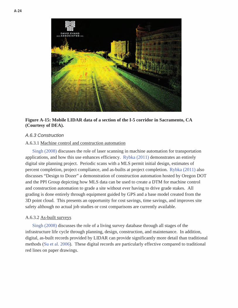
A-24

Figure A-15: Mobile LIDAR data of a section of the I-5 corridor in Sacramento, CA (Courtesy of DEA).

A.6.3 Construction

A.6.3.1 Machine control and construction automation

Singh (2008) discusses the role of laser scanning in machine automation for transportation applications, and how this use enhances efficiency. Rybka (2011) demonstrates an entirely digital site planning project. Periodic scans with a MLS permit initial design, estimates of percent completion, project compliance, and as-builts at project completion. Rybka (2011) also discusses “Design to Dozer” a demonstration of construction automation hosted by Oregon DOT and the PPI Group depicting how MLS data can be used to create a DTM for machine control and construction automation to grade a site without ever having to drive grade stakes. All grading is done entirely through equipment guided by GPS and a base model created from the 3D point cloud. This presents an opportunity for cost savings, time savings, and improves site safety although no actual job studies or cost comparisons are currently available.

A.6.3.2 As-built surveys

Singh (2008) discusses the role of a living survey database through all stages of the infrastructure life cycle through planning, design, construction, and maintenance. In addition, digital, as-built records provided by LIDAR can provide significantly more detail than traditional methods (Su et al. 2006). These digital records are particularly effective compared to traditional red lines on paper drawings.

A-25

A.6.3.3 Post construction quality control

In addition to providing high accuracy as-built records, MLS can provide quality control on the construction process. Tang et al. (2011) discuss the use of algorithms for determining the flatness of concrete, providing permanently documented results of the flatness defects and permitting users to remotely access the surface. Kim et al. (2008) verify super-elevation slopevalues, curb design, and soundproofing wall design by creating cross sections of a roadway at 5m intervals. The MLS data can then be compared to the original CAD drawings to ensure construction was completed within tolerance.

A.6.4 Operations

A.6.4.1 Traffic congestion

Traffic congestion typically results from human error, and automakers are researching methods to remove much of the human component from driving. BMW has been developing a system called Traffic Jam Assistant to take over driving tasks when vehicle speed is lower than 25 mph. The system relies on GPS and LIDAR along with other components to perform steering, braking, and acceleration (Barry 2011).

Thornton et al. (2012) used mobile LIDAR to evaluate parking utilization along arterial roads at various times of the day. They propose mounting MLS units on public vehicles such as buses, which could collect daily datasets along specific routes. They also noted the potential for vehicle classification and parking duration from the repeat datasets. Comparison of the automated approach to ground truth showed a small error rate of 1/340 vehicles.

A.6.5 Maintenance

Mobile LIDAR can also be used for maintenance purposes. Many maintenance tasks are similar to those described in Section A.6.3, Construction. Hence, the reader is referred to that section for more details. One key advantage is that mobile LIDAR could enable a rapid As-Built, geospatial record of maintenance that was completed, reducing the need for future, repeat surveys (Singh 2008).

A.6.5.1 Pavement analysis

The data collected for roadways can be used for several geometric analyses including stopping sight distances, adequate curve layouts, slope, super-elevation, drainage properties, lane width, and pavement wear. For instance, Zhang and Frey (2005) found that road grade could be reliably determined (within 5% compared to design drawing data) with airborne LIDAR data. Amadori (2011) found that mobile LIDAR can be an effective tool for cross slope determinations, particularly when identifying sections that are out of compliance. Several pavement resurfacing vendors have found the data to be effective to reduce change orders and over-run costs for resurfacing projects.

A-26

Herr (2010) presents several examples of how MLS data can be used to evaluate pavement condition including rutting, ride quality, rehabilitation, texture, and automated distress. He emphasizes that the acquisition of all of these data from a single, integrated point cloud represents a major paradigm shift for the industry where these data are acquired from a variety of sources. Tsai and Li (2012) document controlled laboratory tests using laser profiling units to scan pavement at high detail at ambient lighting and low intensity contrast. The system was effective in detecting cracks automatically; although scanner tilt angle, transverse profile spacing, and sampling frequency were key variables influencing the detection accuracy.

Chang et al. (2006) performed tests to compare the use of static 3D laser scanning, Multiple Laser Profiler (MLP), and rod and level surveys and found significant correlation (99%). As MLS accuracies increase, it may provide the ability to provide detailed surface roughness data, which are important to evaluate new pavement smoothness quality, resulting in significant incentives and disincentives for contractors. Chin and Olsen (2011) have shown that static TLS data has potential for pavement smoothness evaluation, which determines significant financial incentives/disincentives for contractors on highway construction projects. Potentially, scanner intensity information could be usable to determine the reflectivity of painted stripes, signs, and more. (However, actual implementation requires continued research and development to appropriately normalize intensity values). Scanner intensity information can also be used to highlight damaged sections of concrete (Figure A-16) or asphalt pavement, which reflects light differently.

Figure A-16: Intensity return used to highlight concrete cracking in a static scan (plan view).

A-27

A.6.6 Safety

State DOTs are required to submit Highway Performance Management System (HPMS) reports. Many elements needed (e.g., road geometry) for this report can be acquired efficiently through a mobile LIDAR system (particularly when additional sensors are mounted to the vehicle).

AASHTO’s Highway Safety Manual (HSM) includes algorithms that have been developed into SafetyAnalyst (network level) and the Interactive Highway Safety Design Model (IHSDM, project level). Both of these input roadway data and provide safety evaluations such as expected crash rates. Many of these inputs are geometric and can be captured with mobile LIDAR.

A.6.6.1 Extraction of features for safety analyses

Lato et al. (2009) demonstrate how rock fall hazards along transportation corridors can be monitored using MLS. For this study, the monitoring took place from both railway and roadway based MLS systems. In both situations, MLS provided increased efficiency and also the ability to monitor hazards in real-time. The safety benefits from real-time monitoring also extend beyond locating unstable rock hazards.

A.6.6.2 Accident investigation

TLS systems have been used to document accident scenes, permitting the accidents to be moved off the roadway sooner, and allowing investigators to continue the investigation after all physical evidence has been removed from the scene. 3D Laser Mapping (2011) reports that accident scene investigation can be 50% faster than total station surveying, resulting in a 1.5 hour reduction in roadway closure. According to Duffell and Rudrum (2005) and Mettenleiter et al. (2008), MLS has begun to play an important role in documenting pre-accident conditions, and also, a much faster means of documenting long accident scenes which typically occur in high speed crashes. Jacobs (2005) discusses that laser scanning may also be used to analyze structural damage caused by vehicular impact on bridge overpasses due to vehicle height exceeding the bridge clearance.

MLS systems can rapidly scan networks of tunnels for damage inspection. Rapid deformation analysis enables highway crews to safely open a tunnel soon after a problem is resolved. However, the resulting accuracy using MLS will depend heavily on the length of the tunnel and quality of the IMU because GNSS data will not be available in the tunnel. Figure A-17 shows an example of an intensity-shaded TLS dataset obtained for a tunnel damaged by fire. Oregon DOT is planning to use their mobile LIDAR system to scan tunnels in Oregon on a repeat basis for monitoring.

A-28

Figure A-17: Close examination of the intensity-shaded point cloud (static scan) shows additional, minor damage to concrete in a tunnel in Oregon. (Courtesy of Oregon DOT).

A.6.6.3 Driver assistance/autonomous navigation

Brenner (2009) and Toth (2009) discuss how MMS’s have begun to shape the research track of the autonomous vehicle navigation field. Toth (2009) predicts that autonomous vehicle navigation could be operational within the next decade. Brenner (2009) tests a simulated car, designed to model what a fully autonomous vehicle would be able to sense from a position on the roadway. This is done by automatically extracting poles (any vertical narrow structure), and then allowing the autonomous vehicle to calculate positioning based on the constellation of the poles. Pole extraction is performed on an already geo-referenced point cloud, and vehicle positioning calculated along the roadway based on referencing to the located poles. Kodagoda et al. (2006) describe how laser systems on vehicles can be used to track curbs.

A.6.7 Research

A.6.7.1 Unstable slopes, landslide assessment

Su et al. (2006) describes the use of LIDAR data for geotechnical monitoring of excavations, particularly in urban areas. In these urban excavations, real-time monitoring of the excavation site as well as surrounding infrastructure is critical in maintaining integrity. Miller et al. (2008) demonstrate the use of TLS in assessing the risk of slope instability, and provide two examples along transportation corridors. The authors note the challenge and safety issues that arise from setting up a stationary TLS instrument along the side of a busy transportation corridor. Figure A-18 demonstrates how LIDAR can be used to highlight localized slope failures. Olsen et al. (2011b) developed an algorithm that permits in-situ detection of changes that have occurred over a region of previously collected LIDAR data using static LIDAR. This allows field crews to

A-29

immediately see where changes have taken place so that any additional measurements can be made at the site with no need for office processing of the point cloud. Although mobile LIDAR data is not often processed in real time, it can provide baseline information for such a framework.

Figure A-18: Static scan of a surficial slope failure along highway embankment at the US 20 Pioneer Mountain to Eddyville re-alignment project in Oregon. (Note that the failure scarp is covered by a white tarp to prevent sediment from entering nearby water).

Lato et al. (2009) found that mobile LIDAR was advantageous compared to static LIDAR in coverage, acquisition rate, and corridor operation integration. Mobile LIDAR provided slope heights, angles, and profiles. Using a rail mounted mobile LIDAR system, 20km of railway were acquired in 5 hours producing a 15 GB dataset with accuracies of 15 cm (absolute) and 5 cm (relative). Figures A-19 and A-20 demonstrate similar use of LIDAR along unstable slopes for Oregon DOT and Alaska DOT to evaluate slope stability.

Although based on static scanning research, a pooled fund study conducted recently evaluated the use of LIDAR to map geotechnical conditions of unstable slopes, including rock mass characterization, surficial slope stability, rockfall analyses, and displacement monitoring. The report (soon to be released) provides an overview of ground-based LIDAR and processing software, discusses how LIDAR can be integrated into geotechnical studies, and includes case studies in the states of Arizona, California, Colorado (two sites), New Hampshire, New York,

A-30

Pennsylvania, Tennessee, and Texas. The authors also discuss best practices and procedures for data acquisition to ensure it provides reliable data for geotechnical analyses (Kemeny, Combs,

Figure A-19: Point cloud of a rockfall on newly cut section for a highway. (Courtesy of Oregon DOT).

Figure A-20: Point cloud for MLS data obtained for slope stability assessment on the Parks Highway near Denali National Park, Alaska.

R

Cut Slope

Road (Undeer Construction)

Lanndslide

Cut Slope

et al., unpublished work).

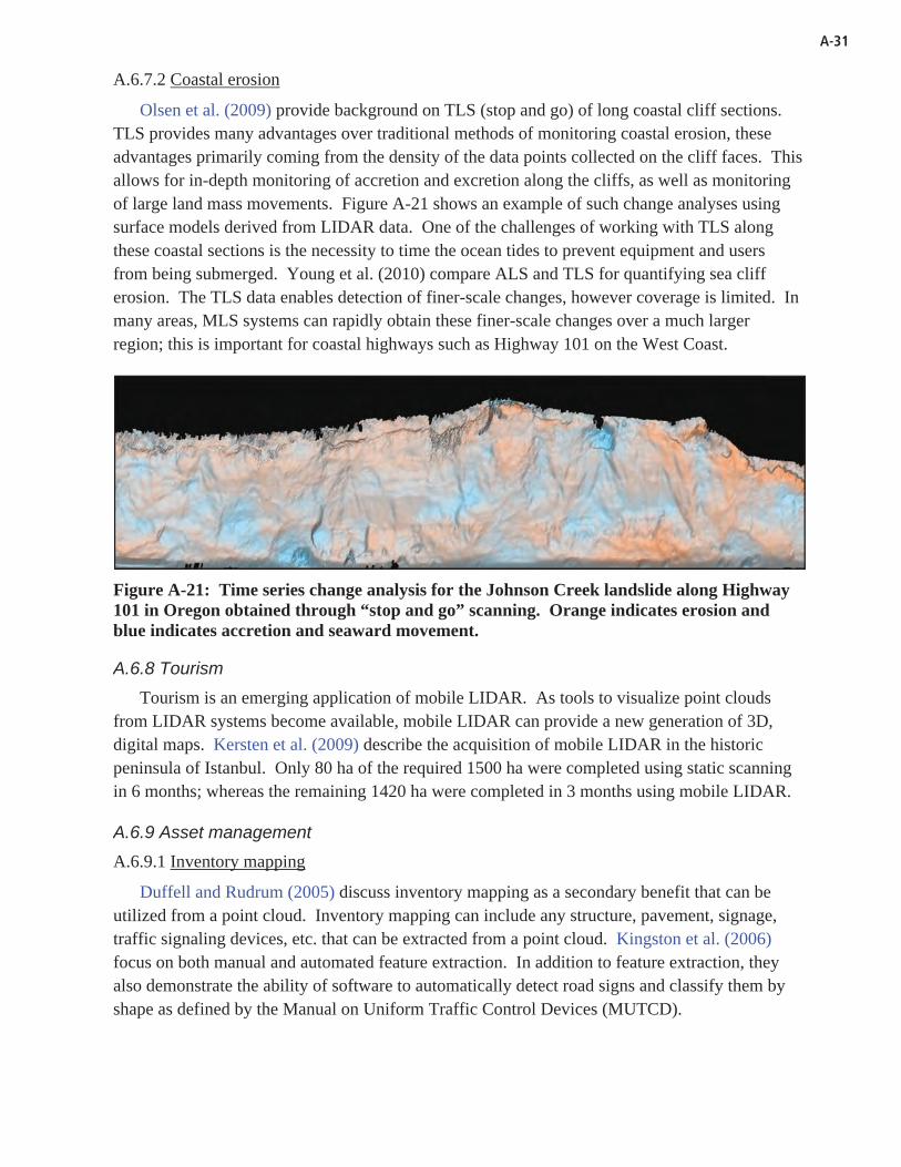
A-31

A.6.7.2 Coastal erosion

Olsen et al. (2009) provide background on TLS (stop and go) of long coastal cliff sections. TLS provides many advantages over traditional methods of monitoring coastal erosion, these advantages primarily coming from the density of the data points collected on the cliff faces. This allows for in-depth monitoring of accretion and excretion along the cliffs, as well as monitoring of large land mass movements. Figure A-21 shows an example of such change analyses using surface models derived from LIDAR data. One of the challenges of working with TLS along these coastal sections is the necessity to time the ocean tides to prevent equipment and users from being submerged. Young et al. (2010) compare ALS and TLS for quantifying sea cliff erosion. The TLS data enables detection of finer-scale changes, however coverage is limited. In many areas, MLS systems can rapidly obtain these finer-scale changes over a much larger region; this is important for coastal highways such as Highway 101 on the West Coast.

Figure A-21: Time series change analysis for the Johnson Creek landslide along Highway 101 in Oregon obtained through “stop and go” scanning. Orange indicates erosion and blue indicates accretion and seaward movement.

A.6.8 Tourism

Tourism is an emerging application of mobile LIDAR. As tools to visualize point clouds from LIDAR systems become available, mobile LIDAR can provide a new generation of 3D, digital maps. Kersten et al. (2009) describe the acquisition of mobile LIDAR in the historic peninsula of Istanbul. Only 80 ha of the required 1500 ha were completed using static scanning in 6 months; whereas the remaining 1420 ha were completed in 3 months using mobile LIDAR.

A.6.9 Asset management

A.6.9.1 Inventory mapping

Duffell and Rudrum (2005) discuss inventory mapping as a secondary benefit that can be utilized from a point cloud. Inventory mapping can include any structure, pavement, signage, traffic signaling devices, etc. that can be extracted from a point cloud. Kingston et al. (2006) focus on both manual and automated feature extraction. In addition to feature extraction, they also demonstrate the ability of software to automatically detect road signs and classify them by shape as defined by the Manual on Uniform Traffic Control Devices (MUTCD).

A-32

A.6.9.2 Modeling and inspection

Becker and Haala (2007) emphasize the need for detailed 3D modeling of urban landscapes for city planning. They demonstrate an automated façade grammar building tool that can model building facades beyond the line of sight of the scanner by hypothesizing further facades based on the adjoining style. Jochem et al. (2011) also proposes using MLS to model building facades; however, the focus is to select the facades with the highest solar potential. The goal is to extract individual structures from a point cloud and assign solar potential ratings to the various facades of the structure. This would allow individuals to easily see where the most appropriate placement for solar panels would be on their building.

A.6.9.3 Automated/semi-automated extraction of features

New algorithms are under development to extract features in a point cloud. Many of these are currently semi-automatic and require significant user verification of results. However, many researchers are developing robust, fully automated feature extraction tools. For example, although primarily developed for robotics, the Point Cloud Library (PCL, http://pointclouds.org/) is a recent open source resource that has libraries for feature extraction from point clouds of geometric primitives (planes, cylinders, etc.). Common features extracted from point cloud data include signs, streetlights\poles, reflective striping, and curbs. Please note that many of these procedures currently have only been tested on limited, test datasets and have not been integrated into mainstream software. However, current software is rapidly evolving to implement these novel techniques.

McQuat (2011) discusses several different structures (signs, facades, bays, automobiles, curbs, et al.) including how they can be automatically detected and converted to useful shapes for use in a GIS.

Pu et al. (2011) describe automated algorithms to recognize features within a point cloud such as traffic signs, trees, building walls, and barriers using characteristics such as size, shape, orientation, and topological relationships to classify the point cloud. The authors indicate that poles are recognized with an accuracy of 86%; however, other categories were not extracted as successfully and need to be integrated with imagery for extraction.

Semi-automatic or fully automatic extraction of signs is necessary to efficiently locate signs in a large point cloud such as that provided by MLS. Figure A-22 provides an example of how the intensity values of the scanner can be used to identify reflective signage, which can be semi-automatically detected for extraction and cataloging.

Novak (2011) discusses the use of MLS to extract streetlights in El Paso, TX, and store them in a database managing light bulb replacement. Due to an increase in worker safety and a faster rate of completion, MLS was chosen for the project. Brenner (2009) discusses a method of pole extraction by use of cylindrical stacks; these stacks contain a core that must contain data

A-33

surrounded by a ring that contains no data. Lehtomaki et al. (2011) used MLS data to extract poles and trees. The automated method successfully detected 70% of the poles and 78% of the trees at two field sites. Of the detected features, 81% (poles) and 87% (trees) were correctly identified. The algorithm had difficulty recognizing tree trunks surrounded by branches and wall structures.

Rutzinger (2009) combine airborne and mobile LIDAR data to extract vertical walls for building facades. These wall faces are then used to correct building outlines in cadastral map data. Following point cloud segmentation through a region grow process, individual points are classified based on planarity, inclination, wall height and width. Upon detection of a vertical wall, the MLS points are then compared to the vertical wall from the cadastral map to estimate the potential completion of the MLS data. Vegetation, for example, created several occlusions.

Alabama DOT also recently implemented mobile LIDAR for maintaining a billboard inventory and found it to be a cost-effective system.

Lin and Hyyppa (2010) developed an automatic methodology to detect pedestrian culverts from DTMs created from mobile LIDAR data. Because of limited view of the culverts from the roadway, culverts could only partially be characterized. However, calculated lengths and widths of the culverts were within 9% and 16% of actual measurements.

Figure A-22: Reflective signs (red) extracted from a static TLS point cloud at the Oregon State University campus.

A-34

A.7 DATA QUALITY CONTROL

A.7.1 Accuracy and precision checks

Each component of the MLS setup requires careful calibration to ensure accurate data. Calibration errors are additive in the scanning platform; each portion of the system that is not well calibrated propagates errors to the final point cloud.

A.7.1.1 Laser scanning errors

System specification sheets provide a basic idea of scanner performance; however, additional factors need to be considered that are well beyond the scope of the specification sheet. Also, because standardized testing procedures have not been developed, it can be difficult to directly compare values from one system to another. Error sources include the material properties of the scanned objects, environmental conditions, inconsistencies in scanner manufacturing, the geometric configuration of the object to the scanner, and GPS errors.

• Material Properties: White surfaces will provide very intense laser returns, while black surfaces will return a much less intense value (Boehler et al. 2003). System performance varies greatly, and consideration needs to be taken for the objects being scanned, such as low reflectivity asphalt in many transportation applications. Highly reflective surfaces (e.g., traffic signs, retro-reflectors) may produce additional distortion effects such as saturation and blooming (Vosselman and Maas 2010). Saturation (Figure A-23) is caused by too much energy being returned to the scanner and appears as points spread out along the line of sight of the scanner. Blooming (Figure A-24) is a similar effect that occurs perpendicular to the line of sight of the scanner, creating an apparent enlargement of the reflective surface due to excessive energy being returned to the scanner.

Figure A-23: Extreme case of Saturation of a flat, 5cm retro-reflective target (red) is seen as the target extending 4cm off of the wall. Left: Straight on view (down on Y-axis). Right: side view along plane of wall that target is affixed to (along X-axis).

Wall

Target

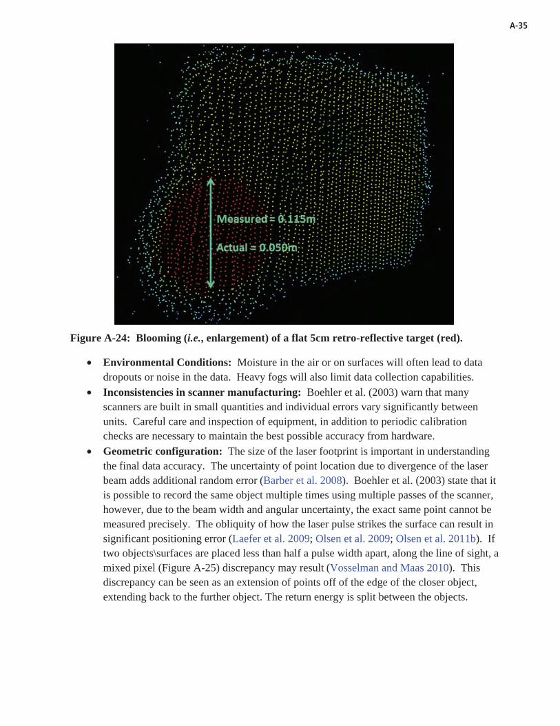
A-35

Figure A-24: Blooming (i.e., enlargement) of a flat 5cm retro-reflective target (red).

• Environmental Conditions: Moisture in the air or on surfaces will often lead to data dropouts or noise in the data. Heavy fogs will also limit data collection capabilities.

• Inconsistencies in scanner manufacturing: Boehler et al. (2003) warn that many scanners are built in small quantities and individual errors vary significantly between units. Careful care and inspection of equipment, in addition to periodic calibration checks are necessary to maintain the best possible accuracy from hardware.

• Geometric configuration: The size of the laser footprint is important in understanding the final data accuracy. The uncertainty of point location due to divergence of the laser beam adds additional random error (Barber et al. 2008). Boehler et al. (2003) state that it is possible to record the same object multiple times using multiple passes of the scanner, however, due to the beam width and angular uncertainty, the exact same point cannot be measured precisely. The obliquity of how the laser pulse strikes the surface can result in significant positioning error (Laefer et al. 2009; Olsen et al. 2009; Olsen et al. 2011b). If two objects\surfaces are placed less than half a pulse width apart, along the line of sight, a mixed pixel (Figure A-25) discrepancy may result (Vosselman and Maas 2010). This discrepancy can be seen as an extension of points off of the edge of the closer object, extending back to the further object. The return energy is split between the objects.

A-36

Figure A-25: Mixed pixels appear in an area occluded from the scanner’s line of sight.

• GPS source errors: Factors that affect the accuracy of GPS include: multipath, shading by buildings and trees, loss of satellite lock, atmospheric conditions, and poor satellite geometry (Glennie 2007b and Haala et al. 2008). GNSS systems combining GPS, GLONASS, Galileo, and Compass (when available) will help improve accuracy results (Chiang et al. 2010).

A.7.2 Procedures for measurement quality control

Many different methods have been employed to verify the accuracy of the final point cloud. Commonly, ground control points, or an already geo-referenced TLS point cloud are used to verify accuracy of the MLS data. Ussyshkin (2009) discusses geo-referencing mobile scan data using a system of six base stations and ground control points spaced every 50-80 meters throughout the survey extents in order to achieve 1-2cm accuracy. While this may be achievable for a small project, a MLS survey needed for a system-wide analysis could not be economically completed with this amount of control required. Caltrans specifications call for these validation points every 500ft ( ~152m). Barber et al. (2008) state automated validation to compare MLS data to survey control high resolution terrestrial laser scans, or target matching in real-time is greatly needed. Hiremagalur et al. (2007) provide “best practices” to ensure the proper registration of MLS data and recommend target redundancy (if target registration is to be used), examination of overlapping point clouds, and comparison of point cloud coordinates to check point coordinates surveyed using traditional methods. A report of the RMS error of the point cloud to the ground control coordinates should be a standard deliverable in addition to an RMS error report of overlapping point clouds. Points to be used for an RMS evaluation should be spatially distributed throughout the entire dataset. Additionally, Graham (2010) recommends

A-37

that final quality control be performed by someone other than those involved in registering the dataset.

A.7.3 Data collection categories concept

When assessing the quality of a mobile mapping system point cloud, many factors contribute to the final accuracy and precision values. Boehler et al. (2003) describe that various jobs will require various levels of data quality. The ASPRS Mobile Mapping Committee (2011) and Hiremagalur et al. (2007) have recommended that final point cloud quality be assigned a rating based on the quality of data. For example, an end user may be in need of a point cloud to inventory roadway signs along a corridor. The user may not be concerned with the geo-referencing accuracy of these signs; they may be using the data solely for the purpose of counting the number of signs along the corridor. In this example, the user would not want to pay a premium for survey quality positional data, which also requires additional field time to complete. This user still needs high enough resolution in the point cloud to be able to reliably extract the signs.

This creates a two-fold level requirement for the data in that it needs to address both the accuracy and the resolution of the data (ASPRS Mobile Mapping Committee 2011). Accuracy tends to have a higher impact on project cost, since higher resolution can be more easily obtained with slower vehicle speeds, or multiple passes through the corridor. According to Barber et al. (2008), positioning is not affected by vehicle speed; whereas, higher speeds lead to lower point density.

However, Duffell and Rudrum (2005) argue that the over-collection of data may not always be a negative, because data can often be reused for many different tasks. One data cloud could be made available to many end users who can mine the data source for several different job tasks. In addition, extra detail could allow the reuse of archived point clouds for base data in accident investigations, hazard identification, and future project planning.

A.8 CURRENT CHALLENGES

Several difficulties exist when performing mobile scans (e.g., Glennie 2009b). Measurements are performed from a moving platform, requiring high precision GPS/IMU readings for accurate data geo-referencing. Typically it is not feasible to close down a section of highway for scanning, so neighboring vehicles can block data collection efforts. Additionally, the vehicle must be moving at a safe speed (with the flow of traffic) while simultaneously collecting data. In some cases, a rolling slow down can be used to avoid these problems.

Further, the size and complexity of the laser scan data presents significant challenges. Sensors collect data at very high speeds (typically 100k to 1 million points per second) and at very high point densities (typically >100 points per m2) at close ranges (typically < 100m). This creates large datasets that can be difficult to work with on typical computing platforms and

A-38

software. The volume of data collected also requires a substantial amount of data storage and backup during a project.

Following completion of a project, care must be taken to ensure proper data archival. The large size also makes web, DVD, or other common media difficult to use for data transfer or sharing both within an agency and with external partners. The complexity of data and minimal availability of software also presents challenges to end users such as transportation agencies in actually being able to use the data. Ussyshkin (2009) discusses limitations on the number of points that can be imported into common software packages. Currently, many consultants subsample and filter the data to reduce size. They also process the data in small sections (tiles) because computing resources limit their ability to work with the entire dataset. Often, the final data typically transferred to the end user may only represent a fraction of the original data obtained. In several cases, the actual point cloud is not being delivered.

While manufacturers of GIS and CAD software have recently been integrating point cloud support, many challenges remain to make this process seamless for the end user. Further, point cloud processing usually requires working between multiple software packages where information can be lost on imports and exports through the process. The ASTM E57.04 (2010) subcommittee on data interoperability was formed, in part, to help resolve these data transfer issues. In addition, working with a 3D point cloud requires skill to ensure that appropriate measurements are extracted.

Knaak (2012b), after a conversation with Florida DOT personnel, discusses problems with MLS technology adoption by transportation agencies and offers suggestions including:

1. Avoid the “WOW” factor of point clouds. Often this results in incomplete projects where consultants do not provide transportation agencies with something they can actually use,

2. Agree on a QA/QC procedure, including a lineage from the point cloud to the final product and metrics to evaluate that lineage. The QA/QC should be done by an independent contractor,

3. Identify the model needs first so that the point cloud requirements can be determined easier, and

4. Define the respective responsibilities of the customer and consultant in the process.

Knaak (2012b) also explains problems in current payment and procurement standards that are focused on time in field work and minimal office processing time. The key factor with MLS technology is that it reduces field time dramatically (80-90%) but shifts loads to processing. Under current payment schemes, these current payment schemes reduce the contractors’ pay substantially because they are paid based on field time.

A-39

A.9 BEST PRACTICES AND LESSON LEARNED

Unfortunately, many of the lessons learned and user experiences are being disseminated verbally at conferences or other events, but currently have not been adequately integrated into retrievable documents. Many service providers are also reluctant to document and make project reports available because of liability concerns.

Missouri DOT (Vincent and Ecker 2010) evaluated the accuracy, cost and feasibility of airborne, mobile, and static terrestrial laser scanning for typical transportation projects. They determined that all systems met their accuracy requirements. The report also highlights current hurdles including software and computing challenges. The authors also conclude that traditional surveying and/or static scanning may still be required to fill in gaps from mobile scanning.

Yen et al. (2011) provide an in-depth evaluation of MLS technology in the State of Washington. They show that maintenance, asset management, engineering, and construction programs all incur cost savings, time savings, and safety improvements with MLS. This evaluation also demonstrates the needs of national standards and best practices as well as a common data exchange platform to improve data interoperability.

Singh et al. (2012) present an overview of theory applied to mobile LIDAR and practical implementation for a case study of an 8 mile segment of the I-5 corridor. This workshop presentation discusses project planning, quality management plans, data acquisition, data processing, deliverables and lessons learned. Lessons learned include placing pre-marks (control points) on both sides of the run, providing significant overlap between cloud strips, breaking runs into manageable segments, planning for acquisition on lengths much larger than originally anticipated to cover frontage roads and ramps, and having flexible data storage and transfer mechanisms.

Many lessons learned have not yet been formally documented with rigorous testing results. However, there are often “nuggets of wisdom” that can be found on various websites. For example, many service providers and vendors publish short articles of projects and experiences on http:\\lidarnews.com. Some service providers regularly update a blog, such as Michael Baker Jr. Inc. (http://mobilelidar.blogspot.com). As an example, this blog includes a discussion of “lessons learned” from their experiences. Below is an excerpt:

“Baker's Dozen: 13 Laws of Mobile LIDAR (also currently being chiseled on a slab of granite):

1. Too much is better than not enough. 2. Sometimes more is just more, not better. 3. Hard drives are cheap, time isn’t. 4. Consistency counts; stop guessing. 5. When someone wants “full planimetrics,” they really don’t.

A-40

6. The stated laser range is X’, but the lasers are only capturing data to Y’; and Y is definitely less than X, yet nobody can tell you what Y is…

7. The data you capture is only as good as the applied control. 8. Today’s best practices will be tomorrow’s old habits. 9. Field vs. office time ratios are pipe dreams. 10. Mobile LIDAR systems are not created equal, and neither are the operations behind them. 11. Off-the-shelf processing software will only do 50% of what you need it to do. 12. When the system encounters issues, take a breath and reboot. 13. Mobile LIDAR is not all fun and games, but it does feel like it some days.”

Siebern (2012) presents two case studies and information on “managing expectations for mobile mapping solutions,” from the perspective of a service provider. Particularly, the author mentions that proper communication and understanding between service providers and clients is critical to project success, particularly related to the fact that the LIDAR industry is evolving. The case studies (interstate corridor design and overhead catenary system) discuss various aspects of the projects including expectations, deliverables, challenges, and unforeseen benefits (e.g., usefulness of the imagery for other purposes than originally intended) associated with the projects.

Recently, Chang et al. (2012) through a questionnaire and literature review documented several important lessons learned for various transportation agencies, including:

1. Despite benefits of LIDAR, it is not a complete substitute for traditional surveying. 2. Due to technical difficulties with hardware and software, a trained technician is required

for editing and extraction, which can be a costly investment to implement. 3. Specifications need to be clear, particularly with accuracy requirements regardless of

whether it is in-house surveyors or third-party contractors.

Burns and Jones (2012) reported on the recent U-Plan project to collect mobile LIDAR data for all roads within the state managed by the DOT. Key lessons learned include:

1. Ensure the DOT has the ability to store, distribute, analyze and utilize the data collected. 2. Build support from senior management. 3. Prepare for potential lengthy procurement processes. 4. Be prepared to work extensively with the vendor from selection to final data collection.

For example, they found that a weekly meeting with the data provider was beneficial to the project, and

5. Do not expect to fund your entire data wish list up front!

A-41

A.10 EXISTING GUIDELINES

Many agencies (FAA 2011; FGDC, 1998; NDEP 2004; NOAA 2009; USGS 2012) have provided recommendations, guidelines, or standards for geospatial data. Some of these (FGDC, 1998 and NDEP 2004) are broad specifications that pertain to all remotely sensed data while others pertain more directly to LIDAR data (FAA 2011; NOAA 2009; USGS 2010). The ASPRS has produced “ASPRS Guidelines: Vertical Accuracy Reporting for LIDAR Data” (ASPRS 2004) and “(DRAFT) ASPRS LIDAR Guidelines: Horizontal Accuracy Reporting” (ASPRS 2005), which more specifically declare reporting standards (e.g., fundamental vertical accuracy (FVA), consolidated vertical accuracy (CVA), supplemental vertical accuracy (SVA)). A summary of these guidelines can be seen in Table A-1.

Common trends can be seen in the various LIDAR specifications, including:

1. Standard accuracy reporting methods, 2. Requirements for ground point density, 3. Requirements for scan overlap, 4. Number and distribution of control/check points for accuracy verification, and 5. Types of deliverables.

Although most of these guidelines are currently focused on aspects of ALS, some of their

fundamental principles can be adapted to produce guidelines more relevant to mobile LIDAR. However, most of these documents do not directly or adequately address the needs of many transportation applications. For example, the accuracy, resolution, coverage, and look angle of mobile LIDAR data varies significantly from that achieved with airborne LIDAR. Particularly, true 3D error vectors are important for many applications that cannot be evaluated by focusing on vertical error only.

A.10.1 Geosptial Data Accuracy

The Federal Geographic Data Committee (1998) developed the National Standard for Spatial Data Accuracy (NSSDA), which provides guidance on reporting spatial data accuracies. This document provides the foundation for the reporting found in most available standards and guidelines. The NSSDA uses a root mean square error (RMSE) to estimate positional accuracy reported in ground distances at 95% confidence. Datasets should be tested with a minimum of 20 control points and reported as:

Tested ____ (meters, feet) vertical (or horizontal) accuracy at 95% confidence level

In cases were the data were not tested and accuracy is merely estimated, the following statement is used:

Compiled to meet ____ (meters, feet) vertical (or horizontal) accuracy at 95% confidence level

A-42

The National Digital Elevation Plan (NDEP) guidelines further developed the NSSDA to include three types of accuracy reporting: fundamental vertical accuracy (FVA, open terrain, optimal conditions), consolidated vertical accuracy (CVA, combined accuracies obtained in all land covers), and supplemental vertical accuracy (SVA, accuracies reported for individual land covers). For example, accuracies in dense forests will be much less than in open terrain.

Table A-1: Summary of existing LIDAR guidelines.

General Geospatial Key PointsFederal Geographic Data Committee (FGDC) 1996 National Standard for Spatial Data Accuracy (NSSDA)

95% confidence evaluation, 20 control points, methodology on how to compute accuracy statistics

National Digital Elevation Plan (NDEP) 2004

DTM certification, reporting of accuracy across many different remote sensing platforms. Discusses Fundamental, Supplemental, and Consolidated Vertical Accuracies (FVA, SVA, CVA)

Mobile LiDAR (Current)

CALTRANS Chapt. 15 Survey Manual 2011 Florida DOT 2012

TLS and MLS specifications, various classes of data (Type A-high accuracy, Type B-lower accuracy), requirements for: mission planning, control placement, system calibration, overlap requirements, QA/QC

Mobile LiDAR (Development)TxDOT In developmentASPRS Mobile Mapping Committee At outline stageMoDOT 2010 Evaluation of MLS usage for DOT activities

Airborne LiDAR

FAA 2011Includes LIDAR (airborne, static, and Mobile) standardsand recommended practices for airport surveys. System calibrations, data processing.

NOAA 2009 Use of LIDAR for shoreline and flood mapping.

USGS (2012)V1.0. Base Specification. Post spacing, overlap requirements, classification, metadata example, DEM., vertical accuracy assessment, glossary of terms.

ASPRS VerticalApplying FGDC and NDEP guidelines to airborne LIDAR. Land cover types. Selection of checkpoints.

ASPRS HorizontalConsiderations (and difficulty) of horizontal accuracy verification.

ASPRS Geospatial Procurement GuidelinesDraft phase. Distinguishes between professional/technical services and commercial geospatial products.

FEMA Guidelines LIDAR use in floodplain mapping.

Existing Guidelines

A-43

A.10.2 ASPRS guidelines

The American Society of Photogrammetry and Remote Sensing (ASPRS) is striving to be the go-to source for LIDAR technology in the US. Several efforts are underway, including:

• The ASPRS Mobile Mapping Committee is developing guidelines for mobile mapping. This is currently a work in progress at the outline stage.

• ASPRS Vertical accuracy guidelines for airborne LIDAR. This document reinforces the NSSDA and NDEP guidelines and provides guidance for establishing control specific to airborne LIDAR.

• ASPRS horizontal accuracy guidelines for airborne LIDAR. This document provides background on the difficulties in determining horizontal accuracies from airborne LIDAR.

• ASPRS Geospatial Procurements (DRAFT). This document is intended to aide entities with the best approach to commercial geospatial products, defined with a COTS specification. The document distinguishes between professional\technical services and commercial geospatial products. It also recognizes state and federal laws. A proposed procurement methodology of license data terms and conditions, cost/value, service provider defined technical specification, services to support geospatial products and deliverables are addressed. ASPRS also previously produced procurement guidelines for geospatial mapping services.

A.10.3 Transportation agency LIDAR standards

Chapter 15 of the California Department of Transportation (2011) Surveys Manual is one of the first developed sets of specifications that explicitly addresses the required information and data quality that should be provided with static and mobile LIDAR surveys. These specifications contain a two part classification system for mobile LIDAR surveys. Type ‘A’ is a higher accuracy, hard surface survey used for engineering applications and forensic surveys. Type ‘B’ is used for lower accuracy earthwork measurements (e.g., asset inventory, erosion, environmental and earthwork surveys).

These specifications are broad enough to not limit service provider equipment and technology but provide details regarding data acquisition and processing procedures, including the minimum overlap between scans, maximum PDOP, minimum number of satellites, maximum baseline, validation point accuracy requirement, IMU drift errors, and other factors pertaining to the geo-referencing accuracy of the point cloud. However, one needs to have a relatively high level of understanding of mobile LIDAR technology in order to utilize these aspects of the Caltrans standards effectively.

Other transportation agencies have begun developing standards and guidelines for MLS. These Guidelines are meant to provide the agency with a reference document that can be tailored to their specific needs. For example, Florida DOT recently released guidelines which are very

A-44

similar to the Caltrans guidelines. However, the Florida DOT guidelines add a Type C, Lower Accuracy Mapping category for planning, transportation statistics, and general asset inventory surveys.

A.10.4 FAA Advisory Circular

The Federal Aviation Administration has produced a draft Advisory Circular related to remote sensing technologies. This document includes a section which discusses considerations for use of several forms of LIDAR (static, mobile, and airborne) for airport surveys and anticipated accuracies and resolutions for each method. The document also discusses calibration procedures for LIDAR systems and provides guidance when such calibrations are necessary. Specific requirements for mobile LIDAR workflows include: redundancy, monitoring acquisition, local transformation and validation points, data processing, data filtering and clean up, geo-referencing, and data integration.

A.10.5 Industry Guidelines

Some service providers have developed guidelines for transportation agencies that they have worked with. Many of these are not published and can differ by transportation agency, to meet their individual needs. For example, Knaak (2012a) has developed a set of best practices based on experience; this document defines three distinct levels of data as well as requirements for: vehicle trajectory, point cloud, file management, and images.

A.11 MOTIVATION AND KEY NEEDS FOR NATIONAL GUIDELINES

Mobile LIDAR data provides many benefits when processed and used appropriately. Ussyshkin (2009) states that the underlying technical details (e.g., applications, procedures, benefits) need to be well understood in order to prevent disappointments and misunderstandings when using mobile LIDAR data. Guidelines need to incorporate and integrate fundamental principles of quality control and performance to result in the desired deliverable. Optimally, end users such as engineers and designers should have a strong understanding of mobile LIDAR, so that the data can be utilized effectively and to its full potential. However, because of the wide variety of applications and quality needs, many personnel within a transportation agency can effectively use mobile LIDAR without being experts in the details of the technology once the appropriate guidelines are in place. Simple, yet powerful, guidelines focused on performance evaluation will enable them to adequately integrate mobile LIDAR into their operations. National guidelines will ensure that transportation agencies do not duplicate efforts in producing similar documentation. The consistency provided through national guidelines will also enable improved communication between service providers and transportation agencies.

A-45

A.12 CONCLUSIONS

This literature review highlights the use of mobile LIDAR in transportation, including a discussion of current and emerging applications, data quality control, existing guidelines, and challenges. The review shows that there is a lot of interest for mobile LIDAR in transportation, provided appropriate guidance is in place.

From this review, there is a lot of discussion of WHAT is being done, but not a lot of HOW and HOW WELL it is being done. Generally, most information related to MLS use is from presentations at conferences or short web articles that do not go into detail regarding the work performed. Most quality control checks that are discussed in these reports are verified for vertical accuracy only. Very limited research exists to understand fully the capabilities and limitations of these systems.

Given the limited amount of experience that has been documented in the literature, to date it is important that future demonstration/pilot projects be adequately documented and the results disseminated both within a transportation agency and between agencies regarding the challenges, successes, and lessons learned from projects incorporating mobile LIDAR.

The literature review, in conjunction with the transportation agency questionnaire, reveals that there is a strong transportation agency\industry desire for:

• Standardized accuracy reporting methods • Data interoperability and management • Control/check requirements and procedures • Better understanding the data quality needs of specific applications (e.g., asset

management vs. engineering needs)

Another important consideration is that MLS is a tool in the transportation agency’s toolbox; sometimes it may be the best tool for a job, sometimes not. Hence, it is important that agencies understand when to and not to use mobile LIDAR.

B-1

A p p e n d i x B

Questionnaire Report

B.1 SUMMARY

The relatively recent emergence of mobile Light Detection and Ranging (LIDAR) technologies as a potentially transformative tool for numerous transportation engineering applications coupled with a lack of existing standards has resulted in the need for an improved understanding of how this technology is currently being implemented, and what challenges are limiting its adoption. To that end, a web-based questionnaire was administered to State Departments of Transportation (DOTs) in November 2011 to document and evaluate the state-of-the-practice regarding mobile LIDAR in transportation applications. Representatives from each of the 50 U.S. states and 6 additional transportation agencies completed the questionnaire, for a total of 74 responses. Multiple responses were obtained from a few DOTs, which allowed the team to capture variances between divisions within those DOTs.

This questionnaire provided the Project Team with the data needed to establish a technology adoption baseline for the DOTs by documenting current practices related to mobile LIDAR (also known as mobile laser scanning) use, guidance, and needs.

A second Service Provider Questionnaire was completed by 14 companies experienced with mobile LIDAR services and was administered via telephone interviews. The objective of this questionnaire was to provide additional perspective on the extent of use, and the challenges of adopting mobile LIDAR scanning by the DOTs from a service provider’s perspective. Given the much smaller sample sizes of the service providers, the intent is not to directly compare DOT and service provider perspectives but to provide an outside perspective.

Results from the DOT Questionnaire indicate that most agencies have experience with static laser scanning, with approximately 70 % having reported use of the technology for a project in the last 12 months. Most DOTs have also investigated mobile LIDAR to at least some degree and are excited about its potential use in the future. Approximately 50% of the DOTs stated that they have direct experience with mobile LIDAR in one form or another. However, the level of expertise related to mobile LIDAR varies significantly among these DOTs. Interestingly, it was determined that more DOTs have used mobile rather than airborne LIDAR services in the last year, even though mobile LIDAR is a less established and more recent technology.

B-2

The Service Provider Questionnaire results show that a significant portion (average 60%) of their mobile LIDAR projects involve DOTs and they anticipate that in the next 5 years most DOTs will be using mobile LIDAR data in their workflows.

The top four challenges, as indicated by the DOTs, when working with mobile LIDAR include: software interoperability and data exchange, the size and complexity of datasets, technical expertise, and cost. Additionally, the results showed that DOTs perceive cost to be one of the most significant challenges to the adoption of mobile LIDAR, indicating that more evidence and education are required regarding benefit to cost comparisons of the technology.

Thirty-eight of the DOTs have published surveying and quality control standards. Overall, these DOTs felt that members of their department were familiar with these standards. Some of these (seven) have developed standards or guidelines related to static scanning, while others are in the process. Very few DOTs (Alabama, Arizona, California, and Oklahoma) stated that they have developed guidelines or standards related to mobile LIDAR. This is consistent with the Service Provider Questionnaire results; however, the service providers queried as a part of this effort were only aware of the Caltrans mobile LIDAR guidelines.

Most DOTs believe very strongly that survey accuracy, QA/QC procedures, data interoperability, data management, and software integration are the most important topics to be addressed in the proposed guidelines, with nearly equal emphasis on each topic. In contrast, the service providers felt that QA/QC procedures were by far the most important issue. Most service providers preferred that the DOTs adopt the same standard for mobile scanning rather than develop their own, an additional indicator of the need for the current proposed guidelines.

The questionnaire also revealed current struggles as DOTs transition from two- to three-dimensional workflows and modeling. Regarding 3D workflows in general, many DOTs indicated that they have (42%) or are transitioning (34%) to 3D design workflows. Service providers, however, state that the overwhelming majority of the DOTs have not made this transition. Technical expertise, funding, and organizational issues were reported as the major factors holding back the adoption of 3D workflows, although many other factors were close behind. Service providers stated that the technical expertise and organizational issues were, by far, the top factors limiting the adoption of 3D workflows.

To facilitate further discussion, coordination, data dissemination, and implementation of the guidelines the primary geospatial contact for most of the DOTs were also collected as part of this initial effort.

Most DOTs indicate that they have experience with mobile LIDAR for applications related to engineering survey, mapping, and digital terrain modeling (DTM). These applications were also the top categories selected by the service providers, further confirming the result. Going forward, many DOTs anticipate that in the next 5 years they will use mobile LIDAR data for many other applications in addition to these common applications.

B-3

hurdles identified herein, enabling mobile LIDAR to radically change the transportation industry and aid DOTs with the transition to 3D workflows and operations.

These questionnaires established a technology adoption baseline that can be used to measure future progress and provide the foundation for national guidelines currently under development.

B.2 INTRODUCTION

To evaluate the state-of-the-practice regarding mobile Light Detection and Ranging (LIDAR) technology in transportation applications, a questionnaire was administered to U.S. State Departments of Transportation (DOTs) to determine their current usage, interest, and knowledge of LIDAR technology. A key purpose of the questionnaire was to establish an overall technology adoption baseline for all of the state DOTs, which could then be used to develop upcoming, national, performance-based guidelines that address current challenges with mobile LIDAR for DOT applications. A related Service Provider Questionnaire was distributed to experienced surveying and mobile LIDAR companies. Note that due to a much smaller sample size for the Service Provider Questionnaire, direct comparisons should not be made to the DOT responses.

In conjunction with the literature review in the previous appendix, the questionnaire results provide a detailed picture of the current state-of-practice within state DOTs and the service providers offering mobile LIDAR services. The questionnaires also provide insight as to how mobile LIDAR is being considered for future transportation applications so that the guidelines currently being developed will apply to multiple departments and remain applicable over an extended period of time. For reference, complete versions of the DOT Questionnaire and Service Provider Questionnaire are presented at the end of this appendix.

B.2.1 Questionnaire program requirements and selection

To facilitate the acquisition of a nationally representative sample of state DOTs and other transportation agencies actively using or planning to use mobile LIDAR, an internet-based questionnaire tool (SurveyGizmo) was selected. Seven free, online questionnaire services (Table B-1) were compared to determine if they met the functional requirements of the questionnaire task for the research project. Zoomerang and SurveyMonkey were the most popular and aesthetically pleasing questionnaire applications reviewed. The professional version of SurveyGizmo was selected as the preferred alternative given that NCHRP synthesis projects are typically implemented through SurveyGizmo. The Project Team believed that this may provide a more familiar platform to DOT personnel who have likely responded to NCHRP synthesis questionnaires previously.

Overall, the DOT and Service Provider Questionnaires show that both DOTs and service providers are very interested in the many transportation applications that can be served with mobile LIDAR. The Project Team believes that developed guidelines will address the primary

B-4

Table B-1: Characteristics of questionnaire tools considered

Ques�onnaireTool

Number ofQues�ons

Number ofResponses

UnrestrictedQues�on Form Notes

Zoomerang 12 100 YesVery streamlined,

Trusted Name

SurveyMonkey 10 100 YesVery streamlined,

Trusted Name

SurveyGizmo Unlimited 250 YesNo images with free

version

PollDaddy 10 200 Yes Streamlined

Ques�onPro 10 100 Yes Streamlined

Kwik Surveys Unlimited Unlimited Yes Visually Dull

Google Docs Unlimited Unlimited YesTrusted Name,

streamlined

B.2.2 Potential questionnaire participants

The DOT Questionnaire considers a subset of the population of State DOT employees from across the country. The initial contact list of professionals was intended to be individuals from within state DOTs with knowledge in the field of surveying, geographic information systems (GIS), and other geospatial technologies. More specifically, a focus was placed on identifying persons with an interest in 3D laser scanning and modeling. The contact list was not segregated based on departments within the state DOTs. The rationale for contacting these specific individuals was to identify respondents who had a useful knowledge base for developing guidelines that reflect the current conditions in mobile LIDAR. The DOT Questionnaire was also sent to several federal and international transportation agencies for alternate perspectives. In a further effort to ensure that appropriate respondents were identified, the DOT Questionnaire recipients were encouraged to pass the DOT Questionnaire along to other colleagues who they believed may be more appropriate to respond.

The second questionnaire was created for and distributed to mobile LIDAR service providers (Service Provider Questionnaire). The purpose of the Service Provider Questionnaire was to obtain further insight concerning the current challenges in providing mobile LIDAR services and the need for performance-based guidelines. This questionnaire was also used to obtain an external perspective of how DOTs are utilizing the 3D data provided by mobile LIDAR.

B-5

B.2.3 Level of response

As a result of the keen interest from the target population regarding the questionnaire topic and follow-ups from the Project Team, the overall response rates were high. In total, 74 respondents completed the DOT Questionnaire, representing DOTs from all 50 U.S. states and 6 additional transportation agencies. Forty DOTs responded as a result of the initial email prompt or two additional reminder emails. Subsequent phone calls and directed emails were made to the 10 remaining DOTs to ensure at least one response from all 50 state DOTs. During the data acquisition process, additional contacts were provided by the respondents to the online DOT Questionnaire or during the service provider phone interviews. These likely respondents were subsequently contacted to increase the respondent sample size.

Although the results are reflective of the responses that were received from individuals within each DOT, in some cases, the respondents may have been unaware of mobile LIDAR activities and usage outside of their division.

In total, 14 industry leaders were interviewed via telephone to provide each with the opportunity to discuss issues that may not be specifically covered in the questionnaire. Note that although comparisons are made in this report between the DOTs and service providers, equal weight should not be placed on the responses since there were significantly more DOT responses.

B.3 ANALYSIS

The full DOT Questionnaire and Service Provider Questionnaire can be found at the end of this appendix. An example of the online format of these questions is shown in Figure B-1. To analyze the questionnaire results, the response data was exported from SurveyGizmo into spreadsheet for analysis.

Figure B-1: Example of the formatting seen by the questionnaire respondents

B-6

B.3.1 DOT Questionnaire

The questionnaire data are aggregated into the following subsections: familiarity and importance, workflow visualizations, present and emerging applications, challenges, and accuracy and resolution requirements. The results were analyzed by treating each DOT as a single entity, except where indicated. For example, there are a few instances where we received several responses from the same DOT. In these cases, the rating scale answers from the respondents within the same DOT were averaged. In multiple choice questions (for example the question asking what projects each DOT has been involved with) the answers given by multiple respondents within the same DOT were combined.

B.3.1.1 Familiarity and importance

To assess how pervasive mobile LIDAR is becoming relative to other forms of LIDAR, state DOT respondents were asked if static, mobile, or airborne LIDAR scanning had been conducted by their DOT in the last year. Unexpectedly, responses indicated that more state DOTs conducted mobile LIDAR scanning in the last year (54%) than airborne LIDAR scanning (44%), even though mobile LIDAR is the more recent technology. Additionally, 68% of state DOTs conducted static laser scanning last year and 8% of respondents were not sure which, if any, method their organization had used.

Respondent perspectives were sought regarding levels of familiarity and importance with mobile LIDAR scanning within their DOT. This series of questions was based on a 10-point scale, ranging from unfamiliar or unimportant (1) to expert or very important (10). In general, State DOT respondents tended to be more familiar with 3D laser scanning or LIDAR (mean of 6.4) compared to mobile LIDAR systems (mean of 5.4). Regardless of their current familiarity with mobile LIDAR, the DOT respondents considered these technologies to be very important to their future operations (mean of 7.8). In fact, 69% of the respondents ranked the importance of these technologies as 8 out of 10, with 30% defining it as “very important.” The descriptive statistics of these results are shown in Table B-2. Line graphs for these three questions appear in Figure B-2.

Table B-2: Statistics for familiarity and importance of LIDAR among respondents

Descrip�veSta�s�cs

How familiar are membersof your department with3D Laser Scanning and/or

LIDAR?

How familiar are membersof your department with

mobile LIDAR/laser scanningsystems?

How important are thesetechnologies to the future

opera�ons within yourorganiza�on?

Mean 6.4 5.4 7.8Median 7.0 5.5 8.0Mode 7.0 5.0 10.0Std. Dev. 2.3 2.2 2.4

B-7

Figure B-2: Familiarity and importance of LIDAR scanning (top panel) and percentage of workflows that use or would benefit from using 3D data (bottom panel) among State DOTs.

9 10 9 12

1 4 1

7

10

6

6

0

3

1

4

9

21

12

19

0

10

20

30

0 10 20 30 40 50 60 70 80 90 100

Perc

enta

ge o

f D

OT

s (%

)

Percentage (%)

Currently, what percentage of the technical workflows in your organization use 3D data?

What percentage of the overall technical workflows in your organization would benefitfrom the use of 3D data or visualization?

1

11 10 14

20

17

13

63

6

17

6

1916

17

10

4

30

4 6 34

77

21

17

30

0

10

20

30

1 2 3 4 5 6 7 8 9 10

Perc

enta

ge o

f D

OT

s (%

)

How familiar are members of your department with 3D laser scanning or LiDAR?

How familiar are members of your department with mobile LIDAR/laser scanningsystems?How important are these technologies to future operations within your organization?

Unfamiliar\Unimportant

Expert\Very Important

Would Benefit

Currently Use

B-8

Three-dimensional workflows are a logical extension of the collection of 3D scanning data obtained with any technology platform. To examine the current practice of state DOTs, respondents were asked to specify what percentage of technical workflows within their DOTs used 3D data. They were then asked to provide their perception of what percentage of workflows would benefit from the use of 3D data or visualization. The percentage of technical workflows within the DOTs that used 3D data or visualization varied from 0 to 100. However, as seen in Figure B-2, the data were skewed to the left, suggesting that many DOTs are currently using minimal 3D data in their workflows. When asked if 3D data or visualization would be beneficial, many respondents thought that it would be “very beneficial.”

A series of questions relating to the DOT’s published surveying and/or quality control standards were also included. First, a qualitative yes/no question was posed to determine if the DOT in question currently publishes standards. If this question was answered affirmatively, it branched into additional questions regarding the subject’s familiarity with these published standards, and if they cover the use of static or mobile LIDAR. Thirty-eight of the DOTs said that they had published surveying and/or quality control standards, and among that group of respondents the distribution of respondents was skewed to the left, indicating that personnel are generally familiar with the standards. The respondents’ familiarity with their DOT’s current surveying and/or quality control standards is presented in Figure B-3. Although most (76%) of the State DOT respondents have published standards, only 18.4% of those DOTs (7 DOTs) had standards covering the use of static laser scanning and only 10.5% (4 DOTs) had standards covering the use of mobile LIDAR/laser scanning. Figure B-4 presents a scale of DOT respondents’ familiarity with current surveying and/or quality control standards. As shown in Figure B-4, the State DOTs that did not have published standards (white) appear to be mostly within the Midwest and East.

Figure B-5 shows the number of DOTs that have been involved with projects using airborne LIDAR, mobile LIDAR, and static laser scanning within the last 12 months. This question provides an indication of which DOTs are actively using the technology and which are currently at the investigation stage. Static laser scanning was the most common, with 34 of the 50 DOTs being involved with this service in the last 12 months. Twenty-seven DOTs used mobile LIDAR, compared to 22 who used airborne LIDAR. Only 4 respondents from individual DOTs responded that they were “Not sure.”

B-9

Figure B-3: Respondents’ familiarity with the organization’s current surveying and/or quality control standards

Figure B-4: Map of State DOTs’ employee familiarity of current surveying and/or quality control standards

0 0 0 0

5

11

2124

21

16

0

5

10

15

20

25

30

1 2 3 4 5 6 7 8 9 10

Perc

enta

ge o

f D

OT

s (%

)

How familiar are members of your department with the current field surveying and related quality control standards within your organization?

Unfamiliar Expert

No Surveying Standards

B-10

B-10

Figure B-5: DOT LIDAR involvement over the last 12 months

B.3.1.2 Workflows

In the context of this document, workflow describes the sequence of steps that ensure quality completion of the final product or project. Varied results were found when trying to determine the proportion of work/data acquisition that was performed in-house versus contracted out to private firms, as shown in Figure B-6. Visual inspection of the data shows that slightly more work/data acquisition is performed in-house rather than contracted out to external service providers. Nearly one-third of the responses identified that between 80% and 100% of work/data acquisition was performed in-house. However, the number of “Not sure” answers (average of 20.3% of the responses), indicates a measurable portion of respondents are unclear as to the proportion of subcontracted work within their DOT.

As shown in the descriptive statistics presented in Table B-3, both surveying work/data acquisition and design work are only slightly conducted more in-house than contracted out, with average percentages of 57.9 and 53.3.

Table B-3: Statistics for percent of data acquisition and design work performed in-house vs. contracted out

Descrip�ve Sta�s�cs

Currently what percent of surveying work/data acquisi�on is performed

in-house vs. contracted out to private firms?

What percent of the design work in your organiza�on is performed in-house vs.

contracted out to private firms? Mean 57.9 53.3 Median 70.0 60.0 Std. Dev. 28.4 24.0

22

27

34

4

0

5

10

15

20

25

30

35

40

Airborne LiDAR Mobile LiDAR Static laser scanning Not Sure

Num

ber

of D

OT

s

Over the last 12 months, number of DOTs involved in:

B-11

Figure B-6: Percentage of surveying work/data acquisition and design work that is performed in-house versus contracted out to consultants

Additional explanatory evidence for the “Not sure” responses for both of the previous questions can be seen in the supplemental comments that were provided. The likelihood of tasks being performed in-house often times depended on the equipment owned by the DOT. California specifically mentioned that because they had ownership of Leica static lasers, scans are performed in-house; however, mobile LIDAR scanning is contracted out to consultants by Caltrans because they do not currently own a system. Other DOTs cited economic growth, for example increases in oil development in western North Dakota, as a cause of sudden increases in contracting with consultants because of critical project deadlines. Minnesota also mentioned their full time employee budget constraints as a reason to contract work out to private firms. It appears that results can vary at times for any DOT, peaking due to increased workload, in-house budget constraints, and ownership of the required equipment.

After defining the extent of subcontracted survey and design work, the next questions focused on whether 3D data and/or visualizations were included as components of current DOT workflows. Respondents were first asked if they knew the percent of the technical workflows using 3D data, followed by their perception of what percentage of workflows would benefit from the use of 3D data and/or visualization. The percentage of technical workflows within the subject’s DOT that use 3D data and/or visualization varied from 0 to 100, but as presented in Figure B-7 the data skews to the left, suggesting that many DOTs are using minimal 3D data in their workflows. However, when asked if 3D data and/or visualization would be beneficial, many respondents thought that it would be “very beneficial”.

Table B-4 shows that the data is heavily skewed to the right, with an average of 74.2% and a standard deviation of 25.3%. As indicated by previous questions, 3D data technologies as well as mobile LIDAR are perceived to be very important and beneficial to the future DOT operations.

0

4

13

4

3

67

10

22

12

31

7

7

1413

96 0

0

5

10

15

20

25

0 10 20 30 40 50 60 70 80 90 100

Perc

enta

ge o

f D

OT

s (%

)

Percentage

Currently what percent of surveying work/data acquisition is performed in-house vs. contractedout to private firms?

What percent of the design work in your organization is performed in-house vs. contracted out toprivate firms?

B-12

Figure B-7 shows the percentages of current technical workflows, by State DOT, that use 3D data. Data are aggregated into groups of 20% and range from a low percentage of 3D workflow (0-20%, light gray scale) to considerable 3D workflows (80-100%, darker gray scale). The DOTs that responded “not sure” are colored in white. A visual inspection of the geographic distribution may suggest a “hot spot” for significant 3D workflows in a north-south band in the middle of the country (including North and South Dakota, Nebraska, Kansas, Oklahoma, and Louisiana).

Figure B-7: Percent of workflows using 3D data and percentages that would benefit

Table B-4: Statistics of 3D data use in DOTs

Descrip�veSta�s�cs

Currently, what percent of thetechnical workflows in yourorganiza�on use 3D data?

What percent of the overall technicalworkflows in your organiza�on would benefitfrom the use of 3D data and/or visualiza�on?

Mean 44.4 74.2

Median 30.0 80.0Mode 0.0 80.0Std. Dev. 34.6 25.3

As shown in Figure B-8, most DOTs are either currently transitioning to 3D workflows

(34%) or have transitioned to 3D workflows in software such as computer-aided drafting (CAD) and geographic information systems (GIS) (42%). Fourteen percent of the DOTs that responded to the questionnaire said they currently use only 2D CAD and GIS software.

9 10 9 12

1 4 1

7

10

6

6

0

3

1

4

9

21

12

19

0

5

10

15

20

25

0 10 20 30 40 50 60 70 80 90 100

Perc

enta

ge o

f D

OT

s (%

)

Percentages

Currently, what percent of the technical workflows in your organization use 3D data?

What percent of the overall technical workflows in your organization would benefit from theuse of 3D data and/or visualization?

B-13

Figure B-8: Geographic representation of the percentage of workflows in each DOT that use 3D data

Figures B-9 and B-10 consider responses to the question, “Where is your organization in terms of the transition from 2D to 3D?” Among the responders, 10% were not sure, 14% reported using only two-dimensional (2D) CAD and GIS software, 34% reported that they are currently transitioning to 3D workflows, and 42% have transitioned to 3D workflows in CAD and GIS software. The research team postulates that these clusters are perhaps using 2.5D (i.e., only one Z value for X and Y values) and Digital Terrain Models (DTMs) but probably are not using full 3D design models. Most of the state DOTs that indicated they are currently transitioning from 2D to 3D are located east of the Mississippi River.

Many of the respondents perceive that 3D data within their technical workflows would benefit their DOT; however, their DOT is not currently fully utilizing the technology. The respondents recognized technical expertise of the staff, funding, and organizational issues to be the greatest factor holding back the adoption of 3D workflows, with 57%, 41%, and 41% of all respondents choosing these factors respectively (Figure B-11). Other primary issues included value proposition (25%), the organization’s inertia (26%), and lack of proper software (29%). The lack of appropriate software may be influenced by several related factors such as funding or technical expertise.

The supplemental comments for the workflows provide some insight into the answers given by the respondents. Some DOTs have implemented 3D modeling workflows, but the significant learning curve of the technology and the infrequent occurrence of large projects that would immediately benefit from 3D restrict its full adoption. California, for example, mentioned that

B-14

they have utilized 2D paper plans for decades, making the move to 3D products such a large shift that “many are afraid of the risks with new procedures.” The data shows that these users agree that 3D data and visualizations could benefit their DOT, but at the moment, this shift is too great and requires unavailable manpower. This sentiment was reiterated by the North Dakota DOT, who made it clear that their “largest hurdle is manpower.” Other DOTs were not sure that 3D workflows were worth the investment.

Figure B-9: Organization’s transition from 2D to 3D

Figure B-10: The State DOTs transition from 2D to 3D

We use only 2D CAD and GIS

software 14%

We are currently transitioning to 3D

workflows 34%

We have transitioned to 3D workflows in

software such as CAD and GIS

42%

Not sure 10%

Where is your organization in terms of the transition from 2D to 3D?

B-15

Figure B-11: Factors holding back the adoption of 3D workflows

B.3.1.3 Applications (present and emerging)

A primary intent of this questionnaire was to generally identify present and emerging applications where DOTs were using mobile LIDAR data, in one form or another. In many cases, applications rely on geospatial datasets that can be derived from a variety of technologies, such as photogrammetry and/or LIDAR, without the end-user being aware of the actual acquisition source of the data. For example, features may be extracted from both a mobile LIDAR point cloud and photogrammetric data and integrated into CAD linework or GIS features. Hence, it is likely that mobile LIDAR will be useful for creating many of these derivative products needed for a variety of applications that may not yet be directly identified in this questionnaire, which may be more focused on the delivery applications rather than data use applications.

Of the 50 DOTs sampled, 25 reported having had direct experience with mobile LIDAR. Of those 25 DOTs, 80% have utilized LIDAR for engineering survey applications, which is the most common usage (Figure B-12). After engineering survey applications, the most pervasive applications were mapping (68%) and digital terrain modeling (64%). Accident investigation (8%), drainage analysis (4%), and emergency response (0%) were applications in which mobile LIDAR use was relatively rare. Other applications provided by the respondents included planning, land inventory, structural analysis, and research.

There was a significant correlation between current and emerging applications of mobile LIDAR within the DOTs. Respondents expressed the belief that the top three mobile LIDAR applications that their DOTs would pursue within the next 5 years would be the same top three applications that the DOTs have direct experience with currently. Other applications that DOT respondents frequently selected as likely to be pursued in the next 5 years included clearance surveys and pavement analysis. The DOT respondents expressed that they expect all of the applications listed in the questionnaire to be pursued in the next 5 years (Figure B-12). They

57

41 4129 26 25

16 15

0

20

40

60

80

Perc

enta

ge o

f R

espo

nden

ts (%

)

B-16

indicated that applications for which mobile LIDAR use is currently rare (drainage analysis, accident investigation, and emergency response) will be pursued at reasonable participation rates (46%, 16%, and 30%, respectively). Operations and maintenance, railroad catenary work, state-wide traffic operations, pavement striping, and asset inventory were identified as other potential applications of mobile LIDAR.

Based on the specific population contacted to complete the questionnaire, it is not surprising that geomatics/surveying would be selected as the most common type of service provided by their department within the DOT or agency (82% of the DOTs confirmed this assumption). Other common services provided by subject’s unit within their DOT (Figure B-13) included engineering design (46%), asset management/inventory (40%), and research (34%).

As shown in Figure B-14, the respondents once again believe that these technologies, specifically mobile LIDAR, will be very important to the future operations of their DOT. As can be seen, the curve is heavily skewed to the right, with 62% of the respondents ranking the importance from 8 to 10 out of a 10-point scale.

Figure B-12: Mobile LIDAR applications that organizations will pursue in the next 5 years

80

68 64

20

4

40

12

36 28

8 8 16

4

16

0

20

84 78

52 46

56 56 56 56

36

52 42

16

48

30

18

0

20

40

60

80

100

Perc

enta

ge o

f D

OTs

(%

)

Does your organization have any direct experience with the use of mobile LiDAR/laserscanning?

Which of the following mobile laser scanning applications might your organization pursue inthe next 5 years?

B-17

Figure B-13: Types of services the organizations provide

Figure B-14: Importance of mobile LIDAR over the next 5 years

40 26

46

82

16 18 32 28

34

18 20

0

20

40

60

80

100

perc

enta

ge o

f DO

Ts (%

)

Within your unit of your organization, what types of services does your unit provide?

2 2 4 4

6 6 8

22

16

24

0

5

10

15

20

25

30

1 2 3 4 5 6 7 8 9 10

Perc

enta

ge o

f DO

Ts (%

)

Over the next 5 years, how important will the use of mobile LiDAR become in your organization?

Not Important

Very Important

B-18

B.3.1.4 Challenges and need for guidelines

One of the most valuable contributions of the state-of-the-practice reviews is the compilation and dissemination of challenges faced by state DOTs regarding the adoption of 3D workflows and the implementation of mobile LIDAR scanning. State DOT and service provider responders were asked to identify the three most significant issues preventing the adoption of 3D workflows by DOTs (Figure B-15). When multiple subjects were included from a single DOT, all selections were aggregated into a single response for that DOT. Approximately half of the DOT respondents selected the dataset size/complexity and the cost as the most significant challenges. Other frequently selected challenges included technical expertise (57%), and organizational challenges (41%).

Given the results regarding current data and software limitations in laser scanning, it was important to understand how DOTs are using and sharing data within their divisions. The response results were similar, with 54% of the organizations responding that they manage data separately within each individual department and 46% responding that the data is centrally managed and updated by each department. However, in three instances, two respondents in the same organization had different responses to how data was managed. These conflicting responses were omitted from the results.

To provide additional background information, the respondents were asked to identify those areas where the proposed guidelines would be most helpful to their organization. The results are presented in Figure B-16. Many DOTs selected all options available including survey accuracy (78%), quality assurance and quality control procedures (80%), data interoperability (70%), data management (76%), and software integration (72%). The data suggest that the DOTs and the other agencies questioned would find proposed guidelines regarding the use of mobile LIDAR to be essential to future operations and projects.

The DOT respondents indicated that guidelines were needed to help enable further adoption of the technology. The guidelines will also need to be flexible to address the varying needs of end users for a variety of applications. The DOTs mentioned several strategies to streamline adoption of scanning technology, including:

Convince “non-design users to accept this tool as viable”.

Work with asset management and GIS professionals, who have been hesitant to accept this technology. (However, one DOT mentioned that their organization uses the technology for asset management but not for engineering/design work.)

Create a professional network, through which information and procedures could be shared.

B-19

Produce flexible guidelines to address the varying needs of end users for their many •applications.

Figure B-15: Mobile LIDAR surveying challenges experienced by DOTs

Figure B-16: Areas where guidelines would be most helpful

32

50

20 12

42

14

50

32

18

36

8

20

0

10

20

30

40

50

60

Perc

enta

ge o

f D

OT

s (%

)

What challenges has your organization experienced when performing mobile LiDAR surveys?

78 80 70

76 72

16

0

20

40

60

80

100

Survey accuracy QA/QCprocedures

Datainteroperability

Datamanagement

Softwareintegration

Other

Perc

enta

ge o

f D

OT

s (%

)

In what areas would guidelines be most helpful to your organization regarding the use of mobile LiDAR/laser scanning?

B-20

B.3.1.5 Accuracy and resolution requirements

Two of the most important factors involving geospatial data are accuracy and resolution. The respondents were asked to identify the level of accuracy and resolution that was required to support the department’s daily workflow. The largest request occurred at the centimeter level (71% of department responses for accuracy and 57% for resolution) as presented in Figure B-17.

Figure B-17: Level of accuracy and resolution required to support daily workflows

B.3.2 Additional transportation agencies

Of the 74 responses to the DOT Questionnaire, six were from transportation agencies that were not state DOTs. The six agencies included Alberta Transportation, TranSystems, Central Federal Lands Highway Division, Federal Highway Administration, Mainroads of Western Australia, and the Department of Rural Roads. The data provided by these agencies were analyzed separately; however, the relatively small sample size limits the statistical comparisons that can be made with the 50 state DOTs. Many of the following comparisons are aggregated into the same groups (familiarity, workflows, direct experience, and the accuracy and resolution) from the DOT Questionnaire section.

Respondents from the non-DOT agencies had a similar familiarity with LIDAR, with means of 7.2 for non-DOT agencies and 6.4 for state DOTs. Based on the small population, non-DOT agencies seemed to be more familiar with mobile LIDAR than state DOTs (mean of 6.8 vs. 5.4, respectively). However, both groups valued these technologies as very important to future operations, with means of 8.5 (non-DOTs) and 7.8 (DOTs).

Of the six agencies, three responded that the organization currently had published surveying and/or quality control standards. Comparisons between these groups were not conducted due to the small sample size. Comparisons between the percentages of surveying work and design work

37

71

16 2127.9

57.4

13.2 11.8

0102030405060708090

mm level cm level dm level m level

Perc

enta

ge o

f D

OT

s (%

)

What is the level of Accuracy and Resolution required to support each of your department's daily workflows?

Accuracy Resolution

B-21

performed in-house versus contracted out were also not conducted due to the small comparison sizes. This was the case for all rank scale questions.

The top three applications that the non-DOT agencies have had direct experience with were the same applications selected by the DOTs: engineering survey, mapping, and digital terrain modeling. These three applications were also the most selected applications to be pursued in the next 5 years by both groups. With regards to the transition from 2D to 3D workflows, non-DOT agencies reported that they are primarily in the transitioning stage (67% of non-DOTs vs. 34% of DOTs).

With regards to the transition from 2D to 3D workflows, the non-DOT agencies are primarily in the transitioning stage with 67% compared to the 34% with DOTs.

For both groups, respondents considered mobile LIDAR to become important within their organizations with a mean rank of 7.6 for DOTs and 8.3 for other transportation agencies, with the rank 10 being the most important.

Top challenges for the non-state DOT transportation agencies included software interoperability/data exchange (also a top challenge for state DOTs) and dataset size/ complexity. Compared to the state DOTs, non-DOT agencies considered data management guidelines to be less helpful (33% for non-DOTs vs. 76% for DOTs vs. 86% for service providers), whereas guidelines on survey accuracy were indicated to be more beneficial (83% vs. 78% vs. 43%).

Although the number of other transportation agencies is too small for a full comparison, it appears that the accuracy and resolution supported by the responding departments’ daily workflows were very similar to those of the State DOT respondents, requiring centimeter level accuracy. However, the management of data was different between the two groups, with five out of the six non-DOT agencies managing the data centrally and updated by each department. For state DOTs, 53.7% of the respondents said that data was managed separately within each department, compared to 16.7% for non-DOT agencies.

B.3.3 Service provider questionnaire

The Service Provider Questionnaire was created and distributed to mobile LIDAR service providers to obtain further insight concerning the current challenges in providing mobile LIDAR services and the need for performance-based guidelines. Given both the relatively small sample size as well as the desire to provide each service provider with the opportunity to discuss issues that may not be specifically covered in the questionnaire, the respondents were interviewed via telephone. In total, 14 industry leaders were interviewed, and the results are summarized in the following section.

B-22

B.3.3.1 Familiarity and importance

The service providers were initially asked how long (in years) their company has been involved with 3D laser scanning and/or static LIDAR. They were then asked about their experience with mobile LIDAR. The descriptive statistics in Table B-5 show that service providers participating in the questionnaire have been involved with static LIDAR for an average of 8.9 years (with a median of 9.3 years) while their individual involvement with mobile LIDAR has been more recent, with an average of 4.2 years and a median of 3.0 years. This indicates that most of these companies interviewed have been early adopters of scanning technology and are among the most experienced in the market.

The responding service providers indicated that LIDAR technologies will become very important to future DOT survey operations (Figure B-18), with 92.9% of the service provider responses ranking the importance at or above 8 on a ranking scale of 1 to 10. Furthermore, 42.9% selected the highest rank (10) of importance possible.

Table B-5: Years of involvement with static and mobile LIDAR/laser scanning systems

How many years has your company been involved with 3D laser scanning and/or sta�c LIDAR?Mean Median Mode Standard Devia�on

8.9 9.3 3.0 4.7How many years has your company been involved with mobile LIDAR/laser scanning?Mean Median Mode Standard Devia�on

4.2 3.0 3.0 3.5

Figure B-18: Future importance of LIDAR-based technology

0 0 0 0

7.1

0 0

28.6 21.4

42.9

0

10

20

30

40

50

60

1 2 3 4 5 6 7 8 9 10

Perc

enta

ge o

f V

endo

rs (

%)

On a scale of 1 to 10, where 10 is extremely important, how important are LIDAR-based acquisition technologies to future DOT survey operations?

Not Important Important

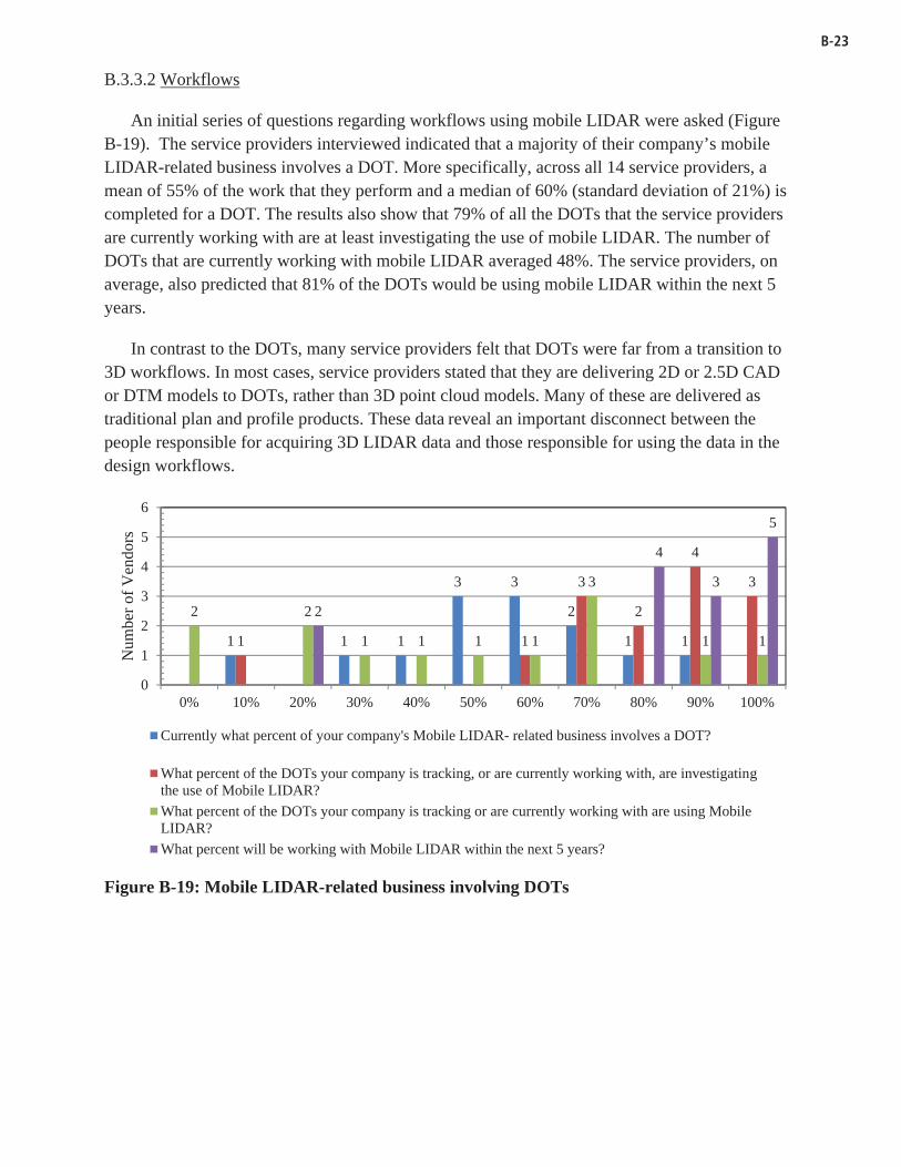
B-23

B.3.3.2 Workflows

An initial series of questions regarding workflows using mobile LIDAR were asked (Figure B-19). The service providers interviewed indicated that a majority of their company’s mobile LIDAR-related business involves a DOT. More specifically, across all 14 service providers, a mean of 55% of the work that they perform and a median of 60% (standard deviation of 21%) is completed for a DOT. The results also show that 79% of all the DOTs that the service providers are currently working with are at least investigating the use of mobile LIDAR. The number of DOTs that are currently working with mobile LIDAR averaged 48%. The service providers, on average, also predicted that 81% of the DOTs would be using mobile LIDAR within the next 5 years.

In contrast to the DOTs, many service providers felt that DOTs were far from a transition to 3D workflows. In most cases, service providers stated that they are delivering 2D or 2.5D CAD or DTM models to DOTs, rather than 3D point cloud models. Many of these are delivered as traditional plan and profile products. These data reveal an important disconnect between the people responsible for acquiring 3D LIDAR data and those responsible for using the data in the design workflows.

Figure B-19: Mobile LIDAR-related business involving DOTs

1 1 1

3 3

2

1 11 1

3

2

4

3

2 2

1 1 1 1

3

1 1

2

4

3

5

0

1

2

3

4

5

6

0% 10% 20% 30% 40% 50% 60% 70% 80% 90% 100%

Num

ber

of V

endo

rs

Currently what percent of your company's Mobile LIDAR- related business involves a DOT?

What percent of the DOTs your company is tracking, or are currently working with, are investigatingthe use of Mobile LIDAR?

What percent of the DOTs your company is tracking or are currently working with are using MobileLIDAR?

What percent will be working with Mobile LIDAR within the next 5 years?

B-24

When questioned regarding the use of 3D data by DOTs, the service providers reported, on average, that 80% of the DOTs were only using 2D/2.5D CAD and GIS software, 18.5% were transitioning to 3D model-based workflows, and 27.5% had already transitioned. However, it should be noted that three respondents were “not sure”, and five respondents stated that none of the DOTs have transitioned to 3D model-based workflows.

The service providers were asked to identify the top three issues holding back the adoption of 3D model-based workflows within DOTs (Figure B-20). Technical expertise and organizational issues were selected as the top two issues with 79% and 71%, respectively. The third most common response to this question, with a percentage of 36, was a tie between software, and “other”, which included concerns with management and workforce adaptation.

Regarding implementation challenges of mobile LIDAR scanning by state DOTs, service provider and state DOT responders showed some consistencies. Service providers identified technical expertise (57%), value proposition (29%), lack of standards (29%), and the size and complexity of datasets (29%) (Figure B-21). “Other” challenges included reluctance to accept the new technology, concerns with replacing tried and tested mapping methodologies and training, and a rigid procurement policy. Additionally, value proposition and inertia were each identified by 29% of service provider responders.

Figure B-20: Top three issues reported by service providers as holding back the adoption of 3D workflows in DOTs

79

2936

2921

71

36

0

20

40

60

80

100

Perc

enta

ge o

f V

endo

rs (

%)

What are the top 3 issues holding back the adoption of 3D model-based workflows in the DOTs?

B-25

Figure B-21: Top three factors delaying the adoption of mobile LIDAR by the DOTs

Regarding integration of mobile LIDAR with airborne or static GPS data, the service providers agreed that the process is generally straightforward, provided appropriate geo-referencing had been completed. One service provider mentioned that there can be some challenges with integration when combining lower accuracy data (e.g. inventory) with high accuracy data (e.g. engineering survey). In such cases, they felt that the dataset should be provided with a disclaimer. Several service providers mentioned that they have little experience with integrating airborne LIDAR data with mobile LIDAR data, but have integrated a substantial amount of static data with mobile to provide additional detail in areas where they could not get mobile LIDAR access. One respondent mentioned that most highway projects require the integration of multiple types of survey equipment (e.g., LIDAR, total station, etc.) to complete the necessary survey work for a project. Another respondent felt that in the future, the professional mapping firm would determine the appropriate tool for obtaining the best data rather than the DOT specifying the actual tool to collect the data.

The service providers were also asked how they perceived data was shared and managed within DOTs. The service providers responded that 69% of the DOTs manage data separately within each individual department and 31% of the DOTs manage data centrally and updated by each department.

57

29 29

14 14 14

21 21

14

29

7

36

0

20

40

60

Perc

enta

geof

Vend

ors

(%)

What are the top 3 factors delaying the adoption of Mobile LiDAR by the DOTs?

B-26

B.3.3.3 Applications (present and emerging)

Although the responding service providers currently support many of the applications they were asked about, service providers indicated that they anticipate supporting significantly more applications within the next five years, as shown in Figure B-22. Currently, most mobile LIDAR projects involve: engineering surveys, mapping, and DTM, with 100% of the service providers providing each of those applications. Applications that the service providers have been least involved with include: accident investigation (14%), slope stability/landslides analysis (43%), urban modeling/GIS (50%), and emergency response (50%).

Figure B-22: Supported applications by service providers currently and in the future

B.3.3.4 Challenges and need for guidelines

The service provider companies were asked to identify those areas where the proposed guidelines would assist their company in the procurement of mobile LIDAR/laser scanning

100 100 100

9386 86

93 93 93

86

79

93

50

71

79

93

21

93 93

79

57

71

86

71

79

50

64

79

14

43

50

64

50

0

20

40

60

80

100

Perc

enta

ge o

f V

endo

rs (

%)

Over the next 5 years which of the following Mobile LiDAR applications would yourcompany expect to support?

For the Mobile LiDAR projects that your company has been involved in what applicationshave the data been acquired for?

B-27

products and/or services. QA/QC procedures (86%), survey accuracy (64%), and data interoperability (57%) are the areas that were most often identified (Figure B-23). It was also mentioned that the purpose for acquiring the data, a checklist of possible data uses, lineage and traceability, and asset metadata were also important areas for guidance.

Figure B-23: Areas in which guidelines would be most helpful regarding the procurement of mobile LIDAR/laser scanning products and/or services

The service providers were asked about their familiarity with DOT published specifications.

Eleven of the 14 service providers responded that most DOTs have published surveying or quality control procedures. However, when asked whether most state DOTs that have surveying standards covering static laser scanning, only three service providers responded affirmatively. Similarly, service providers confirmed that most DOTs do not have mobile LIDAR standards. State DOTs identified with static LIDAR/laser scanning specifications include California, North Carolina, Michigan, Washington, and Texas. Caltrans and MoDOT were the only two DOTs identified as having specifications in place for mobile LIDAR. However, it was also mentioned that TexDOT was currently developing specifications. Michigan and New York were also identified as possibly having specifications, but the respondent was not sure.

Regarding the development of national standards, two service provider respondents felt that each DOT should develop their own static or mobile LIDAR standards, whereas 11 service provider respondents felt that a single standard should be adopted by all DOTs. One service provider did not respond. Comments from service provider respondents to this question included the following:

64

86

57

43 43

29

0

20

40

60

80

100

Perc

enta

ge o

f V

endo

rs (

%)

In what areas would DOT guidelines be most helpful to your company regarding the procurement of Mobile LiDAR/laser scanning products and/or

services?

B-28

Best practices or guidelines would be preferred over rigid standards. Standards may stifle innovation and can be confining. Flexibility is needed for projects and technology.

Standards could be like licensure requirements, in which there is a national standard with state supplements. New standards should be integrated into existing DOT standards.

Existing photogrammetry and survey standards could be adopted. Standards should focus on deliverables, not methodology.

Levels of detail include engineering survey, mapping, and asset grades.

When asked if performance-based specifications would be appropriate to use for mobile LIDAR, six respondents agreed they would be helpful. However, some of those provided the condition that “adequate QA/QC provisions are in place” and there is an “atmosphere of trust” between the agencies. The remaining respondents were not sure or did not respond to this question.

When asked what DOTs could do to streamline the adoption of mobile LIDAR, the responses from service providers included the following:

Exchange knowledge between DOTs.

Build from experience with airborne photogrammetry. Hire an expert consultant. Focus on deliverables/ end products rather than data acquisition. Develop standards or adopt guidelines. Use the recently developed Caltrans

specifications.

Adopt standards and develop good quality, clear Requests for Qualifications (RFQs), to avoid being disappointed with the results.

Be willing to experiment. Understand how mobile LIDAR can be used for multiple projects rather than narrowly

defining it by project. Learn how the data may be used by multiple divisions within an organization.

The determination of cost recovery in contracts must allow for new technology. Calculate cost savings from mobile LIDAR.

Realize the safety benefits of mobile LIDAR. Realize the changes in workflow from field to office.

Similarly, the service providers were asked what DOTs can do to streamline the procurement process for mobile LIDAR, which has been a challenge for many DOTs. Responses included:

Exchange knowledge between DOTs. Have a clear scope of the work, consistent with standards.

Focus on deliverables, not data collection.

B-29

Understand that most of the work for scanning is done in the office, not in the field.

Use qualification-based criteria (e.g., pilot projects for demonstration) rather than lowest bid. Implement more prequalified Indefinite Delivery Indefinite Quantity (IDIQ) projects.

Relax procurement guidelines that are locked into old procedures. Establish new rates for mobile LIDAR services. Allow requests for proposals (RFPs) to be accepted between states across state lines.

B.3.3.5 Accuracy and resolution requirements

Service providers were asked to provide the level of accuracy that their company would specify as being required for specific applications, such as engineering survey and pavement management (Table B-6). Some of the greatest accuracy discrepancies were reported for asset inventory and sign inventory, with a range of 90 to 56 cm respectively. Table B-7 shows the best horizontal and vertical accuracy (in cm) that the service providers specified as achievable with mobile LIDAR. The results from the responding service providers were transcribed into ranges, from the smallest accuracy required to the largest. The service providers provided responses in both SI and US customary units; however, all values were converted to SI units for ease of comparison.

Table B-6: Range of accuracies that the service providers specify as being required

Application MaximumError (cm)

MinimumError (cm) Range (cm)

Engineering survey 1 5 4 Bridge clearance 1 9 8

Paving 1 5 4 Drainage 1 6 5

Utility 1 30 29 Pavement 1 30 29

Sign inventory 5 61 56 Highway construction 2 5 3 Bridge construction 1 5 4

Asset inventory 10 100 90

B-30

Table B-7: Horizontal and Vertical accuracies stated as achievable by service providers

What is the maximum level of horizontal and ver cal accuracy that your company

specifies is achievable with mobile LIDAR?

Horizontal Ver cal

3 cm 1 to 1.5 cm

1.5 cm 1.5 cm

1.5 cm 0.9 cm

5 cm 5 cm

2.54 cm 2.54 cm

1.2 cm 1.8 cm

2 cm 3 cm

0.6 cm 0.6 cm

2 cm 2 cm

N/A 0.6 cm to 1.5 cm

5 cm 5 cm

The service providers were also asked what order of survey control was needed to achieve the desired accuracy. Three service providers said that the control varied and was condition-dependent, whereas one service provider said that no control was needed. Two service providers mentioned that under good GPS conditions, ground control points should be every 200 m (approximately 660 ft). One of these service providers also indicated that under poor GPS conditions, control points should be set every 100 m. A few service providers discussed the quality rating of the survey control used. One service provider stated that he/she only used first-order control; another stated that second-order control was acceptable; and a third stated that “high” order control was needed. Two service providers said that the recent Caltrans (2011) mobile LIDAR specifications govern the survey control they use.

B.3.3.6 Deliverables, and reporting

Most service providers agreed that the type of deliverable varies depending on the needs of the particular project and DOT. Potential deliverables identified by the service providers included the following:

1. Point clouds (raw, geo-referenced, or classified LAS file) 2. Viewing software 3. Calibrated imagery 4. Reports (methods, procedures, data quality achieved, control fit) 5. CAD or geodatabase files of extracted features 6. Planimetrics

B-31

7. DTM 8. Control surveys 9. Lineage documents 10. Corrected trajectory files 11. Check points 12. Ortho-photographs 13. Metadata

Some service providers expressed the belief that DOTs own the data from the mobile LIDAR services they pay for; however, some were concerned that the DOTs would be unable to use the full datasets. It was also mentioned that data ownership should be determined as part of the contract.

In addition to accuracy certification, many service providers agreed that reporting on the survey methodology was an important part of the project deliverables. Many mentioned that this information was critical to ensure that the results could be reproduced. However, three of the 14 service providers indicated that they should only be required to certify the final accuracy. These service providers felt that reporting the methodology would reveal proprietary information in some cases.

B.4 CONCLUSIONS

The DOT and service provider questionnaires provided valuable insights into the current and future plans of DOTs for the use of mobile LIDAR. These questionnaires established a technology adoption baseline that can be used to measure future progress. The DOT Questionnaire included responses from all 50 state DOTs in the U.S., plus a few other transportation agencies. The Service Provider Questionnaire included results from 14 highly experienced mobile LIDAR service providers.

Many personnel within the DOTs appear to be very interested in the use of scanning technology and feel that it will become a critical part of their operations in the next 5 years. The DOTs identified several applications for which they currently use mobile LIDAR and stated that they foresee expanding the use of the technology into numerous transportation applications over the next 5 years. The level of expertise related to mobile LIDAR among the DOTs showed substantial variability, particularly as compared to static scanning. Interestingly, more DOTs have used mobile than airborne LIDAR within the last year, even though mobile LIDAR technologies are comparatively less established.

Responders cited many challenges, both organizational and technical, that must be addressed before the DOTs can optimize the use of mobile LIDAR and completely integrate it into their workflows. One of the most significant challenges identified regarding the adoption of mobile LIDAR by DOTs was cost. This finding indicates that the respondents are not clear where

B-32

savings come from and what the return on investment is from mobile LIDAR. Additional education and evidence may be required to overcome this hurdle.

Comparison of the DOT and Service Provider Questionnaire results highlighted key differences between the perceptions of DOTs and service providers on the utility of 3D data. Most significantly, many service providers felt that DOTs were far from a transition to 3D workflows. However, most DOTs stated that they had transitioned or were well into the process of transitioning. These data reveal an important disconnect between the people responsible for acquiring LIDAR data and those responsible for the design workflows. Further, there are discrepancies between respondents as to what 3D is. As mobile LIDAR usage expands, it becomes increasingly important for both DOTs and service providers to understand how 3D data can be integrated into DOT workflows. All responders agreed that there are many challenges to overcome for a complete transition to 3D within DOTs.

The insights provided by this questionnaire form a framework to understand the key issues currently faced. Most DOTs believe very strongly that survey accuracy, QA/QC procedures, data interoperability, data management, and software integration are the most important topics to be addressed in the proposed guidelines, with nearly equal emphasis on each topic. Somewhat in contrast, the service providers believe that QA/QC procedures alone were by far the most important issue to address with the guidelines.

These insights were incorporated in the development of these national guidelines, which will assist transportation personnel in utilizing mobile LIDAR effectively for a variety of applications.

B-33

B.5 DOT QUESTIONNAIRE

GUIDELINES FOR THE USE OF MOBILE LIDAR IN TRANSPORTATION APPLICATIONS

Dear survey participant, Your organization has been identified as an important contributor to this project. As part of NHCRP15-44 "Guidelines for the Use of Mobile LIDAR in Transportation Applications" the research team needs to acquire information related to the following objectives: 1. Determining the current and planned use of mobile LIDAR to support survey, project planning, project development, construction, operations, maintenance, safety, research and asset management. 2. Understanding the implications associated with the use of mobile LIDAR on design, construction, contracting practices, data management, and other related issues within your organization. Your organization's expertise and experience is critical to the success of this important project. The survey is organized into two parts based on the objectives listed above. The survey should take approximately 15 minutes to complete. Once again we thank your organization in advance for your time and thoughtful consideration. Please pass this survey onto others who could add value to this effort. Should you have any questions or concerns, or if you would like more information regarding this project, please contact: Michael Olsen, Ph.D. Assistant Professor of Geomatics School of Civil and Construction Engineering Oregon State University Email: michael.olsen@oregonstate.edu Phone: (541)-737-9327 http://apps.trb.org/cmsfeed/TRBNetProjectDisplay.asp?ProjectID=2972

B-34

1) Please provide the name of your organization/DOT ____________________________________________ 2) Within your unit of your organization, what types of services does your unit provide? Multiple selections ok [ ] Asset Management/Inventory [ ] Construction [ ] Engineering Design [ ] Geomatics/Surveying [ ] Maintenance [ ] Operations [ ] Project Planning [ ] Project Development [ ] Research [ ] Safety [ ] Other

3) How familiar are members of your department with 3D laser scanning and/or LIDAR? Unfamiliar Expert ( ) Not Sure ( ) 1 ( ) 2 ( ) 3 ( ) 4 ( ) 5 ( ) 6 ( ) 7 ( ) 8 ( ) 9 ( ) 10 4) How familiar are members of your department with mobile LIDAR/laser scanning systems? Unfamiliar Expert ( ) Not Sure ( ) 1 ( ) 2 ( ) 3 ( ) 4 ( ) 5 ( ) 6 ( ) 7 ( ) 8 ( ) 9 ( ) 10 5) How important are these technologies to the future operations within your organization? Not Important Very Important ( ) Not Sure ( ) 1 ( ) 2 ( ) 3 ( ) 4 ( ) 5 ( ) 6 ( ) 7 ( ) 8 ( ) 9 ( ) 10 6) Additional comments?

7) Does your organization currently have published surveying and/or quality control standards? ( ) Yes ( ) No How familiar are members of your department with the current field surveying and related quality control standards within your organization? Unfamiliar Expert ( ) Not Sure ( ) 1 ( ) 2 ( ) 3 ( ) 4 ( ) 5 ( ) 6 ( ) 7 ( ) 8 ( ) 9 ( ) 10 Do your organization's current published surveying standards cover the use of static laser scanning? ( ) Yes ( ) No Do your organization's current published survey standards cover the use of mobile LIDAR/laser scanning? ( ) Yes ( ) No 8) Additional comments?

9) Currently what percent of surveying work/data acquisition is performed in-house vs. contracted out to private firms? ( ) 0% ( )10% ( )20% ( )30% ( )40% ( )50% ( )60% ( )70% ( )80% ( )90% ( )100% ( )Not Sure

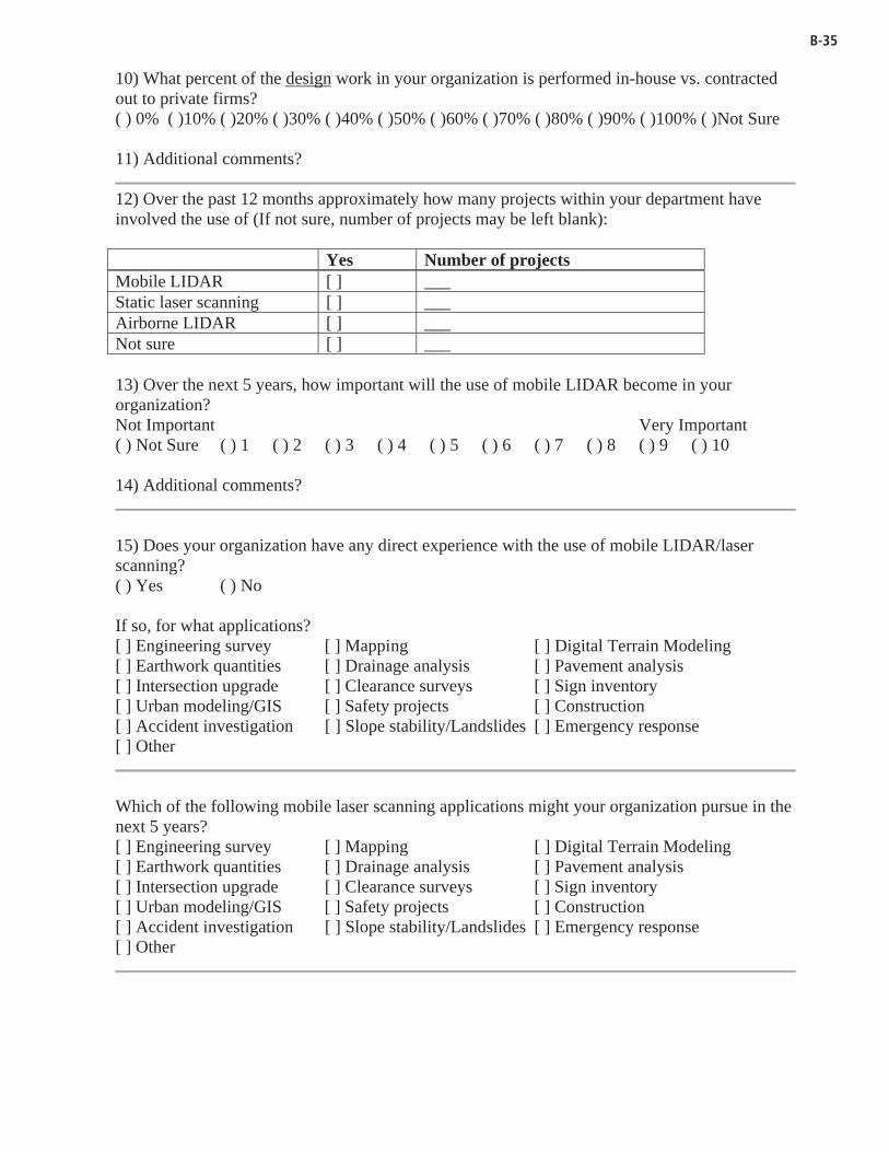
B-35

10) What percent of the design work in your organization is performed in-house vs. contracted out to private firms? ( ) 0% ( )10% ( )20% ( )30% ( )40% ( )50% ( )60% ( )70% ( )80% ( )90% ( )100% ( )Not Sure 11) Additional comments?

12) Over the past 12 months approximately how many projects within your department have involved the use of (If not sure, number of projects may be left blank):

Yes Number of projects Mobile LIDAR [ ] ___ Static laser scanning [ ] ___ Airborne LIDAR [ ] ___ Not sure [ ] ___ 13) Over the next 5 years, how important will the use of mobile LIDAR become in your organization? Not Important Very Important ( ) Not Sure ( ) 1 ( ) 2 ( ) 3 ( ) 4 ( ) 5 ( ) 6 ( ) 7 ( ) 8 ( ) 9 ( ) 10 14) Additional comments?

15) Does your organization have any direct experience with the use of mobile LIDAR/laser scanning? ( ) Yes ( ) No If so, for what applications? [ ] Engineering survey [ ] Mapping [ ] Digital Terrain Modeling [ ] Earthwork quantities [ ] Drainage analysis [ ] Pavement analysis [ ] Intersection upgrade [ ] Clearance surveys [ ] Sign inventory [ ] Urban modeling/GIS [ ] Safety projects [ ] Construction [ ] Accident investigation [ ] Slope stability/Landslides [ ] Emergency response [ ] Other

Which of the following mobile laser scanning applications might your organization pursue in the next 5 years? [ ] Engineering survey [ ] Mapping [ ] Digital Terrain Modeling [ ] Earthwork quantities [ ] Drainage analysis [ ] Pavement analysis [ ] Intersection upgrade [ ] Clearance surveys [ ] Sign inventory [ ] Urban modeling/GIS [ ] Safety projects [ ] Construction [ ] Accident investigation [ ] Slope stability/Landslides [ ] Emergency response [ ] Other

B-36

16) What challenges has your organization experienced when performing mobile LIDAR surveys [ ] Accuracy [ ] Cost [ ] Availability [ ] Weather related [ ] Technical expertise [ ] Traffic [ ] Size and complexity of datasets [ ] Software interoperability/data exchange [ ] Organizational [ ] No challenges [ ] Don't perform mobile scans [ ] Other challenges

17) In what areas would guidelines be most helpful to your organization regarding the use of mobile LIDAR/laser scanning? [ ] Survey accuracy [ ] QA/QC procedures [ ] Data interoperability [ ] Data management [ ] Software integration [ ] Other 18) Additional comments?

19) Where is your organization in terms of the transition from 2D to 3D? ( ) We use only 2D CAD and GIS software ( ) We are currently transitioning to 3D workflows ( ) We have transitioned to 3D workflows in software such as CAD and GIS ( ) Not sure 20) Additional comments?

21) Currently, what percent of the technical workflows in your organization use 3D data? ( ) 0% ( )10% ( )20% ( )30% ( )40% ( )50% ( )60% ( )70% ( )80% ( )90% ( )100% ( )Not Sure 22) What percent of the overall technical workflows in your organization would benefit from the use of 3D data and/or visualization? ( ) 0% ( )10% ( )20% ( )30% ( )40% ( )50% ( )60% ( )70% ( )80% ( )90% ( )100% ( )Not Sure 23) What is holding back the adoption of 3D workflows? [ ] Technical expertise [ ] Value proposition [ ] Software [ ] Inertia [ ] Funding [ ] Organizational issues [ ] Not Sure [ ] Other 24) Additional comments?

25) What is the level of accuracy and resolution required to support each of your departments's daily workflows?

Accuracy Resolution mm level [ ] [ ] cm level [ ] [ ] dm level [ ] [ ] m level [ ] [ ]

B-37

26) How is geospatial/survey data currently managed within your organization? ( ) Centrally located and updated by each department ( ) Differently within each individual department 27) Additional comments?

28) Can you recommend other individuals in your organization that would have an interest in responding to this survey? 29) Who is the primary contact for geospatial technology in your organization, and what is that individual's contact information?

Thank You! Thank you for participating in our survey. Your response is very important to us. If you are interested in the results of the project please contact: Dr. Michael Olsen Assistant Professor of Geomatics School of Civil and Construction Engineering Oregon State University Email: michael.olsen@oregonstate.edu Phone: (541)-737-9327

B-38

B.6 SERVICE PROVIDER QUESTIONNAIRE

GUIDELINES FOR THE USE OF MOBILE LIDAR IN TRANSPORTATION APPLICATIONS

Hello. Your company has been identified as a potential contributor to an important Transportation Research Board –TRB project. As part of NCHRP 15-44, entitled “Guidelines for the Use of mobile LIDAR in Transportation Applications" the research team is in the process of acquiring information from all of the DOTs, transportation related agencies, and the service provider community here in the US. The primary objectives of these surveys and interviews are to: 1. Determine the current and planned use of mobile LIDAR within the DOTs in support of survey, project planning, project development, construction, operations, maintenance, safety, research and asset management. 2. Understand the implications associated with the use of mobile LIDAR by the DOTs for design, construction, contracting practices, data management, and other related activities. In addition to the DOTs the research team is also interviewing a limited number of service providers that are involved with the use of mobile LIDAR. We are seeking input from the service provider community concerning how the DOTs can make the transition to the use of mobile LIDAR data acquisition as streamlined as possible. Your organization's expertise and experience is critical to the success of this important project. The interview is organized into two parts based on the objectives listed above. The interview should take approximately 30 minutes to complete. Should you have any questions or concerns, or if you would like more information regarding this project, please contact: Michael Olsen, Ph.D. Assistant Professor of Geomatics School of Civil and Construction Engineering Oregon State University http://apps.trb.org/cmsfeed/TRBNetProjectDisplay.asp?ProjectID=2972 PLEASE NOTE: At the top of every page there is a link that allows you to save your work and continue the survey at a later time.

B-39

1) Company Name ____________________________________________ 2) Department Name (if applicable) ____________________________________________

3) How long has your company been involved with 3D laser scanning and/or static LIDAR? ( ) Not Sure ( ) Years: _________________ 4) How long has your company been involved with mobile LIDAR/laser scanning systems? ( ) Not Sure ( ) Years: _________________

5) On a scale of 1 to 10, where 10 is extremely important, how important are LIDAR-based acquisition technologies to future DOT survey operations? Not Important Very Important ( ) Not Sure ( ) 1 ( ) 2 ( ) 3 ( ) 4 ( ) 5 ( ) 6 ( ) 7 ( ) 8 ( ) 9 ( ) 10

6) Do most DOTs currently have published surveying and/or quality control standards? ( ) Yes ( ) No Please Identify DOTs with Standards

7) Do most DOTs current published surveying standards cover the use of static laser scanning? ( ) Yes ( ) No Please Identify DOTs with Standards

8) Do most DOTs current published survey standards cover the use of mobile LIDAR/laser scanning? ( ) Yes ( ) No Please Identify DOTs with Standards

9) Does your company recommend that each DOT develop their own static laser scanning and/or mobile LIDAR standards? ( ) Yes ( ) No 10) If not, would a single standard that all DOTs adopt be preferred? ( ) Yes ( ) No 11) Additional Comments?

12) Currently what percent of your company's mobile LIDAR- related business involves a DOT? ( ) 0% ( )10% ( )20% ( )30% ( )40% ( )50% ( )60% ( )70% ( )80% ( )90% ( )100% ( )Not Sure 13) What percent of the DOTs your company is tracking, or are currently working with, are investigating the use of mobile LIDAR? ( ) 0% ( )10% ( )20% ( )30% ( )40% ( )50% ( )60% ( )70% ( )80% ( )90% ( )100% ( )Not Sure

B-40

14) What percent of the DOTs your company is tracking or are currently working with are using mobile LIDAR? ( ) 0% ( )10% ( )20% ( )30% ( )40% ( )50% ( )60% ( )70% ( )80% ( )90% ( )100% ( )Not Sure 15) What percent will be working with mobile LIDAR within the next 5 years? ( ) 0% ( )10% ( )20% ( )30% ( )40% ( )50% ( )60% ( )70% ( )80% ( )90% ( )100% ( )Not Sure

16) For the mobile LIDAR projects that your company has been involved in what applications have the data been acquired for? Choose all that apply [ ] Engineering survey [ ] Mapping [ ] Digital Terrain Modeling [ ] Earthwork quantities [ ] Drainage analysis [ ] Pavement analysis [ ] Intersection upgrade [ ] Clearance surveys [ ] Sign inventory [ ] Urban modeling/GIS [ ] Safety projects [ ] Construction [ ] Accident investigation [ ] Slope stability/Landslides [ ] Emergency response [ ] Other

17) Over the next 5 years which of the following mobile LIDAR applications would your company expect to support? Choose all that apply [ ] Engineering survey [ ] Mapping [ ] Digital Terrain Modeling [ ] Earthwork quantities [ ] Drainage analysis [ ] Pavement analysis [ ] Intersection upgrade [ ] Clearance surveys [ ] Sign inventory [ ] Urban modeling/GIS [ ] Safety projects [ ] Construction [ ] Accident investigation [ ] Slope stability/Landslides [ ] Emergency response [ ] Other

18) In what areas would DOT guidelines be most helpful to your company regarding the procurement of mobile LIDAR/laser scanning products and/or services? Check all that apply. [ ] Survey accuracy [ ] QA/QC procedures [ ] Data interoperability [ ] Data management [ ] Software integration [ ] Other

19) What percent of DOTs that your company works with are: Percentages must add to 100%

% Only using 2D/2.5D CAD and GIS software ___ Currently transitioning from 2D/2.5D to 3D model-based workflows ___ Have transitioned from 2D/2.5D to 3D model-based workflows in software such as CAD and GIS

___

( ) Not sure

B-41

20) What are the top 3 issues holding back the adoption of 3D model-based workflows in the DOTs? [ ] Technical expertise [ ] Value proposition [ ] Software [ ] Inertia [ ] Funding [ ] Organizational issues [ ] Not Sure [ ] Other 21) What are the top 3 factors delaying the adoption of mobile LIDAR by the DOTs? [ ] Technical expertise [ ] Value proposition [ ] Lack of standards [ ] Misinformation [ ] Software [ ] Inertia [ ] Funding [ ] Organizational issues [ ] Requirement for 2D deliverables [ ] Size and complexity of datasets [ ] Software interoperability/data exchange [ ] No challenges [ ] Cost [ ] Other challenges 22) What could the DOTs do to streamline the adoption of mobile LIDAR? 23) What can the DOTs do to streamline the procurement process for mobile LIDAR?

24) What is the maximum level of horizontal and vertical accuracy that your company specifies is achievable with mobile LIDAR? 25) What order of survey control is needed to achieve this? Please specify methods used. 26) What level of accuracy and minimum point density would your company specify as being required for each of the following:

Accuracy Minimum Point Density Engineering survey ___ ___ Bridge Clearance ___ ___ Paving ___ ___ Drainage ___ ___ Utility ___ ___ Pavement management ___ ___ Sign inventory ___ ___ Highway construction ___ ___ Bridge construction ___ ___ Asset inventory ___ ___ 27) Is it necessary for a mobile LIDAR service provider to report on their survey methodology as part of the project deliverable, or just certify as to the final accuracy? Please explain. 28) What does your company think should be included as part of the final deliverables from a mobile LIDAR survey? 29) How do you see the use of mobile LIDAR fitting in with the increasing use of performance-based specifications? 30) How is your company integrating airborne/static and mobile LIDAR data?

B-42

31) How does your company perceive that geospatial/survey data is currently managed within the DOTs in general? ( ) Centrally located and updated by each department ( ) Differently within each individual department

32) Can you recommend other individuals that might have an interest in responding to this survey? 33) Is there a primary contact for mobile LIDAR in your organization, and what is that individual's contact information? 34) Any additional comments or concerns?

Thank You! Thank you for participating in our survey. Your response is very important to us. If you are interested in the results of the project please contact: Dr. Michael Olsen Assistant Professor of Geomatics School of Civil and Construction Engineering Oregon State University Email: michael.olsen@oregonstate.edu Phone: (541)-737-9327

C-1

A p p e n d i x C

Statement of Work (Outline)

PROJECT TITLE Contacts

List contact information for primary representative of data\service provider, transportation agency, and any other organization involved.

Background

The background will include the purpose and expected outcomes of the project. This will serve as communication to ensure the service provider understands the intent of the transportation agency for data acquisition and the transportation agency understands what is feasible.

The intended application(s) and user(s) of the data should be discussed.

Project Location

Insert graphic or link to project limits and annotations for areas of special consideration. Note the sections of interest, and estimated length of project (including interchanges, ramps, etc.).

Type of highway to be surveyed (interstate, urban highway, rural highway, etc.).

Agency Standard References

List references (such as this Guidelines document and FGDC 1998) that will be followed for completion of the work.

Professional Licensure Expectations

Does the work require a Professional Land Surveyor, Professional Engineer, and/or Certified Photogrammetrist?

C-2

Work Plan

Task 1 Project Management

Coordination (Meetings, Teleconferences, Milestone reviews)

Budget (Tracking, Reporting) Schedule (Tracking, Reporting) – should include field and office processing

timeframes

Quality Management Report Progress Reports Survey Narrative Report Calibration requirements

Task 2 Project Planning

Data Collection Plan (Survey Control, Collection Routes, GNSS Constellation Review, etc.)

Safety Plan (Emergency Contacts, Daily safety assessment, Traffic concerns, etc.)

Task 3 Horizontal/Vertical Control

Coordinate System used including Horizontal and Vertical Datum and Units

Description of existing control expectations including monumentation, reference networks, GPS baseline lengths, etc.

Survey Control Report

Task 4 Mobile Scanning Collection and Processing

Point cloud accuracy and resolution expectations (data collection category)

Point cloud deliverable format (including whether RGB and Intensity values are needed)

Imagery requirements Processing techniques

Resources To Be Provided By Transportation Agency

What the data provider can expect from the transportation agency such as road access (e.g., rolling slow down, control points, etc.).

Approach

Details on equipment to be used and expertise of service provider.

C-3

Software formats

Viewing software, if needed

Project Schedule/Timeline

Graphic showing when each task will occur, including start and completion dates Delivery Schedule

When and where products should be delivered

Acceptance Criteria

Discussion on what must be met for payment and if a pay scale will be used. Who will perform the QA/QC work (data provider, transportation agency, or external)? Accuracy should be reported following the FGDC standards.

Compensation

Discussion of costs involved with the project and how payments will be made

Appendix:

Acronyms and definitions

Task 5 Mapping/Modeling

Data formats required for deliverables Extracted Points with attributes (classification)

Digital Terrain Model

2D or 3D linework/shapefiles 3D solid model

D-1

A p p e n d i x d

Sample Calibration Report

CALIBRATION REPORT

System#: ___________________

Signed Out Date:

Signed Off By:

First Project Name/Number Project Manager:

Signed In Date:

CALIBRATION CERTIFICATION I certify that the testing and calibration of this system has been performed in accordance with customary procedures and that this system meets required performance specifications unless noted otherwise. Authorized Calibration Engineer Date

D-2

MLS SYSTEM CONFIGURATION REPORT BY: ____________________ Date[yyyy/mm/dd]: ____ /___ /____

COMPUTER RACK DESCRIPTION:

Logging CPU Number ______________ Nav CPU Number ____________

S/N P/N

______________________________________________________________ ____ _

S/N P/N

__________________________________________________________________

Disk (GB) ______________ Disk (GB) ____________

Monitor S/N __________________ P/N __________________

Keyboard S/N P/N

____________________________________________________

GPS Model ________________________ GPS Firmware: ___________

GPS S/N ________________________ Antenna S/N: _____________

DMI Model ________________________ Install Location:___________

DMI S/N ________________________

INSTRUMENT PLATE DESCRIPTION:

Type of Plate Plate Number

Laser #1 Model Unit #: _____ S/N ______________________________

Laser #2 Model Unit #: _____ S/N ______________________________

IMU Model Unit #: _____ S/N ______________________________

Camera #1 Model Unit #: _____ S/N _____________ Lens#:________

Camera #2 Model Unit #: _____ S/N ______________ Lens#:________

Pod Type:

D-3

Installation Diagram

Installation Notes

D-4

IMU to Laser #1 Boresights

Boresight Component Angle (degrees)

Estimated Accuracy (1 , meters) Date Computation Method

Roll

Pitch

Yaw

IMU to Laser #1 Offsets (IMU-Laser)

Offset Component Value (meters)

Estimated Accuracy (1 , meters) Date Computation Method

X

Y

Z

IMU to Laser #2 Boresights

Boresight Component Angle (degrees)

Estimated Accuracy (1 , meters)) Date Computation Method

Roll

Pitch

Yaw

IMU to Laser #2 Offsets (IMU-Laser)

Offset Component Value (meters)

Estimated Accuracy (1 , meters) Date Computation Method

X

Y

Z

D-5

IMU to Camera #1 Boresights

Boresight Component Angle (degrees)

Estimated Accuracy (1 , meters) Date Computation Method

Roll

Pitch

Yaw

IMU to Camera #1 Offsets (IMU-Camera)

Offset Component Value (meters)

Estimated Accuracy (1 , meters) Date Computation Method

X

Y

Z

IMU to Camera #2 Boresights

Boresight Component Angle (degrees)

Estimated Accuracy (1 ) (meters) Date Computation Method

Roll

Pitch

Yaw

IMU to Camera #2 Offsets (IMU-Camera)

Offset Component Value (meters)

Estimated Accuracy (1 ) (meters) Date Computation Method

X

Y

Z

D-6

IMU to GPS Offsets (IMU-GPS)

Offset Component Value (meters)

Estimated Accuracy (1 ) (meters) Date Computation Method

X

Y

Z

IMU to DMI Offsets (IMU-DMI)

Offset Component Value (meters)

Estimated Accuracy (1 ) (meters) Date Computation Method

X

Y

Z

E-1

A p p e n d i x e

Current Storage Formats

Information processed into point clouds or similar structures can be represented and stored using numerous formats. This appendix elaborates on the most common formats used in MLS applications. Formats used for video, imagery, models or other information are not discussed.

E.1 COMMON FORMATS

The common formats available today and their characteristics are listed below, along with a brief description. The LAS format is the most widely used for MLS systems, is integrated into most software packages, and has the longest history. For these reasons it is recommended for use by transportation agencies at this time. The ASTM E57 format, however, does provide unique features such as integrated, calibrated imagery, which may be of interest to a transportation agency once the format is adopted by vendors of kinematic laser scanning software. Ultimately, a transportation agency should evaluate which format will integrate best with their workflows. The ASCII format is described here for completeness, but is not recommended because it is not clearly defined, and has other limitations described below.

E.1.1 ASCII

Despite common usage, this term does not refer to a file format per se. Point clouds represented in ASCII consist typically of coordinate information written in decimal format, with spaces and other formatting characters inserted to improve human readability. Usually, each line in an ASCII file represents a single point. Optionally, ASCII “formats” may also include additional information about each point, such as color, strength of the return signal, or surface direction. Decimal notation is deceptively flexible, in part because the notion of resolution is built-in: most will recognize the distinction between, say, 3.14 and 3.141592 used to represent a coordinate. If the measurement is taken as meters, the first number implies an uncertainty of ±1 centimeter, whereas the latter implies an uncertainty of ±1 micrometer. One downside to this simplicity is that to increase resolution by one decimal place (a factor of 10) requires writing an additional digit, at a storage cost significantly greater than necessary. Another downside is that it is too easy for software packages to inadvertently truncate ASCII data—perhaps using single-precision operations rather than double-precision floating point operations—and thereby reduce the accuracy and precision of the data.

E-2

The popularity of ASCII can be attributed to its simplicity, and the availability of standard tools for working with small data sets. However, when dealing with millions or billions of points, the drawbacks of ASCII are clear: first, decimal notation is not efficient. A number stored with 4 bytes in binary may require 10 or more bytes in ASCII. Second, converting from binary to decimal or vice versa is time-consuming (even by computer standards) and adds significant overhead to file reading or writing and processing. And third, the widespread availability of tools that may be used to modify the contents of an ASCII file may lead to data corruption and untraceable activity by inexperienced operators, particularly since such tools are not likely designed to handle such large amounts of data.

E.1.2 LASer (LAS) file format exchange

The ASPRS created the LAS format, in part, to address the shortcomings of using ASCII for working with LIDAR data. It is an open standard, meaning that the specification is publically available and that vendors are free to adopt the standard for reading and writing of files. LAS is a binary format that was originally developed for airborne LIDAR systems and upgraded at version 1.4 (November 2011) to address MLS as well. It can also be used for data collected by stationary LIDAR scanners although it does not support spherical or cylindrical coordinate systems. Typically, the bulk of an LAS file consists of point cloud information. Each point is represented by a 3D coordinate and intensity information, multiple return and source data, and optionally color, GPS time (i.e., globally referenced time at which the point was acquired), and waveform data. Depending on the amount of optional information desired, the LAS format typically requires between 20 and 34 bytes per point. However, if waveform data is included, additional bytes are required, but the actual number is variable depends on several hardware- and project-specific considerations.

An important feature of the LAS format is that each point may is identified with a particular type, or class, of object type. It supports up to 256 classes, assigned by integer values. ASPRS standard classes are shown in Table E-1.

LAS is a well-defined and popular format that is straightforward to work with at a software level. The binary foundation is an improvement to ASCII in both speed and size. The current format does not support compression for point data, though it is expected that future versions will support compression for waveform data (LAS 1.4 r12, 2011). The most up-to-date version of LAS is v1.4. This format also offers the ability to select additional information that is associated with the 3D points. Prior to LAS v1.4, the user was only allowed to select various pre-configured formats. However, LAS v1.4 now provides the ability to store an optional, extra byte, variable length record. MLS and software manufacturers will hopefully take advantage of this capability to preserve unique features of mobile scanners.

The notion of readability is also misleading. No computer file is actually human-readable: a collection of software programs, operating systems, and hardware converts the bits on disk into glyphs on screen or paper that are familiar. Therefore, “human-readable” should be understood as a format that is easily manipulated by simple and ubiquitous tools (such text editors) that are freely available on typical computer systems.

E-3

Table E-1: ASPRS Standard LIDAR Point Classes

Classifica�on Value Defini�on0 Created, never classified1 Unclassified2 Ground3 Low Vegeta�on4 Medium Vegeta�on5 High Vegeta�on6 Building7 Low Point (noise)8 Model Key point (mass point)9 Water10 Reserved for ASPRS Defini�on11 Reserved for ASPRS Defini�on12 Overlap Points13 31 Reserved for ASPRS Defini�on

One important consideration when working with LAS formats is the Point Record type that is used within the file. Each version of LAS supports a particular set of Point Records, each supporting particular attributes that are recorded along with coordinate data. It is beyond the scope of this document to describe the various Point Records in detail, other than to say that it is recommended to use Point Record 6 of above whenever practical.

E.1.3 LAZ

LAZ is a compressed version of the LAS format. It is completely lossless at the bit level: each bit within the original LAS file is recoverable when the LAZ file is decompressed. LAZ files are typically only 10-20 percent the size of the original LAS file. Created in conjunction with the LAZ format was the LASzip compression library. This library provides users and software developers with the tools to convert from LAS to LAZ and vice versa. The library is licensed using the GNU Lesser General Public License (LGPL), which requires the library and all modifications, extensions and derivative works to be freely available, subject to certain conditions. Importantly, the LGPL version of the GNU licensing schemes does not require applications that only link to the library to be free. This means that independent vendors can use the LASzip libraries within their proprietary software applications. Such applications are able to read and write LAZ files without creating any intermediate LAS files. The tradeoff for reduced file size is longer read/write times as well as any issues that may arise from any bugs or deficiencies in the implementation of the library. LAZ does not currently support LAS files with waveform data packets.

E.1.4 E57

Recently, the ASTM E57 committee developed specifications for 3D imaging systems, including terrestrial laser scan data. The ASTM E57 file format is designed to be flexible in storing data across a broad range of applications. Externally, it incorporates much of the same data as the LAS format, but internally the data is stored significantly differently. For example, the E57 format supports variable resolution by allowing a user to specify the number of bits to be

E-4

used to represent the captured data as well as the type of coordinate system (e.g., spherical, cylindrical, or Cartesian) used to store the data. The latter may reduce the number of bits required to store a point by more closely matching the data to the electronic or mechanical configuration of the scanning system. The maximum file size of E57 data is practically unlimited, adding additional flexibility to data management (Huber, 2011). However, users are cautioned against creating very large files that cannot efficiently be handled by operating systems and applications. This format is important for use with static scan data because it preserves internal scanning grid structures that are lost in other formats. While E57 currently does not fully support data from kinematic scanning (other than basic point and other information), this format is only in its first release and likely will evolve rapidly.

Furthermore, E57 provides extensive support for ancillary imagery, including enabling calibrated imagery to be stored along with the point cloud, which is not available in other formats. When 2D imagery is collected in conjunction with 3D LIDAR information, the raw information is typically stored in separate files in industry-standard formats (e.g., jpg). The E57 format supports the additional step of converting the raster 2D image into a calibrated image for which each pixel corresponds to a calibrated ray extending outward from the camera. Having this information available to software applications in a standard way should give rise to tighter integration between the LIDAR and image sensors and improve the quality of downstream processing and use.

The E57 format is designed to be easily extensible. Adding new data fields to a point cloud can be done in a standard way, but there are several fields of interest that are not currently supported by this format. In particular, the most recent specification does not natively support either the LAS classifications for points or scan line information. While it is relatively straightforward for 3rd party vendors to do so, such extensions are non-standard and therefore potentially problematic from a data or lifecycle management perspective.

This format has only recently been released and is in the process of being integrated into mainstream software packages for static scanning. Future versions are anticipated to fully support kinematic laser scanners including data acquisition structure and sensor stream information. Further, although E57 does not currently support meaningful compression, that is likely to change within the next few years.

E.2 PROPRIETARY FORMATS

Numerous vendors and other entities have developed formats for recording point cloud information. Most are binary (in order to handle large data sets) and are often closed formats. The advantage of proprietary formats is that they are optimized for a particular software package or application. (Hence, they are efficient working formats). However, the disadvantages are numerous, including:

Difficulty (and data loss) transferring between formats or applications;

Single source for support and maintenance;

E-5

Risk that the vendor ceases to support or modifies the format; and Locking into a specific vendor or package.

For these reasons, proprietary formats should be used sparingly (and with appropriate knowledge) in any work process and should be avoided for archival or data sharing.

E.3 COMPARISON

Table E-2 provides a comparison of the salient characteristics of several commonly used point cloud formats. In this table,

‘Organization and Specification link’ refer to the sponsoring or creating entity and an Internet location for more information about the specification;

‘Current version’ is as of August 2012; ‘Coordinate system support’ indicates if the format can natively handle supplying data in a variety of standard systems, such as UTM or state plane;

‘Focus’ gives the initial motivation for the development of the format; ‘Read/write speeds’ provide a rough comparison (no quantitative estimates are possible because actual speeds depend heavily on file size, point geometry, software application, network configuration, and hardware selection);

‘Software integration’ offers suggestions as to how widely used the format is;

‘Metadata & Classification’ can be stored either within the file or externally;

‘Classification supported’ may either be internal to the file; ‘Image support’ refers to how the format may handle geospatially calibrated color imagery;

‘File Size’ entries offer estimates for files consisting of points with color and intensity values stored;

‘Mobile LIDAR support’ includes a discussion of specific considerations for use of the format with mobile LIDAR.

‘Ability to customize’ may be important for some users, and it is important to note that any customization will likely require deep familiarity with the format and extensive software development skills. This attribute is more for software vendors than users.

‘Data not directly incorporated in file’ shows some of the types of data that have to be handled separately during collection and processing.

‘Integrated checksum’ indicates whether the file format has a built-in mechanism to maintain file integrity in the face of hardware or possibly software glitches. Most computer systems rely on the operating system to enforce file integrity. This ability has improved with file systems such as NTFS, which includes Error Detection and Correction (EDAC). However, with large data sets it is helpful to have checksums within the file so applications may verify the integrity continually during use and edit sessions.

E-6

Table E-2: Comparison of Common Point Cloud File Formats.

Format LAS LAZ* E57 ASCII Organization ASPRS Martin Isenberg ASTM - Specification link

http://www.asprs.org/a/society/committees/standards/LAS_1_4_r11.pdf

http://www.laszip.org/

http://www.libe57.org/

Not applicable

Current version (year)

1.4-R12 (2011) 2.1.0 (2012) V1.0 (2011) Not applicable

Coordinate System Support

Supports Cartesian coordinates and map projections.

Supports Cartesian coordinates and map projections.

Fully supports Cartesian, spherical, and cylindrical coordinate systems and map projections. Transformation matrices also can be integrated.

None

Focus Kinematic laser scanning working format

Kinematic laser scanning working or archive format

Archive/ interchange format for static TLS and 3D imaging devices.

Generic format adapted to suit need. Very limited on what can be stored.

Read/write speeds & considerations

Fast, require little processing to bring into computer memory.

Fast. Smaller files are quicker to move across network, but require time to compress/ decompress.

Relatively fast, but a compressed version is not available yet.

Slow, text must be parsed.

Software integration

Most packages support a version of LAS. Ver. 1.4 is currently being adopted.

Adoption in progress, some packages support.

Adoption in progress, some support, but increasing rapidly.

Packages support, but data may be lossy, bulky, and slow.

Metadata & Classification

Internal Internal Internal External or Additional fields, may not be supported in software packages.

E-7

Format LAS LAZ* E57 ASCII Image support

RGB colors mapped to points only. No Image support.

RGB colors mapped to points only. No Image support.

Full image support\links, including calibration.

RGB colors mapped to points only.

Mobile LIDAR support

Most commonly used format for mobile LIDAR.

Will likely be very common in near future.

A mobile LIDAR format is under development.

Lossy: Can store derivative data (Coordinates, RGB, Intensity).

Ability to customize

Limited Limited Flexible Flexible but limited and lossy.

Data not directly incorporated in file (general) Note that other data such as GNSS and IMU data can be stored in separate files and linked with a time stamp.

Inter-relationship structure between scan points GNSS IMU Images Image Calibration

Inter-relationship structure between scan points GNSS IMU Images Image Calibration

GNSS IMU

Scanner properties Inter-relationship between scan points Geo-referencing parameters GNSS IMU Images Image Calibration

Max File Size Practically unlimited, 264 records

Practically unlimited, 264 records

Nearly unlimited, (18 exabytes)

Difficult to work with after 1GB.

Integrated Checksum

No No Yes, at fine scale.

No

Other comments

Most mature format

Lossless compression from LAS

Preserves structure (rows, columns, or user-defined) of data collection (e.g. grid pattern for sTLS).

Slow, use only when no other options.

*LAZ is a compressed version of the LAS format and is not an independent format.

E-8

E.3.1 Evaluations

As discussed above, there are several formats for distribution and use of MLS data. While at this time the LAS format is recommended, the industry is evolving rapidly and therefore it is not possible to give hard-and-fast rules as to which formats may be preferable in the future. Each organization must make its own decisions according to the following criteria:

a. Compatibility with selected software applications b. Long-term stability of the format(s) c. Compression vs. speed tradeoffs

Clearly the chosen format should be compatible with the desired software applications. Most

applications are, on the surface, compatible with the major formats, but it is important to also consider the level of compatibility: Is a conversion to a proprietary format necessary? If so, does the application require a lengthy batch process or introduce errors during conversion? If the application reads the format natively, does it do so quickly, or is there a delay? (Be sure to eliminate network effects when performing this test.)

All formats currently used for MLS data are in flux. Standards do exist, but in all cases, an active community is working to advance the standards to include improvements and new hardware developments. It is not possible to guarantee that a particular format in use today will remain so well into the future. Rather, a good strategy is to adopt a clearly defined and publically available standard that is supported by the community as a whole, rather than depend on a proprietary format.

Elaborating on the last point, compression algorithms often are employed to reduce file sizes, at the expense of adding time for compression/decompression during reading or writing. In reality since storage space is inexpensive, the reason to reduce file size is not to save on storage but rather to save time when transmitting data across a network. Therefore, in evaluating whether or not a compressed format is desirable, the focus should be on the time it takes to perform common tasks that require loading data across a typical network configuration rather than on, say, percentage reduction in file size. Note however, that most discussions of compression algorithms center on the latter, rather than the former,

E.4 COMPRESSION

Since LIDAR systems collect a tremendous amount of data in a short period of time, the data files are typically quite large. Most of the practical issues in working with LIDAR data stem from the difficulties inherent in dealing with such files, and numerous attempts have been made to reduce size required to store the data without compromising content: either through clever file layouts, compression algorithms, or a combination of both. In general, the most balanced approach is to utilize a working format that has been optimized to store the data efficiently and

E-9

therefore external compression / decompression or conversion steps are not required or are minimized.

When comparing various formats used for LIDAR data and derived point clouds, it is useful to distinguish the compactness of a representation independent from any compression. In this context the compactness of a format can be taken to be the number of bits used to encode (or represent) a single measurement assuming a fixed level of precision. Consider the simple example of a point cloud of a scene wherein the coordinates of the points are to be recorded over a 10 km x 10 km x 100 m volume to the nearest centimeter. Assume further that the data is acquired using a mobile mapping system that operates at 100 kHz, runs for an hour, and collects 10% of all measurements (i.e., no sky, etc.) for a total of 100,000 x 3,600 x 10% = 36 million points. Using an uncompressed ASCII representation will require at least 7 characters (including white space) per (X, Y) coordinate and 5 for Z, or 19 bytes—152 bits—for the (X, Y, Z) triplet. In contrast, the same information can be encoded within a binary representation using only 20+20+14=54 bits. Total file sizes then will be 684 MB ASCII and 243 MB binary. If the coordinates are encoded in ASCII using UTM or state plane coordinates, then 3 or more characters per point may be required, swelling the ASCII file size to over 1 GB.

Compression on the other hand usually refers to algorithms used to reduce the size of a particular file type by efficient encoding. It is common to measure compression algorithms in terms of typical percentage reduction in file size, for example 10% or 80% compression ratios. However, such numbers can be misleading because they quantify only one aspect of the algorithm’s performance but tell little about the actual results. The relevant quantity is bits per point, not compression ratio. Using the above example, achieving 64% compression on an ASCII file will yield a file of roughly the same size as the uncompressed binary file.

Figure E-1 shows an example comparing file sizes using various formats. However, note that this is purely an example and file sizes will vary depending on what parameters are stored. LASzip is the most effective to reduce the file size. Examining the figure shows that LASzip results in slightly fewer than 10 bytes (80 bits) per point, with LAS and E57 requiring roughly 25-30 bytes per point. Since the raw collection rates of the MLS hardware are closer to 2-4 bytes per point, none of the existing formats is particularly efficient at storing the data; one may hope to see significant reductions in file sizes in future generations of hardware and/or software.

Furthermore, in addition to compression ratios and bits per point, other practical concerns must be considered, including (a) the time lost to running the compression and decompression algorithms, (b) extra resources (computer memory and disk space, primarily) required, and (c) artifacts or errors introduced by lossy compression schemes.

E-10

Figure E-1: Comparison of file sizes for various formats.

It is worth pointing out that compression schemes can be lossless or lossy, and that the definition of loss is not well defined. At the highest level, a lossless compression / decompression will faithfully reconstruct each bit in the original data set. This is typically accomplished by focusing on removing redundancies and other optimizations. However, a compression that reproduces measurements to within some tolerance (say 100 micrometers or 1 mm) may be considered “visually” or “practically” lossless, meaning that the errors introduced are negligible in practice. This type of compression generally results in smaller files than true lossless, but has the undesirable side effect that compressing a file then decompressing it will not in general produce that original file. This can create headaches for integrity-check or archival procedures.

In general, the most balanced approach is to utilize a working format that has been optimized to store the data efficiently and therefore external compression / decompression or conversion steps are not required or are minimized.

F-1

A p p e n d i x F

Additional Considerations

This appendix describes two additional types of quality control procedures that may be of interest: Classification Accuracy and Completeness. At this time, it is difficult to recommend appropriate thresholds for acceptance criteria. However, ground classifications should be achievable with >90% accuracy.

Classification Accuracy

Points in a LIDAR dataset can be classified through semi-automated and in some cases automated processes. Typical classification categories for point clouds include terrain, vegetation (low, medium, high), buildings, etc. Note that ground filtering/vegetation removal algorithms tend to perform much better with airborne LIDAR data compared to Mobile or Static LIDAR techniques due to the look angle. In addition to geometric accuracy, in the case of a classified point cloud, one would need to evaluate the classification accuracy to determine levels of omission and commission. For example, a point that is classified as ground but is really vegetation could lead to problems in DTM creation, depending on the robustness of future algorithms. Further discussion of this topic is beyond the scope of this document.

The classification accuracy of a point cloud can be determined by manually classifying points in several representative sample sections and comparing them to the classifications provided by the service provider. Statistics can then be developed on how well the points were classified for each category, into a confusion matrix (Figure F-1) showing the quantities and types of misclassifications. Ideally, the matrix would be a diagonal matrix with 100% along the diagonal, showing that all data points were classified into the appropriate category.

F-2

Data Completeness

Another consideration is a completeness factor describing the frequency of data gaps. While parts of the scan data will meet resolution requirements, there will be many cases where there will be data gaps (i.e., shadows, occlusions) due to visibility constraints (Figure F-2). The acceptable quantity and locations of these gaps will be important to consider when certifying the final deliverables. A simplified metric can be obtained in 2D by comparing the area covered by scan data (meeting a sampling threshold) to the total desired coverage area. For more sophisticated procedures on calculating completeness, see Yoo et al. (2010). These procedures, however, require 3D models of the scene to be created, which will not always be available. Hence, due to that reason and difficulties in implementing these methods with existing software we do not describe them herein.

On the road surface or objects that are orthogonal to the MLS, completeness >90% should be easily achievable. However, the completeness quality will degrade with distance from the scanner trajectory because the shadow from a small object blocking the scanner will enlarge with distance. Further, small data gaps from moving objects passing in front of the scanner are less of a problem than larger gaps from static objects (e.g., parked vehicles). To help counteract this, collection should be done during low traffic periods. Implementation of a rolling slowdown behind the scanner can eliminate problems with vehicles creating data gaps. Multiple passes will also help fill in these data gaps.

Recommendations: a. Collect data during low traffic periods and consider a rolling slowdown. b. Combine data from multiple passes.

Figure F-1: Example of a confusion matrix comparing predicted versus actual classification accuracies by categories.

F-3

Figure F-2: Shadows in the point cloud created by obstructions (courtesy of Alaska DOT).

Shadow Zone

Barrier Road

G-1

A p p e n d i x G

Glossary

Many of the following definitions have been extracted from the ASTM Designation: E2544-10; these have been cited (ASTM) after the definition. It should be noted that ASTM has gathered standard terminology from sources including: ASTM Standard E456, ASME Standard B89.4.19, ISO Standard 11146-1 and VIM, and NIST/SEMATECH Standard. In addition, ASTM E2544-10 provides greater detail and discussion about the following terminology.

Term: Defini�on:

2DTwo dimensional. Typically referring to data that has been mapped to aplane such as a map, plan, or profile view.

2.5D

Two and a half dimensional. This typically refers to the situa�on where ahorizontal coordinate system and ver�cal coordinate system are separated.Generally, in this case, there is one eleva�on value for a given XY coordinate.Generally most DTMs are 2.5D rather than 3D.

3DThree dimensional. In a 3D Cartesian coordinate system (XYZ), there can bemul�ple Z values at any given XY coordinate.

3D imaging systemA non contact measurement instrument used to produce a 3Drepresenta�on (for example, a point cloud) of an object or a site. (ASTM)

3D reconstruc�onA process of crea�ng a 3D model from data that is not 3D. For example, aseries of 2D photographs of an object can be combined to produce a 3Dmodel.

Absolute accuracy The level of accuracy that can be obtained in a global coordinate system.

G-2

not know how o�en that statement is true for the dataset. However, whenstated per FGDC 1998 data standards as “Tested 0.03 meters horizontalaccuracy at 95% confidence level” then the end user knows that 95% of thevalues would be expected to be accurate to ±3 cm horizontally and only 5%would exceed that threshold.

“Closeness of the agreement between the result of a measurement and atrue value of the measurand.” (ASTM)

AdjustmentA correc�on applied to the data, typically through a least squares analysis, tocorrect for posi�oning errors. See also geometric correc�on.

Alignment The process of aligning adjoining scans to each other. See registra�on.

ALS(aerial laser scan)

Laser scans that are captured from an aerial pla�orm such as an airplane orhelicopter.

Ar�factsErroneous points in a scan that do not accurately depict the objects intendedto be measured.

As built Refers to a survey to document a project a�er construc�on.

ASCIIAmerican standard code for informa�on interchange. A code used to storeand transfer informa�on between computers consis�ng of 128 characters.The characters in text files on a computer are ASCII text.

ASTMFormerly, American Society for Tes�ng Materials. Agency which provides aconsensus of terminology and/or specifica�ons for tes�ng throughinterna�onal volunteers.

Accuracy ofmeasurement

See Figure G 1. Accuracy can be defined as how close and how o�en ameasured value(s) is to the “true” value. Note that the “true” value is neveractually known (all measurements have some level of error) and should bedetermined from a dataset of higher accuracy than the dataset to beverified.

An accuracy statement should always include a confidence interval. Forexample, if one states that a dataset is accurate to ±3 cm, the end user does

G-3

Beam widthThe extent of the irradiance distribu�on in a cross sec�on of a laser beam (ina direc�on orthogonal to its propaga�on path) at a distance away from theorigin. (ASTM)

BirdsRefers to actual birds captured in a scan or ar�ficial points in sky. Seear�facts. These can some�mes be created by moisture in the air.

BoresightIn MLS systems this term refers to the rota�on of the laser scanner frame toalign with the body frame of the IMU.

CAD/CADDComputer aided design and dra�ing. The use of computer technology todesign, draw, model, and analyze real world objects.

Calibra�on

“Set of opera�ons that establish, under specified condi�ons, the rela�onshipbetween values of quan��es indicated by a measuring instrument ormeasuring system, or values represented by a material measure or areference material, and the corresponding values realized by standards.”(ASTM)

A system calibra�on corrects for manufacturing errors (e.g. lever arm offsets,orienta�ons) and produces a set of parameters that remain constant as longas the hardware is not modified or disturbed. (The frequency of recalibra�on depends on the desired system accuracy and capabili�es and istypically done by the manufacturer). It should not be confused with ageometric correc�on or adjustment (some�mes called a site calibra�on orlocal transforma�on), which corrects for errors in the GNSS and IMUposi�oning\trajectory by adjus�ng the scan data to control or betweenadjacent passes (e.g., strip adjustment). This correc�on is applied uniquelyto each pass within each project.

Change detec�onUse of remote sensing data to analyze how the a�ributes of a region changeover a period of �me.

Azimuth An angular measurement of the scanner’s facing direc�on to north.

Beam divergence The increase in beam width as the distance from scan origin increases.

G-4

Classifica�onThe assignment of a point to a single predefined category, such as ground,vegetaon, noise, or water.

Confusion matrixA table to show the effecveness of an algorithm comparing the algorithm’spredicted results to actual results. Typically used for a classificaon accuracyassessment.

Consolidatedver�cal accuracy

A verificaon of vercal accuracy for several types of ground cover, whichconsists of bare, open ground, and other types of land cover.

Control networkA collecon of idenfiable points (visible or inferable), with statedcoordinate uncertaines, in a single coordinate system. (ASTM)

Control point An idenfiable point which is a member of a control network. (ASTM)

CORS (con�nuouslyopera�ng referencesta�on)

Satellite receivers that are connuously operang in a fixed locaon toprovide highly accurate posional locaon for use in applicaons such as RTKGPS.

Cross sec�on A 2D planar slice of the 3D point cloud.

Decima�on A method of lowering point density in a point cloud.

DEM (digitaleleva�on model)

A DTM focused on elevaon values only.

DensityThe number of points per unit area; can also be expressed as the averagedistance between points in a point cloud.

Detail scanA scan, or poron of scan, that is performed at higher resoluon. O�en adetail scan of targets will be used for be�er alignment.

DGPS (differen�alGPS/GNSS)

Use of ground based reference staons to correct for pseudo rangeambiguies in GPS/GNSS signals

ChecksumA fixed size datum computed from an arbitrary block of digital data for thepurpose of detecng accidental errors that may have been introduced duringits transmission or storage (from Wikipedia)

G-5

DHM (digital heightmodel)

A DEM that u�lizes ground surface as a zero eleva�on to gain height valuesabove ground level, commonly used for tree heights in forestry applica�ons.

Discrete pulseA method by which a scanner records returning pulses as a series of discretevalues.

DMI (distancemeasuringinstrument)

A device that physically measures distance traveled along the groundsurface.

DSM (digital surfacemodel)

A DEM that has not had surface features removed, vegeta�on and structuresare preserved.

DTM (digital terrainmodel)

A digital representa�on of ground surface topography, usually consis�ng of agrid and triangulated irregular network (TIN).

E57A binary file format that has been specifically developed by the ASTM toimprove efficiency and compa�bility of working with 3D imaging data,including LIDAR data.

EchoesUsed to describe all reflected returns to the scanner from an emi�ed laserpulse. See first return, last return, mul�ple returns.

EDM (electronicdistancemeasurement)

Devices that use infra red or laser light to accurately measure distance bymeasuring the �me of flight of the light.

Ephemeris The flight path that a satellite takes through space.

Error (ofmeasurement)

See Figure G 1. Result of a measurement minus a true value of themeasurand. (ASTM)

Fast sta�c GPS See Rapid Sta�c GPS.

G-6

Field of view (FOV)The angular extent within which objects are measurable by a device such asan op�cal instrument without user interven�on. (ASTM)

FilteringThe removal of points from a point cloud, o�en to reduce the density.Common filters include range, XYZ coordinates, minimum separa�on,isolated points, and intensity values.

First returnFor a given emi�ed pulse, it is the first reflected signal that is detected by a3D imaging system, �me of flight (TOF) type, for a given sampling posi�on,that is, azimuth and eleva�on angle. (ASTM)

Flash LIDARA new LIDAR technology that operates by illumina�ng an en�re field of viewsimultaneously, similar to taking a picture, compared to tradi�onal systemswhich fire pulses one by one through incremen�ng angles.

Footprint See beam width.

Full waveformA method of recording the full returning waveform of a laser scan to permitmore advanced processing than in a discrete pulse method.

FVA (fundamentalver�cal accuracy)

A verifica�on of ver�cal accuracy using only ground control check points in aloca�on on bare, open ground with a high probability of LIDAR sensordetec�on.

Geoma�cs

The discipline of gathering, storing, processing, delivering, and analyzinggeographic or spa�ally referenced informa�on (modified from Wikipedia).Geoma�cs is a broad field encompassing surveying, GIS, geographic science,geospa�al intelligence, all of which interface with a variety of otherdisciplines relying on such informa�on.

Geometriccorrec�on

A geometric correc�on or adjustment is done to correct for errors in theGNSS and IMU posi�oning informa�on by adjus�ng the scan data to controlor between adjacent passes. This correc�on would be applied uniquely foreach project. Not the same as a calibra�on.

G-7

GDOP (geometricdilu�on ofprecision)

See PDOP (posi�onal dilu�on of precision).

GeoreferenceThe process of assigning a coordinate system and loca�on informa�on to apoint or points in space. See registra�on.

GIS (geographicinforma�on system)

A compu�ng program designed to analyze spa�al data.

GNSS (globalnaviga�on satellitesystem)

A satellite system with global coverage that provides autonomous geospa�al posi�oning. Includes the United States’ GPS system, Russia’sGLONASS, and will include China’s COMPASS and Europe’s Galileo.

GPS (globalposi�oning system)

A GNSS system put into use by the United States.

Grazing angle

The angle between the laser beam and the surface (90o – incidence angle).Low grazing angles mean the laser beam is nearly parallel to the surface(oblique, poor data quality) while high grazing angles mean that the laserbeam is perpendicular to the surface (orthogonal, good data quality). SeeFigure G 2. Also see h�p://en.wikipedia.org/wiki/Angle_of_incidence.

GridA point cloud that has been reduced by assigning points into equallydistributed cells, typically used as a form of DEM genera�on.

GroundUsed to describe the physical ground surface with any occluding materialremoved such as vegeta�on and structures

HDOP (horizontaldilu�on ofprecision)

An indicator of how well a satellite receiver can be horizontally located in 3Dspace based on the geometry of over head satellites.

G-8

HTDP (HorizontalTime DependentPosi�oning)

A u�lity provided by the NGS which enables one to transform coordinatesacross �me and between spa�al reference frames(h�ps://www.ngs.noaa.gov/TOOLS/Htdp/Htdp.shtml)

ICP (itera�ve closestpoint) algorithm

A so�ware algorithm commonly used to register adjoining point clouds byitera�vely minimizing the distance between paired or corresponding pointsin the cloud.

Incidence angle

See Figure G 2. The angle between the incoming laser pulse and the surfacenormal. Low incidence angles, meaning orthogonal, direct data acquisi�on,are preferred. Antonym of grazing angle. Also, seeh�p://en.wikipedia.org/wiki/Angle_of_incidence.

IMU (iner�almeasurement unit)

A device which u�lizes a combina�on of gyroscopes and accelerometers toprovide velocity and orienta�on informa�on.

INS (iner�alnaviga�on system)

Not applicable to mobile mapping. See IMU.

Instrument originPoint from which all instrument measurements are referenced; that is, originof the instrument coordinate reference frame (0, 0, 0). (ASTM)

IntensityThe quan�ty of laser energy measured at the scanner a�er light is reflectedand returned from a surface. Typically scaled as a floa�ng point from 0 to1.0 or an integer from 0 to 255 or 0 to 65535.

LAS

A binary file format that has been specifically developed by the AmericanSociety for Photogrammetry and Remote Sensing (ASPRS) to improveefficiency and compa�bility of working with LIDAR data between so�warepackages. Current version: 1.4. This is the most common format used formobile LIDAR data.

Last returnFor a given emi�ed pulse, it is the last reflected signal that is detected by a3D imaging system, �me of flight (TOF) type, for a given sampling posi�on,that is, azimuth and eleva�on angle. (ASTM)

G-9

Lever armIn MLS systems this term refers to the difference in origin of the laserscanner frame and the body frame of the IMU. See Figure G 3.

LIDARLIght Detec�on And Ranging, a method of measuring the flight �me of abeam of light to calculate range to objects at predetermined angularincrements, resul�ng in a point cloud.

Line scanConstraining the Z rota�on of a laser scanner so that vehicular or pla�ormmo�on results in linear scan swaths through a corridor.

LocalA coordinate system that is referenced using the laser scanner loca�on asthe origin of the point cloud.

Local accuracy

The local accuracy of a control point is a value that represents theuncertainty in the coordinates of the control point rela�ve to thecoordinates of other directly connected, adjacent control points at the 95percent confidence level. The reported local accuracy is an approximateaverage of the individual local accuracy values between this control pointand other observed control points used to establish the coordinates of thecontrol point. (FGDC STD 007).

MLS (mobile LIDARsystem; also mobileLIDAR scanning)

A mobile system capable of collec�on of georeferenced remotely senseddata, u�lizing the use of at least one LIDAR scanner; also known as mobileLIDAR scanning.

MMS (mobilemapping system)

A mobile system capable of collec�on of geo referenced remotely senseddata, typically using imagery based sensors. A MMS may or may not includea MLS.

Mul�path returns

Laser returns that reflect off addi�onal objects prior to returning to thescanner so that they do not return to the scanner in a direct path. Thisresults in points in the dataset that are not properly spa�ally locatedbecause the scanner assumes a linear path to the reflected object. This canoccur with reflec�ve objects such as windows, wet surfaces, mirrors, etc.

G-10

Mul�ple returnsThe signals returned to a single detector element from simultaneouslyilluminated mul�ple surfaces resul�ng from a single laser pulse. (ASTM)

Network accuracy

The network accuracy of a control point is a value that represents theuncertainty in the coordinates of the control point with respect to thegeode�c datum at the 95 percent confidence level. For NSRS networkaccuracy classifica�on, the datum is considered to be best expressed by thegeode�c values at the Con�nuously Opera�ng Reference Sta�ons (CORS)supported by NGS. By this defini�on, the local and network accuracy valuesat CORS sites are considered to be infinitesimal, i.e., to approach zero.(FGDC STD 007).

Noise See ar�facts.

ObliqueWhen the view of the laser to the object is posi�oned such that the laserstrikes the surface at an angle. This can degrade the data quality. See FigureG 2.

OcclusionsAreas within a point cloud that are void of measurements due to objectsblocking the scanner’s line of sight.

On the fly1) A mode of mobile mapping that u�lizes con�nuous movement of themapping pla�orm while collec�ng data. 2) Processing of scan data in real�me.

OPUS (onlineposi�oning userservice)

A service provided by the Na�onal Oceanic and Atmospheric Administra�on(NOAA), which allows GPS users to increase the accuracy of collected GPSpoint loca�ons through post processing.

OrthogonalSee Figure G 2. When the view of the laser to the object is posi�oned suchthat the laser strikes direct or perpendicular to the surface.

G-11

Overview scanA low resolu�on scan, may be used to select specific areas within a scan which need to be scanned at higher resolu�on.

Panoramic scan Allowing the scanner head to rotate in the Z axis up to 360°.

ParallaxThe apparent displacement of a distant object in rela�on to a nearer asviewed from different loca�ons.

PDOP (posi�onaldilu�on ofprecision)

An indicator of how well a GPS receiver can be located in 3D space based onthe geometry of overhead satellites rela�ve to the GPS receiver.

Phantom points See ar�facts.

Phase basedA method of measuring distance by observing the phase shi� of a laser'ssinusoidally modulated waveform and the reflected return from a surface.Used over smaller ranges with a higher data collec�on rate.

Photon LIDARA LIDAR technology under development that splits the laser pulse intoindividual photons to improve spa�al resolu�on. It also reduces the spotsize, improving accuracy.

Pitch Rota�on about the Y axis in a Cartesian coordinate system.

Pits Refers to ar�ficial points captured below the ground surface. See ar�facts.

Point cloudA collec�on of data points in 3D space (frequently in the hundreds ofthousands), for example as obtained using a 3D imaging system. (ASTM)

Polar coordinatesA coordinate system that locates points in space by defining an angle and adistance from a fixed reference pole.

Post spacingEleva�on or z values at evenly spaced grid intervals in the horizontal or ‘x’and ‘y’ direc�on. In airborne LIDAR, the nominal post spacing is defined asthe typical separa�on distance between points.

G-12

PPK (post processedkinema�c)

A method of improving GPS receiver posi�oning by using a preciselycalculated post flight ephemeris instead of the pre flight predictedephemeris.

PPMParts per million. O�en used to discuss the degrada�on with distance. Forexample, 1 ppm would mean a loss of accuracy of 1 � per 1 million feet ofdistance.

Precision

See Figure G 1.

Closeness of agreement between independent test results obtained unders�pulated condi�ons. (ASTM).

RAIDRAID (redundant array of independent disks, originally redundant array ofinexpensive disks) is a storage technology that combines mul�ple disk drivecomponents into a logical unit (from Wikipedia).

Random errorResult of a measurement minus the mean that would result from an infinitenumber of measurements of the same measurand carried out underrepeatability condi�ons. (ASTM)

Range resolu�onThe distance, in units of length, between a point in space and an origin fixedto the 3D imaging system that is measuring that point. (ASTM)

RangeThe distance, in units of length, between a point in space and an origin fixedto the 3D imaging system that is measuring that point. (ASTM)

Rapid sta�c GPSCollec�on of 15 minutes to 2 hours of GPS data over a point loca�on which isthen submi�ed to OPUS for accuracy enhancement via post processing.

Raw scan data Unprocessed data as it is ini�ally captured from the scanner.

Reference frameThe coordinate system or loca�on that is used to refer to an object or pointloca�on.

G-13

ReflectanceA measure of how much light is reflected off a surface compared to howmuch inially hit the surface.

Registra�onThe process of determining and applying to two or more datasets thetransformaons that locate each dataset in a common coordinate system sothat the datasets are aligned relave to each other. (ASTM)

Rela�ve accuracy The level of accuracy than can be obtained within a local coordinate system.

Repeatability(of results ormeasurements)

Closeness of the agreement between the results of successivemeasurements of the same measurand carried out under the samecondions of measurement. (ASTM)

ReproducibilitySee repeatability. However, repeatability typically refers to a singlesystem\person’s ability to produce a result, whereas reproducibility can referto someone’s ability to follow someone else’s work.

Resolu�on The degree of detail which can be seen. See density.

Rigid bodytransforma�on

Refers to the translaon and rotaon of a point cloud in which the pointcloud is treated as a rigid body that has no deformaon of the points withrelaon to other points in the cloud.

RINEX (ReceiverINdependentEXchange Format)

A common data interchange format for raw GPS data.

RMS(E) (root meansquare [error])

An indicator of precision by measuring the differences of an esmated ormodeled object to the values of the physically observed object.

Roll Refers to the rotaon about the X axis in a Cartesian coordinate system.

Rota�on matrix A matrix that is used in linear algebra to rotate a point in 3D space.

G-14

RTK (real �mekinema�c) GPS

An enhancement to satellite naviga�on that u�lizes carrier phasemeasurements for beer posi�oning; allows for GPS correc�ons in real �me.

Scan The result of a LIDAR scanner, o�en interchangeable with point cloud.

Spot size Beam width on the target.

State planecoordinate system(SPS, SPCS)

A set of 124 geographic zones developed in the 1930’s to minimizetopographic distor�on from map projec�ons. Each state has one or morezone. A variety of map projec�ons are used for each zone.

Sta�c GPSCollec�on of 2 hours to 48 hours of GPS observa�ons over a point loca�onwhich is then submied to OPUS for accuracy enhancement via postprocessing.

Stop and goA simplified mode of mobile mapping that u�lizes non con�nuousmovement of the mobile mapping pla�orm, data points are only collectedwhile the pla�orm is sta�onary.

Strip adjustmentA process of registering two or more adjacent scan passes together tocorrect for errors in the trajectory.

SubsampleA lower density of points, or a small collec�on of points taken from a largersample.

Supplementalver�cal accuracy

A verifica�on of ver�cal accuracy over ground cover that does not consist ofbare, open ground.

Systema�c errorMean that would result from an infinite number of measurements of thesame measurand carried out under repeatability condi�ons minus a truevalue of the measurand. (ASTM)

TIN (triangulatedirregular network)

A type of DTM created by genera�ng triangles to connect points that areirregularly spaced. The three points that form each triangle are used tocreate a plane that is used for interpola�on (typically for eleva�on) betweenthe points.

G-15

Time of flightA method of measuring distance by observing the �me it takes for a laserbeam to travel from the scanner, reflect off a surface, and return to thescanner.

TLS (terrestrial laserscan)

Laser scans that take place from a momentarily fixed pla�orm, typicallytripod based.

Transforma�onmatrix

A matrix that is used in linear algebra to translate and rotate point(s) in 3Dspace. Depending on the type of transforma�on, the matrix can also includescaling and skewing parameters.

Uncertainty ofmeasurement

Parameter, associated with the result of a measurement, which characterizesthe dispersion of the values that could reasonably be a­ributed to themeasurand. (ASTM)

In other words, how well you can trust the measurement.

UTM (UniversalTransverseMercator)

A coordinate system developed by the US Army Corps of Engineers forhorizontal posi�oning that divides the Earth into sixty zones, represen�ng sixdegrees of longitude and uses a secant transverse Mercator projec�on foreach zone.

Valida�on Verifica�on that data meets certain criteria.

VDOP (ver�caldilu�on ofprecision)

An indicator of how well a satellite receiver can be ver�cally located in 3Dspace based on the geometry of over head satellites.

VoidsAreas within a point cloud which were not well detailed, typically due toblocking of the scanner line of sight.

VRS (virtualreference sta�on)

A method of assigning a virtual base sta�on near the survey loca�on topermit RTK correc�ons along short baselines.

Waveform See full waveform.

G-16

XYZRGBI

Any combina�on of these le�ers may be used to define a scanner fileformat, represented by X, Y, and Z point coordinates, (R)ed, (G)reen, (B)luecolor values assigned to the point, and (I)ntensity value assigned to thepoint.

Yaw Rota�on about the Z axis in a Cartesian coordinate system.

Figure G-1: Accuracy vs. Precision explanation.

AccuratePrecise

Not AccurateNot Precise

AccurateNot Precise

Not AccuratePrecise

G-17

Figure G-2: Terminology for scanning geometry.

Figure G-3: Lever arm offsets to mobile LIDAR components.

Incoming Laser PulseSurface Normal

Grazing Angle

GNSS

Scanner(s)

IMU/INS

DMI

Camera(s)

Lever arm offsets to individual components

Abbreviations and acronyms used without definitions in TRB publications:

A4A Airlines for AmericaAAAE American Association of Airport ExecutivesAASHO American Association of State Highway OfficialsAASHTO American Association of State Highway and Transportation OfficialsACI–NA Airports Council International–North AmericaACRP Airport Cooperative Research ProgramADA Americans with Disabilities ActAPTA American Public Transportation AssociationASCE American Society of Civil EngineersASME American Society of Mechanical EngineersASTM American Society for Testing and MaterialsATA American Trucking AssociationsCTAA Community Transportation Association of AmericaCTBSSP Commercial Truck and Bus Safety Synthesis ProgramDHS Department of Homeland SecurityDOE Department of EnergyEPA Environmental Protection AgencyFAA Federal Aviation AdministrationFHWA Federal Highway AdministrationFMCSA Federal Motor Carrier Safety AdministrationFRA Federal Railroad AdministrationFTA Federal Transit AdministrationHMCRP Hazardous Materials Cooperative Research ProgramIEEE Institute of Electrical and Electronics EngineersISTEA Intermodal Surface Transportation Efficiency Act of 1991ITE Institute of Transportation EngineersMAP-21 Moving Ahead for Progress in the 21st Century Act (2012)NASA National Aeronautics and Space AdministrationNASAO National Association of State Aviation OfficialsNCFRP National Cooperative Freight Research ProgramNCHRP National Cooperative Highway Research ProgramNHTSA National Highway Traffic Safety AdministrationNTSB National Transportation Safety BoardPHMSA Pipeline and Hazardous Materials Safety AdministrationRITA Research and Innovative Technology AdministrationSAE Society of Automotive EngineersSAFETEA-LU Safe, Accountable, Flexible, Efficient Transportation Equity Act: A Legacy for Users (2005)TCRP Transit Cooperative Research ProgramTEA-21 Transportation Equity Act for the 21st Century (1998)TRB Transportation Research BoardTSA Transportation Security AdministrationU.S.DOT United States Department of Transportation