Guidelines for Seismic Performance Assessment of Buildingss3.amazonaws.com/zanran_storage/ · 25%...
161
Guidelines for Seismic Performance Assessment of Buildings 25% Complete Draft Prepared by APPLIED TECHNOLOGY COUNCIL 201 Redwood Shores Parkway, Suite 240 Redwood City, California 94065 www.ATCouncil.org Prepared for U.S. DEPARTMENT OF HOMELAND SECURITY (DHS) FEDERAL EMERGENCY MANAGEMENT AGENCY Michael Mahoney, Project Officer Robert D. Hanson, Technical Monitor Washington, D.C. PROGRAM MANAGEMENT COMMITTEE Christopher Rojahn (Program Executive Director) Ronald O. Hamburger (Program Technical Director) Peter J. May Jack P. Moehle Maryann T. Phipps* Jon Traw STEERING COMMITTEE William T. Holmes (Chair) Daniel P. Abrams Deborah B. Beck Randall Berdine Roger D. Borcherdt Jimmy Brothers Michel Bruneau Terry Dooley Mohammed Ettouney John Gillengerten William J. Petak Randy Schreitmueller Jim W. Sealy *ATC Board Representative STRUCTURAL PERFORMANCE PRODUCTS TEAM Andrew Whittaker (Team Leader) Gregory Deierlein Andre Filiatrault John Hooper Andrew T. Merovich NONSTRUCTURAL PERFORMANCE PRODUCTS TEAM Robert E. Bachman (Team Leader) David Bonowitz Philip J. Caldwell Andre Filiatrault Robert P. Kennedy Helmut Krawinkler Manos Maragakis Gary McGavin Eduardo Miranda Keith Porter RISK MANAGEMENT PRODUCTS TEAM Craig D. Comartin (Team Leader) Brian J. Meacham (Associate Team Leader) C. Allin Cornell Gee Heckscher Charles Kircher November 2005
Transcript of Guidelines for Seismic Performance Assessment of Buildingss3.amazonaws.com/zanran_storage/ · 25%...

Guidelines for Seismic Performance Assessment of Buildings
25% Complete Draft
Prepared by APPLIED TECHNOLOGY COUNCIL
201 Redwood Shores Parkway, Suite 240 Redwood City, California 94065
www.ATCouncil.org
Prepared for U.S. DEPARTMENT OF HOMELAND SECURITY (DHS)
FEDERAL EMERGENCY MANAGEMENT AGENCY Michael Mahoney, Project Officer
Robert D. Hanson, Technical Monitor Washington, D.C.
PROGRAM MANAGEMENT COMMITTEE Christopher Rojahn (Program Executive Director) Ronald O. Hamburger (Program Technical Director) Peter J. May Jack P. Moehle Maryann T. Phipps* Jon Traw STEERING COMMITTEE William T. Holmes (Chair) Daniel P. Abrams Deborah B. Beck Randall Berdine Roger D. Borcherdt Jimmy Brothers Michel Bruneau Terry Dooley Mohammed Ettouney John Gillengerten William J. Petak Randy Schreitmueller Jim W. Sealy
*ATC Board Representative
STRUCTURAL PERFORMANCE PRODUCTS TEAM
Andrew Whittaker (Team Leader) Gregory Deierlein Andre Filiatrault John Hooper Andrew T. Merovich
NONSTRUCTURAL PERFORMANCE PRODUCTS TEAM
Robert E. Bachman (Team Leader) David Bonowitz Philip J. Caldwell Andre Filiatrault Robert P. Kennedy Helmut Krawinkler Manos Maragakis Gary McGavin Eduardo Miranda Keith Porter RISK MANAGEMENT PRODUCTS TEAM Craig D. Comartin (Team Leader) Brian J. Meacham (Associate Team Leader) C. Allin Cornell Gee Heckscher Charles Kircher
November 2005

Preface
25% Draft Guidelines for Seismic Performance Assessment of Buildings ii
Notice
This document has been prepared by the ATC-58 Project Team for internal use only. It is intended to assist interested parties in obtaining an understanding of the next-generation building seismic performance assessment methodology as it is being developed, and to facilitate comment and feedback to the Project Team on its further development. The data and procedures presented in this document are not necessarily appropriate for use in actual projects at this time, and should not be used for that purpose.

25% Draft Guidelines for Seismic Performance Assessment of Buildings iii
Preface In October 2001, the Federal Emergency Management Agency (FEMA) awarded the Applied Technology Council (ATC) a multi-year project to develop Next-Generation Performance Based Seismic Design Guidelines for New and Existing Buildings. The program is to be guided by the FEMA-349 Action Plan for Performance Based Seismic Design (EERI, 2000), as updated in the soon-to-be-published FEMA 445 Report, Next-Generation Performance-Based Seismic Design Guidelines, Program Plan for New and Existing Buildings, which was developed under an earlier phase of the ongoing project. FEMA envisions that the guidelines to be developed in accordance with the FEMA 445 Program Plan will eventually be incorporated into existing established seismic design resource documents, specifically the NEHRP Recommended Provisions for Seismic Regulations for New Buildings and Other Structures, for new construction, and the NEHRP Guidelines for the Seismic Rehabilitation of Buildings (and its successor documents), for existing buildings.
A major deliverable of the current phase of the project to implement the FEMA-445 Program Plan is the document, Guidelines for Seismic Performance Assessment of Buildings, which is provided herein at the 25% complete stage. This document is intended to provide seismic performance assessment guidelines that consider the unique design and construction characteristics of individual buildings, and extend performance-based seismic design processes into practical use for individual buildings and by individual practitioners. When completed about five years from now, these Guidelines will provide procedures and criteria that can be used to predict the probable earthquake performance of individual buildings. In the long term, the Guidelines are intended to be used as part of a performance-based seismic design process, either for design of new buildings, or evaluation and upgrade of existing buildings. In addition, they can also be applied to the seismic performance assessment of new or existing buildings, undertaken independent of a design process.
The project is being led by the ATC-58 Project Management Committee (PMC), which consists of a Project Executive Director (Christopher Rojahn), a Project Technical Director (Ronald Hamburger), and four senior specialists from the academic, professional practice, and regulation communities: Peter May, Jack Moehle, Maryann Phipps (ATC Board representative) and John Traw. Technical direction for the project is being provided by a Project Technical Committee, which consists of the Project Technical Director (chair), two PMC representatives, and Team Leaders for each of three product development teams: a Structural Performance Products Team, a Nonstructural Performance Products Team, and Risk Management Products Team. The Structural Performance Products Team consists of Andrew Whittaker (Team Leader), Greg Deierlein, John Hooper, and Andrew Merovich; the Nonstructural Performance Products Team consists of Robert Bachman (Team Leader), David Bonowitz, Philip Caldwell, Andre Filiatrault, Robert Kennedy, Helmut Krawinkler, Manos Maragakis, Gary McGavin, Eduardo Miranda, and Keith Porter; the Risk Management Products Team consists of Craig Comartin (Team Leader), Brian Meacham (Co-Team Leader), Allin Cornell, Gee Hecksher, Charles Kircher, and Robert Weber. Their work is overviewed and guided a Project Steering Committee, consisting of William Holmes (Chair), Dan

Preface
25% Draft Guidelines for Seismic Performance Assessment of Buildings iv
Abrams, Deborah Beck, Randall Berdine, Roger Borcherdt, Jimmy Brothers, Michel Bruneau, Terry Dooley, Amr Elnashai, Mohammed Ettouney, John Gillengerten, William Petak, Randy Schreitmueller, and Jim Sealy. The affiliations and contact information for these individuals is provided in the list of project participants.
The Applied Technology Council gratefully acknowledges the guidance and support provided by the FEMA Project Officer (Michael Mahoney) and the FEMA Technical Monitor (Robert Hanson). ATC also acknowledges the individuals who have contributed to other aspects of the project, including those who developed the Product One Report (Preliminary Evaluation of Methods of Defining Performance), those who developed the interim protocols for seismic testing of nonstructural components, and participants in the recent mini workshop on the performance of nonstructural components. The support and assistance of the ATC Director of Projects (Jon Heintz), the ATC Operations Manager (Bernadette Mosby Hadnagy), the ATC Information Technology Manager (Peter Mork) and the other ATC staff and staff consultants are also highly appreciated.
Christopher Rojahn ATC-58 Project Executive Director
25% Draft Guidelines for Seismic Performance Assessment of Buildings v
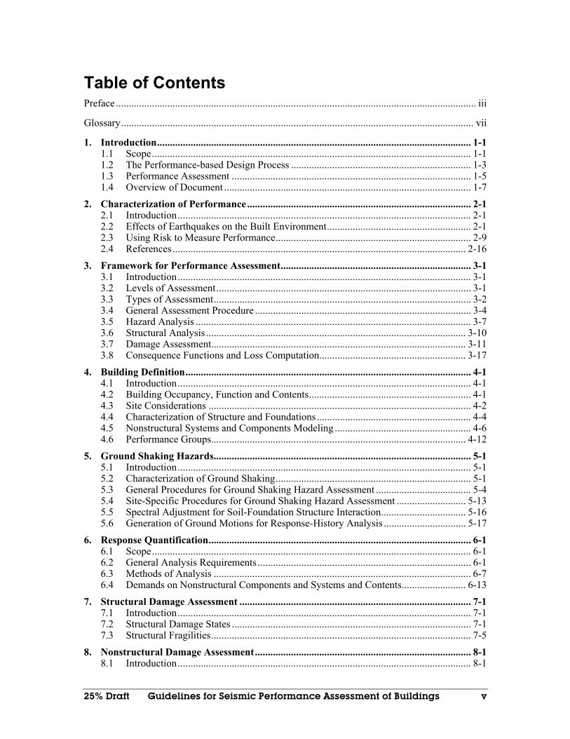
Table of Contents Preface ............................................................................................................................................ iii
Glossary......................................................................................................................................... vii
1. Introduction.......................................................................................................................... 1-1 1.1 Scope............................................................................................................................ 1-1 1.2 The Performance-based Design Process ...................................................................... 1-3 1.3 Performance Assessment ............................................................................................. 1-5 1.4 Overview of Document ................................................................................................ 1-7
2. Characterization of Performance ....................................................................................... 2-1 2.1 Introduction.................................................................................................................. 2-1 2.2 Effects of Earthquakes on the Built Environment........................................................ 2-1 2.3 Using Risk to Measure Performance............................................................................ 2-9 2.4 References .................................................................................................................. 2-16
3. Framework for Performance Assessment.......................................................................... 3-1 3.1 Introduction.................................................................................................................. 3-1 3.2 Levels of Assessment................................................................................................... 3-1 3.3 Types of Assessment.................................................................................................... 3-2 3.4 General Assessment Procedure .................................................................................... 3-4 3.5 Hazard Analysis ........................................................................................................... 3-7 3.6 Structural Analysis ..................................................................................................... 3-10 3.7 Damage Assessment................................................................................................... 3-11 3.8 Consequence Functions and Loss Computation......................................................... 3-17
4. Building Definition............................................................................................................... 4-1 4.1 Introduction.................................................................................................................. 4-1 4.2 Building Occupancy, Function and Contents............................................................... 4-1 4.3 Site Considerations ...................................................................................................... 4-2 4.4 Characterization of Structure and Foundations............................................................ 4-4 4.5 Nonstructural Systems and Components Modeling ..................................................... 4-6 4.6 Performance Groups................................................................................................... 4-12
5. Ground Shaking Hazards.................................................................................................... 5-1 5.1 Introduction.................................................................................................................. 5-1 5.2 Characterization of Ground Shaking............................................................................ 5-1 5.3 General Procedures for Ground Shaking Hazard Assessment ..................................... 5-4 5.4 Site-Specific Procedures for Ground Shaking Hazard Assessment ........................... 5-13 5.5 Spectral Adjustment for Soil-Foundation Structure Interaction................................. 5-16 5.6 Generation of Ground Motions for Response-History Analysis ................................ 5-17
6. Response Quantification...................................................................................................... 6-1 6.1 Scope............................................................................................................................ 6-1 6.2 General Analysis Requirements ................................................................................... 6-1 6.3 Methods of Analysis .................................................................................................... 6-7 6.4 Demands on Nonstructural Components and Systems and Contents......................... 6-13
7. Structural Damage Assessment .......................................................................................... 7-1 7.1 Introduction.................................................................................................................. 7-1 7.2 Structural Damage States ............................................................................................. 7-1 7.3 Structural Fragilities..................................................................................................... 7-5
8. Nonstructural Damage Assessment.................................................................................... 8-1 8.1 Introduction.................................................................................................................. 8-1

Table of Contents
25% Draft Guidelines for Seismic Performance Assessment of Buildings vi
8.2 Nonstructural Damage States ....................................................................................... 8-1 8.3 Nonstructural Fragilities............................................................................................... 8-3
9. Consequence Functions ....................................................................................................... 9-1 9.1 Introduction.................................................................................................................. 9-1 9.2 Casualty Functions ....................................................................................................... 9-1 9.3 Direct Economic Loss Functions ................................................................................. 9-2 9.4 Downtime Functions .................................................................................................... 9-2
Appendix A. Characteristics of the Lognormal Distribution ............................................ A-1 Appendix B. Performance Groups, Damage States, and Fragilities ..................................B-1
B.1 General .........................................................................................................................B-1 B.2 General Strategy...........................................................................................................B-1 B.3 Damage States and Fragilities ......................................................................................B-2
Appendix C. Developing Fragility Functions for Structural and Nonstructural Components ..................................................................................................... C-1
C.1 Purpose.........................................................................................................................C-1 C.2 Background ..................................................................................................................C-1 C.3 General Procedure........................................................................................................C-3 C.4 Test Protocols...............................................................................................................C-5
Appendix D. Default Damage and Loss Data for Structural Systems .............................. D-1 D.1 General ........................................................................................................................ D-1 D.2 Default Damage and Loss Data for Moment-Resisting Steel Frames......................... D-1 D.3 Default Damage and Loss Data for Light Wood Frame Systems ............................... D-1
Appendix E. Default Nonstructural Performance Group Quantity and Fragility Data for Selected Occupancies ........................................................................E-1
E.1 General .........................................................................................................................E-1 E.2 Default Performance Groups........................................................................................E-1 E.3 Default Performance Group Fragilities ........................................................................E-5 E.4 Component-Specific Fragility Data .............................................................................E-7
Appendix F. Constitutive Relationships for Structural Modeling .....................................F-1 Appendix G. Default Consequence Functions for Structural Systems.............................. G-1 Appendix H. Default Consequence Functions for Building Occupancies......................... H-1 ATC-58 Project Participants .....................................................................................................P-1
25% Draft Guidelines for Seismic Performance Assessment of Buildings vii
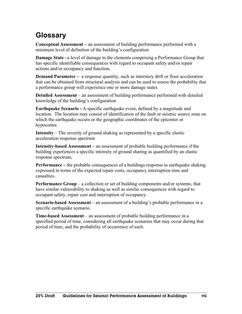
Glossary Conceptual Assessment – an assessment of building performance performed with a minimum level of definition of the building’s configuration
Damage State –a level of damage to the elements comprising a Performance Group that has specific identifiable consequences with regard to occupant safety and/or repair actions and/or occupancy and function.
Demand Parameter – a response quantity, such as interstory drift or floor acceleration that can be obtained from structural analysis and can be used to assess the probability that a performance group will experience one or more damage states
Detailed Assessment – an assessment of building performance performed with detailed knowledge of the building’s configuration
Earthquake Scenario - A specific earthquake event, defined by a magnitude and location. The location may consist of identification of the fault or seismic source zone on which the earthquake occurs or the geographic coordinates of the epicenter or hypocenter.
Intensity – The severity of ground shaking as represented by a specific elastic acceleration response spectrum
Intensity-based Assessment – an assessment of probable building performance if the building experiences a specific intensity of ground sharing as quantified by an elastic response spectrum.
Performance – the probable consequences of a buildings response to earthquake shaking expressed in terms of the expected repair costs, occupancy interruption time and casualties.
Performance Group – a collection or set of building components and/or systems, that have similar vulnerability to shaking as well as similar consequences with regard to occupant safety, repair cost and interruption of occupancy.
Scenario-based Assessment – an assessment of a building’s probable performance in a specific earthquake scenario.
Time-based Assessment – an assessment of probable building performance in a specified period of time, considering all earthquake scenarios that may occur during that period of time, and the probability of occurrence of each.


1. Introduction
25% Draft Guidelines for Seismic Performance Assessment of Buildings 1-1
1 Introduction
1.1 Scope This Recommended Guidelines for Building Seismic Performance Assessment document provides procedures and criteria that can be used to predict the probable earthquake performance of individual buildings. These Guidelines are intended to be used as part of a performance-based seismic design process, either for design of new buildings, or evaluation and upgrade of existing buildings. However, they can be applied to the seismic performance assessment of new or existing buildings, undertaken independent of a design process.
In these Guidelines, performance is measured in terms of the risk of incurring various earthquake-induced losses. Risks considered include loss of life and serious injury, resulting from earthquake-induced damage, i.e. casualties; potential economic loss associated with repair and replacement of damaged systems and components, i.e. direct economic losses; and time of occupancy interruption while a building is inspected for damage, repaired, cleaned up and restored to a state that permits occupancy and use, i.e. downtime. These measures of earthquake performance have been selected as being most relevant to the broad group of decision makers, including building officials, developers, owners, lenders, insurers, tenants and others, who must make decisions as to the acceptable performance for an individual building or broad classes of buildings. Although risks associated with earthquake induced fire, release of hazardous materials, and offsite effects such as disruption utilities, lifelines and other community infrastructure systems may be of interest to some decision makers, these other risks are outside the scope of this guideline document. However the basic procedures presented herein could be extended to encompass these other risks.
Procedures are provided herein for three different types of seismic performance assessments. Intensity-based assessments provide estimates of the probable casualties, direct economic losses and downtime if the building experiences a specific intensity of ground shaking as represented by a defined acceleration response spectrum. Scenario-based assessments provide estimates of the probable casualties, direct economic losses and downtime if the building is subjected to ground shaking resulting from a specified earthquake scenario, defined by a magnitude and distance from the site. Time-based assessments provide estimates of the probability of experiencing a given level of casualties, direct economic losses and downtime, over a specified period of time, considering all earthquakes that may occur in that time, and the probability of each.
Under these Guidelines, the performance assessment process initiates with definition of the building’s composition, its site, its configuration, and identification of its structural and nonstructural systems, their characteristics, their distribution throughout the building, the cost of these features, and their potential impact on building occupancy and life safety. Next, the user must define the seismic environment for the building, either in the form of a specific intensity of ground shaking, for which the assessment will be performed, or hazard data that indicates the probability of experiencing various levels of ground shaking intensity. One or more analytical models are developed to represent critical structural and nonstructural elements and structural analysis is performed to
1. Introduction
1-2 Guidelines for Seismic Performance Assessment of Buildings 25% Draft
quantify the structure’s response to earthquake ground motions and the demands on building nonstructural features. From this determination of structural and nonstructural response, the probable levels of damage sustained by the structural and nonstructural systems is projected and finally, the probable losses, in terms of casualties, direct economic losses and downtime are calculated.
This process inherently incorporates many uncertainties relating to a lack of perfect knowledge of the characteristics of the building itself, the earthquake ground motions it may experience, the response of the building given the ground motions, the damage it will experience given the response and the consequences of this damage with regard to repair cost, repair time and the risks to persons within the building at the time of the earthquake. To properly account for these uncertainties, these Guidelines utilize methods of structural reliability analysis and probabilistic loss evaluation.
Generally, key factors that affect a buildings performance include its structural system type and the kinds of nonstructural systems and components that are present. Buildings having the same structural system will have similar structural damage characteristics and consequences of damage. Similarly, buildings in the same use, for example, healthcare, will have similar types of nonstructural systems and components, and therefore similar damageability of their nonstructural features. Since the data required to perform reliable assessments of the many types of structural systems and uses common in the building inventory is not presently available, the guidelines presented herein include an overall framework for the performance assessment process and detailed data for a subset of selected building types, where a building type is defined by a structural system type and by a primary use (or uses), for example, steel moment frame office building. In addition, procedures are provided to develop the needed data for other structural systems and building uses.
This edition of the Guidelines contains data specific to buildings constructed using the structural systems listed in Table 1-1 and the building uses listed in Table 1-2. It is expected that these Guidelines will be revised periodically to incorporate new information on additional structural systems and building uses as such data become available.
Table 1-1 Structural Systems Included In Guidelines
Light wood frame
Moment-resisting steel frame
Table 1-2 Building Uses Included in Guidelines
Commercial office Multifamily residential
Education Research
Healthcare Retail
Hospitality Warehouse
Several potential uses are anticipated for these Guidelines. Individual structural engineers can apply these Guidelines to the seismic performance assessment and upgrade design of
1. Introduction
25% Draft Guidelines for Seismic Performance Assessment of Buildings 1-3
existing buildings or the seismic design of new buildings. Suppliers of building products, including architectural, mechanical, electrical and structural systems and components can use these Guidelines to quantify the performance capability of their products. Developers of building codes and design standards can use these Guidelines to evaluate the effectiveness of current prescriptive design standards and to make improvements to these standards. Educators can use these Guidelines as instructional materials in engineering curricula. Researchers may find these Guidelines helpful in identifying areas where additional building performance research is needed.
These Guidelines have been prepared by the Applied Technology Council, under its ATC-58 project to develop Next-generation Performance-based Seismic Design Criteria. Funding for this project has been primarily been provided by the Federal Emergency Management Agency of the Department of Homeland Security.
1.2 The Performance-based Design Process Performance-based design is a process that explicitly considers the way a building is likely to perform, as its design features are determined. Most building design conducted today is not performance-based, but instead, is conducted to conform to prescriptive criteria contained in the building codes. These prescriptive criteria regulate the acceptable materials of construction, structural systems, required structural strength and stiffness, and even small details as to how the structure is constructed. Although these prescriptive criteria are intended to result in buildings capable of providing certain levels of performance, the performance capability of the individual building designs are never assessed as part of the code design process to determine if the building will be able to provide the desired performance. As a result, the performance capability of buildings designed to the prescriptive criteria is highly variable and for a given building, not specifically known. Some buildings designed to the prescriptive criteria will perform much better than the minimum standard while the performance of other buildings will be worse.
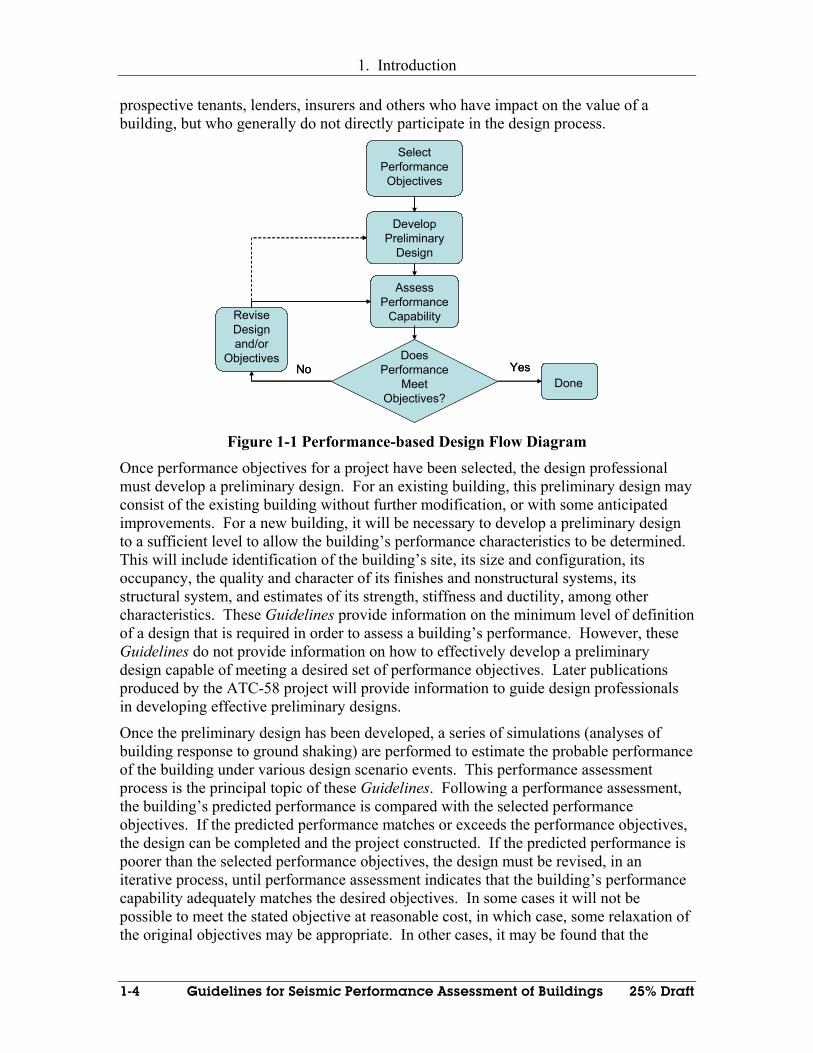
In the performance-based design process, the performance capability of a building is identified as an inherent part of the design process and guides the many design decisions that must be made. Figure 1-1 is a flowchart that presents the key steps in the performance-based design process.
The process initiates with design criteria selection. Design criteria are stated in the form of one or more performance objectives. Each performance objective is a statement of the acceptable risk of incurring damage of different amounts and the consequential losses that occur as a result of this damage. In these Guidelines, performance objectives are specifically stated in terms of the acceptable risk of casualties, direct economic losses, and downtime, resulting from earthquake-induced damage. These acceptable risks can be expressed for specific levels of earthquake ground motion intensity, for different scenario earthquakes or for a specific period of time, considering all of the earthquakes that can occur during that time period and the probability of their occurrence. Generally, a team of decision makers, including the building owner, the design professionals and the building official, will participate in selecting the performance objectives for a building. This team may consider the needs and desires of a wider group of stakeholders including
1. Introduction
1-4 Guidelines for Seismic Performance Assessment of Buildings 25% Draft
prospective tenants, lenders, insurers and others who have impact on the value of a building, but who generally do not directly participate in the design process.
SelectPerformanceObjectives
DevelopPreliminary
Design
AssessPerformance
Capability
DoesPerformance
MeetObjectives?
ReviseDesignand/or
ObjectivesNo
DoneYes
SelectPerformanceObjectives
DevelopPreliminary
Design
AssessPerformance
Capability
DoesPerformance
MeetObjectives?
ReviseDesignand/or
ObjectivesNo
DoneYes
Figure 1-1 Performance-based Design Flow Diagram
Once performance objectives for a project have been selected, the design professional must develop a preliminary design. For an existing building, this preliminary design may consist of the existing building without further modification, or with some anticipated improvements. For a new building, it will be necessary to develop a preliminary design to a sufficient level to allow the building’s performance characteristics to be determined. This will include identification of the building’s site, its size and configuration, its occupancy, the quality and character of its finishes and nonstructural systems, its structural system, and estimates of its strength, stiffness and ductility, among other characteristics. These Guidelines provide information on the minimum level of definition of a design that is required in order to assess a building’s performance. However, these Guidelines do not provide information on how to effectively develop a preliminary design capable of meeting a desired set of performance objectives. Later publications produced by the ATC-58 project will provide information to guide design professionals in developing effective preliminary designs.
Once the preliminary design has been developed, a series of simulations (analyses of building response to ground shaking) are performed to estimate the probable performance of the building under various design scenario events. This performance assessment process is the principal topic of these Guidelines. Following a performance assessment, the building’s predicted performance is compared with the selected performance objectives. If the predicted performance matches or exceeds the performance objectives, the design can be completed and the project constructed. If the predicted performance is poorer than the selected performance objectives, the design must be revised, in an iterative process, until performance assessment indicates that the building’s performance capability adequately matches the desired objectives. In some cases it will not be possible to meet the stated objective at reasonable cost, in which case, some relaxation of the original objectives may be appropriate. In other cases, it may be found that the
1. Introduction
25% Draft Guidelines for Seismic Performance Assessment of Buildings 1-5
building is inherently capable of performance superior to that required by the performance objectives and that because of other design considerations, it can not practically be designed to reduce its probable performance. In such cases, the superior performance capability should be documented and accepted.
1.3 Performance Assessment The process of performance assessment is inherently uncertain and requires that a number of assumptions be made as to the severity and character of earthquake shaking the building may experience in the future, the condition and occupancy of the building at the time an earthquake occurs and the efficiency with which tenants, owners, design professionals and contractors are able to respond and repair the building and restore it to service, once damage occurs. The procedures contained in these Guidelines directly consider the effect of these uncertainties and our lack of definitive knowledge or our ability to predict actual future performance. Under these Guidelines, performance can be expressed in a number of ways that consider these uncertainties including:
• “median” estimates. These estimates are made at the 50% confidence level. That is, there is as much chance that the actual performance will actually be better than indicated, as there is that it will be worse.
• “mean” estimates. These estimates are average estimates. If the building, or a number of buildings that are similar to it, experience a number of events of similar severity, the mean estimate should provide a close approximation of the average performance outcome from these various events.
• “specified-confidence” estimates. These estimates are expressed together with a statement of the confidence level that the stated loss will not be exceeded. An example is the so-called Probable Maximum Loss (PML), which, is an estimate of probable direct economic loss having a 90% confidence of not being exceeded.
• “bounded” estimates. These estimates express the probable ranges of loss that could occur within some stated confidence limits.
In addition to these choices as to the level of confidence associated with a performance assessment, these Guidelines also permit choices with regard to the earthquake environment for which an assessment is made. Choices include:
• “intensity-based” assessments in which the probable performance of the building is determined for a specific intensity of ground shaking, typically characterized by an elastic ground shaking response spectrum
• “scenario-based” assessments in which the probable performance of the building is determined for a specific scenario earthquake, characterized by a particular magnitude earthquake occurring along a specified fault or at a specified distance form the site
• “time-based” assessments in which the probable performance of the building is determined for a specified period of time, for example 1 year, 5-years, 30-years, etc, as best suits the need of the decision makers, considering all
1. Introduction
1-6 Guidelines for Seismic Performance Assessment of Buildings 25% Draft
earthquake scenarios that may occur in that period and the probability that each such scenario may occur
These options as to the type of performance assessment generated may be combined in a variety of ways. Thus, intensity-based, scenario-based and time-based assessments can all be generated with any desired confidence level including mean and median levels of confidence.
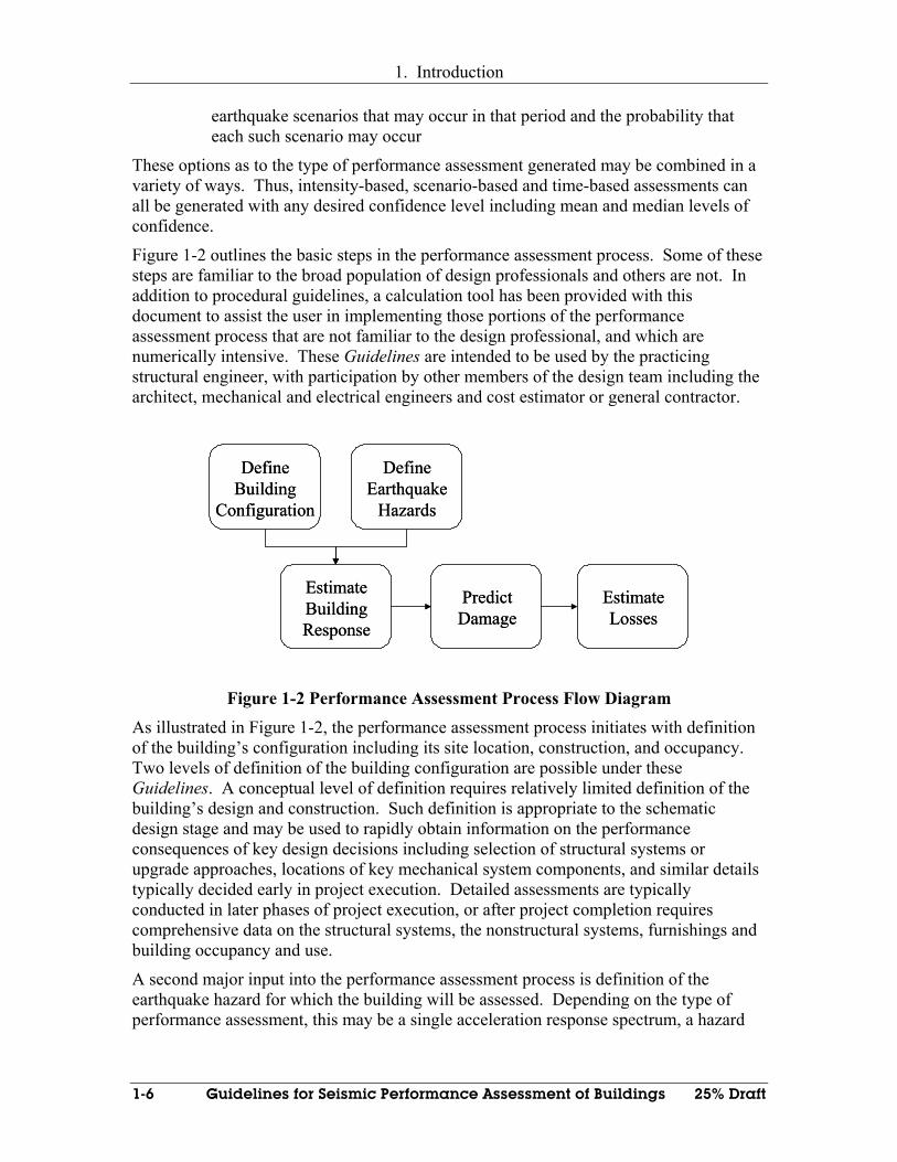
Figure 1-2 outlines the basic steps in the performance assessment process. Some of these steps are familiar to the broad population of design professionals and others are not. In addition to procedural guidelines, a calculation tool has been provided with this document to assist the user in implementing those portions of the performance assessment process that are not familiar to the design professional, and which are numerically intensive. These Guidelines are intended to be used by the practicing structural engineer, with participation by other members of the design team including the architect, mechanical and electrical engineers and cost estimator or general contractor.
DefineBuilding
Configuration
DefineEarthquake
Hazards
EstimateBuildingResponse
PredictDamage
EstimateLosses
DefineBuilding
Configuration
DefineEarthquake
Hazards
EstimateBuildingResponse
PredictDamage
EstimateLosses
Figure 1-2 Performance Assessment Process Flow Diagram As illustrated in Figure 1-2, the performance assessment process initiates with definition of the building’s configuration including its site location, construction, and occupancy. Two levels of definition of the building configuration are possible under these Guidelines. A conceptual level of definition requires relatively limited definition of the building’s design and construction. Such definition is appropriate to the schematic design stage and may be used to rapidly obtain information on the performance consequences of key design decisions including selection of structural systems or upgrade approaches, locations of key mechanical system components, and similar details typically decided early in project execution. Detailed assessments are typically conducted in later phases of project execution, or after project completion requires comprehensive data on the structural systems, the nonstructural systems, furnishings and building occupancy and use.
A second major input into the performance assessment process is definition of the earthquake hazard for which the building will be assessed. Depending on the type of performance assessment, this may be a single acceleration response spectrum, a hazard
1. Introduction
25% Draft Guidelines for Seismic Performance Assessment of Buildings 1-7
curve indicating the severity of various intensities of shaking, suites of ground motions representative of the various shaking levels, or combinations of these.
Following definition of the building performance characteristics and seismic hazard, the structural engineer must develop an analytical model of the structure and key nonstructural systems and components. This model is used to perform structural analyses to predict the building’s response to the ground shaking. These analyses provide statistical data on building drifts, floor accelerations, member forces and deformations, termed demand parameters, at different levels of ground shaking intensity.
Building drift, floor acceleration, and other demand data from the structural analyses and data on the building configuration is used to calculate the possible distribution of damage to structural and nonstructural building components and also the potential distribution in casualty, economic and occupancy losses. To assist with these calculations, a calculation tool is provided with these Guidelines. This calculation tool can utilize damageability data contained within a default database or users can supplement this data with component-specific information obtained from product suppliers, testing laboratories and other sources.
The performance assessment produces probability distribution functions for casualties, repair costs and occupancy interruption time. From these distributions it is possible to extract the expected losses at various confidence levels, as previously described. Further, it is possible to identify the most significant contributors to these losses, to guide design decisions intended to reduce the severity of assessed losses.
1.4 Overview of Document Chapter 2 of this document presents a more detailed discussion of the overall performance assessment process used in these Guidelines as well as discussion of the benefits of this approach relative to that used in earlier performance-based design approaches. Chapter 3 provides a detailed description of the various steps in the performance assessment process and directs users to other sections of this document for specific instructions on how to implement one specific procedure for making the calculations described above.
Chapter 4 provides guidelines for developing the building performance model for a project, including definition of structural and nonstructural building components. Chapter 5 provides guidelines for determining and quantifying seismic hazards and selecting and scaling ground motions used as input to the performance assessment process.
Chapter 6 provides guidelines for structural analysis. Structural analysis is used to predict the response of the structure and the demands on the nonstructural elements and components. Chapter 7 presents the procedures for developing either building-specific or standardized structural damage and loss functions for building structures. It also includes description of the default structural damage and loss functions contained in the performance assessment calculation tool for selected structural systems. Chapter 8 provides guidelines for defining nonstructural components of buildings and characterizing their performance. Chapter 9 provides information needed to translate

1. Introduction
1-8 Guidelines for Seismic Performance Assessment of Buildings 25% Draft
estimated damage into a measure of loss (i.e. casualties, direct economic loss, downtime) using consequence functions.
Detailed data needed to support the application of this methodology is generally contained in appendices. Appendix A presents information on lognormal distributions, used throughout these Guidelines to characterize uncertainty. Appendix B presents information on how to form the constituent parts of a building into performance groups that are used to characterize damage. Appendix C presents information on the development of fragility relations for building components. Appendix D presents default performance groups and fragility data for selected structural systems. Appendix E presents default performance groups and fragility data for nonstructural components in selected building occupancies. Appendix F provides constitutive relationships for structural modeling.
Reader Note: Appendix F is not presently developed, but will be provided in later drafts of the Guidelines.

25% Draft Guidelines for Seismic Performance Assessment of Buildings 2-1
2 Characterization of Performance
2.1 Introduction This section introduces the concept of using the risk of incurring some basic losses (i.e. casualties, direct economic losses, and downtime) to measure the seismic performance of buildings. This concept is developed in Section 2.2 by considering the effects of earthquakes on the built environment in general and with respect to individual buildings (Section 2.2.1). Two primary factors control the performance of buildings in earthquakes: the intensity of shaking and the capability of the building to sustain this shaking with controlled levels of damage (Section 2.2.2). Traditional code procedures address these two factors with pass-fail prescriptive procedures. Recent developments in performance-based design add some important new information to the design process. Both of these approaches are reviewed in Section 2.2.3. The risk analysis procedures embedded in these Guidelines are inherent to the performance-based design process and can further enhance information available for design (Section 2.2.4). Section 2.2.5 presents a theoretical framework that forms the basis of the assessment procedures presented in these Guidelines.
The procedures presented in these Guidelines represent a new approach to performance-based engineering. Development of this new approach, using risk to characterize the performance of buildings in extreme events, satisfies two important requirements. First, the procedures are technically sound and conducive to engineering calculations and manipulations. This requires quantitative, as opposed to qualitative, parameters and relationships. Sections 2.3.1 to 2.3.4 present the conceptual technical considerations and processes. The results of the performance assessment process are basic risk parameters (e.g. mean annualized casualties, direct economic losses, and downtime from seismic shaking) that are specifically associated with a building, or the proposed design of a building, located on a specific site. Groups or individuals who are not engineers often make important decisions about buildings subject to extreme events. Many have well-established ways of evaluating alternatives in their own vernacular. Consequently, the second important requirement is that the technical data from the engineering analysis must be readily adaptable to serve a variety of practical needs. The adaptation of the basic risk parameters to suit a variety of practical needs is the subject of Section 2.3.5.
2.2 Effects of Earthquakes on the Built Environment Earthquakes, as well as many other hazards including high winds, wild lands fires, and floods, are natural phenomena. Although these events are inexorable over time, they do not alone cause losses in communities. Communities and the related built environment can be more or less vulnerable to natural disasters. As a result of the tsunami of 2004, thousands in coastal villages perished primarily because of their location in low-lying coastal planes, where they could be inundated. If these communities had been constructed on higher ground, the mass loss of life and property may not have occurred. Effective planning and design can mitigate losses. This section describes the effects of

2. Characterization of Performance
2-2 Guidelines for Seismic Performance Assessment of Buildings 25% Draft
earthquakes on building structures and the factors that determine how severe these effects are in terms of the losses sustained.
2.2.1 Earthquake Effects on Buildings The primary earthquake effect of interest is the potential impact on human safety, i.e. the number of deaths and serious injuries that may occur as a result of earthquake-induced damage to buildings. However, even in the fortunate situations when no one is hurt, earthquakes still cause serious damage to buildings and the loss of functions they serve. Earthquake shaking can potentially completely destroy a facility, depending on the specific vulnerability of the affected building and intensity of the event. The risk of deaths and injuries at an electrical substation may be quite small, as few people are typically present in such facilities, yet the loss of equipment and services that results from damage can be important and costly both to the operator of the facility and to the region that relies on the substation for power. Even for low intensity motions, economic impacts, in terms of direct economic losses and those associated with impeded function of facilities, can be significant. Beyond the direct economic losses at an individual facility, consequences extend to the broader social and economic community (e.g., loss of power serving a major industrial complex). These Guidelines categorize the potential effects of earthquakes in terms of:
• Human losses (deaths and serious injuries), herein termed casualties
• Direct economic losses associated with damage to the building and its contents, herein termed direct economic loss, and
• Losses resulting from the impediments to use of a building after an earthquake, herein termed downtime.
2.2.2 Factors Affecting Performance The performance of a building in an earthquake in terms of the nature and scope of the potential losses, as outlined in the previous section, depends on two fundamental considerations.
The first of these is the intensity of the ground shaking. This can be visualized by imagining the results of the inspection of a given building after an earthquake event. If the shaking intensity was relatively slight, the building structure may have responded elastically. Perhaps no one was hurt and damage was limited to that considered cosmetic and inexpensive and that can be repaired without shutting the building down. If the shaking was more intense, the structure may have responded inelastically causing more serious and expensive damage. Some of the occupants may have suffered injuries from falling debris. The building might be “red tagged” as unfit for occupancy until structural repairs are made. If the ground shaking were extreme, portions of the building structure may have collapsed resulting in deaths and serious injuries. Such damage could be so heavy as to make repair infeasible and uneconomical compared to demolition and replacement.
The intensity of shaking at a given building site depends on a number of parameters including:
2. Characterization of Performance
25% Draft Guidelines for Seismic Performance Assessment of Buildings 2-3
• Type of fault on which the earthquake originated (e.g strike-slip, thrust, subduction).
• Length,depth, and direction of rupture.
• Surface roughness of the rupture plane.
• Distance of the rupture from the site.
• Subsurface conditions along the travel path from the rupture to the site.
• Regional geology in the vicinity of the site (e.g. the presence of sedimentary basins, or subsurface strata that can reflect and refract the seismic waves).
• Site soils conditions.
• Site topography (e.g. location atop, or at the foot of, a hill).
The second fundamental factor controlling the effects of earthquakes is the vulnerability of the building itself. Imagine the effects of earthquake shaking of a single intensity on different types of buildings. A new base-isolated hospital, may experience virtually no damage and be ready to provide emergency services to the community. A wood frame house may sustain some broken windows and cracked partitions. The residents probabaly are not injured and the minor repairs required can probably be made while they continue to occupy the house. Those living in an older unreinforced masonry building may not fare as well. A parapet may collapse and severely injure several people. Major cracks may form in the load bearing walls resulting in concern for stability of the building in aftershocks. The residents may be evacuated and in need of alternative housing as the building is demolished. A light, steel, braced frame building subject to the same shaking may survive with no structural damage, yet the contents of the building used to manufacture expensive computer components are severely disrupted and damaged. It may take months or years to replace some of this damaged equipment. In the meantime, a large amount of revenue will be lost due to an inability of the tenant to produce computer components until the new equipment is procured and installed.
Characteristics of buildings pertinent to their vulnerability to earthquakes include:
• Basement and foundation conditions.
• Type of structural system, the strength and stiffness of the structure and details of construction.
• Condition of structure with respect to maintenance and previous damage or deteriorization.
• The type and quality of architectural, mechanical, electrical and plumbing systems, and the extent that their installation included provision for seismic protection.
2. Characterization of Performance
2-4 Guidelines for Seismic Performance Assessment of Buildings 25% Draft
• The types of contents , and how they are installed.
• Functional use of the building.
• Number of occupants present at the time of the earthquake and their location in the building.
• Vulnerability of off site utilities.
• Local and regional economic conditions.
2.2.3 Design considerations Planning and design decisions can affect both the intensity of shaking of a building and the vulnerability of a building. The intensity of motion is largely a function of its site location. In most instances, considerations that supersede seismic concerns dictate the selection of the building site for new buildings, and for existing buildings, the selection of an alternative site is not typically a practical consideration. Consequently, the discussion here focuses on controlling the vulnerability of a building at a given site.
Standards for the design of buildings to resist the effects of earthquakes first appeared in the United States, nearly one hundred years ago following the San Francisco Earthquake of 1906. Over the years, building codes in the U.S. and elsewhere have evolved based primarily on observed damage in subsequent earthquakes, as well as empirical and theoretical research results. The traditional code format has been prescriptive. Codes require that the design conform to a set of specific criteria governing the structural systems, materials of construction, strength, and details of construction. In the past ten to fifteen years, performance-based design has evolved as a new approach to design to resist the effects of extreme events, including earthquakes. Performance-based design differs from the prescriptive approach by focusing on the assessment of consequences of an extreme event for a given design, rather than strictly meeting prescriptive criteria. The engineer modifies the design, and assesses the likely performance of the design until the performance is deemed acceptable.
2.2.3.1 Prescriptive code approach
Conventional building codes (NEHRP, ICC) consider both of the fundamental factors affecting building performance in earthquakes discussed in the previous section for design purposes.
Based on the location of the building the code specifies the intensity of shaking to be used for design in the form of a response spectrum relating peak spectral acceleration to the period of the building. The design spectrum represents shaking with a relatively low probability of being exceeded in the lifetime of a typical building. The design spectrum is the result of prescribed parameters that reflect local soils conditions and the proximity of active faults.
In order to assess the vulnerability of an existing building or a design, the engineer models the structural characteristics of the building’s primary lateral force resisting elements. Normally the model reflects the assumption that the building response will
2. Characterization of Performance
25% Draft Guidelines for Seismic Performance Assessment of Buildings 2-5
remain elastic. This is unrealistic for most buildings subject to ground shaking of design-level intensity. Consequently, the code specifies a reduction in the forces applied to the model to reflect the observed capability of certain structural systems to resist ground shaking without collapse. The reduction reflects the capability (i.e. ductility) of different structural systems to sustain inelastic deformations with out adverse behavior. The results of the structural analysis are forces and displacements (i.e. demands) in the individual components of the structure that the engineer compares to acceptance criteria, consisting of permissible strengths and interstory drift ratios. In addition, the code prescribes many details for construction (e.g. requirements to confine concrete with transverse reinforcing when inelastic deformations are anticipated).
In summary, traditional codes for seismic design comprise a checklist of pass-fail requirements that must be satisfied for compliance. The design procedure itself does not produce an assessment of the likely effects of actual earthquakes and the resulting performance of the specific building in terms of losses is not explicitly determined. From a building owner’s perspective the prescriptive code approach simplifies the design process. If a building is code-compliant, most owners assume that the seismic performance of the building will be acceptable, without understanding what the performance actually might be. This often leads to disappointment, after an earthquake, when owners and tenants discover that “acceptable performance” includes the potential for significant damage and loss of occupancy. Many owners whose buildings suffered damage during the Northridge Earthquake, for example, expressed outrage and a belief that because their buildings were code-compliant, they were also earthquake-proof.
2.2.3.2 First Generation Performance-based Design Procedures
Recent development of performance-based design guidelines and standards such as the FEMA 356 Prestandard and Commentary for the Seismic Rehabilitation of Buildings (ASCE, 2000), and ATC 40 Seismic Evaluation and Retrofit of Concrete Buildings (ATC, 1996) address some of the shortcomings of prescriptive design procedures. The performance-based approach uses engineering analysis techniques, sometimes termed simulation, to estimate the potential effects of seismic shaking on buildings in a measurable manner. Similar procedures using advanced analytical techniques have been used for years in the automotive and aircraft industries for the design of prototypes that will eventually be mass-produced. Recent advances in structural engineering and information technology are reducing the effort and costs of these techniques such that they can be applied practically on a more widespread basis to the design of individual buildings.
Performance-based procedures express the intensity of an earthquake explicitly in quantifiable engineering terms. For example, an earthquake of a certain magnitude and location would result in shaking at a building site with an intensity characterized by a record of actual ground movement or a derivative parameter (e.g. peak ground acceleration, peak acceleration at the period of the structure). Alternatively, the intensity can be specified probabilistically as a level of shaking expected within a time period (e.g. 500 year event, 100 year event). This probabilistic characterization is analogous to that often used for wind or flood.
2. Characterization of Performance
2-6 Guidelines for Seismic Performance Assessment of Buildings 25% Draft
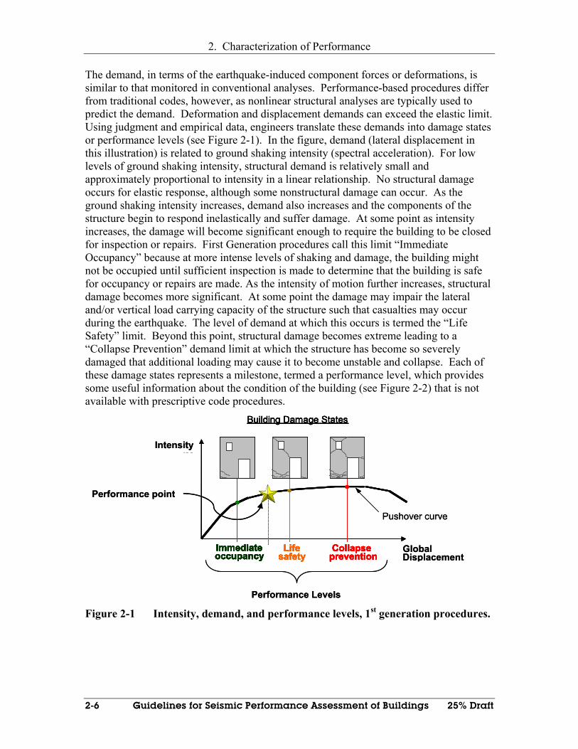
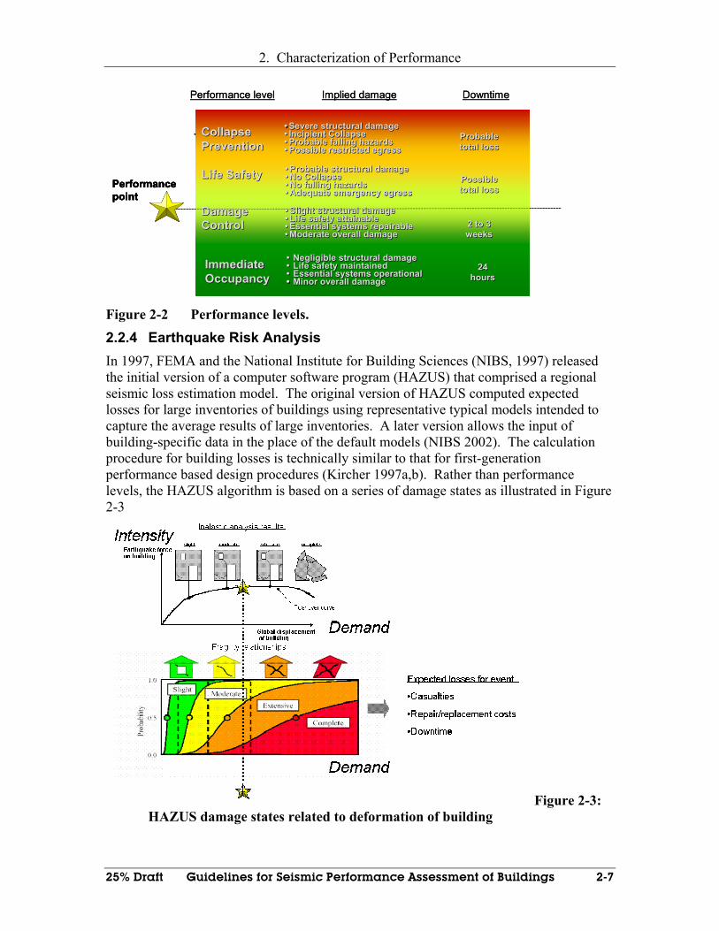
The demand, in terms of the earthquake-induced component forces or deformations, is similar to that monitored in conventional analyses. Performance-based procedures differ from traditional codes, however, as nonlinear structural analyses are typically used to predict the demand. Deformation and displacement demands can exceed the elastic limit. Using judgment and empirical data, engineers translate these demands into damage states or performance levels (see Figure 2-1). In the figure, demand (lateral displacement in this illustration) is related to ground shaking intensity (spectral acceleration). For low levels of ground shaking intensity, structural demand is relatively small and approximately proportional to intensity in a linear relationship. No structural damage occurs for elastic response, although some nonstructural damage can occur. As the ground shaking intensity increases, demand also increases and the components of the structure begin to respond inelastically and suffer damage. At some point as intensity increases, the damage will become significant enough to require the building to be closed for inspection or repairs. First Generation procedures call this limit “Immediate Occupancy” because at more intense levels of shaking and damage, the building might not be occupied until sufficient inspection is made to determine that the building is safe for occupancy or repairs are made. As the intensity of motion further increases, structural damage becomes more significant. At some point the damage may impair the lateral and/or vertical load carrying capacity of the structure such that casualties may occur during the earthquake. The level of demand at which this occurs is termed the “Life Safety” limit. Beyond this point, structural damage becomes extreme leading to a “Collapse Prevention” demand limit at which the structure has become so severely damaged that additional loading may cause it to become unstable and collapse. Each of these damage states represents a milestone, termed a performance level, which provides some useful information about the condition of the building (see Figure 2-2) that is not available with prescriptive code procedures.
GlobalDisplacementParameter(EDP)
Pushover curve
Building Damage States
Immediateoccupancy
Lifesafety
Collapseprevention
Performance Levels
Building Damage States
ImmediateoccupancyImmediateoccupancy
LifesafetyLife
safetyCollapse
preventionCollapse
prevention
Intensity measure, IM
Performance point
GlobalDisplacementParameter(EDP)
Pushover curve
Building Damage States
ImmediateoccupancyImmediateoccupancy
LifesafetyLife
safetyCollapse
preventionCollapse
prevention
Performance Levels
Building Damage States
ImmediateoccupancyImmediateoccupancy
LifesafetyLife
safetyCollapse
preventionCollapse
prevention
Intensity measure, IM
Performance point
Figure 2-1 Intensity, demand, and performance levels, 1st generation procedures.
2. Characterization of Performance
25% Draft Guidelines for Seismic Performance Assessment of Buildings 2-7
ImmediateOccupancyImmediateOccupancy
•• Negligible structural damageNegligible structural damage•• Life safety maintainedLife safety maintained•• Essential systems operationalEssential systems operational•• Minor overall damageMinor overall damage
2424hourshours
DamageDamageControlControl
•• Slight structural damageSlight structural damage•• Life safety attainableLife safety attainable•• Essential systems repairableEssential systems repairable•• Moderate overall damageModerate overall damage
2 to 32 to 3weeksweeks
Life SafetyLife Safety •• Probable structural damageProbable structural damage•• No CollapseNo Collapse•• No falling hazardsNo falling hazards•• Adequate emergency egressAdequate emergency egress
PossiblePossibletotal losstotal loss
Collapse PreventionCollapse Prevention
•• Severe structural damageSevere structural damage•• Incipient CollapseIncipient Collapse•• Probable falling hazardsProbable falling hazards•• Possible restricted egressPossible restricted egress
ProbableProbabletotal losstotal loss
ImmediateOccupancyImmediateOccupancy
•• Negligible structural damageNegligible structural damage•• Life safety maintainedLife safety maintained•• Essential systems operationalEssential systems operational•• Minor overall damageMinor overall damage
2424hourshours
ImmediateOccupancyImmediateOccupancy
•• Negligible structural damageNegligible structural damage•• Life safety maintainedLife safety maintained•• Essential systems operationalEssential systems operational•• Minor overall damageMinor overall damage
2424hourshours
DamageDamageControlControl
•• Slight structural damageSlight structural damage•• Life safety attainableLife safety attainable•• Essential systems repairableEssential systems repairable•• Moderate overall damageModerate overall damage
2 to 32 to 3weeksweeks
DamageDamageControlControl
•• Slight structural damageSlight structural damage•• Life safety attainableLife safety attainable•• Essential systems repairableEssential systems repairable•• Moderate overall damageModerate overall damage
2 to 32 to 3weeksweeks
Life SafetyLife Safety •• Probable structural damageProbable structural damage•• No CollapseNo Collapse•• No falling hazardsNo falling hazards•• Adequate emergency egressAdequate emergency egress
PossiblePossibletotal losstotal loss
Life SafetyLife Safety •• Probable structural damageProbable structural damage•• No CollapseNo Collapse•• No falling hazardsNo falling hazards•• Adequate emergency egressAdequate emergency egress
PossiblePossibletotal losstotal loss
Collapse PreventionCollapse Prevention
•• Severe structural damageSevere structural damage•• Incipient CollapseIncipient Collapse•• Probable falling hazardsProbable falling hazards•• Possible restricted egressPossible restricted egress
ProbableProbabletotal losstotal loss
Collapse PreventionCollapse Prevention
•• Severe structural damageSevere structural damage•• Incipient CollapseIncipient Collapse•• Probable falling hazardsProbable falling hazards•• Possible restricted egressPossible restricted egress
ProbableProbabletotal losstotal loss
Performance point
ImmediateOccupancyImmediateOccupancy
•• Negligible structural damageNegligible structural damage•• Life safety maintainedLife safety maintained•• Essential systems operationalEssential systems operational•• Minor overall damageMinor overall damage
2424hourshours
DamageDamageControlControl
•• Slight structural damageSlight structural damage•• Life safety attainableLife safety attainable•• Essential systems repairableEssential systems repairable•• Moderate overall damageModerate overall damage
2 to 32 to 3weeksweeks
Life SafetyLife Safety •• Probable structural damageProbable structural damage•• No CollapseNo Collapse•• No falling hazardsNo falling hazards•• Adequate emergency egressAdequate emergency egress
PossiblePossibletotal losstotal loss
Collapse PreventionCollapse Prevention
•• Severe structural damageSevere structural damage•• Incipient CollapseIncipient Collapse•• Probable falling hazardsProbable falling hazards•• Possible restricted egressPossible restricted egress
ProbableProbabletotal losstotal loss
ImmediateOccupancyImmediateOccupancy
•• Negligible structural damageNegligible structural damage•• Life safety maintainedLife safety maintained•• Essential systems operationalEssential systems operational•• Minor overall damageMinor overall damage
2424hourshours
ImmediateOccupancyImmediateOccupancy
•• Negligible structural damageNegligible structural damage•• Life safety maintainedLife safety maintained•• Essential systems operationalEssential systems operational•• Minor overall damageMinor overall damage
2424hourshours
DamageDamageControlControl
•• Slight structural damageSlight structural damage•• Life safety attainableLife safety attainable•• Essential systems repairableEssential systems repairable•• Moderate overall damageModerate overall damage
2 to 32 to 3weeksweeks
DamageDamageControlControl
•• Slight structural damageSlight structural damage•• Life safety attainableLife safety attainable•• Essential systems repairableEssential systems repairable•• Moderate overall damageModerate overall damage
2 to 32 to 3weeksweeks
Life SafetyLife Safety •• Probable structural damageProbable structural damage•• No CollapseNo Collapse•• No falling hazardsNo falling hazards•• Adequate emergency egressAdequate emergency egress
PossiblePossibletotal losstotal loss
Life SafetyLife Safety •• Probable structural damageProbable structural damage•• No CollapseNo Collapse•• No falling hazardsNo falling hazards•• Adequate emergency egressAdequate emergency egress
PossiblePossibletotal losstotal loss
Collapse PreventionCollapse Prevention
•• Severe structural damageSevere structural damage•• Incipient CollapseIncipient Collapse•• Probable falling hazardsProbable falling hazards•• Possible restricted egressPossible restricted egress
ProbableProbabletotal losstotal loss
Collapse PreventionCollapse Prevention
•• Severe structural damageSevere structural damage•• Incipient CollapseIncipient Collapse•• Probable falling hazardsProbable falling hazards•• Possible restricted egressPossible restricted egress
ProbableProbabletotal losstotal loss
Performance point
Performance level Implied damage Downtime
ImmediateOccupancyImmediateOccupancy
•• Negligible structural damageNegligible structural damage•• Life safety maintainedLife safety maintained•• Essential systems operationalEssential systems operational•• Minor overall damageMinor overall damage
2424hourshours
DamageDamageControlControl
•• Slight structural damageSlight structural damage•• Life safety attainableLife safety attainable•• Essential systems repairableEssential systems repairable•• Moderate overall damageModerate overall damage
2 to 32 to 3weeksweeks
Life SafetyLife Safety •• Probable structural damageProbable structural damage•• No CollapseNo Collapse•• No falling hazardsNo falling hazards•• Adequate emergency egressAdequate emergency egress
PossiblePossibletotal losstotal loss
Collapse PreventionCollapse Prevention
•• Severe structural damageSevere structural damage•• Incipient CollapseIncipient Collapse•• Probable falling hazardsProbable falling hazards•• Possible restricted egressPossible restricted egress
ProbableProbabletotal losstotal loss
ImmediateOccupancyImmediateOccupancy
•• Negligible structural damageNegligible structural damage•• Life safety maintainedLife safety maintained•• Essential systems operationalEssential systems operational•• Minor overall damageMinor overall damage
2424hourshours
ImmediateOccupancyImmediateOccupancy
•• Negligible structural damageNegligible structural damage•• Life safety maintainedLife safety maintained•• Essential systems operationalEssential systems operational•• Minor overall damageMinor overall damage
2424hourshours
DamageDamageControlControl
•• Slight structural damageSlight structural damage•• Life safety attainableLife safety attainable•• Essential systems repairableEssential systems repairable•• Moderate overall damageModerate overall damage
2 to 32 to 3weeksweeks
DamageDamageControlControl
•• Slight structural damageSlight structural damage•• Life safety attainableLife safety attainable•• Essential systems repairableEssential systems repairable•• Moderate overall damageModerate overall damage
2 to 32 to 3weeksweeks
Life SafetyLife Safety •• Probable structural damageProbable structural damage•• No CollapseNo Collapse•• No falling hazardsNo falling hazards•• Adequate emergency egressAdequate emergency egress
PossiblePossibletotal losstotal loss
Life SafetyLife Safety •• Probable structural damageProbable structural damage•• No CollapseNo Collapse•• No falling hazardsNo falling hazards•• Adequate emergency egressAdequate emergency egress
PossiblePossibletotal losstotal loss
Collapse PreventionCollapse Prevention
•• Severe structural damageSevere structural damage•• Incipient CollapseIncipient Collapse•• Probable falling hazardsProbable falling hazards•• Possible restricted egressPossible restricted egress
ProbableProbabletotal losstotal loss
Collapse PreventionCollapse Prevention
•• Severe structural damageSevere structural damage•• Incipient CollapseIncipient Collapse•• Probable falling hazardsProbable falling hazards•• Possible restricted egressPossible restricted egress
ProbableProbabletotal losstotal loss
Performance point
ImmediateOccupancyImmediateOccupancy
•• Negligible structural damageNegligible structural damage•• Life safety maintainedLife safety maintained•• Essential systems operationalEssential systems operational•• Minor overall damageMinor overall damage
2424hourshours
DamageDamageControlControl
•• Slight structural damageSlight structural damage•• Life safety attainableLife safety attainable•• Essential systems repairableEssential systems repairable•• Moderate overall damageModerate overall damage
2 to 32 to 3weeksweeks
Life SafetyLife Safety •• Probable structural damageProbable structural damage•• No CollapseNo Collapse•• No falling hazardsNo falling hazards•• Adequate emergency egressAdequate emergency egress
PossiblePossibletotal losstotal loss
Collapse PreventionCollapse Prevention
•• Severe structural damageSevere structural damage•• Incipient CollapseIncipient Collapse•• Probable falling hazardsProbable falling hazards•• Possible restricted egressPossible restricted egress
ProbableProbabletotal losstotal loss
ImmediateOccupancyImmediateOccupancy
•• Negligible structural damageNegligible structural damage•• Life safety maintainedLife safety maintained•• Essential systems operationalEssential systems operational•• Minor overall damageMinor overall damage
2424hourshours
ImmediateOccupancyImmediateOccupancy
•• Negligible structural damageNegligible structural damage•• Life safety maintainedLife safety maintained•• Essential systems operationalEssential systems operational•• Minor overall damageMinor overall damage
2424hourshours
DamageDamageControlControl
•• Slight structural damageSlight structural damage•• Life safety attainableLife safety attainable•• Essential systems repairableEssential systems repairable•• Moderate overall damageModerate overall damage
2 to 32 to 3weeksweeks
DamageDamageControlControl
•• Slight structural damageSlight structural damage•• Life safety attainableLife safety attainable•• Essential systems repairableEssential systems repairable•• Moderate overall damageModerate overall damage
2 to 32 to 3weeksweeks
Life SafetyLife Safety •• Probable structural damageProbable structural damage•• No CollapseNo Collapse•• No falling hazardsNo falling hazards•• Adequate emergency egressAdequate emergency egress
PossiblePossibletotal losstotal loss
Life SafetyLife Safety •• Probable structural damageProbable structural damage•• No CollapseNo Collapse•• No falling hazardsNo falling hazards•• Adequate emergency egressAdequate emergency egress
PossiblePossibletotal losstotal loss
Collapse PreventionCollapse Prevention
•• Severe structural damageSevere structural damage•• Incipient CollapseIncipient Collapse•• Probable falling hazardsProbable falling hazards•• Possible restricted egressPossible restricted egress
ProbableProbabletotal losstotal loss
Collapse PreventionCollapse Prevention
•• Severe structural damageSevere structural damage•• Incipient CollapseIncipient Collapse•• Probable falling hazardsProbable falling hazards•• Possible restricted egressPossible restricted egress
ProbableProbabletotal losstotal loss
Performance point
Performance level Implied damage Downtime
Figure 2-2 Performance levels.
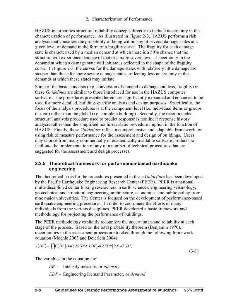
2.2.4 Earthquake Risk Analysis In 1997, FEMA and the National Institute for Building Sciences (NIBS, 1997) released the initial version of a computer software program (HAZUS) that comprised a regional seismic loss estimation model. The original version of HAZUS computed expected losses for large inventories of buildings using representative typical models intended to capture the average results of large inventories. A later version allows the input of building-specific data in the place of the default models (NIBS 2002). The calculation procedure for building losses is technically similar to that for first-generation performance based design procedures (Kircher 1997a,b). Rather than performance levels, the HAZUS algorithm is based on a series of damage states as illustrated in Figure 2-3
Figure 2-3: HAZUS damage states related to deformation of building
2. Characterization of Performance
2-8 Guidelines for Seismic Performance Assessment of Buildings 25% Draft
HAZUS incorporates structural reliability concepts directly to include uncertainty in the characterization of performance. As illustrated in Figure 2-3, HAZUS performs a risk analysis that considers the probability of being within any of several damage states at a given level of demand in the form of a fragility curve. The fragility for each damage state is characterized by a median demand at which there is a 50% chance that the structure will experience damage of that or a more severe level. Uncertainty in the demand at which a damage state will initiate is reflected in the shape of the fragility curve. In Figure 2-3, the curves for the damage states with relatively little damage are steeper than those for more severe damage states, reflecting less uncertainty in the demands at which these states may initiate.
Some of the basic concepts (e.g. conversion of demand to damage and loss, fragility) in these Guidelines are similar to those introduced for use in the HAZUS computer software. The procedures presented herein are significantly expanded and enhanced to be used for more detailed, building-specific analysis and design purposes. Specifically, the focus of the analysis procedures is at the component level (i.e. individual items or groups of item) rather than the global (i.e. complete building). Secondly, the recommended structural analysis procedure used to predict response is nonlinear response history analysis rather then the simplified nonlinear static procedure implicit in the function of HAZUS. Finally, these Guidelines reflect a comprehensive and adaptable framework for using risk to measure performance for the assessment and design of buildings. Users may choose from many commercially or academically available software products to facilitate the implementation of any of a number of technical procedures that are suggested for the assessment and design processes.
2.2.5 Theoretical framework for performance-based earthquake engineering
The theoretical basis for the procedures presented in these Guidelines has been developed by the Pacific Earthquake Engineering Research Center (PEER). PEER is a national, multi-disciplined center linking researchers in earth sciences, engineering seismology, geotechnical and structural engineering, architecture, economics, and public policy from nine major universities. The Center is focused on the development of performance-based earthquake engineering procedures. In order to coordinate the efforts of many individuals from the various disciplines, PEER developed a basic framework and methodology for projecting the performance of buildings.
The PEER methodology explicitly recognizes the uncertainties and reliability at each stage of the process. Based on the total probability theorem (Benjamin 1970), uncertainties in the assessment process are tracked through the following framework equation (Moehle 2003 and Deierlein 2004):
( ) ∫∫∫= )(IMdIMEDPdGEDPDMdGDMDVGDV λλ (3-1)
The variables in the equation are:
IM – Intensity measure, or intensity
EDP - Engineering Demand Parameter, or demand

2. Characterization of Performance
25% Draft Guidelines for Seismic Performance Assessment of Buildings 2-9
DM - Damage Measure, or damage state
DV - Decision variable, or projected loss
The equation is a formal expression of the performance assessment process. The last term on the right, λ(IM), is the probability of experiencing ground shaking of a given intensity, obtained from the basic hazard curve (see Sect.2.3.1). The relationship between intensity and the demand is the term EDP|IM (see Sect.2.3.2). Similarly the conversion of demand to damage is represented by DM|EDP (see Sect.2.3.3). Generating loss from damage is the term DV|DM (see Sect.2.3.3). The other operators in the equation represent the use of the total probability theorem allowing the uncertainties in the assessment process to be carried through the process. The term ( )λ DV represents the probability that the losses will be exceeded. The four procedural steps of performing this integration are illustrated in Figure 2-4.
Figure 2-4: Steps to generating a decision variable in the PEER methodology
(Moehle 2003)
2.3 Using Risk to Measure Performance Characterizing the performance of structures subject to earthquakes as the risk of incurring basic losses provides important improvements over first-generation performance evaluation and performance-based design procedures. In place of the conventional discrete performance levels and pass-fail approaches, performance assessment procedures presented in these Guidelines provide assessment of the anticipated consequences of earthquake shaking in terms of the response of individual components and the building as a whole (demands). These demands can be used to assess probable levels of damage. Once the likely damage is understood, it is possible to quantify the probable losses in terms of casualties, direct economic loss, and downtime. The incorporation of risk analysis techniques further enhances the results of the process with information about the confidence associated with assessments of such losses.
2.3.1 Intensity and Frequency of Occurrence of Earthquake Shaking The fact that a building is located close to one or more faults may make the possibility of losses due to earthquake an important consideration. The risk of incurring losses, however, is dependent on the strength (intensity) of shaking produced by these faults and how often (the frequency) such shaking will occur. Hazard analysis provides information
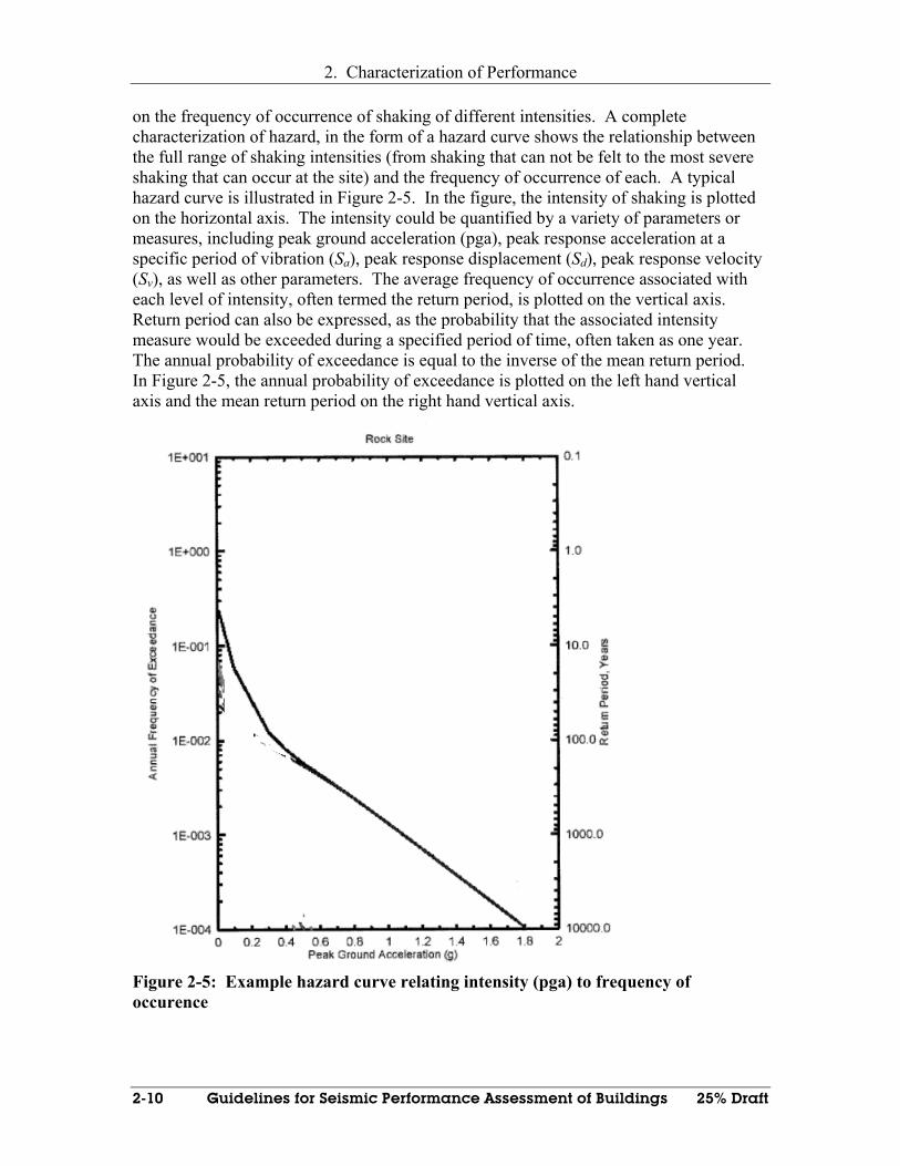
2. Characterization of Performance
2-10 Guidelines for Seismic Performance Assessment of Buildings 25% Draft
on the frequency of occurrence of shaking of different intensities. A complete characterization of hazard, in the form of a hazard curve shows the relationship between the full range of shaking intensities (from shaking that can not be felt to the most severe shaking that can occur at the site) and the frequency of occurrence of each. A typical hazard curve is illustrated in Figure 2-5. In the figure, the intensity of shaking is plotted on the horizontal axis. The intensity could be quantified by a variety of parameters or measures, including peak ground acceleration (pga), peak response acceleration at a specific period of vibration (Sa), peak response displacement (Sd), peak response velocity (Sv), as well as other parameters. The average frequency of occurrence associated with each level of intensity, often termed the return period, is plotted on the vertical axis. Return period can also be expressed, as the probability that the associated intensity measure would be exceeded during a specified period of time, often taken as one year. The annual probability of exceedance is equal to the inverse of the mean return period. In Figure 2-5, the annual probability of exceedance is plotted on the left hand vertical axis and the mean return period on the right hand vertical axis.
Figure 2-5: Example hazard curve relating intensity (pga) to frequency of occurence

2. Characterization of Performance
25% Draft Guidelines for Seismic Performance Assessment of Buildings 2-11
The hazard curve shown in Figure 2-5 indicates the probability of experiencing ground shaking of a given intensity at a site considering several potential faults that are located near the site, and also considering that earthquakes of different magnitude can occur on each of these faults. These types of hazard curves are typically produced by a probabilistic seismic hazard analysis, as discussed in Chapter 5. It is also possible to construct a hazard curve for a specific scenario earthquake, defined by a given earthquake magnitude and distance from the site. Such a hazard curve is shown in Figure 2-6. Like that in Figure 2-5, it relates intensity of shaking to probability of exceedance.
0.01
0.1
1
0.01 0.1 1 10
Spectral Response Accel. at 1 second Sa-1
Con
ditio
nal P
roba
bilit
y of
Exc
eedi
ng S
a for
a
Giv
en M
, R
Figure 2-6 Example scenario hazard curve relating intensity of spectral acceleration at 1-second to the probability of being exceeded for a given magnitude (M) and distance (R) from the site. Hazard curves, like those shown in Figure 2-5 and 2-6 can be used to generate ground motion parameters for use in an engineering analysis as part of a building performance assessment. In the procedures presented in this document, intensity is represented by smoothed elastic acceleration response spectra and suites of ground motions that are adjusted to these spectra.
2.3.2 Demand The next step in the process is to gauge the effects of the earthquake shaking of variable intensity on the building in engineering terms. These effects are measured by response quantities, or demands, obtained from structural analysis. Demands usually take the form of forces, accelerations and deformations, or other physical quantities that may be imposed by seismic shaking on the components of a building. In the procedures presented in this document, nonlinear response history analysis is used (see Figure 2-7). For each level of shaking intensity, a series of response history analyses are performed, using the ground motions that are adjusted to the spectrum that corresponds to the intensity level. Individual component demands, such as peak axial force in a brace and global demands, such as peak roof lateral displacement are recorded for each analysis.

2. Characterization of Performance
2-12 Guidelines for Seismic Performance Assessment of Buildings 25% Draft
Since the demands recorded from each analysis will typically be somewhat different, due to differences in the characteristics of the individual ground motion records, this process provides information on the uncertainty associated with estimating demands resulting from a given intensity of shaking. This is recorded in the form of an average demand for the given shaking intensity, and a measure of the variation in demand.
Structural model
Ground motionsGround motions
Component actions
δj
δi
θi
θj
Component actions
δj
δi
θi
θj
Component actions
δj
δi
θi
θj
Story drifts and forcesδij
Story drifts and forcesδij
Story drifts and forcesδij
Global displacement∆
Global displacement∆
Global displacement∆
Figure 2-7: Nonlinear response history analysis for suites of ground motions
scaled to a particular intensity provides statistical information on the relationship between demand and intensity.
2.3.3 Damage States Demand parameters obtained from structural analysis are important and meaningful to engineers in understanding the expected behavior of a building and its contents. However, they are not directly useful to decision makers for characterizing the consequences of extreme events in terms of the actual losses related to the damage that may occur. To get to these consequences, the demands must be converted to estimates of damage, in quantifiable terms. Damage states are used to relate the physical consequences of component and global demands to the safety implications and the need for repair or replacement. Section 2.2.4 illustrates how the concept of fragility is used in HAZUS to convert global demand (e.g. roof displacement) into the probability of being in any of several global different damage states (see Figure 2-3). In the procedures presented in this document the same basic concept is applied at both the component and global level using both global and component demands and fragilities (see Table 2-1 and 2-2). The results for any component, or group of components, are a relationship between demand and damage. By aggregating this information for all components for a given ground motion a total damage state for the building can be generated. Like the demands themselves, damage is treated statistically through the fragility relationships to reflect the uncertainty with this step in the process.

2. Characterization of Performance
25% Draft Guidelines for Seismic Performance Assessment of Buildings 2-13
Table 2-1: Representative component damage states for interior partitions
Slight- hairline cracking, requiring minor local patching and painting of walls
Moderate- cracking, requiring major patching, re-taping, and painting of walls
Extensive- replacement of some wallboard, general re-taping, patching, and painting
Severe- demolition and full replacement.
Table 2-2: Representative damage states for a steel column
Slight- forces less than 10% over elastic limits
Moderate- local buckling requiring in-situ repair
Extensive- major inelastic distortion requiring removal and replacement
Severe- collapse
2.3.4 Losses Once a total damage state is determined for a building, an estimate can be made of the losses associated with this damage. For direct economic losses, this can be visualized as the process that a contractor would go through to determine the cost to repair or replace damaged components and systems. The time to implement the repairs and bring the facility back into service can also be estimated to assess downtime. The total damage state also provides information on potential casualties.
In the procedures presented in this document, a statistical distribution of losses is generated for one or more shaking intensity levels by evaluating the damage and losses, from each of a number of different demand sets, that are statistically consistent with the shaking intensity.
2.3.5 Performance measures and stakeholder perspectives The resulting distribution of losses comprises a performance measure for the building in terms of three basic risk parameters:
• Casualties (Human loss and serious injuries).
• Direct economic loss (cost to repair or replace).
• Downtime (Occupancy loss).
These measures of performance can be generated for several different types of performance assessments depending on the specific decision making needs of the stakeholders:
• a.) Minimum performance standards (prescriptive code compliance)
The basic risk parameters derived from the performance assessment methodology can either be used to demonstrate that a design meets the performance criteria intended by the code, or alternatively, can be used to improve the statements of
2. Characterization of Performance
2-14 Guidelines for Seismic Performance Assessment of Buildings 25% Draft
performance criteria currently underlying the codes. For example, the primary purpose of seismic provisions in present prescriptive codes is to provide for a minimum level of public safety. However, absolute protection is not possible and current code criteria make no attempt to quantity the actual risk. The casualties risk parameter that results from the performance assessment methodology provides a quantifiable measure of safety for a building design. With this tool in place, codes could specify a maximum allowable life safety risk. This could be expressed in several forms, for example not greater than a 10% chance of single life loss, given a 475-year event, or alternatively, less than a 0.0002 chance per year of single life loss. Similarly, codes could require maximum levels of risk associated with direct economic losses or downtime depending on the importance or function of a facility (e.g. public buildings, hospitals).
b.) Conventional performance objectives
Similar to the code application described above, the qualitative performance levels of current performance-based design procedures (e.g. FEMA 356) could be indexed easily to the quantifiable risk parameters obtained from the performance assessment methodology. For example, Immediate Occupancy could be defined as a 90% confidence of less than a day’s occupancy loss for shaking with a 475 year mean return period.
c.) Financially based decisions
The use of the risk-based performance characterization enables the engineer, facility owner, building tenant, city planner, and others, to answer important questions in economic terms. For example:
Should the owner retrofit a facility to reduce losses from potential earthquakes?
The engineer formulates the basic risk parameters in dollars for the existing facility for shaking of all intensities. The risk is expressed as average losses to be expected each year (i.e. dollars per year) for the life of the building in its current condition. The engineer then conceptually develops a retrofit design to address the facility’s seismic deficiencies and assesses the basic risk parameters for the improved facility. The amortized cost of retrofit should be less than the reduction in average expected annual losses, or the retrofit would not make economic sense. An optimal level of retrofit could be determined by repeating this exercise until a maximum cost/benefit ratio is obtained.
For a new facility, is it preferable to use shear walls or unbonded braces as the lateral-force-resisting system?
The engineer performs a conceptual design and cost estimate for both options, and then determines the net present value of the basic risk parameters for each option for the extreme events of interest. If the cost premium for the more expensive alternative is less than benefit in terms of reduced expected losses, the additional cost is economically justified.
What are the Probable Maximum Losses expected for a building?
2. Characterization of Performance
25% Draft Guidelines for Seismic Performance Assessment of Buildings 2-15
Some lenders require that the losses associated with a specific level of shaking (e.g. 10% chance of being exceeded in 50 yrs) be less than a given percentage (e.g. 20%) of the replacement cost for the building. In this case, the engineer can determine the expected losses directly for the given intensity level and compare this projected loss with the replacement cost. Current procedures for this process are very approximate and rely heavily on the opinion of the individual engineer. The guidelines in this document will result in a greatly refined estimate and less variation attributable to personal opinion.
Should an owner invest in a design for higher performance, accept the risk, or transfer the risk through purchase of insurance?
An economic analysis can identify the optimal investment in risk reduction through improved performance. Beyond some level the incremental return on investment drops. An owner may choose to supplement the design with risk transfer through insurance or simply accept it. By understanding the excess risk and the probabilistic distribution of that risk over a range of hazard levels, the owner is in a better position to determine a risk management approach that makes most economic sense for him or her.
d.) Specialized decision needs
Individual stakeholders often relate to particular information on the risk implications of design decisions that are most useful to their decision processes. Often these relate to specific earthquake scenarios. The basic risk parameters can be easily re-formatted to provide such information. For example, they can address questions such as:
• What is the chance of a death or serious injury in my building due to an M7 earthquake on a specific fault in the next 20 years?
• Can I be 90% sure that a M6.5 earthquake will not put me out of business with a direct economic loss of over a million dollars in the next 50 years?
In these cases the basic risk parameters are assessed for specific scenario event.
Specialized decision needs can also be based on assessments that consider all potential scenarios as well:
• Is there greater than a 10% chance that our hospital will be unable to accept new patients for more than a week after an earthquake in the next 50 years?
• Is there greater than a 10% chance that all fire stations in a city will be unable to service the fire department following an earthquake?
• What is the chance that the repair cost for my building would exceed $2 million in the event of an earthquake?
In summary, the performance assessment process presented in this document enables the engineer to provide decision-makers with important information that is not currently attainable, except by judgmental and qualitative means.

2. Characterization of Performance
2-16 Guidelines for Seismic Performance Assessment of Buildings 25% Draft
2.4 References
ASCE, 2000, Prestandard and Commentary for the Seismic Rehabilitation of Buildings, FEMA 356 Report, prepared by the American Society of Civil Engineers; published by the Federal Emergency Management Agency, Washington, DC, www.fema.gov.
ATC, 1996, Seismic Evaluation and Retrofit of Concrete Buildings, Volumes 1 and 2, ATC-40 Report, Applied Technology Council, Redwood City, California, www.atcouncil.org.
Benjamin, J.R., and Cornell, C.A., Probability, statistics, and decision for civil engineers, New York, McGraw-Hill (1970).
Deierlein, G.G., and Hamilton, S., Framework for structural fire engineering and design methods, NIST-SFPE Workshop for Development of a National R&D Roadmap for Structural Fire Safety Design and Retrofit of Structures: Proceedings, 2004.
Federal Emergency Management Agency (FEMA), 2000, NEHRP Recommended Provisions for Seismic Regulations for New Buildings and Other Structures, FEMA 368 Report, Federal Emergency Management Agency, Washington, D.C.
ICC, International Performance Code, 2003, International Code Council, Country Club Hills, IL
Kircher, Charles A., Aladdin A. Nassar, Onder Kustu and William T. Holmes, 1997a. “Development of Building Damage Functions for Earthquake Loss Estimation,” Earthquake Spectra, Vol. 13, No. 4, Earthquake Engineering Research Institute, Oakland, CA, www.eeri.org.
Kircher, Charles A., Robert K. Reitherman, Robert V. Whitman and Christopher Arnold, 1997b. “Estimation of Earthquake Losses to Buildings,” Earthquake Spectra, Vol. 13, No. 4, Earthquake Engineering Research Institute, Oakland, CA, www.eeri.org.
Moehle, J. P., “A Framework for Performance-Based Earthquake Engineering,” Proceedings, Tenth U.S.-Japan Workshop on Improvement of Building Seismic Design and Construction Practices, 2003, ATC-15-9 Report, Applied Technology Council, Redwood City, CA.
National Institute of Building Science (NIBS), 1997. HAZUS99 Technical Manual. Developed by the Federal Emergency Management Agency through agreements with the National Institute of Building Sciences, Washington, D.C., www.nibs.org or www.fema.gov.
National Institute of Building Science (NIBS), 2002. HAZUS99 Advanced Engineering Building Module Technical and User’s Manual. Developed by the Federal Emergency Management Agency through agreements with the National Institute of Building Sciences, Washington, D.C., www.nibs.org or www.fema.gov.

25% Draft Guidelines for Seismic Performance Assessment of Buildings 3-1
3 Framework for Performance Assessment
3.1 Introduction This section presents a basic framework for building earthquake performance assessment. The purpose of the assessment is to provide information for design decisions by engineers and other stakeholders, either for a new building or the evaluation and retrofit of an existing building.
Within the basic framework, a number of alternative procedures can be used to define the hazard, predict the response, determine damage, and calculate performance in terms of probable casualties, direct economic loss and downtime. These Guidelines present one set of such procedures. An example application of the assessment procedures outlined in this chapter illustrates the process in accompanying figures. Details on application of the procedures contained herein are presented in the following chapters, as referenced in this Chapter.
A calculation tool is provided on a CD-ROM with these Guidelines, to assist in performing some of the mathematics associated with assessing building performance.
Reader Note: It is envisaged that the “calculation tool” will be either a spreadsheet or Mathcad type application that will facilitate the calculation of performance. Input to the calculation tool will include information on building composition and values, the criticality of various systems and components on building occupancy and casualties, information on the damageability fo these systems and components and information obtained from structural analysis. Based on this input data, the calculation tool will provide various measures of performance including assessments of probable direct economic losses, downtime and casualties, at various probabilities of exceedance. This calculation tool is not presently developed, but will be provided with later drafts of the Guidelines.
3.2 Levels of Assessment Two alternative levels of assessment are possible under these Guidelines:
Conceptual Assessment
Detailed Assessment
The basic steps of performing either type of assessment are the same. The primary difference between the levels of assessment is that for conceptual level assessments, it is assumed that only summary level information is available on the building’s construction occupancy while for detailed level assessments, precise data on the building’s design and construction is available. Accordingly, in conceptual level assessments, there is greater reliance on generalized data on building inventory and construction, based on building age, structural system type and building use, while for detailed assessments, building-specific data for each of these is required. Further, for conceptual assessments,
3. Framework for Performance Assessment
3-2 Guidelines for Seismic Performance Assessment of Buildings 25% Draft
recognizing the imprecise nature of building definition, relatively simple methods of structural analysis are relied upon to predict building response.
3.3 Types of Assessment These Guidelines may be used to perform three different types of assessment:
Intensity-based assessment
Scenario-based assessment
Time-based assessment
These various types of assessments are described in the sections that follow.
3.3.1 Intensity-based assessments An intensity-based performance assessment is an estimate of the probable losses, given that the building experiences a specific intensity of shaking. In these Guidelines, intensity is represented by a 5% damped, elastic acceleration response spectrum. Selected ground motions are adjusted to match the specified intensity. This type of assessment answers questions such as:
• What are the chances of losses of given amount, if the building is subjected to ground motion of specific intensity? For example, what are the chances of experiencing direct economic losses greater than $1M for ground motions that produce a smoothed spectrum with a peak ground acceleration of 0.5g at the site?
• What are the expected number of days of occupancy interruption if the building is subjected to ground shaking matching the code design spectrum?
• What is the risk of incurring casualties, if the building is affected by a maximum considered earthquake?
Note that the intensity of motion may, or may not, be probabilistically qualified. That is, the amplitude of the spectrum can be specified as having a specific value, as in the above example, or the amplitude could be expressed as having a particular probability of being exceeded (e.g. 10% chance of being exceeded in 50 years).
Figure 3-1 illustrates the important steps in the procedure for performing an intensity-based assessment. These steps are discussed in detail in later sections of this Chapter.
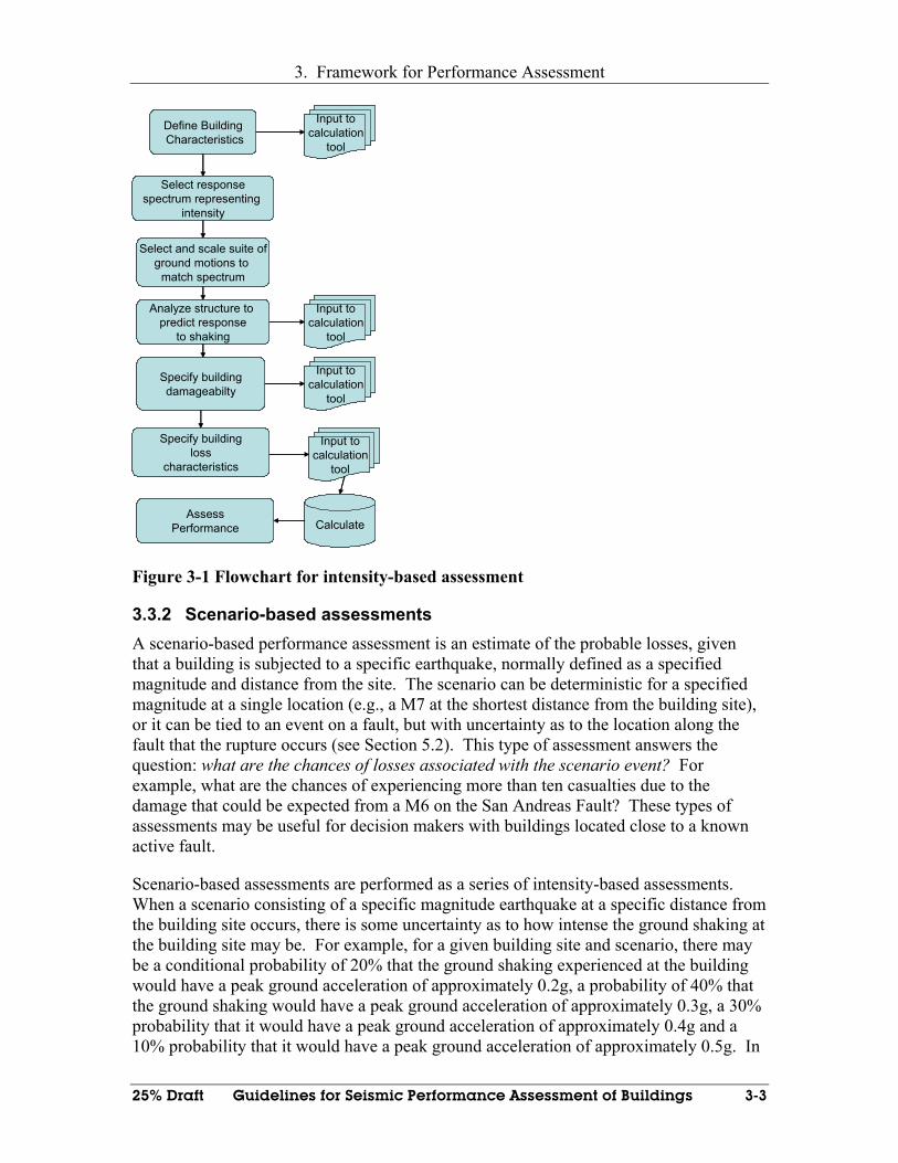
3. Framework for Performance Assessment
25% Draft Guidelines for Seismic Performance Assessment of Buildings 3-3
Define BuildingCharacteristics
Select responsespectrum representing
intensity
Select and scale suite ofground motions to
match spectrum
Input tocalculation
tool
Analyze structure to predict response
to shaking
Input tocalculation
tool
Specify buildingdamageabilty
Input tocalculation
tool
Specify buildingloss
characteristics
Input tocalculation
tool
AssessPerformance Calculate
Figure 3-1 Flowchart for intensity-based assessment
3.3.2 Scenario-based assessments A scenario-based performance assessment is an estimate of the probable losses, given that a building is subjected to a specific earthquake, normally defined as a specified magnitude and distance from the site. The scenario can be deterministic for a specified magnitude at a single location (e.g., a M7 at the shortest distance from the building site), or it can be tied to an event on a fault, but with uncertainty as to the location along the fault that the rupture occurs (see Section 5.2). This type of assessment answers the question: what are the chances of losses associated with the scenario event? For example, what are the chances of experiencing more than ten casualties due to the damage that could be expected from a M6 on the San Andreas Fault? These types of assessments may be useful for decision makers with buildings located close to a known active fault.
Scenario-based assessments are performed as a series of intensity-based assessments. When a scenario consisting of a specific magnitude earthquake at a specific distance from the building site occurs, there is some uncertainty as to how intense the ground shaking at the building site may be. For example, for a given building site and scenario, there may be a conditional probability of 20% that the ground shaking experienced at the building would have a peak ground acceleration of approximately 0.2g, a probability of 40% that the ground shaking would have a peak ground acceleration of approximately 0.3g, a 30% probability that it would have a peak ground acceleration of approximately 0.4g and a 10% probability that it would have a peak ground acceleration of approximately 0.5g. In

3. Framework for Performance Assessment
3-4 Guidelines for Seismic Performance Assessment of Buildings 25% Draft
order to assess the performance of the building for this scenario, a separate intensity-based performance assessment is performed, using the procedures illustrated in Figure 3-1, at each of these intensity levels (i.e., 0,1g, 0.2g, 0,3g, 0.4g, and 0.5g). The total probable losses, given the occurrence of the scenario is computed as the sum of the losses predicted at each intensity level, factored by the conditional probability that intensity level will be experienced. Section 5.2.3 of these Guidelines provides information on how to determine the probabilities of different intensities of ground shaking for an earthquake scenario.
3.3.3 Time-based assessments A time-based assessment is an estimate of the probable consequences, considering all potential earthquakes that may occur in a given period of time, and the probability of each. The time-based type of assessment answers the question: what are the chances of losses exceeding a given amount, over a given time period? For example, what are the chances of experiencing downtime longer than 30 days over a fifty-year life of a building?
Time-based assessments are also performed as a series of intensity-based assessments. To do this, a probabilistic seismic hazard analysis must be performed to indicate the probability of exceedance of various intensities of ground shaking within the time period of interest (e.g. 50 years), ranging from intensities that would barely be felt to the maximum intensity ever likely to be experienced at the site. From this probabilistic seismic hazard data, a series of ground shaking intensities (e.g. pga=0.1g, pga=0.2g, …. pga=0.8g) would be selected and the probability of occurrence of each in the time period determined. Then, an intensity based performance assessment of the building is conducted at each of these intensity levels. The probable loss in the period of time of interest, in casualties, direct economic loss, or downtime, is calculated as the sum of these losses at each intensity level, factored by the probability of occurrence of each intensity level in the period of time. Section 5.2.4 provides information on probabilistic seismic hazard analysis and selection of appropriate intensities and their probability of occurrence for time-based assessment.
Reader Note: At this time (November 2005) detailed procedures have only been developed for assessment of direct economic loss. Detailed procedures for assessment of life safety and downtime risks are not fully developed. It is anticipated, however, that the assessment of these losses can be accomplished with modifications to the basic procedures presented for direct economic loss, which will be presented in later editions of these Guidelines.
3.4 General Assessment Procedure
The section presents in some detail, the basic steps required to conduct a performance assessment. Detailed guidelines are provided in later chapters, as referenced herein.

3. Framework for Performance Assessment
25% Draft Guidelines for Seismic Performance Assessment of Buildings 3-5
3.4.1 Building Definition
The first step in performance assessment is to define the building that is being assessed. This includes definition of the location of the building, the characteristics of the site, the size of the building, use, structural systems, types and locations of architectural, mechanical, electrical and plumbing systems that are present, type and nature of tenant contents, and the value of each of these building constituent parts.
The level of definition of the building required is dependent on the level of assessment performed. For conceptual level assessments, the following minimum level of information is needed: building site location and site class, building size, general use, the type of structural system used, and the natural period and yield strength of the lateral force resisting system. From this general descriptive data, the calculation tool provided with these Guidelines can apply default building data on the likely distribution and quantities of various nonstructural components and systems, and their values. For detailed level assessments, specific inventory and value data must be supplied.
Figure 3-2 is illustrative of the level of data required to define a building for conceptual level assessments. Based on this level of definition, default inventories of nonstructural systems can be assigned from the databases contained in these Guidelines and the companion calculation tool.
Year of Const. 2000
Design Code; 1997 UBC
Height: 3 stories; 14 ft. floor to floor; 42 ft total above grade; no basement
Area: 22,736 sq.ft. per floor; 68,208 sq.ft. total
Occupancy: General office space
Location: Berkeley, California
Site Class: C
Period T: 0.5 seconds
Yield Strength: 0.3W
Figure 3-2 Example conceptual level building definition

3. Framework for Performance Assessment
3-6 Guidelines for Seismic Performance Assessment of Buildings 25% Draft
Outline specification Note: Components included in performance
groups used to monitor damage in the model are shaded.
1. Foundations:
spread footings and grade beams 2. Lateral Resisting System: (see Figs.)
steel moment frames (actual building is eccentrically braced frames)
3. Vertical Support System: light weight reinforced concrete metal deck steel beams and columns
4. Exterior Cladding: precast concrete wall panels with aluminum frame windows plaster finish over metal stud wall framing, furring and insulation storefront aluminum windows and exterior doors
5. Roofing & Waterproofing: conventional built-up roofing, flashing, and drainage
6. Interior Partitions, Doors & Glazing: gypsum wallboard on metal studs hollow core wood and metal doors conventional glazing
7. Floor, Wall & Ceiling Finishes: suspended drop in ceilings floor finishes sandstone tile flooring carpet ceramic tiles sealed concrete base vinyl sandstone rubber wall finishes ceramic tiles paint gypsum board
8. Equipment & Specialties toilet partitions (floor mounted) handicapped regular bathroom accessories mirrors casework bathroom vanity shelf miscellaneous equipment building directory code required signage exterior signage (door ID)
entry mats window blinds lockers, metal fire extinguisher cabinets corner guards marker boards / tackboards mail boxes / postal specialties telephone booths
9. Stairs & Vertical Transportation: metal stairs with concrete filled treads traction elevators
10. Plumbing Systems: sanitary fixtures w/ rough in and connection piping sanitary waste, vent and service piping water treatment, storage and circulation surface water drainage gas distribution condensate drains testing and sterilization
11. Heating, Ventilating & Air Conditioning:
heat generation and chilling steam heat exchanger air conditioning units, packaged type, roof mounted circulation pumps and specialties piping, fittings, valves and insulation air separator expansion tank chemical feeder cold water makeup air distribution and return testing and balancing controls and instrumentation
12. Electric Lighting, Power & Communications main power and distribution including UPS machine and equipment power lighting Lighting and power specialties telephone and communication systems alarm and security systems
13. Fire Protection Systems fire sprinkler system (wet system) standpipes and hose valves
Figure 3-3 Representative Data Input for Detailed Level Assessments
3. Framework for Performance Assessment
25% Draft Guidelines for Seismic Performance Assessment of Buildings 3-7
Figure 3-3 is representative of the level of data required for detailed level assessments. Although information on the value of all building components is necessary, in order to permit estimates of repair costs to be formed, it is recognized that not all building components are subject to earthquake damage. Some components, for example, toilet fixtures, are inherently rugged and are not damaged by earthquakes. Those components that are subject to damage are grouped together into sets that have similar damage and consequence characteristics, termed performance groups. For example, ceiling systems, fire sprinkler distribution piping and lighting fixtures at a story level may all be placed in a common performance group, because all are subject to damage from building acceleration at the same level of the structure and damage to these components would effect use of the space at this story level. In Figure 3-3, components that are assigned to performance groups are highlighted by shading, to illustrate this concept.
Chapter 4 of these Guidelines provides more specific and detailed on guidance on how buildings are defined and performance groups assembled. Section 3.7 below also provides information on the performance group concept.
3.5 Hazard analysis Detailed provisions for hazard assessment are the subject of Chapter 5.
3.5.1 Intensity-based For intensity-based assessments, a response spectrum, representing the intensity for which the performance is to be assessed, and a suite of ground motions, scaled to this spectrum are required. Scaling must be performed in an appropriate manner to capture the natural uncertainty associated with ground motion of a particular intensity. Figure 3-4 illustrates the scaling of ground motions to match a target spectrum. Refer to Section 5.3 for information on developing spectra. Refer to Section 5.6 for detailed information on selecting and scaling ground motions.
Reader Note: Much controversy currently prevails in the industry as to appropriate methods for scaling ground motions to match a target spectrum. Methods commonly employed today include: amplitude scaling to envelope the spectrum over a range of periods; spectral matching in the time domain and spectral matching in the frequency domain; amplitude scaling to match the target at a specific period; amplitude scaling to minimize the error between the spectrum for the recorded ground motion and the target, over a range of periods. Each of these methods has advantages and disadvantages. Figure 3-4 illustrates the method in which records are scaled to match the target spectrum at the fundamental period of the building. Chapter 5 suggests using a least squares approach to error minimization over a range of periods. Work is currently underway at PEER, BSSC, COSMOS and other organizations to develop a consensus on appropriate methods of scaling. Later versions of these Guidelines will take advantage of this ongoing work.
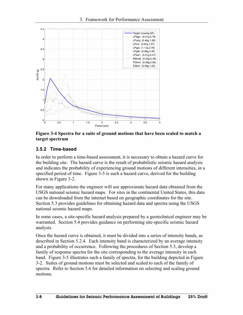
3. Framework for Performance Assessment
3-8 Guidelines for Seismic Performance Assessment of Buildings 25% Draft
0 0.5 1 1.5 2 2.5 3 3.5 40
0.5
1
1.5
2
2.5
3
3.5
4
4.5
Period (sec)
Sa-
FN
(g)
Target (maxAg,SF)LPlgpc (0.51g,0.79)
LPsrtg (0.46g,1.28)
LPcor (0.81g,1.67)
LPgav (1.11g,3.79)LPgilb (0.66g,2.35)
LPlex1 (0.21g,0.47)
KBkobj (0.42g,0.49)
TOhino (0.59g,0.56)EZerzi (0.59g,1.23)
Figure 3-4 Spectra for a suite of ground motions that have been scaled to match a target spectrum
3.5.2 Time-based In order to perform a time-based assessment, it is necessary to obtain a hazard curve for the building site. The hazard curve is the result of probabilistic seismic hazard analysis and indicates the probability of experiencing ground motions of different intensities, in a specified period of time. Figure 3-5 is such a hazard curve, derived for the building shown in Figure 3-2.
For many applications the engineer will use approximate hazard data obtained from the USGS national seismic hazard maps. For sites in the continental United States, this data can be downloaded from the internet based on geographic coordinates for the site. Section 5.3 provides guidelines for obtaining hazard data and spectra using the USGS national seismic hazard maps.
In some cases, a site-specific hazard analysis prepared by a geotechnical engineer may be warranted. Section 5.4 provides guidance on performing site-specific seismic hazard analysis.
Once the hazard curve is obtained, it must be divided into a series of intensity bands, as described in Section 5.2.4. Each intensity band is characterized by an average intensity and a probability of occurrence. Following the procedures of Section 5.3, develop a family of response spectra for the site corresponding to the average intensity in each band. Figure 3-5 illustrates such a family of spectra, for the building depicted in Figure 3-2. Suites of ground motions must be selected and scaled to each of the family of spectra. Refer to Section 5.6 for detailed information on selecting and scaling ground motions.

3. Framework for Performance Assessment
25% Draft Guidelines for Seismic Performance Assessment of Buildings 3-9
Figure 3-5 Hazard curve for building illustrated in Figure 3-2
Figure 3-6 Family of spectra, representing different intensities of motion at a site
3.5.3 Scenario-based The same type of hazard information required for a time-based assessment is also required for a scenario-based assessment. The primary difference is that rather than
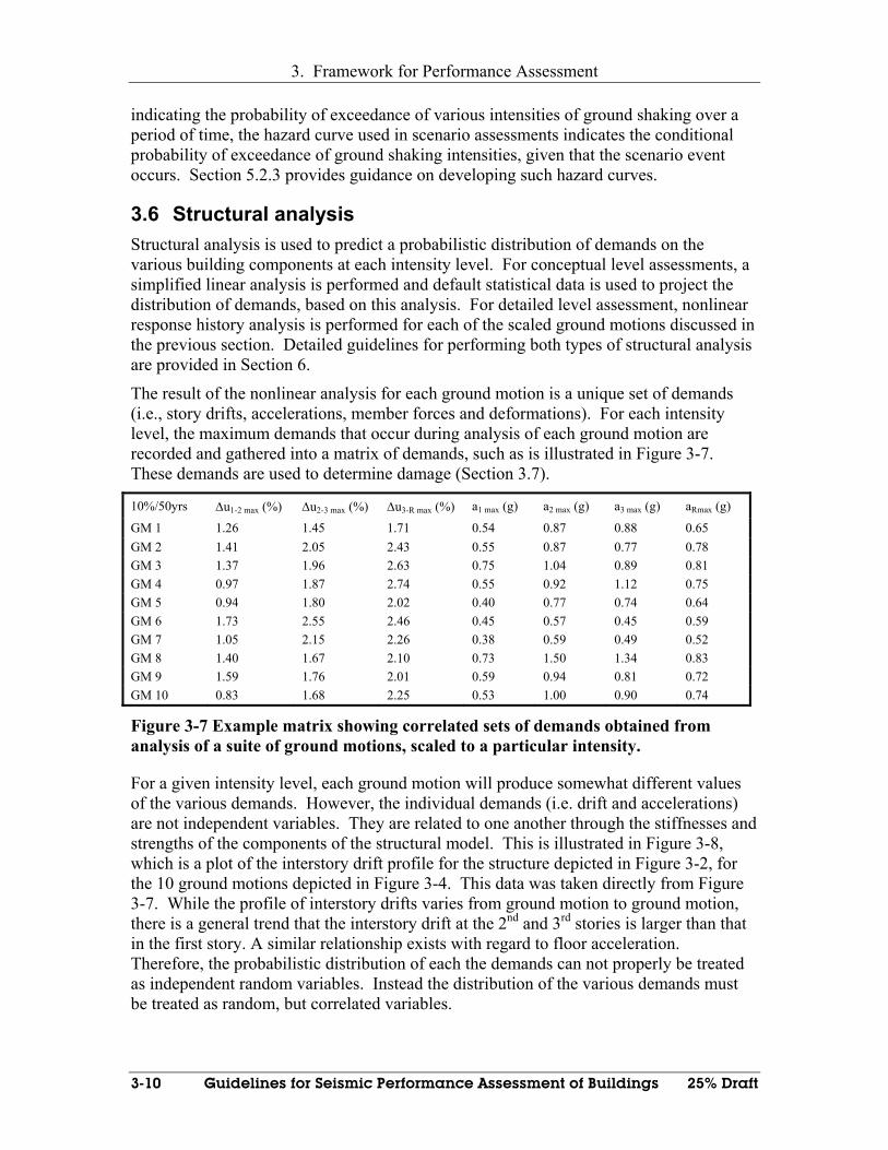
3. Framework for Performance Assessment
3-10 Guidelines for Seismic Performance Assessment of Buildings 25% Draft
indicating the probability of exceedance of various intensities of ground shaking over a period of time, the hazard curve used in scenario assessments indicates the conditional probability of exceedance of ground shaking intensities, given that the scenario event occurs. Section 5.2.3 provides guidance on developing such hazard curves.
3.6 Structural analysis Structural analysis is used to predict a probabilistic distribution of demands on the various building components at each intensity level. For conceptual level assessments, a simplified linear analysis is performed and default statistical data is used to project the distribution of demands, based on this analysis. For detailed level assessment, nonlinear response history analysis is performed for each of the scaled ground motions discussed in the previous section. Detailed guidelines for performing both types of structural analysis are provided in Section 6.
The result of the nonlinear analysis for each ground motion is a unique set of demands (i.e., story drifts, accelerations, member forces and deformations). For each intensity level, the maximum demands that occur during analysis of each ground motion are recorded and gathered into a matrix of demands, such as is illustrated in Figure 3-7. These demands are used to determine damage (Section 3.7).
10%/50yrs ∆u1-2 max (%) ∆u2-3 max (%) ∆u3-R max (%) a1 max (g) a2 max (g) a3 max (g) aRmax (g)
GM 1 1.26 1.45 1.71 0.54 0.87 0.88 0.65 GM 2 1.41 2.05 2.43 0.55 0.87 0.77 0.78 GM 3 1.37 1.96 2.63 0.75 1.04 0.89 0.81 GM 4 0.97 1.87 2.74 0.55 0.92 1.12 0.75 GM 5 0.94 1.80 2.02 0.40 0.77 0.74 0.64 GM 6 1.73 2.55 2.46 0.45 0.57 0.45 0.59 GM 7 1.05 2.15 2.26 0.38 0.59 0.49 0.52 GM 8 1.40 1.67 2.10 0.73 1.50 1.34 0.83 GM 9 1.59 1.76 2.01 0.59 0.94 0.81 0.72 GM 10 0.83 1.68 2.25 0.53 1.00 0.90 0.74
Figure 3-7 Example matrix showing correlated sets of demands obtained from analysis of a suite of ground motions, scaled to a particular intensity.
For a given intensity level, each ground motion will produce somewhat different values of the various demands. However, the individual demands (i.e. drift and accelerations) are not independent variables. They are related to one another through the stiffnesses and strengths of the components of the structural model. This is illustrated in Figure 3-8, which is a plot of the interstory drift profile for the structure depicted in Figure 3-2, for the 10 ground motions depicted in Figure 3-4. This data was taken directly from Figure 3-7. While the profile of interstory drifts varies from ground motion to ground motion, there is a general trend that the interstory drift at the 2nd and 3rd stories is larger than that in the first story. A similar relationship exists with regard to floor acceleration. Therefore, the probabilistic distribution of each the demands can not properly be treated as independent random variables. Instead the distribution of the various demands must be treated as random, but correlated variables.
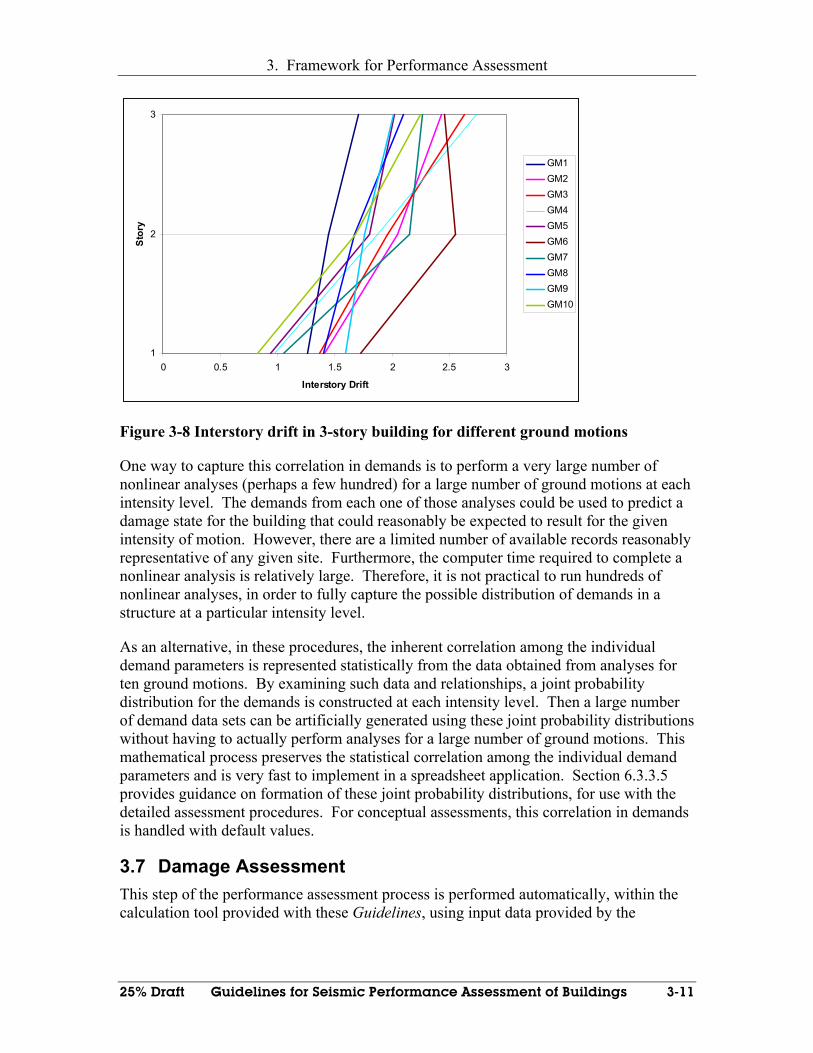
3. Framework for Performance Assessment
25% Draft Guidelines for Seismic Performance Assessment of Buildings 3-11
1
2
3
0 0.5 1 1.5 2 2.5 3
Interstory Drift
Stor
y
GM1GM2GM3GM4GM5GM6GM7GM8GM9GM10
Figure 3-8 Interstory drift in 3-story building for different ground motions
One way to capture this correlation in demands is to perform a very large number of nonlinear analyses (perhaps a few hundred) for a large number of ground motions at each intensity level. The demands from each one of those analyses could be used to predict a damage state for the building that could reasonably be expected to result for the given intensity of motion. However, there are a limited number of available records reasonably representative of any given site. Furthermore, the computer time required to complete a nonlinear analysis is relatively large. Therefore, it is not practical to run hundreds of nonlinear analyses, in order to fully capture the possible distribution of demands in a structure at a particular intensity level.
As an alternative, in these procedures, the inherent correlation among the individual demand parameters is represented statistically from the data obtained from analyses for ten ground motions. By examining such data and relationships, a joint probability distribution for the demands is constructed at each intensity level. Then a large number of demand data sets can be artificially generated using these joint probability distributions without having to actually perform analyses for a large number of ground motions. This mathematical process preserves the statistical correlation among the individual demand parameters and is very fast to implement in a spreadsheet application. Section 6.3.3.5 provides guidance on formation of these joint probability distributions, for use with the detailed assessment procedures. For conceptual assessments, this correlation in demands is handled with default values.
3.7 Damage Assessment This step of the performance assessment process is performed automatically, within the calculation tool provided with these Guidelines, using input data provided by the
3. Framework for Performance Assessment
3-12 Guidelines for Seismic Performance Assessment of Buildings 25% Draft
engineer. This section describes the processes used by the calculation tool and the information that the engineer must supply to support the calculation.
In order to capture the potential variability in damage at a given intensity of ground shaking, damage is assessed for each of a series of realizations. Each realization represents one possible set of demands that the structure could experience for the given intensity of shaking. In these procedures, a minimum of 200 realizations are generated for each intensity level, using the joint probability distribution discussed in the previous section. This provides a reasonable distribution of potential demand for each intensity level, representative of the inherent variability in the ground motion.
Each set of demands generated from the structural analysis are used to determine one possible distribution of damage in the building for the given intensity level. Rather than assessing the damage to each individual component, the components are grouped together into sets that have similar susceptibility to damage and similar consequences of damage. These sets of components are termed performance groups.
Damage states are used to define the severity of damage experienced by the set of components in a particular performance group. For assessments of direct economic loss and downtime, damage states are defined in terms of the repair actions that would be required to correct the damaged components to a state equivalent to that which existed prior to the shaking event and the resulting demands. For assessment of casualties, damage states are defined in terms of conditions that pose a risk to life. Fragility relationships are used to define the probability of the components within a performance group being in each damage state as a function of a demand parameter, for example, interstory drift. Chapter 7 contains detailed information on structural damage states and fragilities. Chapter 8 provides corresponding data for nonstructural components and systems. A total damage state representative of the repairs required for the entire building (or condition of threat to life safety) is generated from the individual performance group damage states for each set of demands. For direct economic losses, the total damage state is essentially a bill of repairs that would be required to return the building to its previous condition. Losses are determined using consequence functions that account for the correlation of various aspects of the damage. For example, the unit costs associated with various repairs depend on the total quantities for the entire building as opposed to those ascribed to individual components.
3.7.1 Performance groups It is neither practical nor desirable to model each and every component of a building separately to assess its performance. This section describes the use of performance groups (collections of components and systems) to monitor the damage sustained by the building for a particular earthquake realization. In general, performance groups are developed to address specific needs of an assessment. In many instances, however, the performance groups are similar. Suggested performance groups for buildings of typical use and construction are presented in Chapter 4. Generally, performance groups include components that will experience the same, or very similar demands, will be damaged by the same type of demand (e.g. interstory drift), will have similar damage states, and have similar fragilities. Figure 3-9 illustrates the performance groups used to assess the

3. Framework for Performance Assessment
25% Draft Guidelines for Seismic Performance Assessment of Buildings 3-13
performance of the building illustrated in Figure 3-1. Appendix B provides specific guidance on forming performance groups. Name Location EDP Components Damage states (other than zero) Notes
SH12 between levels 1 and 2 d 1-2
SH23 between levels 2 and 3 d 2-3
SH3R between levels 3 and R d 3-R
EXTD12 between levels 1 and 2 d 1-2
EXTD23 between levels 2 and 3 d 2-3
EXTD3R between levels 3 and R d 3-R
INTD12 between levels 1 and 2 d 1-2
INTD23 between levels 2 and 3 d 1-2
INTD3R between levels 3 and R d 3-R
INTA2 below level 2 a 1
INTA3 below level 3 a 2
INTAR below level R a 3
CONT1 at level 1 a 1 3
CONT2 at level 2 a 2 3
CONT3 at level 3 a 3 2
EQUIPR at level R a R Equipment on roof 2
Fragilities the same for all; quantities and repairs similar
Same fragilitles
Same fragilitles
Same fragilitlesInterior nonstructural acceleration sensitive: ceilings, lights, sprinkler heads, etc
Contents: General office on first and second floor, computer center on third
Structural lateral: lateral load resisting system; damage oriented fragility (direct loss calculations)
Exterior enclosure: panels, glass, etc.
Interior nonstructural drift sensitive: partitions, doors, glazing,etc
3 each
2 each
2 each
3 each
Figure 3-9 Performance groups used to assess example building
3.7.2 Performance group damage states and fragilities For each performance group, two or more damage states must be defined. There is always the potential for a “no damage state” and a “complete” damage state. For many performance groups, damage characterization can be further refined with intermediate damage states 1DS to −1jDS that represent levels of damage between “none” and “complete”. The probability that the components in s a performance group will be damaged to a given or more severe state of damage is obtained from a probability distribution, termed a fragility function. Fragility functions are generally represented by a lognormal distribution having a median value defined by iDSD and a dispersion β
iDS (i.e.standard deviation of the natural logarithm of the initiating demand for the damage state). Note that uncertainty β
iDS represents the uncertainty associated solely with the damage and is independent of uncertainty with respect to shaking intensity and demand. It primarily reflects variability in construction and material quality, as well as the extent that the occurrence of damage is totally dependent on the single demand parameter and the relative amount of knowledge that affects component fragility estimates. Figure 3-10 presents a typical fragility function. In the figure, EDP represents the demand, for example interstory drift or floor acceleration, that is used to predict the onset of various levels of damage, which are indicated by the damage states, DS1, DS2, etc. The probability, at a given demand, that the components in a performance group will be damaged to, but not beyond a given damage state, Di, is given by reading vertically in the fragility curve from the value of the demand and subtracting the probability of exceeding damage state, Di+1 from the probability of exceeding damage state Di.

3. Framework for Performance Assessment
3-14 Guidelines for Seismic Performance Assessment of Buildings 25% Draft
None
CompleteDS1 DS2 DS3 DSj
0
0.5
1.0
( )P iDS DS≥
EDP1EDP 2EDP 3EDP jEDP
None
CompleteDS1DS1 DS2DS2 DS3DS3 DSjDSj
0
0.5
1.0
( )P iDS DS≥
EDP1EDP 2EDP 3EDP jEDP
Figure 3-10: Performance group damage states and fragilities The damage states are defined in terms of either the degree or scope of repair (for direct economic losses and downtime) or percentage of building collapse (for casualty computations). For direct economic loss assessment, a list of required repairs, should the damage state occur, is prepared. This list of repairs, or bill of repairs, depends on the actual physical material quantities comprising all of the components in the group. The repairs that represent the damage states are specific quantities of material and labor required to return the entire group to a pre-event condition. Figure 3-11 illustrates this concept by indicating the description of damage states for performance group SH12 for the example building depicted in Figure 3-2. Figure 3-12 shows fragility curves associated with the damage states indicated in Figure 3-11.
Performance Group SH12
DS1 DS2 DS3Cracking or fracture of weldments
Buckling or fracture of beam flanges and/or
Fracture of column flanges and/or web
DS1 DS2 DS30.015 0.025 0.0350.250 0.300 0.300
Units DS1 DS2 DS3
STRUCTURAL
Demolition/AccessFinish protection sf 6,000 6,000 6,000Ceiling system removal sf 2,000 3,000 5,000Drywall assembly removal sf 800 800 6,000Miscellaneous MEP loc 2 4 6Remove exterior skin (salvage) sf 5,600
Repair Welding protection sf 1,500 1,500 1,500Shore beams below & remove loc 12Cut floor slab at damaged conn. sf 70 150 1,600Carbon arc out weld lf 40 50Remove portion of damaged beam/col sf 100Replace weld - from above lf 40 40Remove/replace connection lb 3,000Replace slab sf 70 70 1,600
Put-backMiscellaneous MEP and clean-up loc 2 4 6Wall framing (studs, drywall, tape and paint) sf 800 800 6,000Replace exterior skin (from salvage) sf 5,600Ceiling system sf 2,000 3,000 5,000
Damage state repair quantities
Damage state fragilities (see graph below)
Description
Structural steel moment frame beam-column joints Located between Level 1 and 2. Twelve joints each direction (NS and EW)
Engineering demand parameter
Median EDPBeta
Repair measure
Maximum interstory drift between Level 1 and Level 2
Damage state general descriptions
This group represents the structural steel moment frame connections for the frames between the first and second levels of the building. There are twelve such connections acting in each orthogonal direction of the building. The demand parameter for this group is the inter-story drift between the two levels. There are three damage states for the group (beyond the “zero” state). The first of these damage states has median drift demand of 1.5% and consists of cracking and fracture of welds in the beam to column connections. The associated repair quantities include the repairs to the damaged welds as well as the indirect effects of construction protection for the building, access to the welds, and put-back measures to the structure and finishes. The second damage state has a median drift demand of 2.5%. The third damage state has a median drift demand of 3.5% and consists of column fracturing. Associated with this damage state the entire beam-column tree must be replaced as the repair.
Figure 3-11 Representative damage states for calculation of direct economic loss
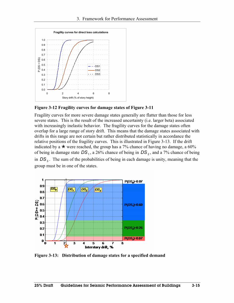
3. Framework for Performance Assessment
25% Draft Guidelines for Seismic Performance Assessment of Buildings 3-15
Fragility curves for direct loss calculations
0.0
0.1
0.2
0.3
0.4
0.5
0.6
0.7
0.8
0.9
1.0
0 2 4 6 8
Story drift (% of story height)
P (D
S >
DSi
)
DS1DS2DS3
Figure 3-12 Fragility curves for damage states of Figure 3-11 Fragility curves for more severe damage states generally are flatter than those for less severe states. This is the result of the increased uncertainty (i.e. larger beta) associated with increasingly inelastic behavior. The fragility curves for the damage states often overlap for a large range of story drift. This means that the damage states associated with drifts in this range are not certain but rather distributed statistically in accordance the relative positions of the fragility curves. This is illustrated in Figure 3-13. If the drift indicated by a were reached, the group has a 7% chance of having no damage, a 60% of being in damage state 1DS , a 26% chance of being in 2DS , and a 7% chance of being in 3DS . The sum of the probabilities of being in each damage is unity, meaning that the group must be in one of the states.
Figure 3-13: Distribution of damage states for a specified demand
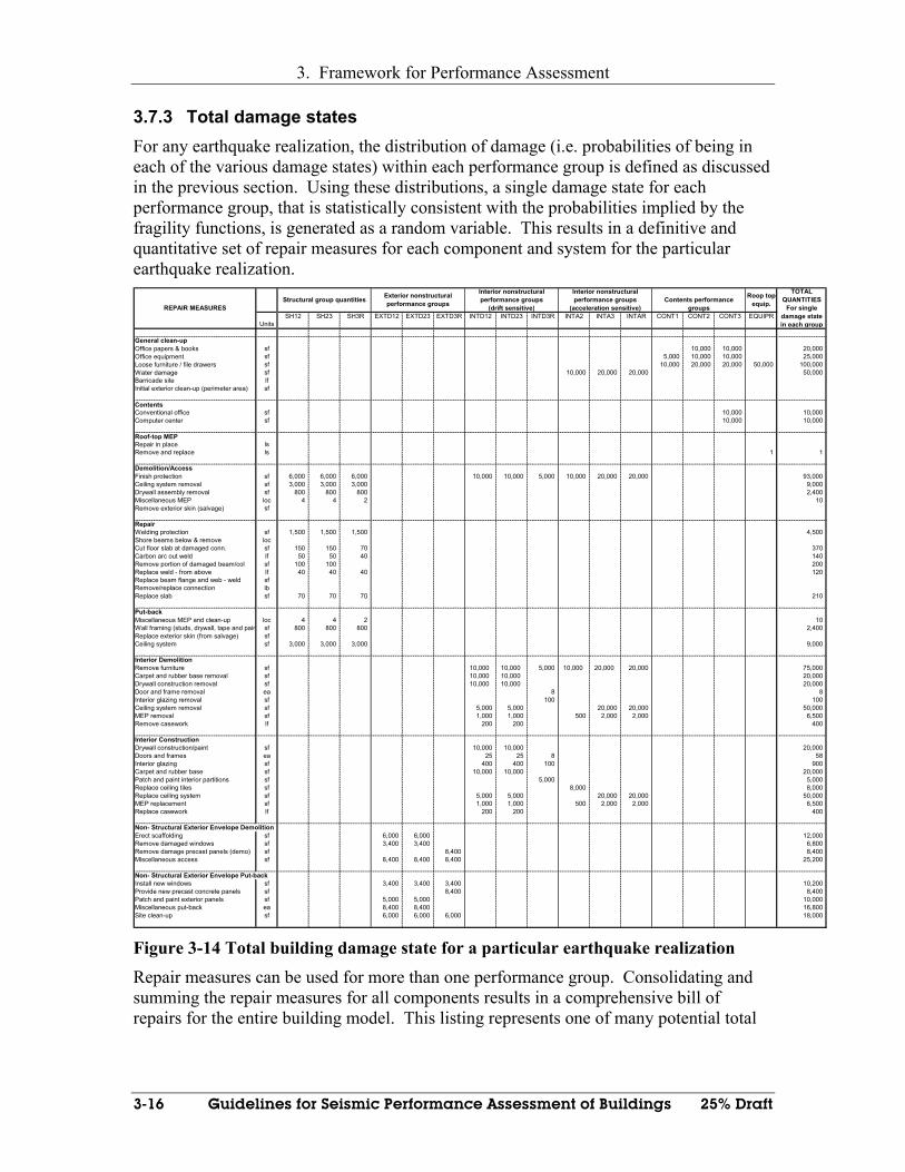
3. Framework for Performance Assessment
3-16 Guidelines for Seismic Performance Assessment of Buildings 25% Draft
3.7.3 Total damage states For any earthquake realization, the distribution of damage (i.e. probabilities of being in each of the various damage states) within each performance group is defined as discussed in the previous section. Using these distributions, a single damage state for each performance group, that is statistically consistent with the probabilities implied by the fragility functions, is generated as a random variable. This results in a definitive and quantitative set of repair measures for each component and system for the particular earthquake realization.
SH12 SH23 SH3R EXTD12 EXTD23 EXTD3R INTD12 INTD23 INTD3R INTA2 INTA3 INTAR CONT1 CONT2 CONT3 EQUIPRUnits
General clean-upOffice papers & books sf 10,000 10,000 20,000Office equipment sf 5,000 10,000 10,000 25,000Loose furniture / file drawers sf 10,000 20,000 20,000 50,000 100,000Water damage sf 10,000 20,000 20,000 50,000Barricade site lfInitial exterior clean-up (perimeter area) sf
ContentsConventional office sf 10,000 10,000Computer center sf 10,000 10,000
Roof-top MEPRepair in place lsRemove and replace ls 1 1
Demolition/AccessFinish protection sf 6,000 6,000 6,000 10,000 10,000 5,000 10,000 20,000 20,000 93,000Ceiling system removal sf 3,000 3,000 3,000 9,000Drywall assembly removal sf 800 800 800 2,400Miscellaneous MEP loc 4 4 2 10Remove exterior skin (salvage) sf
Repair Welding protection sf 1,500 1,500 1,500 4,500Shore beams below & remove locCut floor slab at damaged conn. sf 150 150 70 370Carbon arc out weld lf 50 50 40 140Remove portion of damaged beam/col sf 100 100 200Replace weld - from above lf 40 40 40 120Replace beam flange and web - weld sfRemove/replace connection lbReplace slab sf 70 70 70 210
Put-backMiscellaneous MEP and clean-up loc 4 4 2 10Wall framing (studs, drywall, tape and pain sf 800 800 800 2,400Replace exterior skin (from salvage) sfCeiling system sf 3,000 3,000 3,000 9,000
Interior Demolition Remove furniture sf 10,000 10,000 5,000 10,000 20,000 20,000 75,000Carpet and rubber base removal sf 10,000 10,000 20,000Drywall construction removal sf 10,000 10,000 20,000Door and frame removal ea 8 8Interior glazing removal sf 100 100Ceiling system removal sf 5,000 5,000 20,000 20,000 50,000MEP removal sf 1,000 1,000 500 2,000 2,000 6,500Remove casework lf 200 200 400
Interior ConstructionDrywall construction/paint sf 10,000 10,000 20,000Doors and frames ea 25 25 8 58Interior glazing sf 400 400 100 900Carpet and rubber base sf 10,000 10,000 20,000Patch and paint interior partitions sf 5,000 5,000Replace ceiling tiles sf 8,000 8,000Replace ceiling system sf 5,000 5,000 20,000 20,000 50,000MEP replacement sf 1,000 1,000 500 2,000 2,000 6,500Replace casework lf 200 200 400
Non- Structural Exterior Envelope DemolitionErect scaffolding sf 6,000 6,000 12,000Remove damaged windows sf 3,400 3,400 6,800Remove damage precast panels (demo) sf 8,400 8,400Miscellaneous access sf 8,400 8,400 8,400 25,200
Non- Structural Exterior Envelope Put-backInstall new windows sf 3,400 3,400 3,400 10,200Provide new precast concrete panels sf 8,400 8,400Patch and paint exterior panels sf 5,000 5,000 10,000Miscellaneous put-back ea 8,400 8,400 16,800Site clean-up sf 6,000 6,000 6,000 18,000
Roop top equip.
TOTAL QUANTITIES
For single damage state in each group
REPAIR MEASURESStructural group quantities Exterior nonstructural
performance groups
Interior nonstructural performance groups
(drift sensitive)
Interior nonstructural performance groups
(acceleration sensitive)Contents performance
groups
Figure 3-14 Total building damage state for a particular earthquake realization Repair measures can be used for more than one performance group. Consolidating and summing the repair measures for all components results in a comprehensive bill of repairs for the entire building model. This listing represents one of many potential total
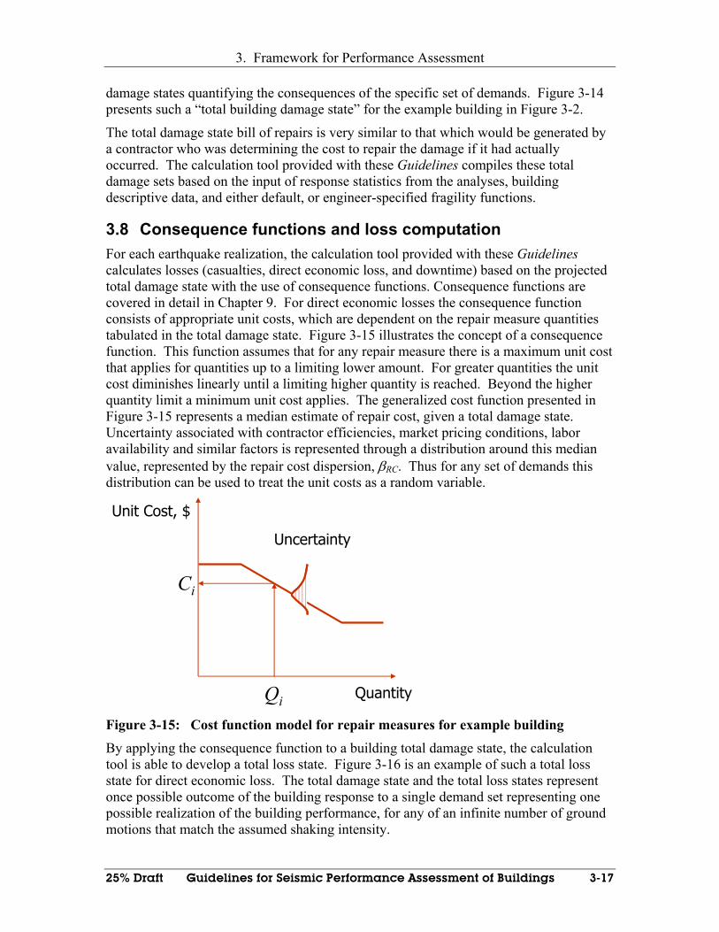
3. Framework for Performance Assessment
25% Draft Guidelines for Seismic Performance Assessment of Buildings 3-17
damage states quantifying the consequences of the specific set of demands. Figure 3-14 presents such a “total building damage state” for the example building in Figure 3-2.
The total damage state bill of repairs is very similar to that which would be generated by a contractor who was determining the cost to repair the damage if it had actually occurred. The calculation tool provided with these Guidelines compiles these total damage sets based on the input of response statistics from the analyses, building descriptive data, and either default, or engineer-specified fragility functions.
3.8 Consequence functions and loss computation For each earthquake realization, the calculation tool provided with these Guidelines calculates losses (casualties, direct economic loss, and downtime) based on the projected total damage state with the use of consequence functions. Consequence functions are covered in detail in Chapter 9. For direct economic losses the consequence function consists of appropriate unit costs, which are dependent on the repair measure quantities tabulated in the total damage state. Figure 3-15 illustrates the concept of a consequence function. This function assumes that for any repair measure there is a maximum unit cost that applies for quantities up to a limiting lower amount. For greater quantities the unit cost diminishes linearly until a limiting higher quantity is reached. Beyond the higher quantity limit a minimum unit cost applies. The generalized cost function presented in Figure 3-15 represents a median estimate of repair cost, given a total damage state. Uncertainty associated with contractor efficiencies, market pricing conditions, labor availability and similar factors is represented through a distribution around this median value, represented by the repair cost dispersion, βRC. Thus for any set of demands this distribution can be used to treat the unit costs as a random variable.
Unit Cost, $
Quantity
Ci
Qi
Uncertainty
Figure 3-15: Cost function model for repair measures for example building
By applying the consequence function to a building total damage state, the calculation tool is able to develop a total loss state. Figure 3-16 is an example of such a total loss state for direct economic loss. The total damage state and the total loss states represent once possible outcome of the building response to a single demand set representing one possible realization of the building performance, for any of an infinite number of ground motions that match the assumed shaking intensity.
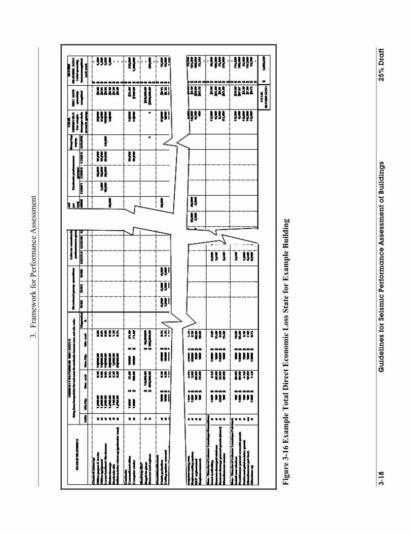
3.
Fra
mew
ork
for P
erfo
rman
ce A
sses
smen
t
3-18
G
uid
eli
ne
s fo
r Se
ism
ic P
erf
orm
an
ce
Ass
ess
me
nt
of
Bu
ild
ing
s 25
% D
raft
Figu
re 3
-16
Exa
mpl
e T
otal
Dir
ect E
cono
mic
Los
s Sta
te fo
r E
xam
ple
Bui
ldin
g
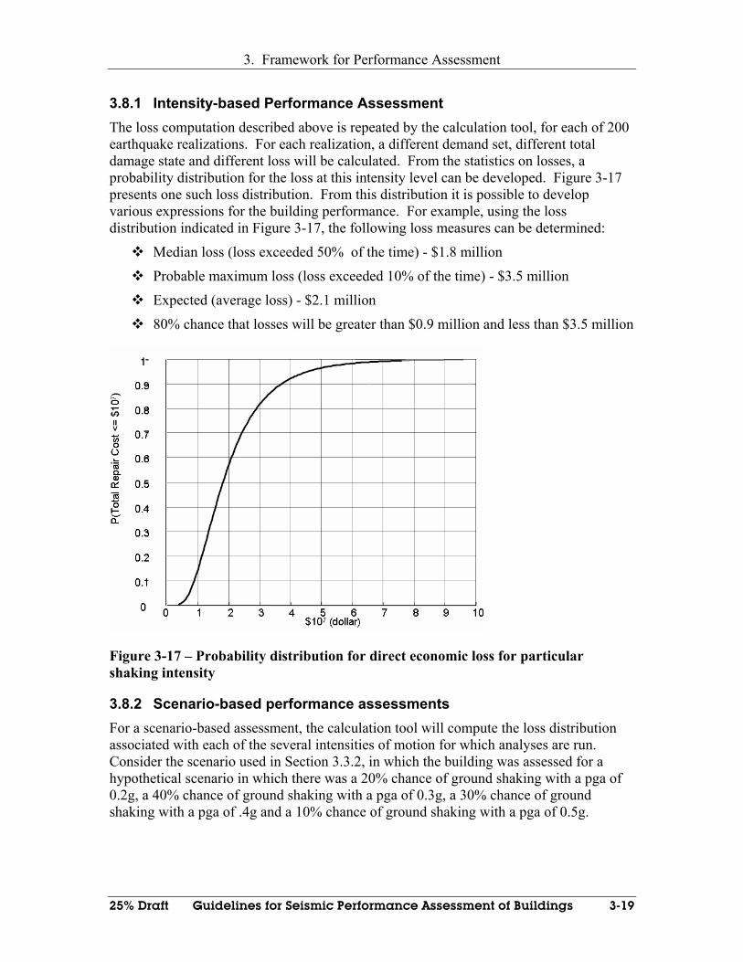
3. Framework for Performance Assessment
25% Draft Guidelines for Seismic Performance Assessment of Buildings 3-19
3.8.1 Intensity-based Performance Assessment The loss computation described above is repeated by the calculation tool, for each of 200 earthquake realizations. For each realization, a different demand set, different total damage state and different loss will be calculated. From the statistics on losses, a probability distribution for the loss at this intensity level can be developed. Figure 3-17 presents one such loss distribution. From this distribution it is possible to develop various expressions for the building performance. For example, using the loss distribution indicated in Figure 3-17, the following loss measures can be determined:
Median loss (loss exceeded 50% of the time) - $1.8 million
Probable maximum loss (loss exceeded 10% of the time) - $3.5 million
Expected (average loss) - $2.1 million
80% chance that losses will be greater than $0.9 million and less than $3.5 million
Figure 3-17 – Probability distribution for direct economic loss for particular shaking intensity
3.8.2 Scenario-based performance assessments For a scenario-based assessment, the calculation tool will compute the loss distribution associated with each of the several intensities of motion for which analyses are run. Consider the scenario used in Section 3.3.2, in which the building was assessed for a hypothetical scenario in which there was a 20% chance of ground shaking with a pga of 0.2g, a 40% chance of ground shaking with a pga of 0.3g, a 30% chance of ground shaking with a pga of .4g and a 10% chance of ground shaking with a pga of 0.5g.

3. Framework for Performance Assessment
3-20 Guidelines for Seismic Performance Assessment of Buildings 25% Draft
Figure 3-18 Direct economic losses for four intensities of ground shaking representing a scenario The direct economic loss distribution for each of these intensities could be as illustrated in Figure 3-18. In the figure, there is a 20% probability that the loss distribution associated with the 0.2g intensity is appropriate, a 40% chance that the loss distribution associated with the 0.3g intensity is appropriate, a 30% chance that the losses associated with the 0.4g intensity is appropriate, and a 10% chance that the losses associated with the 0.5g intensity are appropriate, given that the scenario earthquake, occurs. The calculation tool will combine these statistics to provide a combined loss distribution for the scenario.
0
0.1
0.2
0.3
0.4
0.5
0.6
0.7
0.8
0.9
1
0 0.2 0.4 0.6 0.8 1 1.2 1.4 1.6 1.8 2
Scenario Loss $1,000,000
Prob
abili
ty o
f Non
exce
edan
ce
Figure 3-19 Example scenario direct loss distribution A combined loss distribution is illustrated in Figure 3-19. From such a distribution, it is possible to identify different measures of performance such as the median scenario loss,

3. Framework for Performance Assessment
25% Draft Guidelines for Seismic Performance Assessment of Buildings 3-21
the probable maximum scenario loss, expected scenario loss, etc. in a manner similar to that previously discussed for intensity-based assessments.
3.8.3 Time-based performance assessment A time-based performance assessment requires the generation of cumulative loss function curves for a minimum of four levels of intensity (i.e. 10% chance of being exceed in 5, 10, 50, and 100 year). The complement of each of the cumulative loss functions are then multiplied by the slope of the hazard curve at the corresponding intensity level, and integrated to generate an aggregated loss function relating losses from any seismic shaking to the corresponding annual probability of exceeding the loss. Figure 3-20 illustrates an aggregated direct economic loss function for the example building depicted in Figure 3-2. Time-based assessments in the example used this aggregated loss function. It can be converted to single performance measure by integrating the relationship, as shown in Figure 3-21, to determine the loss expected to occur from seismic shaking annually (i.e. annualized loss). This parameter might be used to judge acceptability in a standard or code. For example, to control damage in critical buildings, a future code might restrict annualized losses to a defined maximum value in terms of replacement cost. This might replace the current importance factor as a more meaningful measure.
0 0.5 1 1.5 2 2.5 3 3.5 4
x 106
0
0.05
0.1
0.15
0.2
0.25
$C (dollar)
Anu
al R
ate
of E
xcee
ding
Tot
al R
epai
r C
ost
= $
C
SMRFX - Sa (0.1395g ~ 0.8305g)
Figure 3-20 Time-based direct economic loss function for example building

3. Framework for Performance Assessment
3-22 Guidelines for Seismic Performance Assessment of Buildings 25% Draft
0.5 1 1.5 2 2.5 3 3.5 40
0.05
0.1
0.15
0.2
0.25
Capital losses ($M)
Annual probability of being exceeded
Area represents expected losses per year (annualized loss)
0.5 1 1.5 2 2.5 3 3.5 40
0.05
0.1
0.15
0.2
0.25
Capital losses ($M)
Annual probability of being exceeded
Area represents expected losses per year (annualized loss)
Figure 3-21: Conversion of aggregated loss function to annualized loss
Annualized losses can be converted to very useful information for decision making on the part of stakeholders. For example, suppose that the curves in Figure 3-22 represent losses associated with a building before and after a proposed retrofit. The reduction in annualized losses from $100k to $60k represents an annualized benefit of $40k per year. Using simple and conventional economic analysis techniques can place this benefit in practical perspective. For example, considering a discount rate (cost on money) of 7% this benefit stream of $40k per year has a net present value (equivalent lump sum today) of $550k over a fifty-year life of the building. Suppose that the retrofit cost in current dollars is $300k. Based on direct economic losses only, the ratio of benefit to costs would then be 1.8, indicating that the retrofit is economically viable. Another form of the same basic information is the rate of return on the investment in retrofit. This is simply annualized benefit divided by the $300k cost of the retrofit, or 13%. An owner can compare this to the return that might be expected from alternative investments for decision-making purposes.
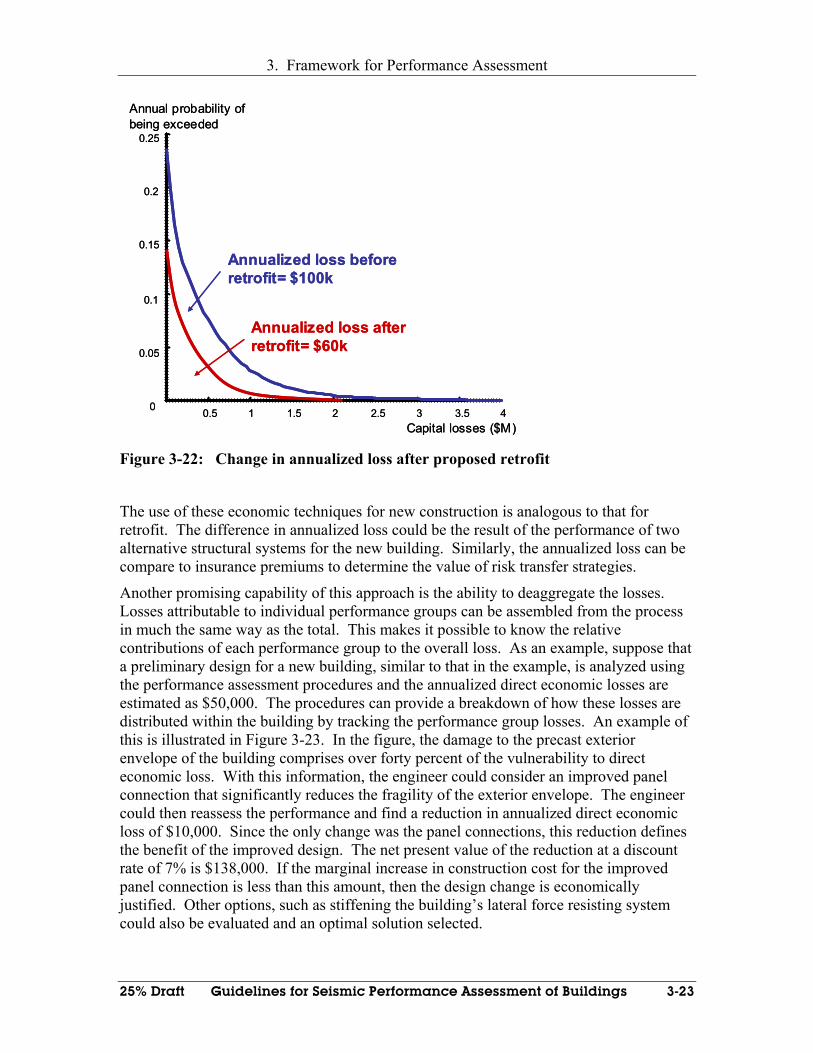
3. Framework for Performance Assessment
25% Draft Guidelines for Seismic Performance Assessment of Buildings 3-23
0.5 1 1.5 2 2.5 3 3.5 40
0.05
0.1
0.15
0.2
0.25
Capital losses ($M)
Annual probability of being exceeded
Annualized loss before retrofit= $100k
Annualized loss after retrofit= $60k
0.5 1 1.5 2 2.5 3 3.5 40
0.05
0.1
0.15
0.2
0.25
Capital losses ($M)
Annual probability of being exceeded
Annualized loss before retrofit= $100k
Annualized loss after retrofit= $60k
Figure 3-22: Change in annualized loss after proposed retrofit
The use of these economic techniques for new construction is analogous to that for retrofit. The difference in annualized loss could be the result of the performance of two alternative structural systems for the new building. Similarly, the annualized loss can be compare to insurance premiums to determine the value of risk transfer strategies.
Another promising capability of this approach is the ability to deaggregate the losses. Losses attributable to individual performance groups can be assembled from the process in much the same way as the total. This makes it possible to know the relative contributions of each performance group to the overall loss. As an example, suppose that a preliminary design for a new building, similar to that in the example, is analyzed using the performance assessment procedures and the annualized direct economic losses are estimated as $50,000. The procedures can provide a breakdown of how these losses are distributed within the building by tracking the performance group losses. An example of this is illustrated in Figure 3-23. In the figure, the damage to the precast exterior envelope of the building comprises over forty percent of the vulnerability to direct economic loss. With this information, the engineer could consider an improved panel connection that significantly reduces the fragility of the exterior envelope. The engineer could then reassess the performance and find a reduction in annualized direct economic loss of $10,000. Since the only change was the panel connections, this reduction defines the benefit of the improved design. The net present value of the reduction at a discount rate of 7% is $138,000. If the marginal increase in construction cost for the improved panel connection is less than this amount, then the design change is economically justified. Other options, such as stiffening the building’s lateral force resisting system could also be evaluated and an optimal solution selected.
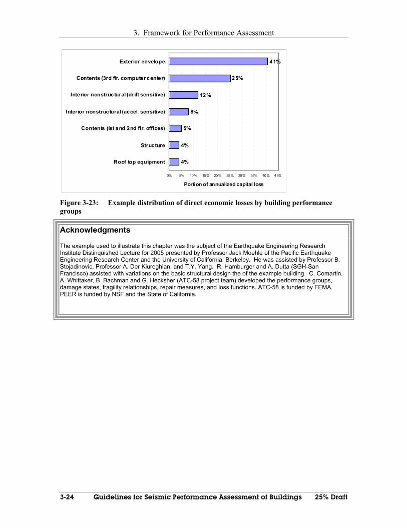
3. Framework for Performance Assessment
3-24 Guidelines for Seismic Performance Assessment of Buildings 25% Draft
4%
4%
5%
8%
12%
25%
41%
0% 5% 10% 15% 20% 25% 30% 35% 40% 45%
Roof top equipment
Structure
Contents (Ist and 2nd flr. offices)
Interior nonstructural (accel. sensitive)
Interior nonstructural (drift sensitive)
Contents (3rd flr. computer center)
Exterior envelope
Portion of annualized capital loss
Figure 3-23: Example distribution of direct economic losses by building performance groups
Acknowledgments
The example used to illustrate this chapter was the subject of the Earthquake Engineering Research Institute Distinquished Lecture for 2005 presented by Professor Jack Moehle of the Pacific Earthquake Engineering Research Center and the University of California, Berkeley. He was assisted by Professor B. Stojadinovic, Professor A. Der Kiureghian, and T.Y. Yang. R. Hamburger and A. Dutta (SGH-San Francisco) assisted with variations on the basic structural design the of the example building. C. Comartin, A. Whittaker, B. Bachman and G. Hecksher (ATC-58 project team) developed the performance groups, damage states, fragility relationships, repair measures, and loss functions. ATC-58 is funded by FEMA. PEER is funded by NSF and the State of California.
25% Draft Guidelines for Seismic Performance Assessment of Buildings 4-1
4 Building Definition
4.1 Introduction The first step in the performance assessment process is the definition of the building’s composition. In this Chapter, the specific information that is to be identified and defined for the building is described. This information includes the building’s usage and occupancy, its location and site conditions and identification of the structural and nonstructural systems. The identification of systems includes specifying their unique characteristics, their dimensions and weights, their distribution throughout the building, their costs and their potential impact on building occupancy, use, and life safety if they were to be damaged in an earthquake. The identification of these items in a systematic way defines the potential exposure to loss. The description of the building’s construction and occupancy is to be provided in sufficient detail that a relatively accurate assessment of repair costs, repair and service restoration times, and casualties can be made once a determination of the building’s response and damage has been performed. The degree of detail that is to be included in the building definition varies with the level of performance assessment that is planned and the availability of information. For example, in early stages of conceptual design, only very cursory information may be available regarding the structural and nonstructural systems while at the construction documents stage or for assessments of existing buildings very detailed information may be available.
It is important is that the necessary data to define the building be collected and assembled in a logical and useful format. This chapter provides guidelines for the collection of the required data.
4.2 Building Occupancy, Function and Contents Identify the intended building use. This usage is identified by the term occupancy. Buildings are used in a wide range of occupancies. Each occupancy has unique characteristics, nonstructural systems and components, intensity of use and contents. All of these unique features affect the losses that occur due to earthquake damage. These Guidelines include default inventory, damage and loss data for several common building occupancies:
• Commercial Office
• Education
• Healthcare
• Hospitality
• Residential
• Research
• Retail
• Warehouse

4. Building Definition
4-2 Guidelines for Seismic Performance Assessment of Buildings 25% Draft
It is possible to override the default data for these occupancies by providing user -defined information. It is also possible to use this same feature to perform assessments of buildings that are in different occupancies than those indicated above, by specifying user-defined information.
In addition to the building occupancy type, identify the number of people who would typically occupy the building, and the typical times of the day and week during which this occupancy occurs. This information is used to estimate potential casualities.
Identify critical functional requirements located within the building. Also identify costs or consequences associated with downtime of particular building functions. For example, continued operation of a computer data center within a building may be essential to business operations, and loss of operation of that data center could result in financial consequences to the business.
Identify important contents, which are, or will be, located within the building. Contents that are important to critical functional requirements are also to be noted. For example, damage to a museum artifact or valuable inventory could lead to significant dollar losses. Loss of computer usage could cause dollar losses due to repair or replacement in addition to losses associated with downtime.
4.3 Site considerations
4.3.1 Seismic Environment and Hazard Use the procedures of Chapter 5 to establish the seismic hazard due to ground shaking for a given building and site. The hazard characterization is based on the location of the building with respect to causative faults, the regional and site-specific geologic characteristics, local topographic conditions and the selected representation of ground shaking (for intensity-based, scenario-based and time-based assessments).
In addition to ground shaking, the building performance can be affected substantially by other earthquake-induced geologic hazards. Introductory information on these hazards is presented in Section 4.3.4 below and Kramer (1996). However, procedures for assessing the effect of these other geologic hazards on building performance are not presented in these Guidelines at this time.
4.3.2 Location For scenario (magnitude, distance and source) estimates of the shaking, define the distance from the building site to the causative fault so that attenuation relationships (see Section 5.4.3) can be used to estimate the ground shaking intensity associate with the scenario. For time-based assessments, define the exact location of the building site to permit determination of the seismic hazard. The seismic hazard will be determined using the General Procedures of Section 5.3 or the Probabilistic Seismic Hazard Analysis (PSHA) procedures of Section 5.4. In either case, latitude and longitude are used to identify the coordinates of the site. Three significant digits (after the decimal point) are sufficient to identify the latitude and longitude.

4. Building Definition
25% Draft Guidelines for Seismic Performance Assessment of Buildings 4-3
4.3.3 Site Soil and Topographic Conditions Define the properties of the soil at the building site for all performance assessments. For scenario assessments, classify the soil in a manner (e.g., rock, stiff soil, shear wave velocity in the upper 30 meters) consistent with the attenuation relationship(s) used for the hazard characterization. For intensity-based assessments and time-based assessments, categorize the site in terms of site class per Section 5.3 so that appropriate spectra can be defined. For those assessments in which soil-structure-foundation interaction analyses are performed, nonlinear stress-strain or constitutive relationships of the soils materials will be required as well.
Local topographic conditions (e.g., hills, valleys, canyons) will modify the amplitude, frequency content and duration of earthquake strong motion relative to that expected at a flat, level site in the free-field. Finite-element and finite-difference numerical tools can be used to characterize the influence of topographic effects on earthquake shaking on such sites.
4.3.4 Geologic Site Hazards The assessment and loss-calculation procedures presented in these Guidelines are focused on buildings subjected to earthquake shaking. However, other seismic hazards may exist at the building site that could damage the building regardless of its ability to resist ground shaking. These hazards include fault rupture, liquefaction, lateral spreading, landslides, and inundation from offsite effects such as dam failure or tsunami. Each of these hazards could substantially affect building performance. The framework presented in these Guidelines is applicable in principle to these other geologic hazards however; the specific procedure for assessing the performance affects of these hazards is not included herein.
Buildings that straddle active faults should be assessed for the likely amount and direction of ground surface rupture. Geologic information is needed for this assessment, including 1) the degree of activity based on the age of most recent movement, 2) fault type (strike-slip, normal-slip, reverse slip or thrust fault); 3) the angle of slip with respect to the building plan footprint; 4) magnitudes of movement expected for the chosen hazard (intensity-based, scenario-based or time-based); and 5) the width of the fault-rupture zone.
Soil liquefaction is a phenomenon in which loose, granular soils below the water table lose strength due to strong ground shaking. Recent natural loose or uncompacted granular deposits, or poorly compacted granular fill soils, are especially vulnerable to liquefaction. Dense natural soils, well-compacted fills and clayey soils are generally not susceptible to liquefaction. Geologic information is needed for a liquefaction assessment, includes: depth to the ground water table, soil type, soil density; ground surface slope and proximity of free-face conditions. Soils susceptible to liquefaction are also susceptible to differential compaction and lateral spreading.
Lateral spreading is a phenomenon that occurs on sloping site susceptible to liquefaction. As the site liquefies, the surficial materials begin to flow downhill. Lateral spreading often results in deep fissures in the ground surface and uneven settlement of supported structures. It is highly disrupted of buried utilities.
4. Building Definition
4-4 Guidelines for Seismic Performance Assessment of Buildings 25% Draft
Differential compaction is an earthquake-induced process in which foundation soils (either liquefiable or non-liquefiable) compact and the foundation above settles non-uniformly across the building site. Landsliding is the down-slope mass movement of earth. Subsurface soil data is needed to characterize the potential for differential compaction and landsliding.
Sources of flooding or inundation at a building site include: breech or failure of dams located upstream; pipelines; aqueducts and water storage tanks located upstream, damaged by shaking or non-shaking hazards; tsunamis (coastal areas) and seiches (adjacent to lakes); and low-lying areas with shallow ground water, subject to regional subsidence and surface ponding of water.
4.3.5 Reliability of Utilities The post-earthquake operation and functionality of a building will be dependent on the availability of off-site services, including power, potable water, gas, telecommunications infrastructure and transportation. When performing assessments, the potential effects of loss of these services and utilities on building occupancy and casualties should be considered. Such consideration is outside the scope of these Guidelines.
4.4 Characterization of Structure and Foundations
4.4.1 Introduction Performance assessments may be performed at different phases of a new building design (for example, conceptual design, design development and construction documents) and for a variety of reasons including: computing expected losses, comparing framing systems, and choosing the robustness of nonstructural components and contents. Differing levels of building construction data will be available during the phases of a new building design. Performance assessments can also be performed on existing buildings, either to assess the risk associated with building use or as part of an upgrade design of structural and nonstructural components and contents.
The following subsections identify the minimum level of definition of structural systems necessary to conduct either conceptual or detailed performance assessments using these Guidelines. Alternate assessments, using more information than that required for conceptual assessments (Section 4.4.2) and less information than that which is necessary for detailed assessments (Section 4.4.3) can be undertaken, although explicit guidance for such assessment is not provided herein.
4.4.2 Conceptual Assessment Define the structural framing system for gravity- and earthquake-load resistance must be in sufficient detail to permit the estimation of inter-story drift and floor acceleration at various levels of ground shaking intensity.
A numerical model of the building structure is used to compute statistical estimates (e.g., median, dispersion) of demand on the structural components resulting from horizontal ground shaking. Vertical earthquake shaking and soil-foundation-structure interaction need not be considered for this level of assessment.

4. Building Definition
25% Draft Guidelines for Seismic Performance Assessment of Buildings 4-5
The following structural-framing and subsurface-material information is required for conceptual-level assessment:
• Plan dimensions, bay dimensions, story heights, number of stories, basement data.
• Type of structural framing system (e.g., special steel moment-resisting frame)
• Estimates of the building weight, including structural framing, occupancy-typical non-structural components, and exterior cladding at each floor level of the building.
• Estimates of the stiffness and yield strength of each story
• Subsurface material site class (A through F) per Section 5.3
Two methods of building-response analysis are provided for use in conceptual-level assessments: nonlinear dynamic response analysis per Section 6.3 and linear static response analysis per Section 6.4.
Irrespective of the analysis method used to compute displacement and acceleration demands, each response parameter is assumed to be lognormally distributed with a median value Dθ , mean Dm , standard deviation Dσ , coefficient of variation Dν , and standard deviation of the natural logarithm of the response ln Dσ (which is also denoted
Dβ and termed the dispersion in these Guidelines) The lognormal distribution is fully defined by Dθ and Dβ . Relationships between Dθ , Dm , Dσ , Dν and Dβ are presented in Appendix A.
4.4.3 Detailed Assessment For detailed assessments, nonlinear dynamic nonlinear response history analysis will be used to predict median values and dispersions of demand parameters used to predict damage at different intensity levels.
The following structural-framing and geologic information is required:
• Plan dimensions, bay dimensions, story heights, basement data.
• Sizes (depth, weight/length, thickness, rebar) and geometry of all components of the gravity-load and earthquake-resisting framing systems.
• Details of all beam-column (-wall), beam-brace, beam-link, column base plate-foundation, column-brace base plate-foundation, and wall-foundation connections
• Building weight, including structural framing, non-structural components and equipment, and exterior cladding at each floor level of the building.
• Sizes of foundation elements, including footings; mats; pile caps; pile diameter and length, and load-resisting mechanism; foundation embedment.
• For structures in which soil-foundation-structure interaction effects are significant, impedance functions for the foundation-soil system; shear-wave velocity and effective strain-degraded shear modulus in the subsurface materials beneath the foundation to a depth equal to the maximum building footprint

4. Building Definition
4-6 Guidelines for Seismic Performance Assessment of Buildings 25% Draft
dimension; foundation soil springs and dashpots; stress-strain or constitutive models for the soil layers underlying the foundation; frequency-dependent boundary stiffness and damping matrices for the edges (boundaries) of a finite element model of the subsurface materials beneath the building.
4.5 Nonstructural Systems and Components Modeling
4.5.1 Classification Scheme The potential vulnerability of individual nonstructural components and systems to earthquake motions is a function of many factors. The most reliable way of assessing a component’s vulnerability to various types and intensities of shaking is by laboratory testing of prototypes. In some cases, component suppliers have performed such testing, either at the request of specific customers, or to obtain a general understanding of the vulnerability of their products. Some universities have also performed such testing, to study the likely performance of common building systems. Finally, some industry groups, such as the commercial power generation industry have also sponsored such tests as well as collected data on the performance of installed components and systems in earthquakes. However, for many components and systems found in buildings, this data does not exist. For such components, judgmental data must be used until other sources of data become available.
Because of the wide range and quantity of nonstructural systems and components found in typical buildings, it would not be practical to attempt to assess the performance of each individual component and system. Instead, broad collections of components and systems that have similar damageability, similar consequences with regard to loss and are subjected to similar shaking demands within a building are assembled into sets, termed performance groups. These performance groups, rather than the individual components that comprise them, are then evaluated for their probable performance, as a group.
These Guidelines include default performance groups that incorporate the typical non- structural components and systems common to the standard occupancies described above. The performance groups are indexed to the quality of seismic-resistant features with which the systems are installed, as well as the age and style of construction since these features and attributes have been found to greatly affect the damage susceptibility of these nonstructural building elements. Typically it will be necessary to identity different performance groups on each floor or story of the building, as the intensity of shaking effects will likely vary throughout the structure’s height. For existing buildings, it may also be necessary to identify unique performance groups within different tenant suites, if the style and age of construction varies significantly throughout the building. Also more recent building codes, prescribe different design requirements within the relative height of a building so that the capacity of typical nonstructural systems may increase with vertical location.
The assessment process includes the concept of presumed default values types and quantities of nonstructural components for the range of occupancies considered and size of building. Therefore if detailed information regarding nonstructural components is not available, it is still possible to perform a performance assessment using default values. The process also permits specific types and quantities to be substituted for default values
4. Building Definition
25% Draft Guidelines for Seismic Performance Assessment of Buildings 4-7
when such data is available. However, any values substituted for default values require adequate substantiation and review since specialty expertise is required to establish fragility characteristics.
4.5.1.1 Level of Assessment
There are two levels of performance assessment for nonstructural components that are related to the quality of information typically available at different project stages. These are:
1. Conceptual Level – For this level, very little information is needed about the nonstructural systems other than the basic building occupancy and size, and the age and quality of installation of nonstructural systems. At this level, default options are typically used to describe nonstructural components and quantities. Due to the vague definition of nonstructural systems in this level, performance assessments made using this level of data will be quite uncertain.
2. Detailed Level – For this level of assessment, the nonstructural systems are defined to the same degree as might be found in construction documents. Quantities are based on take offs from construction drawings and detailed requirements for nonstructural systems are taken from specifications and drawings. Assessments made using this level of data will have the least uncertainty.
4.5.1.2 Year of Installation
Because codes, standards and installation practices have changed over time, the seismic vulnerability of nonstructural components are significantly influenced by the year they were installed. To permit the effect of year of installation to be included in the assessment in an organized way, the year of installation should be identified and classified into one of the following categories:
• 1950’s or prior
• 1960’s
• 1970’s
• 1980’s
• 1990’s
• 2000’s
4.5.1.3 Seismic Practice
The seismic practice used in the installation is also very important especially for assessment of existing buildings. The design and installation requirements for nonstructural components vary considerably, depending on geographic region and seismicity. In some portions of the United States seismic requirements for nonstructural components have routinely been neglected even though they were required by locally adopted building codes. This seismic practice dependency needs to be considered in the
4. Building Definition
4-8 Guidelines for Seismic Performance Assessment of Buildings 25% Draft
assessment. Typically the seismic practice can be grouped according to the building code requirements under which a structure was constructed, as follows:
1. Group 1 – Uniform Building Code Zone 3 and 4
2. Group 2 –Uniform Building Code Zone 2A and 2B
3. Group 3 – Uniform Building Code Zone 0 and 1
4. Group 4 - Seismic Design Category A
5. Group 5 - Seismic Design Category B
6. Group 6 - Seismic Design Category C
7. Group 7 - Seismic Design Category D, E, or F
4.5.1.4 Installation Quality Assurance
The level of quality assurance that occurred or will occur in the installation process also has a significant influence on seismic vulnerability of nonstructural components. Assign one of the following levels of quality assurance:
1. Quality Level 1 – Highest Level of Inspection – equivalent to a nuclear facility
2. Quality Level 2 – Building Code Essential Facility Inspection – equivalent to California Hospital Practice
3. Quality Level 3 - Commercial special inspection – higher level of inspection specifically done for nonstructural components in accordance with code requirements
4. Quality Level 4 – Structural Observation inspection – minor inspection – however not as thorough as commercial special inspection
5. Quality Level 5 – Level of Quality Assurance unknown – probably none
4.5.1.5 Facility Seismic Safety Management
The level of facility seismic safety management that will likely occur (or is occurring) in the building after it is occupied also can have a significant influence of the seismic vulnerability of nonstructural components and especially contents. Assign one of the following levels of facility seismic management:
1. Management Level 1 – Highest Level of Management Priority - All contents secured, bookcases anchored to walls, contents in shelves secured, computers and monitors are secured, inspections done in ceilings after repairs to be sure seismic bracing is left in place. Purchased storage racks meet current seismic code requirements. Personnel trained for seismic safety and it is a culture of the occupying organization. Full buy-in by occupying staff
2. Management Level 2 – Moderate Level of Management Priority – limited securing of contents, no lips for bookshelves, personnel safety training is an individual responsibility. Purchased storage racks meet current seismic code requirements only if required by local authority. More likely to occur in higher seismic areas.
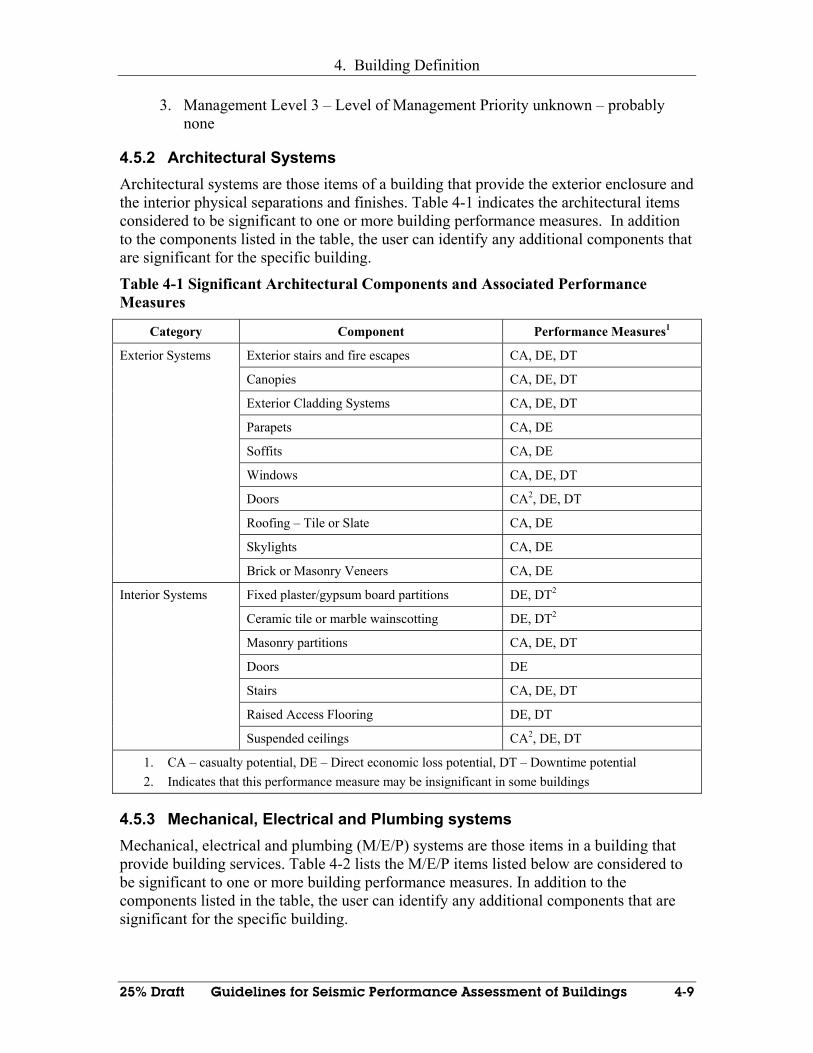
4. Building Definition
25% Draft Guidelines for Seismic Performance Assessment of Buildings 4-9
3. Management Level 3 – Level of Management Priority unknown – probably none
4.5.2 Architectural Systems Architectural systems are those items of a building that provide the exterior enclosure and the interior physical separations and finishes. Table 4-1 indicates the architectural items considered to be significant to one or more building performance measures. In addition to the components listed in the table, the user can identify any additional components that are significant for the specific building.
Table 4-1 Significant Architectural Components and Associated Performance Measures
Category Component Performance Measures1
Exterior stairs and fire escapes CA, DE, DT
Canopies CA, DE, DT
Exterior Cladding Systems CA, DE, DT
Parapets CA, DE
Soffits CA, DE
Windows CA, DE, DT
Doors CA2, DE, DT
Roofing – Tile or Slate CA, DE
Skylights CA, DE
Exterior Systems
Brick or Masonry Veneers CA, DE
Fixed plaster/gypsum board partitions DE, DT2
Ceramic tile or marble wainscotting DE, DT2
Masonry partitions CA, DE, DT
Doors DE
Stairs CA, DE, DT
Raised Access Flooring DE, DT
Interior Systems
Suspended ceilings CA2, DE, DT
1. CA – casualty potential, DE – Direct economic loss potential, DT – Downtime potential 2. Indicates that this performance measure may be insignificant in some buildings
4.5.3 Mechanical, Electrical and Plumbing systems Mechanical, electrical and plumbing (M/E/P) systems are those items in a building that provide building services. Table 4-2 lists the M/E/P items listed below are considered to be significant to one or more building performance measures. In addition to the components listed in the table, the user can identify any additional components that are significant for the specific building.

4. Building Definition
4-10 Guidelines for Seismic Performance Assessment of Buildings 25% Draft
Table 4-2 Significant Mechanical, Electrical and Plumbing Components and Associated Performance Measures
Category Component Performance Measures1
Conveying Systems Elevators and Escalators CA, DE, DT
Domestic Water Distribution DE, DT
Sanitary Waste System DE, DT
Plumbing
Specialty Plumbing such as acid waste, gas, etc.
CA, DE, DT
Chillers DE, DT
Air Handlers DE, DT2
Boilers CA, DE, DT
Building Mechanical Systems
Mechanical piping and ductwork CA2, DE, DT
Sprinkler systems CA2, DE, DT Fire Protection
Standpipes DE, DT
Lighting CA, DE, DT
Convenience DE, DT
Electrical
High voltage DE, DT
1. CA – casualty potential, DE – Direct economic loss potential, DT – Downtime potential 2. indicates that this performance measure may not be significant
4.5.4 Building Contents Building contents are those items housed in the building that are typically supplied by the tenants. They tend to be very much occupancy dependent. If the building being assessed is just a shell or empty offices, the contents will not be included in the assessment. If the tenant owns the building being assessed then contents may be included in the assessment and may be very significant in the assessment. Typically economic losses associated with contents owned by temporary residents of a building such as hotel guests are not included in loss assessments. Table 4-3 lists typical contents classified by occupancy type that are believed to be significant to one or more of the performance measures. In addition to the components listed in the table, the user can identify any additional components that are significant for the specific building.
Table 4-3 Significant Contents and Associated Performance Measures
Occupancy Component Performance Measures1
Desktop Computers (later)
Tall File Cabinets (later)
Business equipment (printers, servers, mainframes, etc)
(later)
Commercial Office
Tall slender book cases (later)
Education Bookshelves (later)

4. Building Definition
25% Draft Guidelines for Seismic Performance Assessment of Buildings 4-11
Desktop computers (later)
Tall File Cabinets (later)
Medical Equipment (later)
Kitchen Equipment (later)
Tall Bookcases (later)
Healthcare
Desktop computers (later)
Hospitality Kitchen Equipment (later)
Desktop computers (later)
Home entertainment Equipment (later)
Residential
China (later)
Storage racks (later)
Tall display racks (later)
Contents on racks (later)
Retail
Cold Rooms (later)
Warehouse Storage racks (later)
Contents on racks (later)
1. CA – casualty potential, DE – Direct economic loss potential, DT – Downtime potential 2. indicates that this performance measure may not be significant
4.5.5 Level of Assessment and Nonstructural Definition Detail
4.5.5.1 Conceptual Level Assessment
For conceptual level assessments it is expected that very little will be known about the architectural, Mechanical/Electrical/Plumbing and contents building items. However, the information on the intended occupancy, estimated year of installation, building location and level of quality inspection should be available and defined as specified in Section 4.5.1. From the basic architectural concept, the floor area and number of stories is expected to be also available. If some additional information is available such as contemplated type of exterior finish, this also can be utilized and substituted for the default assumptions. Based on this basic information, default quantities of the items listed in Section 4.5.2 through 4.5.4 based on architectural design standards will be computed for each floor. These default quantities are presented and discussed in Appendix E. In addition to quantities, default estimated costs of the architectural, Mechanical/Electrical/Plumbing and contents component portions of the building and unit costs for the listed items are also provided in Appendix E. As with quantities, default fragilities are assigned to the above architectural, Mechanical/Electrical/Plumbing and architectural lists. These default fragilities are also presented and discussed in Appendix E.

4. Building Definition
4-12 Guidelines for Seismic Performance Assessment of Buildings 25% Draft
4.5.4.2 Detailed Level Assessment
For detailed level assessments, detailed construction drawings (or walkdown assessments) are assumed to be available along with a construction cost estimate. Detailed quantities of all architectural, Mechanical/Electrical/Plumbing components and contents for each floor are expected to be available or computed. Note that where the quantity of items are greater in one direction than another (for example exterior wall systems of a rectangular narrow building or escalators) quantities are to be independently determined for each direction since they may be more vulnerable in one direction than another. Also the unit costs associated with the items listed in Section 4.5.2 through Section 4.5.4 are to be provided along with unit costs of any other architectural features not listed which are deemed significant. Note that the units of quantity and cost are to be consistent with the level of detail provided in the construction cost estimate. Based on more detailed information provided in drawing details, construction specifications or walkdown assessments, better estimates of fragilities are expected to be used. More detailed available fragilities are provided in Appendix E and in some cases it may be worthwhile to establish fragilities for selected architectural or Mechanical/Electrical/Plumbing components or contents for a given project. Procedures for establishing fragilities are provided in Appendix C.
4.6 Performance Groups
4.6.1 General Because of the wide range and quantity of structural and nonstructural systems and components found in typical buildings, it would not be practical to attempt to assess the performance of each individual component and system. Instead, broad collections of components and systems that have similar damageability, similar consequences with regard to loss and are subjected to similar shaking demands within a building are assembled into sets, termed performance groups. These performance groups, rather than the individual components that comprise them, are then evaluated for their probable performance, as a group.
4.6.2 Structural Performance Groups
4.6.2.1 Introduction
Structural performance groups are defined in terms of critical demand parameters such as shear force, V, and plastic hinge rotation, pθ . Multiple structural components are assigned to a given performance group if those components share a common critical demand parameter as predicted by analysis (e.g., beam-column connections in special steel moment-resisting frames at a particular story of a building and active in a particular framing direction.) Fragility curves are assigned to each component in the performance group. For the purposes of implementation and loss computation, performance groups are assigned by story based on the gravity- and earthquake-framing in that story.
Different structural performance groups are used to compute the different performance measures, i.e., direct losses, casualties and downtime. Default structural performance groups are presented in Section 4.6.2.2 for structural framing systems involving steel
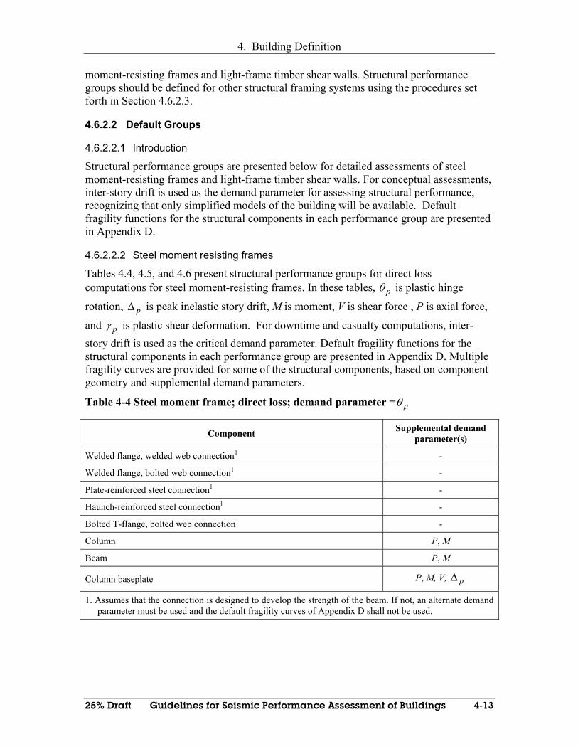
4. Building Definition
25% Draft Guidelines for Seismic Performance Assessment of Buildings 4-13
moment-resisting frames and light-frame timber shear walls. Structural performance groups should be defined for other structural framing systems using the procedures set forth in Section 4.6.2.3.
4.6.2.2 Default Groups
4.6.2.2.1 Introduction
Structural performance groups are presented below for detailed assessments of steel moment-resisting frames and light-frame timber shear walls. For conceptual assessments, inter-story drift is used as the demand parameter for assessing structural performance, recognizing that only simplified models of the building will be available. Default fragility functions for the structural components in each performance group are presented in Appendix D.
4.6.2.2.2 Steel moment resisting frames
Tables 4.4, 4.5, and 4.6 present structural performance groups for direct loss computations for steel moment-resisting frames. In these tables, pθ is plastic hinge
rotation, p∆ is peak inelastic story drift, M is moment, V is shear force , P is axial force,
and pγ is plastic shear deformation. For downtime and casualty computations, inter-story drift is used as the critical demand parameter. Default fragility functions for the structural components in each performance group are presented in Appendix D. Multiple fragility curves are provided for some of the structural components, based on component geometry and supplemental demand parameters.
Table 4-4 Steel moment frame; direct loss; demand parameter = pθ
Component Supplemental demand parameter(s)
Welded flange, welded web connection1 -
Welded flange, bolted web connection1 -
Plate-reinforced steel connection1 -
Haunch-reinforced steel connection1 -
Bolted T-flange, bolted web connection -
Column P, M
Beam P, M
Column baseplate P, M, V, p∆
1. Assumes that the connection is designed to develop the strength of the beam. If not, an alternate demand parameter must be used and the default fragility curves of Appendix D shall not be used.

4. Building Definition
4-14 Guidelines for Seismic Performance Assessment of Buildings 25% Draft
Table 4-5 Steel moment frame; direct loss; demand parameter = pγ
Component Supplemental demand parameter(s)
Panel zone in beam-column joint P
Table 4-6 Steel moment frame; direct loss; demand parameter = M
Component Supplemental demand parameter(s)
Bolted end-plate connection -
Column splices P, V, pθ
Composite slab-on-metal deck pθ
Reinforced concrete foundations P, V, pθ
4.6.2.2.3 Light frame wood shear wall
Tables 4-7, 4-8 and 4-9 present structural performance groups for direct loss computations for light frame wood shear wall construction. In these tables, ∆ is peak story drift, p∆ is peak inelastic story drift, ip∆ is the peak-in-plane deformation, M is moment, V is shear force and P is axial force. For downtime and casualty computations, inter-story drift is used as the critical demand parameter. Default fragility functions for the structural components in each performance group are presented in Appendix D. Multiple fragility curves are provided for some of the structural components, based on component geometry and supplemental demand parameters.
Table 4-7 Light frame wood shear wall; direct loss; demand parameter = ∆
Component Supplemental demand parameter(s)
Plywood walls -
Oriented strand board -
Gypsum wall board -
Exterior plaster-finished walls -
Interior plaster-finished walls -
Posts and studs -
Floor diaphragm P, M, ip∆
Roof diaphragm P, M, ip∆
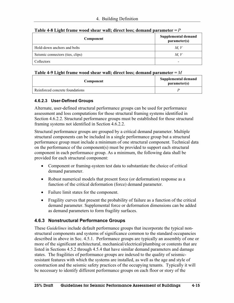
4. Building Definition
25% Draft Guidelines for Seismic Performance Assessment of Buildings 4-15
Table 4-8 Light frame wood shear wall; direct loss; demand parameter = P
Component Supplemental demand parameter(s)
Hold-down anchors and bolts M, V
Seismic connectors (ties, clips) M, V
Collectors -
Table 4-9 Light frame wood shear wall; direct loss; demand parameter = M
Component Supplemental demand parameter(s)
Reinforced concrete foundations P
4.6.2.3 User-Defined Groups
Alternate, user-defined structural performance groups can be used for performance assessment and loss computations for those structural framing systems identified in Section 4.6.2.2. Structural performance groups must be established for those structural framing systems not identified in Section 4.6.2.2.
Structural performance groups are grouped by a critical demand parameter. Multiple structural components can be included in a single performance group but a structural performance group must include a minimum of one structural component. Technical data on the performance of the component(s) must be provided to support each structural component in each performance group. As a minimum, the following data shall be provided for each structural component:
• Component or framing-system test data to substantiate the choice of critical demand parameter.
• Robust numerical models that present force (or deformation) response as a function of the critical deformation (force) demand parameter.
• Failure limit states for the component.
• Fragility curves that present the probability of failure as a function of the critical demand parameter. Supplemental force or deformation dimensions can be added as demand parameters to form fragility surfaces.
4.6.3 Nonstructural Performance Groups These Guidelines include default performance groups that incorporate the typical non- structural components and systems of significance common to the standard occupancies described in above in Sec. 4.5.1. Performance groups are typically an assembly of one or more of the significant architectural, mechanical/electrical/plumbing or contents that are listed in Sections 4.5.2 through 4.5.4 that have similar demand parameters and damage states. The fragilities of performance groups are indexed to the quality of seismic-resistant features with which the systems are installed, as well as the age and style of construction and the seismic safety practices of the occupying tenants. Typically it will be necessary to identify different performance groups on each floor or story of the
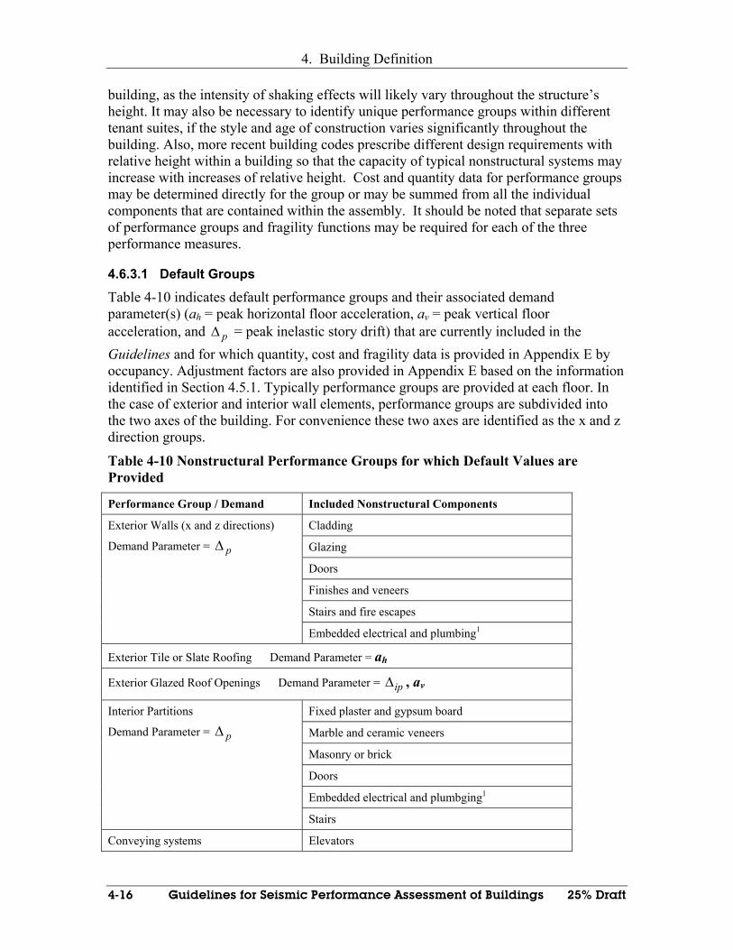
4. Building Definition
4-16 Guidelines for Seismic Performance Assessment of Buildings 25% Draft
building, as the intensity of shaking effects will likely vary throughout the structure’s height. It may also be necessary to identify unique performance groups within different tenant suites, if the style and age of construction varies significantly throughout the building. Also, more recent building codes prescribe different design requirements with relative height within a building so that the capacity of typical nonstructural systems may increase with increases of relative height. Cost and quantity data for performance groups may be determined directly for the group or may be summed from all the individual components that are contained within the assembly. It should be noted that separate sets of performance groups and fragility functions may be required for each of the three performance measures.
4.6.3.1 Default Groups
Table 4-10 indicates default performance groups and their associated demand parameter(s) (ah = peak horizontal floor acceleration, av = peak vertical floor acceleration, and p∆ = peak inelastic story drift) that are currently included in the Guidelines and for which quantity, cost and fragility data is provided in Appendix E by occupancy. Adjustment factors are also provided in Appendix E based on the information identified in Section 4.5.1. Typically performance groups are provided at each floor. In the case of exterior and interior wall elements, performance groups are subdivided into the two axes of the building. For convenience these two axes are identified as the x and z direction groups.
Table 4-10 Nonstructural Performance Groups for which Default Values are Provided
Performance Group / Demand Included Nonstructural Components
Cladding
Glazing
Doors
Finishes and veneers
Stairs and fire escapes
Exterior Walls (x and z directions)
Demand Parameter = p∆
Embedded electrical and plumbing1
Exterior Tile or Slate Roofing Demand Parameter = ah
Exterior Glazed Roof Openings Demand Parameter = ip∆ , av
Fixed plaster and gypsum board
Marble and ceramic veneers
Masonry or brick
Doors
Embedded electrical and plumbging1
Interior Partitions
Demand Parameter = p∆
Stairs
Conveying systems Elevators
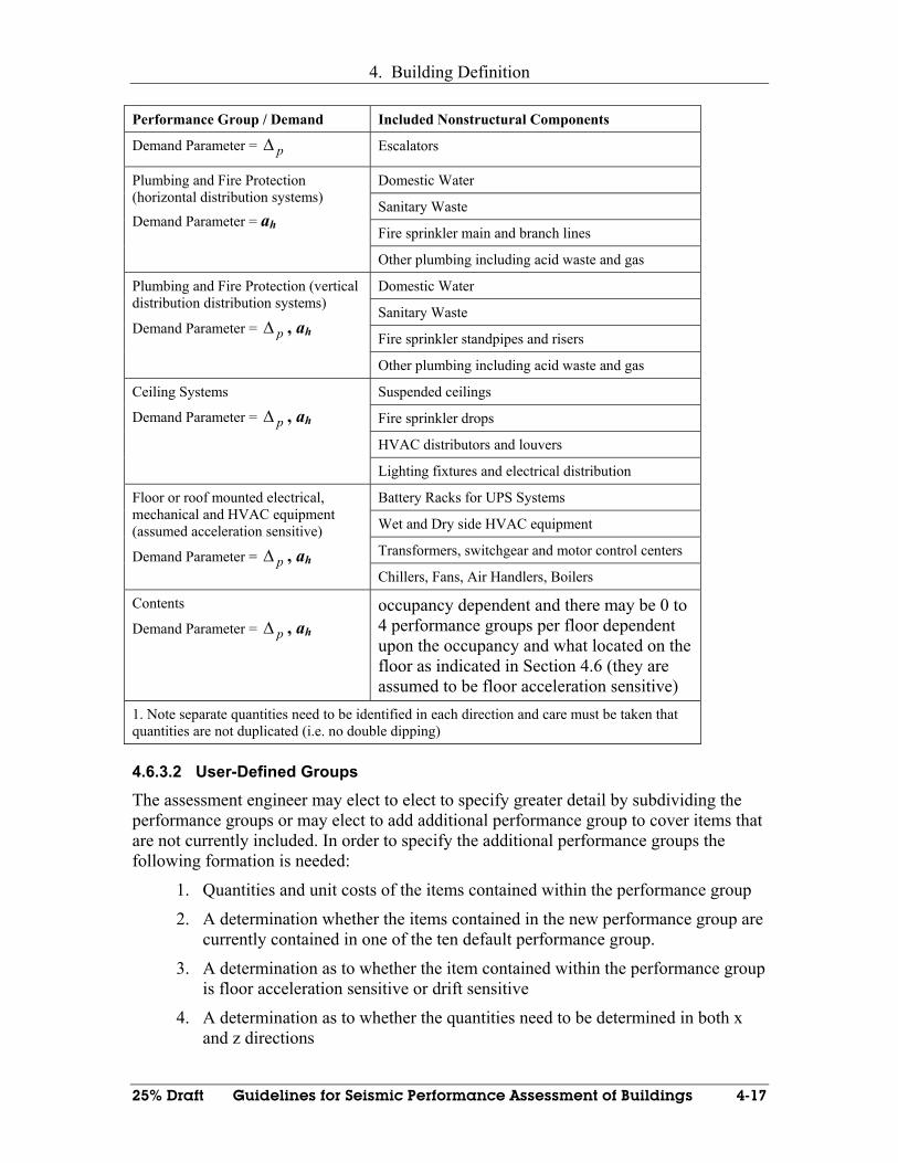
4. Building Definition
25% Draft Guidelines for Seismic Performance Assessment of Buildings 4-17
Performance Group / Demand Included Nonstructural Components
Demand Parameter = p∆ Escalators
Domestic Water
Sanitary Waste
Fire sprinkler main and branch lines
Plumbing and Fire Protection (horizontal distribution systems)
Demand Parameter = ah
Other plumbing including acid waste and gas
Domestic Water
Sanitary Waste
Fire sprinkler standpipes and risers
Plumbing and Fire Protection (vertical distribution distribution systems)
Demand Parameter = p∆ , ah
Other plumbing including acid waste and gas
Suspended ceilings
Fire sprinkler drops
HVAC distributors and louvers
Ceiling Systems
Demand Parameter = p∆ , ah
Lighting fixtures and electrical distribution
Battery Racks for UPS Systems
Wet and Dry side HVAC equipment
Transformers, switchgear and motor control centers
Floor or roof mounted electrical, mechanical and HVAC equipment (assumed acceleration sensitive)
Demand Parameter = p∆ , ah Chillers, Fans, Air Handlers, Boilers
Contents
Demand Parameter = p∆ , ah occupancy dependent and there may be 0 to 4 performance groups per floor dependent upon the occupancy and what located on the floor as indicated in Section 4.6 (they are assumed to be floor acceleration sensitive)
1. Note separate quantities need to be identified in each direction and care must be taken that quantities are not duplicated (i.e. no double dipping)
4.6.3.2 User-Defined Groups
The assessment engineer may elect to elect to specify greater detail by subdividing the performance groups or may elect to add additional performance group to cover items that are not currently included. In order to specify the additional performance groups the following formation is needed:
1. Quantities and unit costs of the items contained within the performance group
2. A determination whether the items contained in the new performance group are currently contained in one of the ten default performance group.
3. A determination as to whether the item contained within the performance group is floor acceleration sensitive or drift sensitive
4. A determination as to whether the quantities need to be determined in both x and z directions

4. Building Definition
4-18 Guidelines for Seismic Performance Assessment of Buildings 25% Draft
5. Fragility functions for the performance group developed in accordance with Appendix C that can be related to damage states and loss functions for use in the performance assessment process. Development of these functions should include a review by qualified experts.

25% Draft Guidelines for Seismic Performance Assessment of Buildings 5-1
5 Ground Shaking Hazards
5.1 Introduction This chapter presents alternate representations of earthquake ground motion for building analysis and performance assessment. Section 5.2 introduces the three alternative characterizations of ground shaking used for intensity-based, scenario-based and time-based assessments, respectively. General procedures for characterizing ground motion for scenario- and time-based performance assessments are described in Section 5.3. A summary presentation on Probabilistic Seismic Hazard Assessment (PSHA), used for the time-based characterization of Section 5.2.4, is presented in Section 5.4. Spectral adjustments to account for the effects of soil-foundation-structure interaction are presented in Section 5.5. Procedures to select and scale earthquake ground motions for nonlinear dynamic response analysis are presented in Section 5.6.
5.2 Characterization of Ground Shaking
5.2.1 Introduction This section introduces the method of characterizing earthquake-induced ground shaking for each of the three types of performance assessment, namely, a) intensity-based, b) scenario-based, and c) time-based. Each of these types of performance assessment requires a somewhat different way of characterizing ground shaking. These procedures are described in more detail in Sections 5.2.2 through 5.2.4, respectively.
5.2.2 Intensity-based assessment Intensity-based assessments of building performance require the specification and quantification of the ground shaking at the intensity for which the assessment is to be performed. Intensity is defined by a 5%-damped, elastic horizontal acceleration response spectrum that is consistent with the characteristics of the site on which the building is constructed. If vertical ground shaking is important to a building’s performance, the horizontal spectrum should be coupled with an appropriate vertical acceleration response spectrum. The ratio of the vertical to horizontal ground shaking spectral ordinates can be estimated using the procedures set forth in Section 5.3.2.
Earthquake acceleration histories (ground motions) used for nonlinear dynamic response analysis should be amplitude scaled to the target acceleration response spectrum. Information on the selection and number of earthquake ground motions required for response analysis, and procedures for scaling the ground motions are presented in Section 5.6.
5.2.3 Scenario-based assessments Seismic source and location data are needed for scenario-based assessments of building performance. Performance is computed for earthquake ground shaking associated with

5. Ground Shaking Hazards
5-2 Guidelines for Seismic Performance Assessment of Buildings 25% Draft
one or more combinations of Moment magnitude and site-to-source distances (e.g., 7WM earthquake shaking from a source 13 km from the building site).
If the [M, r] scenario selected is a near-fault event, that is the building site is within 20 km of the presumed zone of fault rupture and the magnitude is Mw 6.5 or larger, fault directivity effects must be considered by specifying that the scenario event has a) forward directivity (rupture towards the site), b) reverse directivity (rupture away from the site), c) null directivity, or d) unspecified directivity (random direction of rupture). Section 5.4.4 provides additional guidance on fault directivity.
The median and dispersion of the ground shaking intensity parameter obtained from the hazard curve is used to form a scenario hazard curve that indicates the conditional probability of exceeding given intensities of shaking, given that the scenario earthquake occurs. These hazard curves can be conveniently developed by assuming that the probabilistic distribution for the intensity is lognormally distributed. Figure 5-1 presents such a scenario-based hazard curve, constructed assuming a lognormal distribution.
0.01
0.1
1
0.01 0.1 1 10
Spectral Response Accel. at 1 second Sa-1
Con
ditio
nal P
roba
bilit
y of
Exc
eedi
ng S a
for a
G
iven
M, R
0.01
0.1
1
0.01 0.1 1 10
Spectral Response Accel. at 1 second Sa-1
Con
ditio
nal P
roba
bilit
y of
Exc
eedi
ng S a
for a
G
iven
M, R
Figure 5-1, Scenario-based hazard function A minimum of four annual probabilities of exceedance, evenly distributed across the logarithm of the conditional probability of exceedance in the range of 1.0 to 0.01, is used for scenario-based assessments. Eight annual probabilities of exceedance are identified in Figure 5-1 as horizontal blue stripes on the hazard curve. Each of the selected annual probabilities of exceedance defines an intensity band, with a mean value of intensity and a conditional probability of occurrence, given the scenario event. An intensity-based performance assessment is performed at each of these mean intensity levels. The expected value of the scenario performance (e.g., direct loss, downtime, casualties) is then computed as the sum of the intensity-based assessment at the mean intensity level for each band, factored by the conditional probability of occurrence of that intensity, as obtained from the intensity band on the hazard curve.
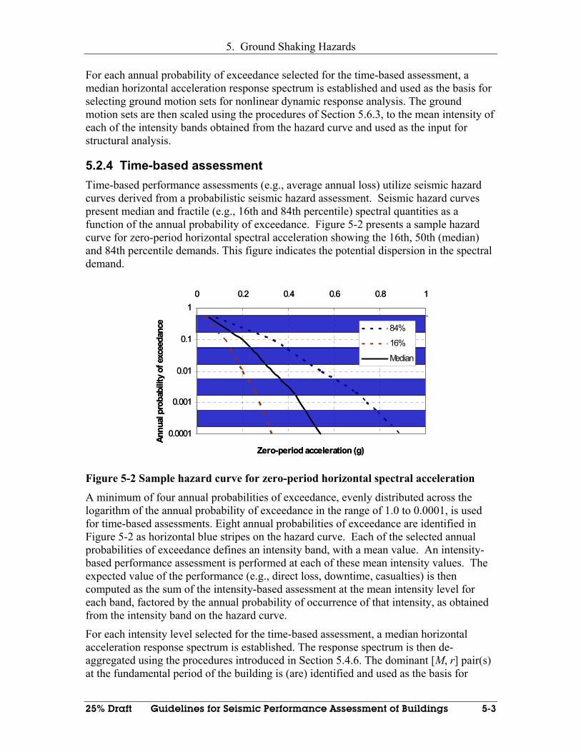
5. Ground Shaking Hazards
25% Draft Guidelines for Seismic Performance Assessment of Buildings 5-3
For each annual probability of exceedance selected for the time-based assessment, a median horizontal acceleration response spectrum is established and used as the basis for selecting ground motion sets for nonlinear dynamic response analysis. The ground motion sets are then scaled using the procedures of Section 5.6.3, to the mean intensity of each of the intensity bands obtained from the hazard curve and used as the input for structural analysis.
5.2.4 Time-based assessment Time-based performance assessments (e.g., average annual loss) utilize seismic hazard curves derived from a probabilistic seismic hazard assessment. Seismic hazard curves present median and fractile (e.g., 16th and 84th percentile) spectral quantities as a function of the annual probability of exceedance. Figure 5-2 presents a sample hazard curve for zero-period horizontal spectral acceleration showing the 16th, 50th (median) and 84th percentile demands. This figure indicates the potential dispersion in the spectral demand.
0.0001
0.001
0.01
0.1
10 0.2 0.4 0.6 0.8 1
Zero-period acceleration (g)
Annu
al p
roba
bilit
y of
exc
eeda
nce
84%
16%
Median
0.0001
0.001
0.01
0.1
10 0.2 0.4 0.6 0.8 1
Zero-period acceleration (g)
Annu
al p
roba
bilit
y of
exc
eeda
nce
84%
16%
Median
Figure 5-2 Sample hazard curve for zero-period horizontal spectral acceleration
A minimum of four annual probabilities of exceedance, evenly distributed across the logarithm of the annual probability of exceedance in the range of 1.0 to 0.0001, is used for time-based assessments. Eight annual probabilities of exceedance are identified in Figure 5-2 as horizontal blue stripes on the hazard curve. Each of the selected annual probabilities of exceedance defines an intensity band, with a mean value. An intensity-based performance assessment is performed at each of these mean intensity values. The expected value of the performance (e.g., direct loss, downtime, casualties) is then computed as the sum of the intensity-based assessment at the mean intensity level for each band, factored by the annual probability of occurrence of that intensity, as obtained from the intensity band on the hazard curve.
For each intensity level selected for the time-based assessment, a median horizontal acceleration response spectrum is established. The response spectrum is then de-aggregated using the procedures introduced in Section 5.4.6. The dominant [M, r] pair(s) at the fundamental period of the building is (are) identified and used as the basis for

5. Ground Shaking Hazards
5-4 Guidelines for Seismic Performance Assessment of Buildings 25% Draft
selecting ground motion sets for nonlinear dynamic response analysis. The ground motion sets are then scaled using the procedures of Section 5.6.3, to the mean intensity of each of the intensity bands obtained from the hazard curve and used as the input for structural analysis.
5.3 General Procedures for Ground Shaking Hazard Assessment
5.3.1 Horizontal shaking spectra Ground motions, represented by response spectra and parameters associated with those spectra, can be determined in accordance with the general procedures of this section except that the site specific procedures of Section 5.4 should be used for class F sites (see Section 5.3.3.1) and for sites outside the conterminous United States.
In this section, spectral acceleration parameters are coefficients corresponding to horizontal spectral response accelerations in units of g, the acceleration due to gravity, and all spectra and associated ground-motion response parameters are computed for 5% of critical damping.
Mapped ground shaking parameters may be obtained from national seismic hazard data prepared by the United States Geological Survey (USSG) at www.usgs.gov. The global coordinates of the building site in latitude and longitude (see Section 4.3.2) are needed to access the data.
The USGS website presents gridded values of peak horizontal ground (zero-period) acceleration, 0.2-second period horizontal spectral acceleration, sS , and 1.0-second period horizontal spectral acceleration, 1S , for 10% and 2% probabilities of exceedance in 50 years (corresponding to annual recurrence rates of approximately 0.002 and 0.0004, respectively), referenced by latitude and longitude. The reported ground-motion values are calculated for firm rock sites (approximately Class B per Section 5.3.3.1), which correspond to a shear-wave velocity of 760 m/sec in the top 30 m of the soil column. The reported values must be modified for soil sites characterized by different shear wave velocities in the upper 30 m. Ground-motion values for the 48 conterminous states have been calculated for a grid spacing of 0.05 degrees; interpolated values are typically calculated using the four surrounding corner points.
For sites with other than Class B soils, the short- ( sS ) and long-period ( 1S ) spectral accelerations at any return period must be adjusted for local site conditions (site class) using equations 5.1 and 5.2, respectively.
ss a sS F S= (5-1)
1 1s vS F S= (5-2)
where aF and vF are defined in Tables 5-1 and 5-2, respectively.
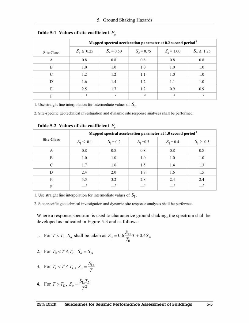
5. Ground Shaking Hazards
25% Draft Guidelines for Seismic Performance Assessment of Buildings 5-5
Table 5-1 Values of site coefficient aF
Mapped spectral acceleration parameter at 0.2 second period 1
Site Class sS ≤ 0.25 sS = 0.50 sS = 0.75 sS = 1.00 sS ≥ 1.25
A 0.8 0.8 0.8 0.8 0.8
B 1.0 1.0 1.0 1.0 1.0
C 1.2 1.2 1.1 1.0 1.0
D 1.6 1.4 1.2 1.1 1.0
E 2.5 1.7 1.2 0.9 0.9
F ___2 ___2 ___2 ___2 ___2
1. Use straight line interpolation for intermediate values of sS .
2. Site-specific geotechnical investigation and dynamic site response analyses shall be performed.
Table 5-2 Values of site coefficient vF
Mapped spectral acceleration parameter at 1.0 second period 1 Site Class
1S ≤ 0.1 1S = 0.2 1S =0.3 1S = 0.4 1S ≥ 0.5
A 0.8 0.8 0.8 0.8 0.8
B 1.0 1.0 1.0 1.0 1.0
C 1.7 1.6 1.5 1.4 1.3
D 2.4 2.0 1.8 1.6 1.5
E 3.5 3.2 2.8 2.4 2.4
F ___2 ___2 ___2 ___2 ___2
1. Use straight line interpolation for intermediate values of 1S .
2. Site-specific geotechnical investigation and dynamic site response analyses shall be performed.
Where a response spectrum is used to characterize ground shaking, the spectrum shall be developed as indicated in Figure 5-3 and as follows:
1. For 0T T< aS shall be taken as 0
0.6 0.4ssa ss
SS T ST
= +
2. For 0 sT T T< ≤ , a ssS S=
3. For s LT T T< ≤ , 1sa
SST
=
4. For LT T> , 12
s La
S TST
=
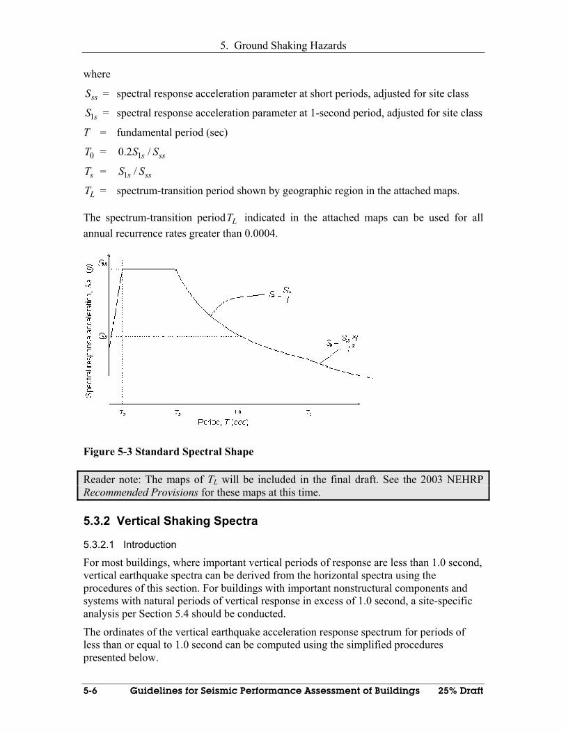
5. Ground Shaking Hazards
5-6 Guidelines for Seismic Performance Assessment of Buildings 25% Draft
where
ssS = spectral response acceleration parameter at short periods, adjusted for site class
1sS = spectral response acceleration parameter at 1-second period, adjusted for site class
T = fundamental period (sec)
0T = 10.2 /s ssS S
sT = 1 /s ssS S
LT = spectrum-transition period shown by geographic region in the attached maps.
The spectrum-transition period LT indicated in the attached maps can be used for all annual recurrence rates greater than 0.0004.
Figure 5-3 Standard Spectral Shape
Reader note: The maps of TL will be included in the final draft. See the 2003 NEHRP Recommended Provisions for these maps at this time.
5.3.2 Vertical Shaking Spectra
5.3.2.1 Introduction
For most buildings, where important vertical periods of response are less than 1.0 second, vertical earthquake spectra can be derived from the horizontal spectra using the procedures of this section. For buildings with important nonstructural components and systems with natural periods of vertical response in excess of 1.0 second, a site-specific analysis per Section 5.4 should be conducted.
The ordinates of the vertical earthquake acceleration response spectrum for periods of less than or equal to 1.0 second can be computed using the simplified procedures presented below.

5. Ground Shaking Hazards
25% Draft Guidelines for Seismic Performance Assessment of Buildings 5-7
5.3.2.2 General procedure for Site Classes A, B and C
For structural periods less than or equal to 1.0 second, the vertical response spectrum can be constructed by scaling the corresponding ordinates of the horizontal response spectrum, aS , as follows.
For periods less than or equal to 0.1 second, the vertical spectral acceleration, vS , can be taken as
v aS S= (5-3)
For periods between 0.1 and 0.3 second, the vertical spectral acceleration, vS , can be taken as
(1 1.048[log( ) 1])v aS T S= − + (5-4)
For periods between 0.3 and 1.0 second, the vertical spectral acceleration, vS , can be taken as
0.5v aS S= (5-5)
5.3.2.3 General procedure for Site Classes D and E
For structural periods less than or equal to 1.0 second, the vertical response spectrum can be constructed by scaling the corresponding ordinates of the horizontal response spectrum, aS , as follows.
For periods less than or equal to 0.1 second, the vertical spectral acceleration, vS , can be taken as
v aS Sη= (5-6)
For periods between 0.1 and 0.3 second, the vertical spectral acceleration, vS , can be taken as
( 2.1( 0.5)[log( ) 1])v aS T Sη η= − − + (5-7)
For periods between 0.3 and 1.0 second, the vertical spectral acceleration, vS , can be taken as
0.5v aS S= (5-8)
In equations (5-6) and (5-7), factor η can be taken as 1.0 for 0.5sS g≤ ; 1.5 for 1.5sS g≤ ; and (1 0.5( 0.5))sS+ − for 0.5 1.5sg S g≤ ≤ .

5. Ground Shaking Hazards
5-8 Guidelines for Seismic Performance Assessment of Buildings 25% Draft
5.3.3 Site class definition and classification
5.3.3.1 Site class definition
Site classes, A through F, are as defined in Table 5.3.
Table 5-3 Site class definitions
Class Description
A Hard rock with measured shear wave velocity, sν > 5,000 ft/sec (1500 m/s).
B Rock with 2,500 ft/sec < sν ≤ 5,000 ft/sec (760 m/s < sν ≤ 1500 m/s).
C Very dense soil and soft rock with 1,200 ft/sec < sν ≤ 2,500 ft/sec (360 m/s < sν ≤ 760 m/s)
or with either N > 50 or us > 2,000 psf (100 kPa).
D Stiff soil with 600 ft/sec sν≤ ≤ 1,200 ft/sec (180 m/s sν≤ ≤ 360 m/s) or with either 15
N≤ ≤ 50 or 1,000 psf us≤ ≤ 2,000 psf (50 kPa us≤ ≤ 100 kPa).
E A soil profile with sν < 600 ft/sec (180 m/s) or with either N < 15, us < 1,000 psf, or any profile with more than 10 ft (3 m) of soft clay defined as soil with PI > 20, w ≥ 40 percent, and us < 500 psf (25 kPa).
F
Soils requiring site-specific evaluations: a) soils vulnerable to potential failure or collapse under seismic loading such as liquefiable soils, quick and highly sensitive clays, collapsible weakly cemented soils; b) peat and/or highly organic clays (H > 10 ft [3 m] of peat and/or highly organic clay, where H = thickness of soil); c) very high plasticity clays (H > 25 ft [8 m] with PI > 75; and d) very thick, soft/medium stiff clays (H > 120 ft [36 m]) with us < 1,000 psf (50 kPa).
The parameters used to define the Site Class are based on the upper 100 ft (30 m) of the site soil profile. Profiles containing distinctly different soil and rock layers are subdivided into those layers designated by a number that ranges from 1 to n at the bottom, where there are a total of n distinct layers in the upper 100 ft (30 m). The following procedures are used to compute average (weighted) soil properties (shear wave velocity, penetration resistance and undrained shear strength) for the purpose of site classification.
The weighted shear wave velocity, sv , is calculated as
1
1
n
ii
s ni
sii
dv
dv
=
=
=∑
∑ (5-9)
where siν is the shear wave velocity in ft/sec (m/s); and id is the thickness of any layer (between 0 and 100 ft [30 m]) and the sum of the n values of id is 100 ft (30 m).
5. Ground Shaking Hazards
25% Draft Guidelines for Seismic Performance Assessment of Buildings 5-9
The weighted penetration resistance, N , is calculated using equation 5-10.
1
1
n
iin
i
ii
dN
dN
=
=
=∑
∑ (5-10)
where iN is the Standard Penetration Resistance determined in accordance with ASTM D 1586, as directly measured in the field without corrections, and shall not be taken greater than 100 blows/ft; where refusal is met for a rock layer, Ni is taken as 100 blows/ft. In this equation, iN and id apply to cohesionless soil, cohesive soil and rock layers.
1
sch m
i
ii
dNdN=
=
∑ (5-11)
where iN and id in equation (5-10) are for cohesionless soil layers only, sd is the total thickness of cohesionless soil layers in the top 100 ft (30 m) and the sum of the n values of id is 100 ft (30 m).
The average undrained shear strength, us , in psf (kPa), is calculated using equation (5-12).
1
cu k
i
uii
dsds=
=
∑ (5-12)
where the undrained shear strength shall be determined in accordance with ASTM D 2166 or D 2850, and is not taken greater than 5,000 psf (250 kPa); and cd is the total thickness of cohesive soil layers in the top 100 ft (30 m).
For other computations associated with site class classification, PI is the plasticity index, determined in accordance with ASTM D 4318, and w is the moisture content in percent, determined in accordance with ASTM D 2216.
5.3.3.2 Site classification
The following simplified procedures can be used to classify the class of soils beneath a building site.
Assign Site Classes A and B based on the shear wave velocity for rock. Where hard rock conditions are known to be continuous to a depth of 100 ft (30 m), surfacial shear wave velocity measurements may be extrapolated to assess sν . Do not use Site classes A and B where there is more than 10 ft (3 m) of soil between the rock surface and the bottom of the spread footing or mat foundation.

5. Ground Shaking Hazards
5-10 Guidelines for Seismic Performance Assessment of Buildings 25% Draft
If any of the four categories of Site Class F apply [a) through d) in Table 5.3], a site-specific evaluation is required and the procedures of this section do not apply.
Classify the site as Site Class E if the total thickness of soft clay > 10 ft (3 m), where a soft clay layer is defined by: us < 500 psf (25 kPa), w ≥ 40 percent, and PI > 20.
Site classes C, D and E can be assigned using one of the average or weighted measures presented in Table 5.4 and equations (5.9) through (5.11), namely,
sν for the top 100 ft (30 m) ( sν method)
N for the top 100 ft (30 m) ( N method)
chN for cohesionless soil layers (PI < 20) in the top 100 ft (30 m) and the average
us for cohesive soil layers (PI > 20) in the top 100 ft (30 m) ( us method).
Table 5-4 Classification for site classes C, D and E
Site Class sν N or chN us 1
C > 1,200 to 2,500 fps
(360 to 760 m/s) > 50
> 2,000 ( > 100 kPa)
D 600 to 1,200 fps (180 to 360 m/s)
15 to 50 1,000 to 2,000 psf (50 to 100 kPa)
E < 600 fps
( < 180 m/s) < 15
< 1,000 psf ( < 50 kPa)
1. If the us method is used and the chN and us criteria differ, select the category with the softer soils.
5.3.4 Adjustment for other exceedance probabilities Acceleration response spectra for earthquake hazard levels corresponding to probabilities of exceedance between 2% in 50 years and 50% in 50 years can be derived using the following procedures.
For probabilities of exceedance, EYP , between 2% in 50 years and 10% in 50 years (i.e., return period between 475 and 2,475 years), where the Maximum Considered Earthquake (MCE) mapped short-period response acceleration parameter, sS , is less than 1.5 g, the modified mapped short-period ( sS ) and 1.0-second ( 1S ) response acceleration parameters can be determined using equation (5-13).
10 /50 MCE 10/50ln( ) ln( [ln( ) ln( )][0.606ln( ) 3.73]i i i i RS S S S P= + + − − (5-13)
where ln( )iS is the natural logarithm of the spectral acceleration parameter ( i s= for short period and 1.0i = for 1-second period) at the desired probability of exceedance;
10/ 50ln( )iS is the natural logarithm of the spectral acceleration parameter ( i s= for short period and 1.0i = for 1-second period) at a 10% probability of exceedance in 50 years;
MCEln( )iS is the natural logarithm of the spectral acceleration parameter ( i s= for short
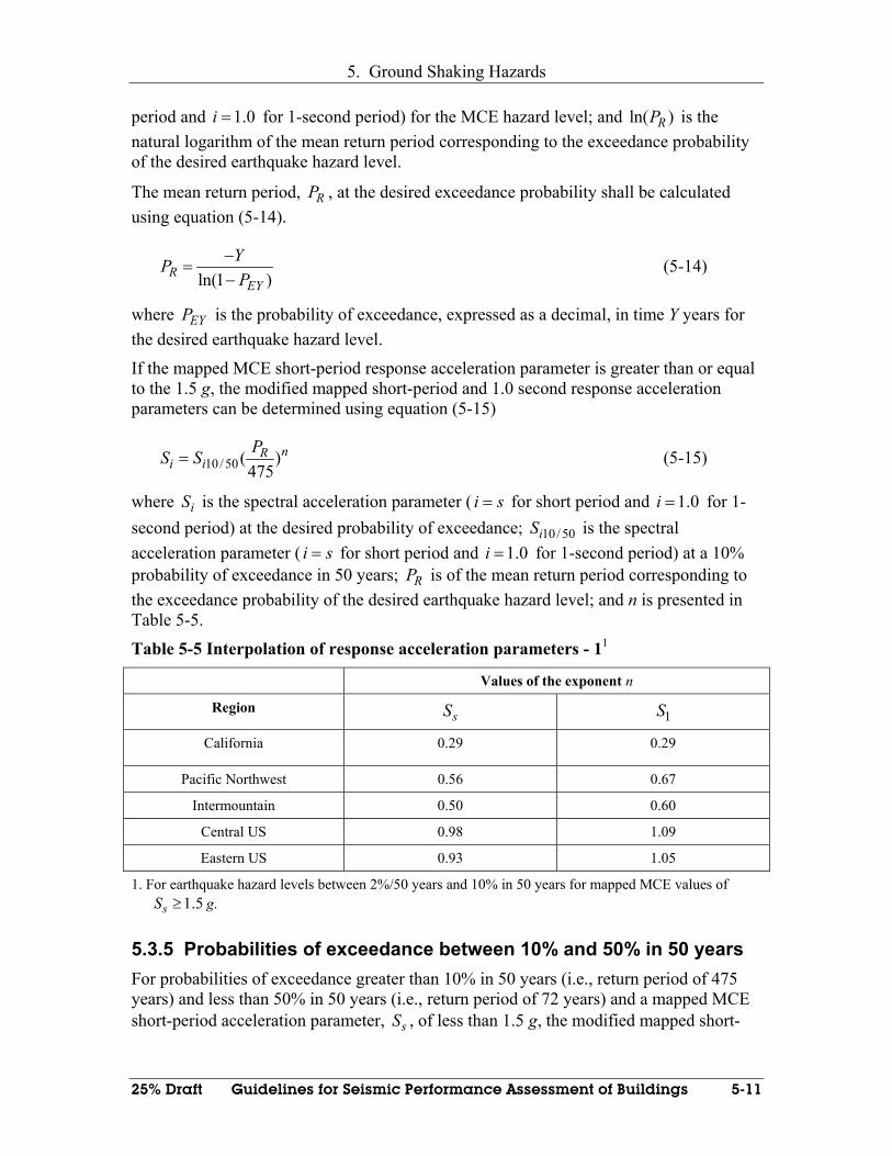
5. Ground Shaking Hazards
25% Draft Guidelines for Seismic Performance Assessment of Buildings 5-11
period and 1.0i = for 1-second period) for the MCE hazard level; and ln( )RP is the natural logarithm of the mean return period corresponding to the exceedance probability of the desired earthquake hazard level.
The mean return period, RP , at the desired exceedance probability shall be calculated using equation (5-14).
ln(1 )REY
YPP
−=
− (5-14)
where EYP is the probability of exceedance, expressed as a decimal, in time Y years for the desired earthquake hazard level.
If the mapped MCE short-period response acceleration parameter is greater than or equal to the 1.5 g, the modified mapped short-period and 1.0 second response acceleration parameters can be determined using equation (5-15)
10/ 50( )475
nRi i
PS S= (5-15)
where iS is the spectral acceleration parameter ( i s= for short period and 1.0i = for 1-second period) at the desired probability of exceedance; 10/ 50iS is the spectral acceleration parameter ( i s= for short period and 1.0i = for 1-second period) at a 10% probability of exceedance in 50 years; RP is of the mean return period corresponding to the exceedance probability of the desired earthquake hazard level; and n is presented in Table 5-5.
Table 5-5 Interpolation of response acceleration parameters - 11
Values of the exponent n
Region sS 1S
California 0.29 0.29
Pacific Northwest 0.56 0.67
Intermountain 0.50 0.60
Central US 0.98 1.09
Eastern US 0.93 1.05
1. For earthquake hazard levels between 2%/50 years and 10% in 50 years for mapped MCE values of 1.5sS ≥ g.
5.3.5 Probabilities of exceedance between 10% and 50% in 50 years For probabilities of exceedance greater than 10% in 50 years (i.e., return period of 475 years) and less than 50% in 50 years (i.e., return period of 72 years) and a mapped MCE short-period acceleration parameter, sS , of less than 1.5 g, the modified mapped short-

5. Ground Shaking Hazards
5-12 Guidelines for Seismic Performance Assessment of Buildings 25% Draft
period and 1.0 second response acceleration parameters can be determined using equation (5-15), where the exponent n is given in Table 5-6.
Table 5-6 Interpolation of response acceleration parameters - 21
Values of the exponent n
Region sS 1S
California 0.44 0.44
Pacific Northwest 0.54 0.59
Intermountain 0.54 0.59
Central US 0.77 0.80
Eastern US 0.77 0.80
1. For earthquake hazard levels greater than 10% in 50 years and mapped MCE values of 1.5sS < g.
For probabilities of exceedance between 10% and 50% in 50 years and a mapped MCE short-period acceleration parameter, sS , of equal to or greater than 1.5 g, the modified mapped short-period and 1.0 second response acceleration parameters can be determined using equation (5-20), where the exponent n is given in Table 5-7.
Table 5-7 Interpolation of response acceleration parameters - 31
Values of the exponent n
Region sS 1S
California 0.44 0.44
Pacific Northwest 0.89 0.96
Intermountain 0.54 0.59
Central US 0.89 0.89
Eastern US 1.25 1.25
1. For earthquake hazard levels greater than 10% in 50 years and mapped MCE values of 1.5sS ≥ g.
For other probabilities of exceedance, a probabilistic seismic hazard analysis should be conducted. The use of interpolation functions requires that the response spectrum corresponding to a 10% probability of exceedance in 50 years be derived. Information provided at www.usgs.gov and presented in Section 5.3.1 can be used for this purpose.
5. Ground Shaking Hazards
25% Draft Guidelines for Seismic Performance Assessment of Buildings 5-13
5.4 Site-Specific Procedures for Ground Shaking Hazard Assessment
5.4.1 Introduction Site-specific characterization of the ground shaking associated with different probabilities of exceedance can be used for performance assessment on any site and must be used on Site Class F sites. Such characterizations are routinely performed using Probabilistic Seismic Hazard Assessment. Section 5.4.2 provides introductory information on Probabilistic Seismic Hazard Assessment.
Attenuation relationships, described earlier in Section 5.2.3, are key components of a probabilistic seismic hazard assessment and are used to characterize the hazard for scenario-based performance assessments. Introductory information on attenuation relationships is provided in Section 5.4.3. Rupture directivity can substantially affect the amplitude and duration of earthquake shaking in the near-fault region. Section 5.4.4 introduces guidance for the consideration of rupture directivity. Section 5.4.5 provides summary information on the inclusion of local soil (site) effects in attenuation relationships.
Sets of earthquake ground motions are used for nonlinear dynamic response analysis. Procedures for selecting appropriate sets of motions, based on de-aggregation of seismic hazard curves, are presented in Section 5.4.6.
5.4.2 Probabilistic seismic hazard assessment The standard products of a Probabilistic Seismic Hazard Assessment include hazard curves similar to those presented in Figure 5-2 for a range of periods (frequencies); response spectra corresponding to specific annual probabilities of exceedance, and de-aggregations of response spectra at selected periods into [M, r] pairs. The key steps in a standard PSHA are
• Identify and characterize (geometry and potential [ WM ]) all earthquake sources capable of generating significant shaking (say 4.5WM ≥ ) at the building site. Develop the probability distribution of rupture locations within each source. Combine this distribution with the source geometry to obtain the probability distribution of source-to-site distance for each source.
• Develop a seismicity or temporal distribution of earthquake occurrence for each source using a recurrence relationship.
• Using predictive (attenuation) relationships, determine the ground motion produced at the building site (including the uncertainty) by earthquakes of any possible size or magnitude occurring at any possible point in each source zone. See Section 5.4.3 for more details.
• Combine the uncertainties in earthquake location, size, and ground motion prediction to obtain the probability that the chosen ground motion parameter (e.g., peak horizontal ground acceleration, spectral acceleration at a specified frequency) will be exceeded in a particular time period (e.g., 10% in 50 years).

5. Ground Shaking Hazards
5-14 Guidelines for Seismic Performance Assessment of Buildings 25% Draft
Kramer (1996) and McGuire (2004) provide much information on this process for the interested reader.
5.4.3 Attenuation relationships Attenuation relationships relate ground motion parameters to the magnitude of an earthquake and the distance away from the fault rupture. Relationships have been established for many ground motion parameters including peak horizontal and vertical ground acceleration, velocity, displacement and corresponding spectral terms. In these Guidelines, attenuation relationships are used to characterize shaking for scenario-based assessments and as part of a probabilistic seismic hazard assessment for time-based assessments.
Attenuation relationships are developed by statistical evaluation of large sets of ground motion data. Relationships have been developed for different regions of the United States (and other countries) and different fault types (i.e., strike-slip, dip-slip and subduction). These relationships are only as good as the dataset from which the relationships were derived; the greater the size of the data set, the more robust the relationship. A set of attenuation relationships, that plot peak horizontal acceleration versus distance in a log-log scale is presented below in Figure 5-4 (Abrahamson and Shedlock, 1997).
In its most basic form, the attenuation relationship can be described by an equation of the form:
1 2 3 4ln lnY c c M c R c R ε= + − − + (5-16)
where lnY is the natural logarithm of the strong-motion parameter of interest (e.g., peak ground acceleration, spectral horizontal acceleration), M is the earthquake magnitude, R is the source-to-site distance or a term characterizing this distance, and ε is the standard error term with a mean of zero and a standard deviation of lnYσ , which is the dispersion for the attenuation relationship. The term 2c M is consistent with the definition of earthquake magnitude (the source) as a logarithmic measure of the amplitude of the ground motion. The term 3 lnc R− (the path) is consistent with the geometric spread of the seismic wave front as it propagates from the source. The value of 3c will vary with distance depending on the seismic wave type (body wave, surface wave, etc). The term
4c R− is consistent with the anelastic attenuation of seismic waves caused by material damping (treating soil as a viscoelastic material) and scattering (a result of reflections and refractions of seismic waves due to the presence of heterogeneities and discontinuities in the earth’s crust, causing multiple seismic waves to arrive at a site from different paths of differing lengths). Typical attenuation relationships are more complicated than the basic equation given above. Additional terms are needed to account for other effects including near-source directivity, faulting mechanism (strike slip, reverse and normal), site conditions (different relationships), and hanging wall/footwall location of the site.

5. Ground Shaking Hazards
25% Draft Guidelines for Seismic Performance Assessment of Buildings 5-15
Figure 5-4 Sample attenuation relationships (Abrahamson and Shedlock, 1997)
5.4.4 Near-Fault Rupture Directivity Rupture directivity causes spatial variations in the amplitude and duration of ground motions within 20 km of major active faults. Propagation of rupture towards a site produces larger amplitudes of shaking transverse to the direction of fault rupture at periods longer than 0.6 second and shorter strong-motion durations than for average directivity conditions. On such sites, ground shaking parallel to the direction of fault rupture, tend to be significantly reduced from those transverse to the fault rupture direction, an effect known as directionality. A characterization of the ground shaking hazard at a site within 20 km of a major active fault should address rupture directivity and shaking directionality.
5.4.5 Characterization of site effects In probabilistic seismic hazard assessment, site effects are traditionally captured either through use of attenuation relationships that are specific to the particular site class of interest or by making modifications to the intensity of motion obtained from the attenuation relationships to account for site class effects.
5.4.6 Deaggregation of the seismic hazard curves The probabilistic seismic hazard analysis procedures described in Section 5.4.2 permit the calculation of annual rates of exceedance at a particular site based on aggregating the risks from all possible source zones. The rate of exceedance computed in the probabilistic seismic hazard analysis is therefore not associated with any particular earthquake magnitude M or distance r.
The three component sets of earthquake histories that are used for detailed-level performance assessments using nonlinear dynamic response analysis should be representative of the corresponding hazard. De-aggregation of the hazard, in terms of [M,

5. Ground Shaking Hazards
5-16 Guidelines for Seismic Performance Assessment of Buildings 25% Draft
r] pairs, as a function of period, can be used to guide the selection of appropriate earthquake histories.
For a given building site and hazard curve, the combinations of magnitude, distance and source that contribute most to the hazard curve can be established. This process is termed de-aggregation (or disaggregation). Hazard deaggregation requires that the mean annual rate of exceedance be expressed as a function of magnitude and distance.
Detailed information on the deaggregation of seismic hazard curves is provided in McGuire (2004). The U.S.G.S provides data on deaggregated hazard for sites throughout the continental Untied States, on their website. Sample results for horizontal spectral acceleration at periods of 0.2 second and 1.0 second for a site in San Francisco, for a 2% probability of exceedance in 50 years, are shown in Figure 5-5 below (www.usgs.gov).
a. 0.2 second b. 1.0 second
Figure 5-5 Sample de-aggregation of a seismic hazard curve (www.usgs.gov)
5.5 Spectral Adjustment for Soil-Foundation Structure Interaction
Section 6.2.2 presents simplified procedures for accounting for two effects of soil-foundation-structure interaction, namely, kinematic interaction and foundation damping. Each effect can substantially modify the free-field motions, leading to significant reductions in spectral demands on the structure, especially in the short period range.
For buildings with fundamental periods of vibration of 0.5 seconds or less, five-percent damped elastic response spectra developed using either the procedures of Section 5.3 or Section 5.4, should be modified as described in Section 6.2.2 to account for the effects of soil foundation structure interaction. Earthquake ground motions generated for nonlinear dynamic response analysis of such structures, per Section 5.6 should be based on soil foundation structure interaction modified spectra instead of the free-field spectra of Sections 5.3 and 5.4.

5. Ground Shaking Hazards
25% Draft Guidelines for Seismic Performance Assessment of Buildings 5-17
5.6 Generation of Ground Motions for Response-History Analysis
5.6.1 Introduction The detailed-level performance assessment procedures of these Guidelines utilize nonlinear dynamic response analysis, which requires the selection and scaling of earthquake ground motions. This section describes how sets of three-component earthquake ground motions (histories) can be selected and scaled for such analysis.
Section 5.6.2 describes how recorded (unscaled) ground motions are selected. Procedures for scaling ground motions are presented in Section 5.6.3. Guidance on the number of sets of three-component ground motions required for nonlinear dynamic response analysis is presented in Section 5.6.2.
5.6.2 Selection of ground motions Recorded (unscaled) three-component (2 horizontal, 1 vertical) sets of earthquake ground motions must be appropriately scaled and used as the input motion for nonlinear dynamic analysis. Unscaled three-component sets of ground motions are available for download from a number of databases, including:
http://peer.berkeley.edu/smcat/,
http://db.cosmos-eq.org/scripts/default.plx,
http://smdb.crustal.ucsb.edu,
The deaggregation of the seismic hazard curve (see Section 5.4.6) at the selected annual rate of exceedance and period (frequency) of interest, by Moment magnitude, source-to-site distance and source type (e.g., strike-slip, reverse or normal faulting) is the state of practice (e.g, USNRC NUREG RG-1.165 and CR-6728) and can be used to guide the selection of ground motions used for analysis. The earthquake ground motions are then chosen on the basis of the expected value of magnitude and distance given the annual rate of exceedance and the selected structural period. The local geology (e.g., site class per Section 5.3.3) at the site of the building should be used to filter and select the ground motions (i.e., the site geology at which the record was obtained should be similar to that of the building site).
A uniform hazard response spectrum generated by probabilistic seismic hazard analysis for a selected probability of exceedance (say 2%) in a given time period (e.g., 50 years) does not represent the response of a single-degree-of-freedom oscillator of varying frequency to a single ground motion. Rather, deaggregation of a uniform hazard spectrum will generally show that different combinations of magnitude and distance dominate the hazard at different periods, especially if multiple sources are present and the hazard is not dominated by a fault with a large characteristic earthquake. For many sites in the North America, the short-period hazard is dominated by moderate magnitude, short distance earthquakes and the long-period hazard is dominated by large-magnitude, moderate distance earthquakes. In such cases, no single [M, r] pair will suffice as the basis for selecting ground motions for scaling per Section 5.6.3.
5. Ground Shaking Hazards
5-18 Guidelines for Seismic Performance Assessment of Buildings 25% Draft
The performance-assessment and loss-computation procedures presented elsewhere in these Guidelines address structural and nonstructural components and building contents. The displacement response of (and thus damage to) most framing systems in building structures can be tied to the first mode (or degraded first mode) of translational response along each principal axis of the building. Generally, damage to drift sensitive nonstructural components will also be a function of this mode of response. Ground motions selected to estimate deformation, damage and performance of structural components will therefore serve an identical function for drift-sensitive nonstructural components. However, many nonstructural components in buildings are acceleration sensitive and many of these components exhibit short period response (e.g., horizontal piping systems and suspended ceiling systems). Ground motions based on the expected [M, r] pair at the first mode period of the building (e.g., 2 seconds) may have insufficient short-period acceleration demand to assess the likely damage and loss to the acceleration sensitive nonstructural components and building contents.
5.6.3 Ground motion scaling
5.6.3.1 Introduction
This section provides guidance for the scaling of earthquake ground motions, selected using the procedures of Section 5.6.2. Procedures for scaling earthquake ground motions for the case where one [M, r] pair dominates the hazard curve at all periods of interest are presented in Section 5.6.3.3. Procedures for scaling earthquake ground motions for the case where two or three [M, r] pairs characterize the hazard curve at the periods of interest are presented in Section 5.6.3.4. Spectrally matched ground motions should not be used for performance assessment.
The frequencies (periods) of interest assumed in the development of these scaling procedures address the response of both structural and nonstructural components and contents. For structural response, the nominal period range of interest is 0.2T to 1.5T, where T is the elastic period of the structural framing system. Both principal horizontal axes of the building should be considered for this computation and the minimum and maximum values of 0.2T and 1.5T for both axes should be used to define the period range. The value of 0.2T represents an estimate of the second mode period; 1.5T is an estimate of the degraded first mode period (due to damage to the structural frame). A more accurate estimate of the second mode period, based on eigenvalue analysis, could be used in lieu of 0.2T. The period range of interest for the nonstructural components and contents should be established by considering the systems present. Generally, the period range of interest for these components will be .05 seconds to .2 seconds.
5.6.3.2 Ground motion scaling if one [M, r] pair dominates the hazard
If one [M, r] pair dominates the selected uniform hazard spectrum across the period range of interest, denoted herein as min maxT T T≤ ≤ , the following procedure can be used to scale the motions. The procedure will retain randomness in the earthquake shaking. A minimum of twenty sets of three-component earthquake histories should be generated for nonlinear dynamic response analysis.

5. Ground Shaking Hazards
25% Draft Guidelines for Seismic Performance Assessment of Buildings 5-19
Reader note: The minimum number of sets of three component earthquake histories to be used for performance assessment is the subject of a current study. The work completed to date suggests that up to twenty sets of histories might be required for analysis. Updated information will be presented in a later draft of the Guideline.
Scale each pair of horizontal earthquake histories to minimize the sum of the squared error between the uniform hazard spectrum and the geometric mean of the spectral ordinates for the pair of histories at periods of minT , maxT and two equally spaced periods between minT and maxT (e.g., if min 0.30T = second and max 1.5T = seconds, the intermediate periods would be 0.7 and 1.1 seconds.) Statistically test the spectra of the resultant scaled horizontal earthquake histories to ensure that the randomness in the ground motion shaking is preserved.
Reader note: Rules for the consistent scaling of vertical ground motions will be developed before the publication of the next draft of the Guideline.
5.6.3.3 Ground motion scaling if multiple [M, r] pairs dominates the hazard
If multiple [M, r] pairs dominate the selected uniform hazard spectrum across the period range of interest, denoted herein as min maxT T T≤ ≤ , the following procedure can be used to scale the seed motions. Select seven sets of three-component earthquake histories for each [M, r] pair.
Reader note: Procedures to statistically interpret the results of response analysis using ground motions scaled to different period ranges of a spectrum will be developed before the publication of the next draft of the Guideline.


25% Draft Guidelines for Seismic Performance Assessment of Buildings 6-1
6 Response Quantification
6.1 Scope This section describes numerical modeling techniques and analysis procedures for use in building performance assessment. Section 6.2 provides general recommendations for the analysis of structural framing systems, including procedures to account for soil-foundation-structure interaction, procedures for modeling components of structural frames and assembly of those components into models of structural systems, and representations of ground shaking. Procedures for linear static and dynamic nonlinear response analysis are provided in Section 6.3. Demand parameters that should be monitored for structural and nonstructural components (and contents) in buildings are identified in Sections 6.4 and 6.5, respectively.
6.2 General Analysis Requirements
6.2.1 Introduction This section provides guidance on modeling soil-foundation-structure interaction (Section 6.2.2) and modeling of structural components, structural elements and structural systems (Section 6.2.3).
6.2.2 Soil-foundation-structure interaction
6.2.2.1 Introduction
Probablistic seismic hazard analysis, and attenuation relationships used by such analysis produce estimates of ground shaking in the form of uniform hazard spectra that are valid in the free field. However, these free field estimates of ground shaking intensity often overstate the intensity of shaking that is actually experienced by structures. Structures that have below grade levels, and which are deeply embedded in a site, tend to experience reduced levels of ground shaking relative to structures with shallow foundations and little embedment. Structures with relatively large footprints, and rigidly inter-tied foundation systems tend to filter out short period components of free field ground shaking. As structures respond to ground shaking, they radiate energy outward into the surrounding soils, introducing damping. These three behaviors are generally classified as soil-foundation-structure interaction and tend to significantly reduce the effective amplitude of ground shaking response spectra, particularly at short periods. Sections 6.2.2.2 and 6.2.2.3 introduce simplified and rigorous procedures for evaluating these soil-foundation-structure effects, respectively.
6.2.2.2 Simplified soil-foundation-structure-interaction analysis
6.2.2.2.1 General
Simplified procedures for including the effects of soil-foundation-structure interaction, grouped herein under the headings of kinematic interaction and foundation damping, are

6. Response Quantification
6-2 Guidelines for Seismic Performance Assessment of Buildings 25% Draft
introduced in the following subsections. Much additional information is presented in FEMA 440 (FEMA 2005).
Reader note: Additional guidance on procedures to address kinematic interaction and foundation damping for the purpose of nonlinear dynamic response analysis will be presented in a later draft.
6.2.2.2.2 Kinematic interaction
A ratio-of-response-spectra (RRS) factor can be used to reduce the effective amplitude of free field response spectra resulting from kinematic interaction effects. This factor is the ratio of the effective response-spectrum ordinates imposed on the foundation (i.e., the foundation input motion) to the free-field spectral ordinates. Two phenomena should be considered in evaluating the RRS: base-slab averaging and foundation embedment. The reductions in spectral demand due to base-slab averaging and embedment can be appreciable and should be considered for buildings with a fixed-base period of less than 1 second. The effects of base-slab averaging can be ignored if the maximum plan dimension of the building is 100 feet or less and must be neglected for structures on soft clays, site classes E or F. The effects of embedment can be ignored for foundations embedded in rock that conforms to either Site Class A or B per Section 5.3.
The simplified procedure of Chapter 8 of FEMA 440 (FEMA, 2005) can be used for assessment of kinematic interaction. The following information is needed for such an assessment: dominant building period (as measured by % mass participating in the elastic base shear computation), building foundation plan dimension, foundation embedment, peak horizontal ground acceleration, and shear wave velocity. Limitations on the use of the simplified procedure are presented in Section 8 of FEMA 440. Figure 6-1 and 6-2, reproduced here from FEMA-440, indicate the reduction in response spectra (RRS) that can be achieved from these effects.
Figure 6-1 Reduction in Response Spectra, base-slab averaging (kinematic) effects, from FEMA 440.

6. Response Quantification
25% Draft Guidelines for Seismic Performance Assessment of Buildings 6-3
Figure 6-2 Reduction in Response Spectra, foundation embedment effects, from FEMA 440.
6.2.2.2.3 Foundation damping
Damping related to soil-foundation interaction due to hysteretic soil damping and radiation damping can significantly increase the effective damping in a structural frame, thereby reducing the ordinates of a 5% damped acceleration response spectrum, which is generally used as the basis for generating earthquake histories for response-history analysis.
The simplified procedure of FEMA 440 can be used for assessment of foundation damping. Hysteretic damping in the soil should be captured directly through the use of nonlinear soil springs. The following information is needed for such an assessment: dominant (first mode) building period (as measured by % mass participating in the elastic base shear computation), 1T ; first modal mass; building foundation plan dimension; building height; foundation embedment; strain-degraded soil shear modulus and soil Poisson’s ratio. Limitations on the use of the simplified procedure are presented in Section 8 of FEMA 440.
6.2.2.3 Direct soil-foundation-structure-interaction analysis
Soil-foundation-structure interaction can be analyzed directly using the finite-element method and response history analysis techniques, where the soil is discretized with solid finite elements. Full nonlinear analysis is also possible using this method although typical analysis is performed using equivalent linear soil properties. Direct analysis can address the three key effects of soil-foundation-structure interaction (foundation flexibility, kinematic effects, and foundation damping) although solution of the kinematic interaction problem is often difficult without customized finite element codes because typical finite element codes cannot account for wave inclination and wave incoherence effects.

6. Response Quantification
6-4 Guidelines for Seismic Performance Assessment of Buildings 25% Draft
Time-domain analysis will require the development of a two- or three-dimensional numerical model of the soil-foundation-structure system. Stress-strain or constitutive models (linear, nonlinear or equivalent linear) for the soils in the model should be developed based on test data. Appropriate and consistent frequency-dependent stiffness and damping matrices should be developed for the edges or boundaries of the soil in the numerical model. Guidance for modeling the structural components of the framing system and the foundation (assumed herein to be composed of structural components) is provided in Section 6.2.3 and the appendices.
Reader note: Additional guidance on direct soil-foundation-structure interaction including the effect of adjacent buildings, nonlinear modeling of soils, and procedures to develop frequency-dependent stiffness and damping matrices for the edges or boundaries of the soil will be included in a later draft.
6.2.3 Structural system and component modeling
6.2.3.1 Conceptual level models for performance assessment
Linear static analysis of lumped parameter models of buildings per Section 6.3.2 is sufficient for conceptual level performance evaluation and loss computations. Dynamic nonlinear response analysis of lumped parameter models is also permitted per Section 6.3.3.
The base of a lumped parameter model can be assumed to be fixed against translation and rotation. Translational masses shall be established for all degrees of freedom in a simplified model. Values for elastic story stiffness (for linear static analysis) and story-level nonlinear force-displacement relationships should be established using principles of engineering mechanics.
Two lumped parameter models are to be prepared for a building, one for each horizontal axis of the building.
6.2.3.2 Detailed level models for performance assessment
Two- or three-dimensional nonlinear models of the building and its foundation are required for dynamic nonlinear response analysis. Explicitly model foundation compliance (flexibility) and nonlinearity (sliding and rocking) by including the structural components of the foundation in the numerical model. Model the stiffness and strength of the geotechnical (soils) component of the foundation using nonlinear soil springs. Guidance for modeling structural components is presented in Section 6.2.3.3. Nonstructural components that contribute in aggregate more than 10 percent of the total lateral stiffness and/or strength in a given story should be modeled explicitly and included in the numerical model of the building.
The likelihood of significant soil-foundation-structure interaction can be established using the simplified procedures of Section 6.2.2. If those procedures indicate that the responses of structural or nonstructural components in the building will differ by more than 10 percent from the responses computed assuming a fixed-base condition, soil-

6. Response Quantification
25% Draft Guidelines for Seismic Performance Assessment of Buildings 6-5
foundation-structure interaction should be addressed explicitly using either the simplified methods of Section 6.2.2.2 or the direct methods of Section 6.2.2.3.
6.2.3.3 Numerical models for detailed level performance assessment
6.2.3.3.1 Basic assumptions
Generally, buildings should be modeled, analyzed and performance assessed as a three-dimensional assembly of components and elements. (Herein, an element is an assembly of components.) Two-dimensional models can be used for performance assessment if the building meets one of the following conditions:
1. The building has rigid diaphragms at all floor levels and horizontal torsional effects do not exceed the limits set forth in Section 6.2.3.3.5.
2. The building has flexible diaphragms as defined in Section 6.2.3.3.4.
If two-dimensional models are used, the three-dimensional construction of components and elements must be accounted for in the calculation of strength and stiffness. (For example, the stiffness and strength of a flanged shear wall will be dependent upon the geometry of both the flanges and the web.)
Two-dimensional models cannot be used if the fragilities of those nonstructural components key to performance assessment and loss computations are dependent on simultaneous loading from two horizontal directions.
6.2.3.3.2 Hysteretic models of structural components and elements
6.2.3.3.2.1 Introduction
Nonlinear component models should typically be used for all structural components and elements. Linear elastic component models can be substituted for nonlinear component models if elastic response is anticipated and confirmed for the selected intensity of shaking. Nonlinear models should be based on test data where available. Nonlinear models should be capable of representing both strength and stiffness degradation compatible with the available laboratory data.
6.2.3.3.2.2 Default nonlinear models
The default component models of Appendix F can be used to characterize nonlinear force-deformation behavior if test data are unavailable. These models use the basic form of the default force-displacement relationship shown in Figure 6-3, where the generalized force (axial, shear or moment), Q , is normalized by the yield force, yQ . Two measures of deformation are presented in the figure: absolute (Figure 6-3a) and normalized by yield deformation (Figure 6-3b). In Figure 6-3, the line AB represents linear behavior between the unloaded condition (the origin) and the effective yield point B). The slope to line BC is a small percentage (0% to 5%) of the slope of line AB (proportional to the elastic stiffness) and accounts for cross-section plastification and material strain hardening. The generalized force (ordinate value) at C is the maximum resistance of the component; the corresponding deformation (abscissa value) is deformation beyond which
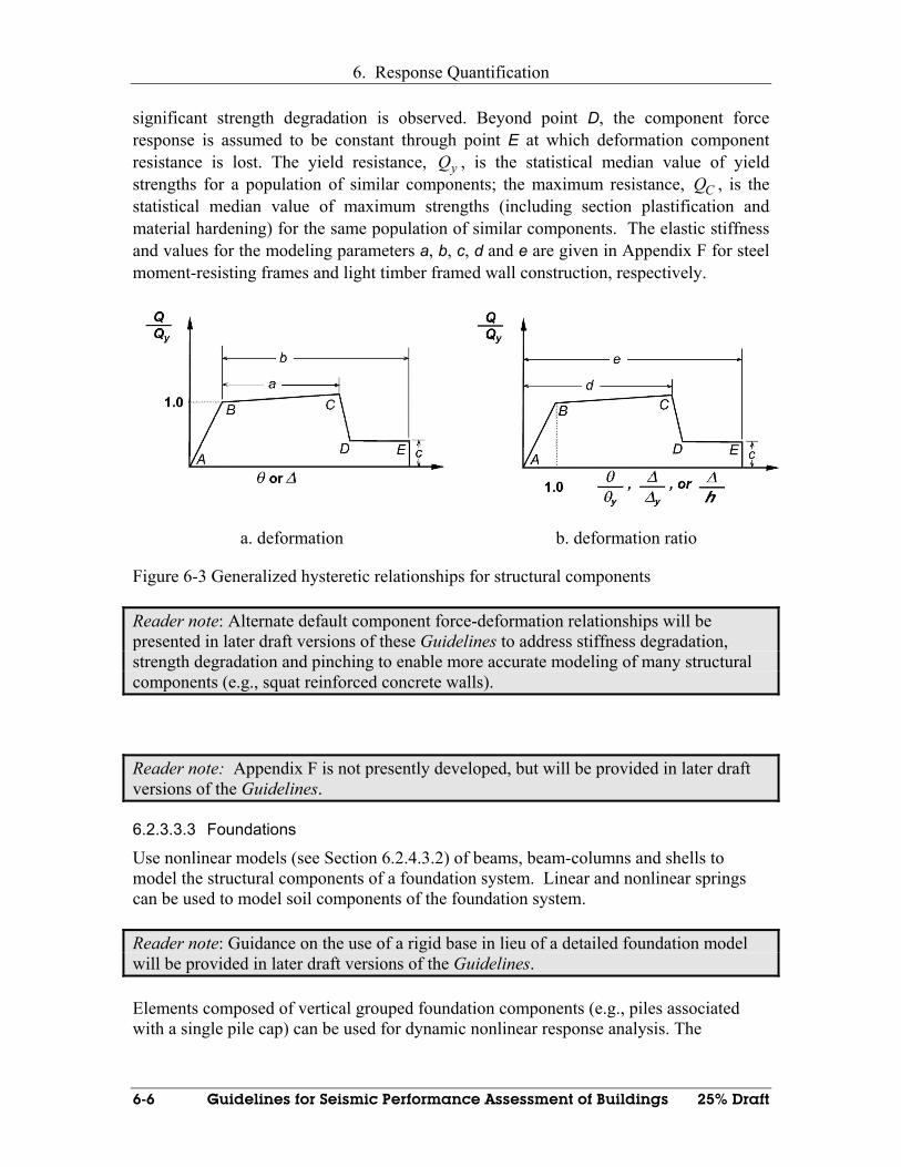
6. Response Quantification
6-6 Guidelines for Seismic Performance Assessment of Buildings 25% Draft
significant strength degradation is observed. Beyond point D, the component force response is assumed to be constant through point E at which deformation component resistance is lost. The yield resistance, yQ , is the statistical median value of yield strengths for a population of similar components; the maximum resistance, CQ , is the statistical median value of maximum strengths (including section plastification and material hardening) for the same population of similar components. The elastic stiffness and values for the modeling parameters a, b, c, d and e are given in Appendix F for steel moment-resisting frames and light timber framed wall construction, respectively.
a. deformation b. deformation ratio
Figure 6-3 Generalized hysteretic relationships for structural components
Reader note: Alternate default component force-deformation relationships will be presented in later draft versions of these Guidelines to address stiffness degradation, strength degradation and pinching to enable more accurate modeling of many structural components (e.g., squat reinforced concrete walls).
Reader note: Appendix F is not presently developed, but will be provided in later draft versions of the Guidelines.
6.2.3.3.3 Foundations
Use nonlinear models (see Section 6.2.4.3.2) of beams, beam-columns and shells to model the structural components of a foundation system. Linear and nonlinear springs can be used to model soil components of the foundation system.
Reader note: Guidance on the use of a rigid base in lieu of a detailed foundation model will be provided in later draft versions of the Guidelines.
Elements composed of vertical grouped foundation components (e.g., piles associated with a single pile cap) can be used for dynamic nonlinear response analysis. The

6. Response Quantification
25% Draft Guidelines for Seismic Performance Assessment of Buildings 6-7
hysteretic properties of each element under generalized loadings should be developed using principles of engineering mechanics.
6.2.3.3.4 Diaphragms
Model diaphragms with realistic assumptions as to their stiffness and strength. A diaphragm can be classified as rigid if the maximum lateral deformation of the diaphragm is less than one half of the average story drift in the vertical components and elements above and below the subject diaphragm. In buildings containing out-of-plane offsets in vertical lateral-force-resisting elements, diaphragms at transition in plan location of the vertical elements should not be considered rigid.
Model diaphragms that are not rigid using shell or membrane finite elements. Diaphragms supporting nonstructural components that are sensitive to vertical acceleration should be modeled as flexible components using shell elements.
Model the distribution of mass across the footprint of a floor diaphragm so as to capture the vertical dynamic response of the diaphragm and the supported nonstructural components, and the torsional response of the diaphragm (see Section 6.2.3.3.5).
6.2.3.3.5 Torsion
Use three-dimensional numerical models of buildings for performance assessment and loss computations if the maximum horizontal displacement at any point on a floor diaphragm exceeds 110% of the average horizontal displacement of the floor diaphragm. Accidental torsion need not be considered for the purpose of performance assessment and loss computations.
6.2.3.3.6 Hysteretic models of nonstructural components
Explicitly model nonstructural components that contribute significant lateral strength and/or lateral stiffness to the building, as characterized in Section 6.2.3.2. Nonlinear models using either beam-column, membrane or shell finite elements are used for such nonstructural components (including the connection hardware). Numerical models of nonstructural components should be based on full-scale cyclic test data. Default numerical models for selected nonstructural components are provided in Appendix F.
6.3 Methods of Analysis
6.3.1 Introduction For conceptual level assessment use either linear static analysis, in accordance with Section 6.3.2, or nonlinear dynamic analysis in accordance with Section 6.3.3. For detailed level assessments, use nonlinear dynamic analysis in accordance with Section 6.3.3.

6. Response Quantification
6-8 Guidelines for Seismic Performance Assessment of Buildings 25% Draft
6.3.2 Linear static response analysis
6.3.2.1 Introduction
Perform linear static analysis as described in detail in Section 3.3.1 of FEMA 356 (FEMA, 2000); as modified in Section 6.3.2.2 below. Lumped parameter models of the framing system can be used for linear static analysis. Median deformation demands are computed using equations (6-1) through (6-4); compute dispersion in the deformation demand using equation (6-5) and the data of Table 6.1.
6.3.2.2 Earthquake excitation
Earthquake shaking is defined by a 5-percent damped acceleration response spectrum, derived in accordance with Chapter 5.
6.3.2.3 Response analysis
To compute median story drift demands, calculate the pseudo lateral load, V, using the formula:
1 2 1 1( , )aV C C S T Wξ= (6-1)
where 1C is an adjustment factor for inelastic displacements; 2C is an adjustment factor for cyclic degradation; 1 1( , )aS T ξ is the spectral acceleration at the fundamental period and damping ratio of the building, in the direction under consideration, for the selected level of ground shaking; and W is the weight of the building. The adjustment factor 1C is computed as:
1 1
121
1
11 for 0.2sec0.04
11 for 0.2 1.0sec
=1 for 1.0sec
RC Ta
R TaT
T
−= + ≤
−= + < ≤
>
(6-2)
where 1T is the fundamental period of the building in the direction under consideration, a is a function of the soil site class per Section 5.3 (= 130, 130, 90, 60 and 60 for site classes A, B, C, D and E, respectively) and R is a strength ratio given by
1 1
1
( , )a
y
S T WRVξ
= (6-3)
where 1yV is the estimated story yield strength at the effective base of the building, and
all other terms have been defined above. The adjustment factor 2C is computed as:
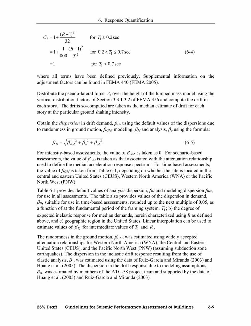
6. Response Quantification
25% Draft Guidelines for Seismic Performance Assessment of Buildings 6-9
2
2 1
2
121
1
( 1)1 for 0.2sec32
1 ( 1)1 for 0.2 0.7sec800
=1 for 0.7sec
RC T
R TT
T
−= + ≤
−= + < ≤
>
(6-4)
where all terms have been defined previously. Supplemental information on the adjustment factors can be found in FEMA 440 (FEMA 2005).
Distribute the pseudo-lateral force, V, over the height of the lumped mass model using the vertical distribution factors of Section 3.3.1.3.2 of FEMA 356 and compute the drift in each story. The drifts so-computed are taken as the median estimate of drift for each story at the particular ground shaking intensity.
Obtain the dispersion in drift demand, βD, using the default values of the dispersions due to randomness in ground motion, βGM, modeling, βM and analysis, βa using the formula:
222MaGMD ββββ ++= (6-5)
For intensity-based assessments, the value of βGM is taken as 0. For scenario-based assessments, the value of βGM is taken as that associated with the attenuation relationship used to define the median acceleration response spectrum. For time-based assessments, the value of βGM is taken from Table 6-1, depending on whether the site is located in the central and eastern United States (CEUS), Western North America (WNA) or the Pacific North West (PNW).
Table 6-1 provides default values of analysis dispersion, βa and modeling dispersion βm, for use in all assessments. The table also provides values of the dispersion in demand, βD, suitable for use in time-based assessments, rounded up to the next multiple of 0.05, as a function of a) the fundamental period of the framing system, 1T ; b) the degree of expected inelastic response for median demands, herein characterized using R as defined above, and c) geographic region in the United States. Linear interpolation can be used to estimate values of Dβ for intermediate values of 1T and R .
The randomness in the ground motion, βGM, was estimated using widely accepted attenuation relationships for Western North America (WNA), the Central and Eastern United States (CEUS), and the Pacific North West (PNW) (assuming subduction zone earthquakes). The dispersion in the inelastic drift response resulting from the use of elastic analysis, βa, was estimated using the data of Ruiz-Garcia and Miranda (2003) and Huang et al. (2005). The dispersion in the drift response due to modeling assumptions, βm, was estimated by members of the ATC-58 project team and supported by the data of Huang et al. (2005) and Ruiz-Garcia and Miranda (2003).

6. Response Quantification
6-10 Guidelines for Seismic Performance Assessment of Buildings 25% Draft
Table 6-1 Default values of dispersion for linear static response analysis
βGM1 Dβ
1T (sec)
e
y
VRV
= βa βm WNA CEUS PNW WNA CEUS PNW
≤ 1.00 0 0.10 0.60 0.55 0.80 2 0.55 0.10 0.80 0.80 1.00 4 0.90 0.15 1.10 0.95 1.25 6 0.90 0.20 1.10 1.10 1.25
0.20
≥ 8 0.90 0.20
0.57 0.53 0.80
1.10 1.10 1.25 ≤ 1.00 0 0.10 0.65 0.60 0.85
2 0.30 0.10 0.70 0.65 0.90 4 0.60 0.15 0.90 0.85 1.05 6 0.70 0.20 0.95 0.95 1.10
0.35
≥ 8 0.75 0.20
0.60 0.55 0.80
1.00 1.00 1.15 ≤ 1.00 0 0.10 0.65 0.60 0.85
2 0.30 0.10 0.70 0.65 0.90 4 0.55 0.15 0.85 0.80 1.00 6 0.65 0.20 0.95 0.90 1.05
0.5
≥ 8 0.70 0.20
0.60 0.55 0.80
0.95 0.95 1.10 ≤ 1.00 0 0.10 0.65 0.60 0.85
2 0.30 0.10 0.75 0.70 0.90 4 0.55 0.15 0.85 0.85 1.00 6 0.65 0.20 0.95 0.90 1.05
0.75
≥ 8 0.70 0.20
0.63 0.58 0.80
1.00 0.95 1.10 ≤ 1.00 0 0.10 0.70 0.65 0.85
2 0.30 0.10 0.75 0.70 0.90 4 0.55 0.15 0.90 0.85 1.00 6 0.60 0.20 0.95 0.95 1.05
1.0
≥ 8 0.65 0.20
0.65 0.60 0.80
0.95 0.95 1.05 ≤ 1.00 0 0.10 0.70 0.65 0.90
2 0.25 0.10 0.75 0.70 0.90 4 0.40 0.15 0.85 0.75 1.00 6 0.50 0.20 0.90 0.85 1.05
1.50
≥ 8 0.55 0.20
0.68 0.60 0.85
0.90 0.85 1.05 ≤ 1.00 0 0.10 0.75 0.65 0.95
2 0.25 0.10 0.75 0.70 0.95 4 0.35 0.15 0.80 0.75 1.00 6 0.45 0.20 0.90 0.80 1.05
2.0+
≥ 8 0.50 0.20
0.70 0.60 0.90
0.90 0.85 1.05 1. WNA = Western North America; CEUS = Central and Eastern United States; PNW = Pacific
Northwest. Values established using the attenuation relationships of Abrahamson and Silva (1997) for WNA, Campbell (2003) for CEUS, and Atkinson and Boore (2003) for the PNW; and moment magnitudes between 6.5 and 7.0.
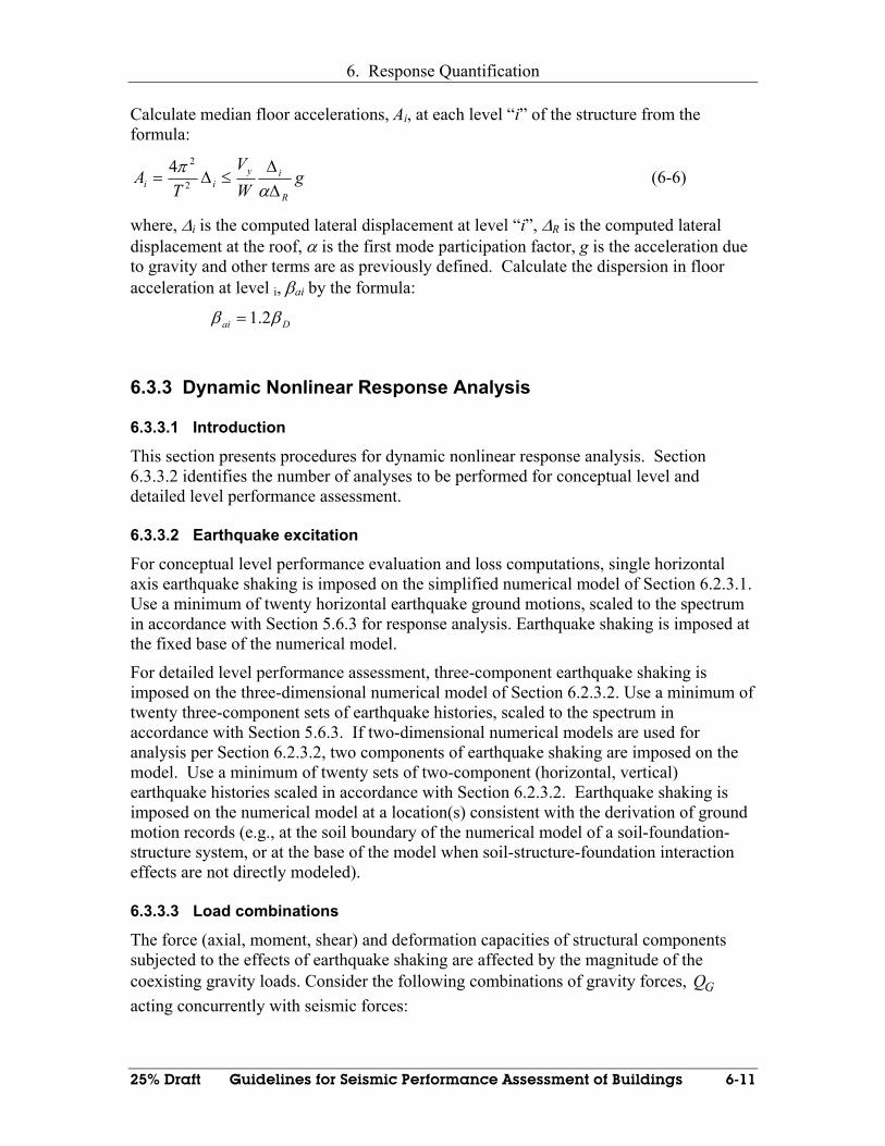
6. Response Quantification
25% Draft Guidelines for Seismic Performance Assessment of Buildings 6-11
Calculate median floor accelerations, Ai, at each level “i” of the structure from the formula:
gWV
TA
R
iyii ∆
∆≤∆=
απ
2
24 (6-6)
where, ∆i is the computed lateral displacement at level “i”, ∆R is the computed lateral displacement at the roof, α is the first mode participation factor, g is the acceleration due to gravity and other terms are as previously defined. Calculate the dispersion in floor acceleration at level i, βai by the formula:
Dai ββ 2.1=
6.3.3 Dynamic Nonlinear Response Analysis
6.3.3.1 Introduction
This section presents procedures for dynamic nonlinear response analysis. Section 6.3.3.2 identifies the number of analyses to be performed for conceptual level and detailed level performance assessment.
6.3.3.2 Earthquake excitation
For conceptual level performance evaluation and loss computations, single horizontal axis earthquake shaking is imposed on the simplified numerical model of Section 6.2.3.1. Use a minimum of twenty horizontal earthquake ground motions, scaled to the spectrum in accordance with Section 5.6.3 for response analysis. Earthquake shaking is imposed at the fixed base of the numerical model.
For detailed level performance assessment, three-component earthquake shaking is imposed on the three-dimensional numerical model of Section 6.2.3.2. Use a minimum of twenty three-component sets of earthquake histories, scaled to the spectrum in accordance with Section 5.6.3. If two-dimensional numerical models are used for analysis per Section 6.2.3.2, two components of earthquake shaking are imposed on the model. Use a minimum of twenty sets of two-component (horizontal, vertical) earthquake histories scaled in accordance with Section 6.2.3.2. Earthquake shaking is imposed on the numerical model at a location(s) consistent with the derivation of ground motion records (e.g., at the soil boundary of the numerical model of a soil-foundation-structure system, or at the base of the model when soil-structure-foundation interaction effects are not directly modeled).
6.3.3.3 Load combinations
The force (axial, moment, shear) and deformation capacities of structural components subjected to the effects of earthquake shaking are affected by the magnitude of the coexisting gravity loads. Consider the following combinations of gravity forces, GQ acting concurrently with seismic forces:

6. Response Quantification
6-12 Guidelines for Seismic Performance Assessment of Buildings 25% Draft
LDG QQQ 0.11.1 += (6-6)
where DQ is the dead-load effect, and QL the best estimate of the permanent live load (with a default value of 25% of the unreduced design live load).
6.3.3.4 Verification of analysis assumptions
The numerical models of structural and nonstructural components of Section 6.2 and Appendix F will generally be based on a series of assumptions, including loading history (cyclic, monotonic, repeated), loading rate, bi- or tri-directional loading and deformation effects, peak deformation and rate of stiffness and/or strength degradation. These assumptions should be verified for each structural and nonstructural component following nonlinear response-history analysis and before values of demand parameters are mined and statistically sorted and interpreted for fragility calculations per Section 6.4 and Chapter 7.
6.3.3.5 Median and Dispersion Values
The various demand parameters used to predict building damage are not independent. A ground motion record that produces relatively large interstory drifts will likely produce large forces and displacements throughout the structure. Similarly, a ground motion that produces moderate interstory drifts will likely also produce moderate floor accelerations throughout the structure. To account for the relationships between the various demands used to predict damage in a building, it is necessary to construct joint probability distributions of the demand parameters from the data set of statistics obtained from the analyses, that account for these inter-relationships between the demand parameters obtained from individual analyses.
To form such joint probability distributions it is necessary to pick a single demand parameter, for example peak roof displacement, in a given direction of response that all other demands in the direction of response can be indexed to. The following procedure can be followed.
1. Examine the data from the analyses and for each ground motion analyzed, pick out the peak value of an index demand parameter, Di. Roof drift will often be a convenient index parameter. Since building response is often uncoupled in two primary orthogonal directions, a separate index parameter should be selected in each direction, e.g. peak roof displacement in the north-south direction and peak roof displacement in the east-west direction.
2. Using the procedures of Appendix A, determine the median value iD and dispersion, βDi for each index demand, Di. Note that since ground motion is bi-directional, sometimes a peak quantity obtained from an analysis will be positive and other times negative. From a perspective of predicting damage, it does not matter whether the peak demand is positive or negative, and in fact it must be considered that regardless of the sign predicted by the analysis, any peak could demand could be either positive or negative. Therefore, for the purposes of

6. Response Quantification
25% Draft Guidelines for Seismic Performance Assessment of Buildings 6-13
determining peak demands and medians and dispersions of these demands, the absolute values of the peak quantities obtained from the analyses should be used.
3. For each ground motion and each demand parameter that will be used to predict damage, Dj , determine the ratio of the absolute value of the peak parameter value, Dj; to Di, called here, Rji, for each direction of building response.
4. For each demand parameter, Dj, determine the dispersion value of the ratios, Rji, designated herein as jiRβ
Each of the demand dispersions, obtained from the suite of analyses, using the above procedures must be modified to account for inherent uncertainty in the ground motion intensity using the formula:
2 2i iD D GMβ β β′ = + (6-7)
2 2R R GMji jiβ β β′ = + (6-8)
where, βGM is the dispersion due to ground motion, taken as 0 for intensity-based assessments, taken as the value associated with the attenuation relationship used to obtain the spectrum for scenario-based assessments, and obtained from Table 6-1 for time-based assessments;
iDβ ′ is the dispersion in the index demand and R jiβ ′ is the dispersion in the ratios considering the ground motion variability.
For conceptual level assessments, the demand parameters of interest are the peak interstory drift at each level of the structure and the peak floor acceleration at each level of the structure, in each of two horizontal directions of shaking. For detailed level assessments, in addition to the demand parameters of interest for conceptual level assessments, additional parameters may be of interest.
With the values of the median and dispersion of the index parameter and the dispersion of the ratio of each demand parameter of interest to the index parameter it is possible to predict a large number of sets of earthquake responses for the structure that are statistically and structurally consistent, without having to conduct large numbers of nonlinear dynamic analyses. The procedure for doing this is described in Chapters 3, 7 and 8.
6.4 Demands on Nonstructural Components and Systems and Contents
6.4.1 Demands from Analysis of Structures For a given ground motion intensity level, analyze the structure as described in Section 6.3.2 o4 6.3.3. The analysis will predict demands at each floor level and at the roof, which provide meaningful demands on nonstructural components. For conceptual level assessments, response will be obtained from the structural analysis in each of two primary orthogonal directions of response, at the center of mass of each diaphragm level. For detailed assessments, demands will be developed in each horizontal direction at the center and edges of the building and vertically at the center and edges of floors. As a

6. Response Quantification
6-14 Guidelines for Seismic Performance Assessment of Buildings 25% Draft
minimum, determine median and dispersion values for the following demands parameters:
1. Peak floor acceleration
2. Peak spectral floor acceleration at periods of 0.2 seconds, 0.5 seconds and 1 second.
3. Peak inter-story drift.
These demands are used directly to assess performance of nonstructural components using the fragility functions discussed in Chapter 8 and the default fragility function characteristics provided in Appendix E.
6.4.2 Equivalent Static Analysis
6.4.2.1 Analysis detail
For many nonstructural components, seismic performance is directly related to a significant degree to the adequacy of anchorage and bracing. For conceptual level assessments, evaluation of anchorage and supports will not be required and fragility of components and systems will be based on default values. However for detailed assessment, evaluate the capacity of typical anchorage and bracing of nonstructural high consequence nonstructural components using simplified linear static analysis, with forces calculated using the accelerations obtained from the structural analysis. Typically, an equivalent static analysis would be performed of items that are only floor or ceiling supported. In some very special cases a dynamic analysis may be performed of a nonstructural system such as a critical piping system. Such instances are expected to be very rare.
6.4.2.2 Anchorage and bracing analysis
Evaluate anchorage and bracing first by treating the item being assessed as a single degree of freedom system. Compute the fundamental component period of the item, Tp, as:
⎟⎟⎠
⎞⎜⎜⎝
⎛=
gKW
Tp
pp 159.0 (6-8)
Where Wp = seismic weight of the component
Kp = fixed base period of component including bracing and anchorage
g = acceleration of gravity
Determine the floor spectra for the floor or ceiling where the item is attached from the structural analysis. Determine the spectral response acceleration for the component, Sap from the floor spectra, at the period T. Using the spectral value and seismic weight the component static seismic force demand is determined as:
appp SWF = (6-9)
6. Response Quantification
25% Draft Guidelines for Seismic Performance Assessment of Buildings 6-15
Apply the component static seismic force calculated from equation 6-9 at the center of mass of the item being evaluated and compute the anchorage and bracing forces.
It should be noted that by comparing the static analysis demand with the capacities of bracing and anchorage one can estimate when the demand equals the capacity. From an understanding of this point, one can establish one point of the fragility function namely the high confidence low probability of failure point. This is the point where the component and its bracing and anchorage are still elastic and where the probability of failure is considered remote. Procedures for translating the high confidence low probability point to a full fragility function are provided in Appendix E.
6.4.2.3 Load path analysis to primary structural system
In addition to evaluating anchorage and bracing, for some components it is necessary to verify the adequacy of the load path for anchorage and bracing forces from the point of attachment to the primary structural system. This is especially important for roof mounted equipment in existing buildings where the item of equipment may be supported on a concrete pad which may not be tied to the primary structural system. Premature failure of a load path may result in a significant reduction of component fragility. To evaluate the load path, take the component static seismic force as determined in Section 6.3.2.2 and evaluate the adequacy of the load path following the anchorage and bracing forces far enough into the structure to where they are unlikely to directly result in a damage mode. Like the anchorage and bracing, the resulting load path forces should be compared with member and connection capacities. if the demand is greater than the capacity at a lower point than the component itself, then the lowest capacity point may govern the high confidence low probability of failure point determination.
6.4.3 Dynamic Analysis of Distributed Systems
6.4.3.1 Analysis detail
For detailed level assessments, it may be necessary to perform three-dimensional dynamic analyses of spatially distributed nonstructural systems such as piping and ductwork. This is justified if it is determined that the losses associated from such systems are a major contributor to the overall losses associated with the building. For such analyses, prepare sub-structural models of the nonstructural system in a manner analogous to that of the building structure and incorporate this substructure model into the building structural model at the points of attachment between the nonstructural system and the building. Typically an elastic substructure model will be sufficient to establish the demand on connections and anchorage. However, in some extremely rare instances, a nonlinear analysis of such systems may be required. In such cases the nonlinear demands on the most vulnerable links in the system such as threaded connections is determined. For such cases the fragility functions of the connections are typically determined by tests and thus the demands can be compared directly with the fragility functions in order to determine the damage state for a particular realization.
The installation of many nonstructural systems, particularly seismic bracing for ceiling systems and HVAC ducting may not be particularly well controlled. This lack of installation control results because these components are not considered as part of the

6. Response Quantification
6-16 Guidelines for Seismic Performance Assessment of Buildings 25% Draft
seismic design. Therefore, at times, installation of these systems must be considered questionable. In such cases, a larger variability or lower median fragility should be assumed to account for this lack of confidence regarding the installation. If an existing installation is being assessed, a thorough walkdown of the system can permit a more direct assessment of the installation, which can permit, can improve confidence regarding the installed seismic capacity.
6.4.3.2 Other concurrent loads and load combinations
In determining the demands on nonstructural components, other loads, which are typically present during the operation of the components, should be included in the analysis. For example dead loads of the component, fluid loads and pressure loads should be included if they would effect the demand on the component’s seismic force resisting system. Thermal loads may also be included but it should be noted that thermal loads are self straining loadings and should therefore be treated as strain demands rather that force demands. Care should be taken when combining thermal loading with seismic loads. Earthquake loads are not typically combined with other short term natural hazards such as wind.

25% Draft Guidelines for Seismic Performance Assessment of Buildings 7-1
7 Structural Damage Assessment
7.1 Introduction This chapter presents the general methodology to identify relevant damage states for structural systems and to develop, either experimentally or numerically, fragility functions for these damage states. Section 7.2 introduces damage states for structural components, elements and systems for direct loss, indirect loss and casualty computations. General procedures to develop structural fragilities are presented in Section 7.3. Default fragility functions are presented in the appendices for selected components of subtypes of framing systems1.
7.2 Structural Damage States
7.2.1 General Structural damage states serve as the link between numerical simulation (response-history analysis) and loss computations. Since loss computation is the key outcome of the performance assessment, damage states are defined herein in terms of either the degree or scope of repair (for direct and indirect losses) or percentage of building collapse (for casualty computations). Both definitions are intended to facilitate a straightforward computation of loss.
Damage is a continuum and not a series of discrete states. (One example is the amplitude of steel beam flange local buckling for which amplitude is a continuous function of beam deformation.) However, direct loss is not a continuous function (of beam deformation in this example) because modest increases in the level of damage can trigger large increments in construction activity and cost (e.g., shoring of multiple levels of building framing).
Multiple damage states (e.g., DS1, DS2, DS3) are typically identified for each structural component and presented in the form of a family of fragility curves. Damage states are ordered in terms of increasing damage (i.e., the damage in state DS2 exceeds that of DS1) for fragility and loss computations. Fragility relations described in Section 7.3 are used to present the distributions of each damage state as a function of a critical demand parameter.
Building-specific damages states should be developed for those framing systems for which default fragility curves are unavailable. The process used to develop default fragility curves is contained in Appendix C.
1 Herein, framing systems are high-level descriptions of material type, means of force transfer, and construction detailing (e.g., special steel moment-resisting frame). Subtypes of framing systems are lower level descriptions (e.g., pre-1994 steel moment frame; welded flange, bolted web connection).

7. Structural Damage Assessment
7-2 Guidelines for Seismic Performance Assessment of Buildings 25% Draft
7.2.2 Direct Economic Loss
7.2.2.1 Introduction
Damage states for direct economic loss computations are defined for the default fragility curves of Appendices D and E in terms of structural damage and discrete states of component (e.g., beam, column, connection, wall) repair. Direct losses are then computed on a component-by-component basis, conditional on value(s) of component demand and aggregated using the procedures of Section 9.
Default damage states for direct economic loss are presented in Appendices D and E for steel moment-frame and light frame wood shear wall construction, respectively. The procedures used to establish the damage states are presented in the relevant appendix. Alternate damage states for these framing systems are permissible.
Damage states for framing systems and their components shall be developed and documented using the following guiding principles.
1. Components of a structural framing system that are likely to be damaged in earthquake shaking, or have been damaged in past earthquakes, shall be identified.
2. The types of damage recorded in past earthquakes or following experimentation shall be documented for each component of item 1,
3. Damage states and fragility curves shall be developed for all components of item 1.
4. A minimum of two damage states shall be established for each structural component of item 1.
5. Damage states (DS1, DS2….DSn) for each structural component shall be presented in order of increasing damage and cost of repair.
6. Detailed descriptions of each damage state shall be documented.
7. Damage states and the associated demand parameter(s) must be predictable by structural analysis codes.
8. Detailed descriptions of repair or replacement should be provided for each damage state and each structural component.
7.2.3 Downtime Decisions regarding the continued occupancy and functionality of a building1 are made by both regulators and building owners. All decisions are impacted by the regional and
1 The differences between continued occupancy and functionality vary by occupancy type. For some occupancy types (e.g., a semiconductor fabrication plant), occupancy without functionality (which would require utilities and a means to transport staff to and from the building) makes no
7. Structural Damage Assessment
25% Draft Guidelines for Seismic Performance Assessment of Buildings 7-3
local availability of transportation and utilities (e.g., power, water, gas). The default fragility curves of Appendices D and E assume the following:
1. All utilities (including power, water and gas) are available immediately following the earthquake.
2. Decisions regarding occupation of the building are made by the owner and her/his engineering design professionals only.
3. Contracting services and related resources (including engineering design professionals) are available immediately following the earthquake to begin retrofit design and repair work.
4. The probability of interruption (and loss of function) is 0 in the absence of damage.
5. Equipment that is critical to the ongoing function of a building or facility can be easily relocated with no loss of service.
6. There is no indirect loss associated with the replacement of equipment damaged by the failure of structural framing.
7. The interruption times for all floors above and below a story that has collapsed is the same.
In this Guideline, computations of interruption time (or time to full recovery) due to structural damage are based on performance assessments at the story level. Damage states for the default fragility curves of Appendices D and E are defined herein by repair times, with a minimum repair time of one month based on past experience. (Once a building is identified as needing repair, retrofit or repair designs must be developed, building permits must be obtained, a contractor must be retained and the selected contractor must complete the work.) The default interruption times used in this Guideline associated with structural damage are one month, three months, 6 months, 12 months and 2 years. The story-level response quantities of peak and permanent story drift are used as the demand parameters for indirect loss computations.
Appendix D provides the technical basis and rationale for the damage states that are associated with the different interruption times.
7.2.4 Casualties This Guideline assumes two sources of casualties for the purpose of loss computations, namely, 1) partial or total collapse of structural framing, and 2) failure of perimeter nonstructural components such as precast cladding and exterior glazing. Only the first source is addressed in this section and the corresponding appendices.
Collapse of structural framing represents a failure at the system level and is due principally to excessive story drift, where the values assigned to excessive are framing-system dependent. (For example, a modern steel moment-frame system should sustain
economic sense. For other occupancy types (e.g., an apartment block), occupancy without full functionality (e.g., elevators, power) is possible.

7. Structural Damage Assessment
7-4 Guidelines for Seismic Performance Assessment of Buildings 25% Draft
peak story drifts in excess of 5% of the story height whereas a nonductile concrete moment frame building might collapse at drift levels of less than 1% of the story height.) System failures are triggered by the failure of multiple components (e.g., columns, joints, connections) and no single local level demand parameter (e.g., rotation [of a connection], axial force [in a column]) is a reliable demand parameter for system-level failures. Herein, story drift is assumed to be the most robust demand parameter for assessing the likelihood of a partial or total collapse of the building frame.
Default damage states are assumed in this Guideline for casualty computations, namely, 1) partial collapse of a floor system at one level of a building (see Figure 7-1a: the partial collapse of a Kaiser building during the 1994 Northridge earthquake); 2) collapse of a story of a building (see Figure 7-1b: the collapse of one story of the Kobe City Hall during the 1995 Great Hanshin earthquake); and 3) total building collapse (see Figure 7-1d: the total collapse of a building near Golcuk during the 1999 Koacheli earthquake.) Casualties due to building overturning (see Figure 7-1c: overturning of a building in downtown Kobe during the 1995 Great Hanshin earthquake) are not accounted for in this Guideline.
a. part floor collapse b. story collapse
c. building overturning d. building collapse
Figure 7-1 Damage states for casualty calculations
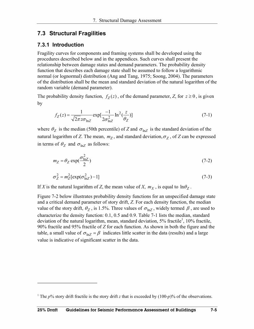
7. Structural Damage Assessment
25% Draft Guidelines for Seismic Performance Assessment of Buildings 7-5
7.3 Structural Fragilities
7.3.1 Introduction Fragility curves for components and framing systems shall be developed using the procedures described below and in the appendices. Such curves shall present the relationship between damage states and demand parameters. The probability density function that describes each damage state shall be assumed to follow a logarithmic normal (or lognormal) distribution (Ang and Tang, 1975; Soong, 2004). The parameters of the distribution shall be the mean and standard deviation of the natural logarithm of the random variable (demand parameter).
The probability density function, ( )Zf z , of the demand parameter, Z, for 0z ≥ , is given by
22
ln ln
1 1( ) exp[ In ( )]2 2Z
ZZ Z
zf zz θπ σ σ
−= (7-1)
where Zθ is the median (50th percentile) of Z and lnZσ is the standard deviation of the natural logarithm of Z. The mean, Zm , and standard deviation, Zσ , of Z can be expressed in terms of Zθ and lnZσ as follows:
2lnexp( )2
ZZ Zm σθ= (7-2)
2 2 2ln[exp( ) 1]Z Z Zmσ σ= − (7-3)
If X is the natural logarithm of Z, the mean value of X, Xm , is equal to ln Zθ .
Figure 7-2 below illustrates probability density functions for an unspecified damage state and a critical demand parameter of story drift, Z. For each density function, the median value of the story drift, Zθ , is 1.5%. Three values of lnZσ , widely termed β , are used to characterize the density function: 0.1, 0.5 and 0.9. Table 7-1 lists the median, standard deviation of the natural logarithm, mean, standard deviation, 5% fractile1, 10% fractile, 90% fractile and 95% fractile of Z for each function. As shown in both the figure and the table, a small value of lnZσ β= indicates little scatter in the data (results) and a large value is indicative of significant scatter in the data.
1 The p% story drift fractile is the story drift z that is exceeded by (100-p)% of the observations.

7. Structural Damage Assessment
7-6 Guidelines for Seismic Performance Assessment of Buildings 25% Draft
0.00
0.05
0.10
0.15
0 2 4 6 8Story drift (% of story height)
f Z(z
)
Beta = 0.1Beta = 0.5Beta = 0.9
Figure 7-2 Density functions for 1.5Zθ = and ln 0.1,0.5,0.9Zσ =
Table 7-1 Parameters and values of the density functions of Figure 7-1 Fractile story drift
Zθ InZσ Zm Zσ 5% 10% 90% 95%
1.50% 0.10 1.51% 0.15% 1.27% 1.32% 1.70% 1.76%
1.50% 0.50 1.70% 0.91% 0.66% 0.79% 2.84% 3.41%
1.50% 0.90 2.25% 2.51% 0.34% 0.47% 4.74% 6.59%
Figure 7-3 presents the three density functions of Figure 7-2 and Table 7-1 as probability (cumulative) distribution functions. Each of these cumulative distribution functions could represent a fragility curve associated with a damage state. The fragility curve could be defined in terms of a) Zθ and lnZσ ); b) Zθ and a fractile (e.g., 95% and the corresponding value of z), and c) two fractiles (e.g., 5% and 95% and the corresponding values of z).
0.0
0.2
0.4
0.6
0.8
1.0
0 2 4 6 8
Story drift (% of story height)
P (D
S >
DSi
)
Beta = 0.1Beta = 0.5Beta = 0.9
Figure 7-2 Fragility curves for 1.5Zθ = and ln 0.1,0.5,0.9Zσ =

7. Structural Damage Assessment
25% Draft Guidelines for Seismic Performance Assessment of Buildings 7-7
7.3.2 General Procedures Fragility curves for components of framing systems, elements of framing systems and framing systems can be computed by multiple methods that rely on experimental data, numerical simulation data, expert judgment or a combination of one or more methods.
Probability density functions, ( )Zf z , must be established for each damage state and each component. These density functions must be integrated from 0 to ∞ to generate the corresponding probability (cumulative) distribution function or fragility curve.
The lack of data will generally prevent the user from defining Zθ and lnZσ on the basis of experimentation alone because more than 200 independent observations are likely needed (Soong 2005). If a large dataset of experimental and validated numerical results is available, the parameters of the distribution can be established using well-established procedures available in widely used software.
If a large dataset is unavailable, experimental and numerical data should be augmented by expert engineering judgment to establish Zθ and lnZσ . One procedure to compute these parameters is to estimate the median value based on a combination of simulation (physical and numerical) and a fractile, say 5% or 10%, with the corresponding value of the random variable (demand parameter). Assuming that the data (observations) follow a lognormal distribution with a median Zθ , the standard deviation of the natural logarithm of the distribution can be calculated as
ln
ln( )i
zZ
zθσλ
= − (7.3-4)
where λ = 1.64 and 1.28 for the 5% and 10% fractiles, respectively, and iz is the corresponding value of the demand parameter. For example, consider a damage state, such as steel beam flange local buckling of amplitude 0.5 inch, that is characterized in part by a median story drift of 1.5% (= Zθ ). If, based on a combination of simulation and judgment, it is expected that such flange local buckling will develop in no more than 5% of specimens at a story drift of 1.05%, the standard deviation of the natural logarithm of the distribution can be calculated as
ln
1.05ln( ) ln( )1.50 0.217
1.64
i
zZ
zθσλ
= − = − = (7-4)
Fragility curves should be established for individual structural components using the critical demand parameter for that component. A curve must be established for each damage state identified for that component. The product of such computations will be a family of fragility curves, such as that shown in Figure 7-4, for three damage states, DS1, DS2 and DS3, where the damage in state DS2 exceeds that in state DS1, and that in state DS3 exceeds that in state DS2. Connection rotation is used as the critical demand

7. Structural Damage Assessment
7-8 Guidelines for Seismic Performance Assessment of Buildings 25% Draft
parameter for the component of Figure 7-4. In this figure, 1.5, 2.5,3.5Zθ = % and
ln 0.3,0.4,0.5Zσ = for DS1, DS2 and DS3, respectively.
0.0
0.2
0.4
0.6
0.8
1.0
0 2 4 6 8
Connection rotation (% radian)
P (D
S >
DSi
)
DS1DS2DS3
Figure 7-4 Family of fragility curves for a hypothetical structural component
7.3.3 Default Fragility Functions Default fragility functions are presented in Appendices D and E for steel moment-resisting frames and light frame wood shear wall buildings, respectively. Three loss states are addressed with the default fragility functions, namely,
• Direct losses
• Downtime
• Casualties
Fragility curves are provided for schematic-level and detailed level performance assessment and loss computations. For the schematic-level performance assessment and loss computations, story drift is used as the demand parameter. More refined demand parameters (e.g., plastic hinge rotation) are provided for detailed analysis. Fragility curves are defined for multiple structural damage states as described in Section 7.2.1. Descriptions of each damage state are provided for every fragility curves.
The default families of fragility functions presented in the appendices were developed for selected components of subtypes of framing systems. Limitations on the range of applicability of these fragility curves are identified in the appendices. Most of these limitations reflect the scope of the dataset upon which the fragility curves are based. The procedures used to develop the default curves are presented to facilitate improvements at a later date if additional information becomes available.

25% Draft Guidelines for Seismic Performance Assessment of Buildings 8-1
8 Nonstructural Damage Assessment
8.1 Introduction
When nonstructural components and systems located in buildings are subjected to increasing demands imposed by earthquake motions they will eventually be damaged. This damage may be the direct result of shaking induced acceleration or relative displacement exceeding the capacity of the component, or the indirect result of impact with other components or the collapse of other components or the building itself upon the components. When damage occurs, this may result in a variety of consequences, including: a need for some type of repair action, the creation of a hazardous condition, such as toppling of a heavy component or release of flammable material; or creation of an inability to occupy or use a facility, such as might occur if lighting is unavailable or fire protection systems are compromised. The approach used in these Guidelines is to: identify the significant types of damage that can occur in nonstructural components; associate fragility functions with each damage state that predict the likelihood of incurring damage as a function of a demand parameter; and evaluating the consequences of the predicted damage, using consequence functions. The significant types of damage are termed damage states. This section describes the general methodology used to identify relevant damage states for nonstructural systems and components, and to develop or obtain appropriate fragility functions for these damage states. Appendix C provides general information on damage states and fragility functions. Appendix E provides default damage states and fragility functions for typical nonstructural components and systems in selected building occupancies.
8.2 Nonstructural Damage States
8.2.1 General
Damage states are particular to the individual nonstructural component or system. For example, for interior walls, a damage state may be cracks up to 1/8 inch wide. Cracks up to this width can be repaired by simply taping and painting the gypsum board if the wall is constructed of drywall. A second damage state may be cracks are greater than 1/8 inch and less than ½ inch in which case the wall drywall panel may need replacing but the metal studs can remain in place. A third damage state may be where cracks are greater than ½ inch and the wall is in such a condition that the entire wall including studs and sheathing should be replaced. Another example might be piping systems where one damage state might be minor leaks while a second damage state might be a ruptured connection. In Appendix E, damage states that have been identified for the nonstructural architectural and MEP components of significance have been identified as well as damage state for significant contents. In addition, Appendix E, combines these damage states for the default performance groups.
8. Nonstructural Damage Assessment
8-2 Guidelines for Seismic Performance Assessment of Buildings 25% Draft
8.2.2 Casualties
Damage states that result in hazardous conditions or loss of life sustaining function that can result directly in injuries or deaths are deemed to be casualty damage states. In this case, the damage should be directly relatable to possible deaths and injuries depending on the number of people present in the vicinity of the condition or function. For example if a damage state is loss of 10% of the tile on a roof, this could be related to a quantity of roof tiles falling on areas adjacent to a building, which in turn can be related to a number of casualties based on the number of people who are exposed to the hazard. Another example of a system casualty damage state is the loss of emergency power in a hospital. If the power is lost, those folks who are on heart lung machines will likely die. The interruption time for these damage states is therefore directly relatable to probable deaths or injuries. The relationship between damage state and casualties for the nonstructural items of significance and default performance groups is provided in Appendix E.
8.2.3 Direct Economic Loss
Damage states that result in a need for some type of repair or replacement action are deemed to be Significant for direct economic loss. These types of damage states are to be directly relatable to some quantity of repair. For example, a drywall wall area 4 feet wide by 8 feet high will require 10 linear feet of tapping and an area of 32 square feet of painting if the maximum crack widths are 1/8 inch. The relationship between damage state and cost of repair action associated with the items of significance and the default performance groups is provided in Appendix E.
8.2.4 Downtime
Damage states that result in loss of occupancy or cause function interruption are deemed to be downtime damage states. In this case, each damage state must to be directly relatable to some period of time of lost occupancy or use. For example, if a fire sprinkler pipe ruptures on an upper floor, it not only results in repair actions it may also result in red tagging of a building and a loss of occupancy. If the ruptured pipe is a 1 inch line with a pressure of 60 psi and it is assumed that the water will not be turned off for 1 hour from when the line breaks, this can be translated into a volume of water that has leaked onto the floor and then into a period of time that will be associated with clean up and repair. Other possible components where system ruptures could result in loss of occupancy include sewer system leakages and gas line leaks. The relationship between damage state and occupancy/function times associated with the nonstructural items of significance and default performance groups is provided in Appendix E. The downtime consequences of a damage state can be very occupancy-specific.

8. Nonstructural Damage Assessment
25% Draft Guidelines for Seismic Performance Assessment of Buildings 8-3
8.3 Nonstructural Fragilities
As noted previously, fragility functions are the probabilistic relationship between damage state between and demand. These functions can be established by laboratory testing, observation, experience and judgment from actual earthquakes or by analysis. As described in Appendix C, these functions are usually plotted as lognormal function of a probability of incurring a given damage state as a function demand. Fragility functions are specific to individual nonstructural components. Currently the demand parameters most frequently used in established fragility functions for nonstructural components are inter-story drift, peak floor acceleration and peak spectral floor acceleration at the predominant period of the component. . For purpose of these Guidelines, for a given damage state, fragility functions are defined in terms of two parameters: the median value of the demand which the damage state is expected to initiate and the dispersion, which is a measure of the variability or uncertainty associated with predicting damage as a function of demand. Appendices E and F provide additional information on lognormal distributions, their defining parameters, and fragilities.
8.3.1 General Procedures for Establishing Fragility Functions
Procedures for developing fragility functions are provided in Appendix C. In some cases, such as for piping systems, subcomponent fragilities such as for connections may actually be determined by test and then system performances assessed by analysis combined with component testing analogous to how structural performance is assessed on the basis of testing and analysis.
8.3.2 Default Fragility Functions
Default fragility functions that have been established for the nonstructural components of significance and the default performance groups are provided in Appendix E. These functions have been established based on available data as well as expert judgment. Adjustment factors have also been provided that modify the default fragility functions for the factors described earlier in Section 4.5.1. The adjustment factors are also provided in Appendix E.


25% Draft Guidelines for Seismic Performance Assessment of Buildings 9-1
9 Consequence Functions
9.1 Introduction Information on earthquake damage to a building’s components for a particular ground motion realization is obtained in the form of damage states that describe the type and extent of damage within each of the several performance groups. This information must be translated into a measure of losses (i.e. casualties, direct economic loss, downtime). The transition from damage to loss is made using consequence functions. These functions are applied to the total damage state for a building. They are developed for each type of loss and can differ among types of buildings. They are, by nature, complex and uncertain. Often they can be simplified, however, using heuristic procedures and approximations.
The following sections discuss some of the characteristics of consequence functions qualitatively for an example case of damage to several columns within a multistory building. Appendices G and H provide default consequence functions, respectively, for selected structural framing systems and building occupancies.
Reader note: At the time of this 25% draft, consequence functions have been developed only to a conceptual level, and Appendices G and H have not yet been developed. A very simple example for capital losses is illustrated in Chapter 3. It is anticipated that more complete procedures for forming consequence functions, and the content of Appendices G and H, will be provided in later drafts of these Guidelines.
9.2 Casualty functions Casualty losses in a building due to earthquakes are measured in deaths and serious injuries. Casualties can be caused by several conditions:
• Local collapse, where a portion of a building becomes unstable for vertical load and load transfer mechanisms are not sufficient to prevent a portion of the structure from collapsing.
• General collapse of a structure can be caused by a loss of vertical load carrying capability at an entire story, or stories. General collapse can also occur progressively from an initial local vertical load collapse. Excessive horizontal displacements from seismic shaking can result in a sidesway collapse mechanism.
• Falling objects
• Release of hazardous materials
With respect to the example damage to several columns within a building there are several important consideration for the casualty consequence function.
• Were the columns in the same floor level?
• Is there adequate structural capability to transfer vertical loads to other columns?

9. Consequence Functions
9-2 Guidelines for Seismic Performance Assessment of Buildings 25% Draft
• Are the columns part of the seismic force resisting system?
• Is there a potential for the development of a sidesway mechanism?
• What are the uncertainties involved with each potential collapse state?
• How many individuals are exposed to each potential collapse state?
9.3 Direct Economic Loss Functions Capital losses, measured in dollars, are relatively straight forward to determine as a function of a building damage state. The building total damage state (see Chapter 3) comprises a detailed description of the condition of a building after one possible earthquake ground shaking realization. This description is expressed in terms of repair measures that could be given to a contractor for use in developing an estimate of the costs to repair the building and replace its damaged contents. The contractor asked to perform such an estimate would apply unit costs, in terms of labor and materials, to each of the repair actions required to restore the building. When he/she does this, the unit costs are somewhat dependent on the total quantities of basic repair measures required. In some instances (e.g. scaffolding, protection of finishes, clean-up), if damage is widespread, the costs will be distributed to more than a single repair measure. Contractors’ overhead and profit depend on the total amount of work and the type of tradesmen required. The type of repair work performed, and the methods used, will in part depend on how much repair work of a given type is required.
With respect to the example damage to several columns within a building these considerations have several implications for the capital loss consequence function.
• Are the columns located in a single floor?
• What is the total quantity of repair measures for the entire building that apply to the damaged columns?
• Could some of the repair measures for the columns be applicable in common to other components without additional costs?
• What are the implications of the total damage state with respect to overhead, profit, and other indirect costs.
• What is the uncertainty involved with each cost?
9.4 Downtime Functions In ability to occupy and use a building after an earthquake, resulting earthquake damage is referred to as downtime and is measured in units of days. Downtime losses can occur from several causes including:
• Post-earthquake occupancy restrictions imposed by a building official, due to concern regarding the safety of using a building
• Interruption of beneficial use of a building while contractors are conducting repairs
• Loss of critical utilities and infrastructure supporting a building’s function

9. Consequence Functions
25% Draft Guidelines for Seismic Performance Assessment of Buildings 9-3
• Occupant concern about the safety of using a building, following an earthquake
These Guidelines address only the first two of these potential causes of downtime. The downtime losses resulting from these causes are closely related to direct economic losses. Just as a contractor can compute the labor and materials required to conduct a building repair program, such a contractor can also estimate the amount of time required to complete the repairs and the likely effects on building occupancy. There are some additional considerations that come into play, however. With respect to the example damage to several columns within a building there are several considerations for the downtime loss consequence function.
• Will the damage to the columns cause the building to be closed for occupancy (i.e. red tagged)?
• How does the damage relate to the function of the building with respect to impeding its continued use?
• Can repairs be localized to allow continued function of the facility?

25% Draft Guidelines for Seismic Performance Assessment of Buildings A-1
Appendix A Characteristics of the Lognormal Distribution
The lognormal probability distribution is used in these Guidelines to characterize randomness and uncertainty in all aspects of performance assessment, from ground shaking through loss computations. Summary information on the lognormal distribution is presented below for reference. Additional information can be found in textbooks on probability, including Ang and Tang (1984), Benjamin and Cornell (1970) and Soong (2004).
Assume Y is a lognormally distributed random variable (e.g., interstory drift at a level of a structure, at a given shaking intensity level). The distribution can be fully described with two parameters: the mean and standard deviation of the logarithm of Y, lnYm and
lnYσ , respectively. The mean mlnY is equal to the logarithm of the median value of Y, ln Yθ . The median of Y, Yθ , is more widely used than lnYm because it is of the same scale as Y. In these Guidelines, the standard deviation of the logarithm of Y, is termed the dispersion, and is represented by the symbol β. For relatively small values of dispersion, the value of β is approximately equal to the coefficient of variation for Y, determined as σY/mY. The probability density function of Y can be expressed by the following equation:
⎪⎭
⎪⎬⎫
⎪⎩
⎪⎨⎧
⎥⎦
⎤⎢⎣
⎡⎟⎟⎠
⎞⎜⎜⎝
⎛−=
YY
yy
Yfθβπβ
22 ln
21exp
21)( for y>0 (A-1)
Figure A-1 presents sample lognormal probability density and cumulative probability distribution functions for the displacement response of a hypothetical structure subjected to a specific intensity of ground shaking. For the data of Figure A-1, Yθ and β are taken as 23.6 inches and 0.52, respectively. These values could have been determined, respectively, as the median displacement response for the structure obtained from a suite of ground motions, scaled to the same spectrum and the coefficient of variation for the displacement response, obtained from these same analyses. The fractiles identified in the figure, 16thy and 84thy , represent the displacements corresponding to a 16% and an 84% probability of occurrence, respectively. Unlike the symmetric normal distribution, the probability density function of the lognormal distribution is skewed. That is, the median value (i.e., 50th percentile) is smaller than mean, and the difference between 84thy and the median value is greater than the difference between the median value and 16thy .
The mean and standard deviation of Y, Ym and Yσ , respectively, can be calculated from
lnYm and lnYσ as follows:
⎟⎟⎠
⎞⎜⎜⎝
⎛=
2exp
2βθYYm (A-2)
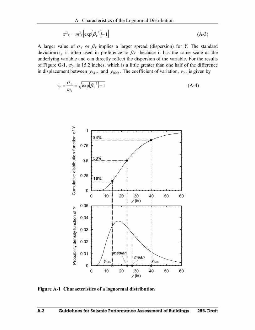
A. Characteristics of the Lognormal Distribution
A-2 Guidelines for Seismic Performance Assessment of Buildings 25% Draft
( )[ ]1exp 222 −= YYY m βσ (A-3)
A larger value of Yσ or βY implies a larger spread (dispersion) for Y. The standard deviation Yσ is often used in preference to βY because it has the same scale as the underlying variable and can directly reflect the dispersion of the variable. For the results of Figure G-1, Yσ is 15.2 inches, which is a little greater than one half of the difference in displacement between 84thy and 16thy . The coefficient of variation, Yν , is given by
( ) 1exp 2 −== YY
YY m
v βσ (A-4)
0 10 20 30 40 50 60y (in)
0
0.01
0.02
0.03
0.04
0.05
Pro
babi
lity
dens
ity fu
nctio
n of
Y
0 10 20 30 40 50 60y (in)
0
0.25
0.5
0.75
1
Cum
ulat
ive
dist
ribut
ion
func
tion
of Y
16%
84%
50%
y16th y84th
medianmean
Figure A-1 Characteristics of a lognormal distribution
25% Draft Guidelines for Seismic Performance Assessment of Buildings B-1
Appendix B Performance Groups, Damage States, and Fragilities
B.1 General
In order to simplify the assessment of building performance, each building is parsed into groups of compenents and systems that have similar damageability characteristics. These groups of components are termed performance groups. Performance groups will generally be comprised of components/systems that have the following characteristics:
• Are located in proximity to each other, such that demands imposed on all members of the group will be essentially the same.
• Have damage that is predicted by the same demand parameter, for example, interstory drift in a given direction of building resopnse, floor acceleration at a level in a given direction, or similar parameter
• Have similar consequences of damage, for example, can be repaired while the buidling remans occupied, poses a potential threat to personnel safety, etc.
Generally, structural components/systems and nonstuctural components/systems will be placed in different performance groups as damage to strucural components/systems typically has consequences with regard to potential collapse and post-earthquake occupancy restrictions, while damage to nosntructural components may not. Typically the components and systems at each floor level will be independently grouped and components that are sensitive to building motion in one direction as opposed to any direction will be separately grouped.
This Appendex provides general guidelines for formation of performance groups when the default performance groups contained in Appendix G and H are not adequate. Section D.2, below presents a general strategy for the formation of performance groups. Section D.3 describes the process for identifying appropriate damage states for each performance group.
B.2 General Strategy
A general strategy for grouping components is as follows:
a) Components that are inherently rugged and not subject to significant damage for credible levels of demand need not be considered. For example, in the example building the foundations would not be damaged since the steel moment frames are not strong enough to force inelastic behavior into the footings. Also, some components (e.g. toilet fixtures) can often be neglected as they cannot credibly be damaged.
b) Each component, for which direct damage is to be monitored, should be included in one, and only one group. Direct damage is that caused by the demand of the seismic shaking itself. Some components may not be damaged

B. Performance Groups, Damage States, and Fragilities
B-2 Guidelines for Seismic Performance Assessment of Buildings 25% Draft
directly, but can be affected by the repair of other components. For example, if a structural moment frame connection is directly damaged, repair may require the removal of some wallboard for construction access, even though the wallboard itself was not damaged.
c. Components should be grouped similarly to normal groups used for design and construction. In the example, the exterior cladding consists of the precast panels, glazing, and storefront window and door system. These items have a both a design and construction relationship that leads to a logical association for monitoring damage. If the design or construction of one is changed, the change will likely affect all. Similarly, repair of damage for one is likely to involve others.
d. Damage for each component within a performance group must be predictable by a single demand parameter for the entire group. In the example, ceilings, fire-sprinklers, and light fixtures are grouped together and damage to each is related to floor acceleration at the same building level. In some cases this implies a compromise using a demand parameter for the group that might not be the absolute best for one or more components.
e. Each performance group should generally include items at only a single floor or story level as the demands (accelerations and interstory drifts) experienced at each level of a building will typically be different. If components are sensitive to building movement in one direction, but not another, additional performance groups should be designated to recognize the directionality of the demand sensitivity.
f. The damage characteristics of all components in a performance group should be such that group damage states and fragility are logical for monitoring casualty, repair and downtime consequences of damage. The group damage states are discussed below in Section 3.5.2. In the example application, the interior partitions and exterior cladding at each floor level are sensitive to drift, yet they are placed in different performance groups because the damage states could not be logically combined while maintaining a reasonable fragility relationship.
g. More than one performance group may utilize a single demand parameter. In the example, sixteen performance groups utilize only seven different demand parameters (i.e. peak inter-story peak acceleration at each floor and roof, and peak acceleration at the ground.
B.3 Damage States and Fragilities
As described in Chapter 3, each performance group must be assigned a series of damage states. Each damage state will represent a discrete increment in the probable consequences of the damage. As an example, Table B-1 presents potential damage states for exterior glazing, a potential performance group.
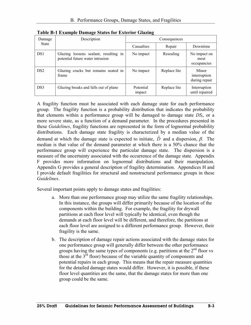
B. Performance Groups, Damage States, and Fragilities
25% Draft Guidelines for Seismic Performance Assessment of Buildings B-3
Table B-1 Example Damage States for Exterior Glazing Consequences Damage
State Description
Casualties Repair Downtime
DS1 Glazing loosens sealant, resulting in potential future water intrusion
No impact Resealing No impact on most
occupancies
DS2 Glazing cracks but remains seated in frame
No impact Replace lite Minor interruption during repair
DS3 Glazing breaks and falls out of plane Potential impact
Replace lite Interruption until repaired
A fragility function must be associated with each damage state for each performance group. The fragility function is a probability distribution that indicates the probability that elements within a performance group will be damaged to damage state DSi, or a more severe state, as a function of a demand parameter. In the procedures presented in these Guidelines, fragility functions are represented in the form of lognormal probability distributions. Each damage state fragility is characterized by a median value of the demand at which the damage state is expected to initiate, D and a dispersion, β. The median is that value of the demand parameter at which there is a 50% chance that the performance group will experience the particular damage state. The dispersion is a measure of the uncertainty associated with the occurrence of the damage state. Appendix F provides more information on lognormal distributions and their manipulation. Appendix G provides a general description of fragility determination. Appendices H and I provide default fragilities for structural and nonstructural performance groups in these Guidelines.
Several important points apply to damage states and fragilities:
a. More than one performance group may utilize the same fragility relationships. In this instance, the groups will differ primarily because of the location of the components within the building. For example, the fragility for drywall partitions at each floor level will typically be identical, even though the demands at each floor level will be different, and therefore, the partitions at each floor level are assigned to a different performance group. However, their fragility is the same.
b. The description of damage repair actions associated with the damage states for one performance group will generally differ between the other performance groups having the same types of components (e.g. partitions at the 2nd floor vs those at the 3rd floor) because of the variable quantity of components and potential repairs in each group. This means that the repair measure quantities for the detailed damage states would differ. However, it is possible, if these floor level quantities are the same, that the damage states for more than one group could be the same.

B. Performance Groups, Damage States, and Fragilities
B-4 Guidelines for Seismic Performance Assessment of Buildings 25% Draft
c. The repair measures used to define damage states are generally not unique to a single performance group nor to a single damage state. In the example, the same repair measures occur in a number of different groups and damage states.

25% Draft Guidelines for Seismic Performance Assessment of Buildings C-1
Appendix C Developing Fragility Functions for Structural and Nonstructural Components
C.1 Purpose
This appendix describes the process used to develop fragility functions for structural and nonstructural components based on laboratory testing. These fragility functions are used to assess the seismic performance of a building containing a number of structural and nonstructural components as part of the performance-based seismic design process.
C.2 Background
Seismic fragility functions are mathematical expressions that indicate the conditional probability that a component or system will experience damage equal to or more severe than a particular level, given that it experiences earthquake-induced demands of a particular severity. The severity of earthquake demands can be expressed in the form of maximum imposed displacements, velocities, accelerations, forces, inelastic deformations or a combination of these parameters. Fragility functions typically are expressed in the form:
[ ]zEDPDSDPzg iDSi =≥=)( (C-1)
where:
D is the damage sustained by the component
DSi is a specific damage state, such as initiation of cracking of a partition, a piece of electrical equipment developing a short, a mechanical seal losing integrity on a pressure containing component, a beam-column connection in a steel frame fracturing, etc.
EDP is the demand
Seismic fragility functions are typically represented as lognormal functions, characterized by a median value and a dispersion. For a given damage state DSi, the median value of the demand, z, z , is that value of z at which there is a 50% probability that damage will equal or exceed the specified level. The dispersion, typically represented by the parameter β, is the standard deviation of the natural logarithm of the values of z at which damage the damage is evaluated. Figure C-1 shows a representative nonstructural component seismic fragility function. In this particular function, the median of z has a value of 1. The dispersion has a value of 0.25. As can be seen, at a shaking intensity level z=1, there is 50% probability that the component will be damaged to damage state DSi, or a more severe level. At a shaking intensity level z=0.7 there is approximately a 10% chance that the component will be damaged to DSi, or a more severe level. At a

C. Developing Fragility Functions for Structural and Nonstructural Components
C-2 Guidelines for Seismic Performance Assessment of Buildings 25% Draft
shaking intensity level z =1.4, there is approximately a 90% chance that the component will be damaged to damage state DSi, or a more severe level.
00.10.20.30.40.50.60.70.80.9
1
0 0.5 1 1.5 2
Earthquake Shaking Intensity z
Pro
babi
lity
of E
xcee
d Da
mag
e St
ate
DSi
Figure C-1 – Hypothetical nonstructural component fragility function
The variability exhibited by seismic fragility functions can be attributed to a variety of factors including:
Random variations in the character of shaking demands at a given level of severity – for example, if shaking intensity, z, is represented by the peak acceleration experienced by the component, one earthquake may reach that peak value several times during the event while other events, of similar intensity may reach that peak value only one time.
Random variation in the strength or displacement capacity of the component itself, owing to variability in the materials of its construction and the way in which the component is manufactured, installed or constructed.
Random variation in the condition of the structure or component at the time of loading. For example, a storage rack may or may not be heavily loaded with stored contents at the time an earthquake actually occurs.
Fragility functions can be established in several ways including:
Earthquake performance data – in this method, an attempt is made to investigate the performance of a number of actual installations of the component that have experienced shaking of differing intensities. If a large number of the components have been subjected to shaking of different intensities, it is possible to directly develop a distribution of the percentage of components subjected to a given intensity of shaking that have been damaged to different levels and directly construct the fragility function.

C. Developing Fragility Functions for Structural and Nonstructural Components
25% Draft Guidelines for Seismic Performance Assessment of Buildings C-3
Simulation – in this method, a mathematical model of the structure or component is developed and a simulation is performed to predict the damage sustained by the component when subjected to shaking. A large number of simulations must typically be performed to explore the effect of variation of ground motion character, manufacturing and construction quality.
Laboratory testing – in this method, a representative sample of components is subjected to testing, in the laboratory, that represents the response of the components to actual shaking. As with simulation, ideally, a large number of tests should be performed to permit exploration of the effect of variation of ground motion character, manufacturing quality and installation quality on component behavior
This appendix describes, in a general manner, the procedures that should be used to develop nonstructural component seismic fragility functions using laboratory data.
C.3 General Procedure
As indicated in the previous section, ideally, data from a large number of tests, that explore variability in shaking character, manufacturing and installation quality should be available. However, since testing is expensive, typically, data from only a limited number of tests will be available. Therefore, development of nonstructural component seismic fragility functions will typically require the application of some expert judgment to extrapolate the available data.
Development of nonstructural component seismic fragility functions should be conducted by a panel of experts. This panel should include engineers familiar with structural reliability methods and probabilistic analysis, earthquake engineering experts and engineers familiar with the manufacture, installation and function of the particular component. Researchers who performed the testing upon which the seismic fragility will be based should be participants in the panel however these researchers should not be the sole members of the panel.
Data available from the test should include a description of the components tested, the test setup, the loading applied and for each test, the various damage states observed and for each test, the loading level at which each damage state was observed to occur.
The panel should evaluate the following factors:
The extent to which the test setup represents the actual installed condition of the component in a building and the extent that the laboratory setup may result in a systematic bias in the values of the loading at which the damage occurs
The variability of the reported values for which the damage state occurs and apparent repeatability of results from test to test

C. Developing Fragility Functions for Structural and Nonstructural Components
C-4 Guidelines for Seismic Performance Assessment of Buildings 25% Draft
The insight of the researcher who performed the test as to the critical parameters that control the damageability of the component, including for example, the rigidity and strength of base anchorage or other bracing, the combined effects of multi-axial loading, whether the component is functioning at the time of the loading and other factors that appear to affect behavior. These factors should be reported together with the researcher’s insight as to the extent of the affect of each such parameter
The variability in performance of similar types of components exhibiting similar behaviors as established by other seismic fragility development efforts
Considering this data, the panel should establish values for the median and dispersion, as previously described. The median value should not be different from the median value of the reported test data unless there is specific reason to believe that the test setup resulted in identifiable bias in the results. Generally, in order to establish a reliable estimate of the variance, based on test data alone, a large number of tests (in excess of 10) will need to be performed. Lacking such data, the variance should be established on the basis of expert judgment considering the identified factors that affect behavior, an evaluation of the amount of variability possible in each of these factors, the amount that variability in each of these factors will likely affect the results and an understanding of the degree of correlation, if any, between these various factors and the performance.
When establishing these fragility parameters, the panel must bear in mind that the intent is to establish unbiased predictions of fragility that neither over-predict nor under-predict the probability that the component will experience a given level of damage at a given level of shaking. The seismic fragility function should account only for the variability inherent in the behavior of the particular type of component. Variability in other external factors that can affect the performance of the component, but which are not directly related to the component should not be included in the fragility variability. Examples of variability that should not be included in seismic fragility functions includes the following:
Uncertainty in the intensity of ground shaking
Uncertainty in the response of the supporting structure
Uncertainty in the consequences of damage of the component
The fragility parameters should be presented in a report, prepared by the panel, which includes the following:
A description of the component and the installation condition for which the fragility applies
Identification of the panel members and their qualifications
A description of the damage state(s) for which the fragilities apply, including in a qualitative manner, discussion of the consequences of this damage (for example,

C. Developing Fragility Functions for Structural and Nonstructural Components
25% Draft Guidelines for Seismic Performance Assessment of Buildings C-5
component will not function, component will leak, component must be repaired, component must be replaced, etc.)
A description of the data and factors considered by the panel
The panel’s recommendation for median and variance
C.4 Test Protocols
Recommended protocols for laboratory testing of components to determine their seismic fragility maybe found in a companion documents FEMA xxx.


25% Draft Guidelines for Seismic Performance Assessment of Buildings D-1
Appendix D Default Damage and Loss Data for Structural Systems
D.1 General
This appendix will provide default fragility and damage functions for selected structural systems including moment-resisting steel frames and light wood frame walls.
D.2 Default Damage and Loss Data for Moment-Resisting Steel Frames
D.2.1 Introduction and scope of dataset
D.2.2 Welded-flange welded web moment-resisting frames
D.2.2.1 Damage States and Fragility Functions
D.2.2.2 Loss Functions
D.2.3 Welded flange bolted web moment-resisting frames
D.2.3.1 Damage States and Fragility Functions
D.2.3.2 Loss Functions
D.2.4 Bolted flange bolted web moment-resisting frames
D.2.4.1 Damage States and Fragility Functions
D.2.4.2 Loss Functions
D.3 Default Damage and Loss Data for Light Wood Frame Systems
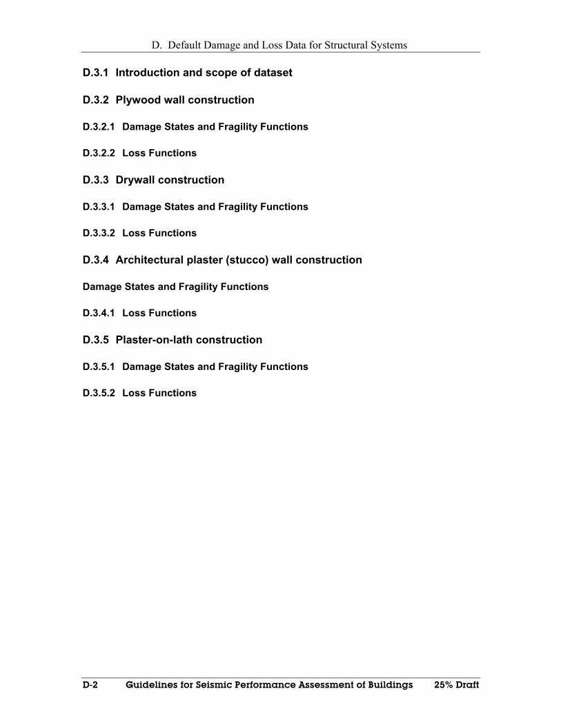
D. Default Damage and Loss Data for Structural Systems
D-2 Guidelines for Seismic Performance Assessment of Buildings 25% Draft
D.3.1 Introduction and scope of dataset
D.3.2 Plywood wall construction
D.3.2.1 Damage States and Fragility Functions
D.3.2.2 Loss Functions
D.3.3 Drywall construction
D.3.3.1 Damage States and Fragility Functions
D.3.3.2 Loss Functions
D.3.4 Architectural plaster (stucco) wall construction
Damage States and Fragility Functions
D.3.4.1 Loss Functions
D.3.5 Plaster-on-lath construction
D.3.5.1 Damage States and Fragility Functions
D.3.5.2 Loss Functions
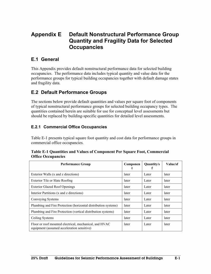
25% Draft Guidelines for Seismic Performance Assessment of Buildings E-1
Appendix E Default Nonstructural Performance Group Quantity and Fragility Data for Selected Occupancies
E.1 General
This Appendix provides default nonstructural performance data for selected building occupancies. The performance data includes typical quantity and value data for the performance groups for typical building occupancies together with default damage states and fragility data.
E.2 Default Performance Groups
The sections below provide default quantities and values per square foot of components of typical nonstructural performance groups for selected building occupancy types. The quantities contained herein are suitable for use for conceptual level assessments but should be replaced by building-specific quantities for detailed level assessments.
E.2.1 Commercial Office Occupancies
Table E-1 presents typical square foot quantity and cost data for performance groups in commercial office occupancies.
Table E-1 Quantities and Values of Component Per Square Foot, Commercial Office Occupancies
Performance Group Component
Quantity/sf
Value/sf
Exterior Walls (x and z directions) later Later later
Exterior Tile or Slate Roofing later Later later
Exterior Glazed Roof Openings later Later later
Interior Partitions (x and z directions) later Later later
Conveying Systems later Later later
Plumbing and Fire Protection (horizontal distribution systems) later Later later
Plumbing and Fire Protection (vertical distribution systems) later Later later
Ceiling Systems later Later later
Floor or roof mounted electrical, mechanical, and HVAC equipment (assumed acceleration sensitive)
later Later later
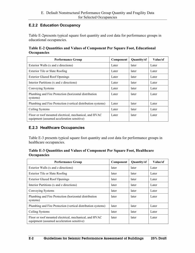
E. Default Nonstructural Performance Group Quantity and Fragility Data for Selected Occupancies
E-2 Guidelines for Seismic Performance Assessment of Buildings 25% Draft
E.2.2 Education Occupancy
Table E-2presents typical square foot quantity and cost data for performance groups in educational occupancies.
Table E-2 Quantities and Values of Component Per Square Foot, Educational Occupancies
Performance Group Component Quantity/sf Value/sf
Exterior Walls (x and z directions) Later later Later
Exterior Tile or Slate Roofing Later later Later
Exterior Glazed Roof Openings Later later Later
Interior Partitions (x and z directions) Later later Later
Conveying Systems Later later Later
Plumbing and Fire Protection (horizontal distribution systems)
Later later Later
Plumbing and Fire Protection (vertical distribution systems) Later later Later
Ceiling Systems Later later Later
Floor or roof mounted electrical, mechanical, and HVAC equipment (assumed acceleration sensitive)
Later later Later
E.2.3 Healthcare Occupancies
Table E-3 presents typical square foot quantity and cost data for performance groups in healthcare occupancies.
Table E-3 Quantities and Values of Component Per Square Foot, Healthcare Occupancies
Performance Group Component Quantity/sf Value/sf
Exterior Walls (x and z directions) later later Later
Exterior Tile or Slate Roofing later later Later
Exterior Glazed Roof Openings later later Later
Interior Partitions (x and z directions) later later Later
Conveying Systems later later Later
Plumbing and Fire Protection (horizontal distribution systems)
later later Later
Plumbing and Fire Protection (vertical distribution systems) later later Later
Ceiling Systems later later Later
Floor or roof mounted electrical, mechanical, and HVAC equipment (assumed acceleration sensitive)
later later Later

E. Default Nonstructural Performance Group Quantity and Fragility Data for Selected Occupancies
25% Draft Guidelines for Seismic Performance Assessment of Buildings E-3
E.2.4 Hospitality Occupancies
Table E-4 presents typical square foot quantity and cost data for performance groups in hospitality occupancies.
Table E-4 Quantities and Values of Component Per Square Foot, Hospitality Occupancies
Performance Group Component Quantity/sf Value/sf
Exterior Walls (x and z directions) later later Later
Exterior Tile or Slate Roofing later later Later
Exterior Glazed Roof Openings later later Later
Interior Partitions (x and z directions) later later Later
Conveying Systems later later Later
Plumbing and Fire Protection (horizontal distribution systems)
later later Later
Plumbing and Fire Protection (vertical distribution systems) later later Later
Ceiling Systems later later Later
Floor or roof mounted electrical, mechanical, and HVAC equipment (assumed acceleration sensitive)
later later Later
E.2.5 Residential Occupancies
Table E-5 presents typical square foot quantity and cost data for performance groups in residential occupancies.
Table E-5 Quantities and Values of Component Per Square Foot, Residential Occupancies
Performance Group Component Quantity/sf Value/sf
Exterior Walls (x and z directions) later later Later
Exterior Tile or Slate Roofing later later Later
Exterior Glazed Roof Openings later later Later
Interior Partitions (x and z directions) later later Later
Conveying Systems later later Later
Plumbing and Fire Protection (horizontal distribution systems)
later later Later
Plumbing and Fire Protection (vertical distribution systems) later later Later
Ceiling Systems later later Later
Floor or roof mounted electrical, mechanical, and HVAC equipment (assumed acceleration sensitive)
later later Later

E. Default Nonstructural Performance Group Quantity and Fragility Data for Selected Occupancies
E-4 Guidelines for Seismic Performance Assessment of Buildings 25% Draft
E.2.6 Research Occupancies
Table E-6 presents typical square foot quantity and cost data for performance groups in research occupancies.
Table E-6 Quantities and Values of Component Per Square Foot, Research Occupancies
Performance Group Component Quantity/sf Value/sf
Exterior Walls (x and z directions) later later Later
Exterior Tile or Slate Roofing later later Later
Exterior Glazed Roof Openings later later Later
Interior Partitions (x and z directions) later later Later
Conveying Systems later later Later
Plumbing and Fire Protection (horizontal distribution systems)
later later Later
Plumbing and Fire Protection (vertical distribution systems) later later Later
Ceiling Systems later later Later
Floor or roof mounted electrical, mechanical, and HVAC equipment (assumed acceleration sensitive)
later later Later
E.2.7 Retail Occupancies
Table E-7 presents typical square foot quantity and cost data for performance groups in retail occupancies.
Table E-7 Quantities and Values of Component Per Square Foot, Retail Occupancies
Performance Group Component Quantity/sf Value/sf
Exterior Walls (x and z directions) Later later Later
Exterior Tile or Slate Roofing Later later Later
Exterior Glazed Roof Openings Later later Later
Interior Partitions (x and z directions) Later later Later
Conveying Systems Later later Later
Plumbing and Fire Protection (horizontal distribution systems)
Later later Later
Plumbing and Fire Protection (vertical distribution systems) Later later Later
Ceiling Systems Later later Later
Floor or roof mounted electrical, mechanical, and HVAC equipment (assumed acceleration sensitive)
Later later Later

E. Default Nonstructural Performance Group Quantity and Fragility Data for Selected Occupancies
25% Draft Guidelines for Seismic Performance Assessment of Buildings E-5
E.2.8 Warehouse Occupancies
Table E-8 presents typical square foot quantity and cost data for performance groups in warehouse occupancies.
Table E-8 Quantities and Values of Component Per Square Foot, Warehouse Occupancies
Performance Group Component Quantity/sf Value/sf
Exterior Walls (x and z directions) Later Later Later
Exterior Tile or Slate Roofing Later Later Later
Exterior Glazed Roof Openings Later Later Later
Interior Partitions (x and z directions) Later Later Later
Conveying Systems Later later Later
Plumbing and Fire Protection (horizontal distribution systems)
Later later Later
Plumbing and Fire Protection (vertical distribution systems) Later later Later
Ceiling Systems Later later Later
Floor or roof mounted electrical, mechanical, and HVAC equipment (assumed acceleration sensitive)
Later later Later
E.3 Default Performance Group Fragilities
E.3.1 Basic default nonstructural component fragility data
Table E-9 provides fragility median and dispersion values for the default nonstructural performance groups.
Table E-9 Fragility Data for Default Nonstructural Performance Groups
Architectural and MEP Performance Groups
Damage State
Demand Type Median Dispersion
Exterior Walls (x and z directions) (later) Drift (later) (later)
Exterior Tile or Slate Roofing (later) Peak Horiz. Roof Accel.
(later) (later)
Exterior Glazed Roof Openings (later) Peak Vert.
Roof Accel.
(later) (later)
Interior Partitions (x and z directions) (later) Drift (later) (later)
Conveying Systems (later) Drift and Peak Horiz. Accel.
(later) (later)
Plumbing and Fire Protection (horizontal distribution systems)
(later) Peak Horiz. Floor Accel.
(later) (later)
Plumbing and Fire Protection (vertical (later) Drift (later) (later)

E. Default Nonstructural Performance Group Quantity and Fragility Data for Selected Occupancies
E-6 Guidelines for Seismic Performance Assessment of Buildings 25% Draft
distribution systems)
Ceiling Systems (later) Peak Horiz. Floor Accel.
(later) (later)
Floor or roof mounted electrical, mechanical, and HVAC equipment (assumed acceleration sensitive)
(later) Horiz. Floor Accel.
(later) (later)
E.3.2 Basic Contents Default Fragility Data
Table E-10, below, presents default fragility data for contents in various building occupancies,
Table E-10, Default contents fragility data for various building occupancies
Contents Performance Groups by Occupancy
Damage State
Demand Type Median Dispersion
Commercial Office
Desktop Computers (later) Peak Horiz. Floor Accel.
(later) (later)
Tall File Cabinets (later) Peak Vert.
Floor Accel.
(later) (later)
Tall Slender Bookcases (later) Peak Horiz. Floor Accel.
(later) (later)
Business Equipment (printers, servers, mainframes, etc.
(later) Peak Horiz. Floor Accel..
(later) (later)
Education
Bookshelves (later) Peak Horiz. Floor Accel.
(later) (later)
Desktop Computers (later) Peak Horiz. Floor Accel.
(later) (later)
Tall File Cabinets (later) Peak Horiz. Floor Accel..
(later) (later)
Healthcare/Hospitals
Medical Equipment (later) Peak Horiz. Floor Accel.
(later) (later)
Kitchen Equipment (later) Peak Vert.
Floor Accel.
(later) (later)
Tall Bookcases (later) Peak Horiz. Floor Accel.
(later) (later)
Desktop Computers (later) Peak Horiz. Floor Accel..
(later) (later)
Hospitality (Hotels/Dorms)
Kitchen Equipment (later) Peak Vert. (later) (later)

E. Default Nonstructural Performance Group Quantity and Fragility Data for Selected Occupancies
25% Draft Guidelines for Seismic Performance Assessment of Buildings E-7
Contents Performance Groups by Occupancy
Damage State
Demand Type Median Dispersion
Floor Accel.
Residential
Desktop Computers (later) Peak Horiz. Floor Accel..
(later) (later)
Home Entertainment Equipment (later) Peak Horiz. Floor Accel.
(later) (later)
China (later) Peak Vert.
Floor Accel.
(later) (later)
Research including Higher Education Labs
Retail
Storage Racks (later) Peak Horiz. Floor Accel.
(later) (later)
Tall Display Racks (later) Peak Vert.
Floor Accel.
(later) (later)
Contents on Racks (later) Peak Horiz. Floor Accel.
(later) (later)
Cold Rooms (later) Peak Horiz. Floor Accel..
(later) (later)
Warehouse
Storage Racks (later) Peak Vert.
Floor Accel.
(later) (later)
Contents on Racks (later) Peak Horiz. Floor Accel.
(later) (later)
E.3.3 Adjustment factors for contents and nonstructural components
In this section, which will be developed later, default adjustment factors will be provided which will adjust the default fragility functions provided in sections E.3.1 and E.3.2 for the factors described in Section 4.5.1, including year of installation, seismic design practice, installation quality assurance, and facility seismic safety management.
E.4 Component-Specific Fragility Data
The following list of nonstructural fragility values are taken from Porter and Kiremidjian (2001) and may be used to define fragilities for user-defined performance groups.

E. Default Nonstructural Performance Group Quantity and Fragility Data for Selected Occupancies
E-8 Guidelines for Seismic Performance Assessment of Buildings 25% Draft
Table E-11, Nonstructural Component Fragilities
Drift Sensitive Item Damage State Median Drift Dispersion
1. 5/8 in drywall partition on
3-5/8 in metal studs
Visible damage tape/paint
0.0039 0.17
Significant damage –replace
0.0085 0.23
2. Glazing Cracking 0.040 0.36
Fallout 0.046 0.33
Acceleration Sensitive Item Damage State Median Accel
Dispersion
1. Automatic Sprinklers Leaks every 1000 lf 0.55 g 0.54
Monitor fall off 3.5 0.25 2. Desktop computers
Monitor and system fall off
5.2 0.40
12 ft x 12 ft grid collapse
3.8 0.80
20 ft x 20 ft grid collapse
2.3 0.80
3. Suspended Ceiling System
40 ft x 40 ft grid collapse
1.15 0.80
4. Unanchored Elec. Cabinet Operational Failure 0.52 0.62
5. Motor Control Center Operational Failure 0.79 0.52
6. Transformer Operational Failure 1.23 0.62
7. Low voltage switchgear Operational Failure 1.12 0.64
8. Med voltage switchgear Operational Failure 1.60 0.80
9. Distribution panel Operational Failure 1.75 0.68
10. Diesel generator Operational Failure 0.87 0.51
11. Inverter Operational Failure 1.20 0.57
12. Fan Operational Failure 2.69 0.93

25% Draft Guidelines for Seismic Performance Assessment of Buildings F-1
Appendix F Constitutive Relationships for Structural Modeling
Reader Note: Appendix F is not presently developed, but will be provided in later drafts of the Guidelines.


25% Draft Guidelines for Seismic Performance Assessment of Buildings G-1
Appendix G Default Consequence Functions for Structural Systems
Reader Note: Appendix G is not presently developed, but will be provided in later drafts of the Guidelines.


25% Draft Guidelines for Seismic Performance Assessment of Buildings H-1
Appendix H Default Consequence Functions for Building Occupancies
Reader Note: Appendix H is not presently developed, but will be provided in later drafts of the Guidelines.

25% Draft Guidelines for Seismic Performance Assessment of Buildings P-1
ATC-58 Project Participants
Project Management Christopher Rojahn, Project Executive Director Applied Technology Council 201 Redwood Shores Parkway, Suite 240 Redwood City, CA 94065 650/595-1542 FAX 650/593-2320 e-mail: [email protected]
Ronald O. Hamburger, Project Technical Director Simpson Gumpertz & Heger The Landmark @ One Market, Suite 600 San Francisco, CA 94105 415/495-3700 FAX 415/495-3550 e-mail: [email protected]
FEMA Oversight Mike Mahoney, Project Officer Federal Emergency Management Agency 500 C Street, SW, Room 416 Washington, DC 20472 202/646-2794 FAX 202/646-3990 e-mail: [email protected]
Robert D. Hanson, Technical Monitor (Federal Emergency Management Agency) 2926 Saklan Indian Drive Walnut Creek, CA 94595-3911 925/946-9463 FAX 925/256-4693 e-mail: [email protected]
Project Management Committee Christopher Rojahn, Chair Ronald Hamburger, Co-Chair Peter May (University of Washington) 21817 SE 20th Street Sammamish , WA 98075 425/391-4406 FAX 425/391-0299 e-mail: [email protected] Jack P. Moehle (University of California at Berkeley) 3444 Echo Springs Road Lafayette, CA 94549 510/231-9554 FAX 510/231-9471 e-mail: [email protected]
Maryann T. Phipps* Estructure 8331 Kent Court, Suite 100 El Cerrito, CA 94530 510/235-3116 FAX 510/235-3992 e-mail: [email protected] Jon Traw Traw Associates Consulting 14435 Eastridge Drive Whittier, CA 90602 562/789-7583 FAX 562/789-7583 e-mail: [email protected]
*ATC Board Contact

ATC-58 Project Participants
P-2 Guidelines for Seismic Performance Assessment of Buildings 25% Draft
Steering Committee William T. Holmes (Chair) Rutherford & Chekene 427 Thirteenth Street Oakland, CA 94612 510/740-3200 FAX 510/740-3340 e-mail: [email protected] Dan Abrams Mid-America Earthquake Center University of Illinois 1245 Newmark Civil Engineering Lab 205 N. Mathews Urbana, IL 61801 217/333-0565 FAX 217/333-3821 e-mail: [email protected] Deborah B. Beck Beck Creative Strategies LLC 531 Main Street, Suite 313 New York, NY 10044 212/223-0030 FAX 212/486-9272 e-mail: [email protected] Randall Berdine Fannie Mae 3900 Wisconsin Avenue, NW Washington, DC 20016-2892 301/204-8043 FAX 301/280-2047 e-mail: [email protected] Roger D. Borcherdt U.S. Geological Survey 345 Middlefield Road, MS977 Menlo Park, CA 94025 650/329-5619 FAX 650/329-5163 e-mail: [email protected] Jimmy Brothers City of Decatur, Building Department 402 Lee Street NE, 4th Fl., City Hall Tower Decatur, AL 35601 256/351-7584 FAX 256/351-7581 e-mail: [email protected]
Michel Bruneau MCEER, University at Buffalo 105 Red Jacket Quadrangle Buffalo, NY 14261-0025 716/645-2114x2403 FAX 716/645-3399 e-mail: [email protected] Terry Dooley Morley Builders 2901 28th Street, Suite 100 Santa Monica, CA 90405 310/566-9265 FAX 310/314-7347 e-mail: [email protected] Mohammed Ettouney Weidlinger Associates, Inc. 375 Hudson Street New York, NY 10014-3656 212/367-3080 FAX 212/367-3030 e-mail: [email protected] John Gillengerten Office of Statewide Health
Planning and Development 1600 9th St., Room 420 Sacramento, CA 95814 916/654-3547 FAX 916/654-2973 e-mail: [email protected] William J. Petak University of Southern California School of Policy Planning and Development Lewis Hall 214, 650 Childs Way Los Angeles, CA 90089-0626 213/740-4059 FAX 213/740-5943 e-mail: [email protected] Randy Schreitmueller FM Global 1301 Atwood Avenue Johnston, RI 02919 401/275-3000 FAX 401/275-3029 e-mail: [email protected]
ATC-58 Project Participants
25% Draft Guidelines for Seismic Performance Assessment of Buildings P-3
Steering Committee (continued) Jim W. Sealy, Architect 1320 Prudential Drive, No 101 Dallas, TX 75235-4117 214/637-3047 FAX 214/637-3229 e-mail: [email protected]
Product 1 Team Ronald L. Mayes, Team Leader Simpson Gumpertz & Heger 222 Sutter Street San Francisco, CA 94108 415/495-3700x219 FAX 415/495-3550 e-mail: [email protected] Daniel Alesch (University of Wisconsin) 909 Forest Hill Drive Green Bay, WI 54311-5927 920/468-0132 FAX 920/465-2791 e-mail: [email protected]
Bruce R. Ellingwood Georgia Institute of Technology 790 Atlantic Drive Atlanta, GA 30332-0355 404/894-2202 FAX 404/894-2278 e-mail: [email protected] James O. Malley Degenkolb Engineers 225 Bush Street, Suite 1000 San Francisco, CA 94104 415/392-6952 FAX 415/981-3157 e-mail: [email protected]
Structural Performance Products Team Andrew S. Whittaker, Team Leader University at Buffalo Dept. of Civil Engineering 230 Ketter Hall Buffalo, NY 14260 716/645-2114x2418 FAX 716/645-3733 e-mail: [email protected] Gregory Deierlein Stanford University Dept. of Civil & Environmental Engrg 240 Terman Engineering Center Stanford, CA 94305-4020 650/723-0453 FAX 650/723-7514 e-mail: [email protected] Andre Filiatrault MCEER, University at Buffalo 105 Red Jacket Quadrangle Buffalo, NY 14261-0025 716/645-2114x2434 FAX 716/645-3733 e-mail: [email protected]
John Hooper Magnusson Klemencic Associates 1301 Fifth Avenue, Suite 3200 Seattle, WA 98101 206/292-1200 FAX 206/292-1201 e-mail: [email protected] Andrew T. Merovich A. T. Merovich & Associates, Inc. 1950 Addison Street, Suite 205 Berkeley, CA 94704 510/845-6600 FAX 510/845-5220 e-mail: [email protected]

ATC-58 Project Participants
P-4 Guidelines for Seismic Performance Assessment of Buildings 25% Draft
Nonstructural Performance Products Team Robert Bachman, Team Leader Consulting Structural Engineer 25152 La Estrada Drive Laguna Niguel, CA 92677 949/495-4726, Cell 916/201-7527 e-mail: [email protected] David Bonowitz Office of Court Construction & Mgmt. Judicial Council of California Administrative Office of the Courts 455 Golden Gate Avenue San Francisco, CA 94102-3688 415/865-8034 FAX 415/865-8885 e-mail: [email protected] Philip J. Caldwell Square D Company 1990 Sandifer Blvd. Seneca, SC 29687 864/886-1471 FAX 864/886-1390 e-mail: [email protected] Andre Filiatrault MCEER, University at Buffalo 105 Red Jacket Quadrangle Buffalo, NY 14261-0025 716/645-2114x2434 FAX 716/645-3733 e-mail: [email protected]
Robert P. Kennedy RPK Structural Mechanics Consulting, Inc. 28625 Mountain Meadow Road Escondido, CA 92026 760/751-3510 FAX 760/751-3537 e-mail: [email protected] Gary McGavin McGavin Architecture 447 LaVerne Street Redlands, CA 92373-6015 909/748-0014 FAX 909/748-0024 e-mail: [email protected] Eduardo Miranda Stanford University Civil & Environmental Engineering Terman Room 293 Stanford, CA 94305-3707 650/723-4450 FAX 650/725-6014 e-mail: [email protected] Keith Porter Consulting Engineer 769 N. Michigan Avenue Pasadena, CA 91104 626/395-4141 FAX 419/828-6734 e-mail: [email protected]
ATC-58 Project Participants
25% Draft Guidelines for Seismic Performance Assessment of Buildings P-5
Shaketable Testing Protocol Team Andre Filiatrault, Team Leader MCEER, University at Buffalo 105 Red Jacket Quadrangle Buffalo, NY 14261-0025 716/645-2114x2434 FAX 716/645-3733 e-mail: [email protected] Philip J. Caldwell Square D Company 1990 Sandifer Blvd. Seneca, SC 29687 864/886-1471 FAX 864/886-1390 e-mail: [email protected] Peter Dusicka Portland State University Dept. of Civil & Environmental Engineering P.O. Box 751 Portland, OR 97207-0751 503/725-9558 FAX 503/725-5950 e-mail: [email protected] Tara Hutchinson University of California, Irvine Dept. of Civil & Environmental Engineering 4130 Engineering Gateway Irvine, CA 92697 949/824-2166 FAX 949/824-2117 e-mail: [email protected] Ahmad Itani University of Nevada, Reno Dept. of Civil Engineering Mail Stop 258 Reno, NV 89557-0152 775/ 784-4379 FAX 775/784-1390 e-mail: [email protected]
Eduardo Miranda Stanford University Civil & Environmental Engineering Terman Room 293 Stanford, CA 94305-3707 650/723-4450 FAX 650/725-6014 e-mail: [email protected] Gokhan Pekcan University of Nevada, Reno Dept. of Civil Engineering Mail Stop 258 Reno, NV 89557-0152 775/784-4512 FAX 775/784-1390 e-mail: [email protected] Andrei M. Reinhorn University at Buffalo Dept. of Civil Engineering 231 Ketter Hall Buffalo, NY 14260 716/645-2114x2419 FAX 716/645-3733 e-mail: [email protected] Jose Restrepo University of California, San Diego 9500 Gillman Drive La Jolla, CA 92093-0085 858/822-3392 FAX 858/822-2260 e-mail: [email protected]

ATC-58 Project Participants
P-6 Guidelines for Seismic Performance Assessment of Buildings 25% Draft
Racking Testing Protocol Team Helmut Krawinkler, Team Leader Stanford University Civil Engineering Department Stanford, CA 94305-4020 650/723-4129 FAX 650/723-7514 e-mail: [email protected] David Bonowitz Office of Court Construction & Mgmt. Judicial Council of California Administrative Office of the Courts 455 Golden Gate Avenue San Francisco, CA 94102-3688 415/865-8034 FAX 415/865-8885 e-mail: [email protected] Barry J. Goodno Georgia Institute of Technology 790 Atlantic Drive Atlanta, GA 30332-0355 404/894-2227 FAX 404/894-2283 e-mail: [email protected] Steven Kuan Public Works Govt. Svs Canada 641-800 Burrard Street Vancouver, BC V6Z 2V8 Canada 604/775-6663 FAX 604/775-6647 e-mail: [email protected]
Joseph R. Maffei Consulting Structural Engineer 427 Thirteenth Street Oakland, CA 94612 510/740-3217 FAX 510/740-3340 e-mail: [email protected] Ali M. Memari Pennsylvania State University Dept. of Architectural Engineering 104 Engineering Unit A University Park, PA 16802-1416 814/865-6394 FAX 814/863-4789 e-mail: [email protected] Jose Restrepo University of California, San Diego 9500 Gillman Drive La Jolla, CA 92093-0085 858/822-3392 FAX 858/822-2260 e-mail: [email protected] Chia-Ming Uang University of California, San Diego 409 University Center La Jolla, CA 92093-0085 858/534-9880 FAX 858/534-6373 e-mail: [email protected]
Component Cyclic Testing Protocol Team
Manos Maragakis, Team Leader University of Nevada, Reno Dept. of Civil Engineering Mail Stop 258 Reno, NV 89557-0152 775/784-6937 FAX 775/784-1390 e-mail: [email protected] George Antaki Westinghouse Savannah River Company Savannah River Site, Building 730-1B/214 Aiken, SC 29808 803/952-9728 FAX 803/952-7293 e-mail: [email protected]
Scott Campbell Kinetics Noise Control 6300 Frelan Place Dublin, OH 43017 614/889-0480 FAX 614/889-0540 e-mail: [email protected] Robert Kennedy RPK Structural Mechanics Consulting, Inc. 28625 Mountain Meadow Road Escondido, CA 92026 760/751-3510 FAX 760/751-3537 e-mail: [email protected]
ATC-58 Project Participants
25% Draft Guidelines for Seismic Performance Assessment of Buildings P-7
Component Cyclic Testing Protocol Team (continued) Praveen Malhotra FM Global Research 1151 Boston-Providence Turnpike Norwood, MA 02062 781/255-4931 FAX 781/255-4024 e-mail: [email protected] Sami Masri University of Southern California Dept. of Civil Engineering Los Angeles, CA 90089-2531 213/740-0602 FAX 213/744-1426 e-mail: [email protected]
John F. Silva Hilti Inc. 84 Mt. Rainier Drive San Rafael, CA 94903 415/507-1690 FAX 415/507-1695 e-mail: [email protected]
Risk Management Products Team Craig D. Comartin, Team Leader Comartin Engineers 7683 Andrea Avenue Stockton, CA 95207-1705 209/472-1221; Fax, 209/472-7294 e-mail: [email protected] Brian J. Meacham, Team Associate Leader Arup 1500 West Park Drive, Suite 180 Westborough, MA 01581 508/616-9990 FAX 508/616-9991 e-mail: [email protected] C. Allin Cornell (Stanford University) 110 Coquito Way Portola Valley, CA 94028-7404 650/854-8053 FAX 650/854-8075 e-mail: [email protected]
Gee Heckscher Architectural Resources Group Pier 9 The Embarcadero San Francisco, CA 94111 415/421-1680x216 FAX 415/421-0127 e-mail: [email protected] Charles Kircher Kircher & Associates, Consulting Engineers 1121 San Antonio Road, Suite D-202 Palo Alto, CA 94303-4311 650/968-3939 FAX 650/968-0960 e-mail: [email protected] Robert D. Weber R.D. Weber & Associates, Inc. 9784 Ice Box Canyon Court Las Vegas, NV 89117 702/838-6073 FAX 702/838-6081 e-mail: [email protected]