Seismic Fragility Analysis of Equipment and Structures in ...

2 0 1 3
Editor: Amir M. Kaynia Reviewer: Iunio Iervolino
Publishing Editors: Fabio Taucer and Ufuk Hancilar
SYNER-G Reference Report 4
Guidelines for deriving seismic fragility
functions of elements at risk:
Buildings, lifelines, transportation
networks and critical facilities
Report EUR 25880 EN

European Commission
Joint Research Centre
Institute for the Protection and Security of the Citizen
Contact information
Fabio Taucer
Address: Joint Research Centre, Via Enrico Fermi 2749, TP 480, 21027 Ispra (VA), Italy
E-mail: [email protected]
Tel.: +39 0332 78 5886
Fax: +39 0332 78 9049
http://elsa.jrc.ec.europa.eu/
http://www.jrc.ec.europa.eu/
Legal Notice
Neither the European Commission nor any person acting on behalf of the Commission
is responsible for the use which might be made of this publication.
Europe Direct is a service to help you find answers to your questions about the European Union
Freephone number (*): 00 800 6 7 8 9 10 11
(*) Certain mobile telephone operators do not allow access to 00 800 numbers or these calls may be billed.
A great deal of additional information on the European Union is available on the Internet.
It can be accessed through the Europa server http://europa.eu/.
JRC80561
EUR 25880 EN
ISBN 978-92-79-28966-8
ISSN 1831-9424
doi: 10.2788/19605
Luxembourg: Publications Office of the European Union, 2013
© European Union, 2013
Reproduction is authorised provided the source is acknowledged.
Printed in Ispra (Va) - Italy
D 8.10 DELIVERABLE
PROJECT INFORMATION
Project Title: Systemic Seismic Vulnerability and Risk Analysis for Buildings, Lifeline Networks and Infrastructures Safety Gain
Acronym: SYNER-G
Project N°: 244061
Call N°: FP7-ENV-2009-1
Project start: 01 November 2009
Duration: 36 months
DELIVERABLE INFORMATION
Deliverable Title: D8.10 - Guidelines for deriving seismic fragility functions of elements at risk: Buildings, lifelines, transportation networks and critical facilities
Date of issue: 31 March 2013
Work Package: WP8 – Guidelines, recommendations and dissemination
Deliverable/Task Leader: Joint Research Centre
Editor: Amir M. Kaynia (NGI)
Reviewer: Iunio Iervolino (AMRA)
REVISION: Final
Project Coordinator: Institution:
e-mail: fax:
telephone:
Prof. Kyriazis Pitilakis Aristotle University of Thessaloniki [email protected] + 30 2310 995619 + 30 2310 995693

The SYNER-G Consortium
Aristotle University of Thessaloniki (Co-ordinator) (AUTH)
Vienna Consulting Engineers (VCE)
Bureau de Recherches Geologiques et Minieres (BRGM)
European Commission – Joint Research Centre (JRC)
Norwegian Geotechnical Institute (NGI)
University of Pavia (UPAV)
University of Roma “La Sapienza” (UROMA)
Middle East Technical University (METU)
Analysis and Monitoring of Environmental Risks (AMRA)
University of Karlsruhe (KIT-U)
University of Patras (UPAT)
Willis Group Holdings (WILLIS)
Mid-America Earthquake Center, University of Illinois (UILLINOIS)
Kobe University (UKOBE)

i
Foreword
SYNER-G is a European collaborative research project funded by European Commission (Seventh Framework Program, Theme 6: Environment) under Grant Agreement no. 244061. The primary purpose of SYNER-G is to develop an integrated methodology for the systemic seismic vulnerability and risk analysis of buildings, transportation and utility networks and critical facilities, considering for the interactions between different components and systems. The whole methodology is implemented in an open source software tool and is validated in selected case studies. The research consortium relies on the active participation of twelve entities from Europe, one from USA and one from Japan. The consortium includes partners from the consulting and the insurance industry.
SYNER-G developed an innovative methodological framework for the assessment of physical as well as socio-economic seismic vulnerability and risk at the urban/regional level. The built environment is modelled according to a detailed taxonomy, grouped into the following categories: buildings, transportation and utility networks, and critical facilities. Each category may have several types of components and systems. The framework encompasses in an integrated fashion all aspects in the chain, from hazard to the vulnerability assessment of components and systems and to the socio-economic impacts of an earthquake, accounting for all relevant uncertainties within an efficient quantitative simulation scheme, and modelling interactions between the multiple component systems.
The methodology and software tools are validated in selected sites and systems in urban and regional scale: city of Thessaloniki (Greece), city of Vienna (Austria), harbour of Thessaloniki, gas system of L’Aquila in Italy, electric power network, roadway network and hospital facility again in Italy.
The scope of the present series of Reference Reports is to document the methods, procedures, tools and applications that have been developed in SYNER-G. The reports are intended to researchers, professionals, stakeholders as well as representatives from civil protection, insurance and industry areas involved in seismic risk assessment and management.
Prof. Kyriazis Pitilakis Aristotle University of Thessaloniki, Greece
Project Coordinator of SYNER-G
Fabio Taucer and Ufuk Hancilar Joint Research Centre
Publishing Editors of the SYNER-G Reference Reports


i


iii
Abstract
The objective of SYNER-G in regards to the fragility functions is to propose the most appropriate functions for the construction typologies in Europe. To this end, fragility curves from literature were collected, reviewed and, where possible, validated against observed damage and harmonised. In some cases these functions were modified and adapted, and in other cases new curves were developed. The most appropriate fragility functions are proposed for buildings, lifelines, transportation infrastructures and critical facilities. A software tool was also developed for the storage, harmonisation and estimation of the uncertainty of fragility functions.
Keywords: electric power system, fire-fighting system, fragility curve, gas and oil network, harbour, health-care facility, intensity measure, limit state, building, performance indicator, performance level, bridge, railway, road, taxonomy, uncertainty, water and waste water network


v
Acknowledgments
The research leading to these results has received funding from the European Community's Seventh Framework Programme [FP7/2007-2013] under grant agreement n° 244061


vii
Deliverable Contributors
AUTH Kyriazis Pitilakis Sections 1, 4.3, 5
Sotiris Argyroudis Sections 1, 4.3, 5.1, 5.3
Kalliopi Kakderi Sections 4.3, 6.2
BRGM Pierre Gehl Section 2
Nicolas Desramaut Section 4.2
KIT-U Bijan Khazai Section 1
METU Ahmet Yakut Section 3
NGI Amir M. Kaynia Sections 1, 5.1, 5.3
Jörgen Johansson Sections 5.1, 5.3
UPAT Michael Fardis Sections 3, 5.3, 7
Filitsa Karantoni Section 3
Paraskevi Askouni Section 5.3
Foteini Lyrantzaki Section 3
Alexandra Papailia Section 3
Georgios Tsionis Sections 3, 5.3, 7
UPAV Helen Crowley Sections 2, 3, 5.3
Miriam Colombi Sections 3, 5.3
Federica Bianchi Section 3
Ricardo Monteiro Section 5.3
UROMA Paolo Pinto Sections 4.1, 6.1
Paolo Franchin Sections 4.1, 6.1
Alessio Lupoi Section 6.1
Francesco Cavalieri Section 4.1
Ivo Vanzi Section 4.1


ix
Table of Contents
Foreword .................................................................................................................................... i
Abstract .................................................................................................................................... iii
Acknowledgments .................................................................................................................... v
Deliverable Contributors ........................................................................................................ vii
Table of Contents ..................................................................................................................... ix
List of Figures ......................................................................................................................... xv
List of Tables .......................................................................................................................... xxi
List of Symbols ................................................................................................................... xxvii
List of Acronyms .................................................................................................................. xxxi
1 Introduction and objectives ............................................................................................. 1
1.1 BACKGROUND .......................................................................................................... 1
1.2 DERIVATION OF FRAGILITY CURVES..................................................................... 2
1.3 TYPOLOGY ............................................................................................................... 2
1.4 PERFORMANCE LEVELS ......................................................................................... 2
1.5 INTENSITY MEASURES ............................................................................................ 3
1.6 PERFORMANCE INDICATORS ................................................................................. 4
1.7 TREATMENT OF UNCERTAINTIES .......................................................................... 4
1.8 RELATION WITH THE SOCIO-ECONOMIC LOSSES ............................................... 5
1.9 MAIN RESULTS ......................................................................................................... 5
1.10 OUTLINE AND OBJECTIVES .................................................................................... 6
2 Methods for deriving fragility functions .......................................................................... 9
2.1 INTRODUCTION ........................................................................................................ 9
2.2 EMPIRICAL METHODS ............................................................................................. 9
2.3 ANALYTICAL METHODS ......................................................................................... 10
2.3.1 Dynamic analyses ........................................................................................ 11
2.3.2 Capacity spectrum method ........................................................................... 12
2.4 EXPERT JUDGEMENT ............................................................................................ 14
2.4.1 Curves based on expert opinion ................................................................... 14
2.4.2 Macroseismic models ................................................................................... 15
2.5 HYBRID METHODS ................................................................................................. 18
3 Fragility functions for buildings .................................................................................... 19

x
3.1 REVIEW OF FRAGILITY FUNCTIONS FOR EUROPEAN BUILDINGS ................... 19
3.1.1 Definition of limit states ................................................................................. 19
3.1.2 Key elements in definition of fragility function ............................................... 21
3.1.3 Data sources ................................................................................................ 26
3.2 NEW FRAGILITY CURVES FOR RC AND MASONRY BUILDINGS ........................ 30
3.2.1 Fragility curves for RC frame and dual buildings designed according to Eurocode 2 and 8 ......................................................................................... 30
3.2.2 Fragility curves for stone masonry buildings based on FE analysis .............. 32
3.3 TAXONOMY OF EUROPEAN BUILDING TYPOLOGIES ......................................... 33
3.4 HARMONISATION OF FRAGILITY FUNCTIONS .................................................... 34
3.4.1 Harmonisation of intensity measure types .................................................... 34
3.4.2 Harmonisation of limit states ......................................................................... 35
3.4.3 Harmonisation of building typology ............................................................... 35
3.5 COMPARISON OF FRAGILITY FUNCTIONS .......................................................... 38
4 Fragility functions for utility networks .......................................................................... 43
4.1 ELECTRIC POWER NETWORK .............................................................................. 43
4.1.1 Identification of main typologies .................................................................... 43
4.1.2 State of the art fragility functions for electric power system components ...... 43
4.1.3 Proposal of standard damage scales ............................................................ 47
4.1.4 Proposed fragility functions of electric power system components for use in SYNER-G systemic vulnerability analysis ................................................. 52
4.2 GAS AND OIL NETWORKS ..................................................................................... 55
4.2.1 Identification of main typologies .................................................................... 55
4.2.2 Existing methodologies to derive fragility functions ....................................... 55
4.2.3 Damage description ..................................................................................... 58
4.2.4 State of the art fragility functions for gas and oil networks components ........ 61
4.2.5 Selection of appropriate fragility functions for European typologies .............. 65
4.2.6 Summary of the proposed fragility functions ................................................. 66
4.3 WATER AND WASTE-WATER NETWORKS ........................................................... 68
4.3.1 Identification of main typologies .................................................................... 68
4.3.2 State of art the fragility functions for water and waste-water network components .................................................................................................. 69
4.3.3 Selection of appropriate fragility functions for European typologies .............. 69
5 Fragility functions for transportation infrastructures .................................................. 73
5.1 ROADWAY AND RAILWAY BRIDGES .................................................................... 73
xi
5.1.1 Existing fragility functions for European bridges ........................................... 74
5.1.2 Development of new fragility functions ......................................................... 81
5.1.3 Taxonomy for European bridge typologies ................................................... 84
5.1.4 Harmonisation of European fragility functions ............................................... 84
5.1.5 Comparison of fragility functions ................................................................... 87
5.1.6 Closing remarks ........................................................................................... 89
5.2 ROADWAY NETWORKS ......................................................................................... 90
5.2.1 Identification of main typologies .................................................................... 90
5.2.2 Damage description ..................................................................................... 90
5.2.3 State of the art fragility functions for roadway components ........................... 91
5.2.4 Development of fragility functions by numerical analyses ............................. 94
5.2.5 Tunnels ........................................................................................................ 96
5.2.6 Embankments and trenches ......................................................................... 99
5.2.7 Bridge abutments ....................................................................................... 101
5.2.8 Slopes ........................................................................................................ 103
5.2.9 Road pavements (ground failure) ............................................................... 103
5.2.10 Summary of the proposed fragility functions ............................................... 104
5.3 RAILWAY NETWORKS .......................................................................................... 106
5.3.1 Identification of main typologies .................................................................. 106
5.3.2 Damage description ................................................................................... 106
5.3.3 Fragility functions for railway components .................................................. 107
5.3.4 Embankments, trenches and abutments..................................................... 108
5.3.5 Slopes ........................................................................................................ 109
5.3.6 Railway tracks (ground failure) ................................................................... 109
5.3.7 Summary of the proposed fragility functions ............................................... 109
5.4 HARBOUR ELEMENTS ......................................................................................... 111
5.4.1 Identification of main typologies .................................................................. 111
5.4.2 Damage description ................................................................................... 111
5.4.3 State of the art fragility functions for harbour elements components ........... 112
5.4.4 Selection of appropriate fragility functions for European typologies ............ 114
5.4.5 Summary of the proposed fragility functions ............................................... 114
6 Fragility functions for critical facilities ........................................................................ 117
6.1 HEALTH-CARE FACILITIES .................................................................................. 117
6.1.1 System components ................................................................................... 117

xii
6.1.2 The physical component ............................................................................. 118
6.1.3 Organisational component: Emergency plan .............................................. 126
6.1.4 Human component: Operators ................................................................... 127
6.1.5 Environment component ............................................................................. 127
6.1.6 Performance of hospitals under emergency conditions: Hospital Treatment Capacity ..................................................................................................... 129
6.1.7 Summary of seismic risk analysis of hospital system .................................. 130
6.2 FIRE-FIGHTING SYSTEMS ................................................................................... 132
6.2.1 Identification of main typologies .................................................................. 132
6.2.2 Damage description ................................................................................... 132
6.2.3 Fragility functions for fire-fighting systems .................................................. 132
7 Conclusions - Final remarks ........................................................................................ 133
7.1 METHODS FOR DERIVING FRAGILITY FUNCTIONS .......................................... 133
7.2 FRAGILITY FUNCTIONS FOR REINFORCED CONCRETE AND MASONRY BUILDINGS ............................................................................................................ 133
7.3 FRAGILITY FUNCTIONS FOR UTILITY NETWORKS ........................................... 134
7.4 FRAGILITY FUNCTIONS FOR TRANSPORTATION INFRASTRUCTURES ......... 134
7.5 FRAGILITY FUNCTIONS FOR CRITICAL FACILITIES .......................................... 135
7.6 FURTHER DEVELOPMENT .................................................................................. 135
References ............................................................................................................................ 137
Appendix A ............................................................................................................................ 149
A Proposed fragility curves for buildings ....................................................................... 149
A.1 RC BUILDINGS ...................................................................................................... 149
A.2 MASONRY BUILDINGS ......................................................................................... 155
Appendix B ............................................................................................................................ 159
B Proposed fragility curves for utility networks ............................................................. 159
B.1 GAS AND OIL NETWORKS ................................................................................... 159
B.1.1 Pipeline components .................................................................................. 159
B.1.2 Storage tanks ............................................................................................. 162
B.1.3 Processing facilities .................................................................................... 163
B.2 WATER SYSTEM ................................................................................................... 164
B.2.1 Water sources ............................................................................................ 164
B.2.2 Water treatment plants ............................................................................... 166
B.2.3 Pumping stations ........................................................................................ 167
B.2.4 Storage tanks ............................................................................................. 169

xiii
B.2.5 Canals ........................................................................................................ 170
B.2.6 Pipes .......................................................................................................... 171
B.2.7 Tunnels ...................................................................................................... 172
B.3 WASTE-WATER SYSTEM ..................................................................................... 172
B.3.1 Waste-water treatment plants ..................................................................... 172
B.3.2 Lift stations ................................................................................................. 174
B.3.3 Conduits ..................................................................................................... 175
Appendix C ............................................................................................................................ 177
C Proposed fragility curves for transportation infrastructures ..................................... 177
C.1 ROADWAY BRIDGES ............................................................................................ 177
C.2 ROADWAY NETWORKS ....................................................................................... 183
C.2.1 Tunnels ...................................................................................................... 183
C.2.2 Metro / urban tunnels in alluvial .................................................................. 185
C.2.3 Embankments (road on) ............................................................................. 187
C.2.4 Trenches (road in) ...................................................................................... 187
C.2.5 Bridge abutments ....................................................................................... 189
C.2.6 Slopes (road on) ......................................................................................... 190
C.2.7 Road pavements ........................................................................................ 191
C.3 RAILWAY NETWORKS .......................................................................................... 192
C.3.1 Tunnels ...................................................................................................... 192
C.3.2 Embankments (track on) ............................................................................ 192
C.3.3 Trenches (track in) ..................................................................................... 193
C.3.4 Bridge abutments ....................................................................................... 194
C.3.5 Slopes (track on) ........................................................................................ 195
C.3.6 Railway tracks ............................................................................................ 196
C.4 HARBOUR ELEMENTS ......................................................................................... 197
C.4.1 Waterfront structures .................................................................................. 197
C.4.2 Cargo handling and storage components ................................................... 199
C.4.3 Port infrastructures ..................................................................................... 201
D Proposed fragility curves for critical facilities ............................................................ 207
D.1 HEALTH-CARE FACILITIES .................................................................................. 207
D.1.1 Fragility curves for drift sensitive elements ................................................. 207
D.1.2 Fragility curves for acceleration sensitive elements .................................... 207
D.1.3 Fragility curves for architectural elements ................................................... 208

xiv
D.1.4 Fragility curves for medical gas systems .................................................... 209
D.1.5 Fragility curves for electric power systems ................................................. 209
D.1.6 Fragility curves for water systems............................................................... 209
D.1.7 Fragility curves for elevators ....................................................................... 210
xv
List of Figures
Fig. 1.1 Examples of (a) vulnerability function and (b) fragility function ................................ 1
Fig. 1.2 Screenshot of the main window of the Fragility Function Manager tool.................... 6
Fig. 2.1 Example of fragility curves built from the damage distribution on RC moment-resisting frame buildings (Orsini, 1999) ............................................................ 10
Fig. 2.2 HAZUS capacity curve and associated uncertainties (NIBS, 2004) ....................... 13
Fig. 2.3 Evolution of µD with respect to intensity, I, for different typologies of RISK-UE project (Milutinovic and Trendafilovski, 2003) ................................................... 18
Fig. 3.1 Limit States and Damage States ........................................................................... 20
Fig. 3.2 Example of a compiled fragility function review form ............................................. 26
Fig. 3.3 Pie chart exposing percentages of methodologies used to develop fragility function for reinforced concrete buildings (a) and masonry buildings (b) ....................... 27
Fig. 3.4 Pie chart exposing percentages of intensity measure types used to develop fragility function for reinforced concrete buildings (a) and masonry buildings (b) .......... 29
Fig. 3.5 Original Kappos et al. (2006a) fragility function set (a) and harmonized Kappos et al. (2006a) fragility function set (b) ................................................................... 35
Fig. 3.6 Flow chart for a reinforced concrete moment resisting frame building class - the number of available fragility functions sets is shown in the blue brackets ......... 37
Fig. 3.7 Flow chart for masonry buildings - the number of available fragility functions sets is reported in the blue brackets ............................................................................ 38
Fig. 3.8 Histogram of median values (a), histogram of dispersion values (b), correlation between median and dispersion (c) and individual and mean ± one standard deviation fragilities (d) [from Bradley (2010)] .................................................... 39
Fig. 3.9 Yield limit state (a) and collapse limit state (b) harmonised fragility functions for a reinforced concrete building typology ............................................................... 40
Fig. 3.10 Mean fragility function for (a) limit state yielding curve and (b) limit state collapse curve for a reinforced concrete building typology ............................................. 41
Fig. 3.11 Correlation between individual fragility functions parameters .............................. 41
Fig. 4.1 Decomposition of a compressor station into a fault-tree ........................................ 58
Fig. 4.2 Example of a fault-tree for an anchored steel tank (ALA, 2001) ............................. 59
Fig. 5.1 Example of fragility function review form for bridges .............................................. 78
Fig. 5.2 Original fragility function set (a) and harmonized fragility function set (b) Avsar et al. (2011) .............................................................................................................. 86
Fig. 5.3 Flowchart for reinforced concrete bridges class - the number of available fragility functions sets are shown in brackets................................................................ 86
xvi
Fig. 5.4 Minor damage state (a) and collapse damage state (b) harmonised fragility functions for reinforced concrete, isolated, regular/semi-regular bridges .......... 87
Fig. 5.5 Mean fragility function of minor damage limit state curves (a) and collapse limit state curves (b) for a reinforced concrete bridge group typology ............................... 88
Fig. 5.6 Road embankment failure caused by lateral slumping during the 1995 Kozani (GR) earthquake (left) and damage of pavement during the 2003 Lefkas (GR) earthquake caused by subsidence due to soil liquefaction (right) ..................... 91
Fig. 5.7 Proposed procedure for deriving numerical fragility curves for road elements ....... 95
Fig. 5.8 Example of evolution of damage with earthquake intensity measure and definition of threshold median value for the damage state i, and definition of standard deviation (βD) due to input motion (demand) ................................................... 96
Fig. 5.9 Example of 2D analysis results: deformed mesh (a), total moment and axial forces of the circular (b) and rectangular (c) tunnel lining (Soil profile: type B, 60m, Input motion: Kypseli, 0.3g) .............................................................................. 99
Fig. 5.10 Finite element mesh used in the analyses of embankment ................................ 100
Fig. 5.11 Properties of soil/backfill/abutment under study ................................................. 102
Fig. 5.12 Finite element mesh used in the analyses of bridge abutment .......................... 102
Fig. 5.13 Damage to railway tracks between Izimit and Arifiye due to axial strain during the 1999 Kocaeli (TR) earthquake (left) and closure of Shin-etsu line railway due to landslide during 2007 Niigata Chuetsu-Oki (JP) earthquake (right) ................ 107
Fig. 5.14 Seaward movement of quay-wall during the 2003 Tokachi-Oki earthquake (left), Turnover and extensive tilting of quay-walls during the 1995 Hyogo-ken Nanbu (Kobe) earthquake (right) ............................................................................... 112
Fig. 6.1 System taxonomy of a hospital ............................................................................ 117
Fig. 6.2 Steps in the performance assessment procedure (Lupoi et al., 2008) ................. 119
Fig. 6.3 Generic Fault-Tree for physical component ......................................................... 126
Fig. A.1 Yield limit state (a) and collapse limit state (b) harmonised fragility functions for a reinforced concrete mid-rise building with moment resisting frame ................ 149
Fig. A.2 Yield limit state (a) and collapse limit state (b) harmonised fragility functions for a reinforced concrete mid-rise building with moment resisting frame ................ 150
Fig. A.3 Yield limit state (a) and collapse limit state (b) harmonised fragility functions for a reinforced concrete mid-rise building with bare moment resisting frame with lateral load design .......................................................................................... 150
Fig. A.4 Yield limit state (a) and collapse limit state (b) harmonised fragility functions for a reinforced concrete mid-rise building with bare moment resisting frame with lateral load design .......................................................................................... 151
Fig. A.5 Mean curve for yielding limit state (a) and collapse limit state (b) for a reinforced concrete mid-rise building with moment resisting frame ................................. 151
Fig. A.6 Mean curve for yielding limit state (a) and collapse limit state (b) for reinforced concrete mid-rise building with bare moment resisting frame with lateral load design ............................................................................................................ 152
xvii
Fig. A.7 Mean curve for yielding limit state (a) and collapse limit state (b) for a reinforced concrete mid-rise building with bare moment resisting frame with lateral load design ............................................................................................................ 153
Fig. A.8 Mean curve for yielding limit state (a) and collapse limit state (b) for a reinforced concrete mid-rise building with bare non-ductile moment resisting frame with lateral load design .......................................................................................... 154
Fig. A.9 Yield limit state (a) and collapse limit state (b) harmonised fragility functions for low-rise masonry buildings ................................................................................... 155
Fig. A.10 Yield limit state (a) and collapse limit state (b) harmonised fragility functions for mid-rise masonry buildings ............................................................................ 156
Fig. A.11 Mean curve for yielding limit state (a) and collapse limit state (b) for low-rise masonry buildings .......................................................................................... 156
Fig. A.12 Mean curve for yielding limit state (a) and collapse limit state (b) for mid-rise masonry buildings .......................................................................................... 157
Fig. B.1 Proposed fragility curves for most common gas and oil pipeline typologies (ALA, 2001), for wave propagation .......................................................................... 160
Fig. B.2 Proposed fragility curves for most common gas and oil pipeline typologies (ALA, 2001), for permanent ground deformation ...................................................... 161
Fig. B.3 Fragility curves for steel tank farms (NIBS, 2004) ............................................... 162
Fig. B.4 Fragility curves for pumping / compressor plants: on left, Greek, SRMLIFE, 2003-2007) on right, generic plants (NIBS, 2004) ................................................... 163
Fig. B.5 Fragility curves for wells with anchored components in low-rise RC building with low (top) and advanced (bottom) seismic design subjected to ground shaking ..... 165
Fig. B.6 Fragility curves for water treatment plant (anchored components) subjected to ground shaking .............................................................................................. 167
Fig. B.7 Fragility curves for pumping stations with anchored components in low-rise RC building with low (up) and advanced (down) seismic design subjected to ground shaking .......................................................................................................... 167
Fig. B.8 Fragility curves for waste-water treatment plants with anchored components in low-rise RC building with low (up) and advanced (down) seismic design subjected to ground shaking .............................................................................................. 172
Fig. B.9 Fragility curves for lift stations with anchored components in low-rise RC building with low (up) and advanced (down) seismic design subjected to ground shaking ...................................................................................................................... 175
Fig. C.1 (a) Minor damage limit state and (b) Collapse limit state harmonised fragility functions for reinforced concrete, isolated pier-to-deck connection, regular/semi-regular bridges type ....................................................................................... 177
Fig. C.2 (a) Minor damage limit state and (b) Collapse limit state harmonised fragility functions for reinforced concrete, isolated pier-to-deck connection, irregular bridges type ................................................................................................... 178
xviii
Fig. C.3 (a) Minor damage limit state and (b) Collapse limit state harmonised fragility functions for reinforced concrete, non-isolated pier-to-deck connection, regular/semi-regular bridges type ................................................................... 178
Fig. C.4 (a) Minor damage limit state and (b) Collapse limit state harmonised fragility functions for reinforced concrete, non-isolated pier-to-deck connection, irregular bridges type ................................................................................................... 179
Fig. C.5 Mean and individual fragility curves for (a) minor damage limit state and (b) collapse limit state, for reinforced concrete, isolated pier-to-deck connection, regular or semi-regular bridges type............................................................... 179
Fig. C.6 Mean and individual fragility curves for (a) minor damage limit state and (b) collapse limit state, for reinforced concrete, isolated pier-to-deck connection, irregular bridges type ..................................................................................... 180
Fig. C.7 Mean and individual fragility curves for (a) minor damage limit state and (b) collapse limit state, for reinforced concrete, non-isolated pier-to-deck connection, regular or semi-regular bridges type ........................................... 181
Fig. C.8 Mean and individual fragility curves for (a) minor damage limit state and (b) collapse limit state, for reinforced concrete, non-isolated pier-to-deck connection, irregular bridges type .................................................................. 182
Fig. C.9 Fragility curves for tunnels in rock ....................................................................... 184
Fig. C.10 Fragility curves for tunnels in alluvial and cut and cover .................................... 184
Fig. C.11 Fragility curves for circular (bored) metro/urban tunnel section ......................... 186
Fig. C.12 Fragility curves for rectangular (cut and cover) metro/urban tunnel section ....... 186
Fig. C.13 Fragility curves for road embankment, h = 2 m and h = 4 m, ground type C (left) and D (right) ................................................................................................... 187
Fig. C.14 Fragility curves for road trench, ground type C (left) and D (right) ..................... 188
Fig. C.15 Fragility curves for abutment, ground type C (left) and D (right) ........................ 189
Fig. C.16 Fragility curves at various damage states and different yield coefficients (ky) for roads on slope ............................................................................................... 190
Fig. C.17 Fragility curves for road pavements subjected to ground failure ........................ 192
Fig. C.18 Fragility curves for railway embankment, h = 2 m and h = 4 m, ground type C and D .................................................................................................................... 193
Fig. C.19 Fragility curves for railway trench, ground type C (left) and D (right) ................. 194
Fig. C.20 Fragility curves for railway abutment, ground type C (left) and D (right) ............ 195
Fig. C.21 Fragility curves at various damage states and different yield coefficients (ky) for railway tracks on slope ................................................................................... 195
Fig. C.22 Fragility curves for railway tracks subjected to ground failure............................ 197
Fig. C.23 Fragility curves for waterfront structures subject to ground failure ..................... 197
Fig. C.24 Fragility curves for waterfront structures subject to ground shaking .................. 198
xix
Fig. C.25 Fragility curves for cargo handling and storage components subject to ground shaking .......................................................................................................... 200
Fig. C.26 Fragility curves for cargo handling and storage components subject to ground failure ............................................................................................................. 201
Fig. C.27 Fragility curves for fuel facilities subject to ground shaking ............................... 204
Fig. C.28 Fragility curves for fuel facilities subject to ground failure .................................. 204
Fig. C.29 Fragility curves for communication facilities ...................................................... 206
Fig. D.1 Fragility curves for drift-sensitive non-structural elements ................................... 207
Fig. D.2 Fragility curves for acceleration-sensitive non-structural elements (High-code) .. 208


xxi
List of Tables
Table 2.1 Damage state definitions (Risk-UE) .................................................................... 14
Table 2.2 Recommended values of vulnerability index for different typologies of Risk-UE project (Milutinovic and Trendafilovski, 2003) ................................................... 17
Table 2.3 Values of modification factors for RC buildings of Risk-UE project (Milutinovic and Trendafilovski, 2003) ........................................................................................ 17
Table 3.1 Comparison of existing damage scales with HRC damage scale [adapted from Rossetto and Elnashai, 2003] .......................................................................... 20
Table 3.2 List of references considered and corresponding methods for RC and masonry buildings .......................................................................................................... 27
Table 3.3 Parameters of fragility curves for RC ductile frame buildings .............................. 31
Table 3.4 Parameters of fragility curves for RC non-ductile frame buildings ....................... 31
Table 3.5 Parameters of fragility curves for RC wall buildings ............................................ 32
Table 3.6 Parameters of fragility curves for RC dual buildings ........................................... 32
Table 3.7 Median, μ, and standard deviation, β, of fragility curves for classes of stone masonry buildings ............................................................................................ 33
Table 3.8 Mean and coefficient of variation, cv, of lognormal fragility parameters for a reinforced concrete building typology ............................................................... 41
Table 3.9 Correlation coefficient matrix for a reinforced concrete building typology ............ 42
Table 4.1 Main typologies of EPN components in Europe .................................................. 44
Table 4.2 Main works on fragilities of EPN components ..................................................... 45
Table 4.3 Damage scale for electric power grids: first proposal .......................................... 47
Table 4.4 Damage scale for electric power grids: second proposal .................................... 48
Table 4.5 Damage scale for generation plants ................................................................... 48
Table 4.6 Damage scale for substations ............................................................................ 49
Table 4.7 Damage scale for distribution circuits ................................................................. 49
Table 4.8 Damage scale for macro-components 1 and 2 ................................................... 50
Table 4.9 Damage scale for macro-components 3 and 4 ................................................... 50
Table 4.10 Damage scale for macro-component 5 ............................................................. 50
Table 4.11 Damage scale for micro-components 2, 5, 8, 12 and 14 ................................... 51
Table 4.12 Damage scale for micro-components 1, 3, 4, 6, 7, 9, 10, 11 and 13 ................. 51
Table 4.13 Proposed fragility functions of macro-components 1, 2, 3 and 4 ....................... 53
Table 4.14 Proposed fragility functions of 11 micro-components ........................................ 54
Table 4.15 Main typologies for natural gas systems ........................................................... 55

xxii
Table 4.16 Main typologies for oil systems ......................................................................... 55
Table 4.17 Two main types of seismic loading affecting gas and oil system elements ....... 56
Table 4.18 Proposed damage states for pipeline components ........................................... 58
Table 4.19 Damages states for storage tanks (ALA, 2001) ................................................ 59
Table 4.20 Damage states definitions for tank farms (HAZUS, 2004) ................................. 60
Table 4.21 Damage states defined by Kappos et al. (2006a) for buildings ......................... 60
Table 4.22 Damage scale proposed by (LESSLOSS, 2007) and (SRMLIFE, 2003 - 2007) for pumping / compressor stations ........................................................................ 61
Table 4.23 Summary of fragility functions from literature for pipelines subjected to ground shaking ............................................................................................................ 62
Table 4.24 Summary of fragility functions from literature for pipelines subjected to ground failures ............................................................................................................. 63
Table 4.25 Summary of fragility functions from literature for storage tanks ......................... 65
Table 4.26 Summary of the fragility functions from literature for processing facilities ......... 65
Table 4.27 Summary of proposed fragility functions for elements of gas and oil systems ... 67
Table 4.28 Summary of fragility functions from literature for water and waste-water elements ........................................................................................................................ 69
Table 4.29 Summary of proposed fragility functions for water and waste water elements .. 70
Table 5.1 List of references considered and corresponding methods ................................. 79
Table 5.2 List of references considered and corresponding IMT ........................................ 80
Table 5.3 Parameters of fragility curves for bridges with deck supported on bearings and fixed connection to the central pier ................................................................... 82
Table 5.4 Parameters of fragility curves for railway bridges................................................ 82
Table 5.5 Parameters of fragility curves for road bridges ................................................... 83
Table 5.6 Mean and cv of lognormal fragility parameters for a reinforced concrete bridge typology ........................................................................................................... 88
Table 5.7 Correlation coefficient matrix for a reinforced concrete bridge typology .............. 89
Table 5.8 Summary review of existing fragility functions for embankments ........................ 92
Table 5.9 Summary review of existing fragility functions for slopes .................................... 92
Table 5.10 Summary review of existing fragility functions for tunnels ................................. 93
Table 5.11 Summary review of existing fragility functions for pavements ........................... 94
Table 5.12 Summary review of existing fragility functions for approach fills (abutments) .... 94
Table 5.13 Summary review of existing fragility functions for retaining walls ...................... 94
Table 5.14 Definition of damage states for roadway elements (embankments, trenches, abutments, slopes) in SYNER-G ...................................................................... 96
Table 5.15 Definition of damages states for tunnel lining ................................................... 97
xxiii
Table 5.16 Parameters of numerical fragility curves for circular urban tunnels in different ground types .................................................................................................... 99
Table 5.17 Parameters of numerical fragility curves for rectangular urban tunnels in different ground types .................................................................................................... 99
Table 5.18 Parameters of numerical fragility curves for roadway trenches ....................... 101
Table 5.19 Parameters of numerical fragility curves for roadway embankments .............. 101
Table 5.20 Parameters of numerical fragility curves for roadway abutments .................... 103
Table 5.21 Parameters of fragility curves for roads on slope ............................................ 103
Table 5.22 Parameters of numerical fragility curves for road pavements .......................... 104
Table 5.23 Summary of proposed fragility functions for road elements ............................ 104
Table 5.24 General proposal for functionality of roadway element ................................... 105
Table 5.25 Definition of functionality of roadway elements in relation to open traffic lanes before and after the earthquake ..................................................................... 105
Table 5.26 Definition of damage states for railway elements (embankments, trenches, abutments, slopes) in SYNER-G .................................................................... 108
Table 5.27 Parameters of numerical fragility curves for railway trenches ......................... 108
Table 5.28 Parameters of numerical fragility curves for railway abutments ...................... 108
Table 5.29 Parameters of numerical fragility curves for railway abutments ...................... 108
Table 5.30 Parameters of fragility curves for railway tracks on slope ............................... 109
Table 5.31 Parameters of numerical fragility curves for railway tracks ............................. 109
Table 5.32 Summary of proposed fragility functions for railway elements ......................... 110
Table 5.33 General proposal for functionality of railway elements .................................... 110
Table 5.34 Summary review of existing fragility functions for fuel facilities ....................... 113
Table 5.35 Summary review of existing fragility functions for quay walls .......................... 113
Table 5.36 Summary review of existing fragility functions for cargo handling and storage components ................................................................................................... 114
Table 5.37 Summary of the proposed fragility functions for harbour elements ................. 115
Table 6.1 Classification of sensitive non-structural elements in hospital systems ............. 118
Table 6.2 Essential equipment and supplies .................................................................... 123
Table A.1 Mean and cv of the lognormal fragility parameters for a reinforced concrete mid-rise building with moment resisting frame ...................................................... 152
Table A.2 Correlation coefficient matrix for a reinforced concrete mid-rise building with moment resisting frame.................................................................................. 152
Table A.3 Mean and cv of the lognormal fragility parameters for a reinforced concrete mid-rise building with bare moment resisting frame with lateral load design .......... 153
Table A.4 Correlation coefficient matrix for a reinforced concrete mid-rise building with bare moment resisting frame with lateral load design ............................................. 153

xxiv
Table A.5 Mean and cv of the lognormal fragility parameters for a reinforced concrete mid-rise building with bare moment resisting frame with lateral load design .......... 154
Table A.6 Correlation coefficient matrix for a reinforced concrete mid-rise building with bare moment resisting frame with lateral load design ............................................. 154
Table A.7 Mean and cv of the lognormal fragility parameters for a reinforced concrete mid-rise building with bare non-ductile moment resisting frame with lateral load design ............................................................................................................ 155
Table A.8 Correlation coefficient matrix for a reinforced concrete mid-rise building with bare non-ductile moment resisting frame with lateral load design .......................... 155
Table A.9 Mean and cv of the lognormal fragility parameters for low-rise masonry buildings ...................................................................................................................... 157
Table A.10 Correlation coefficient matrix for low-rise masonry buildings .......................... 157
Table A.11 Mean and cv of the lognormal fragility parameters for mid-rise masonry buildings ...................................................................................................................... 157
Table A.12 Correlation coefficient matrix for mid-rise masonry buildings .......................... 158
Table B.1 Proposed damage states for pipeline components ........................................... 159
Table B.2 Repartition of damage types according to type of hazard ................................. 159
Table B.3 Values of correction factor K1 (ALA, 2001) ....................................................... 160
Table B.4 Values of correction factor K2 (ALA, 2001) ....................................................... 161
Table B.5 Fragility parameters for steel tank farms (HAZUS, 2004) ................................. 162
Table B.6 Damage states definitions for tank farms (HAZUS, 2004) ................................ 162
Table B.7 Fragility parameters for pumping / compressor stations (HAZUS, 2004) and (SRMLIFE, 2003-2007) .................................................................................. 163
Table B.8 Fragility parameters for water sources (wells) .................................................. 164
Table B.9 Description of damage states for water sources (wells).................................... 164
Table B.10 Damage states definitions for pumping / compressor stations: HAZUS (2004) and SRMLIFE (2003-2007) ............................................................................ 165
Table B.11 Fragility parameters for water treatment plants .............................................. 166
Table B.12 Description of damage states for water treatment plants ................................ 166
Table B.13 Fragility parameters for pumping stations ....................................................... 168
Table B.14 Description of damage states for pumping stations ........................................ 168
Table B.15 Fragility parameters for storage tanks due to ground shaking ........................ 169
Table B.16 Fragility parameters for storage tanks due to permanent displacements ........ 169
Table B.17 Fragility for canals (wave propagation) ........................................................... 170
Table B.18 Fragility for canals (permanent ground deformations) .................................... 170
Table B.19 Description of damage states for canals......................................................... 170
Table B.20 Values of correction factor K .......................................................................... 171

xxv
Table B.21 Fragility parameters for waste-water treatment plants due to ground shaking 173
Table B.22 Description of damage states for waste-water treatment plants ..................... 173
Table B.23 Fragility parameters for lift stations due to ground shaking ............................. 174
Table B.24 Description of damage states for lift stations .................................................. 174
Table C.1 Mean and cv of the lognormal fragility parameters for reinforced concrete, isolated pier-to-deck connection, regular or semi-regular bridges type ........................ 180
Table C.2 Correlation coefficient matrix for reinforced concrete, isolated pier-to-deck connection, regular or semi-regular bridges type ........................................... 180
Table C.3 Mean and cv of the lognormal fragility parameters for reinforced concrete, isolated pier-to-deck connection, irregular bridges type ............................................... 181
Table C.4 Correlation coefficient matrix for reinforced concrete, isolated pier-to-deck connection, irregular bridges type .................................................................. 181
Table C.5 Mean and cv of the lognormal fragility parameters for reinforced concrete, non-isolated pier-to-deck connection, regular or semi-regular bridges type ........... 182
Table C.6 Correlation coefficient matrix for reinforced concrete, non-isolated pier-to-deck connection, regular or semi-regular bridges type ........................................... 182
Table C.7 Mean and cv of lognormal fragility parameters for reinforced concrete, non-isolated pier-to-deck connection, irregular bridges type ................................. 183
Table C.8 Correlation coefficient matrix for reinforced concrete, non-isolated pier-to-deck connection, irregular bridges type .................................................................. 183
Table C.9 Fragility parameters for tunnels ........................................................................ 183
Table C.10 Description of damage states for tunnels ....................................................... 184
Table C.11 Fragility parameters for metro/urban tunnels in alluvial .................................. 185
Table C.12 Description of damage states for metro/urban tunnels in alluvial .................... 185
Table C.13 Fragility parameters for embankments ........................................................... 187
Table C.14 Description of damage states for road embankments .................................... 187
Table C.15 Fragility parameters for road trenches ........................................................... 188
Table C.16 Description of damage states for road trenches ............................................. 188
Table C.17 Fragility parameters for bridge abutment........................................................ 189
Table C.18 Description of damage states for bridge abutment ......................................... 189
Table C.19 Fragility parameters for roads on slopes ........................................................ 190
Table C.20 Description of damage states for roads on slopes .......................................... 191
Table C.21 Fragility parameters for road pavements ........................................................ 191
Table C.22 Description of damage states for road pavements ......................................... 191
Table C.23 Fragility parameters for railway embankments ............................................... 192
Table C.24 Description of damage states for railway embankments ................................ 192
Table C.25 Fragility parameters for railway trenches........................................................ 193
xxvi
Table C.26 Description of damage states for railway trenches ......................................... 193
Table C.27 Fragility parameters for railway bridge abutment ............................................ 194
Table C.28 Description of damage states for railway bridge abutment ............................. 194
Table C.29 Fragility parameters for railway tracks on slopes ............................................ 196
Table C.30 Description of damage states for railway tracks on slopes ............................. 196
Table C.31 Fragility parameters for railway tracks ............................................................ 196
Table C.32 Description of damage states for railway tracks ............................................. 196
Table C.33 Fragility parameters for waterfront structures subject to ground failure .......... 197
Table C.34 Description of damage states for waterfront structures subject to ground failure ...................................................................................................................... 198
Table C.35 Fragility parameters for waterfront structures subject to ground shaking ........ 199
Table C.36 Damage states for waterfront structures subject to ground shaking ............... 199
Table C.37 Fragility parameters for cargo handling and storage components subject to ground shaking .............................................................................................. 199
Table C.38 Description of damage states for cargo handling and storage components subject to ground shaking .............................................................................. 200
Table C.39 Fragility parameters for cargo handling and storage components subject to ground failure ................................................................................................. 200
Table C.40 Description of damage states for cargo handling and storage components subject to ground failure ................................................................................. 201
Table C.41 Fragility parameters for fuel facilities subject to ground shaking ..................... 202
Table C.42 Fragility parameters for fuel facilities subject to ground failure ....................... 202
Table C.43 Description of damage states for fuels facilities subject to ground shaking .... 203
Table C.44 Fragility parameters for communication facilities ............................................ 205
Table C.45 Description of damage states for communication facilities ............................. 206
Table D.1 Median Drift capacity (%) for non-structural elements ...................................... 207
Table D.2 Peak floor acceleration capacity (in g) for non-structural elements................... 208
Table D.3 Probabilistic characterisation of the capacity of the architectural elements ...... 209
Table D.4 Probabilistic characterisation of the capacity of the medical gas system .......... 209
Table D.5 Probabilistic characterisation of the capacity of the electric power system ....... 209
Table D.6 Probabilistic characterisation of the capacity of the water system .................... 209
Table D.7 Probabilistic characterisation of the capacity of the elevator system ................ 210

xxvii
List of Symbols
Au ultimate spectral acceleration
Ay spectral acceleration at yielding
ASI acceleration spectrum intensity
Ci capacity of RC structural elements
C number of casualties as percentage of the population
CL connectivity loss
D displacement
Du ultimate spectral displacement
Dy spectral displacement at yielding
DI damage index
DV vector of decision variables
DM vector of random damage measures
E modulus of elasticity
Ex, Ey horizontal components of the seismic action along axis X and Y
G shear modulus
Go initial shear modulus
HTC hospital treatment capacity
HTD hospital treatment demand
I macroseismic intensity
IM intensity measure
IQR the inter-quartile range of the normal distribution
K correction factor
K1 correction factor
K2 correction factor
L length
M bending moment
MRd design value of bending moment capacity
N axial force
NT1+T2 number of red- and yellow-tagged patients
Ncas total number of casualties
Npop population
xxviii
P(·) probability
RR repair rate
S1 medical severity index
S2 injuries severity index
Sa spectral acceleration
Sa,eff effective spectral acceleration
Sa(T) spectral acceleration at period T
Sd(T) spectral displacement at period T
SI spectrum intensity
T period
Te elastic fundamental-mode period
TLS inelastic period corresponding to a specific limit state
Ty elastic period
T1.0 1-second period
Tgm geometric mean of the fundamental periods of longitudinal and transverse directions
Vi vulnerability index
Vm behaviour modification factor
VR regional vulnerability factor
Vs30 shear wave velocity in the upper 30 m of the soil profile
Vs shear wave velocity
b beta distribution shape parameter
cv coefficient of variation
h height
fwc compressive strength of masonry
k parameter in casualties model
ky yield coefficient
m median of normal distribution
q(DG) effective behaviour factor that accounts for the different levels of damping associated to each damage grade (DG)
tm mean duration of a surgical operation
ux residual horizontal displacement
x system properties vector
Α factor accounting for the efficiency of the hospital emergency plan
Β factor accounting for the quality, training and preparation of hospital operators
xxix
Γ gamma function
Γ1 number of functioning operating theatres
Γ2 system-survival Boolean function
Δ drift
Φ standard cumulative probability function
α beta distribution shape parameter
αg peak ground acceleration
αu/α1 overstrength factor
α2 fraction of building height at location of push-over mode displacement
β standard deviation of lognormal distribution
γ shear strain
γb unit weight of concrete
c error in element capacity model
cas error in casualties model
εDV error in the relationship between damage measure and decision variables
εeq error in external hazard
ζ factor accounting for the proportion of patients that require surgical attention
μ median value
μ1 logarithmic mean
µD mean damage grade
σ standard deviation of normal distribution
σ1 logarithmic standard deviation


xxxi
List of Acronyms
AC asbestos cement
CI cast iron
CCDF complementary cumulative distribution function
DG damage grade
DI ductile iron
DM damage measure
DS damage state
EC2 Eurocode 2
EC8 Eurocode 8
EMS98 European Macroseismic Scale
EPN electric power network
EPG emergency power generator
EQL equivalent linear analysis
FE finite element
FORM first-order reliability method
GEM Global Earthquake Model
IM intensity measure
IMT intensity measure type
ISDR inter-story drift ratio
LS limit state
MCS Mercalli-Cancani-Sieberg Intensity Scale
MMI Modified Mercalli Intensity
MSK81 Medvedev-Sponheuer-Karnik Intensity Scale
MV-LV medium voltage - low voltage
PGA peak ground acceleration
PGD permanent ground deformation
PGV peak ground velocity
PE polyethylene
PI performance indicator
PRA probabilistic risk analysis
PSI Parameterless Scale of Intensity

xxxii
PVC polyvinyl chloride
RC reinforced concrete
RMS root mean square of the acceleration
SCADA supervisory control and data acquisition
SDOF single degree of freedom
SORM second-order reliability method
UWG utilities working group
UPS uninterruptible power system
WS welded steel
WSAWJ welded-steel arc-welded joints
WSCJ welded-steel caulked joints
WSGWJ welded-steel gas-welded joints

Introduction and objectives
1
1 Introduction and objectives
1.1 BACKGROUND
The vulnerable conditions of a structure can be described using vulnerability functions and/or fragility functions. According to one of possible conventions, vulnerability functions describe the probability of losses (such as social losses or economic losses) given a level of ground shaking, whereas fragility functions describe the probability of exceeding different limit states (such as damage or injury levels) given a level of ground shaking. Fig. 1.1 shows examples of vulnerability and fragility functions. The former relates the level of ground shaking with the mean damage ratio (e.g. ratio of cost of repair to cost of replacement) and the latter relates the level of ground motion with the probability of exceeding the limit states. Vulnerability functions can be derived from fragility functions using consequence functions, which describe the probability of loss, conditional on the damage state.
a) b)
Fig. 1.1 Examples of (a) vulnerability function and (b) fragility function
Fragility curves constitute one of the key elements of seismic risk assessment. They relate the seismic intensity to the probability of reaching or exceeding a level of damage (e.g. minor, moderate, extensive, collapse) for each element at risk. The level of shaking can be quantified using different earthquake intensity parameters, including peak ground acceleration/velocity/displacement, spectral acceleration, spectral velocity or spectral displacement. They are often described by a lognormal probability distribution function as in Eq. 1.1, although it is noted that this distribution may not always be the best fit.
(1.1)
where Pf(·) is the probability of being at or exceeding a particular damage state, DS, for a given seismic intensity level defined by the earthquake intensity measure, IM (e.g. peak ground acceleration, PGA), Φ is the standard cumulative probability function, IMmi is the median threshold value of the earthquake intensity measure IM required to cause the ith
mitot
ifIM
IMIMdsdsP ln
1|
Introduction and objectives
2
damage state and βtot is the total standard deviation. Therefore, the development of fragility curves according to Eq. 1.1 requires the definition of two parameters, IMmi and βtot.
1.2 DERIVATION OF FRAGILITY CURVES
Several approaches can be used to establish the fragility curves. They can be grouped under empirical, judgmental, analytical and hybrid. Empirical methods are based on past earthquake surveys. The empirical curves are specific to a particular site because they are derived from specific seismo-tectonic and geotechnical conditions and properties of the damaged structures. Judgment fragility curves are based on expert opinion and experience. Therefore, they are versatile and relatively fast to derive, but their reliability is questionable because of their dependence on the experiences of the experts consulted.
Analytical fragility curves adopt damage distributions simulated from the analyses of structural models under increasing earthquake loads as their statistical basis. Analyses can result in a reduced bias and increased reliability of the vulnerability estimates for different structures compared to expert opinion (Rossetto and Elnashai, 2003). Analytical approaches are becoming ever more attractive in terms of the ease and efficiency by which data can be generated. The above methods are further described in Chapter 2.
1.3 TYPOLOGY
The key assumption in the vulnerability assessment of buildings and lifeline components is that structures having similar structural characteristics, and being in similar geotechnical conditions, are expected to perform in the same way for a given seismic loading. Within this context, damage is directly related to the structural properties of the elements at risk. Typology is thus a fundamental descriptor of a system, derived from the inventory of each element. Geometry, material properties, morphological features, age, seismic design level, anchorage of the equipment, soil conditions, foundation details, etc. are among usual typology descriptors/parameters (e.g. Pitilakis et al., 2006).
The knowledge of the inventory of a specific structure in a region and the capability to create classes of structural types (for example with respect to material, geometry, design code level) are one of the main challenges when carrying out a seismic risk assessment. The first step should be the creation of a reasonable taxonomy that is able to classify the different kinds of structures in the system. In case of buildings and bridges, different typology schemes have been proposed in the past studies. The typological classifications for other lifeline elements are more limited due to the lack of detailed inventory data and less variability of structural characteristics.
1.4 PERFORMANCE LEVELS
In seismic risk assessment, the performance levels of a structure can be defined through damage thresholds called limit states. A limit state defines the boundary between different damage conditions, whereas the damage state defines the damage condition itself. Different damage criteria have been proposed depending on the typology of element at risk and the approach used for the derivation of fragility curves. The most common way to define

Introduction and objectives
3
earthquake consequences is a classification in terms of the following damage states: No damage; slight/minor; moderate; extensive; complete. This qualitative approach requires an agreement on the meaning and the content of each damage state. Methods for deriving fragility curves generally model the damage on a discrete damage scale. In empirical procedures, the scale is used in reconnaissance efforts to produce post-earthquake damage statistics and is rather subjective. In analytical procedures the scale is related to limit state mechanical properties that described by appropriate indices as for example displacement capacity in case of buildings.
1.5 INTENSITY MEASURES
A main issue related to the fragility curves is the selection of appropriate earthquake intensity measure (IM) that characterizes the strong ground motion and best correlates with the response of each element. Several measures of the strength of ground motion (IMs) have been developed. Each intensity measure may describe different characteristics of the motion, some of which may be more adverse for the structure or system under consideration. The use of a particular IM in seismic risk analysis should be guided by the extent to which the measure corresponds to damage to local elements of a system or the global system itself. Optimum intensity measures are defined in terms of practicality, effectiveness, efficiency, sufficiency, robustness and computability (Cornell, 2002; Mackie and Stojadinovich, 2003; 2005).
Practicality refers to the recognition that the IM has some direct correlation to known engineering quantities and that it “makes engineering sense” (Mackie and Stojadinivich, 2005; Mehanny, 2009). The practicality of an IM may be verified analytically via quantification of the dependence of the structural response on the physical properties of the IM (e.g. energy, response of fundamental and higher modes, etc). It may also be verified numerically by interpretation of the response of the structure under non-linear analysis using existing time histories.
Sufficiency describes the extent to which the IM is statistically independent of ground motion characteristics such as magnitude and distance (Padgett et al., 2008). A sufficient IM is one that renders the structural demand measure conditionally independent of the earthquake scenario. This term is more complex and is often at odds with the need for computability of the IM. Sufficiency may be quantified via statistical analysis of the response of a structure for a given set of records.
The effectiveness of an IM is determined by its ability to evaluate its relation with an engineering demand parameter (EDP) in closed form (Mackie and Stojadinovich, 2003), so that the mean annual frequency of a given decision variable exceeding a given limiting value (Mehanny, 2009) can be determined analytically.
The most widely used quantitative measure from which an optimal IM can be obtained is efficiency. This refers to the total variability of an engineering demand parameter for a given IM (Mackie and Stojadinovich, 2003; 2005).
Robustness describes the efficiency trends of an IM-EDP pair across different structures, and therefore different fundamental period ranges (Mackie and Stojadinovich, 2005; Mehenny, 2009). Readers are referred to Deliverable 2.12 for a description of these parameters and further references.

Introduction and objectives
4
In general two main classes exist: empirical intensity measures and instrumental intensity measures. With regards to the empirical IMs, different macroseismic intensity scales could be used to identify the observed effects of ground shaking over a limited area. As regards the instrumental IMs, the severity of ground shaking can be expressed as an analytical value measured by an instrument or computed by analysis of recorded accelerograms.
The selection of the intensity parameter is also related to the approach that is followed for the derivation of fragility curves and the typology of element at risk. For example, as the empirical curves relate the observed damages with the seismic intensity, the latter may be described based on intensity of records of seismic motions, and thus PGA, peak ground velocity (PGV) or spectral acceleration (Sa)may be suitable IMs. On the other hand, the spatial distribution of PGA values is easier to be estimated through simple or advanced methods within a seismic hazard study of a specific area (e.g., Esposito and Iervolino, 2011). When the vulnerability of elements due to ground failure is examined (i.e. liquefaction, fault rupture, landslides) permanent ground deformation (PGD) is the most appropriate IM.
1.6 PERFORMANCE INDICATORS
The ultimate goal of seismic risk assessment methodology is to assess the performance (or the expected loss) of the infrastructure and all its systems and components when subjected to a seismic hazard. The quantitative measure of this performance is given by Performance Indicators (PIs). PIs express numerically either the comparison of a demand with a capacity quantity, or the consequence of a mitigation action, or the accumulated consequences of all damages (the “impact”). The functionality of each component and therefore its performance is directly related with the expected damage levels.
1.7 TREATMENT OF UNCERTAINTIES
Several uncertainties are introduced in the parameters of fragility curves, as well as in the relationship between physical damage state and the performance (PI) of the element at risk. The uncertainties are usually categorized in aleatory and epistemic. Aleatory uncertainty is one that is presumed to be due to the intrinsic randomness of a phenomenon. An epistemic uncertainty is one that is presumed as being caused by lack of knowledge (or data). The reason it is convenient to have this distinction within an engineering analysis model is that the lack-of-knowledge-part of the uncertainty can be represented in the model by introducing auxiliary non-physical variables. These variables capture information obtained through the gathering of more data or use of more advanced scientific principles (Der Kiureghian and Ditlevsen, 2009).
In general, the uncertainty of the fragility parameters is estimated through the standard deviation, βtot, that describes the total variability associated with each fragility curve. Three primary sources of uncertainty are usually considered (NIBS, 2004), namely the definition of damage states, βds, the response and resistance (capacity) of the element, βC, and the earthquake input motion (demand), βD. The total variability is modelled by the combination of the three contributors, assuming that they are stochastically independent and lognormally distributed random variables Eq. (1.2):

Introduction and objectives
5
222 ++= DCDStot ββββ (1.2)
1.8 RELATION WITH THE SOCIO-ECONOMIC LOSSES
One of the aims in SYNER-G has been to develop a unified approach for modelling socio-economic impacts caused by earthquake damage which integrates social vulnerability into the physical systems modelling approaches. In many earthquake loss estimation models socio-economic losses are computed as linear damage-consequence functions without consideration of social vulnerability. Contributing to the challenge of integrating social vulnerability with physical damage/performance models is the fact that social vulnerability is a fundamentally relative phenomenon and not something that can be directly observed and measured.
In SYNER-G, social losses (e.g., number of displaced people and casualties) are computed as an integrated function of hazard intensity, vulnerability of physical systems (through fragility curves) and the social vulnerability of the population at risk. The integrated approach proposed in SYNER-G provides a framework to link the degree of damage and performance of physical systems to vulnerabilities and coping capacities in society to assess: (1) Impacts on displaced populations and their shelter needs, and (2) Health impacts on exposed populations and their health-care needs. This way of conceptualizing the integrated framework emphasizes the importance of understanding the interrelations between physical and social systems. In other words, how direct physical losses can potentially aggravate existing vulnerabilities in society and how vulnerabilities in society can ultimately lead to greater impacts from physical damage and loss.
Thus, one of the main objectives has been the adoption of an indicator system and common nomenclature which posits social vulnerability in relation to the vulnerability of the physical system. For example, the number of displaced persons is not computed as a function of damaged buildings alone, but derived as a function of the habitability of buildings (defined by the tolerance to utility loss for different levels of building damage and weather conditions); and a set of key socio-economic indicators influencing a population to leave their homes and seek or not seek public shelter.
1.9 MAIN RESULTS
One of the main contribution of SYNER-G is the compilation of the existing fragility curves/functions and development of new functions for all the system elements based on the taxonomy/typology that has been derived in the framework of the SYNER-G project. A literature review on the typology, the fragility functions (analytical/empirical/expert judgment/hybrid), damage scales, intensity measures and performance indicators has been performed for all the elements. The fragility functions are based on new analyses and collection/review of the results that are available in the literature. In some cases, the selection of the fragility functions has been based on validation studies using damage data from past and recent earthquakes mainly in Europe. Moreover, the damage and serviceability states have been defined accordingly. Appropriate adaptations and modifications have been made to the selected fragility functions in order to satisfy the distinctive features of the presented taxonomy. In other cases new fragility functions have
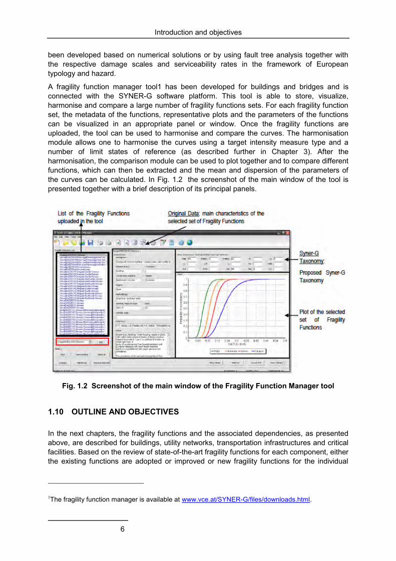
Introduction and objectives
6
been developed based on numerical solutions or by using fault tree analysis together with the respective damage scales and serviceability rates in the framework of European typology and hazard.
A fragility function manager tool1 has been developed for buildings and bridges and is connected with the SYNER-G software platform. This tool is able to store, visualize, harmonise and compare a large number of fragility functions sets. For each fragility function set, the metadata of the functions, representative plots and the parameters of the functions can be visualized in an appropriate panel or window. Once the fragility functions are uploaded, the tool can be used to harmonise and compare the curves. The harmonisation module allows one to harmonise the curves using a target intensity measure type and a number of limit states of reference (as described further in Chapter 3). After the harmonisation, the comparison module can be used to plot together and to compare different functions, which can then be extracted and the mean and dispersion of the parameters of the curves can be calculated. In Fig. 1.2 the screenshot of the main window of the tool is presented together with a brief description of its principal panels.
Fig. 1.2 Screenshot of the main window of the Fragility Function Manager tool
1.10 OUTLINE AND OBJECTIVES
In the next chapters, the fragility functions and the associated dependencies, as presented above, are described for buildings, utility networks, transportation infrastructures and critical facilities. Based on the review of state-of-the-art fragility functions for each component, either the existing functions are adopted or improved or new fragility functions for the individual
1The fragility function manager is available at www.vce.at/SYNER-G/files/downloads.html.

Introduction and objectives
7
components are proposed. For the proposed fragility functions, the following parameters are provided:
o typology classification of each component;
o damage scale definition;
o intensity measure (IM);
o fragility curve parameters, for each damage state and typology.
The objectives of this reference report are summarized as following:
o outline the principles and main issues related to fragility functions;
o classify the available methods for deriving fragility curves;
o review the available fragility functions for each element and system;
o present fragility functions for each element and system of SYNER-G taxonomy.

Methods for deriving fragility functions
9
2 Methods for deriving fragility functions
2.1 INTRODUCTION
The majority of currently available approaches to assess the potential losses for a wide group of exposed elements rely on the availability of relevant fragility curves. In the past decades, the field of seismic risk assessment has witnessed remarkable developments. A detailed review of this subject is presented by Calvi et al. (2006).
Different methods can be employed to develop fragility functions/curves in the field of earthquake engineering. It is commonly agreed to classify them in four generic groups:
o empirical curves, based on observation of actual damage and post-seismic surveys;
o expert opinion-based curves, directly estimated by experts, or based on vulnerability-index models that use expert judgment;
o analytical curves, obtained from the results of static or dynamic analyses of structural models;
o hybrid curves, which can combine any of the above-mentioned techniques, in order to compensate for their respective drawbacks.
The following sections are devoted to the description of these four approaches, along with critical assessment of their qualities and flaws.
2.2 EMPIRICAL METHODS
The study of past earthquakes and the field surveys of actual damages on exposed elements allow compiling extensive statistics on the damage states of various typologies under earthquake laoding. For instance, the study by Spence et al. (1992) has led to fragility curves for 14 classes of buildings, expressed as functions of macroseismic intensity (i.e. Parameterless Scale of Intensity, PSI, also used by Orsini (1999) as shown in Fig. 2.1). These results are based on a survey of 70.000 buildings subjected to 13 different earthquakes. Sabetta et al. (1998) have also developed empirical fragility curves after studying data of 50.000 Italian buildings. The probability of exceeding a damage state is expressed with respect to PGA or spectral response parameters, which are converted from the observed macroseismic intensity. A similar work has been performed by Rota et al. (2006) on Italian buildings. Finally, Rossetto and Elnashai (2003) developed empirical functions for various typologies of RC buildings (moment-resisting frames, infill walls, shear walls) from a database of 340,000 buildings exposed to 19 earthquakes. Empirical relations are also widely used to assess the vulnerability of components that are less prone to analytical developments than buildings, e.g. pipeline segments (ALA, 2001) or tunnels (Corigliano, 2007) and highway embankments (Maruyama, 2010).
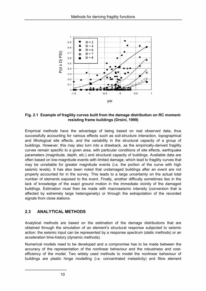
Methods for deriving fragility functions
10
P(d
≥ D
| PSI
)
psi
Fig. 2.1 Example of fragility curves built from the damage distribution on RC moment-resisting frame buildings (Orsini, 1999)
Empirical methods have the advantage of being based on real observed data, thus successfully accounting for various effects such as soil-structure interaction, topographical and lithological site effects, and the variability in the structural capacity of a group of buildings. However, this may also turn into a drawback, as the empirically-derived fragility curves remain specific to a given area, with particular conditions of site effects, earthquake parameters (magnitude, depth, etc.) and structural capacity of buildings. Available data are often based on low-magnitude events with limited damage, which lead to fragility curves that may be unreliable for greater magnitude events (i.e. the portion of the curve with high seismic levels). It has also been noted that undamaged buildings after an event are not properly accounted for in the survey. This leads to a large uncertainty on the actual total number of elements exposed to the event. Finally, another difficulty sometimes lies in the lack of knowledge of the exact ground motion in the immediate vicinity of the damaged buildings. Estimation must then be made with macroseismic intensity (conversion that is affected by extremely large heterogeneity) or through the extrapolation of the recorded signals from close stations.
2.3 ANALYTICAL METHODS
Analytical methods are based on the estimation of the damage distributions that are obtained through the simulation of an element’s structural response subjected to seismic action: the seismic input can be represented by a response spectrum (static methods) or an acceleration time-history (dynamic methods).
Numerical models need to be developed and a compromise has to be made between the accuracy of the representation of the nonlinear behaviour and the robustness and cost-efficiency of the model. Two widely used methods to model the nonlinear behaviour of buildings are plastic hinge modelling (i.e. concentrated inelasticity) and fibre element
Methods for deriving fragility functions
11
modelling (i.e. distributed plasticity). One important choice is representation of the building in 3D or 2D. In the case of structures that are regular in plan, the torsional effects can often be ignored and 2D analyses lead to fairly accurate results.
Regarding the analytical approaches, a distinction can also be made between direct methods that yield fragility curves as functions of ground motion intensity measure types, IMT (e.g. PGA, PGV, Sa(T), etc.) and the “indirect” ones that estimate the damage probability with respect to structural response parameters (e.g. spectral displacement at the inelastic period). The latter approach (expanded upon further in this report in Section 2.2.1), used for instance in the framework of HAZUS (NIBS, 2004) or Risk-UE Level II, (Milutinovic and Trendafilovski, 2003), requires for each seismic scenario computation of the structural response with the capacity curve, and then evaluation of the damage probability using the associated fragility curves.
2.3.1 Dynamic analyses
This approach resides essentially in numerous non-linear dynamic analyses of structural models with a series of acceleration time-histories. Various statistical procedures (maximum likelihood or linear least squares-based) are then used to develop fragility curves that can directly be used in an earthquake scenario.
For instance, Rossetto and Elnashai (2005) have developed fragility curves for 3-story RC buildings with infill walls, by introducing uncertainties in the mechanical properties of concrete, steel and masonry. Kirçiland Polat (2006) have studied bare frame RC buildings with different heights (variability in the number of storeys). The uncertainty on the number of storeys has also been accounted for by Ozmen et al. (2010), who have used 48 3D models of RC buildings. Finally, fragility curves by Erberik (2008) have been developed out of 28 frame models, with or without infills, and with different height configurations.
The dynamic analyses are quite straightforward in the case of individual elements (e.g. specific buildings): however, when analytical fragility curves are developed for a typology or a class of buildings, it is necessary to account for a large variability in the structural response. Therefore uncertainties should be introduced in the
o mechanical properties: these uncertainties enable to represent the variability in the quality of the construction techniques (e.g. wall-floor continuity, amount of reinforcement in RC frames, concrete type, etc.);
o morphological/geometrical properties: in order to represent the whole range of possibilities of buildings included in a given typology, one must model several models that are able to span the whole typology in terms of, for instance, number of storeys, horizontal dimensions, ratio of openings in the walls, irregularities, etc.
Dynamic analyses are often used to derive fragility functions for road elements such as tunnels (Argyroudis, 2010; Salmon et al., 2003) and bridges (Kim and Shinozuka, 2004), because the static procedures, such as pushover approaches, are less adapted to these types of components. For tunnels or embankments, the whole geotechnical system (i.e. accounting for soil-structure interaction) has to be considered and the uncertainties in the soil profiles have to be introduced.
For a given typology, the number of models to analyse can grow dramatically, which leads to a significant number of dynamic analyses. In such studies, sampling techniques, such as
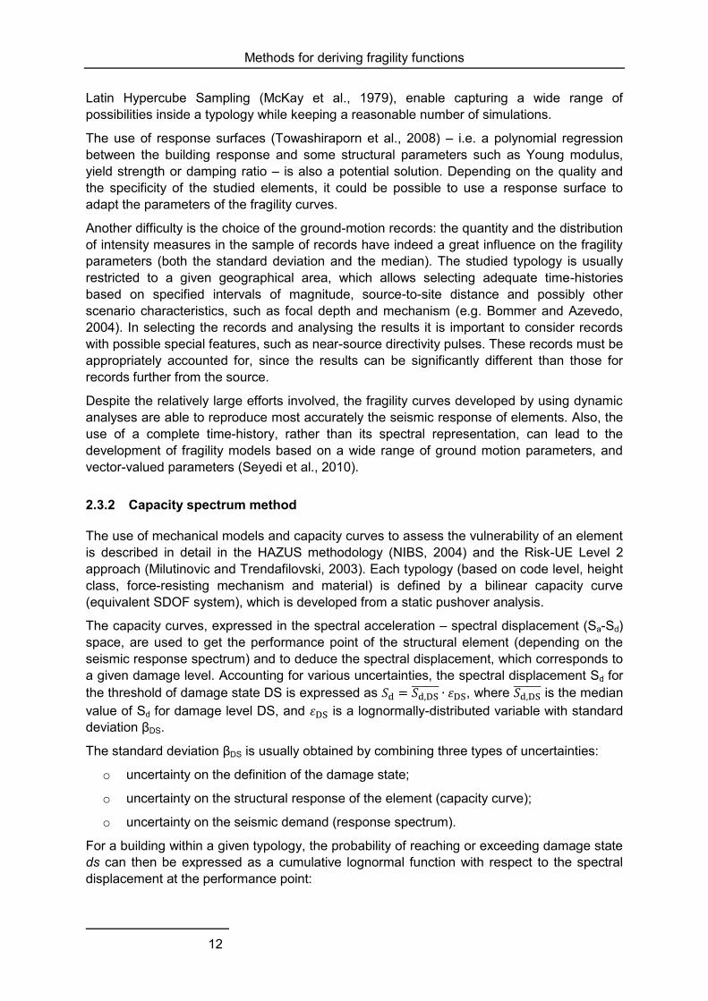
Methods for deriving fragility functions
12
Latin Hypercube Sampling (McKay et al., 1979), enable capturing a wide range of possibilities inside a typology while keeping a reasonable number of simulations.
The use of response surfaces (Towashiraporn et al., 2008) – i.e. a polynomial regression between the building response and some structural parameters such as Young modulus, yield strength or damping ratio – is also a potential solution. Depending on the quality and the specificity of the studied elements, it could be possible to use a response surface to adapt the parameters of the fragility curves.
Another difficulty is the choice of the ground-motion records: the quantity and the distribution of intensity measures in the sample of records have indeed a great influence on the fragility parameters (both the standard deviation and the median). The studied typology is usually restricted to a given geographical area, which allows selecting adequate time-histories based on specified intervals of magnitude, source-to-site distance and possibly other scenario characteristics, such as focal depth and mechanism (e.g. Bommer and Azevedo, 2004). In selecting the records and analysing the results it is important to consider records with possible special features, such as near-source directivity pulses. These records must be appropriately accounted for, since the results can be significantly different than those for records further from the source.
Despite the relatively large efforts involved, the fragility curves developed by using dynamic analyses are able to reproduce most accurately the seismic response of elements. Also, the use of a complete time-history, rather than its spectral representation, can lead to the development of fragility models based on a wide range of ground motion parameters, and vector-valued parameters (Seyedi et al., 2010).
2.3.2 Capacity spectrum method
The use of mechanical models and capacity curves to assess the vulnerability of an element is described in detail in the HAZUS methodology (NIBS, 2004) and the Risk-UE Level 2 approach (Milutinovic and Trendafilovski, 2003). Each typology (based on code level, height class, force-resisting mechanism and material) is defined by a bilinear capacity curve (equivalent SDOF system), which is developed from a static pushover analysis.
The capacity curves, expressed in the spectral acceleration – spectral displacement (Sa-Sd) space, are used to get the performance point of the structural element (depending on the seismic response spectrum) and to deduce the spectral displacement, which corresponds to a given damage level. Accounting for various uncertainties, the spectral displacement Sd for the threshold of damage state DS is expressed as , where is the median value of Sd for damage level DS, and is a lognormally-distributed variable with standard deviation βDS.
The standard deviation βDS is usually obtained by combining three types of uncertainties:
o uncertainty on the definition of the damage state;
o uncertainty on the structural response of the element (capacity curve);
o uncertainty on the seismic demand (response spectrum).
For a building within a given typology, the probability of reaching or exceeding damage state ds can then be expressed as a cumulative lognormal function with respect to the spectral displacement at the performance point:
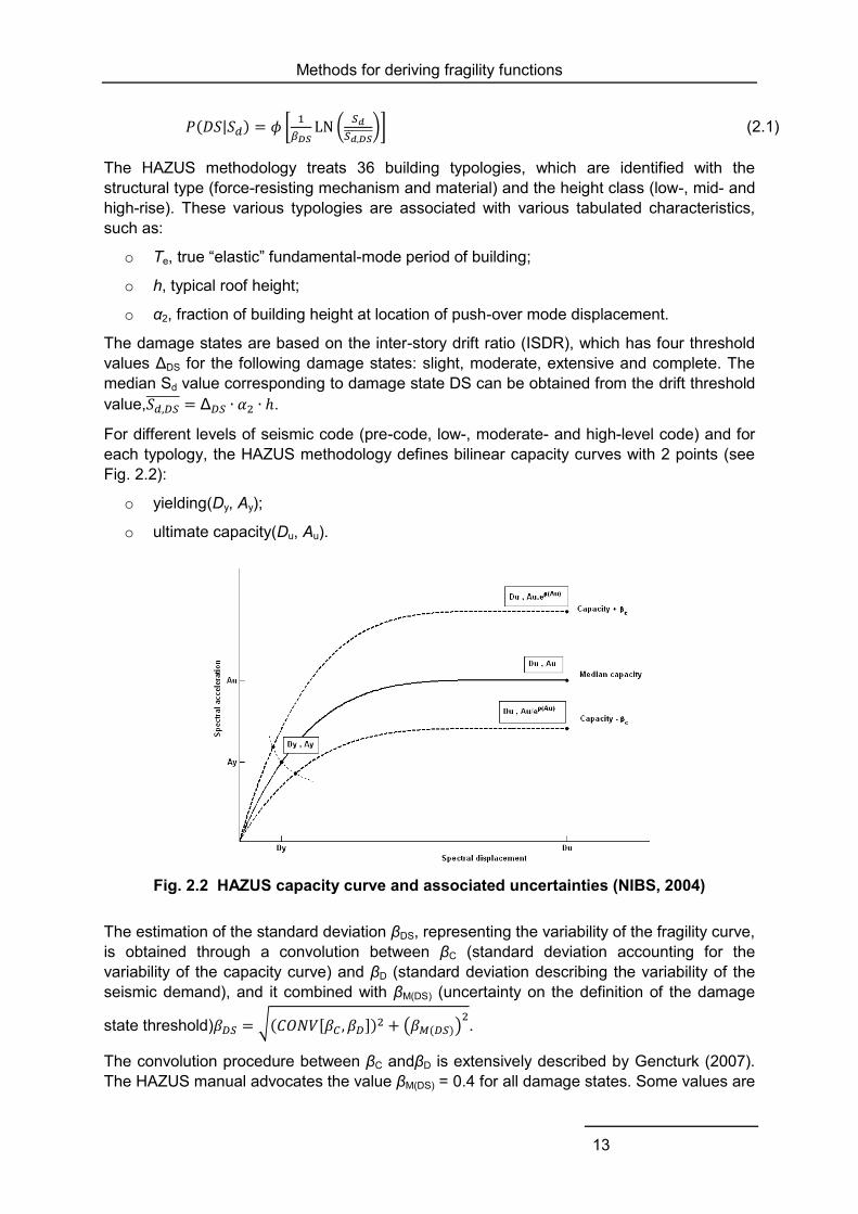
Methods for deriving fragility functions
13
( | ) [
(
)] (2.1)
The HAZUS methodology treats 36 building typologies, which are identified with the structural type (force-resisting mechanism and material) and the height class (low-, mid- and high-rise). These various typologies are associated with various tabulated characteristics, such as:
o Te, true “elastic” fundamental-mode period of building;
o h, typical roof height;
o α2, fraction of building height at location of push-over mode displacement.
The damage states are based on the inter-story drift ratio (ISDR), which has four threshold values ΔDS for the following damage states: slight, moderate, extensive and complete. The median Sd value corresponding to damage state DS can be obtained from the drift threshold value, Δ .
For different levels of seismic code (pre-code, low-, moderate- and high-level code) and for each typology, the HAZUS methodology defines bilinear capacity curves with 2 points (see Fig. 2.2):
o yielding(Dy, Ay);
o ultimate capacity(Du, Au).
Fig. 2.2 HAZUS capacity curve and associated uncertainties (NIBS, 2004)
The estimation of the standard deviation βDS, representing the variability of the fragility curve, is obtained through a convolution between βC (standard deviation accounting for the variability of the capacity curve) and βD (standard deviation describing the variability of the seismic demand), and it combined with βM(DS) (uncertainty on the definition of the damage
state threshold) √( [ ]) ( ( )) .
The convolution procedure between βC andβD is extensively described by Gencturk (2007). The HAZUS manual advocates the value βM(DS) = 0.4 for all damage states. Some values are

Methods for deriving fragility functions
14
also recommended for the variability on the capacity curve: βC(Au) = 0.25 for code-compliant elements and βC(Au) = 0.3 for pre-code constructions.
In the Risk-UE project, the Level 2 approach relies on the same main steps as the HAZUS procedure:
o typological classification of the elements;
o development of capacity curves;
o determination of the performance point based on the seismic level;
o assessment of the probabilities to reach or exceed the different damage states.
The two approaches obviously diverge in terms of input data and the Risk-UE method proposes typologies that are adapted to the European context, as well as specific capacity curves. The damage state definitions rely on ISDR values that are identified based on the capacity curve: the drift values are then structure-specific, as opposed to HAZUS, which recommends fixed values for each typology. Table 2.1, taken from the Risk-UE approach, gives threshold values for each damage state, as a function of yielding and ultimate capacity points.
Table 2.1 Damage state definitions (Risk-UE)
Damage state Drift limit Spectral displacement limit
DS1 No damage Δ< 0.7Δy D< 0.7Dy DS2 Slight 0.7Δy<Δ< 0.7Δy + 0.05Δuy 0.7Dy<D<Dy DS3 Moderate 0.7Δy + 0.05Δuy<Δ< 0.7Δy + 0.2Δuy Dy<D<Dy + Duy DS4 Extensive 0.7Δy + 0.2Δuy<Δ< 0.7Δy + 0.5Δuy Dy + Duy<D<Du DS5 Very heavy 0.7Δy + 0.5Δuy<Δ< 0.7Δy + Δuy Du<D
With: Δuy = 0.9Δu - 0.7Δy and Duy = 0.25(Du – Dy)
It has to be noted that nonlinear static analyses can also be used to generate “direct” fragility curves that do not necessarily rely on the structural response parameter. The response spectrum can be used to associate each estimated performance point with the equivalent intensity measure (e.g. PGA) of the seismic records that are used (NIBS, 2004). Therefore, the fragility curves can be used as stand-alone function to directly estimate the damage probability, without going through the capacity curve.
2.4 EXPERT JUDGEMENT
2.4.1 Curves based on expert opinion
This procedure, which may be considered out-dated nowadays, entirely relies on the judgment of some experts who are asked to provide an estimate of the mean loss or probability of damage of a given element for different levels of seismic loading. Some of the fragility curves proposed in HAZUS (e.g. roads and tunnels) are developed using this method. The procedure is described in the ATC13 (ATC, 1985) documents.
Methods for deriving fragility functions
15
This technique has the advantage of not being affected by the lack of extensive damage data (empirical approaches) or the reliability or the structural model used in analytical developments. However, the results rely solely on the individual experience of the experts consulted. The potential bias in the curves can be reduced by extending the number of experts and by assigning some weight to their estimations, based on their expertise level (Porter et al., 2007).
2.4.2 Macroseismic models
A widely used approach is also to estimate vulnerability indexes based on a visual diagnostic (expert opinion-based) of a group of buildings. Several characteristics can be observed: force-resisting mechanism and material, floor types, building height, soft stories, quality of construction, irregularities, non-structural elements, age of building, etc.
For instance, in the Risk-UE project, the Level 1 approach (Milutinovic and Trendafilovski, 2003) defines a vulnerability index Vi, between 0 and 1, based on the observed characteristics of the element. The index is expressed as Vi = Vi
* + Vm +VR. The index Vi* is
defined as the most probable index for the studied typology. For each Risk-UE typology, the probable values, as well as the lower and upper boundaries, are presented in

Methods for deriving fragility functions
16
Table 2.2. The index Vm is a behaviour modification factor, shown in Table 2.3, based on the specific characteristics of the structure. Positive or negative factors can then be summed to alter the global vulnerability.
The index VR is a regional vulnerability factor. It is used to account for the global construction quality of a given area and it is based on expert judgment. Finally, an uncertainty level can be added to Vi by considering an interval ΔVf, which is defined by the type of data used in the study (for instance: 0.04 if a specific seismic vulnerability database is used, and 0.08 if data are more generic).
An empirical relation can then express the mean damage grade as a function of Vi and macroseismic intensity, [ (
)], where µD stands for the mean
damage grade (between 0 and 5) and I is the macroseismic intensity (Fig. 2.3).
From the mean damage grade, a damage distribution (beta law) can be expressed with the following, which probability density function.
( ) ( )
( ) ( ) ( ) ( )
( ) (2.2)
with α ≤ x<b.
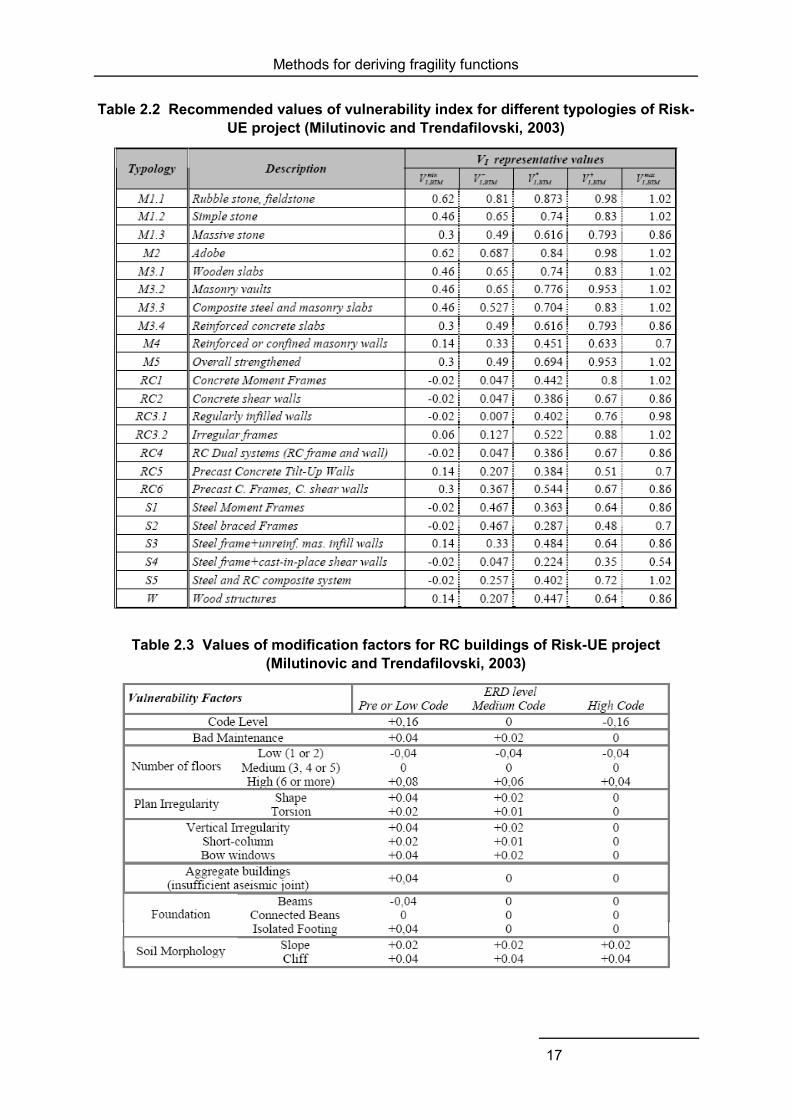
Methods for deriving fragility functions
17
Table 2.2 Recommended values of vulnerability index for different typologies of Risk-UE project (Milutinovic and Trendafilovski, 2003)
Table 2.3 Values of modification factors for RC buildings of Risk-UE project (Milutinovic and Trendafilovski, 2003)

Methods for deriving fragility functions
18
Based on the EMS-98 damage scale, six damage states are possible (between 0 and 5), and it is recommended to set α = 0 and b = 6 (Lagomarsino and Giovinazzi, 2006). The parameters of the beta law are defined as q = t (0.007μD
3 – 0.052μD2 + 0.287μD). The
parameter t, which controls the slope of the distribution, can for instance be set to t = 8 in order to be close to a binomial distribution (Sedan et al., 2008). The cumulative density of the beta law can finally be used to compute the probability that a building with vulnerability index Vi reaches or exceeds a given damage state: ( ) ∫ ( )
.
Fig. 2.3 Evolution of µD with respect to intensity, I, for different typologies of RISK-UE
project (Milutinovic and Trendafilovski, 2003)
2.5 HYBRID METHODS
Hybrid fragility curves are the result of a combination of methods, using for instance both analytical and observational data, or completed by expert judgment. The main advantage is that they compensate for the lack of observational data for the deficiencies of structural models and for the subjectivity in expert opinion data. For instance, analytical fragility curves can be modified and improved by integrating post-seismic observations that are made available after the initial development. This kind of approach enables one to calibrate the analytical results (which are usually based on more or less justified assumptions) or to fill-in some blanks due to scarce data at high seismic levels (Calvi et al., 2006). The addition of empirical data to analytical curves can be done through Bayesian updating, resulting in new estimations of the median and standard deviation of the initial lognormal distribution (Singhal and Kiremidjian, 1998). Finally, another example is the work by Kappos et al. (2006a), where fragility curves for RC and unreinforced masonry buildings are derived using both statistical data from earthquake-damaged Greek buildings and results from nonlinear static or dynamic analyses.

Fragility functions for buildings
19
3 Fragility functions for buildings
The identification of the seismic fragility functions for common buildings types is a fundamental component of a seismic risk loss assessment model and, for this reason, many research studies have addressed this topic in the recent past.
In the context of the SYNER-G Project the main typologies of buildings in Europe have been identified and, focusing on reinforced concrete and masonry buildings, the existing fragility functions have been reviewed with the objective of homogenizing the existing model building types (through a new taxonomy, called the SYNER-G taxonomy), and comparing these functions amongst themselves. The main output is a set of fragility functions (with associated uncertainties) for the main reinforced concrete and masonry typologies present in Europe.
In the following paragraphs, the methodologies, intensity measure types and limit states that have been identified in the reviewed fragility studies for European buildings, as well as the taxonomies used to describe different building classes, and the procedures to harmonize and compare fragility curves for a given building typology are presented and described.
For further details, the reader is referred to SYNER-G’s Deliverables 3.1 and 3.2.
3.1 REVIEW OF FRAGILITY FUNCTIONS FOR EUROPEAN BUILDINGS
In the European continent, most of the buildings are constructed with masonry or reinforced concrete, and for this reason, the majority of the existing fragility functions treat these two types of structures. Fragility functions describe the probability of exceeding different limit states (such as damage levels) given a level of ground shaking. A “fragility function set”, as referred to herein, represents a group of functions for a given building typology for a number of different limit states of damage.
3.1.1 Definition of limit states
As mentioned in Section 1.1, a fragility function set is described according to different limit states that define the threshold between different damage conditions. For instance, if the performance of a building is described by two limit states (Limit State 1 and Limit State 2), there will be three damage states (Damage State 1, Damage State 2 and Damage State 3), as shown in Fig. 3.1.
Methods for deriving fragility curves generally model the damage on a discrete damage scale. In empirical procedures, the scale is used in reconnaissance efforts to produce post-earthquake damage statistics, whereas in analytical procedures the scale is related to limit state mechanical properties of the buildings, such as displacement capacity or inter-storey drift capacity.

Fragility functions for buildings
20
Fig. 3.1 Limit States and Damage States
The number of Damage States (and consequently the number of Limit States) depends on the damage scale used. Some of the most frequently used damage scales are: HCR (Rossetto and Elnashai, 2003), HAZUS99 (FEMA, 1999), Vision2000 (SEAOC, 1995), EMS98 (Grunthal, 1998), and ATC-13 (ATC, 1985). A summary and qualitative comparison of some of the damage scales used in the selected fragility functions with the Homogenised Reinforced Concrete (HRC) damage scale (Rossetto and Elnashai, 2003) is presented in the following table.
Table 3.1 Comparison of existing damage scales with HRC damage scale [adapted from Rossetto and Elnashai, 2003]
HRC HAZUS99 Vision 2000 EMS98 ATC-13
None No damage
Slight
Slight damage
Fully operational Grade 1
Slight
Light Light
Operational Grade 2
Moderate Moderate Moderate
damage Grade 3 Life Safe
Heavy Extensive
Extensive damage
Near Collapse
Grade 4 Major Partial
Collapse Collapse
Collapse Collapse
Lateral Load
Damage State 1
Limit State 1
Displacement
Damage State 2
Damage State 3
Limit State 2

Fragility functions for buildings
21
Depending on the methodology used to compute the fragility functions and depending on the choices by the authors, different scales with different limit states/damage states can be adopted. It should be noted that there are some studies that do not refer to any of the damage scales reported above, but they follow specific damage scales developed by the authors.
3.1.2 Key elements in definition of fragility function
A large number of fragility functions have been collected in the context of the SYNER-G project and they have been stored into a dynamic tool, the SYNER-G Fragility Function Manager, which is briefly described in Chapter 1. For each fragility study that has been considered, a review form has been filled in with a brief summary of the functions. A complete list of the analysed studies can be found in the Appendices of SYNER-G Deliverables 3.1 and 3.2. The form contains the available information about the key elements that identify a fragility function set. The fields inserted in the form are given the following:
o Reference: reference papers, publications, documents, deliverables;
o Region of applicability: the reference place for which the structures and buildings have been analysed and for which the fragility functions have been developed;
o Element at risk: list of the elements that the fragility functions can be used to model (e.g., buildings, bridges, lifelines, infrastructures, etc.);
o Typology of the element at risk: based on the original description provided in the references (e.g. RC – low rise – high code; masonry – simple stone; steel, etc.);
o SYNER-G Taxonomy: the description of the element at risk using the taxonomy proposed within the SYNER-G project (see SYNER-G Reference Report 2);
o Sample Data: description of the data (e.g. structures, accelerograms, etc.) that are considered in the analyses to estimate the fragility functions;
o Methodology: empirical, analytical, hybrid etc. (as described in Chapter 2);
o Intensity Measure Type (IMT): the reference parameter against which the probability of exceedance of a given limit state is plotted (e.g. macroseismic Intensity, PGV, PGA, spectral acceleration at fundamental period, etc.);
o Fragility Function Parameters: description of the parameters used to define the fragility functions (e.g. mean and standard deviation of a particular distribution);
o Figures: plot(s) of the fragility function sets created by the Fragility Function Manager tool;
o Uncertainty: description of the sources of uncertainty that have been taken into account for the estimation of the fragility curves (i.e., the variability in the properties of the materials, the variability of the geometry of the structures, record-to-record variability etc.);
o Comments: any additional notes and comments.
An example of a compiled review form is shown in Fig. 3.2. The other review forms can be found in the Appendix A of Deliverables 3.1 and 3.2 of SYNER-G.

Fragility functions for buildings
22
KapposEtAl2006
Reference A. J. Kappos, G. Panagopoulos, C.Panagiotopoulos, G. Penelis, “A hybrid method for the vulnerability
assessment of R/C and URM buildings” Bulletin of Earthquake Engineering, 4, 391-413, 2006.
Region of
applicability
Greece
Element at risk Buildings
Typology of
element at risk
considered
Reinforced Concrete and Unreinforced Masonry structures.
Reinforced Concrete Legend:
Type Structural System Height (number
of storeys)
Seismic Design
Level
RC1 Concrete moment frame
(L)ow-rise (1-3)
(M)id-rise (4-7)
(H)igh-rise (8+)
(N)o/pre code
(L)ow code
(M)edium code
(H)igh code
RC3.1 RC regularly infilled frame
RC3.2 RC irregularly infilled frame (pilotis)
RC4.1 RC dual systems – bare frames
RC4.2 RC dual systems - regularly infilled dual system
RC4.3 RC dual systems - irregularly infilled dual
system (pilotis)
Syner-G
Taxonomy
MRF/C/RC/R/R/B-X/ND/X-X/X-X/HR-X/LC
MRF/C/RC/R/R/RI-FB/ND/X-X/X-X/HR-X/LC
MRF/C/RC/R/R/IRI-FB-P/ND/X-X/X-X/HR-X/LC
MRF-W/C/RC/R/R/B-X/ND/X-X/X-X/HR-X/LC
MRF-W/C/RC/R/R/RI-FB/ND/X-X/X-X/HR-X/LC
MRF-W/C/RC/R/R/IRI-FB-P/ND/X-X/X-X/HR-X/LC
MRF/C/RF/R/R/RI-FB/ND/X-X/X-X/MR-X/LC
MRF/C/RC/R/R/RI-FB/D/X-X/X-X/MR-X/HC
MRF/C/RC/R/R/RI-FB/ND/X-X/X-X/MR-X/LC
MRF-W/C/RC/R/R/RI-FB/D/X-X/X-X/MR-X/HC
MRF/C/RC/R/R/B-X/D/X-X/X-X/HR-X/HC
MRF/C/RC/R/R/RI-FB/D/X-X/X-X/HR-X/HC
MRF/C/RC/R/R/IRI-FB-P/D/X-X/X-X/HR-X/HC
MRF-W/C/RC/R/R/B-X/D/X-X/X-X/HR-X/HC
MRF-W/C/RC/R/R/RI-FB/D/X-X/X-X/HR-X/HC
MRF-W/C/RC/P/P/IRI-FB-P/D/X-X/X-X/HR-X/HC
MRF/C/RC/R/R/RI-FB/ND/X-X/X-X/MR-X/LC
MRF/C/RC/R/R/RI-FB/D/X-X/X-X/MR-X/HC
BW/M/URM-FB/X/X/X-X/X/X-X/X-X/LR-2/NC
BW/M/URM-S/X/X/X-X/X/X-X/X-X/LR-2/NC
Sample data Buildings: earthquake-damaged Greek buildings + a large number of building types are modelled and
analyzed
Seismic Hazard: real earthquakes (1978 Thessaloniki earthquake) and 16 accelerograms.

Fragility functions for buildings
23
Methodology Hybrid approach combines statistical data with appropriately processed results from nonlinear dynamic or
static analyses
Damage States Six damage states are considered:
DS0 – No damage
DS1 – Slight
DS2 – Moderate
DS3 – Substantial to Heavy
DS4 – Very Heavy
DS5 – Complete
Intensity
Measure Type
PGA [g] and Sd(Ty) [cm]
Fragility Function
Parameters
Lognormal distribution
IMT = PGA [g]
DS1 DS2 DS3 DS4 DS5
Mean StDev Mean StDev Mean StDev Mean StDev Mean StDev
RC1HL 0.007 0.005 0.074 0.052 0.181 0.127 0.336 0.234 0.664 0.463
RC3.1HL 0.016 0.011 0.118 0.082 0.256 0.178 0.361 0.251 0.668 0.465
RC3.2HL 0.054 0.037 0.123 0.086 0.255 0.177 0.430 0.300 0.820 0.571
RC4.1HL 0.003 0.002 0.024 0.019 0.270 0.214 1.028 0.818 3.943 3.135
RC4.2HL 0.050 0.040 0.144 0.115 0.337 0.268 1.108 0.881 4.910 3.904
RC4.3HL 0.065 0.052 0.148 0.118 0.368 0.292 1.258 1.001 3.873 3.079
RC3.1ML 0.020 0.013 0.069 0.047 0.252 0.204 0.279 0.198 0.316 0.212
RC3.1MH 0.620 0.041 0.137 0.085 0.352 0.267 0.702 0.469 1.547 1.098
RC4.2ML 0.024 0.017 0.174 0.152 0.416 0.315 0.703 0.569 0.906 0.691
RC4.2MH 0.098 0.081 0.236 0.183 0.649 0.513 1.234 0.898 2.471 1.841
IMT = Sd(Ty) [cm]
DS1 DS2 DS3 DS4 DS5
Mean StDev Mean StDev Mean StDev Mean StDev Mean StDev
RC1HH 0.481 0.321 3.847 2.568 20.198 13.481 56.387 37.636 91.855 61.308
RC3.1HH 0.601 0.401 3.246 2.167 12.023 8.025 36.670 24.475 72.979 48.710
RC3.2HH 2.284 1.525 5.651 3.772 15.028 10.031 24.166 16.130 42.801 28.568
RC4.1HH 1.260 0.966 5.544 4.251 36.669 28.116 76.363 58.550 131.18 100.578
RC4.2HH 1.260 0.966 4.788 3.671 32.511 24.927 64.644 49.564 129.54 99.322
RC4.3HH 1.512 1.159 5.292 4.058 22.430 17.198 65.652 50.337 122.10 93.622
RC3.1ML 0.213 0.157 0.743 0.578 2.473 1.765 2.785 1.925 3.285 2.377
RC3.1MH 0.460 0.270 1.200 0.693 2.310 1.500 5.090 3.790 10.740 7.500
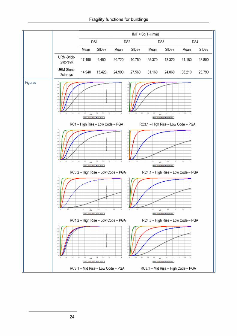
Fragility functions for buildings
24
IMT = Sd(Ty) [mm]
DS1 DS2 DS3 DS4
Mean StDev Mean StDev Mean StDev Mean StDev
URM-Brick-
2storeys 17.190 9.450 20.720 10.750 25.370 13.320 41.180 28.800
URM-Stone-
2storeys 14.940 13.420 24.990 27.560 31.160 24.060 36.210 23.790
Figures
RC1 – High Rise – Low Code – PGA RC3.1 – High Rise – Low Code – PGA
RC3.2 – High Rise – Low Code – PGA RC4.1 – High Rise – Low Code – PGA
RC4.2 – High Rise – Low Code – PGA RC4.3 – High Rise – Low Code – PGA
RC3.1 – Mid Rise – Low Code – PGA RC3.1 – Mid Rise – High Code – PGA
DS1 DS2 DS3 DS4 DS5
PGA21.81.61.41.210.80.60.40.20
Prob
abilit
y of
exc
eeda
nce
1
0.9
0.8
0.7
0.6
0.5
0.4
0.3
0.2
0.1
0
DS1 DS2 DS3 DS4 DS5
PGA21.81.61.41.210.80.60.40.20
Prob
abilit
y of
exc
eeda
nce
1
0.9
0.8
0.7
0.6
0.5
0.4
0.3
0.2
0.1
0
DS1 DS2 DS3 DS4 DS5
PGA21.81.61.41.210.80.60.40.20
Prob
abilit
y of
exc
eeda
nce
1
0.9
0.8
0.7
0.6
0.5
0.4
0.3
0.2
0.1
0
DS1 DS2 DS3 DS4 DS5
PGA43.532.521.510.50
Prob
abilit
y of
exc
eeda
nce
1
0.9
0.8
0.7
0.6
0.5
0.4
0.3
0.2
0.1
0
DS1 DS2 DS3 DS4 DS5
PGA43.532.521.510.50
Prob
abilit
y of
exc
eeda
nce
1
0.9
0.8
0.7
0.6
0.5
0.4
0.3
0.2
0.1
0
DS1 DS2 DS3 DS4 DS5
PGA43.532.521.510.50
Prob
abilit
y of
exc
eeda
nce
1
0.9
0.8
0.7
0.6
0.5
0.4
0.3
0.2
0.1
0
DS1 DS2 DS3 DS4 DS5
PGA21.81.61.41.210.80.60.40.20
Prob
abilit
y of
exc
eeda
nce
1
0.9
0.8
0.7
0.6
0.5
0.4
0.3
0.2
0.1
0
DS1 DS2 DS3 DS4 DS5
PGA21.81.61.41.210.80.60.40.20
Prob
abilit
y of
exc
eeda
nce
1
0.9
0.8
0.7
0.6
0.5
0.4
0.3
0.2
0.1
0
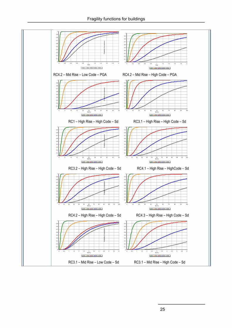
Fragility functions for buildings
25
RC4.2 – Mid Rise – Low Code – PGA RC4.2 – Mid Rise – High Code – PGA
RC1 – High Rise – High Code – Sd RC3.1 – High Rise – High Code – Sd
RC3.2 – High Rise – High Code – Sd RC4.1 – High Rise – HighCode – Sd
RC4.2 – High Rise – High Code – Sd RC4.3 – High Rise – High Code – Sd
RC3.1 – Mid Rise – Low Code – Sd RC3.1 – Mid Rise – High Code – Sd
DS1 DS2 DS3 DS4 DS5
PGA21.81.61.41.210.80.60.40.20
Prob
abilit
y of
exc
eeda
nce
1
0.9
0.8
0.7
0.6
0.5
0.4
0.3
0.2
0.1
0
DS1 DS2 DS3 DS4 DS5
PGA21.81.61.41.210.80.60.40.20
Prob
abilit
y of
exc
eeda
nce
1
0.9
0.8
0.7
0.6
0.5
0.4
0.3
0.2
0.1
0
DS1 DS2 DS3 DS4 DS5
Sd(Ty)50454035302520151050
Prob
abilit
y of
exc
eeda
nce
1
0.9
0.8
0.7
0.6
0.5
0.4
0.3
0.2
0.1
0
DS1 DS2 DS3 DS4 DS5
Sd(Ty)1009080706050403020100
Prob
abilit
y of
exc
eeda
nce
1
0.9
0.8
0.7
0.6
0.5
0.4
0.3
0.2
0.1
0
DS1 DS2 DS3 DS4 DS5
Sd(Ty)50454035302520151050
Prob
abilit
y of
exc
eeda
nce
1
0.9
0.8
0.7
0.6
0.5
0.4
0.3
0.2
0.1
0
DS1 DS2 DS3 DS4 DS5
Sd(Ty)1201101009080706050403020100
Prob
abilit
y of
exc
eeda
nce
1
0.9
0.8
0.7
0.6
0.5
0.4
0.3
0.2
0.1
0
DS1 DS2 DS3 DS4 DS5
Sd(Ty)1201101009080706050403020100
Prob
abilit
y of
exc
eeda
nce
1
0.9
0.8
0.7
0.6
0.5
0.4
0.3
0.2
0.1
0
DS1 DS2 DS3 DS4 DS5
Sd(Ty)1009080706050403020100
Prob
abilit
y of
exc
eeda
nce
1
0.9
0.8
0.7
0.6
0.5
0.4
0.3
0.2
0.1
0
DS1 DS2 DS3 DS4 DS5
Sd(Ty)65.554.543.532.521.510.50
Prob
abilit
y of
exc
eeda
nce
1
0.9
0.8
0.7
0.6
0.5
0.4
0.3
0.2
0.1
0
DS1 DS2 DS3 DS4 DS5
Sd(Ty)65.554.543.532.521.510.50
Prob
abilit
y of
exc
eeda
nce
1
0.9
0.8
0.7
0.6
0.5
0.4
0.3
0.2
0.1
0
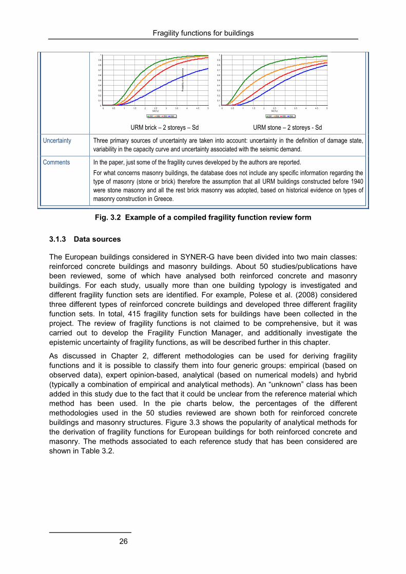
Fragility functions for buildings
26
URM brick – 2 storeys – Sd URM stone – 2 storeys - Sd
Uncertainty Three primary sources of uncertainty are taken into account: uncertainty in the definition of damage state,
variability in the capacity curve and uncertainty associated with the seismic demand.
Comments In the paper, just some of the fragility curves developed by the authors are reported.
For what concerns masonry buildings, the database does not include any specific information regarding the
type of masonry (stone or brick) therefore the assumption that all URM buildings constructed before 1940
were stone masonry and all the rest brick masonry was adopted, based on historical evidence on types of
masonry construction in Greece.
Fig. 3.2 Example of a compiled fragility function review form
3.1.3 Data sources
The European buildings considered in SYNER-G have been divided into two main classes: reinforced concrete buildings and masonry buildings. About 50 studies/publications have been reviewed, some of which have analysed both reinforced concrete and masonry buildings. For each study, usually more than one building typology is investigated and different fragility function sets are identified. For example, Polese et al. (2008) considered three different types of reinforced concrete buildings and developed three different fragility function sets. In total, 415 fragility function sets for buildings have been collected in the project. The review of fragility functions is not claimed to be comprehensive, but it was carried out to develop the Fragility Function Manager, and additionally investigate the epistemic uncertainty of fragility functions, as will be described further in this chapter.
As discussed in Chapter 2, different methodologies can be used for deriving fragility functions and it is possible to classify them into four generic groups: empirical (based on observed data), expert opinion-based, analytical (based on numerical models) and hybrid (typically a combination of empirical and analytical methods). An “unknown” class has been added in this study due to the fact that it could be unclear from the reference material which method has been used. In the pie charts below, the percentages of the different methodologies used in the 50 studies reviewed are shown both for reinforced concrete buildings and masonry structures. Figure 3.3 shows the popularity of analytical methods for the derivation of fragility functions for European buildings for both reinforced concrete and masonry. The methods associated to each reference study that has been considered are shown in Table 3.2.
DS1 DS2 DS3 DS4
Sd(Ty)54.543.532.521.510.50
Prob
abilit
y of
exc
eeda
nce
1
0.9
0.8
0.7
0.6
0.5
0.4
0.3
0.2
0.1
0
DS1 DS2 DS3 DS4
Sd(Ty)54.543.532.521.510.50
Prob
abilit
y of
exc
eeda
nce
1
0.9
0.8
0.7
0.6
0.5
0.4
0.3
0.2
0.1
0
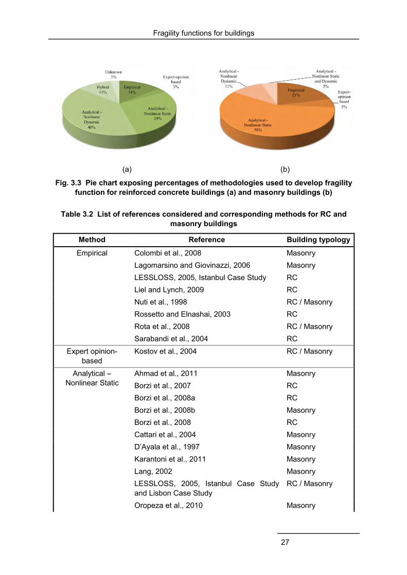
Fragility functions for buildings
27
(a)
(b)
Fig. 3.3 Pie chart exposing percentages of methodologies used to develop fragility function for reinforced concrete buildings (a) and masonry buildings (b)
Table 3.2 List of references considered and corresponding methods for RC and masonry buildings
Method Reference Building typology
Empirical Colombi et al., 2008 Masonry Lagomarsino and Giovinazzi, 2006 Masonry LESSLOSS, 2005, Istanbul Case Study RC Liel and Lynch, 2009 RC Nuti et al., 1998 RC / Masonry Rossetto and Elnashai, 2003 RC Rota et al., 2008 RC / Masonry Sarabandi et al., 2004 RC
Expert opinion-based
Kostov et al., 2004 RC / Masonry
Analytical – Nonlinear Static
Ahmad et al., 2011 Masonry Borzi et al., 2007 RC Borzi et al., 2008a RC Borzi et al., 2008b Masonry Borzi et al., 2008 RC Cattari et al., 2004 Masonry D’Ayala et al., 1997 Masonry Karantoni et al., 2011 Masonry Lang, 2002 Masonry LESSLOSS, 2005, Istanbul Case Study and Lisbon Case Study
RC / Masonry
Oropeza et al., 2010 Masonry

Fragility functions for buildings
28
Method Reference Building typology
Pagnini et al., 2008 Masonry Polese et al., 2008 RC RISK-UE, 2003, CIMNE approach RC / Masonry RISK-UE, 2003, UTCB approach RC Tsionis et al., 2011 RC Vacareanu et al., 2004 RC Varga et al., 2010 RC
Analytical – Nonlinear Dynamic
Ahmad et al., 2011 RC Akkar et al., 2005 RC Dumova-Jovanoska, 2000 RC Erberik and Elnashai, 2004 RC Erberik, 2008 RC Hancilar et al., 2006 RC Hancilar et al., 2007 RC Jeong and Elnashai, 2007 RC Kirçil and Polat, 2006 RC Kwon and Elnashai, 2007 RC Ozmen et al., 2010 RC RISK-UE, 2003, IZIIS approach RC RISK-UE, 2003, UNIGE approach Masonry Rossetto and Elnashai, 2005 RC
Rota et al., 2010 Masonry
Analytical – Nonlinear Static and
Dynamic
Erberik, 2008 Masonry
Hybrid Kappos et al., 2006a RC RISK-UE, 2003 (AUTH, IZIIS and UTCB approach)
RC
Unknown Tahiri and Milutinovic, 2010 RC
Another key element, which is significant in the development of the fragility curves, is the Intensity Measure Type (IMT) that represents the reference ground motion parameter against which the probability of exceedance of a given limit state is plotted. The vulnerable conditions of a structure are defined for a certain level of ground shaking. An intensity measure describes the severity of earthquake shaking.
In the reviewed papers, different IMTs have been used to define the level of ground shaking. It is possible to group these IMTs into two main classes: observational intensity measure types and instrumental intensity measure types.
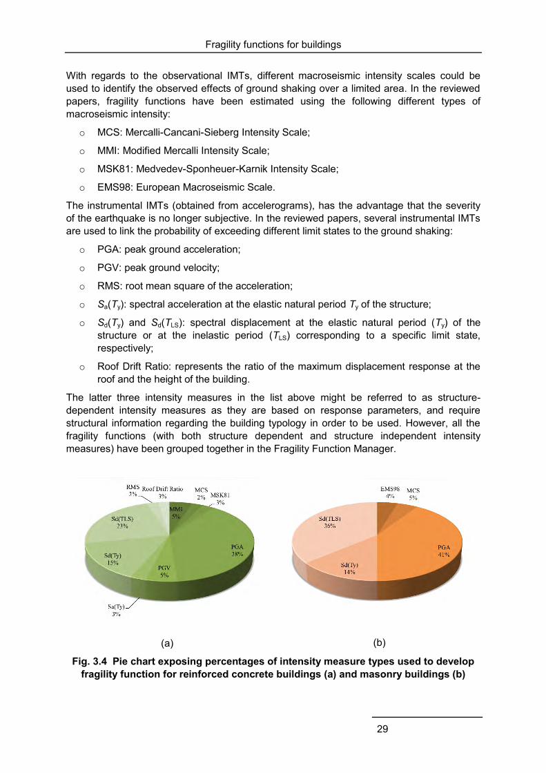
Fragility functions for buildings
29
With regards to the observational IMTs, different macroseismic intensity scales could be used to identify the observed effects of ground shaking over a limited area. In the reviewed papers, fragility functions have been estimated using the following different types of macroseismic intensity:
o MCS: Mercalli-Cancani-Sieberg Intensity Scale;
o MMI: Modified Mercalli Intensity Scale;
o MSK81: Medvedev-Sponheuer-Karnik Intensity Scale;
o EMS98: European Macroseismic Scale.
The instrumental IMTs (obtained from accelerograms), has the advantage that the severity of the earthquake is no longer subjective. In the reviewed papers, several instrumental IMTs are used to link the probability of exceeding different limit states to the ground shaking:
o PGA: peak ground acceleration;
o PGV: peak ground velocity;
o RMS: root mean square of the acceleration;
o Sa(Ty): spectral acceleration at the elastic natural period Ty of the structure;
o Sd(Ty) and Sd(TLS): spectral displacement at the elastic natural period (Ty) of the structure or at the inelastic period (TLS) corresponding to a specific limit state, respectively;
o Roof Drift Ratio: represents the ratio of the maximum displacement response at the roof and the height of the building.
The latter three intensity measures in the list above might be referred to as structure-dependent intensity measures as they are based on response parameters, and require structural information regarding the building typology in order to be used. However, all the fragility functions (with both structure dependent and structure independent intensity measures) have been grouped together in the Fragility Function Manager.
(a)
(b)
Fig. 3.4 Pie chart exposing percentages of intensity measure types used to develop fragility function for reinforced concrete buildings (a) and masonry buildings (b)

Fragility functions for buildings
30
In Fig. 3.4, the percentages concerning the different IMTs used in the studies are shown both for reinforced concrete buildings and masonry structures. As it can be noted, the peak ground acceleration has been the most commonly used intensity measure type to develop fragility functions in Europe.
3.2 NEW FRAGILITY CURVES FOR RC AND MASONRY BUILDINGS
3.2.1 Fragility curves for RC frame and dual buildings designed according to Eurocode 2 and 8
Within SYNER-G, new fragility curves were produced for a portfolio of prototype plan- and height-wise regular RC frame and wall-frame buildings designed and detailed to Eurocode 2 (EC2) and Eurocode 8 (EC8) and accounting for shear failures, which are normally ignored in analytical fragility studies. The scope and methodology are described in the following, while further details are given in Deliverable 3.1.
Prototype regular RC-frame or RC wall-frame (dual) buildings are studied. The parameters considered are: the number of storeys, the level of seismic design (design to EC2 (CEN 2004a) alone, or for the three ductility classes of EC8 (CEN 2004b) and various levels of design peak ground acceleration), the fraction of the seismic base shear taken by the walls in dual systems and the amount of infills in infilled frames designed to EC2 alone.
The depths of beams and interior columns are chosen iteratively as the minimum reasonable values necessary to meet all requirements of EC2, including the slenderness limit for negligible 2nd-order effects, and EC8. The length of the wall section is chosen as the minimum necessary to meet all requirements of EC2 and EC8 and so that the cases studied cover wall, frame-equivalent dual systems and wall-equivalent dual systems. The reinforcement is dimensioned for the ultimate limit state in bending with axial load and in shear for the persistent-and-transient and the seismic design situations, observing all relevant detailing and capacity design rules and using for the design seismic action the lateral force procedure of EC8 and the design response spectrum.
For the damage states of member yielding or ultimate condition in flexure, the Damage Measure (DM) is the chord rotation at a member end. For the member ultimate condition in shear, it is the shear force outside the plastic hinge or in it. Peak ground acceleration at the top of the soil (PGA) is taken as Intensity Measure (IM).
The estimation of the damage measures as a function of the excitation PGA and the construction of fragility curves takes place with the analysis methods and assumptions in Part 3 of EC8 (CEN 2005d). These analyses are deterministic, using mean values of material properties. Once plastic hinges start forming in the frame, shear forces in beams and columns are calculated from the plastic mechanism and the yield moments of the sections that have already yielded. Once a plastic hinge forms at a wall base, the shear forces along the wall are amplified for inelastic higher mode effects (Keintzel 1990).
The fragility curves are established point-by-point, from the conditional-on-IM probability that the (random variable) DM-demand for given IM exceeds the (random variable) DM-capacity. For given IM, the deterministic analysis per Part 3 of EC8 gives the mean values of DM demands. The mean values of the capacities corresponding to these DMs for the two damage states are determined again according to EC8, Part 3. Their variances are estimated from their coefficients of variation (cv). The cv-values for the chord rotation
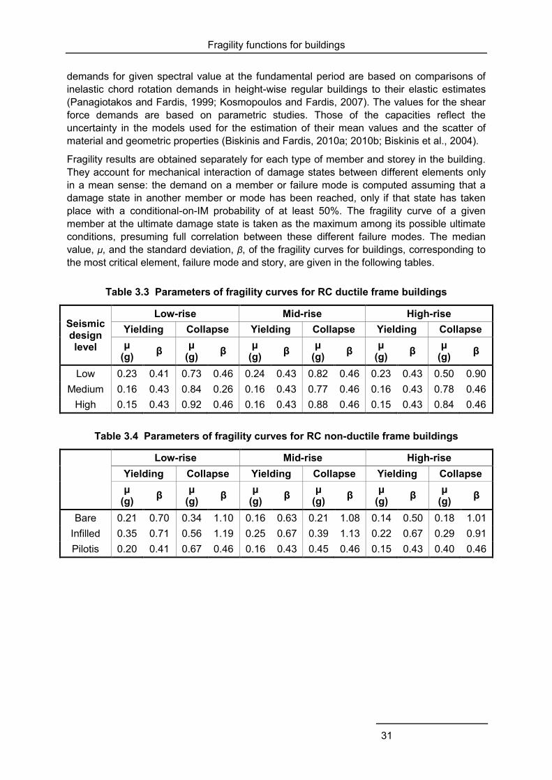
Fragility functions for buildings
31
demands for given spectral value at the fundamental period are based on comparisons of inelastic chord rotation demands in height-wise regular buildings to their elastic estimates (Panagiotakos and Fardis, 1999; Kosmopoulos and Fardis, 2007). The values for the shear force demands are based on parametric studies. Those of the capacities reflect the uncertainty in the models used for the estimation of their mean values and the scatter of material and geometric properties (Biskinis and Fardis, 2010a; 2010b; Biskinis et al., 2004).
Fragility results are obtained separately for each type of member and storey in the building. They account for mechanical interaction of damage states between different elements only in a mean sense: the demand on a member or failure mode is computed assuming that a damage state in another member or mode has been reached, only if that state has taken place with a conditional-on-IM probability of at least 50%. The fragility curve of a given member at the ultimate damage state is taken as the maximum among its possible ultimate conditions, presuming full correlation between these different failure modes. The median value, μ, and the standard deviation, β, of the fragility curves for buildings, corresponding to the most critical element, failure mode and story, are given in the following tables.
Table 3.3 Parameters of fragility curves for RC ductile frame buildings
Seismic design level
Low-rise Mid-rise High-rise Yielding Collapse Yielding Collapse Yielding Collapse μ
(g) β μ (g) β μ
(g) β μ (g) β μ
(g) β μ (g) β
Low 0.23 0.41 0.73 0.46 0.24 0.43 0.82 0.46 0.23 0.43 0.50 0.90 Medium 0.16 0.43 0.84 0.26 0.16 0.43 0.77 0.46 0.16 0.43 0.78 0.46
High 0.15 0.43 0.92 0.46 0.16 0.43 0.88 0.46 0.15 0.43 0.84 0.46
Table 3.4 Parameters of fragility curves for RC non-ductile frame buildings
Low-rise Mid-rise High-rise Yielding Collapse Yielding Collapse Yielding Collapse μ
(g) β μ (g) β μ
(g) β μ (g) β μ
(g) β μ (g) β
Bare 0.21 0.70 0.34 1.10 0.16 0.63 0.21 1.08 0.14 0.50 0.18 1.01 Infilled 0.35 0.71 0.56 1.19 0.25 0.67 0.39 1.13 0.22 0.67 0.29 0.91 Pilotis 0.20 0.41 0.67 0.46 0.16 0.43 0.45 0.46 0.15 0.43 0.40 0.46

Fragility functions for buildings
32
Table 3.5 Parameters of fragility curves for RC wall buildings
Seismic design level
Mid-rise High-rise Yielding Collapse Yielding Collapse μ
(g) β μ (g) β μ
(g) β μ (g) β
None 0.09 0.52 0.17 0.22 0.08 0.36 0.15 0.15 Low 0.12 0.37 0.17 0.22 0.11 0.36 0.17 0.20
Medium 0.13 0.38 0.18 0.21 0.11 0.38 0.18 0.18 High 0.16 0.49 0.42 0.24 0.15 0.50 0.29 0.21
Table 3.6 Parameters of fragility curves for RC dual buildings
Seismic design level
Mid-rise High-rise Yielding Collapse Yielding Collapse μ
(g) β μ (g) β μ
(g) β μ (g) β
Low 0.11 0.38 0.22 0.12 0.12 0.49 0.33 0.17 Medium 0.11 0.50 0.19 0.20 0.09 0.50 0.33 0.44
High 0.12 0.49 0.39 0.22 0.15 0.48 0.38 0.20
3.2.2 Fragility curves for stone masonry buildings based on FE analysis
Out-of-plane behaviour affects to a large extent the seismic response of old masonry buildings with flexible floors, and modelling by means of equivalent planar frames is not able to capture this failure mode. New fragility curves were produced for stone masonry buildings that consider both in-plane and out-of-plane response and failure modes, using three-dimensional analysis with finite element modelling and a nonlinear biaxial failure criterion.
216 prototype regular buildings are analysed, so as to cover the practical range of the following parameters: number of storeys, percentage of side length in external walls taken up by openings, wall thickness, plan dimensions, floor type and wall height-to-length ratio.
The five damage grades of the European Macroseismic Scale (Grünthal 1998) are used. The damage measure is a function of the percentage and the location of the surface area of the wall faces where failure of the masonry takes place according to a nonlinear biaxial failure criterion based on the stresses at the two faces of the masonry wall (Karantoni et al., 1993). The criterion is an extension of a four-parameter model for the failure of concrete under triaxial stresses (Ottosen, 1977).
An effective spectral acceleration, Sa,eff = 2.5αg/q(DG), is adopted as intensity measure, where αg is the peak ground acceleration of the earthquake input (in g) and q(DG) an effective behaviour factor that accounts for the different levels of damping associated to each damage grade (DG). Damage grade 1 corresponds to (almost) elastic response, thus the behaviour factor is q(1) = 1. A basic value of the behaviour factor qRo(5) = 2.0 is adopted for buildings with rigid floors. It is multiplied by an overstrength factor αu/α1 = 2.0, to account for the actual behaviour after the first structural element fails (Magenes, 2006), resulting in qR(5) = 4.0. Buildings with flexible floors are expected to reach damage grade 5 with less
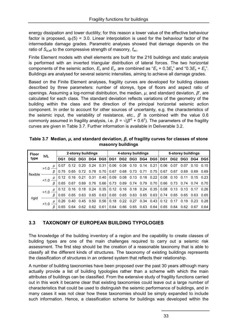
Fragility functions for buildings
33
energy dissipation and lower ductility; for this reason a lower value of the effective behaviour factor is proposed, qF(5) = 3.0. Linear interpolation is used for the behaviour factor of the intermediate damage grades. Parametric analyses showed that damage depends on the ratio of Sa,eff to the compressive strength of masonry, fwc.
Finite Element models with shell elements are built for the 216 buildings and static analysis is performed with an inverted triangular distribution of lateral forces. The two horizontal components of the seismic action, Ex and Ey, are combined as “Ex + 0.3Ey” and “0.3Ex + Ey”. Buildings are analysed for several seismic intensities, aiming to achieve all damage grades.
Based on the Finite Element analyses, fragility curves are developed for building classes described by three parameters: number of storeys, type of floors and aspect ratio of openings. Assuming a log-normal distribution, the median, μ, and standard deviation, β', are calculated for each class. The standard deviation reflects variations of the geometry of the building within the class and the direction of the principal horizontal seismic action component. In order to account for other sources of uncertainty, e.g. the characteristics of the seismic input, the variability of resistance, etc., β' is combined with the value 0.6 commonly assumed in fragility analysis, i.e. β = √(β'2 + 0.62). The parameters of the fragility curves are given in Table 3.7. Further information is available in Deliverable 3.2.
Table 3.7 Median, μ, and standard deviation, β, of fragility curves for classes of stone masonry buildings
Floor type h/L
2-storey buildings 4-storey buildings 6-storey buildings DG1 DG2 DG3 DG4 DG5 DG1 DG2 DG3 DG4 DG5 DG1 DG2 DG3 DG4 DG5
flexible >1.0
μ 0.07 0.12 0.20 0.24 0.31 0.06 0.08 0.10 0.14 0.21 0.06 0.07 0.07 0.10 0.15 β 0.75 0.65 0.72 0.78 0.70 0.67 0.68 0.73 0.71 0.75 0.67 0.67 0.69 0.69 0.69
<1.0 μ 0.12 0.16 0.21 0.31 0.40 0.09 0.08 0.13 0.18 0.22 0.08 0.10 0.11 0.15 0.23 β 0.65 0.67 0.69 0.76 0.66 0.73 0.69 0.74 0.79 0.70 0.66 0.73 0.74 0.74 0.70
rigid >1.0
μ 0.12 0.16 0.18 0.24 0.35 0.12 0.16 0.18 0.24 0.35 0.08 0.13 0.13 0.17 0.26 β 0.65 0.65 0.63 0.65 0.63 0.65 0.65 0.63 0.65 0.63 0.74 0.65 0.65 0.63 0.65
<1.0 μ 0.26 0.40 0.45 0.50 0.56 0.18 0.22 0.27 0.34 0.43 0.12 0.17 0.19 0.23 0.28 β 0.65 0.64 0.62 0.62 0.61 0.64 0.66 0.65 0.63 0.64 0.65 0.64 0.62 0.67 0.64
3.3 TAXONOMY OF EUROPEAN BUILDING TYPOLOGIES
The knowledge of the building inventory of a region and the capability to create classes of building types are one of the main challenges required to carry out a seismic risk assessment. The first step should be the creation of a reasonable taxonomy that is able to classify all the different kinds of structures. The taxonomy of existing buildings represents the classification of structures in an ordered system that reflects their relationship.
A number of building taxonomies have been proposed over the past 30 years although many actually provide a list of building typologies rather than a scheme with which the main attributes of buildings can be classified. From the extensive study of fragility functions carried out in this work it became clear that existing taxonomies could leave out a large number of characteristics that could be used to distinguish the seismic performance of buildings, and in many cases it was not clear how these taxonomies should be simply expanded to include such information. Hence, a classification scheme for buildings was developed within the
Fragility functions for buildings
34
SYNER-G project; this taxonomy was defined by Charleson (2011) as having the most potential amongst all taxonomies reviewed and subsequently formed the basis of the Global Earthquake Model (GEM) Basic Building Taxonomy (Brzev et al., 2012). The main categories of this classification scheme proposed for buildings within SYNER-G (see SYNER-G Reference Report 2, Chapter 3) are: force resisting mechanism, force resisting mechanism material, plan regularity, elevation regularity, cladding, detailing, floor system, roof system, height level, and code level.
3.4 HARMONISATION OF FRAGILITY FUNCTIONS
The harmonisation of European fragility functions for buildings has been tackled within the SYNER-G project. As mentioned above, in the reviewed papers, different Intensity Measure Types have been used to describe the level of ground shaking and a different number of limit states has been adopted according to the damage scale used. For the purpose of comparing all the different existing studies and fragility functions, harmonisation is an essential step. To compare different curves, the same intensity measure types, the same number of limit states and the same building typology is needed.
For this latter reason, there are three main steps that have to be followed in the harmonisation process:
1. Harmonisation of the intensity measure types;
2. Harmonisation of limit states;
3. Harmonisation of the building typology.
In the following paragraphs these phases are described in detail.
3.4.1 Harmonisation of intensity measure types
All the intensity measure types have been converted into PGA due to the ease with which it can be used in seismic risk assessment, and the fact that it was already being used in the majority of the studies considered (see Figure 3.4). There are a number of different conversion equations that allow IMTs (such as PGV, MMI) to be converted to peak ground acceleration and some recommendations have been made in the selection of some of these considering the fact that the region of interest is Europe and considering recent research (Cua et al., 2010). For further details, the reader is referred to SYNER-G Deliverables 3.1 and 3.2.It is noted that there is a large variability between macroseismic and instrumental intensity measures, and such uncertainty has not yet been considered within the tool; thus, only the mean relationship between these two parameters has been considered.
It has not been possible to convert all the different intensity measure types found in the reviewed papers due to some shortcomings or lack of conversion equations, and in some cases there are large uncertainties involved in such conversions. For example, the conversion of Sd(TLS) to PGA would require knowledge of the inelastic period and equivalent viscous damping at the limit state that was considered in the non-linear analyses. Nevertheless, the majority of the fragility functions can be harmonised and the following IMTs have been converted to PGA: macroseismic Intensity, Sa(Ty), Sd(Ty) and PGV. The Fragility Function Manager tool allows the user to choose from the available equations to convert the IMT to PGA, and to assign values for the yield period of vibration.
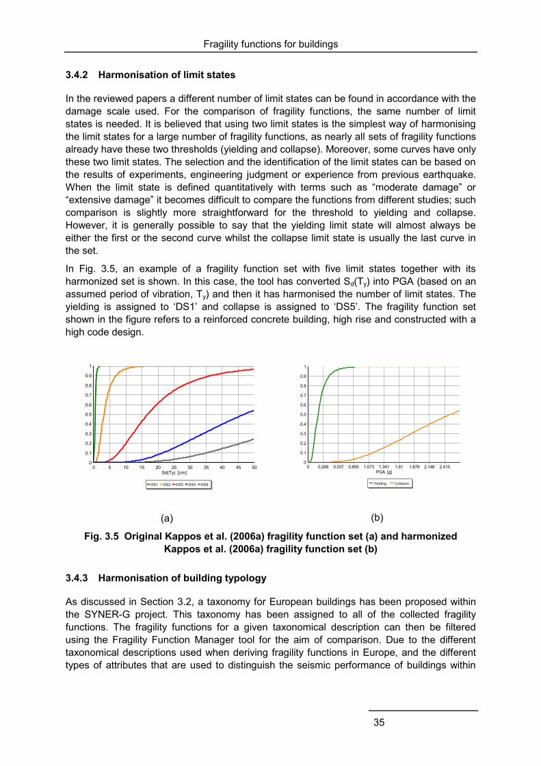
Fragility functions for buildings
35
3.4.2 Harmonisation of limit states
In the reviewed papers a different number of limit states can be found in accordance with the damage scale used. For the comparison of fragility functions, the same number of limit states is needed. It is believed that using two limit states is the simplest way of harmonising the limit states for a large number of fragility functions, as nearly all sets of fragility functions already have these two thresholds (yielding and collapse). Moreover, some curves have only these two limit states. The selection and the identification of the limit states can be based on the results of experiments, engineering judgment or experience from previous earthquake. When the limit state is defined quantitatively with terms such as “moderate damage” or “extensive damage” it becomes difficult to compare the functions from different studies; such comparison is slightly more straightforward for the threshold to yielding and collapse. However, it is generally possible to say that the yielding limit state will almost always be either the first or the second curve whilst the collapse limit state is usually the last curve in the set.
In Fig. 3.5, an example of a fragility function set with five limit states together with its harmonized set is shown. In this case, the tool has converted Sd(Ty) into PGA (based on an assumed period of vibration, Ty) and then it has harmonised the number of limit states. The yielding is assigned to ‘DS1’ and collapse is assigned to ‘DS5’. The fragility function set shown in the figure refers to a reinforced concrete building, high rise and constructed with a high code design.
(a)
(b)
Fig. 3.5 Original Kappos et al. (2006a) fragility function set (a) and harmonized Kappos et al. (2006a) fragility function set (b)
3.4.3 Harmonisation of building typology
As discussed in Section 3.2, a taxonomy for European buildings has been proposed within the SYNER-G project. This taxonomy has been assigned to all of the collected fragility functions. The fragility functions for a given taxonomical description can then be filtered using the Fragility Function Manager tool for the aim of comparison. Due to the different taxonomical descriptions used when deriving fragility functions in Europe, and the different types of attributes that are used to distinguish the seismic performance of buildings within
DS1 DS2 DS3 DS4 DS5
Sd(Ty) [cm]50454035302520151050
Pro
babi
lity
of e
xcee
danc
e
1
0.9
0.8
0.7
0.6
0.5
0.4
0.3
0.2
0.1
0
Yielding Collapse
PGA [g]2.4152.1461.8781.611.3411.0730.8050.5370.2680
Pro
babi
lity
of e
xcee
danc
e
1
0.9
0.8
0.7
0.6
0.5
0.4
0.3
0.2
0.1
0

Fragility functions for buildings
36
these different studies, a reduced number of attributes has been used for the purposes of comparing fragility functions, as described below.
Fig. 3.6 is presented as an example to illustrate the building typologies for which fragility functions of reinforced concrete can be compared. Each column represents a different and additional attribute. Fragility functions can be compared by taking into account different levels of attributes. For instance, all the available fragility functions sets concerning reinforced concrete with moment resisting frame building that are low rise (of which there are 25) can be compared, or all the available fragility functions sets concerning reinforced concrete with moment resisting frame buildings that are low rise, seismically designed, bare and ductile (of which there are 6). As can be seen, the attributes of plan regularity, elevation regularity, floor system and roof system are not used in this plot as few fragility functions have classified the reinforced concrete buildings using these attributes.
Figure 3.6 also provides a summary of building classes for which there are few fragility functions and which should be analysed in future research developments; these include high rise moment resisting frames (MRF) with seismic design and infills, and frame-wall structures without seismic design were much less common than their seismically designed counterparts. In fact, there are some classes that are represented by very few fragility curves (sometimes just one fragility function), and for this reason it is not possible to conduct a critical review and an exhaustive study of the uncertainties for these building types.
On the other hand, the available fragility function sets for the class of masonry buildings are shown in Fig. 3.7. In this case the fragility functions could be compared by taking into account just the material or also the height level. Not all attributes of the taxonomy have been used for the comparison of fragility functions for masonry buildings because in most cases this would lead to very few fragility functions. In particular, plan regularity, elevation regularity, cladding, detailing, floor system, roof system, and code level have not been used for the comparisons herein, even though it is possible to find some fragility functions that do use these attributes to classify the buildings. It has to be noted that a few studies have dealt with the out of plane mechanism for masonry buildings, and it is possible to compare only a limited number of fragility curves. There is certainly a need for this mechanism to be further studied in future European fragility function research. In the next section of this report a methodology for comparing fragility functions is presented.
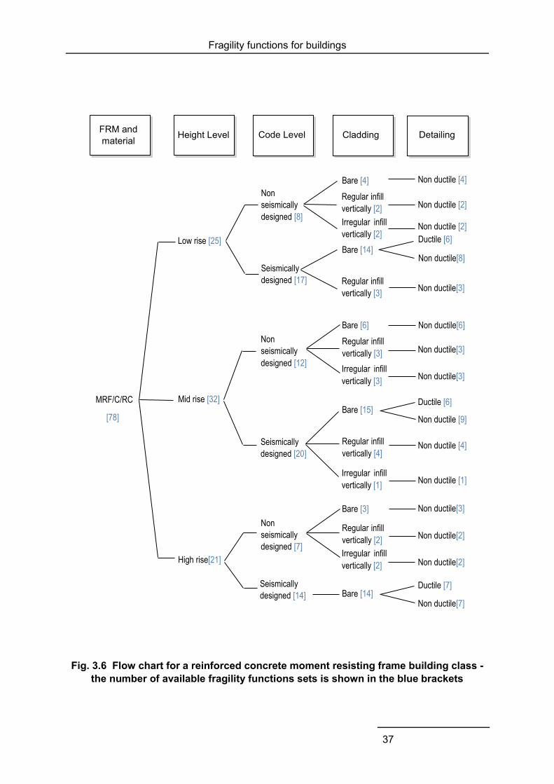
Fragility functions for buildings
37
Fig. 3.6 Flow chart for a reinforced concrete moment resisting frame building class -
the number of available fragility functions sets is shown in the blue brackets
FRM and material Height Level Code Level Detailing Cladding
MRF/C/RC
[78]
Non ductile [2]
Bare [4]
Non
seismically
designed [8]
Ductile [6]
Non ductile[8] Seismically
designed [17]
Bare [14]
Regular infill
vertically [3] Non ductile[3]
Low rise [25]
Non ductile[6]
Non ductile[3]
Non ductile[3]
Bare [6]
Regular infill
vertically [3]
Irregular infill
vertically [3]
Non
seismically
designed [12]
Ductile [6]
Non ductile [9]
Non ductile [4]
Bare [15]
Regular infill
vertically [4]
Irregular infill
vertically [1]
Seismically
designed [20]
Mid rise [32]
Non ductile[3] Bare [3]
Non
seismically
designed [7]
Ductile [7]
Non ductile[7] Bare [14]
Seismically
designed [14]
High rise[21]
Non ductile [4]
Regular infill
vertically [2]
Irregular infill
vertically [2] Non ductile [2]
Non ductile [1]
Regular infill
vertically [2] Non ductile[2]
Non ductile[2] Irregular infill
vertically [2]
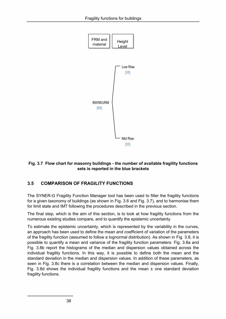
Fragility functions for buildings
38
Fig. 3.7 Flow chart for masonry buildings - the number of available fragility functions
sets is reported in the blue brackets
3.5 COMPARISON OF FRAGILITY FUNCTIONS
The SYNER-G Fragility Function Manager tool has been used to filter the fragility functions for a given taxonomy of buildings (as shown in Fig. 3.6 and Fig. 3.7), and to harmonise them for limit state and IMT following the procedures described in the previous section.
The final step, which is the aim of this section, is to look at how fragility functions from the numerous existing studies compare, and to quantify the epistemic uncertainty.
To estimate the epistemic uncertainty, which is represented by the variability in the curves, an approach has been used to define the mean and coefficient of variation of the parameters of the fragility function (assumed to follow a lognormal distribution). As shown in Fig. 3.8, it is possible to quantify a mean and variance of the fragility function parameters: Fig. 3.8a and Fig. 3.8b report the histograms of the median and dispersion values obtained across the individual fragility functions. In this way, it is possible to define both the mean and the standard deviation in the median and dispersion values. In addition of these parameters, as seen in Fig. 3.8c there is a correlation between the median and dispersion values. Finally, Fig. 3.8d shows the individual fragility functions and the mean ± one standard deviation fragility functions.
BW/M/URM
Low Rise
Mid Rise
FRM and material
Height Level
[69]
[38]
[35]
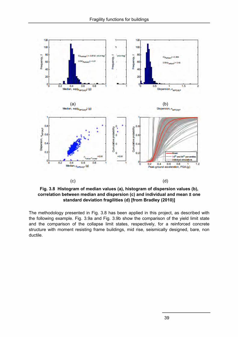
Fragility functions for buildings
39
(a) (b)
(c) (d)
Fig. 3.8 Histogram of median values (a), histogram of dispersion values (b), correlation between median and dispersion (c) and individual and mean ± one
standard deviation fragilities (d) [from Bradley (2010)]
The methodology presented in Fig. 3.8 has been applied in this project, as described with the following example. Fig. 3.9a and Fig. 3.9b show the comparison of the yield limit state and the comparison of the collapse limit states, respectively, for a reinforced concrete structure with moment resisting frame buildings, mid rise, seismically designed, bare, non ductile.
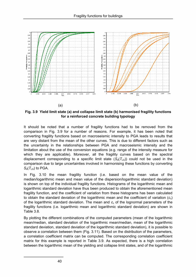
Fragility functions for buildings
40
(a)
(b)
Fig. 3.9 Yield limit state (a) and collapse limit state (b) harmonised fragility functions for a reinforced concrete building typology
It should be noted that a number of fragility functions had to be removed from the comparison in Fig. 3.9 for a number of reasons. For example, it has been noted that converting fragility functions based on macroseismic intensity to PGA leads to results that are very distant from the mean of the other curves. This is due to different factors such as the uncertainty in the relationships between PGA and macroseismic intensity and the limitation about the use of the conversion equations (e.g. range of the intensity measure for which they are applicable). Moreover, all the fragility curves based on the spectral displacement corresponding to a specific limit state (Sd(TLS)) could not be used in the comparison due to large uncertainties involved in harmonising these functions by converting Sd(TLS) to PGA.
In Fig. 3.10 the mean fragility function (i.e. based on the mean value of the median/logarithmic mean and mean value of the dispersion/logarithmic standard deviation) is shown on top of the individual fragility functions. Histograms of the logarithmic mean and logarithmic standard deviation have thus been produced to obtain the aforementioned mean fragility function, and the coefficient of variation from these histograms has been calculated to obtain the standard deviation of the logarithmic mean and the coefficient of variation (cv) of the logarithmic standard deviation. The mean and cv of the lognormal parameters of the fragility functions (i.e. logarithmic mean and logarithmic standard deviation) are shown in Table 3.8.
By plotting the different combinations of the computed parameters (mean of the logarithmic mean/median, standard deviation of the logarithmic mean/median, mean of the logarithmic standard deviation, standard deviation of the logarithmic standard deviation), it is possible to observe a correlation between them (Fig. 3.11). Based on the distribution of the parameters, a correlation coefficient matrix can be computed. The corresponding correlation coefficient matrix for this example is reported in Table 3.9. As expected, there is a high correlation between the logarithmic mean of the yielding and collapse limit states, and of the logarithmic

Fragility functions for buildings
41
standard deviation of these two limit states. On the other hand, very little correlation is observed between the logarithmic means and the logarithmic standard deviations.
Fig. 3.10 Mean fragility function for (a) limit state yielding curve and (b) limit state
collapse curve for a reinforced concrete building typology
Table 3.8 Mean and coefficient of variation, cv, of lognormal fragility parameters for a reinforced concrete building typology
Reinforced Concrete – Mid Rise, Seismically Designed, Bare and Non Ductile Yielding Collapse Logarithmic
Mean, μ1 Logarithmic Standard
Deviation, σ1 Logarithmic
Mean, μ2 Logarithmic Standard
Deviation, σ2 Mean -1.832 0.474 -1.091 0.485 cv (%) 33 21 48 24
Fig. 3.11 Correlation between individual fragility functions parameters

Fragility functions for buildings
42
Table 3.9 Correlation coefficient matrix for a reinforced concrete building typology
μ1 σ1 μ2 σ2
μ1 1 0.158 0.783 0.033 σ1 0.158 1 0.118 0.614 μ2 0.783 0.118 1 -0.453 σ2 0.033 0.614 -0.453 1
The mean and coefficient of variation of the parameters of the lognormal distribution for the yielding and collapse limit state for a number of building typologies, based on the fragility functions reviewed in this study, are presented in Appendix A.
Fragility functions for utility networks
43
4 Fragility functions for utility networks
4.1 ELECTRIC POWER NETWORK
4.1.1 Identification of main typologies
A modern EPN (Electric Power Network) is a complex interconnected system designed to generate, transform and transfer electric energy from generating units at various locations to the customers demanding the loads, which can be of different types (industrial, commercial and residential).The electric power systems components can be grouped on the basis of four different analysis levels of the network. The main typologies, with particular reference to the European context, are listed in Table 4.1. It has been noted from the literature review that authors often assign different names to the same micro-component.
It has to be remarked that most authors do not explicitly distinguish between micro- and macro-components. This distinction is useful in terms of reliability analysis when the approach to network modelling is capacitive (i.e. power flows are computed) and the internal logic of substations is modelled, i.e., partial functioning (continued service with reduced power flow) is accounted for. In the latter case, the modelling effort that is much higher than when a substation is considered as a single component with a binary state (fail/safe), can be reduced by assembling sub-sets of micro-components that are serially arranged within the substation in order to reduce them to a single element characterised by a single fragility: the macro-component. The substation layout is then composed of a general (non-serial) arrangement of macro-components which can lead to partial functioning states, depending on the distribution of damage.
Looking again to Table 4.1, it should be clear how some of the components listed, for which a fragility curve/model could be retrieved in the literature (as reported in Section 4.1.2), are not of interest within the SYNER-G analysis framework where the level of detail/ resolution in the description of the EPN, and in general of lifelines, is higher. In particular, a fragility model for the whole network (EPN01) cannot be used, and a fragility model for an entire substation (EPN03) can only be used in preliminary simplified connectivity-only analyses.
4.1.2 State of the art fragility functions for electric power system components
Table 4.2 reports the main recent works on fragility functions of electric power system components, with the indication of the methodology used to evaluate the curves, the components classification, the considered intensity measure, as well as damage states and indices.
Deliverable 3.3 contains a number of tables reporting the details about the fragility functions related to the different EPN components’ typologies and extracted from the works listed in Table 4.2. The tables are grouped in three sections, the first of which is related to the whole network and the stations, while the remaining two sections deal with macro- and micro-components fragility curves. It has to be remarked here that the fragility curves for electric power grids are not of interest for SYNER-G, since the aim is to perform a fragility

Fragility functions for utility networks
44
assessment of lifelines, and in particular of an EPN at a lower analysis level, from the micro-component up to the station, including also the distribution circuits.
Several of the surveyed works do not report numerical parameters for the fragility curves. Given the importance of having the parameters for using these models in an infrastructure simulation analysis, in this report these parameters have been approximately determined from quintile values graphically retrieved from the curves. In particular, this has been done in different ways.
Table 4.1 Main typologies of EPN components in Europe
Typology Analysis level Element code Electric power grid Network EPN01 Generation plant Station EPN02 Substation Station EPN03 Distribution circuits Distribution-system EPN04 Macro-components Substation’s component Autotransformer line Substation’s component EPN05 Line without transformer Substation’s component EPN06 Bars-connecting line Substation’s component EPN07 Bars Substation’s component EPN08 Cluster Substation’s component EPN09 Micro-components Substation’s component Circuit breaker Substation’s component EPN10 Lightning arrester or Discharger Substation’s component EPN11
Horizontal disconnect switch or Horizontal sectionalizing switch Substation’s component EPN12
Vertical disconnect switch or Vertical sectionalizing switch Substation’s component EPN13
Transformer or Autotransformer Substation’s component EPN14 Current transformer Substation’s component EPN15 Voltage transformer Substation’s component EPN16 Box or Control house Substation’s component EPN17 Power supply to protection system Substation’s component EPN18 Coil support Substation’s component EPN19 Bar support or Pothead Substation’s component EPN20 Regulator Substation’s component EPN21 Bus Substation’s component EPN22 Capacitor bank Substation’s component EPN23

Fragility functions for utility networks
45
Table 4.2 Main works on fragilities of EPN components
Reference Methodology Elements classification IMT Damage States
and Indices
Anagnos, 1999 Empirical, with
two normal functions
6 electric micro-components
Peak Ground
Acceleration
Failure with different failure
modes depending on the considered
component
Anagnos and Ostrom, 2000
Empirical, with two normal functions
500 kV circuit breaker and 230
kV horizontal disconnect switch
Peak Ground
Acceleration
Failure with different failure
modes depending on the considered
component
Anget al.,1996 Empirical, with
lognormal function
6 electric micro-components and 500 kV-230 kV
substations
Peak Ground
Acceleration
Failure based on power imbalance, abnormal voltage, unstable condition
and operational power interruption
Bettinali et al.,2004 Numerical 11 electric micro-
components
Peak Ground
Acceleration Failure
Dueñas-Osorio et al., 2007
Empirical, with lognormal function
Electric power grid Peak
Ground Acceleration
Failure based on substation
functionality; CL1 = 20, 50 and
80%
FEMA – HAZUSMH Technical
Manual, 2003
Numerical, Boolean approach
Substation, distribution circuits,
generation plant and 4 micro-components
Peak Ground
Acceleration
Slight/minor; Moderate; Extensive; Complete
Giovinazzi and King, 2009
Empirical (lognormal function)/ Numerical
Medium voltage substation
Peak Ground
Acceleration
Slight/minor; Moderate; Extensive; Complete
Hwang and Huo,1998
Empirical (lognormal function)/ Numerical
9 electric micro-components,
pothead structure and 115/12 kV
transformer
Peak Ground
Acceleration Failure
Hwang and Chou, 1998
Numerical, dynamic
analyses, fault tree
6 electric micro-components, 1
macro-component and substation
Peak Ground
Acceleration Failure
Liu et al.,2003 Empirical, with
two normal functions
500 kV- 230 kV three-phase transformers
Peak Ground
Acceleration Failure
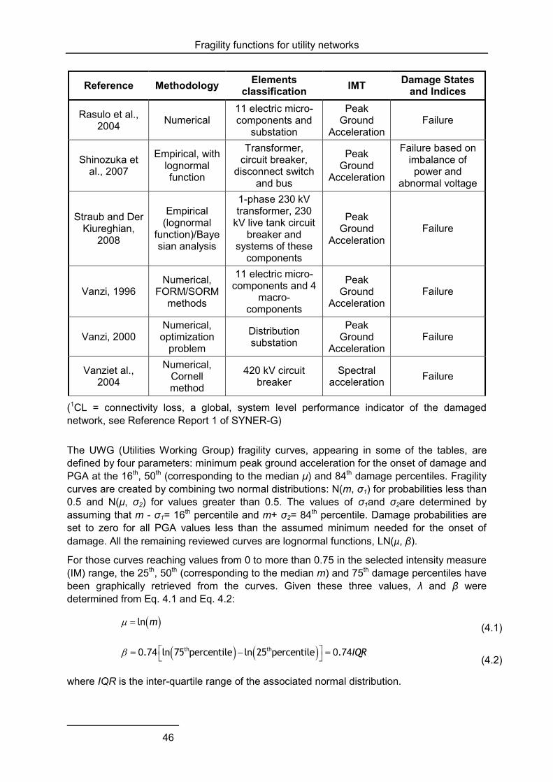
Fragility functions for utility networks
46
Reference Methodology Elements classification IMT Damage States
and Indices
Rasulo et al., 2004 Numerical
11 electric micro-components and
substation
Peak Ground
Acceleration Failure
Shinozuka et al., 2007
Empirical, with lognormal function
Transformer, circuit breaker,
disconnect switch and bus
Peak Ground
Acceleration
Failure based on imbalance of power and
abnormal voltage
Straub and Der Kiureghian,
2008
Empirical (lognormal
function)/Bayesian analysis
1-phase 230 kV transformer, 230
kV live tank circuit breaker and
systems of these components
Peak Ground
Acceleration Failure
Vanzi, 1996 Numerical,
FORM/SORM methods
11 electric micro-components and 4
macro-components
Peak Ground
Acceleration Failure
Vanzi, 2000 Numerical, optimization
problem
Distribution substation
Peak Ground
Acceleration Failure
Vanziet al., 2004
Numerical, Cornell method
420 kV circuit breaker
Spectral acceleration Failure
(1CL = connectivity loss, a global, system level performance indicator of the damaged network, see Reference Report 1 of SYNER-G)
The UWG (Utilities Working Group) fragility curves, appearing in some of the tables, are defined by four parameters: minimum peak ground acceleration for the onset of damage and PGA at the 16th, 50th (corresponding to the median μ) and 84th damage percentiles. Fragility curves are created by combining two normal distributions: N(m, σ1) for probabilities less than 0.5 and N(μ, σ2) for values greater than 0.5. The values of σ1and σ2are determined by assuming that m - σ1= 16th percentile and m+ σ2= 84th percentile. Damage probabilities are set to zero for all PGA values less than the assumed minimum needed for the onset of damage. All the remaining reviewed curves are lognormal functions, LN(μ, β).
For those curves reaching values from 0 to more than 0.75 in the selected intensity measure (IM) range, the 25th, 50th (corresponding to the median m) and 75th damage percentiles have been graphically retrieved from the curves. Given these three values, λ and β were determined from Eq. 4.1 and Eq. 4.2:
ln m (4.1)
th th. ln 75 percentile ln 25 percentile . IQR
0 74 0 74 (4.2)
where IQR is the inter-quartile range of the associated normal distribution.

Fragility functions for utility networks
47
For the few remaining curves, β was computed with different expressions depending on the case. These are all similar to Eq. 4.2 in which the 25th and 75th damage percentiles were replaced by two available percentile values, while 0.74 was replaced by a coefficient numerically obtained from normal random sampling. The λ parameter was determined as in Eq. 4.1, with the m value read from the curve if possible, otherwise assumed in a way that the approximate curve, with a fixed value of the β parameter, was as close as possible to the original one.
The entry “Method” appearing in the tables, reports the method employed to derive the fragility curves:
o empirical: statistical regression on data from damage surveys in actual events, or from laboratory test;
o numerical: using response data from numerical simulations of the component under earthquake input.
4.1.3 Proposal of standard damage scales
This section proposes standard damage scales for EPN components. For each of the main typologies, the different damage states are related to the serviceability of the whole network or the single station, depending on the considered analysis level. In particular, for the network and distribution-system levels, the tables refer to the serviceability of the single station.
The damage scales below do not quantify the reduction of power flow corresponding to each damage state. Actually, the performance of the network and even of a single station cannot be predicted without a power flow analysis, continued serviceability resulting from the interaction between various components, both inside the individual station and within the neighbouring ones, as well as from the spread of short circuits to other parts of the station and to the remaining parts of the network.
Damage scales for electric power grids
The paper by Dueñas-Osorio presents fragility curves related to the whole electric power grid composed of different types of stations, transmission and distribution lines. Two damage scales are proposed for electric power grids and reported in Table 4.3 and Table 4.4, differing for the damage state definition. It should be noted how the definition of nominal and reduced power flow is not quantitative and, hence, not operational.
Table 4.3 Damage scale for electric power grids: first proposal
Serviceability Damage State description
No power available
Operational after long term
repairs Extensive
This limit state implies damage beyond short-term repair, leaving the network systems under consideration as completely non-functional.
Nominal power flow
Operational without repair None None
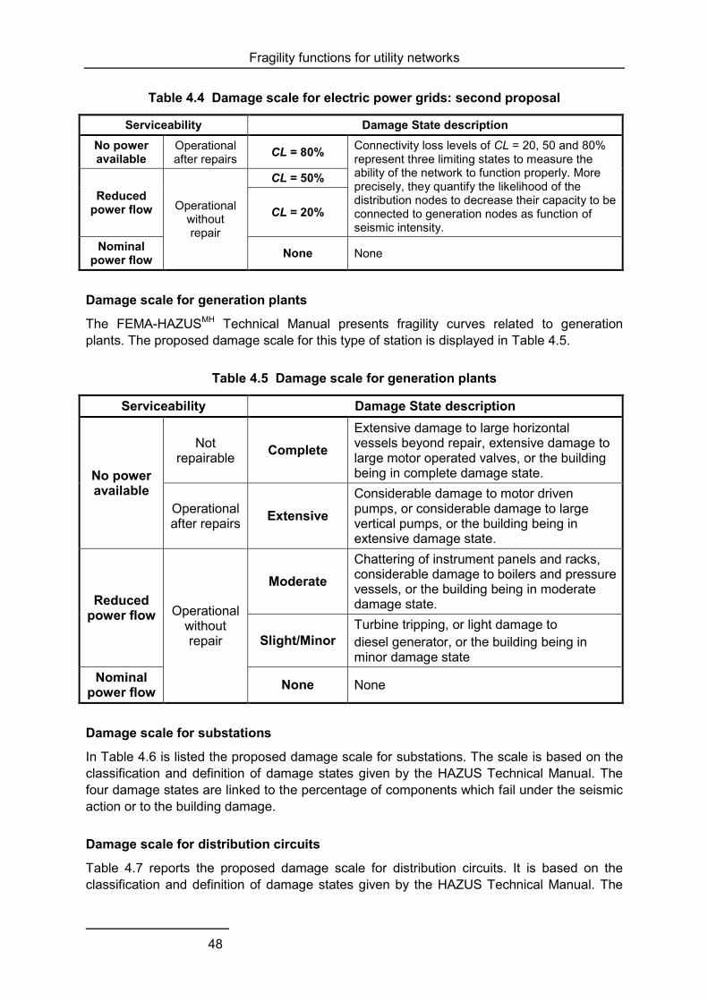
Fragility functions for utility networks
48
Table 4.4 Damage scale for electric power grids: second proposal
Serviceability Damage State description No power available
Operational after repairs CL = 80% Connectivity loss levels of CL = 20, 50 and 80%
represent three limiting states to measure the ability of the network to function properly. More precisely, they quantify the likelihood of the distribution nodes to decrease their capacity to be connected to generation nodes as function of seismic intensity.
Reduced power flow Operational
without repair
CL = 50%
CL = 20%
Nominal power flow None None
Damage scale for generation plants
The FEMA-HAZUSMH Technical Manual presents fragility curves related to generation plants. The proposed damage scale for this type of station is displayed in Table 4.5.
Table 4.5 Damage scale for generation plants
Serviceability Damage State description
No power available
Not repairable Complete
Extensive damage to large horizontal vessels beyond repair, extensive damage to large motor operated valves, or the building being in complete damage state.
Operational after repairs Extensive
Considerable damage to motor driven pumps, or considerable damage to large vertical pumps, or the building being in extensive damage state.
Reduced power flow Operational
without repair
Moderate Chattering of instrument panels and racks, considerable damage to boilers and pressure vessels, or the building being in moderate damage state.
Slight/Minor Turbine tripping, or light damage to diesel generator, or the building being in minor damage state
Nominal power flow None None
Damage scale for substations
In Table 4.6 is listed the proposed damage scale for substations. The scale is based on the classification and definition of damage states given by the HAZUS Technical Manual. The four damage states are linked to the percentage of components which fail under the seismic action or to the building damage.
Damage scale for distribution circuits
Table 4.7 reports the proposed damage scale for distribution circuits. It is based on the classification and definition of damage states given by the HAZUS Technical Manual. The

Fragility functions for utility networks
49
four damage states are linked to the percentage of circuits which fail under the seismic action.
Table 4.6 Damage scale for substations
Serviceability Damage State description
No power available
Not repairable Complete
Failure of all disconnected switches, all circuit breakers, all transformers, or all current transformers, or the building being in complete damage state.
Operational after repairs Extensive
Failure of 70% of disconnect switches (e.g., misalignment), 70% of circuit breakers, 70% of current transformers (e.g., oil leaking from transformers, porcelain cracked), or failure of 70% of transformers (e.g., leakage of transformer radiators), or the building being in extensive damage state.
Reduced power flow Operational
without repair
Moderate
Failure of 40% of disconnect switches (e.g., misalignment), or 40% of circuit breakers (e.g., circuit breaker phase sliding off its pad, circuit breaker tipping over, or interrupter-head falling to the ground), or failure of 40% of current transformers (e.g., oil leaking from transformers, porcelain cracked), or the building being in moderate damage state.
Slight/Minor
Failure of 5% of the disconnect switches (i.e., misalignment), or failure of 5% of the circuit breakers (i.e., circuit breaker phase sliding off its pad, circuit breaker tipping over, or interrupter-head falling to the ground), or the building being in minor damage state.
Nominal power flow None None
Table 4.7 Damage scale for distribution circuits
Serviceability Damage State description
No power available
Not repairable Complete Failure of 80% of all circuits
Operational after repairs Extensive Failure of 50% of all circuits
Reduced power flow Operational
without repair
Moderate Failure of 12% of all circuits
Slight/Minor Failure of 4% of all circuits Nominal
power flow None None
Damage scales for macro-components
Table 4.8, Table 4.9 and Table 4.10 present the proposed damage scales for electric macro-components, according to their definitions given in the study by (Vanzi, 1996) and (Hwang

Fragility functions for utility networks
50
and Chou, 1998) and reported below for reference. All macro-components are considered as series systems of several micro-components. The failure of some macro-components involves the failure of the entire substation, since they constitute the minimal cut sets of the system. The failure of some other macro-components only involves a reduction of the power flow outgoing from the substation.
1. Autotransformer line (autotransformer + dischargers + current transformers + circuit breakers + bearings)
2. Line without transformer (voltage transformer + coil support + sectionalizing switch + current transformer + circuit breaker + bearings)
3. Bars-connecting line (sectionalizing switch + current transformer + circuit breaker + bearings
4. Bars (voltage transformer + bearings)
5. Cluster (pothead, 6 lightning arresters, 115 kV switch structure [bus])
Table 4.8 Damage scale for macro-components 1 and 2
Serviceability Damage State description
Reduced power flow Operational
without repair
Failure Failure of any of the micro-components (in one of their failure modes) composing the macro-component (series system).
Nominal power flow None None
Table 4.9 Damage scale for macro-components 3 and 4
Serviceability Damage State description
No power available
Operational after repairs Failure
Failure of any of the micro-components (in one of their failure modes) composing the
macro-component (series system).
Nominal power flow Operational None None
Table 4.10 Damage scale for macro-component 5
Serviceability Damage State description
No power available
Operational after repairs Failure
Failure of the pothead, or any of the six lightning arresters, or the 115 kV switch structure (bus).
Nominal power flow Operational None None
Damage scales for micro-components
Table 4.11 and Table 4.12present the proposed damage scales for electric micro-components, listed and numbered below. Some of these components stand alone inside the
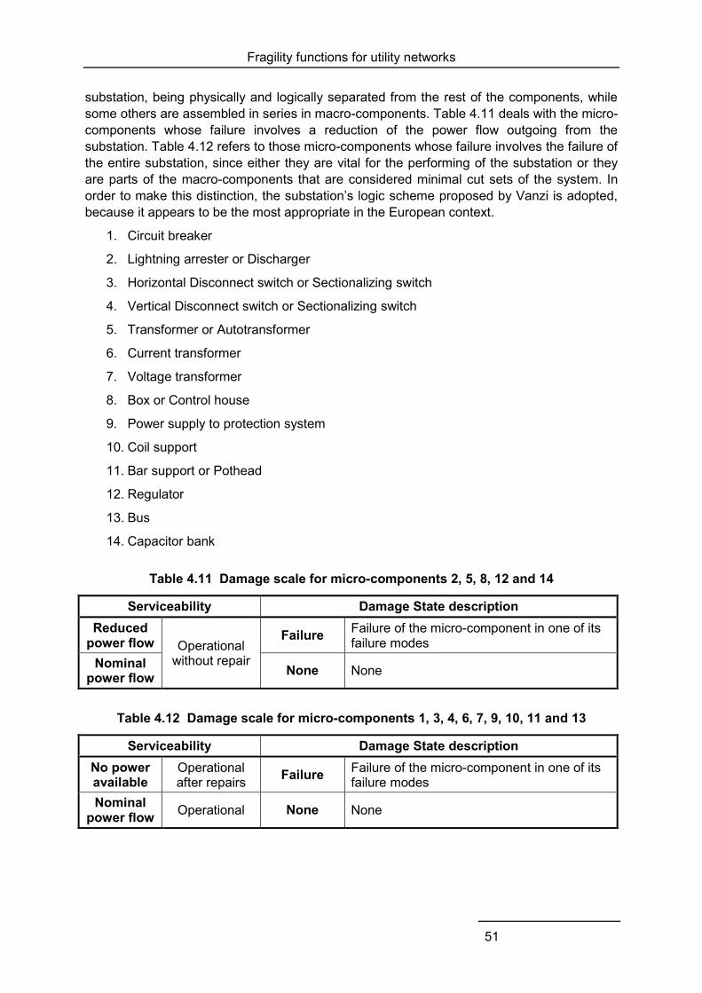
Fragility functions for utility networks
51
substation, being physically and logically separated from the rest of the components, while some others are assembled in series in macro-components. Table 4.11 deals with the micro-components whose failure involves a reduction of the power flow outgoing from the substation. Table 4.12 refers to those micro-components whose failure involves the failure of the entire substation, since either they are vital for the performing of the substation or they are parts of the macro-components that are considered minimal cut sets of the system. In order to make this distinction, the substation’s logic scheme proposed by Vanzi is adopted, because it appears to be the most appropriate in the European context.
1. Circuit breaker
2. Lightning arrester or Discharger
3. Horizontal Disconnect switch or Sectionalizing switch
4. Vertical Disconnect switch or Sectionalizing switch
5. Transformer or Autotransformer
6. Current transformer
7. Voltage transformer
8. Box or Control house
9. Power supply to protection system
10. Coil support
11. Bar support or Pothead
12. Regulator
13. Bus
14. Capacitor bank
Table 4.11 Damage scale for micro-components 2, 5, 8, 12 and 14
Serviceability Damage State description Reduced
power flow Operational without repair
Failure Failure of the micro-component in one of its failure modes
Nominal power flow None None
Table 4.12 Damage scale for micro-components 1, 3, 4, 6, 7, 9, 10, 11 and 13
Serviceability Damage State description No power available
Operational after repairs Failure Failure of the micro-component in one of its
failure modes Nominal
power flow Operational None None

Fragility functions for utility networks
52
4.1.4 Proposed fragility functions of electric power system components for use in SYNER-G systemic vulnerability analysis
In this section an appropriate fragility function is chosen from the available ones for the EPN macro- and micro-components that are of interest within SYNER-G (i.e. are employed within the systemic vulnerability analysis).The considered macro-components are those defined by Vanzi for which only the curves retrieved by Vanzi exist. Concerning the micro-components, the curves proposed by Vanzi have been obtained using data from shaking table tests on components installed in Italian substations. For this reason, compared with the other available curves, they appear to be the most appropriate in the European context and, hence, have been chosen for this study. The curves refer to components produced during the 80’s and 90’s, installed in substations of the Italian high voltage EPN (voltages ranging from 220 kV to 380 kV). For reference, the fragility functions proposed by HAZUS and UWG, for some micro-components are reported considering different voltage ranges and distinguishing between anchored and unanchored components. Macro-component 5 and micro-components 12, 13 and 14 have not been considered, since they are installed only in US substations.
Fragility functions of macro-components
Table 4.13 presents the fragility functions of the electric macro-components defined by Vanzi, listed here for reference.
1. Autotransformer line (autotransformer + dischargers + current transformers + circuit breakers + bearings)
2. Line without transformer (voltage transformer + coil support + sectionalizing switch + current transformer + circuit breaker + bearings)
3. Bars-connecting line (sectionalizing switch + current transformer + circuit breaker + bearings)
4. Bars (voltage transformer + bearings)
Fragility functions of micro-components
Table 4.14 presents the proposed fragility functions, adopted by Vanzi, of 11 electric micro-components. Components like line boxes, power supply to protection system and transformers are not standardized, hence they require ad hoc analyses. A standard reliability analysis has been carried out by Vanzi for these components, considering randomness in both the mechanical properties of concrete and steel and in the dynamic action. The probability of failure has then been computed via numerical integration from the probability distributions of the available and required ductilities.

Fragility functions for utility networks
53
Table 4.13 Proposed fragility functions of macro-components 1, 2, 3 and 4
Element at risk 4 electric macro-components Element Code EPN05 to 08
Reference Vanzi, I. 1996
Method Numerical, FORM/SORM methods
Function Lognormal, LN(λ, β)
Damage states Failure (Collapse)
IMT PGA (m/s2)
Background Fragilities of micro-components considered by the same author
Figures
Parameters (graphically retrieved from the curves)
Macro-component
25th perc. (m/s2)
Median (m/s2)
75th perc. (m/s2) λ (m/s2) β
Line without transformer 1.8 2.2 2.4 0.79 0.21
Bars-connecting line 2 2.4 2.6 0.88 0.19
Bars 1.2 1.5 2 0.41 0.38
Autotransformer line 1.5 1.8 2.3 0.59 0.32
Comments The considered macro-components are: (1) Line without transformer, (2) Bars-connecting line, (3) Bars, (4) Autotransformer line; The failures of interconnected vulnerable microelements are assumed as independent events
0 1 2 3 4 5 6 7 8 9 100
0.1
0.2
0.3
0.4
0.5
0.6
0.7
0.8
0.9
1
PGA (m/s2)
P [ D
S >
ds | P
GA
]
Macrocomponents
Line without transformer
Bars-connecting line
Bars
Autotransformer line

Fragility functions for utility networks
54
Table 4.14 Proposed fragility functions of 11 micro-components
Element at risk 11 electric micro-components Element Code EPN10 to EPN20
Reference Vanzi, I. 1996
Method Numerical Function Lognormal, LN(λ, β)
Damage states Failure (Collapse)
Intensity Measure Type, IMT PGA (m/s2) Background Cornell method
Figures
Parameters (extracted from a different reference)
Component λ (m/s2) β Component λ
(m/s2) β
Coil support 1.36 0.34 Discharger 2.27 0.32
Circuit breaker 1.66 0.33 Bar support 1.48 0.44
Current transformer 1.43 0.27 Autotransformer 3.16 0.29
Voltage transformer 1.79 0.27 Box 2.93 0.52
Horiz. sectionalizing switch 1.75 0.22 Power supply to
protection system 1.4 0.16
Vert. sectionalizing switch 1.69 0.34
Comments The retrieved fragility curves take into account the uncertainties about both the mechanical properties and the dynamic input
0 1 2 3 4 5 6 7 8 9 100
0.1
0.2
0.3
0.4
0.5
0.6
0.7
0.8
0.9
1
PGA (m/s2)
P [
DS
> d
s | P
GA
]
Microcomponents
Coil support
Circuit breaker
Current transformer
Voltage transformer
0 1 2 3 4 5 6 7 8 9 100
0.1
0.2
0.3
0.4
0.5
0.6
0.7
0.8
0.9
1
PGA (m/s2)
P [
DS
> d
s | P
GA
]
Microcomponents
Horizontal sectionalizing switch
Vertical sectionalizing switch
Discharger
Bar support
0 1 2 3 4 5 6 7 8 9 100
0.1
0.2
0.3
0.4
0.5
0.6
0.7
0.8
0.9
1
PGA (m/s2)
P [
DS
> d
s | P
GA
]
Microcomponents
Autotransformer
Box
Power supply
The considered micro-components are: (1) Coil support, (2) Circuit breaker, (3) Current transformer, (4) Voltage transformer, (5) Horizontal sectionalizing switch, (6) Vertical sectionalizing switch, (7) Discharger, (8) Bar support, (9) Autotransformer, (10) Box, (11) Power supply to protection system.
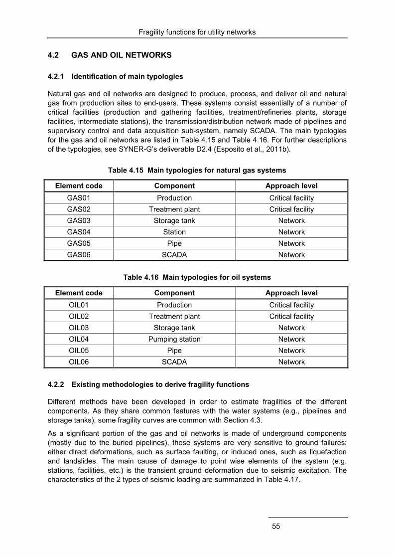
Fragility functions for utility networks
55
4.2 GAS AND OIL NETWORKS
4.2.1 Identification of main typologies
Natural gas and oil networks are designed to produce, process, and deliver oil and natural gas from production sites to end-users. These systems consist essentially of a number of critical facilities (production and gathering facilities, treatment/refineries plants, storage facilities, intermediate stations), the transmission/distribution network made of pipelines and supervisory control and data acquisition sub-system, namely SCADA. The main typologies for the gas and oil networks are listed in Table 4.15 and Table 4.16. For further descriptions of the typologies, see SYNER-G’s deliverable D2.4 (Esposito et al., 2011b).
Table 4.15 Main typologies for natural gas systems
Element code Component Approach level GAS01 Production Critical facility GAS02 Treatment plant Critical facility GAS03 Storage tank Network GAS04 Station Network GAS05 Pipe Network GAS06 SCADA Network
Table 4.16 Main typologies for oil systems
Element code Component Approach level OIL01 Production Critical facility OIL02 Treatment plant Critical facility OIL03 Storage tank Network OIL04 Pumping station Network OIL05 Pipe Network OIL06 SCADA Network
4.2.2 Existing methodologies to derive fragility functions
Different methods have been developed in order to estimate fragilities of the different components. As they share common features with the water systems (e.g., pipelines and storage tanks), some fragility curves are common with Section 4.3.
As a significant portion of the gas and oil networks is made of underground components (mostly due to the buried pipelines), these systems are very sensitive to ground failures: either direct deformations, such as surface faulting, or induced ones, such as liquefaction and landslides. The main cause of damage to point wise elements of the system (e.g. stations, facilities, etc.) is the transient ground deformation due to seismic excitation. The characteristics of the 2 types of seismic loading are summarized in Table 4.17.
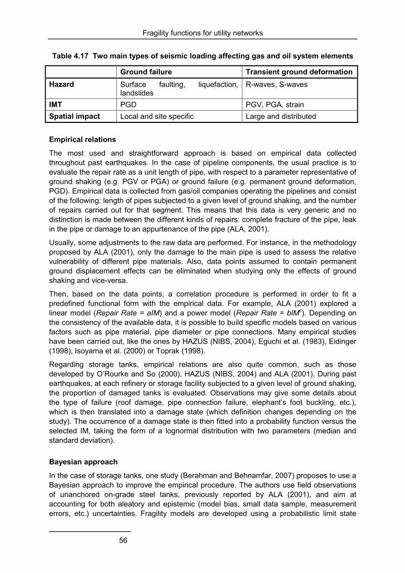
Fragility functions for utility networks
56
Table 4.17 Two main types of seismic loading affecting gas and oil system elements
Ground failure Transient ground deformation Hazard Surface faulting, liquefaction,
landslides R-waves, S-waves
IMT PGD PGV, PGA, strain Spatial impact Local and site specific Large and distributed
Empirical relations
The most used and straightforward approach is based on empirical data collected throughout past earthquakes. In the case of pipeline components, the usual practice is to evaluate the repair rate as a unit length of pipe, with respect to a parameter representative of ground shaking (e.g. PGV or PGA) or ground failure (e.g. permanent ground deformation, PGD). Empirical data is collected from gas/oil companies operating the pipelines and consist of the following: length of pipes subjected to a given level of ground shaking, and the number of repairs carried out for that segment. This means that this data is very generic and no distinction is made between the different kinds of repairs: complete fracture of the pipe, leak in the pipe or damage to an appurtenance of the pipe (ALA, 2001).
Usually, some adjustments to the raw data are performed. For instance, in the methodology proposed by ALA (2001), only the damage to the main pipe is used to assess the relative vulnerability of different pipe materials. Also, data points assumed to contain permanent ground displacement effects can be eliminated when studying only the effects of ground shaking and vice-versa.
Then, based on the data points, a correlation procedure is performed in order to fit a predefined functional form with the empirical data. For example, ALA (2001) explored a linear model (Repair Rate = aIM) and a power model (Repair Rate = bIMc). Depending on the consistency of the available data, it is possible to build specific models based on various factors such as pipe material, pipe diameter or pipe connections. Many empirical studies have been carried out, like the ones by HAZUS (NIBS, 2004), Eguchi et al. (1983), Eidinger (1998), Isoyama et al. (2000) or Toprak (1998).
Regarding storage tanks, empirical relations are also quite common, such as those developed by O’Rourke and So (2000), HAZUS (NIBS, 2004) and ALA (2001). During past earthquakes, at each refinery or storage facility subjected to a given level of ground shaking, the proportion of damaged tanks is evaluated. Observations may give some details about the type of failure (roof damage, pipe connection failure, elephant’s foot buckling, etc.), which is then translated into a damage state (which definition changes depending on the study). The occurrence of a damage state is then fitted into a probability function versus the selected IM, taking the form of a lognormal distribution with two parameters (median and standard deviation).
Bayesian approach
In the case of storage tanks, one study (Berahman and Behnamfar, 2007) proposes to use a Bayesian approach to improve the empirical procedure. The authors use field observations of unanchored on-grade steel tanks, previously reported by ALA (2001), and aim at accounting for both aleatory and epistemic (model bias, small data sample, measurement errors, etc.) uncertainties. Fragility models are developed using a probabilistic limit state
Fragility functions for utility networks
57
function and a reliability integral, solved with Monte-Carlo simulation. It was found that the fragility curves were less conservative than purely empirical models from ALA (2001) or NIBS (2004), suggesting a better tank performance than expected.
Analytical approach
In the case of buried pipelines, there are not many examples of analytical studies. Terzi et al. (2007) developed fragility curves for the case of segmented pipelines subjected to permanent ground deformation, using a Finite Element Model and accounting for pipe-soil interaction. The results were verified using the case of a polyvinyl chloride (PVC) pipe that suffered damage from the 2003 Lefkas earthquake.
Regarding storage tanks, a study by Iervolino et al. (2004) performs numeric analyses on dynamic models of unanchored steel tanks. Using a limit state function (e.g. axial stress, governing the failure by elephant’s foot buckling), the authors propose a decomposition of the random structural variable into those affecting the capacity (e.g. mechanical or material properties) and those affecting the demand (set of parameters defining the structure, shape, dimensions, etc.). A design of experiments is set up, with two axes (fluid level-over-radius ratio, and friction coefficient between the base-plate and the unanchored tank), and for each studied structure, a reliability analysis is performed in order to obtain a fragility curve. Then, through a second-order polynomial model, it is possible to obtain the response surface of the fragility parameters (median and standard deviation of the lognormal distribution).
Fault tree analysis (for support facilities)
In-line components or processing facilities such as gas compressor stations include many subcomponents, which make a quantitative vulnerability assessment quite difficult. In the configuration where support equipment (e.g. pumps, compressor, electric cabinets, etc.) are sheltered within a building, a solution is to treat these facilities as a common building. Thus, one can use the fragility curves for low-rise RC or masonry structures to assess the vulnerability of the compressor or pumping stations (see Chapter 3).
Another approach is to consider these facilities as systems and to aggregate the fragility of each component into a global systemic vulnerability. Such a work has been carried out in the SRMLIFE project (2003 – 2007) where a gas compressor station is decomposed into the following components:
o building;
o electrical / mechanical equipment;
o pump;
o commercial power;
o power backup.
Then, using the HAZUS (NIBS, 2004) fragility curves for these individual components and the curves from Kappos et al. (2006a) for the building, it is possible to compute the global fragility curve of the plant, based on the following fault-tree (Fig. 4.1).

Fragility functions for utility networks
58
Fig. 4.1 Decomposition of a compressor station into a fault-tree
The fault-tree decomposition follows a logic structure, with AND / OR operators that indicate how to aggregate the fragilities of two connected components. For two components A and B assembled in series (e.g. AND operator), like a pump and the building where it is stored into, the probability of failure of the system A-B is given by Pf(A-B) = Pf(A)Pf(B). On the other hand, when components A and B are mounted in parallel (e.g. OR operator), like commercial power connection and backup power, the probability of failure is expressed as Pf(AB) = 1 – [1 – Pf(A)] [1 – Pf(B)]. Using these basic rules, it is indeed possible to build up the global probability of failure of the compressor stations and to account for the fragility of both the building and the components inside.
4.2.3 Damage description
Pipeline components
As stated before, empirical relations for the fragility of pipelines are based on the recorded number of repairs during past earthquakes, and no distinction is really made between leaks and breaks of the pipes. As a result, all fragility relations for pipelines are given for a single “failure”, e.g. the repair rate (RR) per unit length of pipe. However, according to HAZUS (NIBS, 2004), the type of repair or damage depends on the type of hazard: a pipe damaged because of ground failure is likely to present a break (it is assumed 80% breaks and 20% leaks), whereas ground shaking may induce more leak-related damages (e.g. 20% breaks and 80% leaks).
Using a Poisson probability distribution and the repair rate RR, one can assess the probability of having n repairs in a pipe segment of length L:P(n) = e-RR L (RRL)n / n! Then, assuming that a pipe segment fails when it has at least one break/leak along its length, the probability of failure is given by Pf = 1 – P(N=0) = 1 –e-RRL. Finally, using the HAZUS assumption and considering the type of hazard, it is possible to assess the probability to have a pipe break or a pipe leak along the length of the segment.
Table 4.18 Proposed damage states for pipeline components
Damage state Damage description Serviceability DS1 no damage no break / leak Operational DS2 leakage at least one leak along the pipe length Reduction of the flow DS3 failure at least one break along the pipe length Disruption of the flow
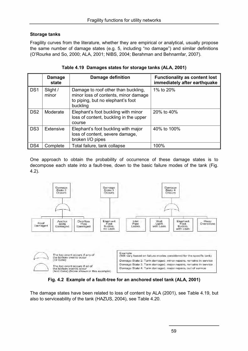
Fragility functions for utility networks
59
Storage tanks
Fragility curves from the literature, whether they are empirical or analytical, usually propose the same number of damage states (e.g. 5, including “no damage”) and similar definitions (O’Rourke and So, 2000; ALA, 2001; NIBS, 2004; Berahman and Behnamfar, 2007).
Table 4.19 Damages states for storage tanks (ALA, 2001)
Damage state
Damage definition Functionality as content lost immediately after earthquake
DS1 Slight / minor
Damage to roof other than buckling, minor loss of contents, minor damage to piping, but no elephant’s foot buckling
1% to 20%
DS2 Moderate Elephant’s foot buckling with minor loss of content, buckling in the upper course
20% to 40%
DS3 Extensive Elephant’s foot buckling with major loss of content, severe damage, broken I/O pipes
40% to 100%
DS4 Complete Total failure, tank collapse 100%
One approach to obtain the probability of occurrence of these damage states is to decompose each state into a fault-tree, down to the basic failure modes of the tank (Fig. 4.2).
Fig. 4.2 Example of a fault-tree for an anchored steel tank (ALA, 2001)
The damage states have been related to loss of content by ALA (2001), see Table 4.19, but also to serviceability of the tank (HAZUS, 2004), see Table 4.20.
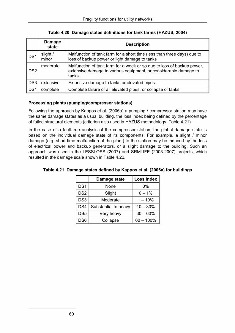
Fragility functions for utility networks
60
Table 4.20 Damage states definitions for tank farms (HAZUS, 2004)
Damage state Description
DS1 slight / minor
Malfunction of tank farm for a short time (less than three days) due to loss of backup power or light damage to tanks
DS2 moderate Malfunction of tank farm for a week or so due to loss of backup power,
extensive damage to various equipment, or considerable damage to tanks
DS3 extensive Extensive damage to tanks or elevated pipes DS4 complete Complete failure of all elevated pipes, or collapse of tanks
Processing plants (pumping/compressor stations)
Following the approach by Kappos et al. (2006a) a pumping / compressor station may have the same damage states as a usual building, the loss index being defined by the percentage of failed structural elements (criterion also used in HAZUS methodology, Table 4.21).
In the case of a fault-tree analysis of the compressor station, the global damage state is based on the individual damage state of its components. For example, a slight / minor damage (e.g. short-time malfunction of the plant) to the station may be induced by the loss of electrical power and backup generators, or a slight damage to the building. Such an approach was used in the LESSLOSS (2007) and SRMLIFE (2003-2007) projects, which resulted in the damage scale shown in Table 4.22.
Table 4.21 Damage states defined by Kappos et al. (2006a) for buildings
Damage state Loss index DS1 None 0% DS2 Slight 0 – 1% DS3 Moderate 1 – 10% DS4 Substantial to heavy 10 – 30% DS5 Very heavy 30 – 60% DS6 Collapse 60 – 100%
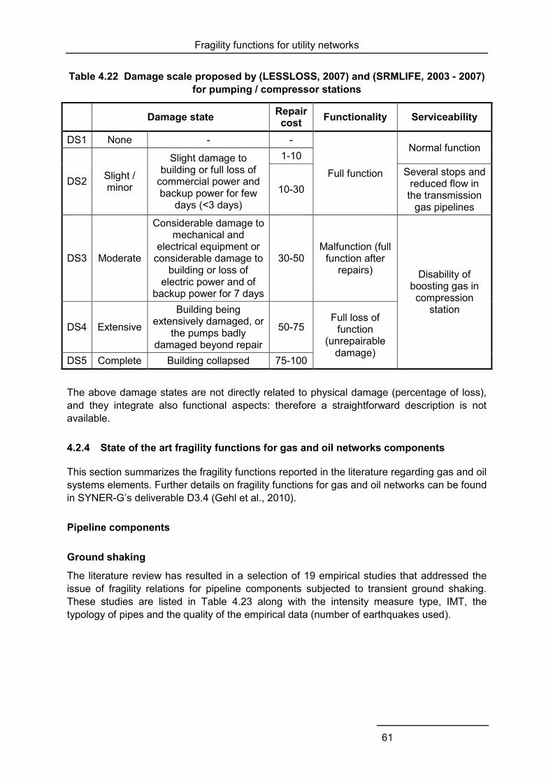
Fragility functions for utility networks
61
Table 4.22 Damage scale proposed by (LESSLOSS, 2007) and (SRMLIFE, 2003 - 2007) for pumping / compressor stations
Damage state Repair cost Functionality Serviceability
DS1 None - -
Full function
Normal function
DS2 Slight / minor
Slight damage to building or full loss of
commercial power and backup power for few
days (<3 days)
1-10
10-30
Several stops and reduced flow in the transmission
gas pipelines
DS3 Moderate
Considerable damage to mechanical and
electrical equipment or considerable damage to
building or loss of electric power and of
backup power for 7 days
30-50 Malfunction (full
function after repairs) Disability of
boosting gas in compression
station
DS4 Extensive
Building being extensively damaged, or
the pumps badly damaged beyond repair
50-75 Full loss of
function (unrepairable
damage) DS5 Complete Building collapsed 75-100
The above damage states are not directly related to physical damage (percentage of loss), and they integrate also functional aspects: therefore a straightforward description is not available.
4.2.4 State of the art fragility functions for gas and oil networks components
This section summarizes the fragility functions reported in the literature regarding gas and oil systems elements. Further details on fragility functions for gas and oil networks can be found in SYNER-G’s deliverable D3.4 (Gehl et al., 2010).
Pipeline components
Ground shaking
The literature review has resulted in a selection of 19 empirical studies that addressed the issue of fragility relations for pipeline components subjected to transient ground shaking. These studies are listed in Table 4.23 along with the intensity measure type, IMT, the typology of pipes and the quality of the empirical data (number of earthquakes used).
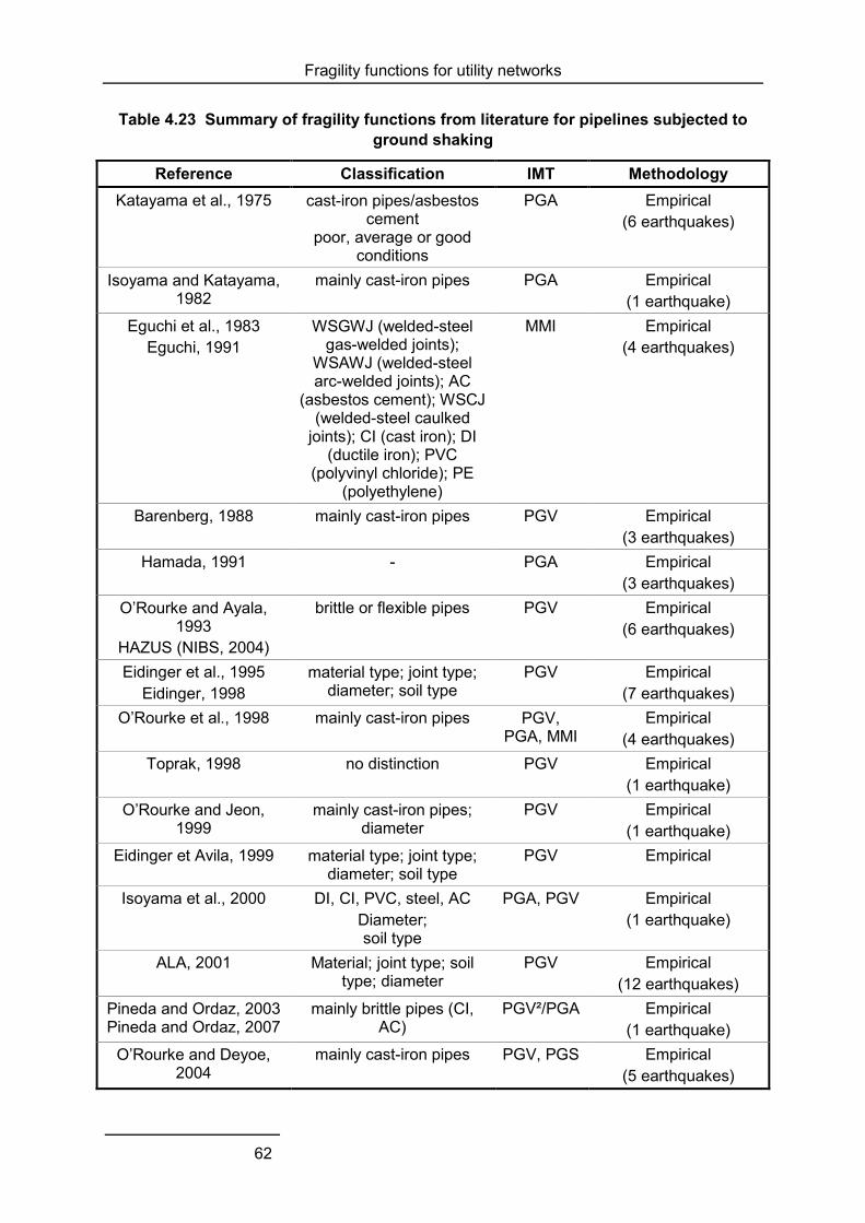
Fragility functions for utility networks
62
Table 4.23 Summary of fragility functions from literature for pipelines subjected to ground shaking
Reference Classification IMT Methodology Katayama et al., 1975 cast-iron pipes/asbestos
cement poor, average or good
conditions
PGA Empirical (6 earthquakes)
Isoyama and Katayama, 1982
mainly cast-iron pipes PGA Empirical (1 earthquake)
Eguchi et al., 1983 Eguchi, 1991
WSGWJ (welded-steel gas-welded joints);
WSAWJ (welded-steel arc-welded joints); AC
(asbestos cement); WSCJ (welded-steel caulked
joints); CI (cast iron); DI (ductile iron); PVC
(polyvinyl chloride); PE (polyethylene)
MMI Empirical (4 earthquakes)
Barenberg, 1988 mainly cast-iron pipes PGV Empirical (3 earthquakes)
Hamada, 1991 - PGA Empirical (3 earthquakes)
O’Rourke and Ayala, 1993
HAZUS (NIBS, 2004)
brittle or flexible pipes PGV Empirical (6 earthquakes)
Eidinger et al., 1995 Eidinger, 1998
material type; joint type; diameter; soil type
PGV Empirical (7 earthquakes)
O’Rourke et al., 1998 mainly cast-iron pipes PGV, PGA, MMI
Empirical (4 earthquakes)
Toprak, 1998 no distinction PGV Empirical (1 earthquake)
O’Rourke and Jeon, 1999
mainly cast-iron pipes; diameter
PGV Empirical (1 earthquake)
Eidinger et Avila, 1999 material type; joint type; diameter; soil type
PGV Empirical
Isoyama et al., 2000 DI, CI, PVC, steel, AC Diameter; soil type
PGA, PGV Empirical (1 earthquake)
ALA, 2001 Material; joint type; soil type; diameter
PGV Empirical (12 earthquakes)
Pineda and Ordaz, 2003 Pineda and Ordaz, 2007
mainly brittle pipes (CI, AC)
PGV²/PGA Empirical (1 earthquake)
O’Rourke and Deyoe, 2004
mainly cast-iron pipes PGV, PGS Empirical (5 earthquakes)
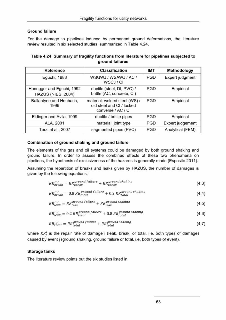
Fragility functions for utility networks
63
Ground failure
For the damage to pipelines induced by permanent ground deformations, the literature review resulted in six selected studies, summarized in Table 4.24.
Table 4.24 Summary of fragility functions from literature for pipelines subjected to ground failures
Reference Classification IMT Methodology Eguchi, 1983 WSGWJ / WSAWJ / AC /
WSCJ / CI PGD Expert judgment
Honegger and Eguchi, 1992 HAZUS (NIBS, 2004)
ductile (steel, DI, PVC) / brittle (AC, concrete, CI)
PGD Empirical
Ballantyne and Heubach, 1996
material: welded steel (WS) / old steel and CI / locked
converse / AC / CI
PGD Empirical
Eidinger and Avila, 1999 ductile / brittle pipes PGD Empirical ALA, 2001 material; joint type PGD Expert judgement
Terzi et al., 2007 segmented pipes (PVC) PGD Analytical (FEM)
Combination of ground shaking and ground failure
The elements of the gas and oil systems could be damaged by both ground shaking and ground failure. In order to assess the combined effects of these two phenomena on pipelines, the hypothesis of exclusiveness of the hazards is generally made (Esposito 2011).
Assuming the repartition of breaks and leaks given by HAZUS, the number of damages is given by the following equations:
(4.3)
(4.4)
(4.5)
(4.6)
(4.7)
where is the repair rate of damage i (leak, break, or total, i.e. both types of damage) caused by event j (ground shaking, ground failure or total, i.e. both types of event).
Storage tanks
The literature review points out the six studies listed in

Fragility functions for utility networks
64
Table 4.25, using the four different methods presented in Section 4.2.2.

Fragility functions for utility networks
65
Table 4.25 Summary of fragility functions from literature for storage tanks
Reference Classification IMT Methodology O’Rourke and So, 2000 Only On-grade steel tanks
ratio: tank’s height to diameter
relative amount of stored content
PGA Empirical (400 damaged tanks, 9
earthquakes) Log-normal distribution
ALA, 2001 Only On-grade steel tanks relative amount of stored
content anchorage of the tank to the
baseplate / unanchorage
PGA Empirical (400 damaged tanks, 9
earthquakes) Log-normal distribution
Berahman and Behnamfar, 2007
Only Unanchored on-grade steel tanks
PGA Bayesian approach (from empirical data)
Iervolino et al., 2004 Ratio fluid height/radius friction coefficient between the tank and the baseplate
PGA Analytical approach Log-normal distribution
NIBS, 2004 Anchored / unanchored components
PGA Fault tree analysis Log-normal distribution
Processing facilities
For processing facilities, only three studies have been selected from the literature review (Table 4.26).
Table 4.26 Summary of the fragility functions from literature for processing facilities
Reference Classification IMT Methodology LESSLOSS, 2007 Greek typology
Anchored subcomponents 1-3 floors
Low level / advanced seismic code
PGA Hybrid approach(fragility curves for buildings and Boolean logic tree for the
components) Lognormal distribution
HAZUS, 2004 Alexoudi, 2003
Anchored/ unanchored components
PGA Fault-tree analysis Lognormal distribution
4.2.5 Selection of appropriate fragility functions for European typologies
Pipeline components
The empirical relations found in the literature are suitable for most of the typologies of gas and oil pipelines in Europe (ductile pipes, mostly welded-steel and PVC). In view of the recommendations for intensity measures to be used for pipelines described in Deliverable 2.12(Weatherill et al., 2011), eight empirical relations constitute good candidates:
o for wave propagation (PGV): O’Rourke and Ayala (1993); Eidinger et al. (1998); Isoyama et al. (2001); ALA (2001);

Fragility functions for utility networks
66
o for permanent ground deformation (PGD): Eguchi (1983); Honegger and Eguchi (1992); Eidinger and Avila (1999); ALA (2001).
Among these different curves for wave propagation effect, the relation from ALA (2001) is the one applicable to the largest IMs range (Tromans, 2004). It has been built based on a global dataset (not only from US) and has been validated on the 1999 Düzce and 2003 Lefkas earthquakes. It has therefore been proposed as the one to be used in SYNER-G(Esposito et al., 2011a).
This curve shows some scatter and needs to be adapted with the correction factors (see Table B.3 in Appendix B), to fit the typology. Some materials used in Europe, for example HDPE in Italy, are not part of the present literature, but if they can be related to PVC pipelines as first approximation, it represents a conservative approach, because experience shows that HDPE pipelines tend to behave better.
For permanent ground failure, the relation from ALA (2001) is also based on the most complete database. Therefore, to be coherent with the curves for wave propagation, the curve from ALA (2001) with the correction factors listed in Table B.4 is proposed (see also the figures in Appendix B).
Storage tanks
Even though the studies by O’Rourke and So (2000) and ALA (2001) are the most thorough ones that account for different characteristics, the damage states they propose are related to physical damage to the tank body and do not consider the other components which may also alter the functionality of the tanks. Therefore, it is proposed here to use the curves developed with the HAZUS methodology (NIBS, 2004), with the characteristics presented in Table B.5 and the figures in Appendix B.
Processing facilities
The proposed curves are the existing ones reported in the literature. The fragility functions for the Greek-like typologies (low-rise masonry with anchored components) which could be used in SYNER-G are those developed in the SRMLIFE project. For the other types, the curves resulting from the HAZUS methodology (NIBS, 2004) are used for SYNER-G (Table B.7 and the figures in Appendix B). In cases where more information exists on the different fragilities of the components constituting the stations, fragility should be estimated based on fault tree-analysis (see Fig. 4.1).
4.2.6 Summary of the proposed fragility functions
The proposed fragility functions for the elements of gas and oil networks are outlined in Table 4.27. The parameters of these curves, together with their plots, are summarized in Appendix B.

Fragility functions for utility networks
67
Table 4.27 Summary of proposed fragility functions for elements of gas and oil systems
Element Methodology Classification IMT
Pipelines
ALA (2001) Empirical
Pipe material, joint type, soil type and pipe diameter PGV
ALA (2001) Expert judgment/
Empirical Pipe material, joint type PGD
Storage tanks HAZUS (2004) Anchored or unanchored components PGA Processing
facilities HAZUS (2004) Generic station, Anchored or unanchored components PGA
SRMLIFE (2007) Greek typology PGA
Fragility functions for utility networks
68
4.3 WATER AND WASTE-WATER NETWORKS
Water and waste water systems are generally prone to damage from earthquakes even under moderate levels of shaking. Furthermore, as experienced during past earthquakes, seismic damage to water system elements can cause extended direct and indirect economic losses, while environmental pollution is the main result of waste water network failures.
The main damages in both systems were observed in pipes; secondarily in pumping stations, tanks, lift stations and water/waste-water treatment plants. The pipeline damages can mainly be attributed to permanent ground deformation. Rigidity of the pipe body, connection type, age and corrosion are some of the factors that influence the seismic response of water and waste-water system elements.
4.3.1 Identification of main typologies
Typical water sources are springs, shallow or deep wells, rivers, natural lakes and impounding reservoirs. Wells are used in many cities both as primary and supplementary source of water. They include a pump to bring the water up to the surface, electromechanical equipment and a building to enclose the well and the equipment.
Water treatment plants are complex facilities that are generally composed of a number of connected physical and chemical unit processes whose roles are to improve the water quality. Common components include pre-sedimentation basins, aerators, detention tanks, flocculators, clarifiers, backwash tanks, conduit and channels, coal sand or sand filters, mixing tanks, settling tanks, clear wells, and chemical tanks.
A pumping station is a facility that boosts water pressure in both transmission and distribution systems. They typically comprise buildings, intake structures, pump and motor units, pipes, valves and associated electrical and control equipment. Main typology parameters include size, anchorage of subcomponents, equipment and backup power.
Pipes can be free-flow or pressure conduits, buried or elevated. In order to avoid contamination of treated water, potable water pipes are most of the time pressurized. Waste-water pipes, on the other hand, are most of the time free-flow conduits. Pipe typology depends on location (buried or elevated), material (type, strength), geometry (diameter, wall thickness), type of joints, continuous or segmented pipes, appurtenances and branches and corrosiveness (age and soil conditions).
Canals are free-flowing conduits, usually open to the atmosphere and usually at grade.
Storage tanks can be located at the start, along the length or at the end of a water transmission/distribution system. Their function may be to hold water for operational storage, provide surge relief volumes, provide detention times for disinfection, and other uses. Storage typology parameters may be the material (wood, steel or concrete), size, anchorage, position (at grade or elevated), type of roof, seismic design, foundation type, construction technique.
Waste-water treatment plants are complex facilities which include a number of buildings and underground or on-ground reinforced concrete tanks and basins. Common components include trickling filter, clarifiers, chlorine tanks, recirculation and waste-water pumping stations, chlorine storage and handling, tanks and pipelines. Concrete channels are
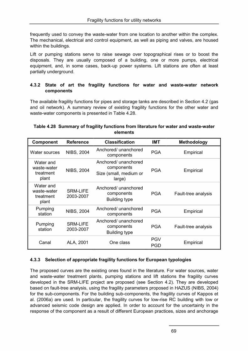
Fragility functions for utility networks
69
frequently used to convey the waste-water from one location to another within the complex. The mechanical, electrical and control equipment, as well as piping and valves, are housed within the buildings.
Lift or pumping stations serve to raise sewage over topographical rises or to boost the disposals. They are usually composed of a building, one or more pumps, electrical equipment, and, in some cases, back-up power systems. Lift stations are often at least partially underground.
4.3.2 State of art the fragility functions for water and waste-water network components
The available fragility functions for pipes and storage tanks are described in Section 4.2 (gas and oil network). A summary review of existing fragility functions for the other water and waste-water components is presented in Table 4.28.
Table 4.28 Summary of fragility functions from literature for water and waste-water elements
Component Reference Classification IMT Methodology
Water sources NIBS, 2004 Anchored/ unanchored components PGA Empirical
Water and waste-water
treatment plant
NIBS, 2004
Anchored/ unanchored components
Size (small, medium or large)
PGA Empirical
Water and waste-water
treatment plant
SRM-LIFE 2003-2007
Anchored/ unanchored components Building type
PGA Fault-tree analysis
Pumping station NIBS, 2004 Anchored/ unanchored
components PGA Empirical
Pumping station
SRM-LIFE 2003-2007
Anchored/ unanchored components Building type
PGA Fault-tree analysis
Canal ALA, 2001 One class PGV PGD Empirical
4.3.3 Selection of appropriate fragility functions for European typologies
The proposed curves are the existing ones found in the literature. For water sources, water and waste-water treatment plants, pumping stations and lift stations the fragility curves developed in the SRM-LIFE project are proposed (see Section 4.2). They are developed based on fault-tree analysis, using the fragility parameters proposed in HAZUS (NIBS, 2004) for the sub-components. For the building sub-components, the fragility curves of Kappos et al. (2006a) are used. In particular, the fragility curves for low-rise RC building with low or advanced seismic code design are applied. In order to account for the uncertainty in the response of the component as a result of different European practices, sizes and anchorage
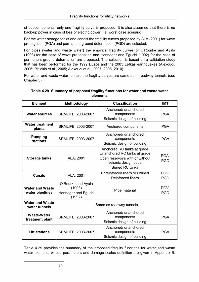
Fragility functions for utility networks
70
of subcomponents, only one fragility curve is proposed. It is also assumed that there is no back-up power in case of loss of electric power (i.e. worst case scenario).
For the water storage tanks and canals the fragility curves proposed by ALA (2001) for wave propagation (PGA) and permanent ground deformation (PGD) are selected.
For pipes (water and waste water) the empirical fragility curves of O’Rourke and Ayala (1993) for the case of wave propagation and Honneger and Eguchi (1992) for the case of permanent ground deformation are proposed. The selection is based on a validation study that has been performed for the 1999 Düzce and the 2003 Lefkas earthquakes (Alexoudi, 2005; Pitilakis et al., 2005; Alexoudi et al., 2007, 2008, 2010).
For water and waste water tunnels the fragility curves are same as in roadway tunnels (see Chapter 5).
Table 4.29 Summary of proposed fragility functions for water and waste water elements
Element Methodology Classification IMT
Water sources SRMLIFE, 2003-2007 Anchored/ unanchored
components Seismic design of building
PGA
Water treatment plants SRMLIFE, 2003-2007 Anchored components PGA
Pumping stations SRMLIFE, 2003-2007
Anchored/ unanchored components
Seismic design of building PGA
Storage tanks ALA, 2001
Anchored RC tanks at grade Unanchored RC tanks at grade Open reservoirs with or without
seismic design code Buried RC tanks
PGA, PGD
Canals ALA, 2001 Unreinforced liners or unlined Reinforced liners
PGV, PGD
Water and Waste water pipelines
O’Rourke and Ayala (1993)
Honneger and Eguchi (1992)
Pipe material PGV, PGD
Water and Waste water tunnels Same as roadway tunnels
Waste-Water treatment plant SRMLIFE, 2003-2007
Anchored/ unanchored components
Seismic design of building PGA
Lift stations SRMLIFE, 2003-2007 Anchored/ unanchored
components Seismic design of building
PGA
Table 4.29 provides the summary of the proposed fragility functions for water and waste water elements whose parameters and damage scales definition are given in Appendix B.

Fragility functions for utility networks
71
Damage scale definitions are also related to the functionality of the components, their serviceability in terms of usage (nominal use, reduced use or not usable) and repair capability (usable without repairs, after repairs or not repairable). Alternatively, a damage factor or replacement cost (usually between 0 and 1 or 100%) can be provided.

Fragility functions for transportation infrastructures
73
5 Fragility functions for transportation infrastructures
Transportation systems include roadway, railway and subway networks, port and airport systems and infrastructures. Each system is actually a complex network of various components like bridges, roads, tunnels, embankments, retaining walls, slopes in case of roadway system or wharfs, cranes, buildings, utility systems, and tanks in case of harbour. Experience from past earthquakes reveals that these elements are quite vulnerable, while their damage could be greatly disruptive due to the lack of redundancy, the lengthy repair time or the rerouting difficulties. For example, the disruption to the road network can strongly affect the emergency efforts immediately after the earthquake or the rebuild and other business activities in the following period. A typical paradigm is the port of Kobe after the strong Great Hansin earthquake (M7.1, 1995) that has lost almost 50% of its annual income, despite the enormous retrofitting works.
The complexity of elements at risk, their variability from one place and one country to another, and until recently, the lack of well-documented damage and loss data from strong earthquakes and the spatial variability of ground motion, make the vulnerability assessment of each particular component and of the network as a whole, a quite complicated problem. Addition of the spatial extension of transportation networks, the interactions with other systems and the inherent uncertainties in seismic hazard and vulnerability estimates, makes the risk assessment of transportation networks indeed a complex and challenging issue.
In the following sections, a brief review of available fragility curves and their evaluation methods are presented. The main typological features, damage states and parameters of the proposed fragility functions are given for roadway bridges, roadway and railway elements, and harbour infrastructures. The parameters, damage states and plots of the fragility curves are given in appendix C for each element. For further details, the reader is referred to SYNER-G Deliverables 3.6, 3.7, 3.8 and 3.9.
5.1 ROADWAY AND RAILWAY BRIDGES
Work Package 3 concerned the identification of fragility functions for elements and systems and, specifically, Task 3.6 aimed at identifying the main typologies of bridges in Europe and review of existing fragility functions, to compare these functions amongst themselves and eventually compare them with new functions developed in SYNER-G. The study has mainly comprised of a literature review which has led to a collection of existing fragility functions (as reported in Appendix A of Deliverable 3.6) and the identification of categories for grouping bridges (a taxonomy) and for harmonising different intensity measures and limit states. The main output of the study was a set of fragility functions (with associated uncertainties) for the main bridges typologies.
The first step involved the identification and the storage of the existing fragility function sets with a focus on European practice. An effort in collecting the existing studies concerning fragility functions has been carried out, together with an effort in constructing a tool able to store and process the fragility function sets that were collected. The SYNER-G ‘Fragility
Fragility functions for transportation infrastructures
74
Function Manager’ tool introduced in Chapter 1 is able to store, visualize and manage a large number of fragility functions sets, for both buildings and bridges.
Within this project, a different approach for categorizing and classifying bridges and thus a new taxonomy has been proposed in order to homogenize the existing model bridge types. Subsequently, it has been possible to develop the next step of this task, which is the comparison amongst existing fragility functions. Two different modules have thus been developed in the tool, namely, the Harmonize module and the Compare module. The former function allows one to harmonize the curves using a target intensity measure type (which has been selected as PGA herein) and a number of limit states of reference (which have been selected as yielding and collapse herein). After the harmonisation, the Compare function can be used to plot and compare the different curves, and to calculate the mean and dispersion of the parameters of the curves. It should be noted that the Filter function in the tool allows the user to first select the bridge types that are feasibly comparable, in terms of fragility. In addition, a new approach has been implemented for the creation of analytical fragility functions for bridges in Europe (see Section 5.1.2).
Section 5.1.1 of this chapter describes briefly the methodologies, the intensity measure types and the limit states that have been found in the reviewed fragility studies. Section 5.1.2 explains the methodology developed within this project for deriving fragility functions for bridges. Section 5.1.3 presents an overview of some existing taxonomies used to describe different classes of bridges, and the taxonomy proposed within this project to identify European bridges. Sections 5.1.4 and 5.1.5 relate specifically to the SYNER-G Fragility Function Manager. In particular, the procedures to harmonize and compare fragility curves for a given bridge typology are discussed.
5.1.1 Existing fragility functions for European bridges
The vulnerable conditions of a bridge can be described using fragility functions. A large number of fragility functions have been collected and stored in the SYNER-G’s Fragility Function Manager tool (see Chapter 1 and the tutorial in Appendix B of Deliverable 3.6). For each fragility study that has been considered, a review form has been filled in with a brief summary of the functions. The form is comprised of different fields:
o Reference: reference papers, documents, deliverables;
o Region of applicability: this region represents the reference place for which bridges have been analysed and fragility functions have been developed;
o Element at risk: list of the elements at risk considered by the fragility functions (i.e., buildings, bridges, lifelines, infrastructures, etc.);
o Typology of the element at risk considered: based on the original description provided in the references (i.e. RC – multi-span – with seismic design);
o SYNER-G Taxonomy: the description of the element at risk using the taxonomy proposed within this project (detailed description in SYNER-G Reference Report 2);
o Sample Data: description of the data (i.e., structures, accelerograms, etc.) that are considered in the analyses to estimate the fragility functions;
o Methodology: methodology used to estimate the fragility functions (empirical, analytical – nonlinear static, analytical – nonlinear dynamic, etc.);
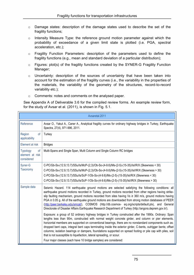
Fragility functions for transportation infrastructures
75
o Damage states: description of the damage states used to describe the set of the fragility functions;
o Intensity Measure Type: the reference ground motion parameter against which the probability of exceedance of a given limit state is plotted (i.e. PGA, spectral acceleration, etc.);
o Fragility Function Parameters: description of the parameters used to define the fragility functions (e.g., mean and standard deviation of a particular distribution);
o Figures: plot(s) of the fragility functions created by the SYNER-G Fragility Function Manager;
o Uncertainty: description of the sources of uncertainty that have been taken into account for the estimation of the fragility curves (i.e., the variability in the properties of the materials, the variability of the geometry of the structures, record-to-record variability etc.);
o Comments: notes and comments on the analysed paper.
See Appendix A of Deliverable 3.6 for the compiled review forms. An example review form, for the study of Avsar et al. (2011), is shown in Fig. 5.1.
Avsaretal.2011
Reference Avsar O., Yakut A., Caner A., Analytical fragility curves for ordinary highway bridges in Turkey, Earthquake
Spectra, 27(4), 971-996, 2011.
Region of
applicability
Turkey
Element at risk Bridges
Typology of
element at risk
considered
Multi-Spans and Single Span, Multi Column and Single Column RC bridges
Syner-G
Taxonomy
C-PC/Gb-Ss-(12.9,13.7)/SSu/Is/McP-(2,3)/Ob-So-(4-9.6)/Ms-(2-5)-(15-35)/IsI/R/X (Skewness < 30)
C-PC/Gb-Ss-(12.9,13.7)/SSu/Is/McP-(2,3)/Ob-So-(4-9.6)/Ms-(2-5)-(15-35)/IsI/IR/X (Skewness > 30)
C-PC/Gb-Ss-(12.9,13.7)/SSu/Is/ScP-1/Ob-So-(4-9.6)/Ms-(2-5)-(15-35)/IsI/R/X (Skewness < 30)
C-PC/Gb-Ss-(12.9,13.7)/SSu/Is/ScP-1/Ob-So-(4-9.6)/Ms-(2-5)-(15-35)/IsI/IR/X (Skewness > 30)
Sample data Seismic Hazard. 114 earthquake ground motions are selected satisfying the following conditions: all
earthquake ground motions recorded in Turkey, ground motions recorded from other regions having strike-
slip faulting mechanism, ground motions recorded from sites having Vs ≥ 360 m/s, ground motions having
PGA ≥ 0.05 g. All of the earthquake ground motions are downloaded from strong motion databases of PEER
(http://peer.berkeley.edu/smcat/), COSMOS (http://db.cosmos- eq.org/scripts/default.plx), and General
Directorate of Disaster Affairs Earthquake Research Department of Turkey (http://angora.deprem.gov.tr/).
Exposure: a group of 52 ordinary highway bridges in Turkey constructed after the 1990s. Ordinary: Span
lengths less than 90m, constructed with normal weight concrete girder, and column or pier elements,
horizontal members are supported on conventional bearings, there are no nonstandard components such as;
dropped bent caps, integral bent caps terminating inside the exterior girder, C-bents, outrigger bents; offset
columns; isolation bearings or dampers, foundations supported on spread footing or pile cap with piles, soil
that is not susceptible to liquefaction, lateral spreading, or scour.
Four major classes (each have 10 bridge samples) are considered:

Fragility functions for transportation infrastructures
76
Abbreviation Bridge Classes
MS_MC_SL30 Multi Span – Multi Column – Skewness Less than 30°
MS_MC_SG30 Multi Span – Multi Column – Skewness Greater than 30°
MS_SC_SL30 Multi Span – Single Column – Skewness Less than 30°
MS_SC_SG30 Multi Span – Single Column – Skewness Greater than 30°
Methodology Analytical – Nonlinear Dynamic
Damage States Three damage states:
Serviceability: LS1
Damage Control: LS2
Collapse Prevention: LS3
Intensity
Measure Type
PGA, PGV, ASI
Fragility
Function
Parameters
Lognormal Distribution
IMT = PGA [g]
LS1 LS2 LS3
Mean StDev Mean StDev Mean StDev
MS_MC_SL30 0.127 0.053 0.721 0.206 0.913 0.296
MS_MC_SG30 0.107 0.057 0.620 0.224 0.813 0.320
MS_SC_SL30 0.122 0.058 0.625 0.260 0.831 0.423
MS_SC_SG30 0.109 0.048 0.514 0.191 0.664 0.277
IMT = PGV [cm/s]
LS1 LS2 LS3
Mean StDev Mean Mean StDev Mean
MS_MC_SL30 12.458 5.960 70.325 43.842 88.044 61.219
MS_MC_SG30 11.220 2.673 56.574 32.358 73.980 45.837
MS_SC_SL30 11.800 4.311 50.004 25.810 65.951 37.478
MS_SC_SG30 10.870 4.357 36.473 17.026 54.988 31.655
IMT = ASI [g*s]
LS1 LS2 LS3
Mean StDev Mean Mean StDev Mean
MS_MC_SL30 0.131 0.055 0.617 0.183 0.727 0.229
MS_MC_SG30 0.146 0.055 0.516 0.143 0.653 0.207
MS_SC_SL30 0.143 0.057 0.472 0.191 0.635 0.242
MS_SC_SG30 0.131 0.047 0.376 0.157 0.547 0.219

Fragility functions for transportation infrastructures
77
Figures
MS-MC-SL30-PGA MS-MC-SG30-PGA
MS-SC-SL30-PGA MS-SC-SG30-PGA
MS-MC-SL30-PGV MS-MC-SG30-PGV
MS-SC-SL30-PGV MS-SC-SG30-PGV
LS1 LS2 LS3
PGA [g]10.90.80.70.60.50.40.30.20.10
Prob
abilit
y of
exc
eeda
nce
1
0.8
0.6
0.4
0.2
0
LS1 LS2 LS3
PGA [g]10.90.80.70.60.50.40.30.20.10
Prob
abilit
y of
exc
eeda
nce
1
0.8
0.6
0.4
0.2
0
LS1 LS2 LS3
PGA [g]10.90.80.70.60.50.40.30.20.10
Pro
babi
lity
of e
xcee
danc
e
1
0.8
0.6
0.4
0.2
0
LS1 LS2 LS3
PGA [g]10.90.80.70.60.50.40.30.20.10
Pro
babi
lity
of e
xcee
danc
e
1
0.8
0.6
0.4
0.2
0
LS1 LS2 LS3
PGV [cm/s]1009080706050403020100
Pro
babi
lity
of e
xcee
danc
e
1
0.8
0.6
0.4
0.2
0
LS1 LS2 LS3
PGV [cm/s]1009080706050403020100
Prob
abilit
y of
exc
eeda
nce
1
0.8
0.6
0.4
0.2
0
LS1 LS2 LS3
PGV [cm/s]1009080706050403020100
Prob
abilit
y of
exc
eeda
nce
1
0.8
0.6
0.4
0.2
0
LS1 LS2 LS3
PGV [cm/s]1009080706050403020100
Prob
abilit
y of
exc
eeda
nce
1
0.8
0.6
0.4
0.2
0
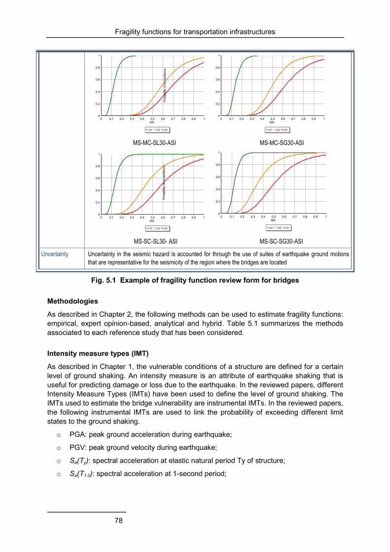
Fragility functions for transportation infrastructures
78
MS-MC-SL30-ASI MS-MC-SG30-ASI
MS-SC-SL30- ASI MS-SC-SG30-ASI
Uncertainty Uncertainty in the seismic hazard is accounted for through the use of suites of earthquake ground motions
that are representative for the seismicity of the region where the bridges are located
Fig. 5.1 Example of fragility function review form for bridges
Methodologies
As described in Chapter 2, the following methods can be used to estimate fragility functions: empirical, expert opinion-based, analytical and hybrid. Table 5.1 summarizes the methods associated to each reference study that has been considered.
Intensity measure types (IMT)
As described in Chapter 1, the vulnerable conditions of a structure are defined for a certain level of ground shaking. An intensity measure is an attribute of earthquake shaking that is useful for predicting damage or loss due to the earthquake. In the reviewed papers, different Intensity Measure Types (IMTs) have been used to define the level of ground shaking. The IMTs used to estimate the bridge vulnerability are instrumental IMTs. In the reviewed papers, the following instrumental IMTs are used to link the probability of exceeding different limit states to the ground shaking.
o PGA: peak ground acceleration during earthquake;
o PGV: peak ground velocity during earthquake;
o Sa(Ty): spectral acceleration at elastic natural period Ty of structure;
o Sa(T1.0): spectral acceleration at 1-second period;
LS1 LS2 LS3
ASI 10.90.80.70.60.50.40.30.20.10
Pro
babi
lity
of e
xcee
danc
e
1
0.8
0.6
0.4
0.2
0
LS1 LS2 LS3
ASI 10.90.80.70.60.50.40.30.20.10
Pro
babi
lity
of e
xcee
danc
e
1
0.8
0.6
0.4
0.2
0
LS1 LS2 LS3
ASI 10.90.80.70.60.50.40.30.20.10
Pro
babi
lity
of e
xcee
danc
e
1
0.8
0.6
0.4
0.2
0
LS1 LS2 LS3
ASI 10.90.80.70.60.50.40.30.20.10
Prob
abilit
y of
exc
eeda
nce
1
0.8
0.6
0.4
0.2
0

Fragility functions for transportation infrastructures
79
Table 5.1 List of references considered and corresponding methods
Method Reference Empirical Basoz et al., 1999
Elnashai et al., 2004 Karim and Yamazaki, 2001 Shinozuka et al., 2000a Shinozuka, 2003
Analytical – Nonlinear Static Azevedo et al., 2010 Cardone et al., 2011 Fardis et al., 2011 Karakostas et al., 2006 Mander, 1999 Monti and Nisticò, 2002 Moschonas et al., 2009 Shinozuka et al., 2000b
Analytical – Nonlinear Dynamic
Avsar et al., 2011 Banerjee and Shinozuka, 2008 Choi et al., 2004 Elnashai et al., 2004 Franchin et al., 2008 Jeong and Elnashai, 2007 Kappos et al., 2006b Karim and Yamazaki, 2001 Karim and Yamazaki, 2003 Kibboua et al., 2011 Lupoi et al., 2005 Nielson and Des Roches, 2007 Nielson, 2005 Padgett and Des Roches, 2009 Saxena et al., 2000 Shinozuka et al., 2000a Shirazian et al., 2011 Yi et al., 2007
o Sa(Tgm): spectral acceleration at geometric mean of fundamental periods of longitudinal and transverse directions (Tgm);
o ASI: acceleration spectrum intensity, given by the area under the elastic response spectrum (5% damped) within the boundary periods Ti and Tf, defined as the initial and final periods to be used in the calculation of ASI;
o SI: spectrum intensity;
o Return Period: the mean interval of time between ground-motion of a certain intensity.
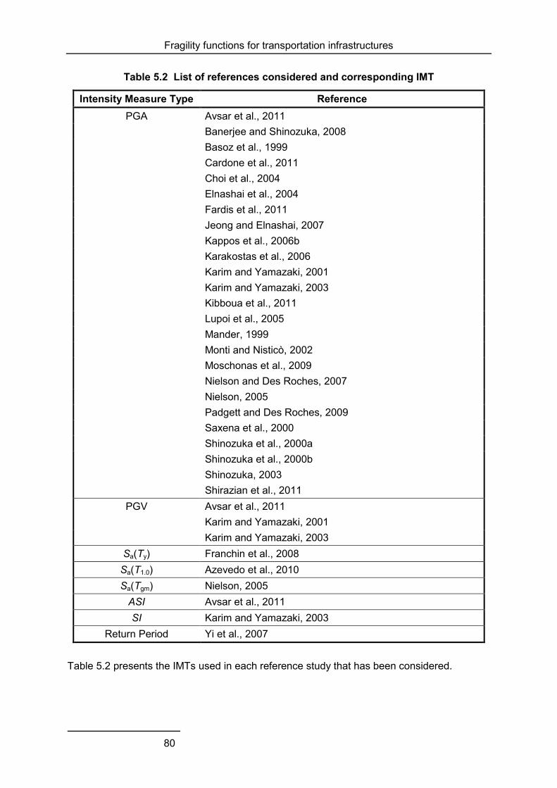
Fragility functions for transportation infrastructures
80
Table 5.2 List of references considered and corresponding IMT
Intensity Measure Type Reference PGA Avsar et al., 2011
Banerjee and Shinozuka, 2008 Basoz et al., 1999 Cardone et al., 2011 Choi et al., 2004 Elnashai et al., 2004 Fardis et al., 2011 Jeong and Elnashai, 2007 Kappos et al., 2006b Karakostas et al., 2006 Karim and Yamazaki, 2001 Karim and Yamazaki, 2003 Kibboua et al., 2011 Lupoi et al., 2005 Mander, 1999 Monti and Nisticò, 2002 Moschonas et al., 2009 Nielson and Des Roches, 2007 Nielson, 2005 Padgett and Des Roches, 2009 Saxena et al., 2000 Shinozuka et al., 2000a Shinozuka et al., 2000b Shinozuka, 2003 Shirazian et al., 2011
PGV Avsar et al., 2011 Karim and Yamazaki, 2001 Karim and Yamazaki, 2003
Sa(Ty) Franchin et al., 2008 Sa(T1.0) Azevedo et al., 2010 Sa(Tgm) Nielson, 2005
ASI Avsar et al., 2011 SI Karim and Yamazaki, 2003
Return Period Yi et al., 2007
Table 5.2 presents the IMTs used in each reference study that has been considered.
Fragility functions for transportation infrastructures
81
Limit states
As mentioned in Section 1.1, the performance levels of a bridge can be defined through damage thresholds called limit states. A limit state defines the threshold between different damage conditions, whereas the damage states define the damage conditions themselves (see Fig. 3.1). For instance, if the performance of a bridge is described by two limit states (Limit State 1 and Limit State 2), there will be three damage states (Damage State 1, Damage State 2 and Damage State 3).
5.1.2 Development of new fragility functions
Fragility curves were produced for prototype regular bridges with continuous deck as a function of the deck-pier connection (monolithic or through elastomeric bearings), the transverse translation at the abutments (free or constrained), the bridge length L, the type of pier cross-section (hollow rectangular, wall-type rectangular, circular), the number of columns per pier, the pier height h and the level of seismic design (design to EC2 (CEN 2005b) alone, or to EC8 (CEN 2005c) with a design PGA on top of the rock of 0.25g).
For railway bridges the deck is taken as transversely constrained at the abutments; for road bridges it is transversely free. The pier dimensions are chosen so that 2nd-order effects may be neglected, according to EC2 (CEN 2004a). Their reinforcement is dimensioned for the ULS in bending with axial load and in shear for the persistent-and-transient and the seismic design situations. Bearings are dimensioned per EN 1337 (CEN 2005e), for the same design situations. Seismic analysis is performed for the EC8 design spectrum and different q-factors for bridges with limited ductile or ductile behaviour. EC8’s “rigid deck model” is used in the longitudinal direction of all bridges and in the transverse one of those with free transverse translation at the abutments. Modal response spectrum analysis is applied in the transverse direction of bridges with constrained transverse translation at the abutments.
The following are the bases of the derivations. Two damage states are considered: yielding and ultimate. PGA is selected as the intensity measure type. Damage measures for the piers are the peak chord rotation and the peak shear force. The damage measure for bearings is the relative displacement between the deck and the pier top that may cause rollover and the shear deformation. The operational limits for the deck of railway bridges (CEN 2005a) are also checked.
Inelastic or elastic seismic displacement and deformation demands are estimated with the “equal displacement rule”. The only difference with the analysis for the design is that the unreduced 5%-damped elastic spectrum is used. Following the sequence of plastic hinge formation at pier ends, the shear forces are determined from the mean values of moment resistances. The seismic analyses give the median value of the damage measure of interest as a function of PGA. The (conditional on PGA) probability of exceedance of each damage state is computed from the probability distributions of the damage measure demands (conditional on PGA) and of the corresponding capacities. The expected values of the capacity of piers are established from the expressions in Biskinis and Fardis (2010a, 2010b) and Biskinis at al. (2004) that also give their cv, reflecting the uncertainty in the models. The cv-values for the pier deformation demands for given excitation spectrum are based on Bardakis and Fardis (2011); those for the bearings are taken from the literature and the tests performed at the UPAT Structures Lab.
Fragility curves are constructed for each pier or bearing for the seismic action separately in the two directions of the bridge. The fragility curve of a component at a given damage state
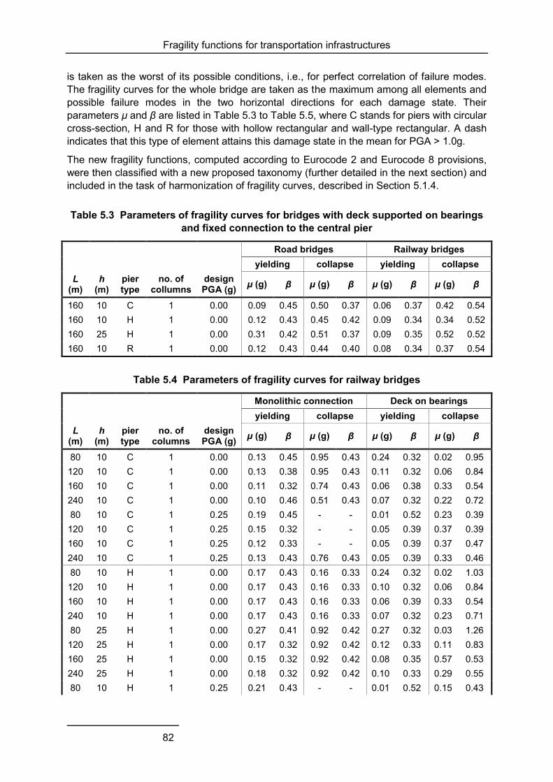
Fragility functions for transportation infrastructures
82
is taken as the worst of its possible conditions, i.e., for perfect correlation of failure modes. The fragility curves for the whole bridge are taken as the maximum among all elements and possible failure modes in the two horizontal directions for each damage state. Their parameters μ and β are listed in Table 5.3 to Table 5.5, where C stands for piers with circular cross-section, H and R for those with hollow rectangular and wall-type rectangular. A dash indicates that this type of element attains this damage state in the mean for PGA > 1.0g.
The new fragility functions, computed according to Eurocode 2 and Eurocode 8 provisions, were then classified with a new proposed taxonomy (further detailed in the next section) and included in the task of harmonization of fragility curves, described in Section 5.1.4.
Table 5.3 Parameters of fragility curves for bridges with deck supported on bearings and fixed connection to the central pier
Road bridges Railway bridges yielding collapse yielding collapse
L (m)
h (m)
pier type
no. of collumns
design PGA (g) μ (g) β μ (g) β μ (g) β μ (g) β
160 10 C 1 0.00 0.09 0.45 0.50 0.37 0.06 0.37 0.42 0.54 160 10 H 1 0.00 0.12 0.43 0.45 0.42 0.09 0.34 0.34 0.52 160 25 H 1 0.00 0.31 0.42 0.51 0.37 0.09 0.35 0.52 0.52 160 10 R 1 0.00 0.12 0.43 0.44 0.40 0.08 0.34 0.37 0.54
Table 5.4 Parameters of fragility curves for railway bridges
Monolithic connection Deck on bearings yielding collapse yielding collapse
L (m)
h (m)
pier type
no. of columns
design PGA (g) μ (g) β μ (g) β μ (g) β μ (g) β
80 10 C 1 0.00 0.13 0.45 0.95 0.43 0.24 0.32 0.02 0.95 120 10 C 1 0.00 0.13 0.38 0.95 0.43 0.11 0.32 0.06 0.84 160 10 C 1 0.00 0.11 0.32 0.74 0.43 0.06 0.38 0.33 0.54 240 10 C 1 0.00 0.10 0.46 0.51 0.43 0.07 0.32 0.22 0.72 80 10 C 1 0.25 0.19 0.45 - - 0.01 0.52 0.23 0.39 120 10 C 1 0.25 0.15 0.32 - - 0.05 0.39 0.37 0.39 160 10 C 1 0.25 0.12 0.33 - - 0.05 0.39 0.37 0.47 240 10 C 1 0.25 0.13 0.43 0.76 0.43 0.05 0.39 0.33 0.46 80 10 H 1 0.00 0.17 0.43 0.16 0.33 0.24 0.32 0.02 1.03 120 10 H 1 0.00 0.17 0.43 0.16 0.33 0.10 0.32 0.06 0.84 160 10 H 1 0.00 0.17 0.43 0.16 0.33 0.06 0.39 0.33 0.54 240 10 H 1 0.00 0.17 0.43 0.16 0.33 0.07 0.32 0.23 0.71 80 25 H 1 0.00 0.27 0.41 0.92 0.42 0.27 0.32 0.03 1.26 120 25 H 1 0.00 0.17 0.32 0.92 0.42 0.12 0.33 0.11 0.83 160 25 H 1 0.00 0.15 0.32 0.92 0.42 0.08 0.35 0.57 0.53 240 25 H 1 0.00 0.18 0.32 0.92 0.42 0.10 0.33 0.29 0.55 80 10 H 1 0.25 0.21 0.43 - - 0.01 0.52 0.15 0.43

Fragility functions for transportation infrastructures
83
Monolithic connection Deck on bearings yielding collapse yielding collapse
L (m)
h (m)
pier type
no. of columns
design PGA (g) μ (g) β μ (g) β μ (g) β μ (g) β
120 10 H 1 0.25 0.21 0.43 - - 0.05 0.39 0.38 0.39 160 10 H 1 0.25 0.21 0.43 - - 0.05 0.39 0.39 0.46 240 10 H 1 0.25 0.20 0.43 0.99 0.43 0.06 0.39 0.43 0.33 80 25 H 1 0.25 0.28 0.32 - - 0.18 0.32 0.28 0.39 120 25 H 1 0.25 0.16 0.32 - - 0.08 0.34 0.32 0.37 160 25 H 1 0.25 0.14 0.32 - - 0.08 0.35 0.55 0.51 240 25 H 1 0.25 0.17 0.32 - - 0.09 0.34 0.46 0.33 80 10 R 1 0.00 0.17 0.43 0.61 0.47 0.24 0.32 0.02 0.99 120 10 R 1 0.00 0.17 0.43 0.61 0.47 0.10 0.32 0.06 0.84 160 10 R 1 0.00 0.17 0.43 0.61 0.47 0.06 0.38 0.33 0.54 240 10 R 1 0.00 0.17 0.43 0.61 0.47 0.07 0.32 0.23 0.72 80 10 R 1 0.25 0.22 0.43 0.84 0.47 0.01 0.52 0.23 0.39 120 10 R 1 0.25 0.22 0.42 0.86 0.47 0.07 0.35 0.28 0.37 160 10 R 1 0.25 0.22 0.39 0.84 0.47 0.05 0.39 0.38 0.47 240 10 R 1 0.25 0.21 0.43 0.84 0.47 0.06 0.39 0.43 0.34
Table 5.5 Parameters of fragility curves for road bridges
Monolithic connection Deck on bearings yielding collapse yielding collapse
L (m)
h (m)
pier type
no. of columns
design PGA (g) μ (g) β μ (g) β μ (g) β μ (g) β
80 10 C 1 0.00 0.14 0.45 0.95 0.43 0.56 0.44 0.50 0.34 120 10 C 2 0.00 0.13 0.45 - - 0.79 0.44 0.40 0.36 80 10 C 1 0.25 0.23 0.44 - - - - 0.49 0.34 120 10 C 2 0.25 0.22 0.45 - - - - 0.39 0.36 80 10 H 1 0.00 0.21 0.43 0.18 0.33 0.64 0.42 0.32 0.35 120 10 H 1 0.00 0.18 0.43 0.16 0.33 0.66 0.42 0.42 0.36 80 25 H 1 0.00 0.30 0.42 0.31 0.33 0.99 0.42 0.39 0.33 120 25 H 1 0.00 0.28 0.42 0.28 0.33 - - 0.52 0.36 80 10 H 1 0.25 0.25 0.43 - - 0.89 0.42 0.31 0.35 120 10 H 1 0.25 0.22 0.43 - - 0.89 0.42 0.41 0.36 80 25 H 1 0.25 0.37 0.42 - - - - 0.38 0.34 120 25 H 1 0.25 0.33 0.42 - - - - 0.50 0.36 80 10 R 1 0.00 0.20 0.43 0.69 0.47 0.78 0.42 0.31 0.35 120 10 R 1 0.00 0.18 0.43 0.62 0.47 0.81 0.42 0.41 0.36 80 10 R 1 0.25 0.24 0.42 0.87 0.47 - - 0.30 0.35 120 10 R 1 0.25 0.22 0.43 0.79 0.47 - - 0.40 0.36

Fragility functions for transportation infrastructures
84
5.1.3 Taxonomy for European bridge typologies
It is common knowledge that bridges are amongst the most seismically vulnerable structures in a highway system, which is an essential element for emergency planning. The knowledge of the bridge inventory of a region and the capability to create uniform classes of bridge types are one the main challenges required to carry out seismic risk assessment. The first step should be the creation of a reasonable taxonomy (an ordered classification of bridges in a system that reflects their relationship) that is able to comprise all different kinds of bridges.
Existing taxonomies found in the literature aim to group all the different bridge types in different countries, such as the rather simple taxonomy in ATC-13 (1895), and those in NIBS (RMS, 1986) and HAZUS (FEMA, 2003) or the ones proposed by Basoz and Kiremidjian (1996) and Nielson (2005). Unfortunately, the broadness of such proposals makes it difficult to define the seismic behaviour corresponding to each bridge class.
A new taxonomy that is detailed, modular, collapsible and expandable has therefore been proposed in SYNER-G from the extensive study of fragility functions in the project. Through this study it became clear that the existing taxonomies could leave out a large number of characteristics that could be used to identify the bridges and distinguish them in terms of vulnerability. The proposed taxonomy is constructed with a modular structure in a way that other categories and sub-categories can easily be added and different kinds of European bridges can be included.
5.1.4 Harmonisation of European fragility functions
One of the main outcomes of SYNER-G has been the harmonisation of European Fragility Functions. Different Intensity Measure Types have been used in these studies to describe the level of ground shaking and different numbers of limit states have been adopted according to the damage scales used. For the purpose of comparing all the different existing studies and fragility functions, harmonisation was considered essential. To compare different curves, the same intensity measure types, the same number of limit states and the same bridge typology is needed. Once the harmonisation is done and the functions are comparable, other studies can be carried out to understand the variability between the functions.
There are three main steps in the harmonisation process:
1. Harmonisation of intensity measure types;
2. Harmonisation limit states;
3. Harmonisation of bridge typologies.
The above phases are described in the following sections. The ‘Harmonize function’ is one of the functions implemented in the developed ‘Fragility Functions Manager’ tool for harmonizing the functions selected by the user (see Deliverable 3.6 for more detail).
Intensity measure type
As a first attempt, it was decided to convert all the intensity measure types (IMT) to PGA due to the simplicity in using this parameter for seismic risk assessment, together with the fact that it was the chosen intensity measure for the majority of the considered studies. There are different conversion equations that allow IMTs to be converted to peak ground acceleration

Fragility functions for transportation infrastructures
85
and some recommendations have been made on the selection of some of these, considering that the region of interest is Europe. In the settings of the “Fragility Function Manager” tool, the user can select the IMT conversion equation to be used.
It has not been possible, or at least straightforward, to convert all the different intensity measure types in the reviewed papers, due to some shortcomings or lack of conversion equations. Nevertheless, the majority of the fragility functions are expressed in PGA and the fragility functions can be compared. The following IMTs could be converted to PGA: Sa(Ty), Sa(T1.0) and PGV. When converting spectral-based IMTs, the knowledge of the period of vibration of the bridge is essential. Unfortunately, due to the lack of consistent studies on correlation between bridge structural characteristics and corresponding period of vibration it is not possible in the tool to estimate the period of vibration. Nevertheless, the tool allows the user to insert the period of vibration of the structure, which will enable the harmonisation of the functions.
Limit states
A different number of limit states is found in the reviewed papers in agreement with the damage scale used or the decisions made in these papers. For the comparison of fragility functions, the same number of limit states is required and it is believed that using two limit states is the simplest way of harmonising the limit states for a large number of fragility functions as nearly all sets of fragility functions already have these two thresholds, namely, yielding, or minor damage, as in the majority of the cases, and collapse. In addition, some curves have only these two limit states. The selection and the identification of the limit states can be based on experimental results, engineering judgment or experience from previous earthquakes. When the limit state is defined qualitatively with terms such as “moderate damage” or “extensive damage”, it becomes difficult to compare the functions coming from different studies; such comparison is slightly more straightforward for the threshold to yielding and collapse. A reasonable approach is to say that the minor damage limit state will almost always be either the first or the second curve whilst the collapse limit state is usually the last curve in the set.
The ‘Fragility Function Manager’ tool allows functions to be harmonised also with regards to the number of limit states, by assigning the original limit states of the fragility function set to the limit states considered for harmonization (minor damage and collapse). For instance, if three limit states are considered (LS1, LS2 and LS3), the user can decide to assign LS1 to yielding and LS3 to collapse. Otherwise, the user can also decide to assign a mean between LS1 and LS2 to yielding limit states.
In Fig. 5.2, an example of a fragility function defined for three limit states from the group presented in Fig. 5.1 is shown together with the corresponding harmonised set. In this case, the tool harmonises the number of limit states by assigning minor damage to ‘LS1’ and collapse to ‘LS3’. The fragility function set shown in the figure refers to a reinforced concrete regular bridge with isolated pier-to-deck connection.
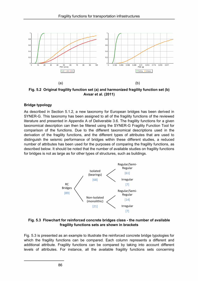
Fragility functions for transportation infrastructures
86
(a) (b)
Fig. 5.2 Original fragility function set (a) and harmonized fragility function set (b) Avsar et al. (2011)
Bridge typology
As described in Section 5.1.2, a new taxonomy for European bridges has been derived in SYNER-G. This taxonomy has been assigned to all of the fragility functions of the reviewed literature and presented in Appendix A of Deliverable 3.6. The fragility functions for a given taxonomical description can then be filtered using the SYNER-G Fragility Function Tool for comparison of the functions. Due to the different taxonomical descriptions used in the derivation of the fragility functions, and the different types of attributes that are used to distinguish the seismic performance of bridges within these different studies, a reduced number of attributes has been used for the purposes of comparing the fragility functions, as described below. It should be noted that the number of available studies on fragility functions for bridges is not as large as for other types of structures, such as buildings.
Fig. 5.3 Flowchart for reinforced concrete bridges class - the number of available
fragility functions sets are shown in brackets
Fig. 5.3 is presented as an example to illustrate the reinforced concrete bridge typologies for which the fragility functions can be compared. Each column represents a different and additional attribute. Fragility functions can be compared by taking into account different levels of attributes. For instance, all the available fragility functions sets concerning
LS1 LS2 LS3
PGV [cm/s]1009080706050403020100
Pro
babi
lity
of e
xcee
danc
e
1
0.8
0.6
0.4
0.2
0
Yielding Collapse
PGA [g]0.9170.8160.7140.6120.510.4080.3060.2040.1020
Pro
babi
lity
of e
xcee
danc
e
1
0.8
0.6
0.4
0.2
0
RC Bridges
[89]
Isolated (bearings)
[68]
Regular/Semi-Regular
[61]
Irregular
[7]
Non-Isolated (monolithic)
[21]
Regular/Semi-Regular
[14]
Irregular
[7]
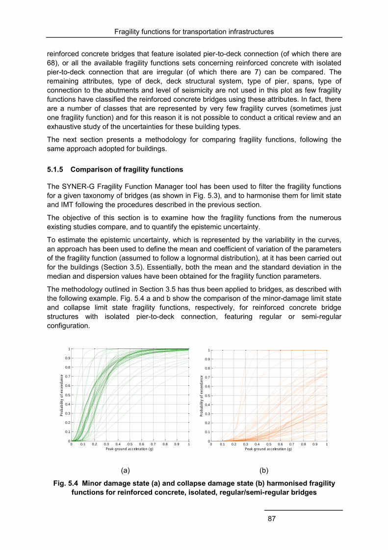
Fragility functions for transportation infrastructures
87
reinforced concrete bridges that feature isolated pier-to-deck connection (of which there are 68), or all the available fragility functions sets concerning reinforced concrete with isolated pier-to-deck connection that are irregular (of which there are 7) can be compared. The remaining attributes, type of deck, deck structural system, type of pier, spans, type of connection to the abutments and level of seismicity are not used in this plot as few fragility functions have classified the reinforced concrete bridges using these attributes. In fact, there are a number of classes that are represented by very few fragility curves (sometimes just one fragility function) and for this reason it is not possible to conduct a critical review and an exhaustive study of the uncertainties for these building types.
The next section presents a methodology for comparing fragility functions, following the same approach adopted for buildings.
5.1.5 Comparison of fragility functions
The SYNER-G Fragility Function Manager tool has been used to filter the fragility functions for a given taxonomy of bridges (as shown in Fig. 5.3), and to harmonise them for limit state and IMT following the procedures described in the previous section.
The objective of this section is to examine how the fragility functions from the numerous existing studies compare, and to quantify the epistemic uncertainty.
To estimate the epistemic uncertainty, which is represented by the variability in the curves, an approach has been used to define the mean and coefficient of variation of the parameters of the fragility function (assumed to follow a lognormal distribution), at it has been carried out for the buildings (Section 3.5). Essentially, both the mean and the standard deviation in the median and dispersion values have been obtained for the fragility function parameters.
The methodology outlined in Section 3.5 has thus been applied to bridges, as described with the following example. Fig. 5.4 a and b show the comparison of the minor-damage limit state and collapse limit state fragility functions, respectively, for reinforced concrete bridge structures with isolated pier-to-deck connection, featuring regular or semi-regular configuration.
(a) (b)
Fig. 5.4 Minor damage state (a) and collapse damage state (b) harmonised fragility functions for reinforced concrete, isolated, regular/semi-regular bridges
0 0.1 0.2 0.3 0.4 0.5 0.6 0.7 0.8 0.9 10
0.1
0.2
0.3
0.4
0.5
0.6
0.7
0.8
0.9
1
Pro
babili
ty o
f exce
edance
Peak ground acceleration (g)
0 0.1 0.2 0.3 0.4 0.5 0.6 0.7 0.8 0.9 10
0.1
0.2
0.3
0.4
0.5
0.6
0.7
0.8
0.9
1
Pro
babili
ty o
f exce
edance
Peak ground acceleration (g)

Fragility functions for transportation infrastructures
88
Fig. 5.5 displays the mean fragility function (based on the mean value of the median/logarithmic mean and mean value of the dispersion/logarithmic standard deviation) together with the individual fragility functions for a reinforced concrete bridge typology (the same group of reinforced concrete, isolated, regular/semi-regular bridges considered in Fig. 5.4). Histograms of the logarithmic mean and logarithmic standard deviation have thus been produced to obtain the aforementioned mean fragility function. In addition, the coefficient of variation from these histograms has been calculated to obtain the standard deviation of the logarithmic mean and the coefficient of variation (cv) of the logarithmic standard deviation. The mean and coefficient of variation (cv) of the lognormal parameters of the fragility functions (i.e. logarithmic mean and logarithmic standard deviation) are shown in Table 5.6.
Table 5.6 Mean and cv of lognormal fragility parameters for a reinforced concrete bridge typology
Reinforced concrete – isolated – regular / semi-regular Minor damage Collapse logarithmi
c mean, μ1 logarithmic standard
deviation, σ1 logarithmic
mean, μ2 logarithmic standard
deviation, σ2
Mean -1.593 0.611 0.052 0.587
cv (%) 27 33 1267 31
(a) (b)
Fig. 5.5 Mean fragility function of minor damage limit state curves (a) and collapse limit state curves (b) for a reinforced concrete bridge group typology
Based on the distribution of the parameters, a correlation coefficient matrix can be computed. Table 5.7 gives the corresponding correlation coefficient matrix for this example.

Fragility functions for transportation infrastructures
89
Table 5.7 Correlation coefficient matrix for a reinforced concrete bridge typology
μ1 σ1 μ2 σ2
μ1 1 -0.172 0.195 0.048 σ1 -0.172 1 -0.266 -0.072 μ2 0.195 -0.266 1 0.688 σ2 0.048 -0.072 0.688 1
The mean and coefficient of variation of the parameters of the lognormal distribution for the yielding and collapse limit state for all the considered bridge typologies based on the fragility functions reviewed in this study, are presented in Appendix C.
5.1.6 Closing remarks
A number of studies related to the fragility of bridges have been reviewed and new fragility curves have been calculated within the Eurocode 8 context. Both existing and new fragility functions have been stored in the Fragility Function Manager tool which is able to collect, harmonize and compare them. Based on this review, the identification of the main reinforced concrete bridge classes in Europe has been obtained and the key parameters that affect their fragility have been identified and used to propose a new taxonomy. The application of the SYNER-G taxonomy proposed in the project to all existing functions has allowed the fragility functions to be grouped together and directly compared. Furthermore, based on the aforementioned grouping, a set of mean fragility functions, with associated uncertainty and correlation coefficient matrix have been proposed for a number of reinforced concrete typologies. This study has revealed the need for more research in this subject as quite limited studies are available compared to buildings and the uncertainties in the parameter of the fragility functions are larger.

Fragility functions for transportation infrastructures
90
5.2 ROADWAY NETWORKS
5.2.1 Identification of main typologies
Roadway elements are categorized as earth structures, therefore a main typological feature is the soil type, which characterizes either a construction or its foundation and surrounding material. Different soil classification systems are available based on various soil properties. A widely used classification scheme is the one provided by Eurocode 8 (EC8, 2004), which is based on the soil’s shear wave velocity, Vs30.
Another important parameter for the description of typology is the hierarchy of roads according to their functions and capacities. In the European project SAFELAND a distinction is made between high speed and local roads based on speed limit and number of lanes.
In addition to the aforementioned main attributes, other important typological features are given in the following for each roadway element:
o Tunnels: The basic parameters for the description of the typology are the construction method (bored or mined, cut-and-cover, immersed), the shape (circular, rectangular, horseshoe etc.), the depth (surface, shallow, deep), the geological conditions (rock, alluvial), and supporting system (concrete, masonry, steel etc.);
o Embankments, trenches and slopes: The main typological features considered in this project are the geometrical parameters of the construction (i.e. slope angle, height). These elements are mainly presented in highways (non urban networks);
o Road pavements: The basic parameter is the number of traffic lanes which is based on the functional hierarchy of the network;
o Bridge abutments: The main typological features are the depth and the soil conditions of foundation and fill material behind the abutment. The depth is dependent on the surrounding topography and bridge abutment geometry, while the fill material behaviour depends on its compaction level.
5.2.2 Damage description
Earthquake effects on road elements can be grouped into two categories, 1: ground shaking (expressed often in terms of peak ground acceleration); and 2: ground failure such as liquefaction, fault displacement, and slope instability (expressed in terms of permanent ground deformations).A brief summary is given below for each roadway element:
o Tunnels: Three types of deformations express the response of underground structures to seismic motions (1: axial compression and extension, 2:longitudinal bending and 3:ovaling/racking). Typical damages are (Corigliano, 2007): slope instability leading to tunnel collapse, portal failure, roof or wall collapse, invert uplift spalling, cracking or crushing of the concrete lining, slabbing or spalling of the rock around the opening, bending and buckling of reinforcing bars, pavement cracks, wall deformation, local opening of joints and obstruction of the opening, opening deformations.
o Embankments: When the foundation bearing capacity is lost due to static and dynamic loading, for example due to soil liquefaction, the embankment may spread

Fragility functions for transportation infrastructures
91
laterally and settle at the same time. This could lead to lateral movement of embankment (from a few centimetres to several meters) and opening of cracks in the road pavement.
o Trenches and slopes: Earthquake induced landslides can cause partial or complete blockage of the road as well as the structural damage to the road pavement. In addition to these types of damages in embankments, roads constructed in trenches and on slopes are subjected to failures of the slopes beside the road.
o Road pavement: Damages to road pavement can be direct (e.g. fault ruptures, settlement, lateral spreading), indirect (e.g. collapsed buildings, landslide debris, damage to underlying pipelines) or induced (e.g. restoration works).
o Bridge abutments/retaining walls: Approach fills alongside bridge abutments/retaining walls are vulnerable to damage from earthquake-induced differential settlement. Approach-fill settlement has been the most commonly occurring type of highway system damage during recent earthquakes. It does not often result in extensive repair costs; however, it disrupts the functionality of the road network.
Different damage criteria have been proposed for the fragility analysis of roadway elements. The number of damage states is variable and in some cases is related with the functionality/traffic state or/and the repair duration and cost. In empirical and expert judgment methods, the extent of damage is described qualitatively (e.g. extent of cracks or settlements). In numerical methods the damage levels are defined based on the range of a specific damage index (e.g. permanent ground deformation, capacity, factor of safety). Damage criteria proposed by different studies are summarized in the next section.
Fig. 5.6 Road embankment failure caused by lateral slumping during the 1995 Kozani
(GR) earthquake (left) and damage of pavement during the 2003 Lefkas (GR) earthquake caused by subsidence due to soil liquefaction (right)
5.2.3 State of the art fragility functions for roadway components
A summary review of existing fragility functions for roadway elements is presented in Table 5.8 to Table 5.13. The proposed methodologies, classification schemes, intensity measure types (IMT) and damage states are outlined. Based on this review, it was decided to develop new numerical fragility curves for the following cases: a) urban tunnels in alluvial deposits, b)

Fragility functions for transportation infrastructures
92
embankments/trenches, and c) bridge abutments. For other elements such as road pavements, slopes and highway (rock/alluvial) tunnels, the existing fragility methods are adopted or modified.
Table 5.8 Summary review of existing fragility functions for embankments
Reference Methodology Classification IMT Damage States Maruyama
et al., 2008, 2010
Empirical. Damage datasets from 2003
Northern-Miyagi, 2003 Tokachi-oki,
2004 Niigata Chuetsu, 2007 Niigata Chuetsu-
oki earthquakes Log-normal distribution
Japanese expressways embankments (height: 5-10
m)
Peak Ground Velocity
Major damage (affecting the
serviceability of traffic). All damage.
Damage ratio: number of damage incidents per km of
expressway embankment
Lagaros et al., 2009
Analytical. Pseudostatic slope stability analyses,
Monte Carlo simulation method and neural
network meta models.
Trapezoid embankment (deterministic and random variables of dimensions)
Peak Ground Acceleration
(ground shaking)
Slight, moderate, extensive, collapse
Damage index: Factor of Safety
Table 5.9 Summary review of existing fragility functions for slopes
Reference Methodology Classification IMT Damage States SAFELAND (Pitilakis
et al., 2010)
Modified HAZUS (NIBS 2004) curves based on Bray and Travasarou (2007)
model. Log-normal cumulative
distributions.
Major/highway roads (4 or more
lanes) Urban roads (2
traffic lanes) Slope is described
through yield coefficient (ky)
Peak Ground Accel. (PGA)
(ground shaking)
Slight/minor (DS1), moderate (DS2), extensive/ complete (DS3)
Description: Extent of ground
movement
ATC-13, 1985
Slope failure probability matrices,
Expert judgment
6 slope classes, defined by critical acceleration, ac.
Modified Mercalli Intensity
Light, Moderate, Heavy, Severe,
Catastrophic
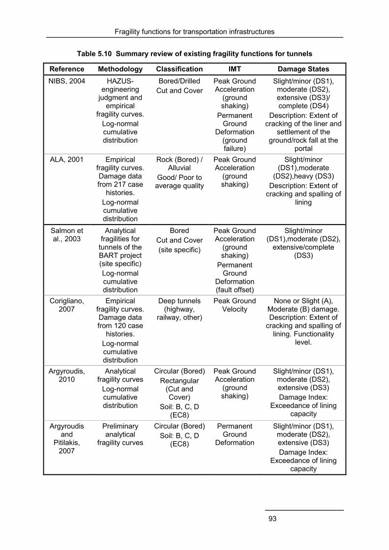
Fragility functions for transportation infrastructures
93
Table 5.10 Summary review of existing fragility functions for tunnels
Reference Methodology Classification IMT Damage States NIBS, 2004 HAZUS-
engineering judgment and
empirical fragility curves.
Log-normal cumulative distribution
Bored/Drilled Cut and Cover
Peak Ground Acceleration
(ground shaking)
Permanent Ground
Deformation (ground failure)
Slight/minor (DS1), moderate (DS2), extensive (DS3)/ complete (DS4)
Description: Extent of cracking of the liner and
settlement of the ground/rock fall at the
portal ALA, 2001 Empirical
fragility curves. Damage data from 217 case
histories. Log-normal cumulative distribution
Rock (Bored) / Alluvial
Good/ Poor to average quality
Peak Ground Acceleration
(ground shaking)
Slight/minor (DS1),moderate
(DS2),heavy (DS3) Description: Extent of
cracking and spalling of lining
Salmon et al., 2003
Analytical fragilities for
tunnels of the BART project (site specific) Log-normal cumulative distribution
Bored Cut and Cover (site specific)
Peak Ground Acceleration
(ground shaking)
Permanent Ground
Deformation (fault offset)
Slight/minor (DS1),moderate (DS2),
extensive/complete (DS3)
Corigliano, 2007
Empirical fragility curves. Damage data from 120 case
histories. Log-normal cumulative distribution
Deep tunnels (highway,
railway, other)
Peak Ground Velocity
None or Slight (A), Moderate (B) damage. Description: Extent of
cracking and spalling of lining. Functionality
level.
Argyroudis, 2010
Analytical fragility curves
Log-normal cumulative distribution
Circular (Bored) Rectangular
(Cut and Cover)
Soil: B, C, D (EC8)
Peak Ground Acceleration
(ground shaking)
Slight/minor (DS1), moderate (DS2), extensive (DS3) Damage Index:
Exceedance of lining capacity
Argyroudis and
Pitilakis, 2007
Preliminary analytical
fragility curves
Circular (Bored) Soil: B, C, D
(EC8)
Permanent Ground
Deformation
Slight/minor (DS1), moderate (DS2), extensive (DS3) Damage Index:
Exceedance of lining capacity
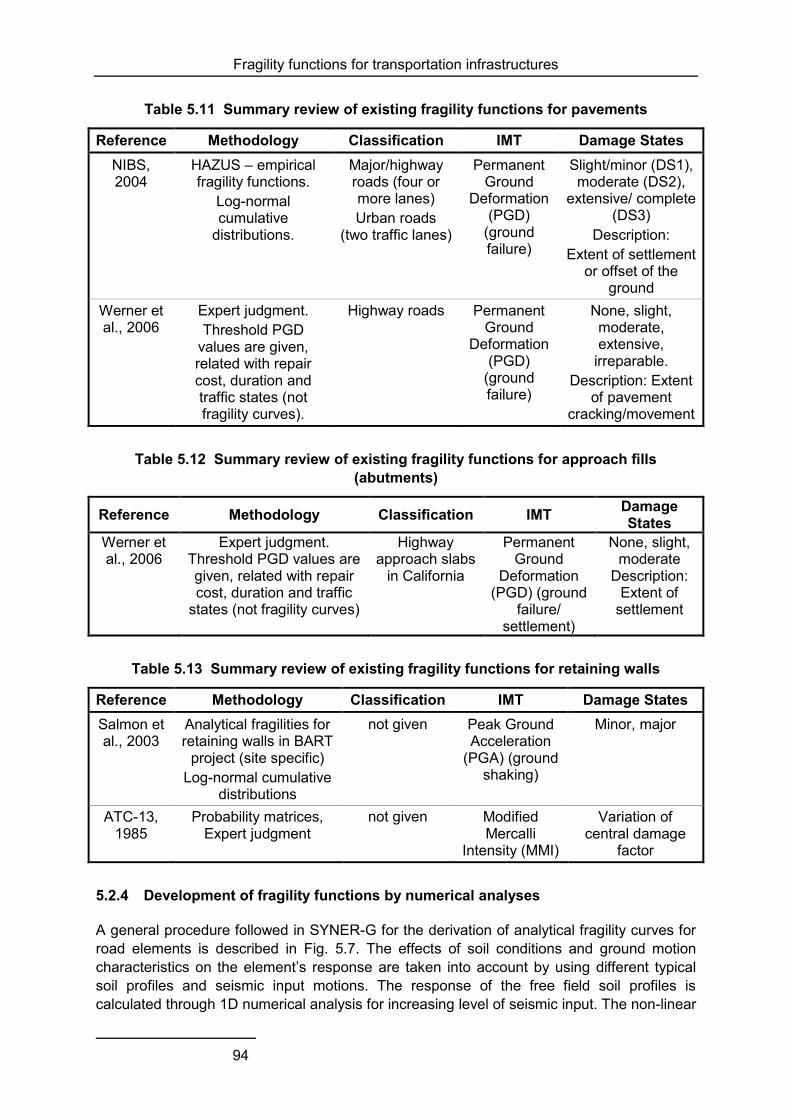
Fragility functions for transportation infrastructures
94
Table 5.11 Summary review of existing fragility functions for pavements
Reference Methodology Classification IMT Damage States NIBS, 2004
HAZUS – empirical fragility functions.
Log-normal cumulative
distributions.
Major/highway roads (four or more lanes) Urban roads
(two traffic lanes)
Permanent Ground
Deformation (PGD)
(ground failure)
Slight/minor (DS1), moderate (DS2),
extensive/ complete (DS3)
Description: Extent of settlement
or offset of the ground
Werner et al., 2006
Expert judgment. Threshold PGD
values are given, related with repair cost, duration and traffic states (not fragility curves).
Highway roads Permanent Ground
Deformation (PGD)
(ground failure)
None, slight, moderate, extensive,
irreparable. Description: Extent
of pavement cracking/movement
Table 5.12 Summary review of existing fragility functions for approach fills (abutments)
Reference Methodology Classification IMT Damage States
Werner et al., 2006
Expert judgment. Threshold PGD values are given, related with repair cost, duration and traffic
states (not fragility curves)
Highway approach slabs
in California
Permanent Ground
Deformation (PGD) (ground
failure/ settlement)
None, slight, moderate
Description: Extent of
settlement
Table 5.13 Summary review of existing fragility functions for retaining walls
Reference Methodology Classification IMT Damage States Salmon et al., 2003
Analytical fragilities for retaining walls in BART
project (site specific) Log-normal cumulative
distributions
not given Peak Ground Acceleration
(PGA) (ground shaking)
Minor, major
ATC-13, 1985
Probability matrices, Expert judgment
not given Modified Mercalli
Intensity (MMI)
Variation of central damage
factor
5.2.4 Development of fragility functions by numerical analyses
A general procedure followed in SYNER-G for the derivation of analytical fragility curves for road elements is described in Fig. 5.7. The effects of soil conditions and ground motion characteristics on the element’s response are taken into account by using different typical soil profiles and seismic input motions. The response of the free field soil profiles is calculated through 1D numerical analysis for increasing level of seismic input. The non-linear
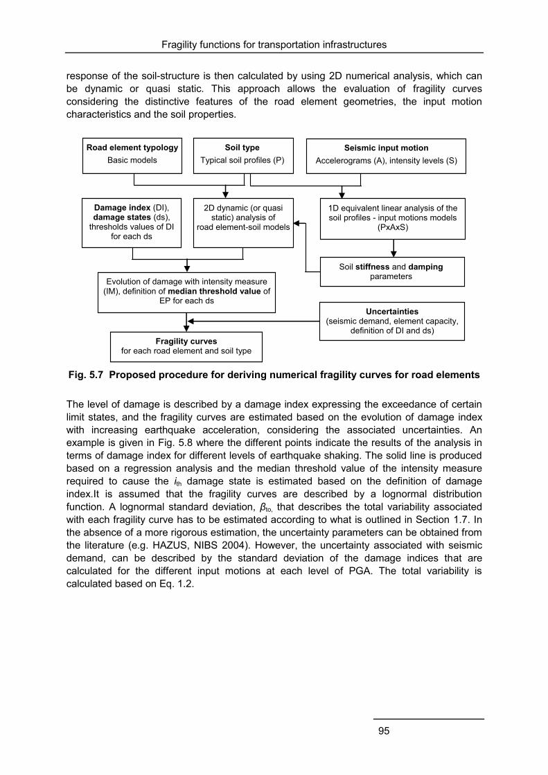
Fragility functions for transportation infrastructures
95
response of the soil-structure is then calculated by using 2D numerical analysis, which can be dynamic or quasi static. This approach allows the evaluation of fragility curves considering the distinctive features of the road element geometries, the input motion characteristics and the soil properties.
Fig. 5.7 Proposed procedure for deriving numerical fragility curves for road elements
The level of damage is described by a damage index expressing the exceedance of certain limit states, and the fragility curves are estimated based on the evolution of damage index with increasing earthquake acceleration, considering the associated uncertainties. An example is given in Fig. 5.8 where the different points indicate the results of the analysis in terms of damage index for different levels of earthquake shaking. The solid line is produced based on a regression analysis and the median threshold value of the intensity measure required to cause the ith damage state is estimated based on the definition of damage index.It is assumed that the fragility curves are described by a lognormal distribution function. A lognormal standard deviation, βto, that describes the total variability associated with each fragility curve has to be estimated according to what is outlined in Section 1.7. In the absence of a more rigorous estimation, the uncertainty parameters can be obtained from the literature (e.g. HAZUS, NIBS 2004). However, the uncertainty associated with seismic demand, can be described by the standard deviation of the damage indices that are calculated for the different input motions at each level of PGA. The total variability is calculated based on Eq. 1.2.
Road element typology Basic models
Soil type Typical soil profiles (P)
Seismic input motion Accelerograms (A), intensity levels (S)
1D equivalent linear analysis of the soil profiles - input motions models
(PxAxS)
2D dynamic (or quasi static) analysis of
road element-soil models
Soil stiffness and damping parameters
Damage index (DI), damage states (ds),
thresholds values of DI for each ds
Evolution of damage with intensity measure (IM), definition of median threshold value of
EP for each ds
Fragility curves for each road element and soil type
Uncertainties (seismic demand, element capacity,
definition of DI and ds)
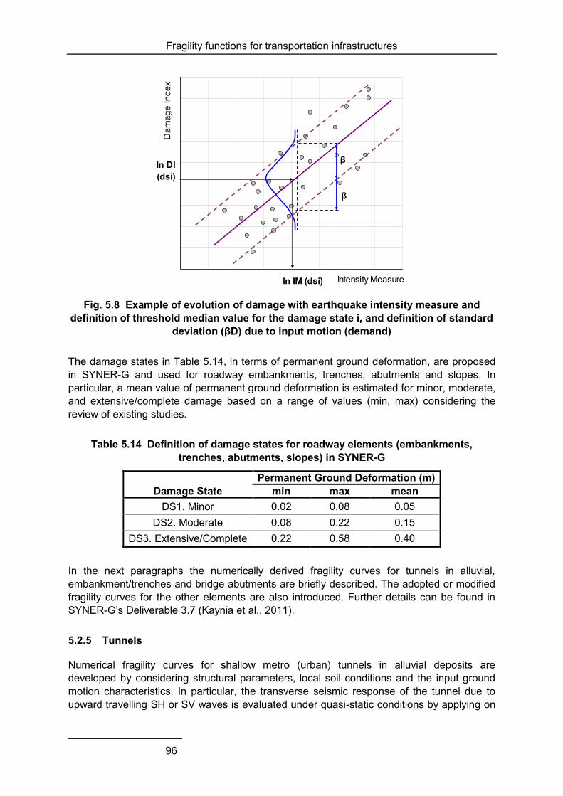
Fragility functions for transportation infrastructures
96
Fig. 5.8 Example of evolution of damage with earthquake intensity measure and
definition of threshold median value for the damage state i, and definition of standard deviation (βD) due to input motion (demand)
The damage states in Table 5.14, in terms of permanent ground deformation, are proposed in SYNER-G and used for roadway embankments, trenches, abutments and slopes. In particular, a mean value of permanent ground deformation is estimated for minor, moderate, and extensive/complete damage based on a range of values (min, max) considering the review of existing studies.
Table 5.14 Definition of damage states for roadway elements (embankments, trenches, abutments, slopes) in SYNER-G
Permanent Ground Deformation (m) Damage State min max mean
DS1. Minor 0.02 0.08 0.05 DS2. Moderate 0.08 0.22 0.15
DS3. Extensive/Complete 0.22 0.58 0.40
In the next paragraphs the numerically derived fragility curves for tunnels in alluvial, embankment/trenches and bridge abutments are briefly described. The adopted or modified fragility curves for the other elements are also introduced. Further details can be found in SYNER-G’s Deliverable 3.7 (Kaynia et al., 2011).
5.2.5 Tunnels
Numerical fragility curves for shallow metro (urban) tunnels in alluvial deposits are developed by considering structural parameters, local soil conditions and the input ground motion characteristics. In particular, the transverse seismic response of the tunnel due to upward travelling SH or SV waves is evaluated under quasi-static conditions by applying on
Intensity Measure
Dam
age
Inde
x 1
ln IM (dsi)
ln DI (dsi)
β
β
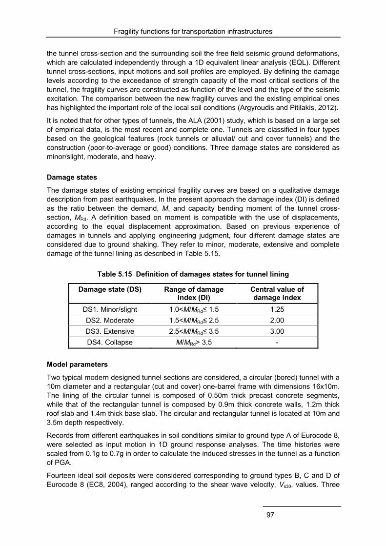
Fragility functions for transportation infrastructures
97
the tunnel cross-section and the surrounding soil the free field seismic ground deformations, which are calculated independently through a 1D equivalent linear analysis (EQL). Different tunnel cross-sections, input motions and soil profiles are employed. By defining the damage levels according to the exceedance of strength capacity of the most critical sections of the tunnel, the fragility curves are constructed as function of the level and the type of the seismic excitation. The comparison between the new fragility curves and the existing empirical ones has highlighted the important role of the local soil conditions (Argyroudis and Pitilakis, 2012).
It is noted that for other types of tunnels, the ALA (2001) study, which is based on a large set of empirical data, is the most recent and complete one. Tunnels are classified in four types based on the geological features (rock tunnels or alluvial/ cut and cover tunnels) and the construction (poor-to-average or good) conditions. Three damage states are considered as minor/slight, moderate, and heavy.
Damage states
The damage states of existing empirical fragility curves are based on a qualitative damage description from past earthquakes. In the present approach the damage index (DI) is defined as the ratio between the demand, M, and capacity bending moment of the tunnel cross-section, MRd. A definition based on moment is compatible with the use of displacements, according to the equal displacement approximation. Based on previous experience of damages in tunnels and applying engineering judgment, four different damage states are considered due to ground shaking. They refer to minor, moderate, extensive and complete damage of the tunnel lining as described in Table 5.15.
Table 5.15 Definition of damages states for tunnel lining
Damage state (DS) Range of damage index (DI)
Central value of damage index
DS1. Minor/slight 1.0<Μ/ΜRd≤ 1.5 1.25 DS2. Moderate 1.5<Μ/ΜRd≤ 2.5 2.00 DS3. Extensive 2.5<Μ/ΜRd≤ 3.5 3.00 DS4. Collapse Μ/ΜRd> 3.5 -
Model parameters
Two typical modern designed tunnel sections are considered, a circular (bored) tunnel with a 10m diameter and a rectangular (cut and cover) one-barrel frame with dimensions 16x10m. The lining of the circular tunnel is composed of 0.50m thick precast concrete segments, while that of the rectangular tunnel is composed by 0.9m thick concrete walls, 1.2m thick roof slab and 1.4m thick base slab. The circular and rectangular tunnel is located at 10m and 3.5m depth respectively.
Records from different earthquakes in soil conditions similar to ground type A of Eurocode 8, were selected as input motion in 1D ground response analyses. The time histories were scaled from 0.1g to 0.7g in order to calculate the induced stresses in the tunnel as a function of PGA.
Fourteen ideal soil deposits were considered corresponding to ground types B, C and D of Eurocode 8 (EC8, 2004), ranged according to the shear wave velocity, Vs30, values. Three
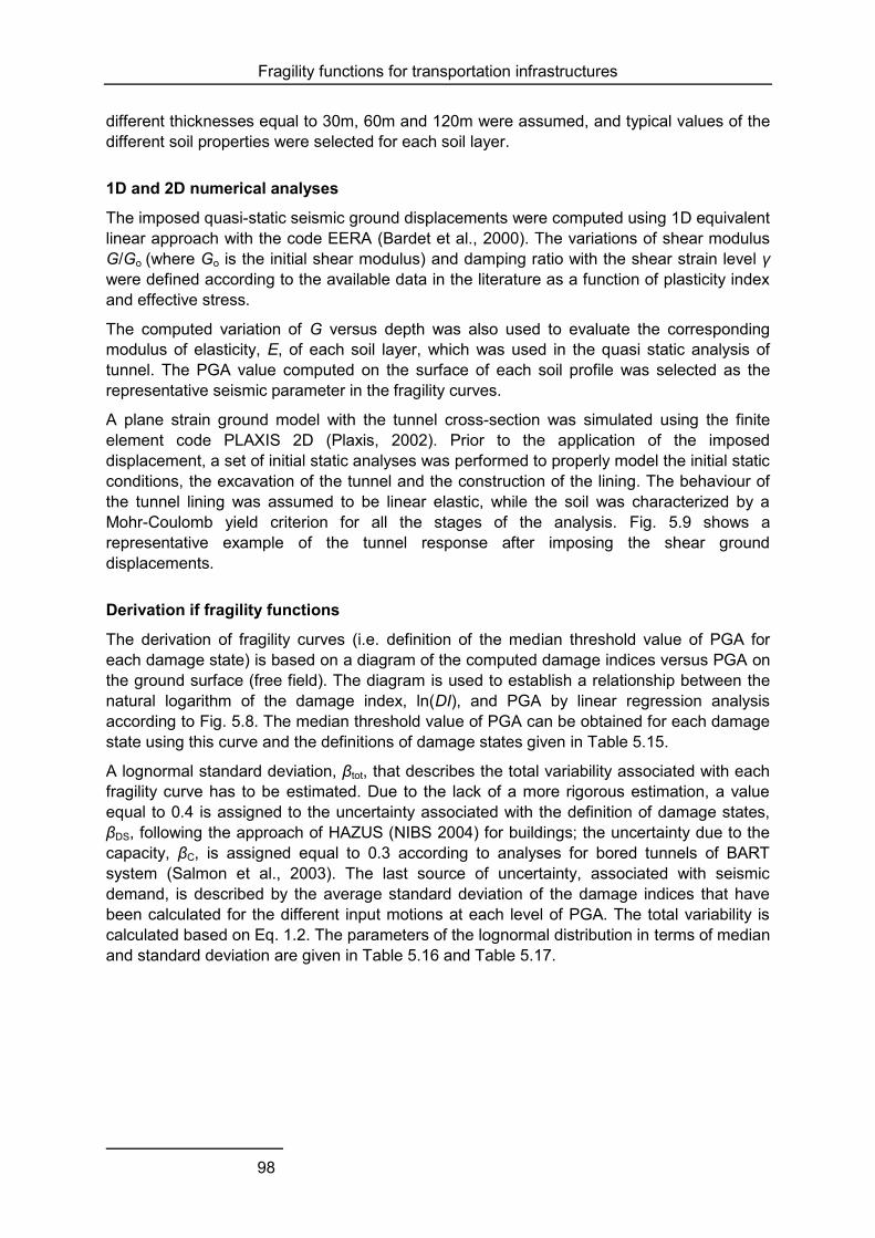
Fragility functions for transportation infrastructures
98
different thicknesses equal to 30m, 60m and 120m were assumed, and typical values of the different soil properties were selected for each soil layer.
1D and 2D numerical analyses
The imposed quasi-static seismic ground displacements were computed using 1D equivalent linear approach with the code EERA (Bardet et al., 2000). The variations of shear modulus G/Go (where Go is the initial shear modulus) and damping ratio with the shear strain level γ were defined according to the available data in the literature as a function of plasticity index and effective stress.
The computed variation of G versus depth was also used to evaluate the corresponding modulus of elasticity, E, of each soil layer, which was used in the quasi static analysis of tunnel. The PGA value computed on the surface of each soil profile was selected as the representative seismic parameter in the fragility curves.
A plane strain ground model with the tunnel cross-section was simulated using the finite element code PLAXIS 2D (Plaxis, 2002). Prior to the application of the imposed displacement, a set of initial static analyses was performed to properly model the initial static conditions, the excavation of the tunnel and the construction of the lining. The behaviour of the tunnel lining was assumed to be linear elastic, while the soil was characterized by a Mohr-Coulomb yield criterion for all the stages of the analysis. Fig. 5.9 shows a representative example of the tunnel response after imposing the shear ground displacements.
Derivation if fragility functions
The derivation of fragility curves (i.e. definition of the median threshold value of PGA for each damage state) is based on a diagram of the computed damage indices versus PGA on the ground surface (free field). The diagram is used to establish a relationship between the natural logarithm of the damage index, ln(DI), and PGA by linear regression analysis according to Fig. 5.8. The median threshold value of PGA can be obtained for each damage state using this curve and the definitions of damage states given in Table 5.15.
A lognormal standard deviation, βtot, that describes the total variability associated with each fragility curve has to be estimated. Due to the lack of a more rigorous estimation, a value equal to 0.4 is assigned to the uncertainty associated with the definition of damage states, βDS, following the approach of HAZUS (NIBS 2004) for buildings; the uncertainty due to the capacity, βC, is assigned equal to 0.3 according to analyses for bored tunnels of BART system (Salmon et al., 2003). The last source of uncertainty, associated with seismic demand, is described by the average standard deviation of the damage indices that have been calculated for the different input motions at each level of PGA. The total variability is calculated based on Eq. 1.2. The parameters of the lognormal distribution in terms of median and standard deviation are given in Table 5.16 and Table 5.17.
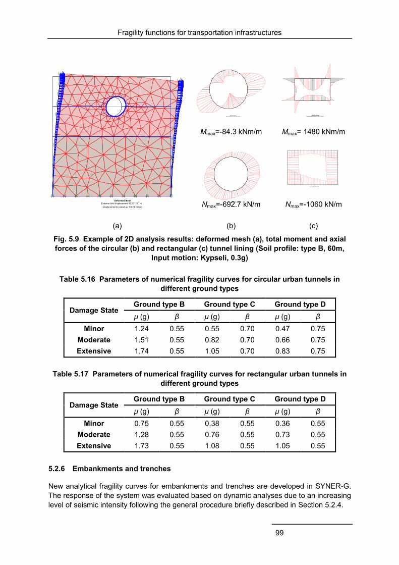
Fragility functions for transportation infrastructures
99
(a)
Mmax=-84.3 kNm/m
Mmax= 1480 kNm/m
Nmax=-692.7 kN/m
(b)
Nmax=-1060 kN/m
(c)
Fig. 5.9 Example of 2D analysis results: deformed mesh (a), total moment and axial forces of the circular (b) and rectangular (c) tunnel lining (Soil profile: type B, 60m,
Input motion: Kypseli, 0.3g)
Table 5.16 Parameters of numerical fragility curves for circular urban tunnels in different ground types
Damage State Ground type B Ground type C Ground type D μ (g) β μ (g) β μ (g) β
Minor 1.24 0.55 0.55 0.70 0.47 0.75 Moderate 1.51 0.55 0.82 0.70 0.66 0.75 Extensive 1.74 0.55 1.05 0.70 0.83 0.75
Table 5.17 Parameters of numerical fragility curves for rectangular urban tunnels in different ground types
Damage State Ground type B Ground type C Ground type D μ (g) β μ (g) β μ (g) β
Minor 0.75 0.55 0.38 0.55 0.36 0.55 Moderate 1.28 0.55 0.76 0.55 0.73 0.55 Extensive 1.73 0.55 1.08 0.55 1.05 0.55
5.2.6 Embankments and trenches
New analytical fragility curves for embankments and trenches are developed in SYNER-G. The response of the system was evaluated based on dynamic analyses due to an increasing level of seismic intensity following the general procedure briefly described in Section 5.2.4.
Deformed MeshExtreme total displacement 43.07*10-3 m
(displacements scaled up 100.00 times)
Bending momentExtreme bending moment -84.28 kNm/m
Bending momentExtreme bending moment 1.48*103 kNm/m
Axial forcesExtreme axial force -692.68 kN/m
Axial forcesExtreme axial force -1.06*103 kN/m

Fragility functions for transportation infrastructures
100
Model parameters
Representative geometries are considered with heights equal to 2.0 mand 4.0m for the embankment and 4.0 m and 6.0m for the trench.
Five real records from different earthquakes, in soil conditions similar to ground types A (rock) or B (stiff soil) of Eurocode 8, were selected as input motion in outcrop conditions for the analyses. The records are: Kocaeli 1999, Gebze; Hector Mine 1999, Hector; Parnitha 1999, Kypseli; Loma Prieta 1989, Diamond Height; and Umbria Marche 1998, Cubbio-Piene. The time histories were scaled from 0.1g to 0.7g in order to calculate the response of embankment/trench as a function of PGA.
Two ideal soil deposits of 50m were considered, corresponding to ground types C and D with shear wave velocity (Vs30) in the range defined by Eurocode 8. Typical values of soil properties were selected for the embankment.
The numerical simulations were performed with the finite element code PLAXIS 2D v9.02 (Plaxis 2008). A close-up of the model is shown in Fig. 5.10. The total width of the model is equal to 500m, which is sufficiently large to avoid boundary reflections.
Fig. 5.10 Finite element mesh used in the analyses of embankment
Derivation if fragility functions
The derivation of fragility curves is based on a diagram of the computed damage indices (average total permanent ground displacement, PGD, on embankment) versus PGA on the ground surface (see Fig. 5.8). A relationship is established by linear regression analysis, considering PGD as the dependent variable and PGA as the independent variable. The median threshold value of PGA can be obtained for each damage state based on the aforementioned diagram and the definitions given in Table 5.14. A lognormal standard deviation, β, that describes the total variability associated with each fragility curve was estimated as described in Section 5.2.4.The estimated parameters of the fragility curves are presented in Table 5.18 and Table 5.19. For details see Kaynia et al. (2011).
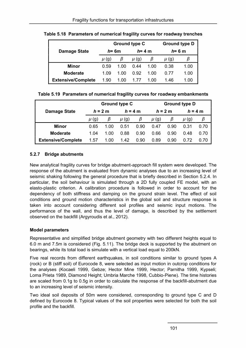
Fragility functions for transportation infrastructures
101
Table 5.18 Parameters of numerical fragility curves for roadway trenches
Damage State Ground type C Ground type D
h= 6m h= 4 m h= 6 m μ (g) β μ (g) β μ (g) β
Minor 0.59 1.00 0.44 1.00 0.38 1.00 Moderate 1.09 1.00 0.92 1.00 0.77 1.00
Extensive/Complete 1.90 1.00 1.77 1.00 1.46 1.00
Table 5.19 Parameters of numerical fragility curves for roadway embankments
Damage State Ground type C Ground type D
h = 2 m h = 4 m h = 2 m h = 4 m μ (g) β μ (g) β μ (g) β μ (g) β
Minor 0.65 1.00 0.51 0.90 0.47 0.90 0.31 0.70 Moderate 1.04 1.00 0.88 0.90 0.66 0.90 0.48 0.70
Extensive/Complete 1.57 1.00 1.42 0.90 0.89 0.90 0.72 0.70
5.2.7 Bridge abutments
New analytical fragility curves for bridge abutment-approach fill system were developed. The response of the abutment is evaluated from dynamic analyses due to an increasing level of seismic shaking following the general procedure that is briefly described in Section 5.2.4. In particular, the soil behaviour is simulated through a 2D fully coupled FE model, with an elasto-plastic criterion. A calibration procedure is followed in order to account for the dependency of both stiffness and damping on the ground strain level. The effect of soil conditions and ground motion characteristics in the global soil and structure response is taken into account considering different soil profiles and seismic input motions. The performance of the wall, and thus the level of damage, is described by the settlement observed on the backfill (Argyroudis et al., 2012).
Model parameters
Representative and simplified bridge abutment geometry with two different heights equal to 6.0 m and 7.5m is considered (Fig. 5.11). The bridge deck is supported by the abutment on bearings, while its total load is simulate with a vertical load equal to 200kN.
Five real records from different earthquakes, in soil conditions similar to ground types A (rock) or B (stiff soil) of Eurocode 8, were selected as input motion in outcrop conditions for the analyses (Kocaeli 1999, Gebze; Hector Mine 1999, Hector; Parnitha 1999, Kypseli; Loma Prieta 1989, Diamond Height; Umbria Marche 1998, Cubbio-Piene). The time histories are scaled from 0.1g to 0.5g in order to calculate the response of the backfill-abutment due to an increasing level of seismic intensity.
Two ideal soil deposits of 50m were considered, corresponding to ground type C and D defined by Eurocode 8. Typical values of the soil properties were selected for both the soil profile and the backfill.

Fragility functions for transportation infrastructures
102
The 1D ground response analyses we performed using 1D equivalent linear approach with the code EERA (Bardet et al., 2000). A calibration procedure was followed in order to account for the dependency of both stiffness and damping on the strain level.
The numerical analyses were performed with the finite element code PLAXIS 2D v9.02 (Plaxis 2008). A close-up of the mesh employed in the study is shown in Fig. 5.12. The total width of the model is equal to 500m, which is sufficient to avoid boundary reflections. All analyses were carried out performing a set of initial static stages to simulate the initial weight, the installation of the abutment and the backfill, followed by the dynamic analyses.
L (m) h (m) H (m) t1 (m) t2 (m) t3 (m) γb (kN/m3) E (kN/m2)
5.5
6.5
6.0
7.5
50.0
50.0
1.0
1.0
1.0
1.0
1.5
2.5
24.0 3.5E+07
* γb: unit weight of concrete
Fig. 5.11 Properties of soil/backfill/abutment under study
Fig. 5.12 Finite element mesh used in the analyses of bridge abutment
t2
t3
L
h
Backfill
Bedrock
SoilH
t1
200kN
EQ
Bridge deck

Fragility functions for transportation infrastructures
103
Derivation if fragility functions
The derivation of fragility curves from the results of the numerical simulations is similar to that presented in the previous section. The estimated parameters of the fragility curves are presented in Table 5.20. It is noted that the fragility curves for complete damage were derived based on extrapolation of the available computation results.
Table 5.20 Parameters of numerical fragility curves for roadway abutments
Damage State Ground type C Ground type D
h= 6 m h= 7.5 m h= 6 m h= 7.5 m μ (g) β μ (g) β μ (g) β μ (g) β
Minor 0.38 0.70 0.26 0.70 0.20 0.90 0.18 0.90 Moderate 0.64 0.70 0.52 0.70 0.45 0.90 0.39 0.90
Extensive/Complete 1.02 0.70 0.97 0.70 0.93 0.90 0.78 0.90
5.2.8 Slopes
The approach described in European project SAFELAND for roads on slopes (Pitilakis et al., 2010) is adapted here. The approach is similar to that used for embankments, trenches and abutments. The difference is that instead of performing numerical simulations, the empirical model by Bray and Travasarou (2007) is used to relate PGA and PGD, considering the characteristics of the slope (quantified by the yield coefficient, ky). The fragility curves are provided in Table 5.21 for different values of ky (equal to 0.05, 0.1, 0.2, 0.3) and a given earthquake magnitude (M = 7.0).
Table 5.21 Parameters of fragility curves for roads on slope
Damage State ky = 0.05 ky = 0.1 ky = 0.2 ky = 0.3
μ (g) β μ (g) β μ (g) β μ (g) β Minor 0.14 0.40 0.25 0.35 0.45 0.35 0.64 0.30
Moderate 0.22 0.40 0.40 0.35 0.71 0.35 1.00 0.30 Extensive/Complete 0.37 0.40 0.64 0.35 1.11 0.35 1.55 0.30
5.2.9 Road pavements (ground failure)
The fragility functions given in HAZUS (NIBS, 2004) are the only functions available in the literature for road pavements. These have resulted from a combination of expert judgment and empirical models, and have shown to give realistic assessment of the expected damage level (Azevedo et al., 2010). Two different types of curves are given: a) for roads with two traffic lanes (urban roads) and b) for roads with four or more lanes (major/highway roads). They are defined with respect to road classification and PGD due to landslides, liquefaction and fault rupture (Table 5.22).
These curves have been validated in SYNER-G using observed damages in road pavements during past earthquakes in Greece. The damages (i.e. cracks of pavement due to settlement or lateral spreading) were recorded in roads with one or two traffic lanes. The

Fragility functions for transportation infrastructures
104
exceedance and occurrence probability of each damage state is calculated for the given (recorded) range of permanent ground deformation using the parameters of the fragility curves. The damage state with the highest probability of occurrence is compared with the observed damage. The results indicate a good agreement between the estimated and observed damage states. Therefore, the existing fragility curves for the roads with two traffic lanes, which is the common case in urban areas, are considered satisfactory and reliable.
Table 5.22 Parameters of numerical fragility curves for road pavements
Damage State
Permanent Ground Deformation, PGD (m) 2 traffic lanes (Urban roads)
≥ 4 traffic lanes (Major roads)
Lognormal standard deviation, β
Minor 0.15 0.30 0.70 Moderate 0.30 0.60 0.70 Extensive 0.60 1.50 0.70
5.2.10 Summary of the proposed fragility functions
The proposed fragility functions for road elements are outlined in Table 5.23. The parameters of these curves, together with their plots, are summarized in Appendix C. Damage scale definitions are also related to the serviceability of the components in terms of functionality and repair capability.
Table 5.23 Summary of proposed fragility functions for road elements
Element Methodology Classification IMT
Urban tunnels in alluvial
SYNER-G Numerical analysis
Ground type: B, C, D (EC8) Circular (bored)
Rectangular (cut and cover) PGA
Other tunnels
ALA, 2001 Empirical
Rock or Alluvial/ Cut and Cover Good or poor to average
construction and conditions PGA
Embankment (road on)
SYNER-G Numerical analysis
Ground type: C, D (EC8) Height: 2.0, 4.0 m
PGA
Trenches (road in)
SYNER-G Numerical analysis
Ground type: C, D (EC8) Height: 2.0, 4.0 m
PGA
Bridge abutments
SYNER-G Numerical analysis
Ground type: C, D (EC8) Height: 6.0, 7.5m
PGA
Slopes SAFELAND
Expert judgement/ Empirical
yield coefficient, ky
earthquake magnitude PGA
Road pavements
HAZUS Expert judgement
2 traffic lanes (Urban roads) >= 4 traffic lanes (Major roads)
PGD
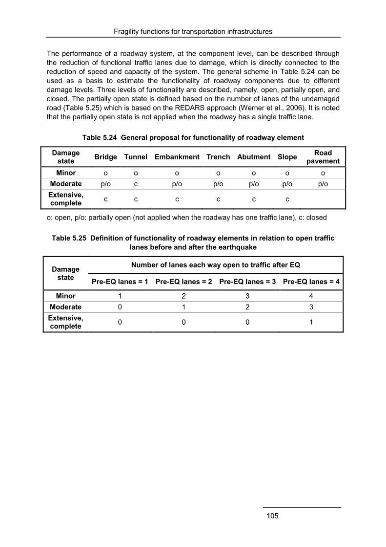
Fragility functions for transportation infrastructures
105
The performance of a roadway system, at the component level, can be described through the reduction of functional traffic lanes due to damage, which is directly connected to the reduction of speed and capacity of the system. The general scheme in Table 5.24 can be used as a basis to estimate the functionality of roadway components due to different damage levels. Three levels of functionality are described, namely, open, partially open, and closed. The partially open state is defined based on the number of lanes of the undamaged road (Table 5.25) which is based on the REDARS approach (Werner et al., 2006). It is noted that the partially open state is not applied when the roadway has a single traffic lane.
Table 5.24 General proposal for functionality of roadway element
Damage state Bridge Tunnel Embankment Trench Abutment Slope Road
pavement Minor o o o o o o o
Moderate p/o c p/o p/o p/o p/o p/o Extensive, complete c c c c c c
o: open, p/o: partially open (not applied when the roadway has one traffic lane), c: closed
Table 5.25 Definition of functionality of roadway elements in relation to open traffic lanes before and after the earthquake
Damage state
Number of lanes each way open to traffic after EQ
Pre-EQ lanes = 1 Pre-EQ lanes = 2 Pre-EQ lanes = 3 Pre-EQ lanes = 4
Minor 1 2 3 4 Moderate 0 1 2 3 Extensive, complete 0 0 0 1

Fragility functions for transportation infrastructures
106
5.3 RAILWAY NETWORKS
5.3.1 Identification of main typologies
Railway tracks are categorized as earth structures; therefore, a main typological feature is the soil type, which characterizes either a construction or its foundation and surrounding material. Different soil classification systems are available based on various soil properties. The soil classification provided by Eurocode 8 is used in this study.
The track is a fundamental part of the railway infrastructure; it consists of elements with different material that transfer static and dynamic loads to the foundation soil. The classical railway track consists of rails and sleepers supported on ballast. The ballast bed rests on a sub-ballast layer which forms the transition layer to the formation. The rails and sleepers are connected by fastenings. These components and other structures such as switches and crossings are all considered parts of the track.
The other railway elements (tunnels, embankments, trenches, slopes and bridge abutments) present similar features as the roadway elements (see Section 5.2).
5.3.2 Damage description
The experience of past earthquakes reveals that railway elements are quite vulnerable to earthquake. Damages to railroads can seriously affect the transportation of products and people in both short- and long- term periods and as a result can have grave economic consequences.
Damage from earthquakes occurs through several mechanisms. Surface displacements across the fault rupture can directly damage facilities that cross the fault. Shaking from seismic waves can derail cars and locomotives, and can damage structures and produce permanent ground movements related to liquefaction and landslides. The latter can cause partial or complete blockage of the railroad as well as the structural damage of the roadbed (Fig. 5.13).
Track damages in past earthquakes have included displaced ballast, broken ties, pulled apart joints, broken rails, buckled rail, large lateral displacements and loss of vertical support for track over appreciable distances (Fig. 5.13). Signal systems have suffered limited damage in relatively low magnitude earthquakes due to broken batteries, overturned electrical relays and wrapped wires in pole lines. Such damage is often highly disruptive but can be quickly repaired. Similar damages might occur in larger earthquakes together with more extensive damages such as broken signal masts (Byers, 2004).
Damage mechanisms for railway tunnels, embankments/trenches, slopes, abutments are similar to these of the roadway elements (see Section 5.2 for description).
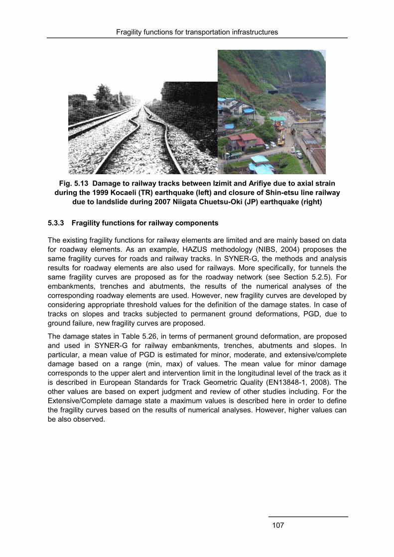
Fragility functions for transportation infrastructures
107
Fig. 5.13 Damage to railway tracks between Izimit and Arifiye due to axial strain
during the 1999 Kocaeli (TR) earthquake (left) and closure of Shin-etsu line railway due to landslide during 2007 Niigata Chuetsu-Oki (JP) earthquake (right)
5.3.3 Fragility functions for railway components
The existing fragility functions for railway elements are limited and are mainly based on data for roadway elements. As an example, HAZUS methodology (NIBS, 2004) proposes the same fragility curves for roads and railway tracks. In SYNER-G, the methods and analysis results for roadway elements are also used for railways. More specifically, for tunnels the same fragility curves are proposed as for the roadway network (see Section 5.2.5). For embankments, trenches and abutments, the results of the numerical analyses of the corresponding roadway elements are used. However, new fragility curves are developed by considering appropriate threshold values for the definition of the damage states. In case of tracks on slopes and tracks subjected to permanent ground deformations, PGD, due to ground failure, new fragility curves are proposed.
The damage states in Table 5.26, in terms of permanent ground deformation, are proposed and used in SYNER-G for railway embankments, trenches, abutments and slopes. In particular, a mean value of PGD is estimated for minor, moderate, and extensive/complete damage based on a range (min, max) of values. The mean value for minor damage corresponds to the upper alert and intervention limit in the longitudinal level of the track as it is described in European Standards for Track Geometric Quality (EN13848-1, 2008). The other values are based on expert judgment and review of other studies including. For the Extensive/Complete damage state a maximum values is described here in order to define the fragility curves based on the results of numerical analyses. However, higher values can be also observed.
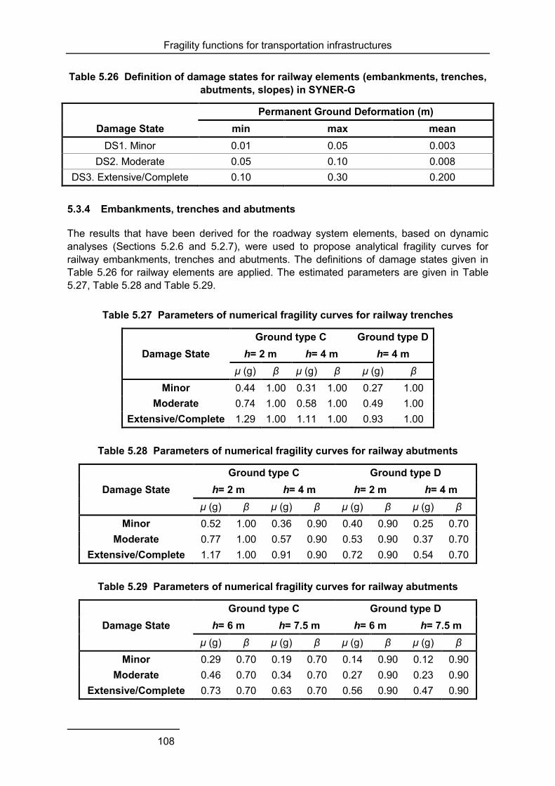
Fragility functions for transportation infrastructures
108
Table 5.26 Definition of damage states for railway elements (embankments, trenches, abutments, slopes) in SYNER-G
Damage State Permanent Ground Deformation (m)
min max mean DS1. Minor 0.01 0.05 0.003
DS2. Moderate 0.05 0.10 0.008 DS3. Extensive/Complete 0.10 0.30 0.200
5.3.4 Embankments, trenches and abutments
The results that have been derived for the roadway system elements, based on dynamic analyses (Sections 5.2.6 and 5.2.7), were used to propose analytical fragility curves for railway embankments, trenches and abutments. The definitions of damage states given in Table 5.26 for railway elements are applied. The estimated parameters are given in Table 5.27, Table 5.28 and Table 5.29.
Table 5.27 Parameters of numerical fragility curves for railway trenches
Damage State Ground type C Ground type D
h= 2 m h= 4 m h= 4 m μ (g) β μ (g) β μ (g) β
Minor 0.44 1.00 0.31 1.00 0.27 1.00 Moderate 0.74 1.00 0.58 1.00 0.49 1.00
Extensive/Complete 1.29 1.00 1.11 1.00 0.93 1.00
Table 5.28 Parameters of numerical fragility curves for railway abutments
Damage State Ground type C Ground type D
h= 2 m h= 4 m h= 2 m h= 4 m μ (g) β μ (g) β μ (g) β μ (g) β
Minor 0.52 1.00 0.36 0.90 0.40 0.90 0.25 0.70 Moderate 0.77 1.00 0.57 0.90 0.53 0.90 0.37 0.70
Extensive/Complete 1.17 1.00 0.91 0.90 0.72 0.90 0.54 0.70
Table 5.29 Parameters of numerical fragility curves for railway abutments
Damage State Ground type C Ground type D
h= 6 m h= 7.5 m h= 6 m h= 7.5 m μ (g) β μ (g) β μ (g) β μ (g) β
Minor 0.29 0.70 0.19 0.70 0.14 0.90 0.12 0.90 Moderate 0.46 0.70 0.34 0.70 0.27 0.90 0.23 0.90
Extensive/Complete 0.73 0.70 0.63 0.70 0.56 0.90 0.47 0.90
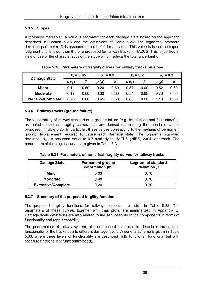
Fragility functions for transportation infrastructures
109
5.3.5 Slopes
A threshold median PGA value is estimated for each damage state based on the approach described in Section 5.2.8 and the definitions of Table 5.26. The lognormal standard deviation parameter, β, is assumed equal to 0.6 for all cases. This value is based on expert judgment and is lower than the one proposed for railway tracks in HAZUS. This is justified in view of use of the characteristics of the slope which reduce the total uncertainty.
Table 5.30 Parameters of fragility curves for railway tracks on slope
Damage State ky = 0.05 ky = 0.1 ky = 0.2 ky = 0.3
μ (g) β μ (g) β μ (g) β μ (g) β Minor 0.11 0.60 0.20 0.60 0.37 0.60 0.52 0.60
Moderate 0.17 0.60 0.30 0.60 0.54 0.60 0.78 0.60 Extensive/Complete 0.26 0.60 0.45 0.60 0.80 0.60 1.13 0.60
5.3.6 Railway tracks (ground failure)
The vulnerability of railway tracks due to ground failure (e.g. liquefaction and fault offset) is estimated based on fragility curves that are derived considering the threshold values proposed in Table 5.23. In particular, these values correspond to the medians of permanent ground displacement required to cause each damage state. The lognormal standard deviation, βtot, is assumed equal to 0.7 similarly to HAZUS (NIBS, 2004) approach. The parameters of the fragility curves are given in Table 5.31.
Table 5.31 Parameters of numerical fragility curves for railway tracks
Damage State Permanent ground deformation (m)
Lognormal standard deviation β
Minor 0.03 0.70 Moderate 0.08 0.70
Extensive/Complete 0.20 0.70
5.3.7 Summary of the proposed fragility functions
The proposed fragility functions for railway elements are listed in Table 5.32. The parameters of these curves, together with their plots, are summarized in Appendix C. Damage scale definitions are also related to the serviceability of the components in terms of functionality and repair capability.
The performance of railway system, at a component level, can be described through the functionality of the tracks due to different damage levels. A general scheme is given in Table 5.33, where three levels of functionality are described (fully functional, functional but with speed restrictions, not functional/closed).
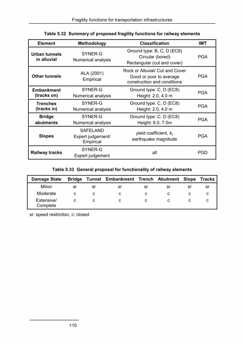
Fragility functions for transportation infrastructures
110
Table 5.32 Summary of proposed fragility functions for railway elements
Element Methodology Classification IMT
Urban tunnels in alluvial
SYNER-G Numerical analysis
Ground type: B, C, D (EC8) Circular (bored)
Rectangular (cut and cover) PGA
Other tunnels ALA (2001) Empirical
Rock or Alluvial/ Cut and Cover Good or poor to average
construction and conditions PGA
Embankment (tracks on)
SYNER-G Numerical analysis
Ground type: C, D (EC8) Height: 2.0, 4.0 m
PGA
Trenches (tracks in)
SYNER-G Numerical analysis
Ground type: C, D (EC8) Height: 2.0, 4.0 m PGA
Bridge abutments
SYNER-G Numerical analysis
Ground type: C, D (EC8) Height: 6.0, 7.5m
PGA
Slopes SAFELAND
Expert judgement/ Empirical
yield coefficient, ky
earthquake magnitude PGA
Railway tracks SYNER-G Expert judgement
all PGD
Table 5.33 General proposal for functionality of railway elements
Damage State Bridge Tunnel Embankment Trench Abutment Slope Tracks Minor sr sr sr sr sr sr sr
Moderate c c c c c c c Extensive/ Complete
c c c c c c c
sr: speed restriction, c: closed

Fragility functions for transportation infrastructures
111
5.4 HARBOUR ELEMENTS
5.4.1 Identification of main typologies
In a port system, the following elements are considered in SYNER-G:
o Waterfront structures;
o Cargo handling and storage components;
o Infrastructures;
o Buildings (sheds and warehouses, office buildings, maintenance buildings, passenger terminals, traffic control buildings);
o Utility systems (electric power system, water system, waste-water system, natural gas system, liquid fuel system, communications system, fire-fighting system);
o Transportation infrastructures (roadway system, railway system, bridges).
Important typological features of port components include:
o Waterfront structures. The basic typological parameters are their geometry, section type, construction material, foundation type, existence and type of anchorage. Types of backfill and foundation soil, along with the existence of rubble foundation are determinant factors of their seismic behaviour (Ichii, 2003). A more exhaustive typology is provided by Werner (1998) and PIANC (2001).
o Cargo handling and storage components. The basic typological parameter is the existence of anchorage. They could also be classified according to the cargo capacity and cargo type. When considering interactions between port components, their power supply type, foundation type and position are also important typological features. A more detailed typology is provided in Werner (1998).
The major typological parameters of infrastructure components (buildings, utility and transportation systems) are provided in the respective sections of the report. Specific features of infrastructures within facilities are given in Werner (1998).
5.4.2 Damage description
Earthquake effects on port elements can be grouped into two categories: ground shaking (expressed often in terms of peak ground acceleration); and ground failure such as liquefaction (expressed in terms of permanent ground deformations). A brief summary is given below for the port elements.
o Waterfront structures. Extensive seismic damage is usually attributed to the occurrence of soil liquefaction. Most failures are associated with outward sliding, deformation and tilting. For gravity-type quay walls, possible modes of seismic failure include (Kakderi et al., 2006): outward sliding, tilting, settlement, overturning and extensive tilting, collapse, apron pavement cracking, cracking with corresponding pavement settlement relative to wall. For the backfill materials, the failure modes are classified as: ground fracture and cracking of road surface, waterspouts from ground fissures and sand boils, settlement of backfill, differential ground settlement, and

Fragility functions for transportation infrastructures
112
lateral ground movement (lateral spreading). Block-type quay walls are also vulnerable to earthquake-induced sliding between layers of blocks. The principal failure mode of sheet-pile bulkheads has been insufficient anchor resistance. For pile-supported waterfront structures, possible failure modes are also related to earthquake induced sliding, buckling and/or yielding of piles (ATC-25).
o Cargo handling and storage components. When anchored to foundation rails, cranes are vulnerable to failure due to bending and ground shaking. In cases where relative movement or derailment is possible (anchorage failure or cranes in use), failure modes include: overturning due to liquefaction of underlying soil fills and/or the occurrence of differential settlements and bending type of failure due to ground detachment of a foundation member (PIANC, 2001). Disruption of cranes functionality may also be induced by settlement and/or horizontal movement of foundation rails due to liquefaction of subjacent soil layers. Modern jumbo cranes are expected to be severely damaged, or collapsed, in a major earthquake (Soderberg et al., 2009).
Fig. 5.14 Seaward movement of quay-wall during the 2003 Tokachi-Oki earthquake
(left), Turnover and extensive tilting of quay-walls during the 1995 Hyogo-ken Nanbu (Kobe) earthquake (right)
Different damage criteria have been proposed for the fragility analysis of port elements. The number of damage states is variable and in most cases is related to the description of the type and extent (level) of structural damage and the serviceability state. In empirical and expert judgment methods the extent of damage is described qualitatively (e.g. extent of settlements). In numerical methods the damage levels are defined based on the range of a specific damage index (e.g. normalized residual horizontal displacement). Damage criteria proposed by different studies are summarized in the next section.
5.4.3 State of the art fragility functions for harbour elements components
A review of existing fragility functions for port systems’ components is presented (i.e. waterfront structures, cargo handling and storage components, and port infrastructures). For port infrastructures (building structures, utility and transportation systems), there are no specific fragility functions (except for fuel facilities) and their vulnerability assessment is performed using available fragility functions for lifeline systems’ components. Table 5.34, Table 5.35 and
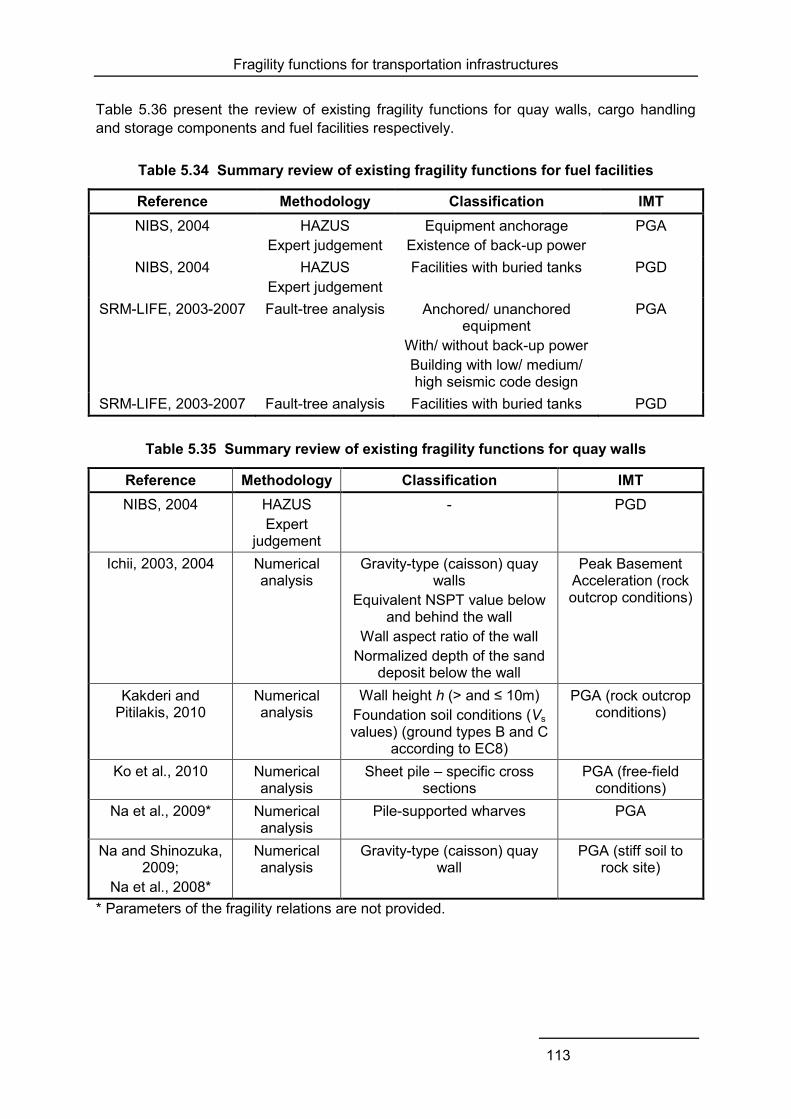
Fragility functions for transportation infrastructures
113
Table 5.36 present the review of existing fragility functions for quay walls, cargo handling and storage components and fuel facilities respectively.
Table 5.34 Summary review of existing fragility functions for fuel facilities
Reference Methodology Classification IMT NIBS, 2004 HAZUS
Expert judgement Equipment anchorage
Existence of back-up power PGA
NIBS, 2004 HAZUS Expert judgement
Facilities with buried tanks PGD
SRM-LIFE, 2003-2007 Fault-tree analysis Anchored/ unanchored equipment
With/ without back-up power Building with low/ medium/ high seismic code design
PGA
SRM-LIFE, 2003-2007 Fault-tree analysis Facilities with buried tanks PGD
Table 5.35 Summary review of existing fragility functions for quay walls
Reference Methodology Classification IMT NIBS, 2004 HAZUS
Expert judgement
- PGD
Ichii, 2003, 2004 Numerical analysis
Gravity-type (caisson) quay walls
Equivalent NSPT value below and behind the wall
Wall aspect ratio of the wall Normalized depth of the sand
deposit below the wall
Peak Basement Acceleration (rock outcrop conditions)
Kakderi and Pitilakis, 2010
Numerical analysis
Wall height h (> and ≤ 10m) Foundation soil conditions (Vs values) (ground types B and C
according to EC8)
PGA (rock outcrop conditions)
Ko et al., 2010 Numerical analysis
Sheet pile – specific cross sections
PGA (free-field conditions)
Na et al., 2009* Numerical analysis
Pile-supported wharves PGA
Na and Shinozuka, 2009;
Na et al., 2008*
Numerical analysis
Gravity-type (caisson) quay wall
PGA (stiff soil to rock site)
* Parameters of the fragility relations are not provided.

Fragility functions for transportation infrastructures
114
Table 5.36 Summary review of existing fragility functions for cargo handling and storage components
Reference Methodology Classification IMT NIBS, 2004
HAZUS, expert judgement
Stationary (anchored)/ rail-mounted (un-anchored)
PGA, PGD
5.4.4 Selection of appropriate fragility functions for European typologies
The evaluation and examination of the reliability of existing fragility curves has been performed based on the actual seismic performance of the quay walls of the city of Lefkas, which sustained significant deformations during the 2003 earthquake (Kakderi et al., 2006). The main conclusions of the study indicate that the vulnerability assessment and damage state distribution using the HAZUS (NIBS, 2004) relationships is rather compatible with the observed damages, while damages based on the vulnerability curves proposed from Ichii (2003) seem to be slightly overestimated. On the other hand, the application of the vulnerability functions by Ichii (2003) requires knowledge about the geotechnical and construction data. Their application is possible in case of lack of specific studies for the estimation of permanent ground deformations.
The previous validation studies refer only to the case of induced damages due to ground failure. When considering only the case of ground shaking without the occurrence of liquefaction phenomena, specific fragility functions need to be applied.
Based on the above, the fragility curves in HAZUS (NIBS, 2004) are proposed for the vulnerability assessment of quay walls for the case of ground failure. For the case of ground shaking, without considering the occurrence of liquefaction phenomena, the analytically derived fragility curves of Kakderi and Pitilakis (2010) are proposed. Other available analytical studies lack general applicability, as they refer to specific structures and/or parameters of the fragility relations are not provided.
For cargo handling and storage components, the only available fragility curves are those of HAZUS (NIBS, 2004) which are proposed here, while for fuel and communication facilities the fragility functions proposed in SRMLIFE (2003-2007) are the ones most applicable to the European typology. They are developed based on fault-tree analysis, using the fragility curves of Kappos et al. (2006a) for the building sub-components.
5.4.5 Summary of the proposed fragility functions
In Table 5.37 the proposed fragility functions for harbour elements are outlined. The parameters of these curves and the corresponding serviceability levels, together with their plots, are summarized in Appendix C. For buildings, electric power, water, waste-water, natural gas, fire-fighting, roadway/railway systems and bridges, see the respective sections.

Fragility functions for transportation infrastructures
115
Table 5.37 Summary of the proposed fragility functions for harbour elements
Element Methodology Classification IMT Waterfront structures
HAZUS Expert judgment
One class PGD
Waterfront structures
Kakderi and Pitilakis (2010)
Numerical analysis
Wall height h (> and ≤ 10m) Soil foundation conditions (Vs values) (ground types B and C
according to EC8)
PGA
Cargo handling and storage components
HAZUS Expert judgment
Stationary (anchored) and rail-mounted (un-anchored) cranes
PGA, PGD
Liquid fuel system
SRMLIFE (2003-2007) Fault-tree analysis
Anchored/ unanchored equipment With/ without back-up power
Building with low/ medium/ high seismic code design
PGA
Liquid fuel system
SRMLIFE (2003-2007) Fault-tree analysis
Facilities with buried tanks PGD
Communication system
SRMLIFE (2003-2007) Fault-tree analysis
Anchored components Low-rise/ mid-rise building
Low/ high seismic code design PGA


Fragility functions for critical facilities
117
6 Fragility functions for critical facilities
6.1 HEALTH-CARE FACILITIES
6.1.1 System components
Hospital facilities belong to the category of the so-called “complex-social” systems: complex because, from an engineering point of view, these systems are made of many components of different nature that jointly contribute to provide an output which is the medical services; social, because hospitals provide a fundamental assistance to citizens in every-day life and their function becomes of paramount importance in the case of a disaster. The system taxonomy for hospitals is illustrated in Fig. 6.1.
Fig. 6.1 System taxonomy of a hospital
At the core of the system there are the medical services, which consist of standardized procedures established to guarantee an adequate treatment of patients. The medical services are delivered to patients by a joint contribution of the three “active” components of the system:
o The facility (physical component) where the medical services are delivered. The physical component of a hospital system consists of structural elements and non-structural elements (architectural elements, basic contents and equipment). While the former are critical to preserve the life-safety of the building occupants, the latter are fundamental to preserve the hospital functionality.
o The operators, which are the doctors, nurses and in general whoever plays an active role in providing medical care.
o The organisation, which is responsible of setting up the adequate conditions so that the medical services can be delivered. In general, this is up to the hospital management through the development, the implementation and the supervision of the standardized procedures.
The environment includes all external influences to the functioning of a hospital system, which encompasses such diverse factors as cultural background and soil properties. It acts on all the “active” components both directly, through characteristics such as accessibility, soil
MedicalServices
Operators Organisation
Facilities
Patient in Patient out
Envinroment
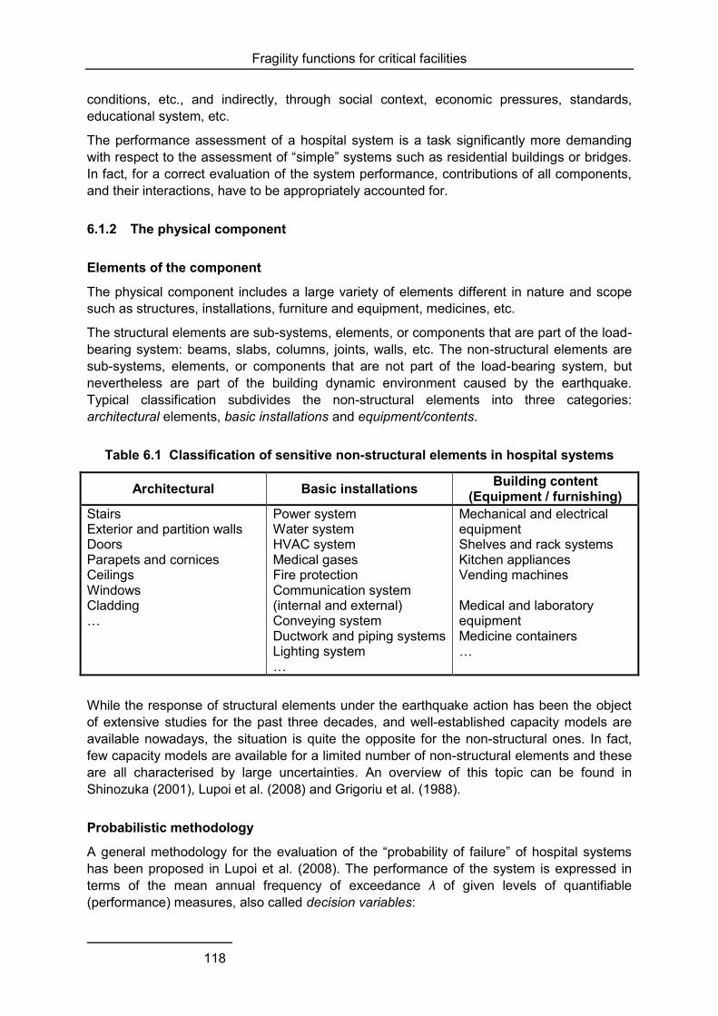
Fragility functions for critical facilities
118
conditions, etc., and indirectly, through social context, economic pressures, standards, educational system, etc.
The performance assessment of a hospital system is a task significantly more demanding with respect to the assessment of “simple” systems such as residential buildings or bridges. In fact, for a correct evaluation of the system performance, contributions of all components, and their interactions, have to be appropriately accounted for.
6.1.2 The physical component
Elements of the component
The physical component includes a large variety of elements different in nature and scope such as structures, installations, furniture and equipment, medicines, etc.
The structural elements are sub-systems, elements, or components that are part of the load-bearing system: beams, slabs, columns, joints, walls, etc. The non-structural elements are sub-systems, elements, or components that are not part of the load-bearing system, but nevertheless are part of the building dynamic environment caused by the earthquake. Typical classification subdivides the non-structural elements into three categories: architectural elements, basic installations and equipment/contents.
Table 6.1 Classification of sensitive non-structural elements in hospital systems
Architectural Basic installations Building content (Equipment / furnishing)
Stairs Exterior and partition walls Doors Parapets and cornices Ceilings Windows Cladding …
Power system Water system HVAC system Medical gases Fire protection Communication system (internal and external) Conveying system Ductwork and piping systems Lighting system …
Mechanical and electrical equipment Shelves and rack systems Kitchen appliances Vending machines Medical and laboratory equipment Medicine containers …
While the response of structural elements under the earthquake action has been the object of extensive studies for the past three decades, and well-established capacity models are available nowadays, the situation is quite the opposite for the non-structural ones. In fact, few capacity models are available for a limited number of non-structural elements and these are all characterised by large uncertainties. An overview of this topic can be found in Shinozuka (2001), Lupoi et al. (2008) and Grigoriu et al. (1988).
Probabilistic methodology
A general methodology for the evaluation of the “probability of failure” of hospital systems has been proposed in Lupoi et al. (2008). The performance of the system is expressed in terms of the mean annual frequency of exceedance λ of given levels of quantifiable (performance) measures, also called decision variables:
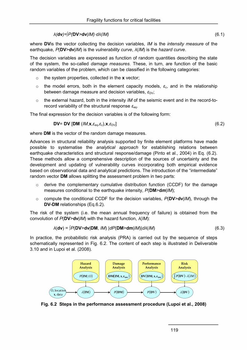
Fragility functions for critical facilities
119
λ(dv)=∫P(DV>dv|IM)⋅dλ(IM) (6.1)
where DVis the vector collecting the decision variables, IM is the intensity measure of the earthquake, P(DV>dv|IM) is the vulnerability curve, λ(IM) is the hazard curve.
The decision variables are expressed as function of random quantities describing the state of the system, the so-called damage measures. These, in turn, are function of the basic random variables of the problem, which can be classified in the following categories:
o the system properties, collected in the x vector;
o the model errors, both in the element capacity models, εc, and in the relationship between damage measure and decision variables, εDV;
o the external hazard, both in the intensity IM of the seismic event and in the record-to-record variability of the structural response εeq.
The final expression for the decision variables is of the following form:
DV= DV [DM (IM,x,εeq,εc),x,εDV] (6.2)
where DM is the vector of the random damage measures.
Advances in structural reliability analysis supported by finite element platforms have made possible to systematise the analytical approach for establishing relations between earthquake characteristics and structural response/damage (Pinto et al., 2004) in Eq. (6.2). These methods allow a comprehensive description of the sources of uncertainty and the development and updating of vulnerability curves incorporating both empirical evidence based on observational data and analytical predictions. The introduction of the “intermediate” random vector DM allows splitting the assessment problem in two parts:
o derive the complementary cumulative distribution function (CCDF) for the damage measures conditional to the earthquake intensity, P(DM>dm|IM);
o compute the conditional CCDF for the decision variables, P(DV>dv|IM), through the DV-DM relationships (Eq.6.2).
The risk of the system (i.e. the mean annual frequency of failure) is obtained from the convolution of P(DV>dv|IM) with the hazard function, λ(IM):
λ(dv) = ∫P(DV>dv|DM, IM) |dP(DM>dm|IM)|dλ(IM) (6.3)
In practice, the probabilistic risk analysis (PRA) is carried out by the sequence of steps schematically represented in Fig. 6.2. The content of each step is illustrated in Deliverable 3.10 and in Lupoi et al. (2008).
Fig. 6.2 Steps in the performance assessment procedure (Lupoi et al., 2008)
PerformanceAnalysis
DMεxDMDV ,,
DamageAnalysis
DMεxIMDM ,,
HazardAnalysis
OP |IM
IM DMP DVPlocation,O
data,x
RiskAnalysis
DV
IMP DV
Fragility functions for critical facilities
120
The accuracy of a PRA resides, for a good part, in a realistic and comprehensive description of all the important sources of uncertainty. The uncertainties that affect the reliability of the physical components can be broadly classified as follows:
o those related to the external hazard;
o those related to the evaluation of the structural response, i.e. the finite element model, the type of analysis (static or dynamic, linear or non-linear, type of non-linearity, soil-structure interaction), etc.;
o those related to the knowledge of system properties, such as size, weight, stiffness, strength, characteristics of the interface between the element and the structure;
o those related to the modelling of the capacities of both structural and non-structural vulnerable elements;
o those related to performances, such as the definition of damage levels and of the consequences associated to exceeding any limit-state.
Capacity models for assessment
Capacity and demand have to be expressed in terms of local response quantities well-correlated to damage to adequately represent the actual state of an element. The definition of models capable of describing elements capacity is a major task in the overall assessment procedure. In fact, “capacity models developed and used for assessment purposes bear a conceptual difference with respect to those used in design. The latter generally tend to be simple to use and approximated in a conservative way, which makes them unsuitable for a consistent evaluation of risk. Risk assessment requires explicit consideration of all relevant uncertainties, aleatoric and epistemic, and probabilistic models that are unbiased. A conservative model does not comply with this requirement” (LESSLOSS, 2005).
The definition of a capacity model is generally based on one of the following approaches: empirical, theoretical or judgment-based.
Empirical approaches are based on the statistical analysis of the performance of the element during past earthquakes. These data may derive from instrumented and non-instrumented buildings. Instrumented buildings are a potentially excellent source of information not yet adequately exploited. Non-instrumented buildings represent a less reliable, but more readily available source of information: a damage-motion relation can be obtained relating data on damage from detailed damage inspections with data on motion from structural analysis. Empirical approaches include also experimental tests, one of the most reliable sources of data to study the damage as a result of applied loads, since everything in an experiment is monitored closely. Unfortunately the results and the procedures applied in the tests are not always well-documented.
Theoretical approaches are based on analytical simulations (static and dynamic analysis) of a mechanical model of the element.
Judgment-based approaches represent the opinion of experts.
Preference for a given approach depends on circumstances. In practice, the information for the development of capacity models has been usually obtained empirically, but it is recognized the need for combining the three approaches to achieve a good capacity model.

Fragility functions for critical facilities
121
RC structural elements
Failure mechanisms in RC structures may be localised at the elements level (beam, columns and joints) or at a global scale for the formation of a mechanism (more elements involved).
Local response parameters can be (a) force quantities, such as shear failure (force mechanisms), in evaluation of the state of the element with respect to the activation of force-controlled failure mechanisms, or (b) displacement/deformation quantities, such as inter-storey drift ratios or chord-rotations, in evaluation of the element damage state with respect to displacement-related mechanisms.
The global failure of the RC structure typically occurs due to the formation of a weak-storey mechanism. The generic fault tree for RC structures is provided in Deliverable 3.10 of SYNER-G.
A vast literature is available on capacity models for RC structural elements. However, the available capacity formulas are generally based on relatively weak mechanical basis, integrated with empirical knowledge. In the proposed method, the capacity terms are expressed in the multiplicative format Ci(x, εC) = i(x)εCi, where i(x) is the value obtained by semi-empirical formulas available in the literature, and εCi is a model-error term accounting for scatter and, when necessary, for bias as well. The type of distribution of εCi is based on expert judgment.
The recommended models for the estimation of members’ shear strength, deformation and drift capacity are described in the Deliverable 3.10 of SYNER-G.
Non-structural elements
The selection of the local response parameter for a non-structural element depends on the following loading mechanism governing the response:
o local acceleration, which may cause the element sliding or overturning;
o structural deformation;
o relative movements between adjacent or connected structures.
In general, a restrained non-structural element is drift sensitive, while a free non-structural element is acceleration sensitive. The differential-displacement sensitive elements are those which provide a continuous link across a separation joint or between two different structures.
Elements that hang from floor slabs and beams, such as most mechanical and electrical components, ceilings and contents, are examples of acceleration sensitive elements; glazing, doors and partition walls, which are tightly locked into the structure, are examples of structural deformation sensitive elements. Some components are sensitive to both inter-storey drift and peak floor acceleration. Elevators have rails, doors and other components that are damaged primarily by inter-storey drift ratios, while others, such as the motor and counterweights, are damaged as a result of floor accelerations.
Items that are connected to objects with independent movement, i.e. utilities extended across the separation joints, should be capable of providing functional continuity and therefore are sensitive to differential displacements.
Based on the above considerations, non-structural elements are usually classified as: acceleration-sensitive, deformation (drift)-sensitive or differential-displacement sensitive.
Fragility functions for critical facilities
122
The definition of capacity models for non-structural elements is not straightforward. In fact, although the general working principles are the same for all elements, each one has its own unique adaptation that makes it different from the others. For example, the interface between the elements and the structure can take different forms: elements can be fixed to the floor, supported by a layer of interposed material intended to isolate them from the floor motion, or placed securely in a rack fixed to the floor and wall, etc. Since an accurate modelling for all non-structural elements is not practical, the following approach is adopted:
o generic capacity models are employed for classes of “non-critical” elements;
o specific capacity models are developed for critical elements.
The fragility curves for these models are provided in appendix D.
Non-structural elements: Architectural
The architectural elements are typically built-in non-structural components that form part of the building. Those that have jeopardised the functionality of several hospitals in past earthquakes are:
o interior and exterior walls;
o ceilings;
o windows, glasses and doors.
Walls are made of masonry or other materials and are typically stiffer and more brittle than the structural frame; therefore, they tend to develop cracks when the building is subjected to earthquake shaking. Usually, the crack growth is initiated at the corner of an opening in the wall. The failure of either interior or exterior walls can be attributed to (a) excessive flexural out-of-plane stresses induced by floor accelerations or (b) excessive in-plane shear stresses induced by inter-storey drifts imposed on the building structure. Studies on the seismic performance of walls have been performed, among others, by Freeman (1977), Rihal (1982) and Cohen (1995).
Ceilings are non-structural elements that are sensitive to both deformation and acceleration. The deformation of the floor slabs can cause horizontal distortion and the deformation of the main structure, leading to possible loss of support and fall of the ceiling. Gates and McGavin (1998) point out the interaction between the ceiling system and both the fire sprinkler system and the lighting fixtures. References to this type of non-structural elements are, among others, Eidenger and Goettel (1998), Yao (2000), Badillo et al. (2003) and Gann et al. (2005).
Elements that are attached to the structure or to non-structural walls, such as doors, windows, glazing, can twist and buckle when they are subjected to large deformations. Most often deformation of the structural frame can jam the element (as in the case of doors) or cause failure (as in the case of glazing) due to the inadequate edge clearance around the item (door, glazing, windows, etc.). The performance of glass doors, windows and glazing during earthquakes is highly dependent on the deformation capacity provided to the brittle material with respect to its supporting frame. Failure of this kind of elements causes not only a problem for the functionality but could also produce injuries. Studies on this category have been conducted, among others, by Bouwkamp and Meehan (1960), Nakata et al. (1984) and Behr and Worrell (1998).
The generic fault tree for architectural elements is provided in Deliverable 3.10 of SYNER-G.
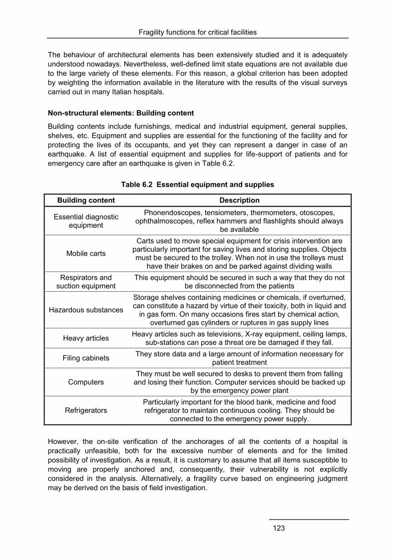
Fragility functions for critical facilities
123
The behaviour of architectural elements has been extensively studied and it is adequately understood nowadays. Nevertheless, well-defined limit state equations are not available due to the large variety of these elements. For this reason, a global criterion has been adopted by weighting the information available in the literature with the results of the visual surveys carried out in many Italian hospitals.
Non-structural elements: Building content
Building contents include furnishings, medical and industrial equipment, general supplies, shelves, etc. Equipment and supplies are essential for the functioning of the facility and for protecting the lives of its occupants, and yet they can represent a danger in case of an earthquake. A list of essential equipment and supplies for life-support of patients and for emergency care after an earthquake is given in Table 6.2.
Table 6.2 Essential equipment and supplies
Building content Description
Essential diagnostic equipment
Phonendoscopes, tensiometers, thermometers, otoscopes, ophthalmoscopes, reflex hammers and flashlights should always
be available
Mobile carts
Carts used to move special equipment for crisis intervention are particularly important for saving lives and storing supplies. Objects must be secured to the trolley. When not in use the trolleys must
have their brakes on and be parked against dividing walls Respirators and
suction equipment This equipment should be secured in such a way that they do not
be disconnected from the patients
Hazardous substances
Storage shelves containing medicines or chemicals, if overturned, can constitute a hazard by virtue of their toxicity, both in liquid and
in gas form. On many occasions fires start by chemical action, overturned gas cylinders or ruptures in gas supply lines
Heavy articles Heavy articles such as televisions, X-ray equipment, ceiling lamps, sub-stations can pose a threat ore be damaged if they fall.
Filing cabinets They store data and a large amount of information necessary for patient treatment
Computers They must be well secured to desks to prevent them from falling
and losing their function. Computer services should be backed up by the emergency power plant
Refrigerators Particularly important for the blood bank, medicine and food refrigerator to maintain continuous cooling. They should be
connected to the emergency power supply.
However, the on-site verification of the anchorages of all the contents of a hospital is practically unfeasible, both for the excessive number of elements and for the limited possibility of investigation. As a result, it is customary to assume that all items susceptible to moving are properly anchored and, consequently, their vulnerability is not explicitly considered in the analysis. Alternatively, a fragility curve based on engineering judgment may be derived on the basis of field investigation.

Fragility functions for critical facilities
124
Non-structural elements: Basic installations
Across all occupancies, including essential facilities, the most disruptive kind of non-structural damage is the breakage of water lines inside buildings, including fire sprinklers, domestic water and chilled-water systems. Leaked water can spread quickly throughout a building.
Second in significance is failure of emergency power systems. The power outage is usually so extensive that reliable backup power is necessary for essential facilities to operate. Others frequently damaged installations, among those essential for the functioning of hospitals, are the conveying and the medical gas systems.
Each of such systems can be subdivided in two main components:
a) Generation: it can be provided by an internal or an external source. However, in an emergency situation, all the essential systems have to be complemented with an internal source. Examples of internal sources are electrical generator, water tank, gas tank. Their typical mode of failure is the damage of anchorages.
b) Distribution: it includes pipes for water, for wastewater, for fuel, for gas and electrical conduits (lines) that run underground or above grade, inside and outside the building. Damage to above-ground transmission lines typically occurs along unsupported line sections when lines crack, leak, or fail. Damage to underground transmission lines usually occurs in areas of soil failure where the line sections cannot accommodate soil movements or differential settlements. Damage can also occur when other equipment falls over the line, or if a piece of equipment to which the line is connected is damaged. Lines that run across a seismic joint without an expansion joint may suffer damage to their connections or get torn apart. It is noted that electric power is necessary for the proper functioning of the distribution lines.
The generic fault tree for a basic installation is provided in Deliverable 3.10 of SYNER-G.
Medical gas
The medical gas system of a hospital typically consists of tanks and cylinders of the medical gases (oxygen, nitrogen, etc.), the distribution lines (pipes) and several other pieces of equipment necessary to the normal functioning such as, for example, electric pumps. The cylinders and the auxiliary equipments are usually located in a large room at the base floor of the building. The generic fault tree for the medical gas system is provided in Deliverable 3.10 of SYNER-G.
Power system
The power system of an hospital buildings is typically composed of:
o MV-LV (Medium Voltage - Low Voltage) transformation station;
o Uninterruptible Power System (UPS);
o Emergency Power Generator (EPG);
o transmission lines;
o distribution stations.
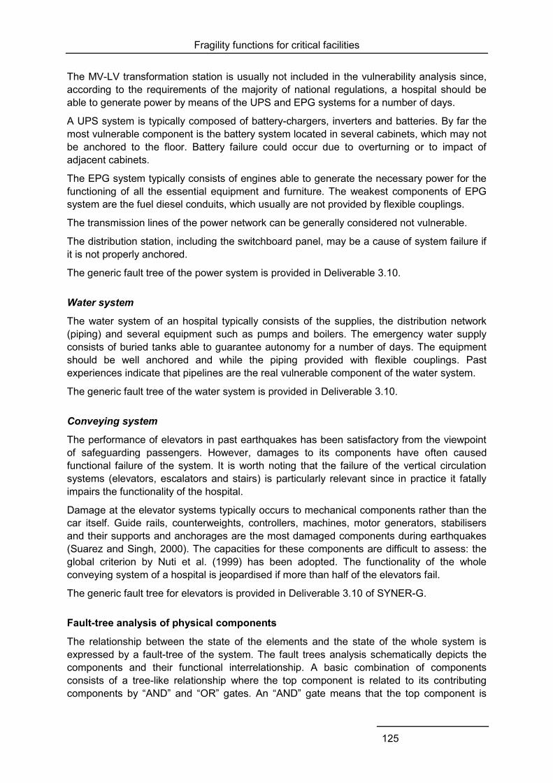
Fragility functions for critical facilities
125
The MV-LV transformation station is usually not included in the vulnerability analysis since, according to the requirements of the majority of national regulations, a hospital should be able to generate power by means of the UPS and EPG systems for a number of days.
A UPS system is typically composed of battery-chargers, inverters and batteries. By far the most vulnerable component is the battery system located in several cabinets, which may not be anchored to the floor. Battery failure could occur due to overturning or to impact of adjacent cabinets.
The EPG system typically consists of engines able to generate the necessary power for the functioning of all the essential equipment and furniture. The weakest components of EPG system are the fuel diesel conduits, which usually are not provided by flexible couplings.
The transmission lines of the power network can be generally considered not vulnerable.
The distribution station, including the switchboard panel, may be a cause of system failure if it is not properly anchored.
The generic fault tree of the power system is provided in Deliverable 3.10.
Water system
The water system of an hospital typically consists of the supplies, the distribution network (piping) and several equipment such as pumps and boilers. The emergency water supply consists of buried tanks able to guarantee autonomy for a number of days. The equipment should be well anchored and while the piping provided with flexible couplings. Past experiences indicate that pipelines are the real vulnerable component of the water system.
The generic fault tree of the water system is provided in Deliverable 3.10.
Conveying system
The performance of elevators in past earthquakes has been satisfactory from the viewpoint of safeguarding passengers. However, damages to its components have often caused functional failure of the system. It is worth noting that the failure of the vertical circulation systems (elevators, escalators and stairs) is particularly relevant since in practice it fatally impairs the functionality of the hospital.
Damage at the elevator systems typically occurs to mechanical components rather than the car itself. Guide rails, counterweights, controllers, machines, motor generators, stabilisers and their supports and anchorages are the most damaged components during earthquakes (Suarez and Singh, 2000). The capacities for these components are difficult to assess: the global criterion by Nuti et al. (1999) has been adopted. The functionality of the whole conveying system of a hospital is jeopardised if more than half of the elevators fail.
The generic fault tree for elevators is provided in Deliverable 3.10 of SYNER-G.
Fault-tree analysis of physical components
The relationship between the state of the elements and the state of the whole system is expressed by a fault-tree of the system. The fault trees analysis schematically depicts the components and their functional interrelationship. A basic combination of components consists of a tree-like relationship where the top component is related to its contributing components by “AND” and “OR” gates. An “AND” gate means that the top component is
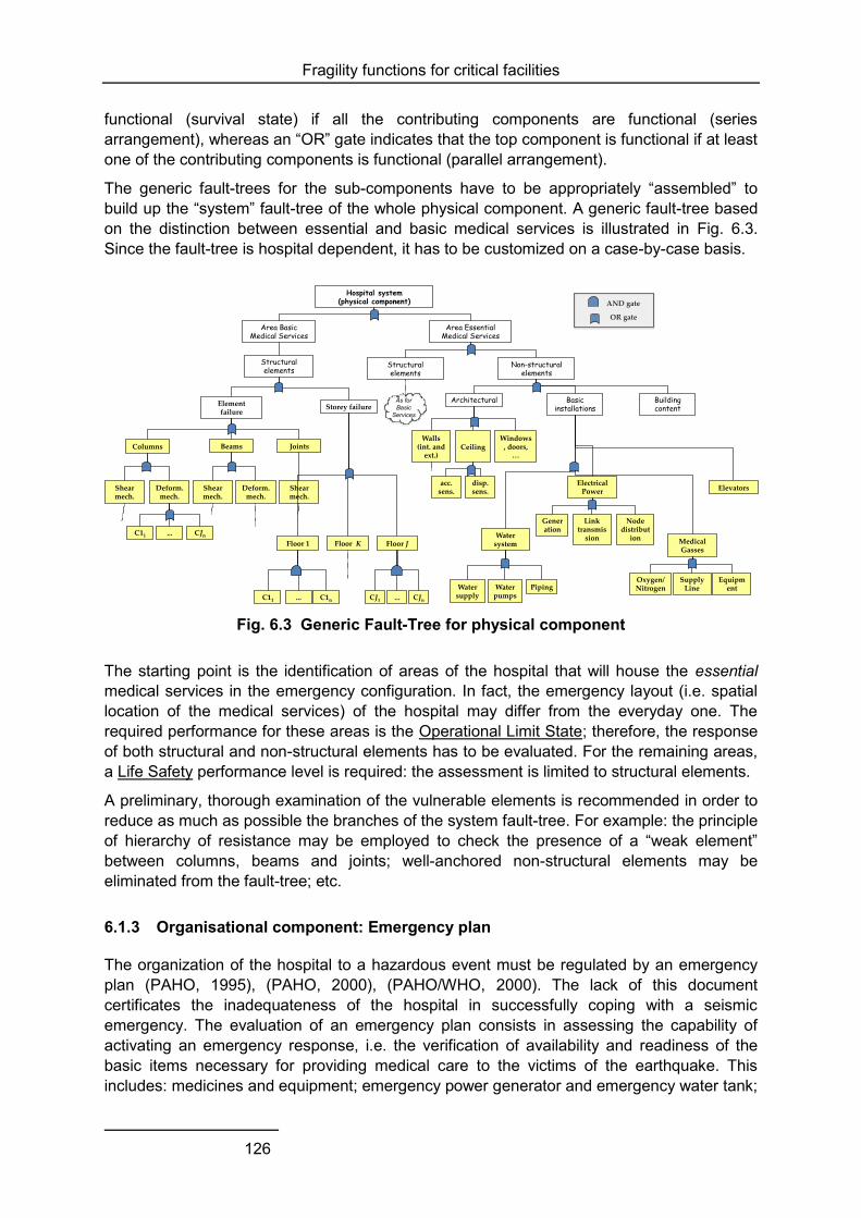
Fragility functions for critical facilities
126
functional (survival state) if all the contributing components are functional (series arrangement), whereas an “OR” gate indicates that the top component is functional if at least one of the contributing components is functional (parallel arrangement).
The generic fault-trees for the sub-components have to be appropriately “assembled” to build up the “system” fault-tree of the whole physical component. A generic fault-tree based on the distinction between essential and basic medical services is illustrated in Fig. 6.3. Since the fault-tree is hospital dependent, it has to be customized on a case-by-case basis.
Fig. 6.3 Generic Fault-Tree for physical component
The starting point is the identification of areas of the hospital that will house the essential medical services in the emergency configuration. In fact, the emergency layout (i.e. spatial location of the medical services) of the hospital may differ from the everyday one. The required performance for these areas is the Operational Limit State; therefore, the response of both structural and non-structural elements has to be evaluated. For the remaining areas, a Life Safety performance level is required: the assessment is limited to structural elements.
A preliminary, thorough examination of the vulnerable elements is recommended in order to reduce as much as possible the branches of the system fault-tree. For example: the principle of hierarchy of resistance may be employed to check the presence of a “weak element” between columns, beams and joints; well-anchored non-structural elements may be eliminated from the fault-tree; etc.
6.1.3 Organisational component: Emergency plan
The organization of the hospital to a hazardous event must be regulated by an emergency plan (PAHO, 1995), (PAHO, 2000), (PAHO/WHO, 2000). The lack of this document certificates the inadequateness of the hospital in successfully coping with a seismic emergency. The evaluation of an emergency plan consists in assessing the capability of activating an emergency response, i.e. the verification of availability and readiness of the basic items necessary for providing medical care to the victims of the earthquake. This includes: medicines and equipment; emergency power generator and emergency water tank;
Area Basic Medical Services
Structural elements
Area Essential Medical Services
Structural elements
Non-structural elements
Hospital system (physical component)
Basic installations
Building content
Architectural
Walls (int. and
ext.)
acc. sens.
disp. sens.
CeilingWindows
, doors, …
Element failure
Storey failure
Shear mech.
Deform. mech.
Columns
Shear mech.
Deform. mech.
Beams
Shear mech.
Joints
C11 ... C1n
Floor 1 Floor K
CJ1 ... CJn
Floor J
C11 ... CJn Water system
Water supply
Water pumps
Piping
Electrical Power
Generation
Link transmis
sion
Node distribut
ion Medical Gasses
Oxygen/Nitrogen
Supply Line
Equipment
Elevators
As for
Basic
Services
AND gate
OR gate

Fragility functions for critical facilities
127
portable equipment; emergency communication system; emergency layout of the medical services, with the essential medical services located in areas that satisfy the operational performance limit state. Under an emergency condition, the available resources may be distributed among indoor and outdoor areas. The procedures to be activated and who is responsible of what have to be explicitly stated in the emergency plan.
6.1.4 Human component: Operators
The evaluation of the Human component involves the assessment of:
a) skill of operators;
b) availability of operators.
The skill is evaluated by expert opinion on the basis of questionnaires, age, experience and expertise, training and preparedness for emergency response.
The availability of medical personnel depends on the time of earthquake occurrence. It is generally acknowledged that, in the European context, the availability of operators is less critical than that of physical resources. However, it is advisable to verify this assumption.
The number of operators for the critical medical services is examined under the most severe condition, i.e. at night-time. The available human resources are compared, for different time-scenarios, with what actually is needed for the functioning at full capacity of all the critical medical services (assuming full-functionality of the physical components of the hospital, i.e. no damage to structural and non structural elements).
Operators not in service but available at short notice (e.g. ½ hour) can be accounted for. In addition, operators may be transferred from non-critical to critical areas under emergency conditions (for example, from hotel services to operating theatres).
6.1.5 Environment component
The analysis of the environment component leads to the evaluation of the number of victims that need to be hospitalised.
Type 1 elements – Severity index
The epidemiology of the injuries provides fundamental information for estimating the type and the amount of the resources needed to treat casualties. A patient’s condition is classified according to the triage colour-code, where a red tag identifies the patients who require immediate care, the yellow tag is used for those who require delayed care, the green tag is for those who need minimal care, and the blue and black tag indicate the deaths.
The medical severity of an event as a function of the patients’ conditions is commonly assessed by means of two severity indexes: S1 which represents the medical severity of the event, S2which is a measure of the severity of the injuries caused by the event. For the same number of casualties, the larger is the value of S2the greater is the amount of medical resources that are needed to treat the victims. According to data from past earthquakes, the value of S1 is between 0.1 and 0.5, while that of S2 is between 0.15 and 0.6.

Fragility functions for critical facilities
128
Type 2 elements – Casualty model
Casualty models provide estimates of the sum of the “severely injured” people (i.e. those requiring hospital treatment) and of the deaths. The lightly injured people are not considered. The engineering-based earthquake casualty models provide a rapid estimation of the earthquake impact on population for the purposes of response planning and mitigation. They have typically been developed by engineers from limited, anecdotal, historical data (not from epidemiological studies, nor involving health related researchers).
The casualty model proposed by Coburn and Spence (1992) and simplified by Nuti and Vanzi (1998) can be employed for the European context. The number of casualties is expressed as a percentage of the population through the following relationship:
C(IM) = k(IM− IMmin)4 (6.4)
where IM is the intensity measure of the seismic event, k and IMmin are the model parameters which take into account both the vulnerability of the building stock and the occupancy rate. These parameters have to be calibrated as a function of the specific environment conditions. According to the model, for a given earthquake scenario, the extent of building damage in the affected area is estimated by means of appropriate vulnerability functions. These models are affected by large uncertainties; hence, a model error term has been introduced in Lupoi et al. (2008).
The total number of casualties, given as the sum of red-tagged, yellow-tagged, and black-tagged victims, is given by the following expression:
Ncas(IM) = C(IM)casNpop (6.5)
where C(IM) is the number of victims as percentage of the population according to Eq. (6.4), Npop is the population in the area affected and cas is the model error term. The hospital tributary area can be evaluated by assigning each municipality to the closest main hospital, i.e. among those able to provide adequate medical assistance to serious casualties.
Hospital treatment demand
The Hospital Treatment Demand, HTD, provides an estimate of the number of people that require surgical attention. It is therefore related to the number of casualties and to the epidemiology of the event. The HTD index may be evaluated by the expression:
HTD = ζNT1+T2 (6.6)
where NT1+T2 is the number of red- and yellow-tagged patients and ζ is a factor accounting for the proportion of patients that require surgical attention. The value of the factor ζ may vary between⅓ and ½ according to experience; the actual value may be defined on case-by-case basis by expert opinion. The value of NT1+T2 can be derived from combining expression of the casualty model (eq. 6.5) with those of the severity indices S1 and S2 given in Eq. (6.1) and Eq. (6.2). The final expression for HTD derived in Lupoi et al. (2008) is:
HTD = ζ NT1+T2 = ζ S2 / (S1 + S1S2 + S2) NCas = (
(6.7) = ζ S2/(S1+ S1S2+ S2) C(IM) εCasNpop
Fragility functions for critical facilities
129
6.1.6 Performance of hospitals under emergency conditions: Hospital Treatment Capacity
The seismic performance of a hospital system is evaluated in terms of the capability to accommodate a sudden incoming flow of patients requiring hospitalisation. The corresponding performance measure is the Hospital Treatment Capacity (HTC) index, defined as the number of patients with serious injuries that the hospital can treat in one hour. The evaluation of the HTC index is affected by large uncertainties since it is a function of several factors of difficult quantification, ranging from the medical conditions of the patients to the amount of resources available.
The functional analysis of an hospital system under emergency conditions yielded the following major conclusions (see SYNER-G’s Deliverable D2.8):
1. the hospital treatment capacity (HTC) can be quantitatively measured by the number of functioning operating theatres, which represent the bottleneck of the health-care system after a mass-casualty event that produces trauma victims;
2. the influence of the organizational and human components on the HTC can be estimated only empirically on the basis of expert judgment;
3. the relationship between the damage state of the physical component and the HTC is (analytically) evaluated by means of engineering-based methods;
4. the expression for the HTC index is the following:
HTC = ΑΒΓ1Γ2 / tm (6.8)
where:
o Α accounts for the efficiency of the emergency plan (organizational component);
o Β accounts for the quality, training and preparation of the operators (human component);
o Γ1 is the number of operating theatres which remain operative after the hazardous event;
o Γ2 is a Boolean function equal to 1 if the system “survives” and to 0 otherwise;
o tm is the mean duration of a surgical operation (measured in hours).
The survival condition for the hospital system is defined in terms of medical services available after the seismic event (Lupoi et al., 2008). A distinction is made between essential and basic medical services. The first ones are those necessary to provide adequate care in emergency condition, both to the earthquake seriously/critically injured victims and to the in-patients of the hospital. Typically these are:
o emergency department;
o operating theatres;
o intensive care unit;
o diagnostics;
o blood bank;
o haemodialysis;

Fragility functions for critical facilities
130
o urology;
o neonatology;
o gynaecology/obstetrics;
o paediatrics;
o laboratory;
o pharmacy.
The essential medical services have to stay operational after the event. The basic medical services are all the others.
The performance requirements for the system are conventionally set as follows:
a) the essential medical services have to remain operative;
b) the safeguard of human life has to be guaranteed for the basic medical services.
If the above requirements are both meet, the “survival condition” is satisfied and Γ2 = 1; otherwise, Γ2 = 0. Condition (a) depends on the response of both structural and non-structural elements of the building portion where essential medical services are housed; condition (b) depends on the response of structural elements only.
The fault-tree technique is employed to establish the relationship between the state of the elements and the state of the system. If the system survives (Γ2 = 1), the hospital resources are measured in terms of the functioning operating theatres, Γ1. The derivation of the vulnerability curve forΓ1 is carried out as illustrated in a previous section: a technique based on detailed structural analysis is employed since the categorization of hospital systems is practically impossible because the layout of the medical services is totally facility-dependent, making each hospital a “prototype”. In addition, the employment of a probabilistic approach is an almost inevitable choice due to the large uncertainties characterising most of the quantities that contribute to the system response.
The evaluation of the emergency plan results in assigning a value to the α-factor in the HTC index, Eq. (6.8). At the current state of development, this is done by engineering judgment. Typical value may range from 0.5, for very poor emergency plan, up to 1 for an excellent and complete one.
The evaluation of the skill and of the availability of the operators results in assigning a value to the Β-factor in the HTC index, Eq. (6.8). At the current state of development, this is done by engineering judgment. Typical value may range from 0.5, for poorly trained and understaffed operators, up to 1 for well-trained and adequately-staffed ones.
6.1.7 Summary of seismic risk analysis of hospital system
A hospital system is made of five components: human, organizational, physical, environmental and medical services. The medical services that have to remain operative after the seismic event in order to guarantee the adequate treatment of patients and victims are classified as essential medical services.
The seismic risk for an hospital system is measured by the comparisons between treatment demand and capacity:
HTD(IM) = ζS2 / (S1 + S1S2 + S2) C(IM) εcas Npop (6.9)
Fragility functions for critical facilities
131
HTC(IM) = ΑΒΓ1(IM) Γ2(IM) / tm (6.10)
The analysis of the human, the organizational, the environment and the medical services components consists in:
o verifying that the hospital is provided of all the essential medical services;
o assessing the quality of the emergency plan;
o verifying the existence of adequate resources to put into effect the emergency plan;
o assessing the quality of the human component and the availability of the operators to put in practice the emergency plan;
o examining the environment where the hospital is located that affects the number and the typology of victims.
The following data/information are derived:
1. estimates of the coefficients Α and Β in Eq. (6.10);
2. identification of the hospital areas where the essential medical services are housed;
3. fault-tree of the hospital system and fragilities for all the relevant elements at risk;
4. estimate of the casualty model parameters C(IM) and of the severity indexes of the event, S1 and S2in Eq. (6.9).
The numerical analysis of the physical component is carried out by a probabilistic procedure. It provides the number of functioning operating theatres, Γ1, and the system-survival Boolean function, Γ2, in Eq. (6.10). The “survival condition” of the physical component is expressed as a function of the performance of the medical services, making a distinction between the essential medical services and basic medical services (all the others): the operational performance level is required for the former, a life-safety performance level for the latter. The fault-tree technique is employed for the determination of the state of the system as a function of the state of its elements.

Fragility functions for critical facilities
132
6.2 FIRE-FIGHTING SYSTEMS
Fire is a common consequence of large earthquakes in urban and industrial areas. Fire-fighting activities can be prevented due to damages in the water or other (e.g. roadway) networks after large earthquakes. On the other hand, fire following earthquake is an extremely variable phenomenon, due to variability in the number of ignitions and in the extent of fire-spread from each ignition.
The fire-fighting system plays a major role in the management of crisis situations. It comprises not only the fire stations, pipeline network and fire faucets (either separate or dependent on the water supply system), but also a whole crisis management system (special units, fire fighters, etc).
6.2.1 Identification of main typologies
Usually fire-fighting system is part of a water system consisting of the same pipelines and storage tanks. In the case it is a separate network, it is usual that the storage tanks are made of steel, and the pipes are made of PVC. It is more common to find separate fire-fighting systems in small/confined areas with known needs, such as harbours, airports or hospitals and not in large urban areas.
For fire-fighting buildings the typological categories proposed in Section 3 can be used, while for the other elements the typologies described in water supply system can be applied.
6.2.2 Damage description
In the majority of cases, fire fighting needs of urban areas are covered by the water supply system. There are only very few references of separate fire-fighting systems, as well as reporting of incurred seismic damages. In general, the assessment of vulnerability and seismic losses to fire-fighting systems could be performed according to what is mentioned for water and waste-water system elements. For fire stations the methodologies proposed for RC and masonry building types in Europe could be used.
6.2.3 Fragility functions for fire-fighting systems
The available fragility functions for fire-fighting systems’ elements (pipes, storage tanks, pumping station, fire-station buildings)are described in previous sections (e.g. water and waste-water network, buildings). The functionality of fire-faucets can be estimated taking into account the connectivity with water system failures.
For pipes, storage tanks and pumping stations the proposed curves are the ones for water and waste-water systems elements. For fire-station buildings, the curves proposed for RC and masonry building types in Europe could be used.
It is noted that the fragility of fire-fighting system is closely connected with the possible fires just after the earthquake. The interaction between the road closures and the serviceability of water network with the fire-fighting system (if it is not separate from water system) is also essential.

Conclusions - Final remarks
133
7 Conclusions - Final remarks
7.1 METHODS FOR DERIVING FRAGILITY FUNCTIONS
The overall objective of SYNER-G in regards to fragility functions of elements at risk is to propose the most appropriate functions for the construction typologies in Europe. To this end, fragility curves from literature were collected, reviewed and, where possible, validated against observed damage, and harmonised. In some cases, the functions were modified and adapted, while in other cases, new curves were developed. The fragility functions are proposed for buildings, lifelines, transportation infrastructures and critical facilities.
Different approaches can be used to define the fragility curves. Empirical curves are specific to a particular region, while judgmental ones depend on the experience of the individual experts consulted. Analytical and hybrid approaches result in reduced bias and are becoming ever more attractive. Whatever the approach, choices must be made regarding the damage states, damage measures and their threshold values and the intensity measure. A wide range of options is available in the literature and only general recommendations for a choice based on effectiveness, efficiency, sufficiency, robustness and computability may be put forward. In principle, the use of a particular damage or intensity measure should be guided by the extent to which it corresponds to damage, but in practice it is related to the approach followed for the derivation of fragility curves.
7.2 FRAGILITY FUNCTIONS FOR REINFORCED CONCRETE AND MASONRY BUILDINGS
The review of existing fragility curves for buildings shows a variety of methodologies, damage states, damage and intensity measures. It also becomes clear that existing taxonomies could leave out a large number of characteristics that could be used to distinguish the seismic performance of buildings. Hence, a modular classification scheme was developed. This collapsible and expandable scheme gives the flexibility to describe a building with as much information as can be collected, and allows one to expand the taxonomy when more detailed information is available, for example, by adding new categories or sub-categories so as to describe all types of buildings.
The main outcome of the project is a set of fragility functions for the most important typologies in Europe, which are stored into the Fragility Function Manager. This dynamic tool was used for the harmonisation of the fragility curves and for the estimation of the associated uncertainty in their mean and standard deviation values. For simplicity, fragility curves were harmonised for the yielding and ultimate damage states, as it is difficult to compare the functions for the intermediate ones.
New fragility curves were developed for RC frame and wall-frame buildings designed to Eurocode 2 alone or for the three ductility classes of Eurocode 8. The curves were established point-by-point, from the probability that the (random variable) demand for given intensity measure exceeds the (random variable) capacity and consider shear failures, which

Conclusions - Final remarks
134
are normally ignored in analytical fragility studies. New fragility curves, accounting for out-of-plane failure and behaviour, were developed for stone masonry buildings.
A further contribution of SYNER-G is towards the quantification of the epistemic uncertainty in fragility functions for buildings. A methodology was developed and implemented in a software tool that can be used for other elements at risk.
7.3 FRAGILITY FUNCTIONS FOR UTILITY NETWORKS
A modern electric power network (EPN) is a complex interconnected system designed to generate, transform and transfer electric energy from generating units to various locations. Based on the review of the main recent works on fragility functions of EPN components, standard damage scales for micro- and macro-components were proposed together with the most appropriate fragility functions for the components that are of interest in SYNER-G.
The existing fragility curves for pipelines, storage tanks and support facilities within natural gas and oil networks were collected and reviewed. Existing fragility curves developed in the USA are mainly empirical, while those developed in Europe are based on numerical or fault-tree analysis. The most appropriate functions were selected based on their ability to cover all the important elements and typologies in Europe.
Water and waste-water systems are complex systems, prone to damage – even for moderate earthquakes – which may result in extended direct and indirect losses and possibly in pollution of the environment. The most appropriate functions were proposed based on comparison to observed damage.
7.4 FRAGILITY FUNCTIONS FOR TRANSPORTATION INFRASTRUCTURES
Experience from past earthquakes reveals that transportation infrastructures are quite vulnerable and their damage can be greatly disruptive for the whole network due to lack of redundancy, lengthy repair time or re-routing difficulties.
The existing fragility curves for road and railway bridges were reviewed, stored in the Fragility Function Manager and used to identify the key parameters of a new taxonomy. It is noted that few studies exist on the seismic fragility of European bridges, and for this reason, the fragility curves developed for bridges in other parts of the world are often adjusted for use in Europe. Except for a few recent studies, shear failure of the piers is often disregarded in existing fragility studies. New fragility curves were produced for road and railway bridges with continuous deck, monolithically connected to the piers or supported on elastomeric bearings, where the damage states are defined by the flexural and shear failure modes together with the deformation of the deck and the bearings.
Road and railway elements, such as tunnels, embankments, road pavements, slopes, trenches, railway tracks and bridge abutments, are earth structures and thus directly affected by the local soil conditions. Based on the review of the existing fragility curves, it was decided to develop new curves for urban tunnels in alluvial, embankments/trenches and bridge abutments. The effects of soil type and ground motion characteristics were taken into account by using different soil profiles and seismic input motions. The response of the soil profiles was calculated through 1D equivalent linear analyses and the non-linear response of the soil-structure system was calculated through 2D quasi-static or dynamic analyses.
Conclusions - Final remarks
135
The existing fragility functions for railway elements are limited and are mainly based on data for road elements. New fragility curves were developed based on those for road elements and considering appropriate threshold values for the definition of the damage states.
Damage to waterfront structures is usually attributed to ground failure, while damage to cargo handling and storage components is due to ground shaking. Existing fragility curves have been developed based on expert judgement, numerical or fault-tree analysis. Among them, the most appropriate for the European typologies were selected. The HAZUS curves for quay walls were found compatible with the damage after the 2003 Lefkas earthquake.
7.5 FRAGILITY FUNCTIONS FOR CRITICAL FACILITIES
Hospital facilities are complex systems comprising several components (human, organizational, physical, environmental and medical services), each including a large variety of elements. Their behaviour has been studied, but capacity models and fragility curves are not available for all of them. A general methodology for the evaluation of the “probability of failure” of hospital systems has been proposed. It uses the fault-tree technique to establish the relationship between the state of the elements and the state of the system and a probabilistic approach to account for the large uncertainties characterising most of the quantities that contribute to the system response. Uncertainties are related, among others, to the external hazard, the evaluation of the structural response, the knowledge of system properties, the modelling of the capacities, and definition of damage levels. It is noted that each hospital is practically a prototype, as the layout is totally facility-dependent, and for this reason, a detailed analysis is necessary for each system.
Fire-fighting systems are normally part of water systems and utilize the same pipelines and storage tanks. Therefore, the same fragility curves are proposed for the elements at risk that belong to the two systems. Similarly, the fragility curves for buildings may be used for the buildings within fire-fighting systems.
7.6 FURTHER DEVELOPMENT
The work performed within SYNER-G allowed identification of topics that require refinement and could be the object of future studies. In particular:
o validation of fragility curves against observed damage, although such data is scarce for some elements at risk, will enable better rating of their quality;
o fragility curves are not available and should be developed for some component typologies, such as high-rise reinforced concrete frame buildings with infills, masonry buildings with seismic design or different materials and HDPE pipelines that are used in European cities;
o the uncertainty of the most important parameters needs to be further investigated so as to confirm the default β values adopted in many studies, or propose new ones.


References
137
References
Ahmad N., Crowley H., Pinho R. 2011. Analytical fragility functions for reinforced concrete and masonry buildings and buildings aggregates of Euro-Mediterranean regions – UPAV methodology. Internal Report, Syner-G Project 2009/2012.
Akkar S., Sucuoglu H., Yakut A. 2005. Displacement-based fragility functions for low- and mid-rise ordinary concrete buildings. Earthquake Spectra 21(4): 901-927.
Alexoudi M., Pitilakis K. 2003. Vulnerability assessment of lifelines and essential facilities (WP06): methodological handbook – Appendix 7: gas utility system. Risk-UE Report n° GTR-RSK 0101-152av7.
Alexoudi M. 2005. Contribution to seismic assessment of lifelines in urban areas. Development of holistic methodology for seismic risk. PhD Thesis, Civil Engineer Department, Aristotle University of Thessaloniki, Greece (in Greek).
Alexoudi M.N., Manou D.K., Hatzigogos Th.N. 2007. The influence of probabilistic loading and site-effects in the earthquake risk assessment of water system. The case of Düzce. 10th International Conference on Applications of Statistics and Probability in Civil Engineering, Tokyo, Japan.
Alexoudi M., Manou D.,Pitilakis K. 2008. Seismic vulnerability analysis of waste-water system. Methodology and application for Düzce and Kocaeli earthquakes. 14th World Conference on Earthquake Engineering, Beijing, China.
Alexoudi M., Manou D., Pitilakis K. 2010. Influence Of Local Site Conditions In The Seismic Risk Assessment Of The Water System In Düzce (Turkey). 6th National Conference of Geotechnical and Environmental Engineering, Volos, Greece (in Greek).
American Lifelines Alliance. 2001. Seismic fragility formulations for water systems: Part 1 – Guideline. ASCE-FEMA.
Anagnos T. 1999. Development of an electrical substation equipment performance database for evaluation of equipment fragilities. Department of Civil and Environmental Engineering, San Jose State University, San Jose, CA, USA, PG&E/PEER Report.
Anagnos T., Ostrom D.K. 2000. Electrical substation equipment damage database for updating fragility estimates. 12th World Conference on Earthquake Engineering, Auckland, New Zealand.
Ang A.H.-S., PiresJ.A., VillaverdeR. 1996. A model for the seismic reliability assessment of electric power transmission systems. Reliability Engineering & System Safety 51(1): 7-22.
Applied Technology Council. 1985. Earthquake damage evaluation data for California. ATC-13, Federal Emergency Management Agency.
Argyroudis S., Pitilakis K. 2007. Development of vulnerability curves for circular shallow tunnels due to ground shaking and ground failure, In: Landslides: from mapping to loss and risk estimation (Ed. Crosta G.B., Frattini P.). LESSLOSS Report No. 2007/01, IUSS Press, ISBN: 978-88-6198-005-1: 175-184.
Argyroudis S. 2010. Contribution to seismic vulnerability and risk of transportation networks in urban Environment. PhD Thesis (in Greek), Dept. of Civil Engineering, Aristotle University of Thessaloniki, Greece.

References
138
Argyroudis S., Pitilakis K. 2012. Seismic fragility curves of shallow tunnels in alluvial deposits. Soil Dynamics and Earthquake Engineering, (35): 1–12.
Argyroudis S., Kaynia M.A., Pitilakis K. 2012. Seismic fragility curves of cantilever retaining walls. 2nd International Conference on Performance-Based Design in Earthquake Geotechnical Engineering, Taormina, Italy.
Avsar O., Yakut A., Caner A. 2011. Analytical fragility curves for ordinary highway bridges in Turkey. Earthquake Spectra 27(4): 971-996.
Azevedo J., Guerreiro L., Bento R., Lopes M., Proenca J. 2010. Seismic vulnerability of lifelines in the greater Lisbon area. Bulletin of Earthquake Engineering 8(1):157–180.
Badillo H., Whittaker A.S., Reinhorn A.M. 2003. Performance characterization of suspended ceiling systems. ATC-29-2, Redwood City, CA: 93-106.
Ballantyne D.B., Heubach W. 1996. Earthquake loss estimation for the city of Everett, Washington, lifelines. K/J/C 906014.00, Federal Way, Washington.
Banerjee S., Shinozuka M. 2008. Mechanistic quantification of RC bridge damage states under earthquake through fragility analysis. Probabilistic Engineering Mechanics 23(1): 12-22.
Bardakis V.G., Fardis M.N. 2011. Nonlinear dynamic v. elastic analysis for seismic deformation demands in concrete bridges having deck integral with the piers. Bulletin of Earthquake Engineering 9(2): 519-536.
Bardet J.P., Ichii K., Lin C.H. 2000. EERA: a computer program for equivalent-linear earthquake site response analyses of layered soil deposits, University of Southern California, Department of Civil Engineering.
Barenberg M.E. 1988. Correlation of pipe damage with ground motion. Journal of Geotechnical Engineering 114(6): 706-711.
Basoz N., Kiremidjian A.S. 1996. Risk assessment for highway transportation systems. Report No. NCEER-118, JohnA. Blume Earthquake Engineering Center.
Basoz N., Kiremidjian A.S., King S.A., Law K.H. 1999. Statistical analysis of bridge damage data from 1994 Northridge, CA earthquake, Earthquake Spectra 15(1): 25-54.
Berahman F., Behnamfar F. 2007. Seismic fragility curves for unanchored on-grade steel storage tanks: bayesian approach. Journal of Earthquake Engineering 11(2): 1-31.
Behr R.A., Worrel C.L. 1998. Limits states for architectural glass under simulated seismic loadings. ATC 29-1, Redwood City, CA: 229-240.
Bettinali F., RasuloA., VanziI., ImperatoreS., EvangelistaS. 2004. Influenza dei parametri di sismicità sull’analisi affidabilistica della rete di trasmissione elettrica: applicazione ad un caso studio. 23° Convegno Nazionale GNGTS, Rome, Italy.
Biskinis D.E., Roupakias G., Fardis M.N. 2004. Degradation of shear strength of RC members with inelastic cyclic displacements. ACI Structural Journal 101(6): 773-783.
Biskinis D.E., Fardis M.N. 2010a. Flexure-controlled ultimate deformations of members with continuous or lap-spliced bars. Structural Concrete 11(2): 93-108.
Biskinis D.E., Fardis M.N. 2010b. Deformations at flexural yielding of members with continuous or lap-spliced bars. Structural Concrete 11(3): 127-138.
Bommer J.J., Acevedo A.B. 2004. The use of real earthquake accelerograms as input to dynamic analysis.
Borzi B., Pinho R., Crowley H. 2007. SP-BELA: un metodo meccanico per la definizione della vulnerabilità basato su analisi pushover semplificate. 12th Conference “L’Ingegneria Sismica in Italia”, Pisa, Italy, (in Italian).
Borzi B., Crowley H., Pinho R. 2008. The influence of infill panels on vulnerability curves for RC buildings. 14th World Conference on Earthquake Engineering, Beijing, China.
References
139
Borzi B., Pinho R., Crowley H. 2008a. Simplified pushover-based vulnerability analysis for large-scale assessment of RC buildings. Engineering Structures 30: 804-820.
Borzi B., Pinho R., Crowley H. 2008b. Simplified pushover-based earthquake loss assessment (SP-BELA) method for masonry buildings. International Journal of Architectural Heritage 2(4): 353-376.
Bouwkamp J.G., Meehan J.F. 1960. Drift limitations imposed by glass. 2nd World Conference on Earthquake Engineering, Tokio and Kioto, Japan, III: 1763:1778.
Bradley B.A. 2010. Epistemic uncertainties in component fragility functions. Earthquake Spectra, 26(1): 41-62.
Bray J. D., Travasarou F. 2007. Simplified procedure for estimating earthquake-induced deviatoric slope displacements. Journal of Geotechnical and Geoenvironmental Engineering 133 (4): 381-392.
Brzev S., Scawthorn C., Charleson A., Jaiswal, K. (2012) GEM basic building taxonomy, Version 1.0, GEM Ontology and Taxonomy Global Component project. Available from URL: http://www.nexus.globalquakemodel.org/gem-ontology-taxonomy/posts/updated-gem-basic-building-taxonomy-v1.0.
Calvi G.M., Pinho R., Magenes G., Bommer J.J., Restrepo-Velez L.F., Crowley H. 2006. Development of seismic vulnerability assessment methodologies over the past 30 years. Journal of Earthquake Technology 43(3): 75-104.
Cardone D., Perrone G., Sofia S. 2011. A performance-based adaptive methodology for the seismic evaluation of multi-span simply supported deck bridges, Bulletin of Earthquake Engineering 9(5): 1463-1498.
Cattari S., E. Curti, S. Giovinazzi, S. Lagomarsino, S. Parodi, A. Penna. 2004. Un modello meccanico per l’analisi di vulnerabilità del costruito in muratura a scala urbana. 11th Conference “L’Ingegneria Sismica in Italia”, Genoa, Italy.
Charleson A. 2011. Review of existing structural taxonomies. Available from URL: http://www.nexus.globalquakemodel.org/gem-ontology-taxonomy/posts.
CEN. 2004a. EN 1992-1-1 Eurocode 2: Design of concrete structures - Part 1-1: General rules and rules for buildings. European Committee for Standardization, Brussels.
CEN. 2004b. EN 1998-1 Eurocode 8: Design of structures for earthquake resistance - Part 1: General rules, seismic actions and rules for buildings. European Committee for Standardization, Brussels.
CEN. 2005a. EN 1990 Eurocode: Basis of structural design - Annex A2: Application for bridges. European Committee for Standardization, Brussels.
CEN 2005b. EN 1992-2 Eurocode 2: Design of concrete Structures - Concrete Bridges - design and detailing rules. European Committee for Standardization, Brussels.
CEN. 2005c. EN 1998-2 Eurocode 8: Design of structures for earthquake resistance - Part 2: Bridges. European Committee for Standardization, Brussels.
CEN. 2005d. EN 1998-3 Eurocode 8: Design of structures for earthquake resistance - Part 3: Assessment and retrofitting of buildings. European Committee of Standardization, Brussels.
CEN. 2005e. EN 1337-3 Structural bearings - Part 3: elastomeric bearings. European Committee of Standardization, Brussels.
Choi E., Des Roches R., Nielson B. 2004. Seismic fragility of typical bridges in moderate seismic zones. Engineering Structures 26:187-1999.
Coburn A., Spence R. 1992. Earthquake Protection. John Wiley, Chichester, England. Cohen J.M. 1995. Seismic performance of cladding: responsibility revisited. Journal of
Performance of Constructed Facilities 9(4): 254-270.
References
140
Colombi M., Borzi B., Crowley H., Onida M., Meroni F., Pinho R. 2008. Deriving vulnerability curves using Italian earthquake damage data. Bulletin of Earthquake Engineering 6(3): 485-504;
Corigliano M. 2007. Seismic response of deep tunnels in near-fault conditions. PhD dissertation. Politecnico di Torino, Italy.
Cornell C.A., Jalayer F., Hamburger R.O., Foutch D.A. 2002. Probabilistic basis for 2000 SAC/FEMA steel moment frame guidelines. Journal of Structural Engineering 1284: 526-533.
Cua G., Wald D.J., Allen T.I., Garcia D., Worden C.B., Gerstenberger M., Lin K., Marano K. 2010. “Best practises” for using macroseismic intensity and ground motion-intensity conversion equations for hazard and loss models in GEM1. GEM Technical Report 2010-4, GEM Foundation, Pavia, Italy.
D’Ayala D., Spence R., Oliveira C., Pomonis A. 1997. Earthquake loss estimation for Europe’s historic town centres. Earthquake Spectra 13(4): 773-793.
Der Kiureghian A., Ditlevsen O. 2009. Aleatory or epistemic? Does it matter? Structural Safety 31: 105-112.
Dueñas-Osorio L., CraigJ.I., GoodnoB.J. 2007. Seismic response of critical interdependent networks. Earthquake Engineering & Structural Dynamics 36(2): 285-306.
Dumova-Jovanoska E. 2000. Fragility curves for reinforced concrete structures in Skopje (Macedonia) region. Soil Dynamics and Earthquake Engineering 19(6): 455-466.
Eguchi R.T., Legg M.R., Taylor C.E., Philipson L.L., Wiggins J.H. 1983. Earthquake performance of water and natural gas supply system. J. H. Wiggins Company, NSF Grant PFR-8005083, Report 83-1396-5.
Eguchi R.T. 1991. Early post-earthquake damage detection for underground lifelines. Final Report to the National Science Foundation, Dames and Moore PC, Los Angeles, CA.
Eidinger J., Maison D., Lee B., Lau B. 1995. East Bay municipality utility district water distribution damage in 1989 Loma Prieta earthquake. 4th US Conference on Lifeline Earthquake Engineering, Monograph 6, ASCE, pp. 240-247.
Eidinger J. 1998. Lifelines, water distribution system. The Loma Prieta, California, Earthquake of October 17, 1989, Performance of the Built Environment –Lifelines. US Geological Survey Professional Paper 1552-A, pp A63-A80, A. Schiff Ed.
Eidenger J., Goettel K. 1998. The benefits and costs of seismic retrofits of nonstructural components for hospital, essential facilities and schools. ATC 29-1, Redwood City, CA: 491-504.
Eidinger J., Avila E. 1999. Guidelines for the seismic upgrade of water transmission facilities. ASCE, TCLEE, Monograph 15.
Elnashai A.S., Borzi B., Vlachos S. 2004. Deformation-based vulnerability functions for RC bridges. Structural Engineering 17(2): 215-244.
Erberik M.A., Elnashai A.S. 2004. Vulnerability analysis of flat slab structures. 13th World Conference on Earthquake Engineering, Vancouver, Canada.
Erberik M.A. 2008. Fragility-based assessment of typical mid-rise and low-rise RC buildings in Turkey. Engineering Structures 30(5): 1360-1374.
Erberik M.A. 2008. Generation of fragility curves for Turkish masonry buildings considering in-plane failure modes. Earthquake Engineering & Structural Dynamics 37: 387-405.
Esposito S. 2011. Systemic seismic risk analysis of gas distribution networks. PhD dissertation, University of Naples Frederico II.
Esposito S., Elefante L., Iervolino I., Giovinazzi S. 2011a. Addressing ground-shaking-induced damage of the gas distribution network in the 2009 L’Aquila earthquake. XIV Italian National Congress on Earthquake Engineering.

References
141
Esposito S., Giovinazzi S., Iervolino I. 2011b. Definition of system components and the formulation of system function to evaluate the performance of gas and oil pipeline. SYNER-G Project Deliverable 2.4.
Esposito S., Iervolino I. 2011. PGA and PGV spatial correlation models based on European multievent datasets. Bulletin of the Seismological Society of America 101(5): 2532-2541.
Fabroccino, G., Iervolino I., Orlando F., Salzano E. 2005. Quantitative risk analysis of oil storage facilities in seismic areas. Journal of Hazardous Materials 23: 61-69.
Fardis M.N., Tsionis G., Askouni P. 2009/2012. Analytical fragility functions for reinforced concrete bridges – UPAT methodology. Internal Report, Syner-G Project.
FEMA. 1999. HAZUS earthquake loss estimation methodology, technical manual. Federal Emergency Management Agency, Washington, DC.
FEMA 2003. HAZUS-MH MR1: Technical Manual, Vol. Earthquake Model. Federal Emergency Management Agency, Washington DC.
Franchin P., Lupoi A., Pinto P. 2008. On the role of road networks in reducing human losses after earthquakes. Journal of Earthquake Engineering 10(2): 195-206.
Freeman S.A. 1977. Racking tests of high-rise building partitions. Journal of Structural Division 103(ST8): 1673-1685.
Gann R.G., Riley M.A., Repp J.M., Whittaker A.S., Reinhorn A.M., Hough P.A. 2005. Reaction of ceiling tile systems to shocks (Draft). National Institute of Standards and Technology (NIST) NCSTAR 1-5D.
Gehl P., Reveillere A., Desramaut N., Modaressi H., Kakderi K., Argyroudis S., Pitilakis K, Alexoudi M. 2010.Fragility functions for gas and oil system networks. SYNER-G ProjectDeliverable 3.4.
Gencturk B.E. 2007. Fragility relationships for populations of buildings based on inelastic response. MS Thesis, Department of Civil and Environmental Engineering, University of Illinois at Urbana-Champaign, Urbana, IL.
Giovinazzi S., King A. 2009. Estimating seismic impacts on lifelines: an international review for RiskScape. 2009 NZSEE Conference, Christchurch, New Zealand.
Grigoriu M., Waisman F. 1988. Seismic reliability and performance of non-structural components. Seminar on Seismic Design, Retrofit and Performance of Nonstructural Components, ATC 29-1, Applied Technology Council, Redwood City, CA.
Grünthal G. 1998. European Macroseismic Scale 1998 EMS-98. Cahiers du Centre Européen de Géodynamique et de Séismologie 15.
Hamada M. 1991. Estimation of earthquake damage to lifeline systems in Japan. 3rd Japan-US Workshop on earthquake resistant design of lifeline facilities and countermeasures for soil liquefaction, San Francisco, CA.
Hancilar U., Durukal E., Franco G., Deodatis G., Erdik M., Smyth A. 2006. Probabilistic vulnerability analysis: an application to a typical school building in Istanbul. 1st European Conference on Earthquake Engineering and Seismology, Geneva, Switzerland.
Hancilar U., Durukal E., Franco G., Erdik M., Deodatis G., Smyth A. 2007. Spectral displacement-based probabilistic structural fragility analysis of a standardized public school building in Istanbul. 8th Pacific Conference on Earthquake Engineering, Singapore.
Honegger D.G., Eguchi R.T. 1992. Determination of the relative vulnerabilities to seismic damage for San Diego County Water Authority: water transmission pipelines.
Hwang H.H.M., ChouT. 1998. Evaluation of seismic performance of an electric substation using event tree/fault tree technique. Probabilistic Engineering Mechanics 13(2): 171-124.

References
142
Hwang H.H.M., HuoJ.R. 1998. Seismic fragility analysis of electric substation equipment and structures. Probabilistic Engineering Mechanics 13(2): 107-116.
Iervolino I., Fabbrocino G., Manfredi G. 2004. Fragility of standard industrial structures by a response surface based method. Journal of Earthquake Engineering 8(6): 927-945.
Iervolino I., Galasso C., Cosenza E. 2009. REXEL: computer aided record selection for code-based seismic structural analysis. Bulletin of Earthquake Engineering 8: 339-362.
Isoyama R., Katayama T. 1982. Reliability evaluation of water supply systems during earthquake. Report of the Institute of Industrial Science, University of Tokyo, vol. 30(1).
Isoyama R., Ishida E., Yune K., Shirozu T. 2000. Seismic damage estimation procedure for water supply pipelines. 12th World Conference on Earthquake Engineering.
Jeong S.H., Elnashai A.S. 2007. Probabilistic fragility analysis parameterized by fundamental response quantities. Engineering Structures 29(6): 1238-1251.
Kappos A.J., Panagopoulos G., Panagiotopoulos C., Penelis G. 2006a. A hybrid method for the vulnerability assessment of R/C and URM buildings. Bulletin of Earthquake Engineering 4:391-413.
Kappos A., Moschonas I., Paraskeva T. Sextos A. 2006b. A methodology for derivation of seismic fragility curves for bridges with the aid of advanced analysis tools. 1stEuropean Conference on Earthquake Engineering and Seismology, Geneva, Switzerland.
Karakostas C., Makarios T., Lekidis V., Kappos A. 2006. Evaluation of vulnerability curves for bridges – a case study. 1st European Conference on Earthquake Engineering and Seismology, Geneva, Switzerland.
Karantoni F.V., Fardis M.N., Vintzeleou E., Harisis A. 1993. Effectiveness of seismic strengthening interventions. IABSE Symposium on Structural Preservation of the Architectural Heritage.
Karantoni T., Lyrantzaki F., Tsionis G., Fardis M.N. 2011. Analytical Fragility Functions for Masonry Buildings and Building Aggregates – UPAT methodology. Internal Report, Syner-G Project 2009/2012.
Karim K.R., Yamazaki F. 2001. Effect of earthquake ground motions on fragility curves of highway bridge piers based on numerical simulation. Earthquake Engineering and Structural Dynamics 30(12): 1839-1856.
Karim K.R. Yamazaki F. 2003. A simplified method for constructing fragility curves for highway bridges. Earthquake Engineering and Structural Dynamics 32(10): 1603-1626.
Katayama T., Kubo K., Sato N. 1975. Earthquake damage to water and gas distribution systems. US National Conference on Earthquake Engineering, Oakland, CA, EERI, pp. 396-405.
Kaynia et al. 2011. Deliverable 3.7 - Fragility functions for roadway system elements, SYNER-G Project.
Keintzel E. 1990. Seismic design shear forces in RC cantilever shear wall structures. European Journal of Earthquake Engineering 3: 7-16.
Kibboua A., Naili M., Benouar D., Kehila F. 2011. Analytical fragility curves for typical Algerian reinforced concrete bridges piers. Structural Engineering and Mechanics 39(3): 411-425.
Kim S.H., Shinozuka M. 2004. Development of fragility curves of bridges retrofitted by column jacketing. Probabilistic Engineering Mechanics 19: 105-112.
Kirçil M.S., Polat Z. 2006. Fragility analysis of mid-rise R/C frame buildings. Engineering Structures 28(9): 1335-1345.
Kosmopoulos A., Fardis M.N. 2007. Estimation of inelastic seismic deformations in asymmetric multistory RC buildings. Earthquake Engineering & Structural Dynamics 36(9): 1209-1234.

References
143
Kostov M., Vaseva E., Kaneva A., Koleva N., Varbanov G., Stefanov D., Darvarova E., Solakov D., Simeonova S., Cristoskov L. 2004. Application to Sofia. Report RISK-UE WP13.
Kwon O.S., Elnashai A. 2006. The effect of material and ground motion uncertainty on the seismic vulnerability curves of RC structures. Engineering Structures 28(2): 289–303.
Kuwata Y., Takada S. 2003. Seismic risk assessment and upgrade strategy of hospital lifeline performance. Technical Council on Lifeline Earthquake Engineering, ASCE, Long Beach, CA., 82–91.
Lang K. 2002. Seismic vulnerability of existing buildings. PhD Thesis, Swiss Federal Institute of Technology.
Lagaros N., Tsompanakis Y., Psarropoulos P., Georgopoulos E. 2009. Computationally efficient seismic fragility analysis of geostructures. Computers and Structures 87: 1195-1203.
Lagomarsino S., Giovinazzi S. 2006. Macroseismic and mechanical models for the vulnerability and damage assessment of current buildings. Bulletin of Earthquake Engineering, 4: 445-463.
LESSLOSS, 2005. Practical Methods for structure-specific probabilistic seismic risk assessment. LESSLOSS Project, Deliverable 74.
LESSLOSS. 2005. Report on building stock data and vulnerability data for each case study. LESSLOSS Project Deliverable 84.
LESSLOSS. 2007. Damage scenarios for selected urban areas (for water and gas systems, sewage mains, tunnels and waterfront structures: Thessaloniki, Istanbul (European side), Düzce. LESSLOSS Project Deliverable 117.
Liel L.B., Lynch K.P. 2009. Vulnerability of reinforced concrete frame buildings and their occupants in the 2009 L’Aquila, Italy earthquake. University of Colorado, Natural Hazards Center.
LiuG.-Y., LiuC.-W., WangY.J. 2003. Montecarlo simulation for the seismic response analysis of electric power system in Taiwan. NCREE/JRC joint workshop, Taipei, Taiwan.
Lupoi A., Franchin P., Pinto P.E., Monti G. 2005. Seismic design of bridges accounting for spatial variability of ground motion. Earthquake Engineering and Structural Dynamics 34:327-348.
Lupoi G., Franchin P., Lupoi A., Pinto P.E., Calvi G.M. 2008. Probabilistic seismic assessment for hospitals and complex-social systems. Rose School Tech.Rep. 2008/02, IUSS Press, Pavia, Italy, ISBN 978-88-6198-017-4.
Mackie K., Stojadinovic B. 2003. Seismic demands for performance-based design of bridges. PEER Report 2003/16. Pacific Earthquake Engineering Research Center, University of California, Berkeley, CA.
Mackie K., Stojadinovic B. 2005. Fragility basis for California highway overpass bridge seismic decision making. PEER Report 2005/12. Pacific Earthquake Engineering Research Center, University of California, Berkeley, CA.
Magenes G. 2006. Masonry building design in seismic areas: recent experiences and prospects from a European point of view. 1st European Conference on Earthquake Engineering and Seismology, Geneva, Switzerland.
Mander J.B. 1999. Fragility curve development for assessing the seismic vulnerability of highway bridges. University at Buffalo, State University of New York.
Maruyama Y., Yamazaki F., Mizuno K., Yogai H., Tsuchiya Y. 2008. Development of fragility curves for highway embankment based on damage data from recent earthquakes in Japan. 14th World Conference on Earthquake Engineering, Beijing, China.
References
144
Maruyama Y., Yamazaki F., Mizuno K., Tsuchiya Y., Yogai H. 2010. Fragility curves for expressway embankments based on damage datasets after recent earthquakes in Japan. Soil Dynamics and Earthquake Engineering, 30: 1158-1167.
McKay M.D., Beckman R.J., Conover W.J. 1979. A Comparison of three methods for selecting values of input variables in the analysis of output from a computer code Technometrics 21(2): 239–245.
Mehanny S.S.F. 2009. A broad-range power-law form scalar-based seismic intensity measure. Engineering Structures 31(7): 1354-1368.
Milutinovic Z., Trendafiloski G. 2003. Vulnerability of current buildings. RISK-UE Project report.
Monti G., Nisticò N. 2002. Simple probability-based assessment of bridges under scenario earthquakes. Journal of Bridge Engineering 7(2): 104-114.
Moschonas I.F., Kappos A.J., Panetsos P., Papadopoulos V., Makarios T., Thanopoulos P. 2009. Seismic fragility curves for Greek bridges: methodology and case studies. Bulletin of Earthquake Engineering 7(2): 439-468.
NIBS. 1997. HAZUS: Hazard US: Earthquake Loss Estimation Methodology. National Institute of Building Sciences, NIBS document 5200-03, Washington, DC.
NIBS. 2004. HAZUS-MH: Users’s Manual and Technical Manuals. Federal Emergency Management Agency, Washington, D.C.
Nielson B. 2005. Analytical fragility curves for highway bridges in moderate seismic zones, PhD Thesis, School of Civil and Environmental Engineering, Georgia Institute of Technology.
Nielson B.G., DesRoches R. 2007. Seismic fragility methodology for highway bridges using a component level approach. Earthquake Engineering Structural Dynamics 36(6): 823-839.
Nuti C., Vanzi I. 1998. Assessment of post-earthquake availability of hospital system and upgrading strategies. Earthquake Engineering & Structural Dynamics 27(12): 1403-1423.
Nuti C., Vanzi I., Santini S. 1998. Seismic risk of Italian hospitals. 11thEuropean Conference on Earthquake Engineering, Paris, France.
Nuti C., Santini S., Vanzi I. 1999. Seismic risk of Italian hospitals. Workshop on Design and retrofitting of hospitals in seismic areas, Florence, Italy.
Oropeza M., Michel C., Lestuzzi P. 2010. A simplified analytical methodology for fragility curves estimation in existing buildings. 14thEuropean Conference on Earthquake Engineering, Ohrid, Macedonia.
O’Rourke M.J., Ayala G. 1993. Pipeline damage due to wave propagation. Journal of Geotechnical Engineering 119(9):1490-1498.
O’Rourke T.D., Toprak S., Sano Y. 1998. Factors affecting water supply damage caused by the Northridge earthquake. 6th US national Conference on Earthquake Engineering.
O’Rourke T.D., Jeon S.S. 1999. Factors affecting water supply damage caused by the Northridge earthquake. 5th US Conference of Lifeline Earthquake Engineering, Seattle, WA.
O’Rourke M.J., So P. 2000. Seismic fragility curves for on-grade steel tanks. Earthquake Spectra 16(4).
O’Rourke M.J., Deyoe E. 2004. Seismic damage to segment buried pipe. Earthquake Spectra 20(4): 1167-1183.
Orsini G. 1999.A model for buildings’ vulnerability assessment using the parameterless scale of seismic intensity (PSI). Earthquake Spectra 15(3): 463-483.
Ottosen N. 1977. A failure criterion for concrete. Journal of Engineering Mechanics 103(4): 527-535.

References
145
Ozmen H.B., Inel M., Meral E., Bucakli M. 2010. Vulnerability of low and mid-Rise reinforced concrete buildings in Turkey. 14th European Conference on Earthquake Engingeering.
Padgett J.E., DesRoches R. 2009. Retrofitted bridge fragility analysis for typical classes of multispan bridges. Earthquake Spectra 25(1): 117-141.
Padgett J.E., Nielson B.G., DesRoches R. 2008. Selection of optimal intensity measures in probabilistic seismic demand models of highway bridge portfolios. Earthquake Engineering & Structural Dynamics 37(5): 711-725.
PAHO. 1995. Establishing a mass-casualty management system. Pan American Health Organisation and World Health Organisation, Washington, D.C.
PAHO. 2000. Natural disasters – protecting the public’s health. Pan American Health Organisation, Washington, DC.
PAHO/WHO. 2000. Principles of disaster mitigation in health facilities. Pan American Health Organisation and World Health Organisation, Washington, D.C.
Panagiotakos T.B., Fardis M.N. 1999. Estimation of inelastic deformation demands in multistory RC buildings. Earthquake Engineering & Structural Dynamics 28: 501-528.
PIANC (International Navigation Association). 2001. Seismic design guidelines for port structures. Bakelma.
Pineda O., Ordaz M. 2003. Seismic vulnerability function for high diameter buried pipelines: Mexico City’s primary water system case. International Conference on Pipeline Engineering Construction, vol. 2, pp. 1145-1154.
Pineda O., Ordaz M. 2007. A new seismic parameter to estimate damage in buried pipelines due to seismic wave propagation. Journal of Earthquake Engineering 11(5): 773-786.
Pitilakis K., Alexoudi M., Kakderi K., Manou D., Batum E., Raptakis D. 2005. Vulnerability analysis of water systems in strong earthquakes. The case of Lefkas (Greece) and Düzce (Turkey). International Symposium onthe Geodynamics of Eastern Mediterranean: Active Tectonics of the Aegean, Istanbul, Turkey.
Pitilakis K., Alexoudi A., Argyroudis S., Monge O., Martin C. 2006. Vulnerability and risk assessment of lifelines. In Assessing and Managing Earthquake Risk, Geo-scientific and Engineering Knowledge for Earthquake Risk Mitigation: developments, tools, techniques, Eds. X. Goula, C. S. Oliveira, A. Roca, Springer, ISBN 1-4020-3524-1. pp. 185-211.
Pitilakis et al., 2010. Physical vulnerability of elements at risk to landslides: Methodology for evaluation, fragility curves and damage states for buildings and lifelines. SafeLand Project Deliverable 2.5.
Plaxis 2D 2008. Reference Manual, version 9. Polese M., Verderame G.M., Mariniello C., Iervolino I., Manfredi G. 2008. Vulnerability
analysis for gravity load designed RC buildings in Naples – Italy. Journal of Earthquake Engineering 12(S2): 234-245.
Porter K., Kennedy R., Bachman R. 2007. Creating fragility functions for performance-based earthquake engineering. Earthquake Spectra 23(2): 471-489.
Porter K.A. 2011. GEM vulnerability rating system, Available from URL: http://www.nexus.globalquakemodel.org/gem-vulnerability/posts/gem-vulnerability-rating-system.
Rasulo A., GorettiA., NutiC. 2004. Performance of lifelines during the 2002 Molise, Italy, earthquake. Earthquake Spectra 20(S1): S301-S314.
Rihal S.S.1982. Behaviour of nonstructural building partitions during earthquakes. 7th Symposium on Earthquake Engineering, University of Roorke, India.
Risk Management Solutions (RMS). 1996. Development of a standardized loss earthquake estimation methodology. Risk Management Solutions, Inc., Menlo Park, CA.
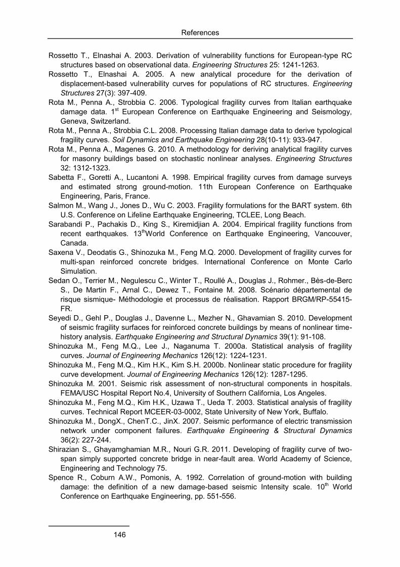
References
146
Rossetto T., Elnashai A. 2003. Derivation of vulnerability functions for European-type RC structures based on observational data. Engineering Structures 25: 1241-1263.
Rossetto T., Elnashai A. 2005. A new analytical procedure for the derivation of displacement-based vulnerability curves for populations of RC structures. Engineering Structures 27(3): 397-409.
Rota M., Penna A., Strobbia C. 2006. Typological fragility curves from Italian earthquake damage data. 1st European Conference on Earthquake Engineering and Seismology, Geneva, Switzerland.
Rota M., Penna A., Strobbia C.L. 2008. Processing Italian damage data to derive typological fragility curves. Soil Dynamics and Earthquake Engineering 28(10-11): 933-947.
Rota M., Penna A., Magenes G. 2010. A methodology for deriving analytical fragility curves for masonry buildings based on stochastic nonlinear analyses. Engineering Structures 32: 1312-1323.
Sabetta F., Goretti A., Lucantoni A. 1998. Empirical fragility curves from damage surveys and estimated strong ground-motion. 11th European Conference on Earthquake Engineering, Paris, France.
Salmon M., Wang J., Jones D., Wu C. 2003. Fragility formulations for the BART system. 6th U.S. Conference on Lifeline Earthquake Engineering, TCLEE, Long Beach.
Sarabandi P., Pachakis D., King S., Kiremidjian A. 2004. Empirical fragility functions from recent earthquakes. 13thWorld Conference on Earthquake Engineering, Vancouver, Canada.
Saxena V., Deodatis G., Shinozuka M., Feng M.Q. 2000. Development of fragility curves for multi-span reinforced concrete bridges. International Conference on Monte Carlo Simulation.
Sedan O., Terrier M., Negulescu C., Winter T., Roullé A., Douglas J., Rohmer., Bès-de-Berc S., De Martin F., Arnal C., Dewez T., Fontaine M. 2008. Scénario départemental de risque sismique- Méthodologie et processus de réalisation. Rapport BRGM/RP-55415-FR.
Seyedi D., Gehl P., Douglas J., Davenne L., Mezher N., Ghavamian S. 2010. Development of seismic fragility surfaces for reinforced concrete buildings by means of nonlinear time-history analysis. Earthquake Engineering and Structural Dynamics 39(1): 91-108.
Shinozuka M., Feng M.Q., Lee J., Naganuma T. 2000a. Statistical analysis of fragility curves. Journal of Engineering Mechanics 126(12): 1224-1231.
Shinozuka M., Feng M.Q., Kim H.K., Kim S.H. 2000b. Nonlinear static procedure for fragility curve development. Journal of Engineering Mechanics 126(12): 1287-1295.
Shinozuka M. 2001. Seismic risk assessment of non-structural components in hospitals. FEMA/USC Hospital Report No.4, University of Southern California, Los Angeles.
Shinozuka M., Feng M.Q., Kim H.K., Uzawa T., Ueda T. 2003. Statistical analysis of fragility curves. Technical Report MCEER-03-0002, State University of New York, Buffalo.
Shinozuka M., DongX., ChenT.C., JinX. 2007. Seismic performance of electric transmission network under component failures. Earthquake Engineering & Structural Dynamics 36(2): 227-244.
Shirazian S., Ghayamghamian M.R., Nouri G.R. 2011. Developing of fragility curve of two-span simply supported concrete bridge in near-fault area. World Academy of Science, Engineering and Technology 75.
Spence R., Coburn A.W., Pomonis, A. 1992. Correlation of ground-motion with building damage: the definition of a new damage-based seismic Intensity scale. 10th World Conference on Earthquake Engineering, pp. 551-556.
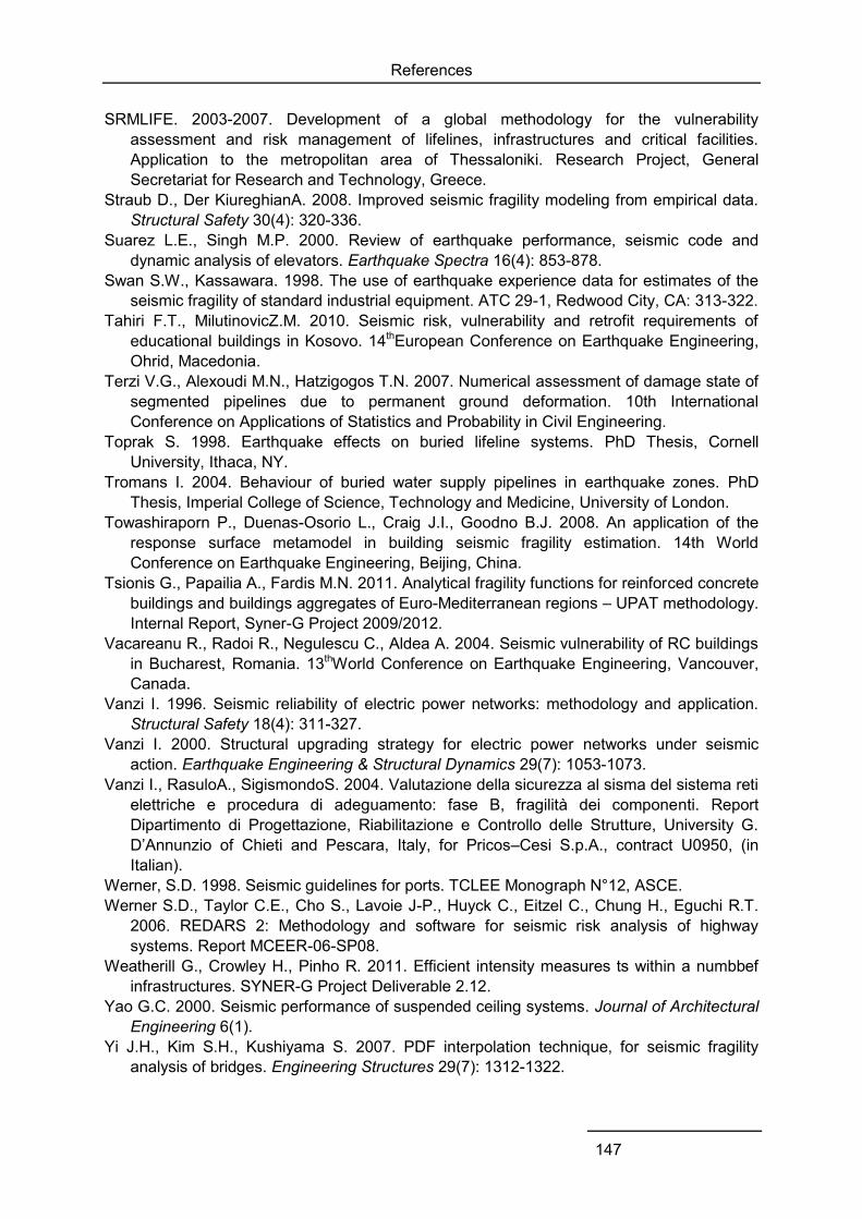
References
147
SRMLIFE. 2003-2007. Development of a global methodology for the vulnerability assessment and risk management of lifelines, infrastructures and critical facilities. Application to the metropolitan area of Thessaloniki. Research Project, General Secretariat for Research and Technology, Greece.
Straub D., Der KiureghianA. 2008. Improved seismic fragility modeling from empirical data. Structural Safety 30(4): 320-336.
Suarez L.E., Singh M.P. 2000. Review of earthquake performance, seismic code and dynamic analysis of elevators. Earthquake Spectra 16(4): 853-878.
Swan S.W., Kassawara. 1998. The use of earthquake experience data for estimates of the seismic fragility of standard industrial equipment. ATC 29-1, Redwood City, CA: 313-322.
Tahiri F.T., MilutinovicZ.M. 2010. Seismic risk, vulnerability and retrofit requirements of educational buildings in Kosovo. 14thEuropean Conference on Earthquake Engineering, Ohrid, Macedonia.
Terzi V.G., Alexoudi M.N., Hatzigogos T.N. 2007. Numerical assessment of damage state of segmented pipelines due to permanent ground deformation. 10th International Conference on Applications of Statistics and Probability in Civil Engineering.
Toprak S. 1998. Earthquake effects on buried lifeline systems. PhD Thesis, Cornell University, Ithaca, NY.
Tromans I. 2004. Behaviour of buried water supply pipelines in earthquake zones. PhD Thesis, Imperial College of Science, Technology and Medicine, University of London.
Towashiraporn P., Duenas-Osorio L., Craig J.I., Goodno B.J. 2008. An application of the response surface metamodel in building seismic fragility estimation. 14th World Conference on Earthquake Engineering, Beijing, China.
Tsionis G., Papailia A., Fardis M.N. 2011. Analytical fragility functions for reinforced concrete buildings and buildings aggregates of Euro-Mediterranean regions – UPAT methodology. Internal Report, Syner-G Project 2009/2012.
Vacareanu R., Radoi R., Negulescu C., Aldea A. 2004. Seismic vulnerability of RC buildings in Bucharest, Romania. 13thWorld Conference on Earthquake Engineering, Vancouver, Canada.
Vanzi I. 1996. Seismic reliability of electric power networks: methodology and application. Structural Safety 18(4): 311-327.
Vanzi I. 2000. Structural upgrading strategy for electric power networks under seismic action. Earthquake Engineering & Structural Dynamics 29(7): 1053-1073.
Vanzi I., RasuloA., SigismondoS. 2004. Valutazione della sicurezza al sisma del sistema reti elettriche e procedura di adeguamento: fase B, fragilità dei componenti. Report Dipartimento di Progettazione, Riabilitazione e Controllo delle Strutture, University G. D’Annunzio of Chieti and Pescara, Italy, for Pricos–Cesi S.p.A., contract U0950, (in Italian).
Werner, S.D. 1998. Seismic guidelines for ports. TCLEE Monograph N°12, ASCE. Werner S.D., Taylor C.E., Cho S., Lavoie J-P., Huyck C., Eitzel C., Chung H., Eguchi R.T.
2006. REDARS 2: Methodology and software for seismic risk analysis of highway systems. Report MCEER-06-SP08.
Weatherill G., Crowley H., Pinho R. 2011. Efficient intensity measures ts within a numbbef infrastructures. SYNER-G Project Deliverable 2.12.
Yao G.C. 2000. Seismic performance of suspended ceiling systems. Journal of Architectural Engineering 6(1).
Yi J.H., Kim S.H., Kushiyama S. 2007. PDF interpolation technique, for seismic fragility analysis of bridges. Engineering Structures 29(7): 1312-1322.

References
148

Proposed fragility curves for buildings
149
Appendix A
A Proposed fragility curves for buildings
A.1 RC BUILDINGS
The following figures show the comparison of the yield and collapse limit state, respectively, for four reinforced concrete buildings classes.
(a) (b)
Fig. A.1 Yield limit state (a) and collapse limit state (b) harmonised fragility functions for a reinforced concrete mid-rise building with moment resisting frame
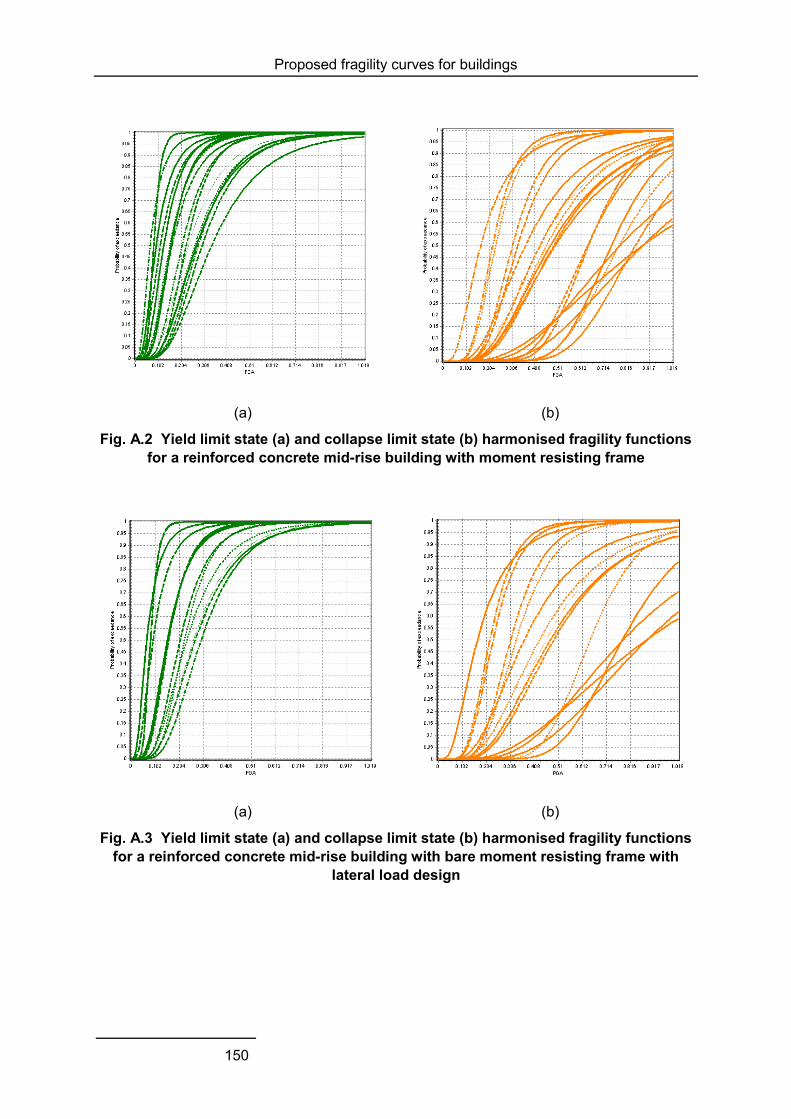
Proposed fragility curves for buildings
150
(a) (b)
Fig. A.2 Yield limit state (a) and collapse limit state (b) harmonised fragility functions for a reinforced concrete mid-rise building with moment resisting frame
(a) (b)
Fig. A.3 Yield limit state (a) and collapse limit state (b) harmonised fragility functions for a reinforced concrete mid-rise building with bare moment resisting frame with
lateral load design
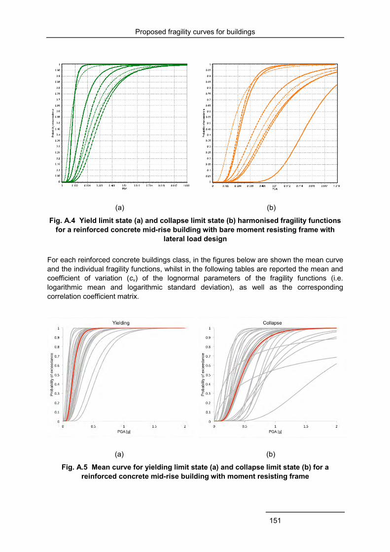
Proposed fragility curves for buildings
151
(a) (b)
Fig. A.4 Yield limit state (a) and collapse limit state (b) harmonised fragility functions for a reinforced concrete mid-rise building with bare moment resisting frame with
lateral load design
For each reinforced concrete buildings class, in the figures below are shown the mean curve and the individual fragility functions, whilst in the following tables are reported the mean and coefficient of variation (cv) of the lognormal parameters of the fragility functions (i.e. logarithmic mean and logarithmic standard deviation), as well as the corresponding correlation coefficient matrix.
(a) (b)
Fig. A.5 Mean curve for yielding limit state (a) and collapse limit state (b) for a reinforced concrete mid-rise building with moment resisting frame
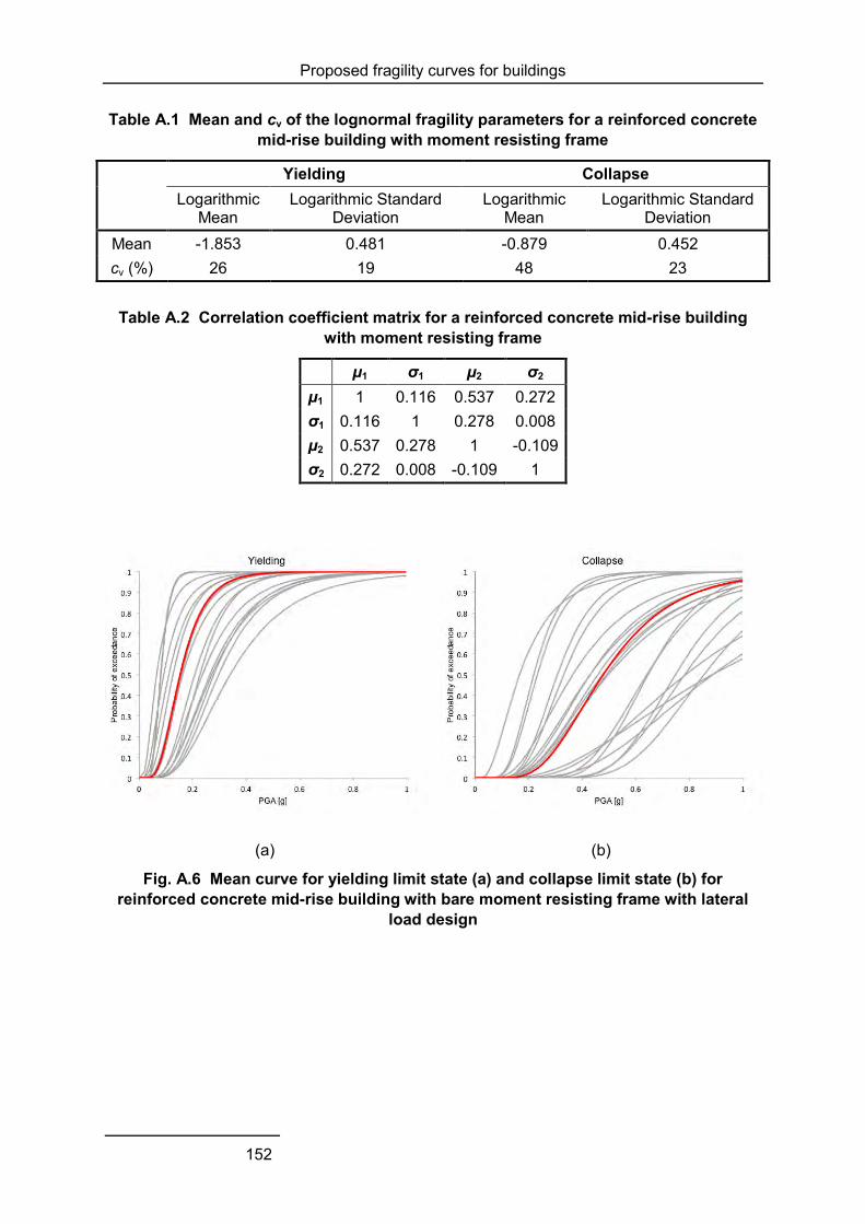
Proposed fragility curves for buildings
152
Table A.1 Mean and cv of the lognormal fragility parameters for a reinforced concrete mid-rise building with moment resisting frame
Yielding Collapse Logarithmic
Mean Logarithmic Standard
Deviation Logarithmic
Mean Logarithmic Standard
Deviation Mean -1.853 0.481 -0.879 0.452 cv (%) 26 19 48 23
Table A.2 Correlation coefficient matrix for a reinforced concrete mid-rise building with moment resisting frame
μ1 σ1 μ2 σ2 μ1 1 0.116 0.537 0.272 σ1 0.116 1 0.278 0.008 μ2 0.537 0.278 1 -0.109 σ2 0.272 0.008 -0.109 1
(a) (b)
Fig. A.6 Mean curve for yielding limit state (a) and collapse limit state (b) for reinforced concrete mid-rise building with bare moment resisting frame with lateral
load design
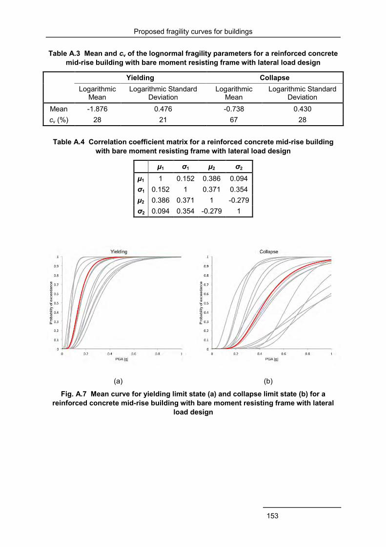
Proposed fragility curves for buildings
153
Table A.3 Mean and cv of the lognormal fragility parameters for a reinforced concrete mid-rise building with bare moment resisting frame with lateral load design
Yielding Collapse Logarithmic
Mean Logarithmic Standard
Deviation Logarithmic
Mean Logarithmic Standard
Deviation Mean -1.876 0.476 -0.738 0.430 cv (%) 28 21 67 28
Table A.4 Correlation coefficient matrix for a reinforced concrete mid-rise building with bare moment resisting frame with lateral load design
μ1 σ1 μ2 σ2 μ1 1 0.152 0.386 0.094 σ1 0.152 1 0.371 0.354 μ2 0.386 0.371 1 -0.279 σ2 0.094 0.354 -0.279 1
(a) (b)
Fig. A.7 Mean curve for yielding limit state (a) and collapse limit state (b) for a reinforced concrete mid-rise building with bare moment resisting frame with lateral
load design
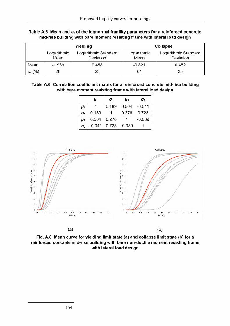
Proposed fragility curves for buildings
154
Table A.5 Mean and cv of the lognormal fragility parameters for a reinforced concrete mid-rise building with bare moment resisting frame with lateral load design
Yielding Collapse Logarithmic
Mean Logarithmic Standard
Deviation Logarithmic
Mean Logarithmic Standard
Deviation Mean -1.939 0.458 -0.821 0.452 cv (%) 28 23 64 25
Table A.6 Correlation coefficient matrix for a reinforced concrete mid-rise building with bare moment resisting frame with lateral load design
μ1 σ1 μ2 σ2 μ1 1 0.189 0.504 -0.041 σ1 0.189 1 0.276 0.723 μ2 0.504 0.276 1 -0.089 σ2 -0.041 0.723 -0.089 1
(a) (b)
Fig. A.8 Mean curve for yielding limit state (a) and collapse limit state (b) for a reinforced concrete mid-rise building with bare non-ductile moment resisting frame
with lateral load design
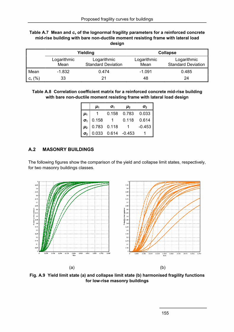
Proposed fragility curves for buildings
155
Table A.7 Mean and cv of the lognormal fragility parameters for a reinforced concrete mid-rise building with bare non-ductile moment resisting frame with lateral load
design
Yielding Collapse Logarithmic
Mean Logarithmic
Standard Deviation Logarithmic
Mean Logarithmic
Standard Deviation Mean -1.832 0.474 -1.091 0.485 cv (%) 33 21 48 24
Table A.8 Correlation coefficient matrix for a reinforced concrete mid-rise building with bare non-ductile moment resisting frame with lateral load design
μ1 σ1 μ2 σ2 μ1 1 0.158 0.783 0.033 σ1 0.158 1 0.118 0.614 μ2 0.783 0.118 1 -0.453 σ2 0.033 0.614 -0.453 1
A.2 MASONRY BUILDINGS
The following figures show the comparison of the yield and collapse limit states, respectively, for two masonry buildings classes.
(a) (b)
Fig. A.9 Yield limit state (a) and collapse limit state (b) harmonised fragility functions for low-rise masonry buildings
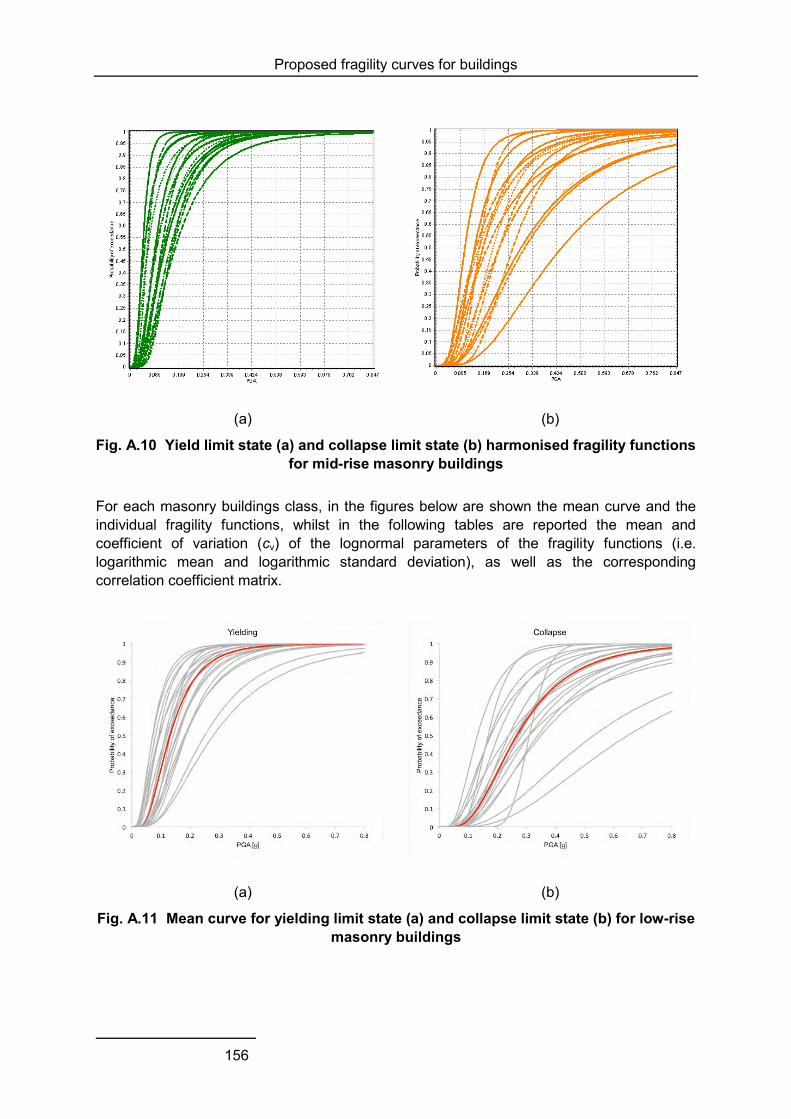
Proposed fragility curves for buildings
156
(a) (b)
Fig. A.10 Yield limit state (a) and collapse limit state (b) harmonised fragility functions for mid-rise masonry buildings
For each masonry buildings class, in the figures below are shown the mean curve and the individual fragility functions, whilst in the following tables are reported the mean and coefficient of variation (cv) of the lognormal parameters of the fragility functions (i.e. logarithmic mean and logarithmic standard deviation), as well as the corresponding correlation coefficient matrix.
(a) (b)
Fig. A.11 Mean curve for yielding limit state (a) and collapse limit state (b) for low-rise masonry buildings

Proposed fragility curves for buildings
157
Table A.9 Mean and cv of the lognormal fragility parameters for low-rise masonry buildings
Yielding Collapse Logarithmic
Mean Logarithmic Standard
Deviation Logarithmic
Mean Logarithmic Standard
Deviation Mean -2.029 0.572 -1.320 0.552 cv (%) 19 16 28 24
Table A.10 Correlation coefficient matrix for low-rise masonry buildings
μ1 σ1 μ2 σ2 μ1 1 -0.220 0.647 -0.051 σ1 -0.220 1 0.119 0.709 μ2 0.647 0.119 1 0.199 σ2 -0.051 0.709 0.199 1
(a) (b)
Fig. A.12 Mean curve for yielding limit state (a) and collapse limit state (b) for mid-rise masonry buildings
Table A.11 Mean and cv of the lognormal fragility parameters for mid-rise masonry buildings
Yielding Collapse Logarithmic
Mean Logarithmic Standard
Deviation Logarithmic
Mean Logarithmic Standard
Deviation Mean -2.417 0.587 -1.5984 0.5732 cv (%) 17 16 24 21

Proposed fragility curves for buildings
158
Table A.12 Correlation coefficient matrix for mid-rise masonry buildings
μ1 σ1 μ2 σ2 μ1 1 -0.045 0.725 -0.244 σ1 -0.045 1 0.377 0.830 μ2 0.725 0.377 1 0.141 σ2 -0.244 0.830 0.141 1
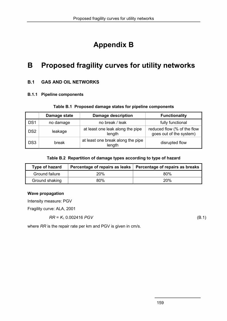
Proposed fragility curves for utility networks
159
Appendix B
B Proposed fragility curves for utility networks
B.1 GAS AND OIL NETWORKS
B.1.1 Pipeline components
Table B.1 Proposed damage states for pipeline components
Damage state Damage description Functionality DS1 no damage no break / leak fully functional
DS2 leakage at least one leak along the pipe length
reduced flow (% of the flow goes out of the system)
DS3 break at least one break along the pipe length disrupted flow
Table B.2 Repartition of damage types according to type of hazard
Type of hazard Percentage of repairs as leaks Percentage of repairs as breaks Ground failure 20% 80%
Ground shaking 80% 20%
Wave propagation
Intensity measure: PGV
Fragility curve: ALA, 2001
RR = K1 0.002416 PGV (B.1)
where RR is the repair rate per km and PGV is given in cm/s.

Proposed fragility curves for utility networks
160
Fig. B.1 Proposed fragility curves for most common gas and oil pipeline typologies
(ALA, 2001), for wave propagation
Table B.3 Values of correction factor K1 (ALA, 2001)
pipe material joint type soil diameter K1 CI cast-iron
cement unknown small (<30cm) 1.0 cement corrosive small 1.4 cement non corrosive small 0.7
rubber gasket unknown small 0.8 arc welded unknown small 0.6
arc welded corrosive small 0.9 arc welded non corrosive small 0.3 arc welded all large (>30cm) 0.15
rubber gasket unknown small 0.7 screwed all small 1.3 riveted all small 1.3
AC asbestos-cement
rubber gasket all small 0.5 cement all small 1.0
C concrete
welded all large 0.7 cement all large 1.0
rubber gasket all large 0.8 PVC rubber gasket all small 0.5 DI ductile iron
rubber gasket all small 0.5

Proposed fragility curves for utility networks
161
Permanent ground deformation
Intensity measure type: PGD
Fragility curve: ALA, 2001
RR = K2 2.5831 PGD0.319 (B.2)
where RR is the repair rate per km and PGD is given in cm.
Table B.4 Values of correction factor K2 (ALA, 2001)
pipe material joint type K2 Unknown Unknown 1.0
CI cement 1.0
rubber gasket 0.8 mechanical restrained 0.7
WS arc-welded, lap welds 0.15
rubber gasket 0.7
AC rubber gasket 0.8
cement 1.0
Concrete welded 0.6 cement 1.0
rubber gasket 0.7 PVC rubber gasket 0.8 DI rubber gasket 0.5
Fig. B.2 Proposed fragility curves for most common gas and oil pipeline typologies
(ALA, 2001), for permanent ground deformation
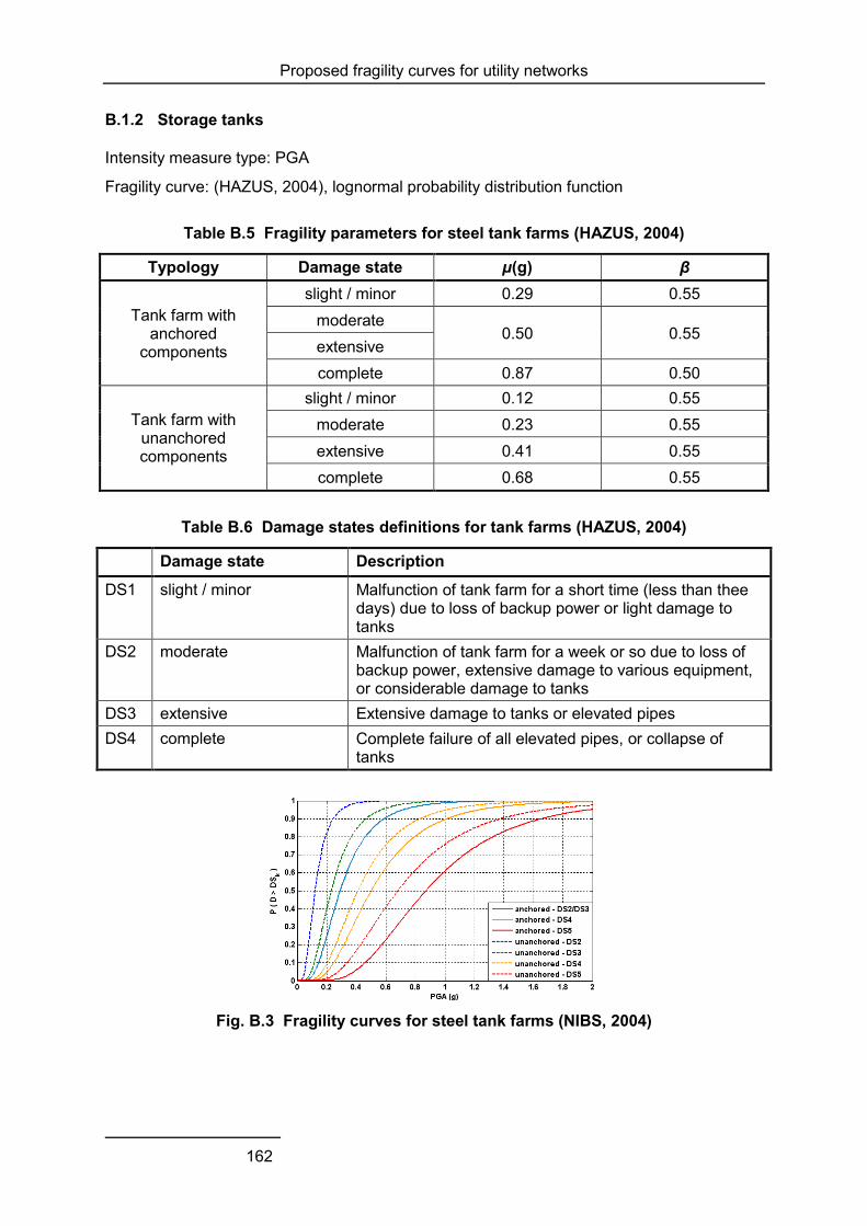
Proposed fragility curves for utility networks
162
B.1.2 Storage tanks
Intensity measure type: PGA
Fragility curve: (HAZUS, 2004), lognormal probability distribution function
Table B.5 Fragility parameters for steel tank farms (HAZUS, 2004)
Typology Damage state µ(g) β
Tank farm with anchored
components
slight / minor 0.29 0.55 moderate
0.50 0.55 extensive complete 0.87 0.50
Tank farm with unanchored components
slight / minor 0.12 0.55 moderate 0.23 0.55 extensive 0.41 0.55 complete 0.68 0.55
Table B.6 Damage states definitions for tank farms (HAZUS, 2004)
Damage state Description
DS1 slight / minor Malfunction of tank farm for a short time (less than thee days) due to loss of backup power or light damage to tanks
DS2 moderate Malfunction of tank farm for a week or so due to loss of backup power, extensive damage to various equipment, or considerable damage to tanks
DS3 extensive Extensive damage to tanks or elevated pipes DS4 complete Complete failure of all elevated pipes, or collapse of
tanks
Fig. B.3 Fragility curves for steel tank farms (NIBS, 2004)
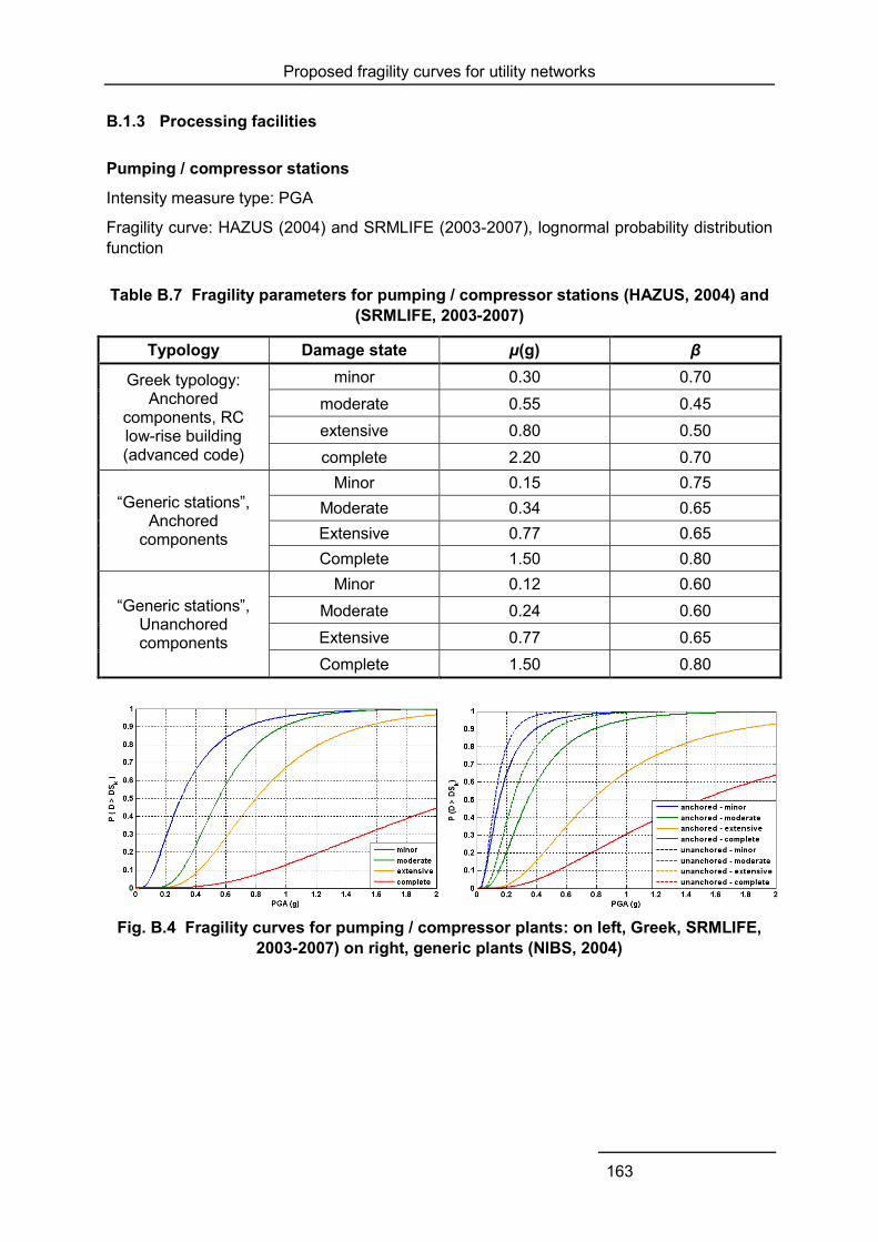
Proposed fragility curves for utility networks
163
B.1.3 Processing facilities
Pumping / compressor stations
Intensity measure type: PGA
Fragility curve: HAZUS (2004) and SRMLIFE (2003-2007), lognormal probability distribution function
Table B.7 Fragility parameters for pumping / compressor stations (HAZUS, 2004) and (SRMLIFE, 2003-2007)
Typology Damage state µ(g) β
Greek typology: Anchored
components, RC low-rise building (advanced code)
minor 0.30 0.70 moderate 0.55 0.45 extensive 0.80 0.50 complete 2.20 0.70
“Generic stations”, Anchored
components
Minor 0.15 0.75 Moderate 0.34 0.65 Extensive 0.77 0.65 Complete 1.50 0.80
“Generic stations”, Unanchored components
Minor 0.12 0.60 Moderate 0.24 0.60 Extensive 0.77 0.65 Complete 1.50 0.80
Fig. B.4 Fragility curves for pumping / compressor plants: on left, Greek, SRMLIFE, 2003-2007) on right, generic plants (NIBS, 2004)
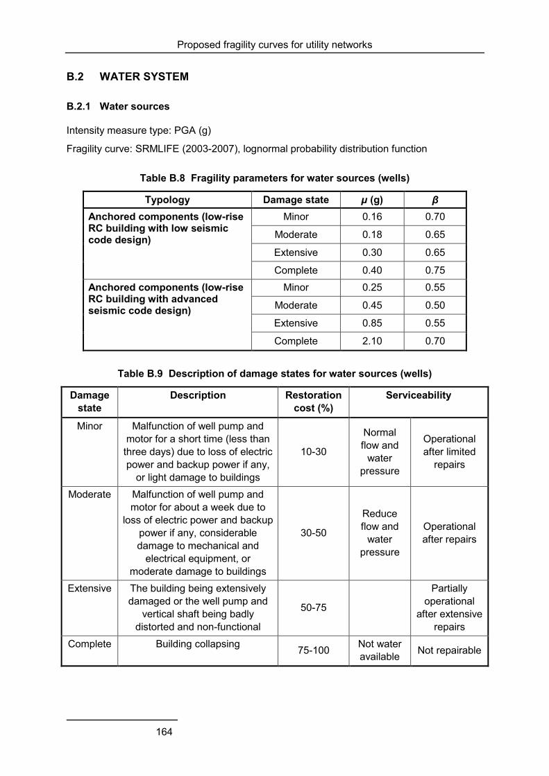
Proposed fragility curves for utility networks
164
B.2 WATER SYSTEM
B.2.1 Water sources
Intensity measure type: PGA (g)
Fragility curve: SRMLIFE (2003-2007), lognormal probability distribution function
Table B.8 Fragility parameters for water sources (wells)
Typology Damage state µ (g) β Anchored components (low-rise RC building with low seismic code design)
Minor 0.16 0.70
Moderate 0.18 0.65
Extensive 0.30 0.65
Complete 0.40 0.75
Anchored components (low-rise RC building with advanced seismic code design)
Minor 0.25 0.55
Moderate 0.45 0.50
Extensive 0.85 0.55
Complete 2.10 0.70
Table B.9 Description of damage states for water sources (wells)
Damage state
Description Restoration cost (%)
Serviceability
Minor Malfunction of well pump and motor for a short time (less than
three days) due to loss of electric power and backup power if any,
or light damage to buildings
10-30
Normal flow and
water pressure
Operational after limited
repairs
Moderate Malfunction of well pump and motor for about a week due to
loss of electric power and backup power if any, considerable damage to mechanical and
electrical equipment, or moderate damage to buildings
30-50
Reduce flow and
water pressure
Operational after repairs
Extensive The building being extensively damaged or the well pump and
vertical shaft being badly distorted and non-functional
50-75
Partially operational
after extensive repairs
Complete Building collapsing 75-100 Not water available Not repairable
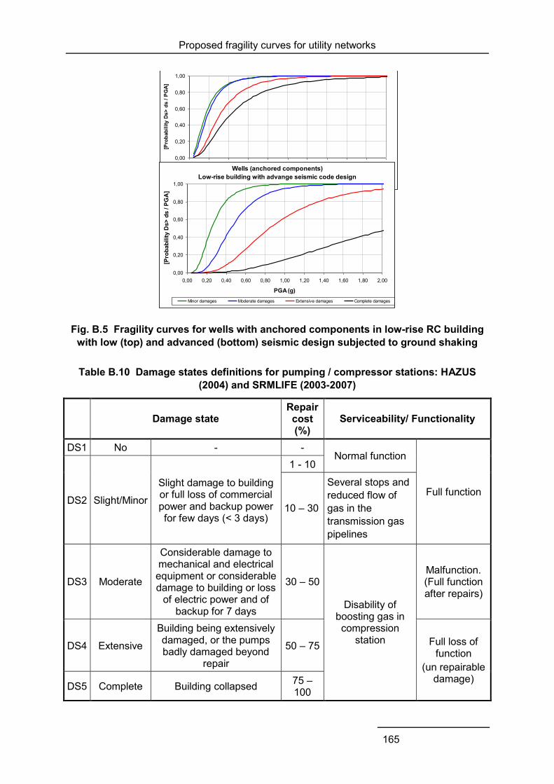
Proposed fragility curves for utility networks
165
Fig. B.5 Fragility curves for wells with anchored components in low-rise RC building
with low (top) and advanced (bottom) seismic design subjected to ground shaking
Table B.10 Damage states definitions for pumping / compressor stations: HAZUS (2004) and SRMLIFE (2003-2007)
Damage state
Repair cost (%)
Serviceability/ Functionality
DS1 No - - Normal function
Full function DS2 Slight/Minor
Slight damage to building or full loss of commercial power and backup power for few days (< 3 days)
1 - 10
10 – 30
Several stops and reduced flow of gas in the transmission gas pipelines
DS3 Moderate
Considerable damage to mechanical and electrical equipment or considerable damage to building or loss
of electric power and of backup for 7 days
30 – 50
Disability of boosting gas in compression
station
Malfunction. (Full function after repairs)
DS4 Extensive
Building being extensively damaged, or the pumps badly damaged beyond
repair
50 – 75 Full loss of function
(un repairable damage)
DS5 Complete Building collapsed 75 – 100
Wells (anchored components) Low-rise building with low seismic code design
0,00
0,20
0,40
0,60
0,80
1,00
0,00 0,20 0,40 0,60 0,80 1,00 1,20 1,40 1,60 1,80 2,00
PGA (g)
[Pro
babi
lity
Ds>
ds /
PGA]
Minor damages Moderate damages Extensive damages Complete damages
Wells (anchored components) Low-rise building with advange seismic code design
0,00
0,20
0,40
0,60
0,80
1,00
0,00 0,20 0,40 0,60 0,80 1,00 1,20 1,40 1,60 1,80 2,00
PGA (g)
[Pro
babi
lity
Ds>
ds
/ PG
A]
Minor damages Moderate damages Extensive damages Complete damages

Proposed fragility curves for utility networks
166
B.2.2 Water treatment plants
Intensity measure type: PGA (g)
Fragility curve: SRMLIFE (2003-2007), lognormal probability distribution function
Table B.11 Fragility parameters for water treatment plants
Typology Damage state µ (g) β
Water treatment plants with anchored components
Minor 0.15 0.30
Moderate 0.30 0.25
Extensive 0.55 0.60
Complete 0.90 0.55
Table B.12 Description of damage states for water treatment plants
Damage state
Description Restoration cost (%)
Serviceability
Minor Malfunction of plant for a short time (<3 days) due to loss of electric power, considerable
damage to various equipment, light damage to sedimentation
basins, light damage to chlorination tanks, or light damage to chemical tanks. Loss of water
quality may occur.
10-30 Normal flow and water pressure
Operational after limited
repairs
Moderate Malfunction of plant for about a week due to loss of electric power
and backup power if any, extensive damage to various
equipment, considerable damage to sedimentation basins, considerable damage to
chlorination tanks with no loss of contents, or considerable damage to chemical tanks. Loss of water
quality is imminent
30-50
Reduce flow and water pressure
Operational after repairs
Extensive The pipes connecting the different basins and chemical units being
extensively damaged. This type of damage will likely result in the
shutdown of the plant.
50-75
Partially operational
after extensive
repairs
Complete The complete failure of all piping or extensive damage to the filter
gallery 75-100 Not water
available Not
repairable

Proposed fragility curves for utility networks
167
Fig. B.6 Fragility curves for water treatment plant (anchored components) subjected
to ground shaking
B.2.3 Pumping stations
Intensity measure type: PGA (g)
Fragility curve: SRMLIFE (2003-2007), lognormal probability distribution function
Fig. B.7 Fragility curves for pumping stations with anchored components in low-rise RC building with low (up) and advanced (down) seismic design subjected to ground
shaking
Water Treatment Plant (anchored components, without back-up power)
0,000
0,200
0,400
0,600
0,800
1,000
0,00 0,20 0,40 0,60 0,80 1,00 1,20 1,40 1,60 1,80 2,00
PGA (g)
[Pro
babi
lity
Ds>
ds /
PGA]
Minor damages Moderate damages Extensive damages Complete damages
Pumping station(anchored components, low-rise building with low seismic code
design, without back-up power)
0,00
0,25
0,50
0,75
1,00
0,00 0,20 0,40 0,60 0,80 1,00 1,20 1,40 1,60 1,80 2,00
PGA (g)
[Pro
babi
lity
Ds>
ds
/ PG
A]
Minor damages Moderate damages Extensive damages Complete damagesPumping station
(anchored components, low-rise building with advance seismic code design, without back-up power)
0,00
0,25
0,50
0,75
1,00
0,00 0,20 0,40 0,60 0,80 1,00 1,20 1,40 1,60 1,80 2,00
PGA (g)
[Pro
babi
lity
Ds>
ds
/ PG
A]
Minor damages Moderate damages Extensive damages Complete damages
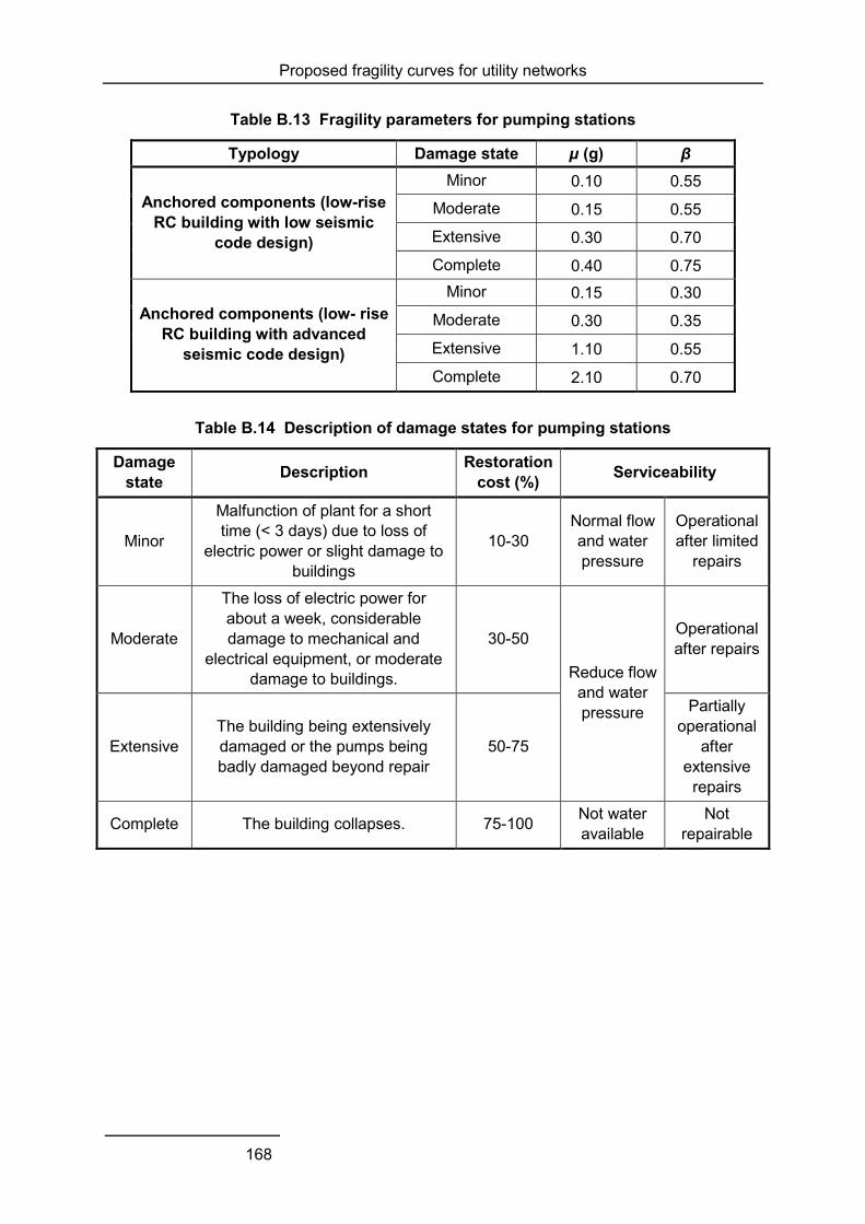
Proposed fragility curves for utility networks
168
Table B.13 Fragility parameters for pumping stations
Typology Damage state µ (g) β
Anchored components (low-rise RC building with low seismic
code design)
Minor 0.10 0.55
Moderate 0.15 0.55
Extensive 0.30 0.70
Complete 0.40 0.75
Anchored components (low- rise RC building with advanced
seismic code design)
Minor 0.15 0.30
Moderate 0.30 0.35
Extensive 1.10 0.55
Complete 2.10 0.70
Table B.14 Description of damage states for pumping stations
Damage state Description Restoration
cost (%) Serviceability
Minor
Malfunction of plant for a short time (< 3 days) due to loss of
electric power or slight damage to buildings
10-30 Normal flow and water pressure
Operational after limited
repairs
Moderate
The loss of electric power for about a week, considerable damage to mechanical and
electrical equipment, or moderate damage to buildings.
30-50
Reduce flow and water pressure
Operational after repairs
Extensive The building being extensively damaged or the pumps being badly damaged beyond repair
50-75
Partially operational
after extensive
repairs
Complete The building collapses. 75-100 Not water available
Not repairable
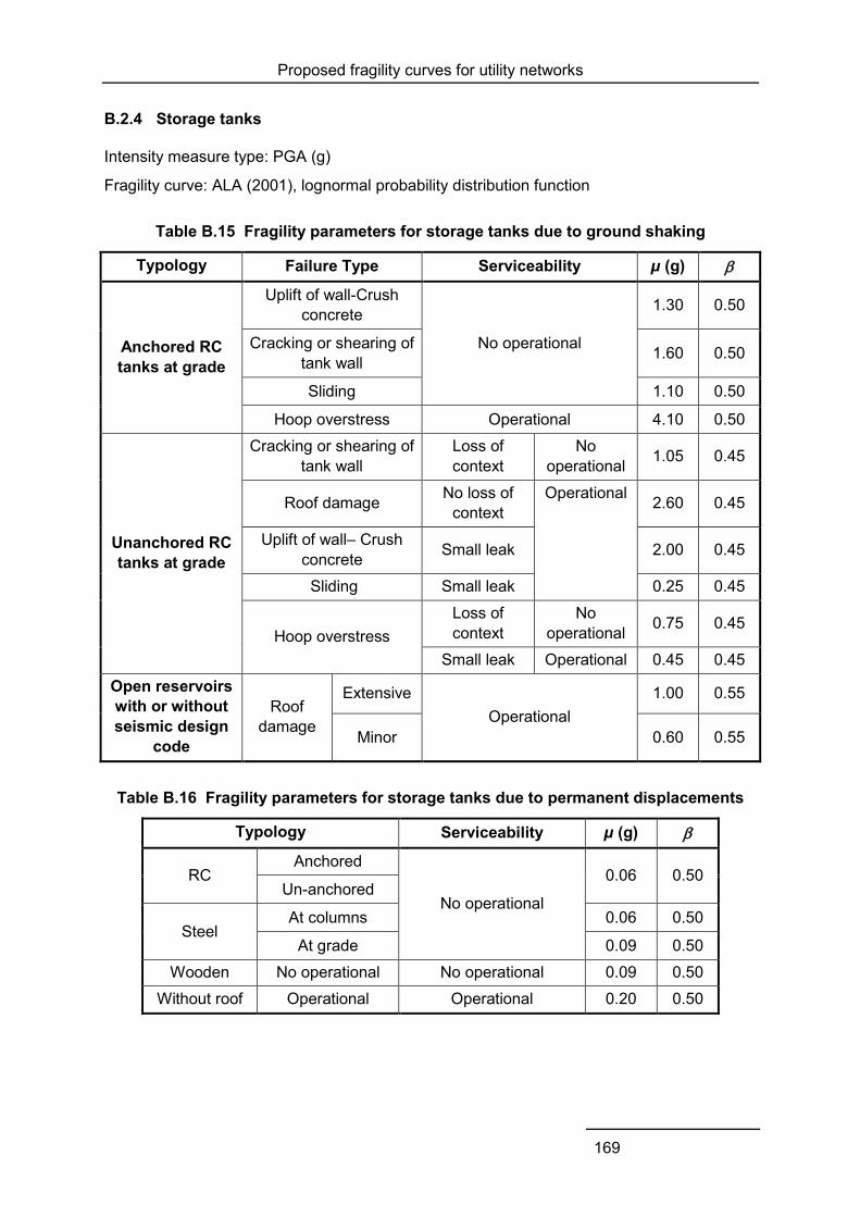
Proposed fragility curves for utility networks
169
B.2.4 Storage tanks
Intensity measure type: PGA (g)
Fragility curve: ALA (2001), lognormal probability distribution function
Table B.15 Fragility parameters for storage tanks due to ground shaking
Typology Failure Type Serviceability µ (g)
Anchored RC tanks at grade
Uplift of wall-Crush concrete
No operational
1.30 0.50
Cracking or shearing of tank wall 1.60 0.50
Sliding 1.10 0.50
Hoop overstress Operational 4.10 0.50
Unanchored RC tanks at grade
Cracking or shearing of tank wall
Loss of context
No operational 1.05 0.45
Roof damage No loss of context
Operational 2.60 0.45
Uplift of wall– Crush concrete Small leak 2.00 0.45
Sliding Small leak 0.25 0.45
Hoop overstress Loss of context
No operational 0.75 0.45
Small leak Operational 0.45 0.45 Open reservoirs with or without seismic design
code
Roof damage
Extensive Operational
1.00 0.55
Minor 0.60 0.55
Table B.16 Fragility parameters for storage tanks due to permanent displacements
Typology Serviceability µ (g)
RC Anchored
No operational
0.06 0.50 Un-anchored
Steel At columns 0.06 0.50
At grade 0.09 0.50 Wooden No operational No operational 0.09 0.50
Without roof Operational Operational 0.20 0.50
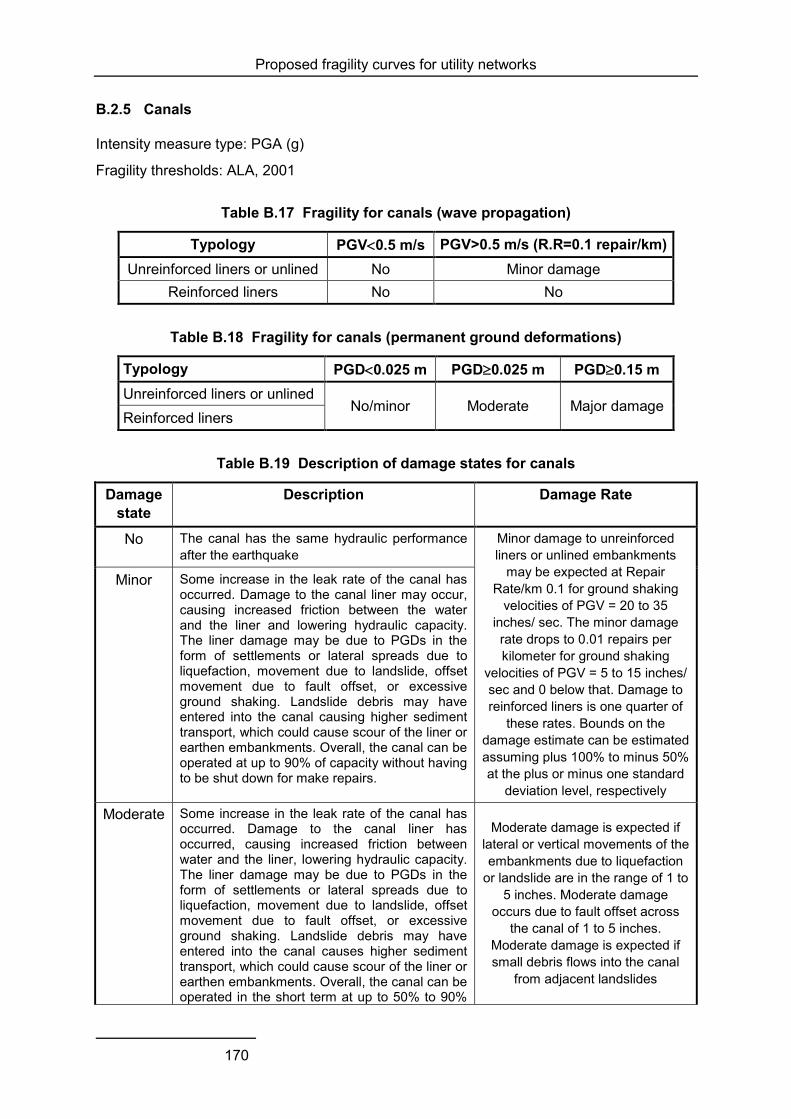
Proposed fragility curves for utility networks
170
B.2.5 Canals
Intensity measure type: PGA (g)
Fragility thresholds: ALA, 2001
Table B.17 Fragility for canals (wave propagation)
Typology PGV0.5 m/s PGV>0.5 m/s (R.R=0.1 repair/km) Unreinforced liners or unlined No Minor damage
Reinforced liners No No
Table B.18 Fragility for canals (permanent ground deformations)
Typology PGD0.025 m PGD0.025 m PGD0.15 m Unreinforced liners or unlined
No/minor Moderate Major damage Reinforced liners
Table B.19 Description of damage states for canals
Damage state
Description Damage Rate
No The canal has the same hydraulic performance after the earthquake
Minor damage to unreinforced liners or unlined embankments
may be expected at Repair Rate/km 0.1 for ground shaking
velocities of PGV = 20 to 35 inches/ sec. The minor damage rate drops to 0.01 repairs per kilometer for ground shaking
velocities of PGV = 5 to 15 inches/ sec and 0 below that. Damage to reinforced liners is one quarter of
these rates. Bounds on the damage estimate can be estimated assuming plus 100% to minus 50% at the plus or minus one standard
deviation level, respectively
Minor Some increase in the leak rate of the canal has occurred. Damage to the canal liner may occur, causing increased friction between the water and the liner and lowering hydraulic capacity. The liner damage may be due to PGDs in the form of settlements or lateral spreads due to liquefaction, movement due to landslide, offset movement due to fault offset, or excessive ground shaking. Landslide debris may have entered into the canal causing higher sediment transport, which could cause scour of the liner or earthen embankments. Overall, the canal can be operated at up to 90% of capacity without having to be shut down for make repairs.
Moderate Some increase in the leak rate of the canal has occurred. Damage to the canal liner has occurred, causing increased friction between water and the liner, lowering hydraulic capacity. The liner damage may be due to PGDs in the form of settlements or lateral spreads due to liquefaction, movement due to landslide, offset movement due to fault offset, or excessive ground shaking. Landslide debris may have entered into the canal causes higher sediment transport, which could cause scour of the liner or earthen embankments. Overall, the canal can be operated in the short term at up to 50% to 90%
Moderate damage is expected if lateral or vertical movements of the embankments due to liquefaction
or landslide are in the range of 1 to 5 inches. Moderate damage
occurs due to fault offset across the canal of 1 to 5 inches.
Moderate damage is expected if small debris flows into the canal
from adjacent landslides

Proposed fragility curves for utility networks
171
of capacity; however, a shutdown of the canal soon after the earthquake will be required to make repairs. Damage to canal overcrossings may have occurred, and temporary shutdown of the canal is needed to make repairs. Damage to bridge abutments could cause constriction of the canal’s cross-section to such an extent that it causes a significant flow restriction.
Major The canal is damaged to such an extent that immediate shutdown is required. The damage may be due to PGDs in the form of settlements or lateral spreads due to liquefaction, movement
due to landslide, offset movement due to fault offset, or excessive ground shaking. Landslide debris may have entered the canal and caused excessive sediment transport, or may block the canal’s cross-section to such a degree that the flow of water is disrupted, overflowing over the
canal’s banks and causing subsequent flooding. Damage to overcrossings may have occurred,
requiring immediate shutdown of the canal. Overcrossing damage could include the collapse of highway bridges and leakage of non-potable material pipelines such as oil, gas, etc. Damage to bridge abutments could cause constriction of
the canal's cross-section to such an extent that a significant flow restriction which warrants
immediate shutdown and repair.
Major damage is expected if PGDs of the embankments are predicted to be six inches or greater. Major damage occurs due to fault offset across the canal of six inches or
more. Major damage is expected if a significant amount of debris is predicted to flow into the canal from adjacent landslides. The
differentiation of moderate or major damage states for debris flows into the canal should factor in hydraulic constraints caused by the size of the debris flow, the potential for
scour due to the type of debris and water quality requirement
B.2.6 Pipes
Intensity measure type: PGD
Fragility curve: Honneger and Eguchi (1992)
RR/km= K*(7.821*PGD0.56) (B.3)
where RR is the repair rate per km and PGD is given in cm.
Table B.20 Values of correction factor K
Typology K
Brittle pipelines 1.0
Ductile pipelines 0.3
Intensity measure type: PGV
Fragility curve: O’Rourke and Ayala (1993)
RR/km= K*(0.0001*PGV2.25) (B.4)
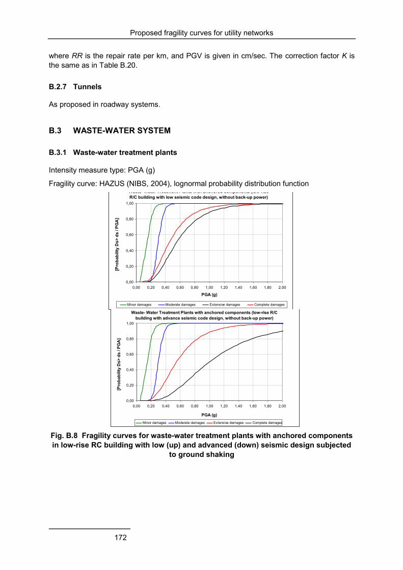
Proposed fragility curves for utility networks
172
where RR is the repair rate per km, and PGV is given in cm/sec. The correction factor K is the same as in Table B.20.
B.2.7 Tunnels
As proposed in roadway systems.
B.3 WASTE-WATER SYSTEM
B.3.1 Waste-water treatment plants
Intensity measure type: PGA (g)
Fragility curve: HAZUS (NIBS, 2004), lognormal probability distribution function
Fig. B.8 Fragility curves for waste-water treatment plants with anchored components in low-rise RC building with low (up) and advanced (down) seismic design subjected
to ground shaking
Waste- Water Treatment Plants with anchored components (low-rise R/C building with low seismic code design, without back-up power)
0,00
0,20
0,40
0,60
0,80
1,00
0,00 0,20 0,40 0,60 0,80 1,00 1,20 1,40 1,60 1,80 2,00
PGA (g)
[Pro
babi
lity
Ds>
ds
/ PG
A]
Minor damages Moderate damages Extensive damages Complete damages
Waste- Water Treatment Plants with anchored components (low-rise R/C building with advance seismic code design, without back-up power)
0,00
0,20
0,40
0,60
0,80
1,00
0,00 0,20 0,40 0,60 0,80 1,00 1,20 1,40 1,60 1,80 2,00
PGA (g)
[Pro
babi
lity
Ds>
ds
/ PG
A]
Minor damages Moderate damages Extensive damages Complete damages
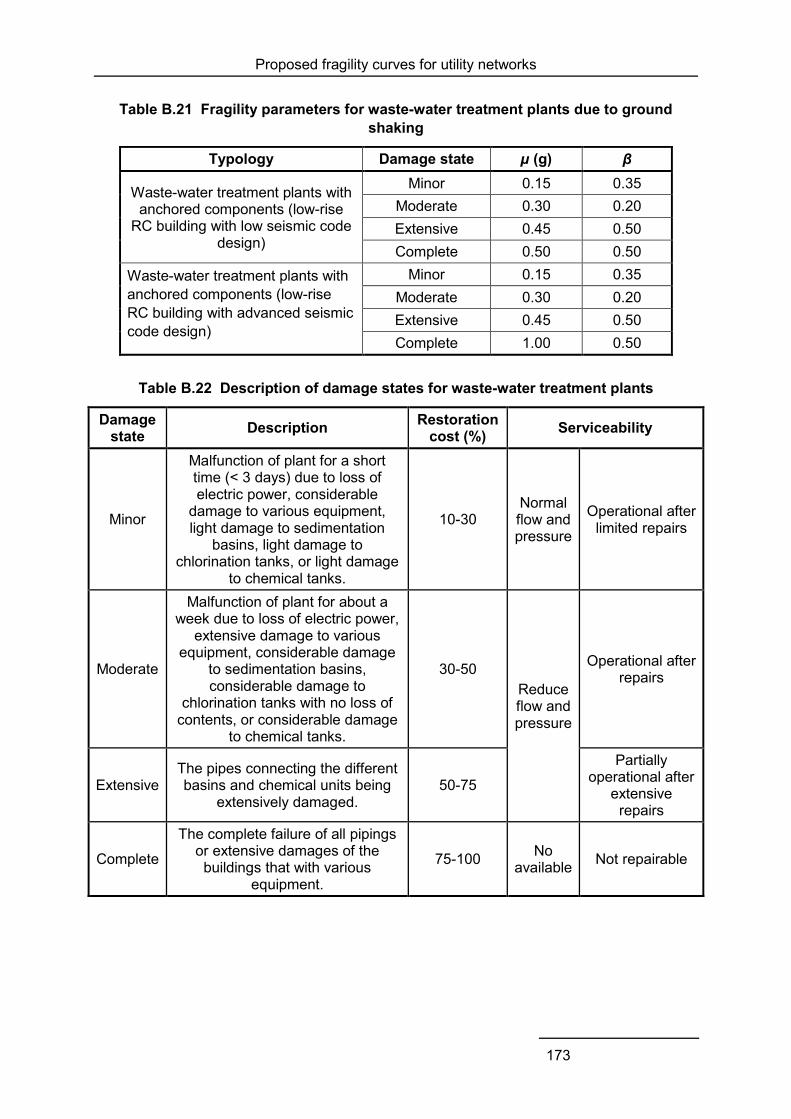
Proposed fragility curves for utility networks
173
Table B.21 Fragility parameters for waste-water treatment plants due to ground shaking
Typology Damage state µ (g) β
Waste-water treatment plants with anchored components (low-rise
RC building with low seismic code design)
Minor 0.15 0.35 Moderate 0.30 0.20 Extensive 0.45 0.50 Complete 0.50 0.50
Waste-water treatment plants with anchored components (low-rise RC building with advanced seismic code design)
Minor 0.15 0.35 Moderate 0.30 0.20 Extensive 0.45 0.50 Complete 1.00 0.50
Table B.22 Description of damage states for waste-water treatment plants
Damage state Description Restoration
cost (%) Serviceability
Minor
Malfunction of plant for a short time (< 3 days) due to loss of electric power, considerable
damage to various equipment, light damage to sedimentation
basins, light damage to chlorination tanks, or light damage
to chemical tanks.
10-30 Normal flow and pressure
Operational after limited repairs
Moderate
Malfunction of plant for about a week due to loss of electric power,
extensive damage to various equipment, considerable damage
to sedimentation basins, considerable damage to
chlorination tanks with no loss of contents, or considerable damage
to chemical tanks.
30-50 Reduce flow and pressure
Operational after repairs
Extensive The pipes connecting the different basins and chemical units being
extensively damaged. 50-75
Partially operational after
extensive repairs
Complete
The complete failure of all pipings or extensive damages of the buildings that with various
equipment.
75-100 No available Not repairable
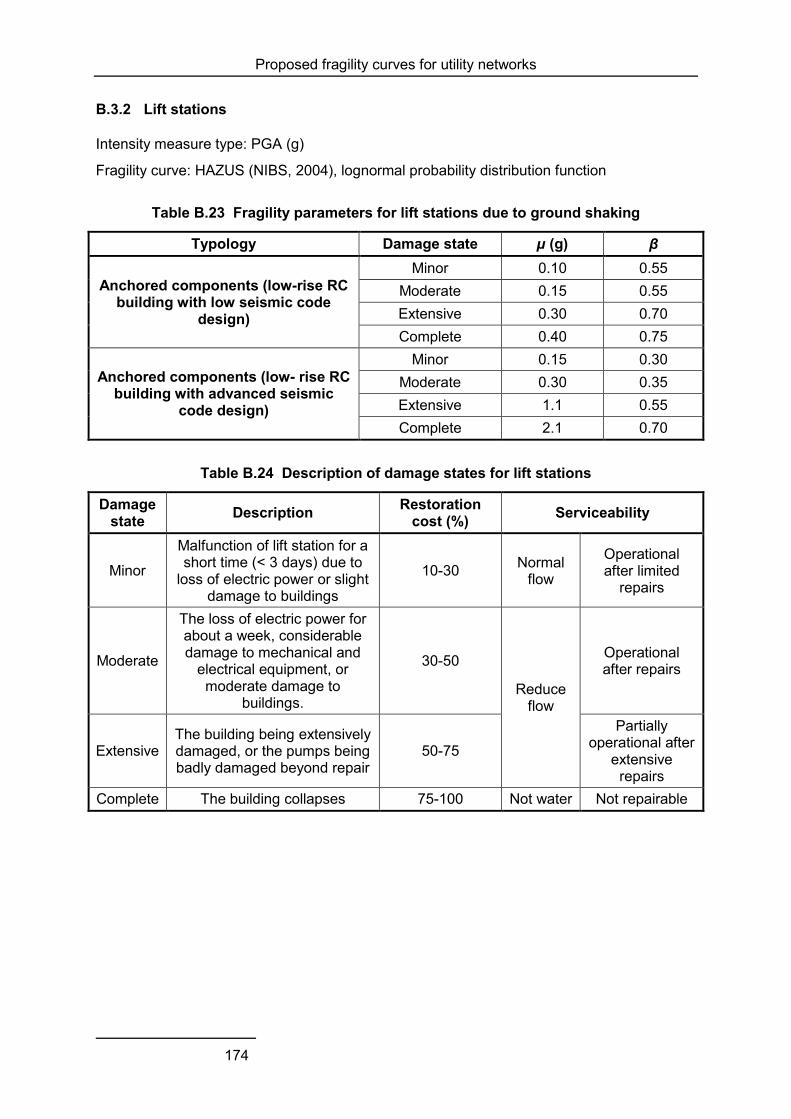
Proposed fragility curves for utility networks
174
B.3.2 Lift stations
Intensity measure type: PGA (g)
Fragility curve: HAZUS (NIBS, 2004), lognormal probability distribution function
Table B.23 Fragility parameters for lift stations due to ground shaking
Typology Damage state µ (g) β
Anchored components (low-rise RC building with low seismic code
design)
Minor 0.10 0.55 Moderate 0.15 0.55 Extensive 0.30 0.70 Complete 0.40 0.75
Anchored components (low- rise RC building with advanced seismic
code design)
Minor 0.15 0.30 Moderate 0.30 0.35 Extensive 1.1 0.55 Complete 2.1 0.70
Table B.24 Description of damage states for lift stations
Damage state Description Restoration
cost (%) Serviceability
Minor
Malfunction of lift station for a short time (< 3 days) due to
loss of electric power or slight damage to buildings
10-30 Normal flow
Operational after limited
repairs
Moderate
The loss of electric power for about a week, considerable damage to mechanical and
electrical equipment, or moderate damage to
buildings.
30-50
Reduce flow
Operational after repairs
Extensive The building being extensively damaged, or the pumps being badly damaged beyond repair
50-75
Partially operational after
extensive repairs
Complete The building collapses 75-100 Not water Not repairable
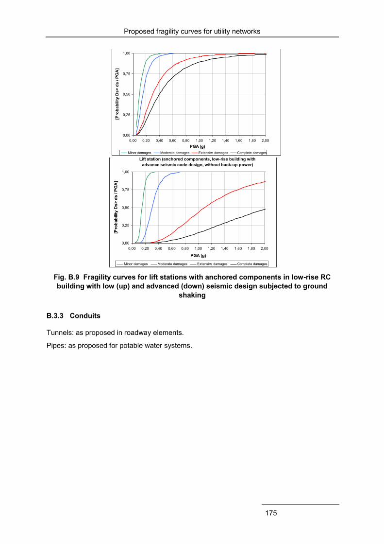
Proposed fragility curves for utility networks
175
Fig. B.9 Fragility curves for lift stations with anchored components in low-rise RC building with low (up) and advanced (down) seismic design subjected to ground
shaking
B.3.3 Conduits
Tunnels: as proposed in roadway elements.
Pipes: as proposed for potable water systems.
Lift station (anchored components, low-rise building with low seismic code design, without back-up power)
0,00
0,25
0,50
0,75
1,00
0,00 0,20 0,40 0,60 0,80 1,00 1,20 1,40 1,60 1,80 2,00PGA (g)
[Pro
babi
lity
Ds>
ds
/ PG
A]
Minor damages Moderate damages Extensive damages Complete damages
Lift station (anchored components, low-rise building with advance seismic code design, without back-up power)
0,00
0,25
0,50
0,75
1,00
0,00 0,20 0,40 0,60 0,80 1,00 1,20 1,40 1,60 1,80 2,00
PGA (g)
[Pro
babi
lity
Ds>
ds
/ PG
A]
Minor damages Moderate damages Extensive damages Complete damages

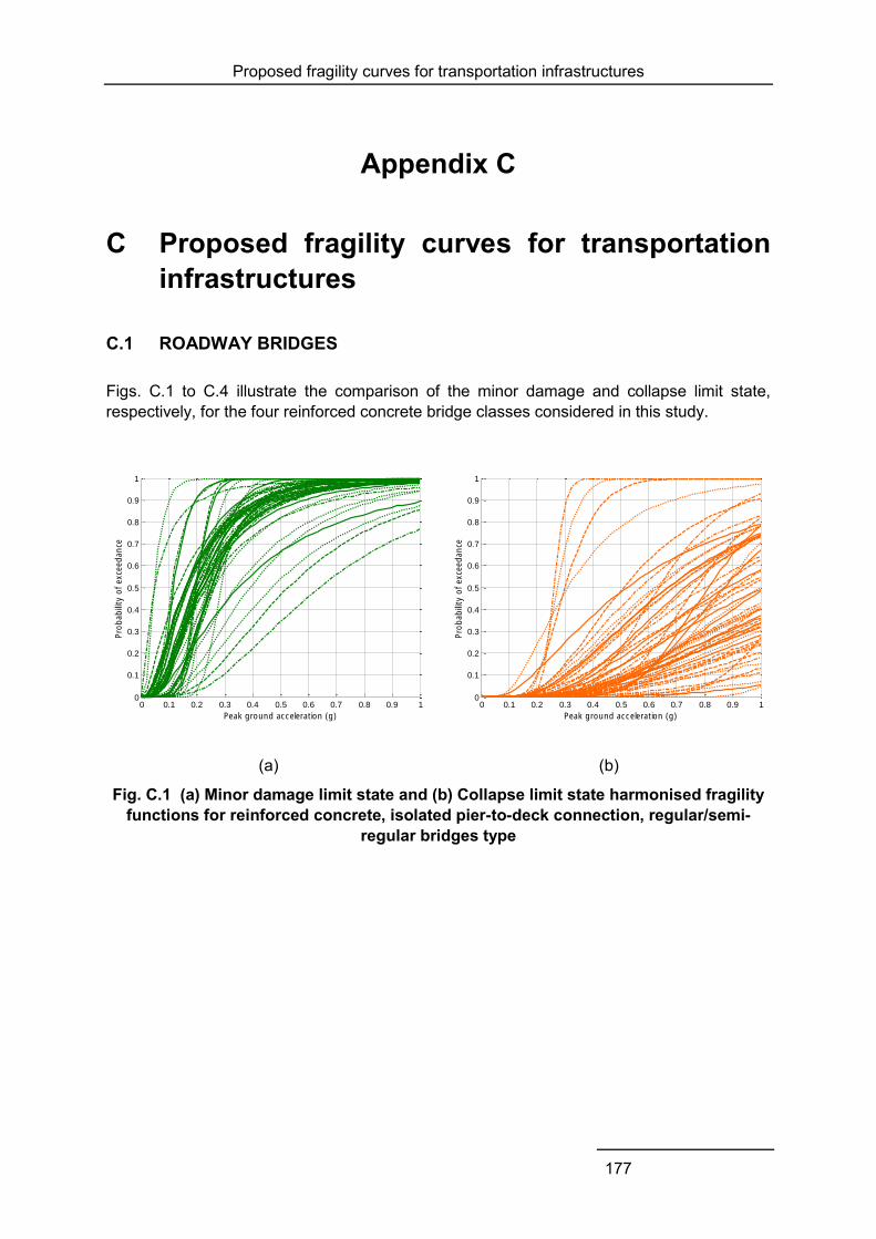
Proposed fragility curves for transportation infrastructures
177
Appendix C
C Proposed fragility curves for transportation infrastructures
C.1 ROADWAY BRIDGES
Figs. C.1 to C.4 illustrate the comparison of the minor damage and collapse limit state, respectively, for the four reinforced concrete bridge classes considered in this study.
(a) (b)
Fig. C.1 (a) Minor damage limit state and (b) Collapse limit state harmonised fragility functions for reinforced concrete, isolated pier-to-deck connection, regular/semi-
regular bridges type
0 0.1 0.2 0.3 0.4 0.5 0.6 0.7 0.8 0.9 10
0.1
0.2
0.3
0.4
0.5
0.6
0.7
0.8
0.9
1
Pro
babili
ty o
f exce
edance
Peak ground acceleration (g)
0 0.1 0.2 0.3 0.4 0.5 0.6 0.7 0.8 0.9 10
0.1
0.2
0.3
0.4
0.5
0.6
0.7
0.8
0.9
1
Pro
babili
ty o
f exce
edance
Peak ground acceleration (g)
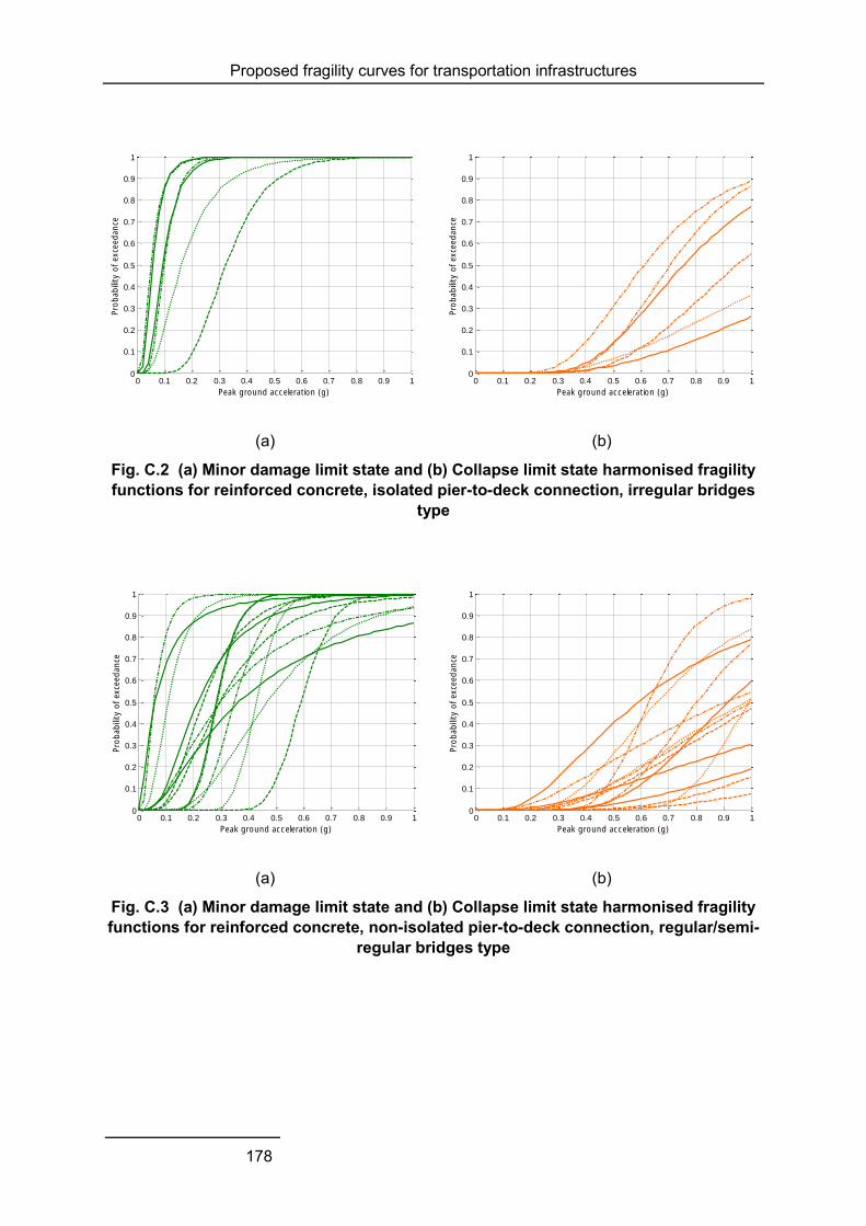
Proposed fragility curves for transportation infrastructures
178
(a) (b)
Fig. C.2 (a) Minor damage limit state and (b) Collapse limit state harmonised fragility functions for reinforced concrete, isolated pier-to-deck connection, irregular bridges
type
(a) (b)
Fig. C.3 (a) Minor damage limit state and (b) Collapse limit state harmonised fragility functions for reinforced concrete, non-isolated pier-to-deck connection, regular/semi-
regular bridges type
0 0.1 0.2 0.3 0.4 0.5 0.6 0.7 0.8 0.9 10
0.1
0.2
0.3
0.4
0.5
0.6
0.7
0.8
0.9
1
Pro
babili
ty o
f exce
edance
Peak ground acceleration (g)
0 0.1 0.2 0.3 0.4 0.5 0.6 0.7 0.8 0.9 10
0.1
0.2
0.3
0.4
0.5
0.6
0.7
0.8
0.9
1
Pro
babili
ty o
f exce
edance
Peak ground acceleration (g)
0 0.1 0.2 0.3 0.4 0.5 0.6 0.7 0.8 0.9 10
0.1
0.2
0.3
0.4
0.5
0.6
0.7
0.8
0.9
1
Pro
babili
ty o
f exce
edance
Peak ground acceleration (g)
0 0.1 0.2 0.3 0.4 0.5 0.6 0.7 0.8 0.9 10
0.1
0.2
0.3
0.4
0.5
0.6
0.7
0.8
0.9
1
Pro
babili
ty o
f exce
edance
Peak ground acceleration (g)
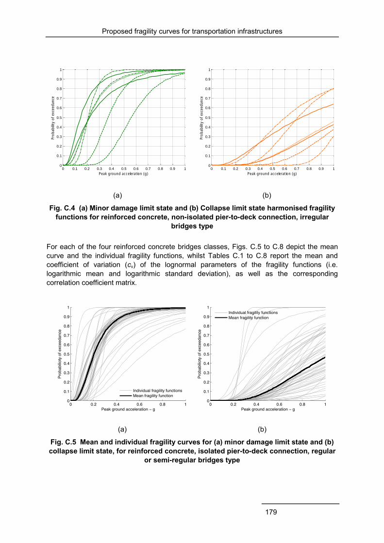
Proposed fragility curves for transportation infrastructures
179
(a) (b)
Fig. C.4 (a) Minor damage limit state and (b) Collapse limit state harmonised fragility functions for reinforced concrete, non-isolated pier-to-deck connection, irregular
bridges type
For each of the four reinforced concrete bridges classes, Figs. C.5 to C.8 depict the mean curve and the individual fragility functions, whilst Tables C.1 to C.8 report the mean and coefficient of variation (cv) of the lognormal parameters of the fragility functions (i.e. logarithmic mean and logarithmic standard deviation), as well as the corresponding correlation coefficient matrix.
(a) (b)
Fig. C.5 Mean and individual fragility curves for (a) minor damage limit state and (b) collapse limit state, for reinforced concrete, isolated pier-to-deck connection, regular
or semi-regular bridges type
0 0.1 0.2 0.3 0.4 0.5 0.6 0.7 0.8 0.9 10
0.1
0.2
0.3
0.4
0.5
0.6
0.7
0.8
0.9
1
Pro
babili
ty o
f exce
edance
Peak ground acceleration (g)
0 0.1 0.2 0.3 0.4 0.5 0.6 0.7 0.8 0.9 10
0.1
0.2
0.3
0.4
0.5
0.6
0.7
0.8
0.9
1
Pro
babili
ty o
f exce
edance
Peak ground acceleration (g)
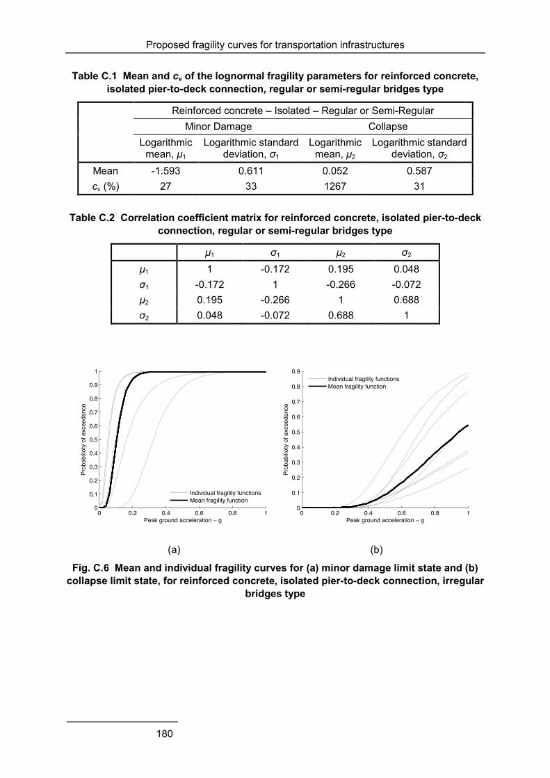
Proposed fragility curves for transportation infrastructures
180
Table C.1 Mean and cv of the lognormal fragility parameters for reinforced concrete, isolated pier-to-deck connection, regular or semi-regular bridges type
Reinforced concrete – Isolated – Regular or Semi-Regular Minor Damage Collapse Logarithmic
mean, μ1 Logarithmic standard
deviation, σ1 Logarithmic
mean, μ2 Logarithmic standard
deviation, σ2 Mean -1.593 0.611 0.052 0.587 cv (%) 27 33 1267 31
Table C.2 Correlation coefficient matrix for reinforced concrete, isolated pier-to-deck connection, regular or semi-regular bridges type
μ1 σ1 μ2 σ2 μ1 1 -0.172 0.195 0.048 σ1 -0.172 1 -0.266 -0.072 μ2 0.195 -0.266 1 0.688 σ2 0.048 -0.072 0.688 1
(a) (b)
Fig. C.6 Mean and individual fragility curves for (a) minor damage limit state and (b) collapse limit state, for reinforced concrete, isolated pier-to-deck connection, irregular
bridges type
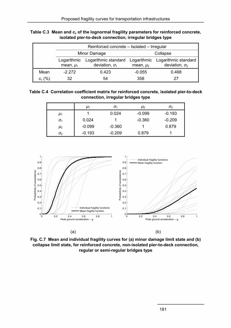
Proposed fragility curves for transportation infrastructures
181
Table C.3 Mean and cv of the lognormal fragility parameters for reinforced concrete, isolated pier-to-deck connection, irregular bridges type
Reinforced concrete – Isolated – Irregular Minor Damage Collapse Logarithmic
mean, μ1 Logarithmic standard
deviation, σ1 Logarithmic
mean, μ2 Logarithmic standard
deviation, σ2 Mean -2.272 0.423 -0.055 0.468 cv (%) 32 54 358 27
Table C.4 Correlation coefficient matrix for reinforced concrete, isolated pier-to-deck connection, irregular bridges type
μ1 σ1 μ2 σ2 μ1 1 0.024 -0.099 -0.193 σ1 0.024 1 -0.360 -0.209 μ2 -0.099 -0.360 1 0.879 σ2 -0.193 -0.209 0.879 1
(a) (b)
Fig. C.7 Mean and individual fragility curves for (a) minor damage limit state and (b) collapse limit state, for reinforced concrete, non-isolated pier-to-deck connection,
regular or semi-regular bridges type
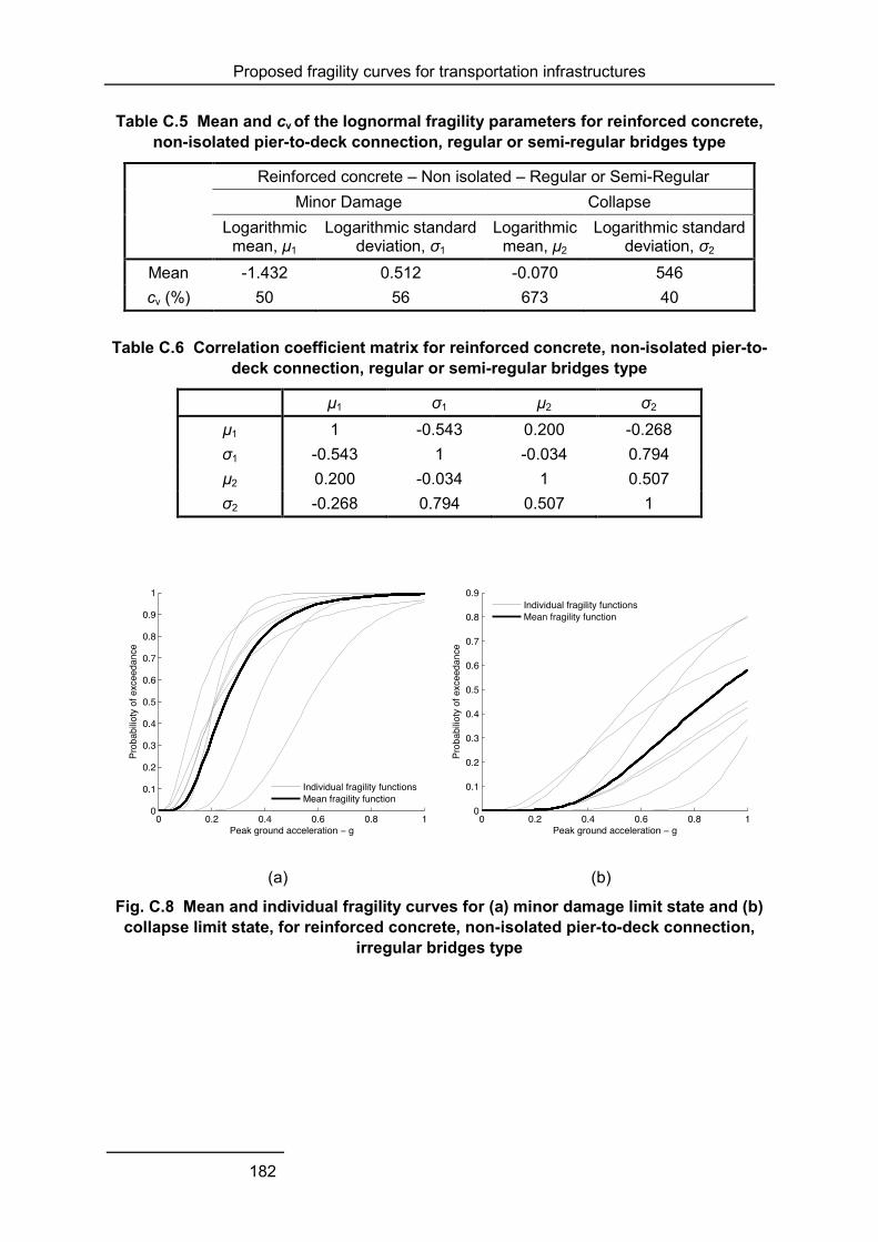
Proposed fragility curves for transportation infrastructures
182
Table C.5 Mean and cv of the lognormal fragility parameters for reinforced concrete, non-isolated pier-to-deck connection, regular or semi-regular bridges type
Reinforced concrete – Non isolated – Regular or Semi-Regular Minor Damage Collapse Logarithmic
mean, μ1 Logarithmic standard
deviation, σ1 Logarithmic
mean, μ2 Logarithmic standard
deviation, σ2 Mean -1.432 0.512 -0.070 546 cv (%) 50 56 673 40
Table C.6 Correlation coefficient matrix for reinforced concrete, non-isolated pier-to-deck connection, regular or semi-regular bridges type
μ1 σ1 μ2 σ2 μ1 1 -0.543 0.200 -0.268 σ1 -0.543 1 -0.034 0.794 μ2 0.200 -0.034 1 0.507 σ2 -0.268 0.794 0.507 1
(a) (b)
Fig. C.8 Mean and individual fragility curves for (a) minor damage limit state and (b) collapse limit state, for reinforced concrete, non-isolated pier-to-deck connection,
irregular bridges type
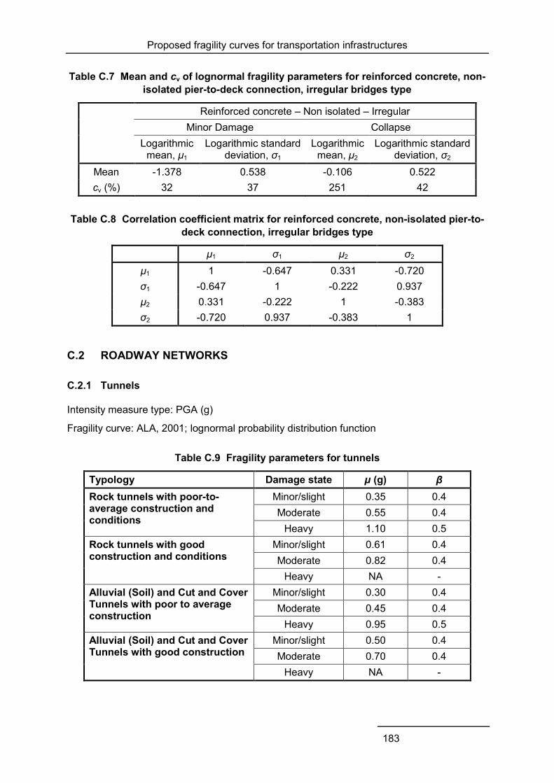
Proposed fragility curves for transportation infrastructures
183
Table C.7 Mean and cv of lognormal fragility parameters for reinforced concrete, non-isolated pier-to-deck connection, irregular bridges type
Reinforced concrete – Non isolated – Irregular Minor Damage Collapse Logarithmic
mean, μ1 Logarithmic standard
deviation, σ1 Logarithmic
mean, μ2 Logarithmic standard
deviation, σ2 Mean -1.378 0.538 -0.106 0.522 cv (%) 32 37 251 42
Table C.8 Correlation coefficient matrix for reinforced concrete, non-isolated pier-to-deck connection, irregular bridges type
μ1 σ1 μ2 σ2 μ1 1 -0.647 0.331 -0.720 σ1 -0.647 1 -0.222 0.937 μ2 0.331 -0.222 1 -0.383 σ2 -0.720 0.937 -0.383 1
C.2 ROADWAY NETWORKS
C.2.1 Tunnels
Intensity measure type: PGA (g)
Fragility curve: ALA, 2001; lognormal probability distribution function
Table C.9 Fragility parameters for tunnels
Typology Damage state µ (g) β Rock tunnels with poor-to-average construction and conditions
Minor/slight 0.35 0.4 Moderate 0.55 0.4
Heavy 1.10 0.5 Rock tunnels with good construction and conditions
Minor/slight 0.61 0.4 Moderate 0.82 0.4
Heavy NA - Alluvial (Soil) and Cut and Cover Tunnels with poor to average construction
Minor/slight 0.30 0.4 Moderate 0.45 0.4
Heavy 0.95 0.5 Alluvial (Soil) and Cut and Cover Tunnels with good construction
Minor/slight 0.50 0.4 Moderate 0.70 0.4
Heavy NA -
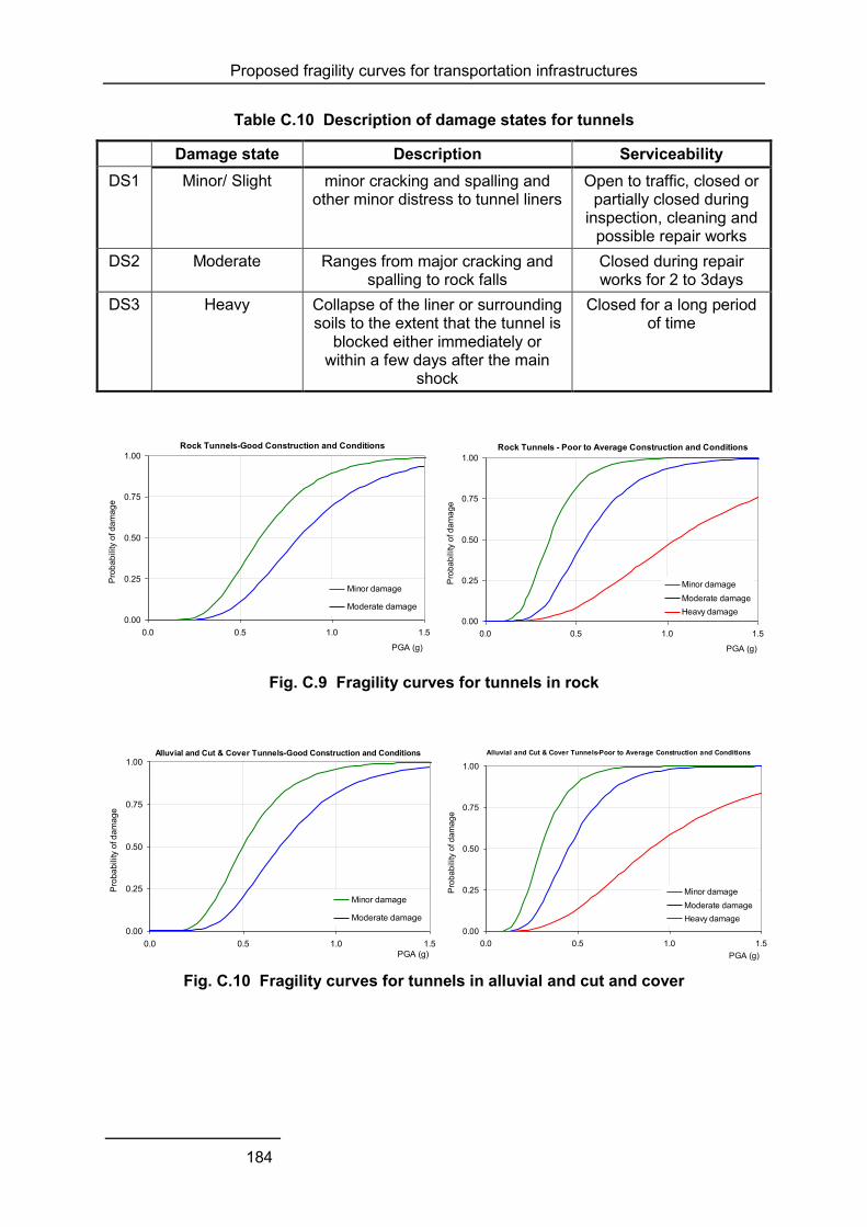
Proposed fragility curves for transportation infrastructures
184
Table C.10 Description of damage states for tunnels
Damage state Description Serviceability DS1 Minor/ Slight minor cracking and spalling and
other minor distress to tunnel liners Open to traffic, closed or
partially closed during inspection, cleaning and
possible repair works DS2 Moderate Ranges from major cracking and
spalling to rock falls Closed during repair works for 2 to 3days
DS3 Heavy Collapse of the liner or surrounding soils to the extent that the tunnel is
blocked either immediately or within a few days after the main
shock
Closed for a long period of time
Fig. C.9 Fragility curves for tunnels in rock
Fig. C.10 Fragility curves for tunnels in alluvial and cut and cover
Rock Tunnels-Good Construction and Conditions
0.00
0.25
0.50
0.75
1.00
0.0 0.5 1.0 1.5
PGA (g)
Pro
babi
lity
of d
amag
e .
Minor damage
Moderate damage
Rock Tunnels - Poor to Average Construction and Conditions
0.00
0.25
0.50
0.75
1.00
0.0 0.5 1.0 1.5
PGA (g)
Pro
babi
lity
of d
amag
e .
Minor damageModerate damageHeavy damage
Alluvial and Cut & Cover Tunnels-Good Construction and Conditions
0.00
0.25
0.50
0.75
1.00
0.0 0.5 1.0 1.5PGA (g)
Pro
babi
lity
of d
amag
e .
Minor damage
Moderate damage
Alluvial and Cut & Cover Tunnels-Poor to Average Construction and Conditions
0.00
0.25
0.50
0.75
1.00
0.0 0.5 1.0 1.5PGA (g)
Pro
babi
lity
of d
amag
e .
Minor damageModerate damageHeavy damage
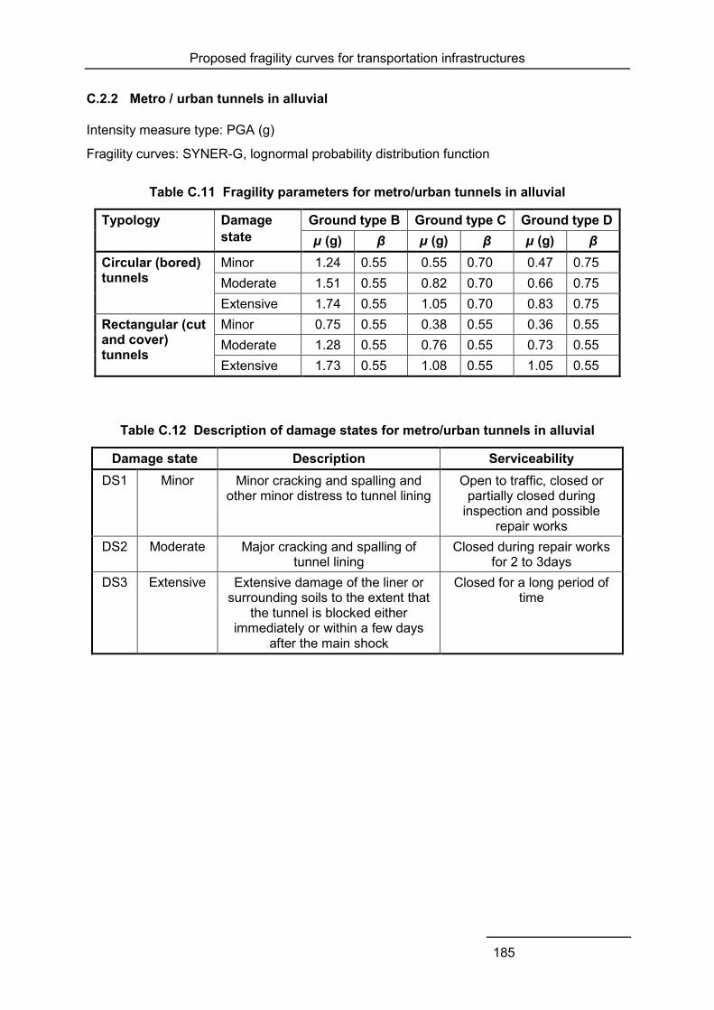
Proposed fragility curves for transportation infrastructures
185
C.2.2 Metro / urban tunnels in alluvial
Intensity measure type: PGA (g)
Fragility curves: SYNER-G, lognormal probability distribution function
Table C.11 Fragility parameters for metro/urban tunnels in alluvial
Typology Damage state
Ground type B Ground type C Ground type D µ (g) β µ (g) β µ (g) β
Circular (bored) tunnels
Minor 1.24 0.55 0.55 0.70 0.47 0.75 Moderate 1.51 0.55 0.82 0.70 0.66 0.75 Extensive 1.74 0.55 1.05 0.70 0.83 0.75
Rectangular (cut and cover) tunnels
Minor 0.75 0.55 0.38 0.55 0.36 0.55 Moderate 1.28 0.55 0.76 0.55 0.73 0.55 Extensive 1.73 0.55 1.08 0.55 1.05 0.55
Table C.12 Description of damage states for metro/urban tunnels in alluvial
Damage state Description Serviceability DS1 Minor Minor cracking and spalling and
other minor distress to tunnel lining Open to traffic, closed or
partially closed during inspection and possible
repair works DS2 Moderate Major cracking and spalling of
tunnel lining Closed during repair works
for 2 to 3days DS3 Extensive Extensive damage of the liner or
surrounding soils to the extent that the tunnel is blocked either
immediately or within a few days after the main shock
Closed for a long period of time

Proposed fragility curves for transportation infrastructures
186
Fig. C.11 Fragility curves for circular (bored) metro/urban tunnel section
Fig. C.12 Fragility curves for rectangular (cut and cover) metro/urban tunnel section
0.00
0.25
0.50
0.75
1.00
0.0 0.2 0.4 0.6 0.8 1.0 1.2 1.4 1.6
Exc
eeda
nce
Pro
babi
lity
PGA (g)
Alluvial Bored Tunnels-Soil B (EC8)
Minor damageModerate damageExtensive Damage
0.00
0.25
0.50
0.75
1.00
0.0 0.2 0.4 0.6 0.8 1.0 1.2 1.4 1.6
Exc
eeda
nce
Pro
babi
lity
PGA (g)
Alluvial Bored Tunnels-Soil C (EC8)
Minor damageModerate damageExtensive damage
0.00
0.25
0.50
0.75
1.00
0.0 0.2 0.4 0.6 0.8 1.0 1.2 1.4 1.6
Exc
eeda
nce
Pro
babi
lity
PGA (g)
Alluvial Bored Tunnels-Soil D (EC8)
Minor damageModerate damageExtensive damage
0.00
0.25
0.50
0.75
1.00
0.0 0.2 0.4 0.6 0.8 1.0 1.2 1.4 1.6
Exce
edan
ce P
roba
bilit
y
PGA (g)
Alluvial Cut & Cover Tunnels-Soil B (EC8)
Minor damageModerate damageExtensive damage
0.00
0.25
0.50
0.75
1.00
0.0 0.2 0.4 0.6 0.8 1.0 1.2 1.4 1.6
Exc
eeda
nce
Pro
babi
lity
PGA (g)
Alluvial Cut & Cover Tunnels-Soil C (EC8)
Minor damageModerate damageExtensive damage
0.00
0.25
0.50
0.75
1.00
0.0 0.2 0.4 0.6 0.8 1.0 1.2 1.4 1.6
Exc
eeda
nce
Pro
babi
lity
PGA (g)
Alluvial Cut & Cover Tunnels-Soil D (EC8)
Minor damageModerate damageExtensive damage
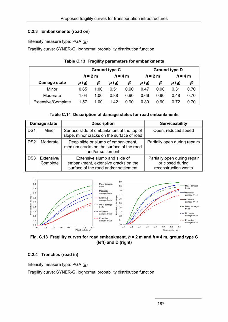
Proposed fragility curves for transportation infrastructures
187
C.2.3 Embankments (road on)
Intensity measure type: PGA (g)
Fragility curve: SYNER-G, lognormal probability distribution function
Table C.13 Fragility parameters for embankments
Ground type C Ground type D h = 2 m h = 4 m h = 2 m h = 4 m
Damage state µ (g) β µ (g) β µ (g) β µ (g) β Minor 0.65 1.00 0.51 0.90 0.47 0.90 0.31 0.70
Moderate 1.04 1.00 0.88 0.90 0.66 0.90 0.48 0.70 Extensive/Complete 1.57 1.00 1.42 0.90 0.89 0.90 0.72 0.70
Table C.14 Description of damage states for road embankments
Damage state Description Serviceability DS1 Minor Surface slide of embankment at the top of
slope, minor cracks on the surface of road Open, reduced speed
DS2 Moderate Deep slide or slump of embankment, medium cracks on the surface of the road
and/or settlement
Partially open during repairs
DS3 Extensive/ Complete
Extensive slump and slide of embankment, extensive cracks on the surface of the road and/or settlement
Partially open during repair or closed during
reconstruction works
Fig. C.13 Fragility curves for road embankment, h = 2 m and h = 4 m, ground type C
(left) and D (right)
C.2.4 Trenches (road in)
Intensity measure type: PGA (g)
Fragility curve: SYNER-G, lognormal probability distribution function
0.0
0.1
0.2
0.3
0.4
0.5
0.6
0.7
0.8
0.9
1.0
0.0 0.2 0.4 0.6 0.8 1.0 1.2 1.4
Pro
babi
lity
of d
amag
e
PGA free field (g)
Minor damage-h=4m
Moderatedamage-h=4m
Extensivedamage-h=4m
Minor damage-h=2m
Moderatedamage-h=2m
Extensivedamage-h=2m
0.0
0.1
0.2
0.3
0.4
0.5
0.6
0.7
0.8
0.9
1.0
0.0 0.2 0.4 0.6 0.8 1.0 1.2 1.4
Prob
abilit
y of
dam
age
PGA free field (g)
Minor damage-h=4m
Moderatedamage-h=4m
Extensivedamage-h=4m
Minor damage-h=2m
Moderatedamage-h=2m
Extensivedamage-h=2m

Proposed fragility curves for transportation infrastructures
188
Table C.15 Fragility parameters for road trenches
Ground type C Ground type D h = 6 m h = 4 m h = 6 m
Damage state µ (g) β µ (g) β µ (g) β Minor 0.59 1.00 0.44 1.00 0.38 1.00
Moderate 1.09 1.00 0.92 1.00 0.77 1.00 Extensive/Complete 1.90 1.00 1.77 1.00 1.46 1.00
Table C.16 Description of damage states for road trenches
Damage state Description Serviceability DS1 Minor Surface slide, minor cracks on the
surface of road Open, reduced speed
DS2 Moderate Deep slide or slump, medium cracks on the surface of the road and/or
settlement
Partially open during repairs
DS3 Extensive/ Complete
Extensive slump and slide, extensive cracks on the surface of
the road and/or settlement
Partially open or closed during repairs/reconstruction
Fig. C.14 Fragility curves for road trench, ground type C (left) and D (right)
0.0
0.1
0.2
0.3
0.4
0.5
0.6
0.7
0.8
0.9
1.0
0.0 0.2 0.4 0.6 0.8 1.0 1.2 1.4
Pro
babi
lity
of d
amag
e
PGA free field (g)
Minor damage-h=6.0m
Moderatedamage-h=6.0m
Extensivedamage-h=6.0m
0.0
0.1
0.2
0.3
0.4
0.5
0.6
0.7
0.8
0.9
1.0
0.0 0.2 0.4 0.6 0.8 1.0 1.2 1.4
Prob
abilit
y of
dam
age
PGA free field (g)
Minor damage-h=4.0m
Moderatedamage-h=4.0m
Extensivedamage-h=4.0m
Minor damage-h=6.0m
Moderatedamage-h=6.0m
Extensivedamage-h=6.0m
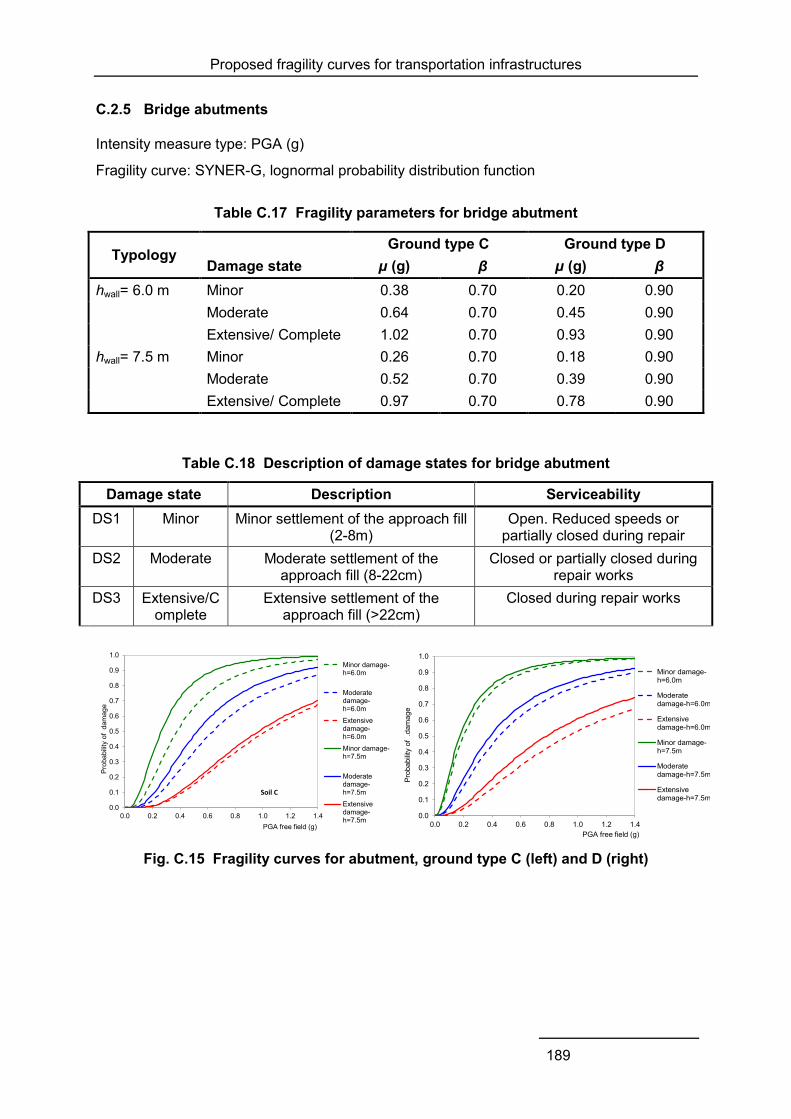
Proposed fragility curves for transportation infrastructures
189
C.2.5 Bridge abutments
Intensity measure type: PGA (g)
Fragility curve: SYNER-G, lognormal probability distribution function
Table C.17 Fragility parameters for bridge abutment
Typology Ground type C Ground type D Damage state µ (g) β µ (g) β
hwall= 6.0 m Minor 0.38 0.70 0.20 0.90 Moderate 0.64 0.70 0.45 0.90 Extensive/ Complete 1.02 0.70 0.93 0.90
hwall= 7.5 m Minor 0.26 0.70 0.18 0.90 Moderate 0.52 0.70 0.39 0.90 Extensive/ Complete 0.97 0.70 0.78 0.90
Table C.18 Description of damage states for bridge abutment
Damage state Description Serviceability DS1 Minor Minor settlement of the approach fill
(2-8m) Open. Reduced speeds or
partially closed during repair DS2 Moderate Moderate settlement of the
approach fill (8-22cm) Closed or partially closed during
repair works DS3 Extensive/C
omplete Extensive settlement of the
approach fill (>22cm) Closed during repair works
Fig. C.15 Fragility curves for abutment, ground type C (left) and D (right)
0.0
0.1
0.2
0.3
0.4
0.5
0.6
0.7
0.8
0.9
1.0
0.0 0.2 0.4 0.6 0.8 1.0 1.2 1.4
Prob
abilit
y of
dam
age
PGA free field (g)
Minor damage-h=6.0m
Moderatedamage-h=6.0m
Extensivedamage-h=6.0m
Minor damage-h=7.5m
Moderatedamage-h=7.5m
Extensivedamage-h=7.5m
Soil C
0.0
0.1
0.2
0.3
0.4
0.5
0.6
0.7
0.8
0.9
1.0
0.0 0.2 0.4 0.6 0.8 1.0 1.2 1.4
Prob
abilit
y of
.da
mag
e
PGA free field (g)
Minor damage-h=6.0m
Moderatedamage-h=6.0m
Extensivedamage-h=6.0m
Minor damage-h=7.5m
Moderatedamage-h=7.5m
Extensivedamage-h=7.5m

Proposed fragility curves for transportation infrastructures
190
C.2.6 Slopes (road on)
Intensity measure type: PGA (g)
Fragility curve: SAFELAND/SYNER-G, lognormal probability distribution function
Table C.19 Fragility parameters for roads on slopes
Damage state ky=0.05 ky=0.1 ky=0.2 ky=0.3
µ (g) β µ (g) β µ (g) β µ (g) β Minor 0.14 0.40 0.25 0.35 0.45 0.35 0.64 0.30 Moderate 0.22 0.40 0.40 0.35 0.71 0.35 1.00 0.30 Extensive/ Complete 0.37 0.40 0.64 0.35 1.11 0.35 1.55 0.30
Fig. C.16 Fragility curves at various damage states and different yield coefficients
(ky) for roads on slope
0.0
0.1
0.2
0.3
0.4
0.5
0.6
0.7
0.8
0.9
1.0
0.0 0.2 0.4 0.6 0.8 1.0 1.2 1.4 1.6 1.8 2.0
Pro
babi
lity
PGA (g)
Road on slope - Minor damage state
ky=0.05
ky=0.1
ky=0.2
ky=0.3
0.0
0.1
0.2
0.3
0.4
0.5
0.6
0.7
0.8
0.9
1.0
0.0 0.2 0.4 0.6 0.8 1.0 1.2 1.4 1.6 1.8 2.0
Pro
babi
lity
PGA (g)
Road on slope - Moderate damage state
ky=0.05
ky=0.1
ky=0.2
ky=0.3
0.0
0.1
0.2
0.3
0.4
0.5
0.6
0.7
0.8
0.9
1.0
0.0 0.2 0.4 0.6 0.8 1.0 1.2 1.4 1.6 1.8 2.0
Prob
abilit
y
PGA (g)
Road on slope - Extensive/Complete damage state
ky=0.05
ky=0.1
ky=0.2
ky=0.3
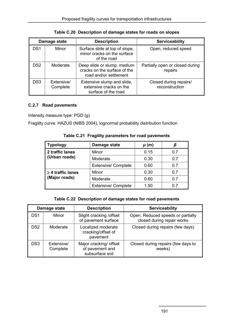
Proposed fragility curves for transportation infrastructures
191
Table C.20 Description of damage states for roads on slopes
Damage state Description Serviceability DS1 Minor Surface slide at top of slope,
minor cracks on the surface of the road
Open, reduced speed
DS2 Moderate Deep slide or slump, medium cracks on the surface of the
road and/or settlement
Partially open or closed during repairs
DS3 Extensive/ Complete
Extensive slump and slide, extensive cracks on the
surface of the road
Closed during repairs/ reconstruction
C.2.7 Road pavements
Intensity measure type: PGD (g)
Fragility curve: HAZUS (NIBS 2004), lognormal probability distribution function
Table C.21 Fragility parameters for road pavements
Typology Damage state µ (m) β 2 traffic lanes (Urban roads)
Minor 0.15 0.7 Moderate 0.30 0.7 Extensive/ Complete 0.60 0.7
4 traffic lanes (Major roads)
Minor 0.30 0.7 Moderate 0.60 0.7 Extensive/ Complete 1.50 0.7
Table C.22 Description of damage states for road pavements
Damage state Description Serviceability DS1 Minor Slight cracking /offset
of pavement surface Open. Reduced speeds or partially
closed during repair works DS2 Moderate Localized moderate
cracking/offset of pavement
Closed during repairs (few days)
DS3 Extensive/ Complete
Major cracking/ offset of pavement and subsurface soil
Closed during repairs (few days to weeks)
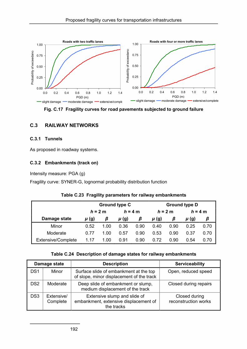
Proposed fragility curves for transportation infrastructures
192
Fig. C.17 Fragility curves for road pavements subjected to ground failure
C.3 RAILWAY NETWORKS
C.3.1 Tunnels
As proposed in roadway systems.
C.3.2 Embankments (track on)
Intensity measure: PGA (g)
Fragility curve: SYNER-G, lognormal probability distribution function
Table C.23 Fragility parameters for railway embankments
Ground type C Ground type D h = 2 m h = 4 m h = 2 m h = 4 m
Damage state µ (g) β µ (g) β µ (g) β µ (g) β Minor 0.52 1.00 0.36 0.90 0.40 0.90 0.25 0.70
Moderate 0.77 1.00 0.57 0.90 0.53 0.90 0.37 0.70 Extensive/Complete 1.17 1.00 0.91 0.90 0.72 0.90 0.54 0.70
Table C.24 Description of damage states for railway embankments
Damage state Description Serviceability DS1 Minor Surface slide of embankment at the top
of slope, minor displacement of the track Open, reduced speed
DS2 Moderate Deep slide of embankment or slump, medium displacement of the track
Closed during repairs
DS3 Extensive/ Complete
Extensive slump and slide of embankment, extensive displacement of
the tracks
Closed during reconstruction works
Roads with two traffic lanes
0.00
0.25
0.50
0.75
1.00
0.0 0.2 0.4 0.6 0.8 1.0 1.2 1.4
PGD (m)
Pro
ba
bility o
f e
xce
ed
an
ce
slight damage moderate damage extensive/complete
Roads with four or more traffic lanes
0.00
0.25
0.50
0.75
1.00
0.0 0.2 0.4 0.6 0.8 1.0 1.2 1.4
PGD (m)
Pro
ba
bility o
f e
xce
ed
an
ce
slight damage moderate damage extensive/complete
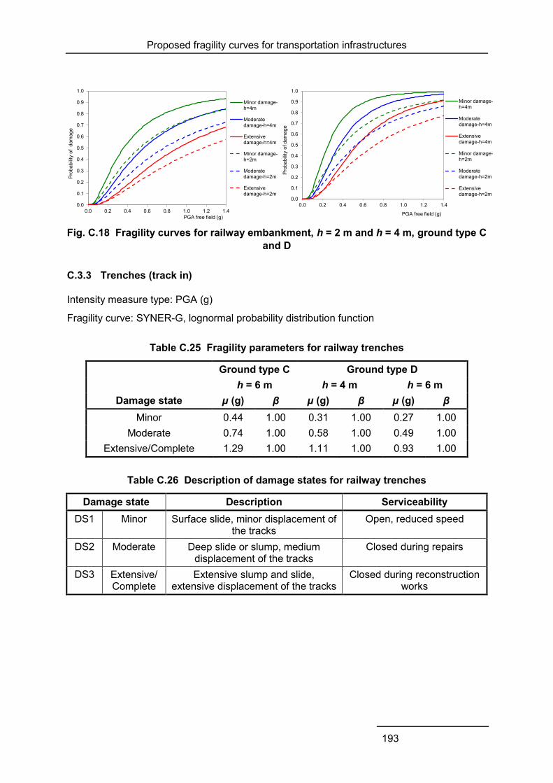
Proposed fragility curves for transportation infrastructures
193
Fig. C.18 Fragility curves for railway embankment, h = 2 m and h = 4 m, ground type C and D
C.3.3 Trenches (track in)
Intensity measure type: PGA (g)
Fragility curve: SYNER-G, lognormal probability distribution function
Table C.25 Fragility parameters for railway trenches
Ground type C Ground type D h = 6 m h = 4 m h = 6 m
Damage state µ (g) β µ (g) β µ (g) β Minor 0.44 1.00 0.31 1.00 0.27 1.00
Moderate 0.74 1.00 0.58 1.00 0.49 1.00 Extensive/Complete 1.29 1.00 1.11 1.00 0.93 1.00
Table C.26 Description of damage states for railway trenches
Damage state Description Serviceability DS1 Minor Surface slide, minor displacement of
the tracks Open, reduced speed
DS2 Moderate Deep slide or slump, medium displacement of the tracks
Closed during repairs
DS3 Extensive/ Complete
Extensive slump and slide, extensive displacement of the tracks
Closed during reconstruction works
0.0
0.1
0.2
0.3
0.4
0.5
0.6
0.7
0.8
0.9
1.0
0.0 0.2 0.4 0.6 0.8 1.0 1.2 1.4
Pro
babi
lity
of d
amag
e
PGA free field (g)
Minor damage-h=4m
Moderatedamage-h=4m
Extensivedamage-h=4m
Minor damage-h=2m
Moderatedamage-h=2m
Extensivedamage-h=2m
0.0
0.1
0.2
0.3
0.4
0.5
0.6
0.7
0.8
0.9
1.0
0.0 0.2 0.4 0.6 0.8 1.0 1.2 1.4
Prob
abilit
y of
dam
age
PGA free field (g)
Minor damage-h=4m
Moderatedamage-h=4m
Extensivedamage-h=4m
Minor damage-h=2m
Moderatedamage-h=2m
Extensivedamage-h=2m
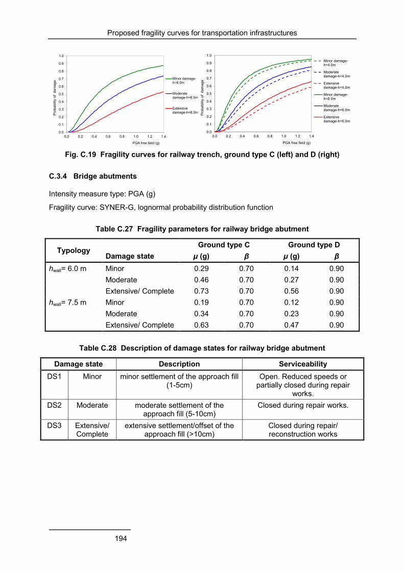
Proposed fragility curves for transportation infrastructures
194
Fig. C.19 Fragility curves for railway trench, ground type C (left) and D (right)
C.3.4 Bridge abutments
Intensity measure type: PGA (g)
Fragility curve: SYNER-G, lognormal probability distribution function
Table C.27 Fragility parameters for railway bridge abutment
Typology Ground type C Ground type D Damage state µ (g) β µ (g) β
hwall= 6.0 m Minor 0.29 0.70 0.14 0.90 Moderate 0.46 0.70 0.27 0.90 Extensive/ Complete 0.73 0.70 0.56 0.90
hwall= 7.5 m Minor 0.19 0.70 0.12 0.90 Moderate 0.34 0.70 0.23 0.90 Extensive/ Complete 0.63 0.70 0.47 0.90
Table C.28 Description of damage states for railway bridge abutment
Damage state Description Serviceability DS1 Minor minor settlement of the approach fill
(1-5cm) Open. Reduced speeds or
partially closed during repair works.
DS2 Moderate moderate settlement of the approach fill (5-10cm)
Closed during repair works.
DS3 Extensive/ Complete
extensive settlement/offset of the approach fill (>10cm)
Closed during repair/ reconstruction works
0.0
0.1
0.2
0.3
0.4
0.5
0.6
0.7
0.8
0.9
1.0
0.0 0.2 0.4 0.6 0.8 1.0 1.2 1.4
Pro
babi
lity
of d
amag
e
PGA free field (g)
Minor damage-h=6.0m
Moderatedamage-h=6.0m
Extensivedamage-h=6.0m
0.0
0.1
0.2
0.3
0.4
0.5
0.6
0.7
0.8
0.9
1.0
0.0 0.2 0.4 0.6 0.8 1.0 1.2 1.4
Prob
abilit
y of
dam
age
PGA free field (g)
Minor damage-h=4.0m
Moderatedamage-h=4.0m
Extensivedamage-h=4.0m
Minor damage-h=6.0m
Moderatedamage-h=6.0m
Extensivedamage-h=6.0m

Proposed fragility curves for transportation infrastructures
195
Fig. C.20 Fragility curves for railway abutment, ground type C (left) and D (right)
C.3.5 Slopes (track on)
Intensity measure type: PGA (g)
Fragility curve: SAFELAND/SYNER-G, lognormal probability distribution function
Fig. C.21 Fragility curves at various damage states and different yield coefficients (ky)
for railway tracks on slope
0.0
0.1
0.2
0.3
0.4
0.5
0.6
0.7
0.8
0.9
1.0
0.0 0.2 0.4 0.6 0.8 1.0 1.2 1.4
Prob
abilit
y of
dam
age
PGA free field (g)
Minor damage-h=6.0m
Moderatedamage-h=6.0m
Extensivedamage-h=6.0m
Minor damage-h=7.5m
Moderatedamage-h=7.5m
Extensivedamage-h=7.5m
0.0
0.1
0.2
0.3
0.4
0.5
0.6
0.7
0.8
0.9
1.0
0.0 0.2 0.4 0.6 0.8 1.0 1.2 1.4
Prob
abilit
y of
dam
age
PGA free field (g)
Minor damage-h=6.0m
Moderatedamage-h=6.0m
Extensivedamage-h=6.0m
Minor damage-h=7.5m
Moderatedamage-h=7.5m
Extensivedamage-h=7.5m
0.0
0.1
0.2
0.3
0.4
0.5
0.6
0.7
0.8
0.9
1.0
0.0 0.2 0.4 0.6 0.8 1.0 1.2 1.4 1.6 1.8 2.0
Prob
abili
ty
PGA (g)
Tracks on slope - Minor damage state
ky=0.05
ky=0.1
ky=0.2
ky=0.3
0.0
0.1
0.2
0.3
0.4
0.5
0.6
0.7
0.8
0.9
1.0
0.0 0.2 0.4 0.6 0.8 1.0 1.2 1.4 1.6 1.8 2.0
Prob
abili
ty
PGA (g)
Tracks on slope - Moderate damage state
ky=0.05
ky=0.1
ky=0.2
ky=0.3
0.0
0.1
0.2
0.3
0.4
0.5
0.6
0.7
0.8
0.9
1.0
0.0 0.2 0.4 0.6 0.8 1.0 1.2 1.4 1.6 1.8 2.0
Prob
abili
ty
PGA (g)
Tracks on slope - Extensive damage state
ky=0.05
ky=0.1
ky=0.2
ky=0.3

Proposed fragility curves for transportation infrastructures
196
Table C.29 Fragility parameters for railway tracks on slopes
Damage state ky=0.05 ky=0.1 ky=0.2 ky=0.3
µ (g) β µ (g) β µ (g) β µ (g) β Minor 0.11 0.60 0.20 0.60 0.37 0.60 0.52 0.60 Moderate 0.17 0.60 0.30 0.60 0.54 0.60 0.78 0.60 Extensive/ Complete 0.26 0.60 0.45 0.60 0.80 0.60 1.13 0.60
Table C.30 Description of damage states for railway tracks on slopes
Damage state Description Serviceability DS1 Minor Surface slide at top of slope,
minor displacement of the track Open, reduced speed
DS2 Moderate Deep slide or slump, medium displacement of the track
Closed during repairs
DS3 Extensive/ Complete
Extensive slump and slide, extensive displacement of the
track
Closed during reconstruction works
C.3.6 Railway tracks
Intensity measure type: PGD (g)
Fragility curve: SYNER-G, lognormal probability distribution function
Table C.31 Fragility parameters for railway tracks
Damage state µ (m) β Minor 0.03 0.70 Moderate 0.08 0.70 Extensive/ Complete 0.20 0.70
Table C.32 Description of damage states for railway tracks
Damage state Description Serviceability DS1 Minor Minor (localized) derailment
due to slight differential settlement of embankment or
offset of the ground.
Operational after inspection or short repairs.
DS2 Moderate Considerable derailment due to differential settlement or
offset of the ground.
Closed to traffic. Local repairs or replacement of tracks is
required. DS3 Extensive/
Complete Major differential settlement of
the ground resulting in potential derailment over
extended length.
Closed to traffic. Replacement of track‘s segments is required. Duration of closure depends on
length of damaged lines.

Proposed fragility curves for transportation infrastructures
197
Fig. C.22 Fragility curves for railway tracks subjected to ground failure
C.4 HARBOUR ELEMENTS
C.4.1 Waterfront structures
Intensity measure type: PGD (m)
Fragility curve: HAZUS (NIBS, 2004), lognormal probability distribution function
Table C.33 Fragility parameters for waterfront structures subject to ground failure
Damage state μ (m) β Minor/slight 0.13 0.50 Moderate 0.30 0.50 Extensive 0.43 0.50 Complete 1.09 0.50
Fig. C.23 Fragility curves for waterfront structures subject to ground failure
Railway tracks
0.00
0.25
0.50
0.75
1.00
0.0 0.1 0.2 0.3 0.4 0.5 0.6 0.7 0.8 0.9 1.0 1.1 1.2 1.3 1.4
PGD (m)
Pro
babili
ty o
f exceedance
slight damage
moderate damage
extensive/complete
WATERFRONT STRUCTURES
0,00
0,25
0,50
0,75
1,00
0,00 0,20 0,40 0,60 0,80 1,00PGD (m)
Pro
bab
ilit
y o
f exceed
an
ce
minor damage moderate damage extensive damage complete damage
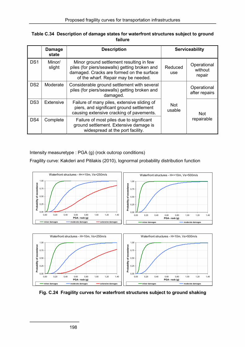
Proposed fragility curves for transportation infrastructures
198
Table C.34 Description of damage states for waterfront structures subject to ground failure
Damage state
Description Serviceability
DS1 Minor/ slight
Minor ground settlement resulting in few piles (for piers/seawalls) getting broken and damaged. Cracks are formed on the surface
of the wharf. Repair may be needed.
Reduced use
Operational without repair
DS2 Moderate Considerable ground settlement with several piles (for piers/seawalls) getting broken and
damaged.
Not usable
Operational after repairs
DS3 Extensive Failure of many piles, extensive sliding of piers, and significant ground settlement
causing extensive cracking of pavements. Not repairable DS4 Complete Failure of most piles due to significant
ground settlement. Extensive damage is widespread at the port facility.
Intensity measuretype : PGA (g) (rock outcrop conditions)
Fragility curve: Kakderi and Pitilakis (2010), lognormal probability distribution function
Fig. C.24 Fragility curves for waterfront structures subject to ground shaking
Waterfront structures - H<=10m, Vs=250m/s
0,00
0,25
0,50
0,75
1,00
0,00 0,20 0,40 0,60 0,80 1,00 1,20 1,40PGA - rock (g)
Pro
bab
ilit
y o
f exceed
an
ce
minor damages moderate damages extensive damages
Waterfront structures - H<=10m, Vs=500m/s
0,00
0,25
0,50
0,75
1,00
0,00 0,20 0,40 0,60 0,80 1,00 1,20 1,40PGA - rock (g)
Pro
bab
ilit
y o
f exceed
an
ce
minor damages moderate damages
Waterfront structures - H>10m, Vs=250m/s
0,00
0,25
0,50
0,75
1,00
0,00 0,20 0,40 0,60 0,80 1,00 1,20 1,40PGA - rock (g)
Pro
bab
ilit
y o
f exceed
an
ce
minor damages moderate damages extensive damages
Waterfront structures - H>10m, Vs=500m/s
0,00
0,25
0,50
0,75
1,00
0,00 0,20 0,40 0,60 0,80 1,00 1,20 1,40PGA - rock (g)
Pro
bab
ilit
y o
f exceed
an
ce
minor damages moderate damages
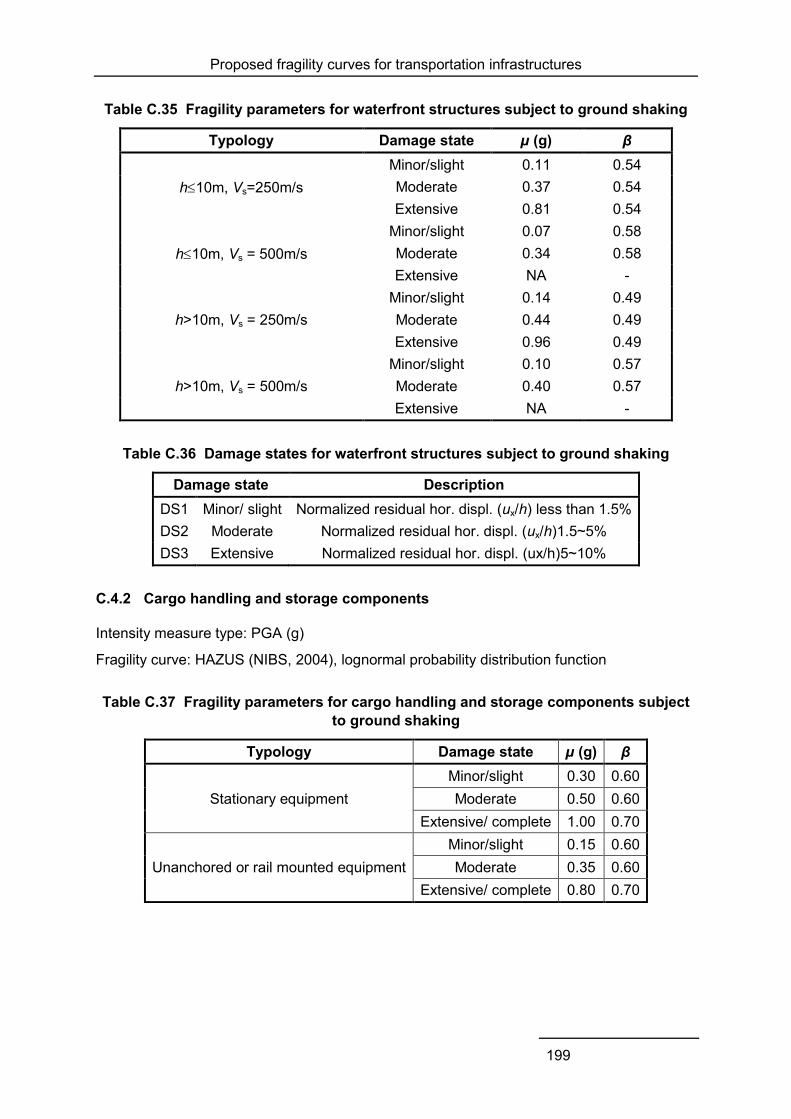
Proposed fragility curves for transportation infrastructures
199
Table C.35 Fragility parameters for waterfront structures subject to ground shaking
Typology Damage state µ (g) β
h10m, Vs=250m/s Minor/slight 0.11 0.54 Moderate 0.37 0.54 Extensive 0.81 0.54
h10m, Vs = 500m/s Minor/slight 0.07 0.58 Moderate 0.34 0.58 Extensive NA -
h>10m, Vs = 250m/s Minor/slight 0.14 0.49 Moderate 0.44 0.49 Extensive 0.96 0.49
h>10m, Vs = 500m/s Minor/slight 0.10 0.57 Moderate 0.40 0.57 Extensive NA -
Table C.36 Damage states for waterfront structures subject to ground shaking
Damage state Description DS1 Minor/ slight Normalized residual hor. displ. (ux/h) less than 1.5% DS2 Moderate Normalized residual hor. displ. (ux/h)1.5~5% DS3 Extensive Normalized residual hor. displ. (ux/h)5~10%
C.4.2 Cargo handling and storage components
Intensity measure type: PGA (g)
Fragility curve: HAZUS (NIBS, 2004), lognormal probability distribution function
Table C.37 Fragility parameters for cargo handling and storage components subject to ground shaking
Typology Damage state µ (g) β
Stationary equipment Minor/slight 0.30 0.60 Moderate 0.50 0.60
Extensive/ complete 1.00 0.70
Unanchored or rail mounted equipment Minor/slight 0.15 0.60 Moderate 0.35 0.60
Extensive/ complete 0.80 0.70
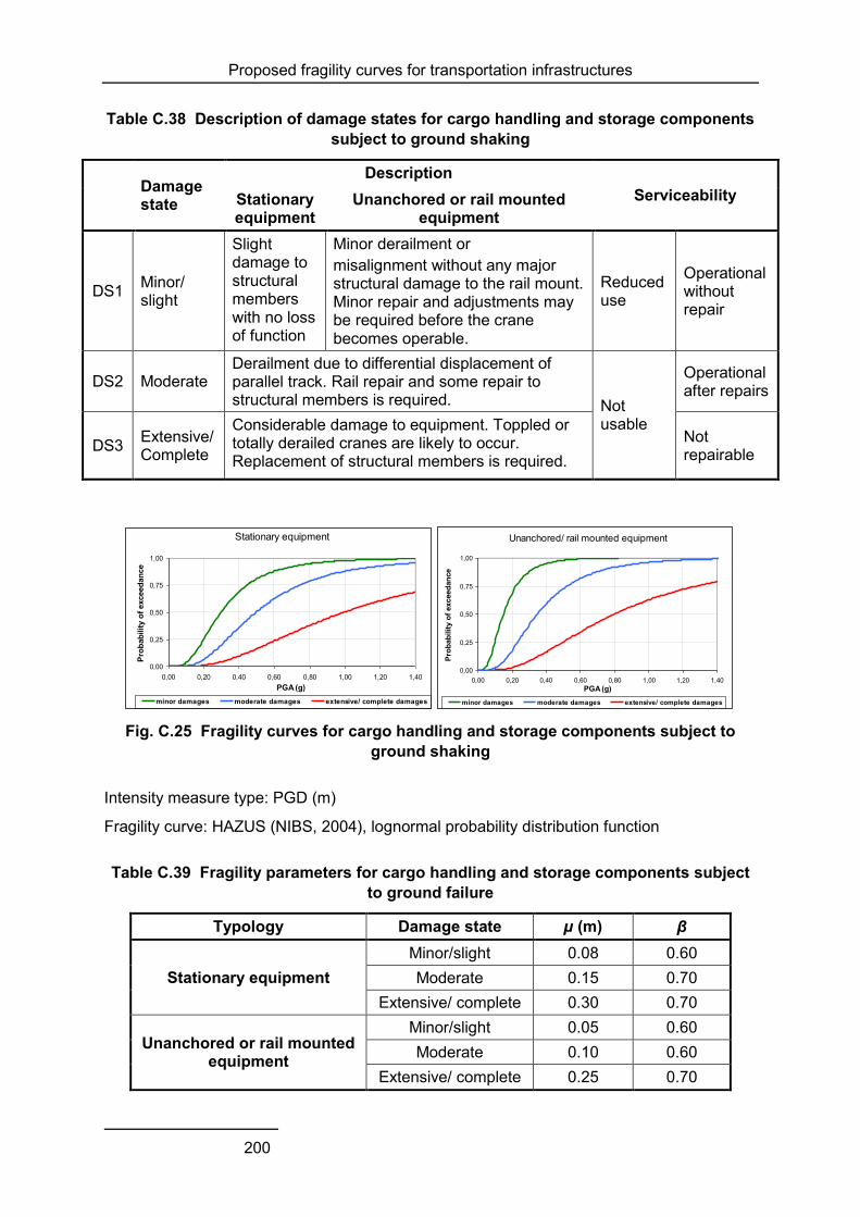
Proposed fragility curves for transportation infrastructures
200
Table C.38 Description of damage states for cargo handling and storage components subject to ground shaking
Damage state
Description Serviceability Stationary
equipment Unanchored or rail mounted
equipment
DS1 Minor/ slight
Slight damage to structural members with no loss of function
Minor derailment or misalignment without any major structural damage to the rail mount. Minor repair and adjustments may be required before the crane becomes operable.
Reduced use
Operational without repair
DS2 Moderate Derailment due to differential displacement of parallel track. Rail repair and some repair to structural members is required. Not
usable
Operational after repairs
DS3 Extensive/ Complete
Considerable damage to equipment. Toppled or totally derailed cranes are likely to occur. Replacement of structural members is required.
Not repairable
Fig. C.25 Fragility curves for cargo handling and storage components subject to
ground shaking
Intensity measure type: PGD (m)
Fragility curve: HAZUS (NIBS, 2004), lognormal probability distribution function
Table C.39 Fragility parameters for cargo handling and storage components subject to ground failure
Typology Damage state µ (m) β
Stationary equipment Minor/slight 0.08 0.60 Moderate 0.15 0.70
Extensive/ complete 0.30 0.70
Unanchored or rail mounted equipment
Minor/slight 0.05 0.60 Moderate 0.10 0.60
Extensive/ complete 0.25 0.70
Stationary equipment
0,00
0,25
0,50
0,75
1,00
0,00 0,20 0,40 0,60 0,80 1,00 1,20 1,40PGA (g)
Pro
bab
ilit
y o
f exceed
an
ce
minor damages moderate damages extensive/ complete damages
Unanchored/ rail mounted equipment
0,00
0,25
0,50
0,75
1,00
0,00 0,20 0,40 0,60 0,80 1,00 1,20 1,40PGA (g)
Pro
bab
ilit
y o
f exceed
an
ce
minor damages moderate damages extensive/ complete damages
Proposed fragility curves for transportation infrastructures
201
Fig. C.26 Fragility curves for cargo handling and storage components subject to
ground failure
Table C.40 Description of damage states for cargo handling and storage components subject to ground failure
Damage state
Description Serviceability Stationary
equipment Unanchored or rail mounted
equipment DS1
Minor/ slight
Slight damage to structural members with no loss of function
Minor derailment or misalignment without any major structural damage to the rail mount. Minor repair and adjustments may be required before the crane becomes operable.
Reduced use
Operational without repair
DS2 Moderate
Derailment due to differential displacement of parallel track. Rail repair and some repair to structural members is required.
Not usable
Operational after repairs
DS3 Extensive/ Complete
Considerable damage to equipment. Toppled or totally derailed cranes are likely to occur. Replacement of structural members is required.
Not repairable
C.4.3 Port infrastructures
For buildings, utilities and transportation networks within the harbour see the respective sections.
Liquid fuel system
Intensity measure type: PGA (g), PGD (m)
Fragility curve: SRMLIFE (2003-2007), lognormal probability distribution function
Stationary equipment
0,00
0,25
0,50
0,75
1,00
0,00 0,20 0,40 0,60 0,80 1,00PGD (m)
Pro
bab
ilit
y o
f exceed
an
ce
minor damages moderate damages extensive/ complete damages
Unanchored/ rail mounted equipment
0,00
0,25
0,50
0,75
1,00
0,00 0,20 0,40 0,60 0,80 1,00PGD (m)
Pro
bab
ilit
y o
f exceed
an
ce
minor damages moderate damages extensive/ complete damages
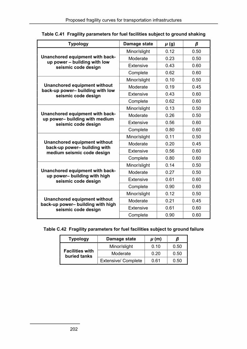
Proposed fragility curves for transportation infrastructures
202
Table C.41 Fragility parameters for fuel facilities subject to ground shaking
Typology Damage state μ (g) β
Unanchored equipment with back-up power – building with low
seismic code design
Minor/slight 0.12 0.50 Moderate 0.23 0.50 Extensive 0.43 0.60 Complete 0.62 0.60
Unanchored equipment without back-up power– building with low
seismic code design
Minor/slight 0.10 0.50 Moderate 0.19 0.45 Extensive 0.43 0.60 Complete 0.62 0.60
Unanchored equipment with back-up power– building with medium
seismic code design
Minor/slight 0.13 0.50 Moderate 0.26 0.50 Extensive 0.56 0.60 Complete 0.80 0.60
Unanchored equipment without back-up power– building with medium seismic code design
Minor/slight 0.11 0.50 Moderate 0.20 0.45 Extensive 0.56 0.60 Complete 0.80 0.60
Unanchored equipment with back-up power– building with high
seismic code design
Minor/slight 0.14 0.50 Moderate 0.27 0.50 Extensive 0.61 0.60 Complete 0.90 0.60
Unanchored equipment without back-up power– building with high
seismic code design
Minor/slight 0.12 0.50 Moderate 0.21 0.45 Extensive 0.61 0.60 Complete 0.90 0.60
Table C.42 Fragility parameters for fuel facilities subject to ground failure
Typology Damage state μ (m) β
Facilities with buried tanks
Minor/slight 0.10 0.50 Moderate 0.20 0.50
Extensive/ Complete 0.61 0.50
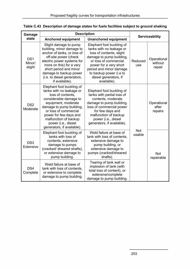
Proposed fragility curves for transportation infrastructures
203
Table C.43 Description of damage states for fuels facilities subject to ground shaking
Damage state
Description Serviceability
Anchored equipment Unanchored equipment
DS1 Minor/ slight
Slight damage to pump building, minor damage to anchor of tanks, or loss of
off-site power (check electric power systems for
more on this) for a very short period and minor
damage to backup power (i.e. to diesel generators,
if available).
Elephant foot buckling of tanks with no leakage or loss of contents, slight
damage to pump building, or loss of commercial power for a very short
period and minor damage to backup power (i.e to
diesel generators, if available).
Reduced use
Operational without repair
DS2 Moderate
Elephant foot buckling of tanks with no leakage or
loss of contents, considerable damage to
equipment, moderate damage to pump building,
or loss of commercial power for few days and malfunction of backup
power (i.e., diesel generators, if available).
Elephant foot buckling of tanks with partial loss of
contents, moderate damage to pump building, loss of commercial power
for few days and malfunction of backup
power (i.e., diesel generators, if available).
Not usable
Operational after
repairs
DS3 Extensive
Elephant foot buckling of tanks with loss of
contents, extensive damage to pumps
(cracked/ sheared shafts), or extensive damage to
pump building.
Weld failure at base of tank with loss of contents,
extensive damage to pump building, or
extensive damage to pumps (cracked/sheared
shafts). Not
repairable
DS4 Complete
Weld failure at base of tank with loss of contents, or extensive to complete
damage to pump building.
Tearing of tank wall or implosion of tank (with total loss of content), or
extensive/complete damage to pump building.
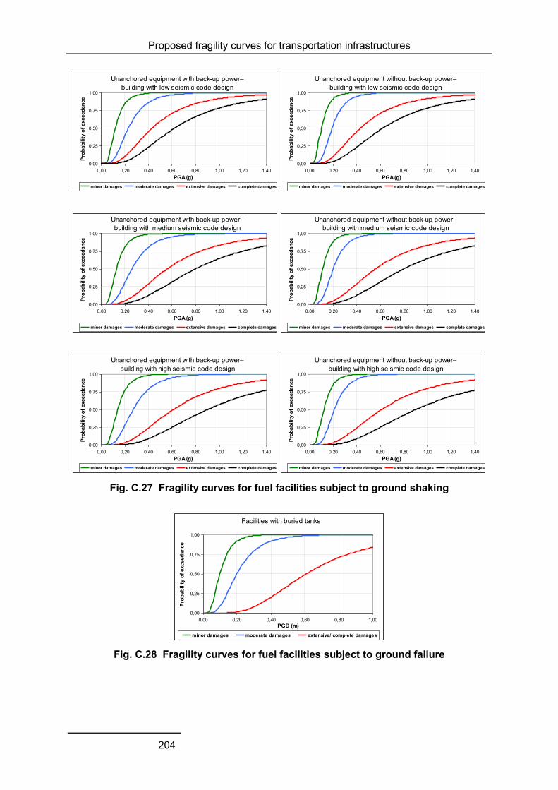
Proposed fragility curves for transportation infrastructures
204
Fig. C.27 Fragility curves for fuel facilities subject to ground shaking
Fig. C.28 Fragility curves for fuel facilities subject to ground failure
Unanchored equipment with back-up power– building with low seismic code design
0,00
0,25
0,50
0,75
1,00
0,00 0,20 0,40 0,60 0,80 1,00 1,20 1,40PGA (g)
Pro
bab
ilit
y o
f exceed
an
ce
minor damages moderate damages extensive damages complete damages
Unanchored equipment without back-up power– building with low seismic code design
0,00
0,25
0,50
0,75
1,00
0,00 0,20 0,40 0,60 0,80 1,00 1,20 1,40PGA (g)
Pro
bab
ilit
y o
f exceed
an
ce
minor damages moderate damages extensive damages complete damages
Unanchored equipment with back-up power– building with medium seismic code design
0,00
0,25
0,50
0,75
1,00
0,00 0,20 0,40 0,60 0,80 1,00 1,20 1,40PGA (g)
Pro
bab
ilit
y o
f exceed
an
ce
minor damages moderate damages extensive damages complete damages
Unanchored equipment without back-up power– building with medium seismic code design
0,00
0,25
0,50
0,75
1,00
0,00 0,20 0,40 0,60 0,80 1,00 1,20 1,40PGA (g)
Pro
bab
ilit
y o
f exceed
an
ce
minor damages moderate damages extensive damages complete damages
Unanchored equipment with back-up power– building with high seismic code design
0,00
0,25
0,50
0,75
1,00
0,00 0,20 0,40 0,60 0,80 1,00 1,20 1,40PGA (g)
Pro
bab
ilit
y o
f exceed
an
ce
minor damages moderate damages extensive damages complete damages
Unanchored equipment without back-up power– building with high seismic code design
0,00
0,25
0,50
0,75
1,00
0,00 0,20 0,40 0,60 0,80 1,00 1,20 1,40PGA (g)
Pro
bab
ilit
y o
f exceed
an
ce
minor damages moderate damages extensive damages complete damages
Facilities with buried tanks
0,00
0,25
0,50
0,75
1,00
0,00 0,20 0,40 0,60 0,80 1,00PGD (m)
Pro
bab
ilit
y o
f exceed
an
ce
minor damages moderate damages extensive/ complete damages

Proposed fragility curves for transportation infrastructures
205
Communication system
Intensity measure type: PGA(g)
Fragility curve: SRMLIFE (2003-2007), lognormal probability distribution function
Table C.44 Fragility parameters for communication facilities
Typology Damage state μ (g) β
Anchored components–low-rise building with
low seismic code design
Minor/ slight 0.30 0.55 Moderate 0.40 0.60 Extensive 0.55 0.60 Complete 0.90 0.70
Anchored components–mid-rise building with
low seismic code design
Minor/ slight 0.35 0.50 Moderate 0.45 0.45 Extensive 0.70 0.60 Complete 1.40 0.55
Anchored components–low-rise building with
high seismic code design
Minor/ slight 0.50 0.50 Moderate 0.55 0.50 Extensive 0.90 0.60 Complete 1.60 0.50
Anchored components–mid-rise building with
high seismic code design
Minor/ slight 0.35 0.55 Moderate 0.55 0.45 Extensive 0.85 0.55 Complete 1.80 0.50
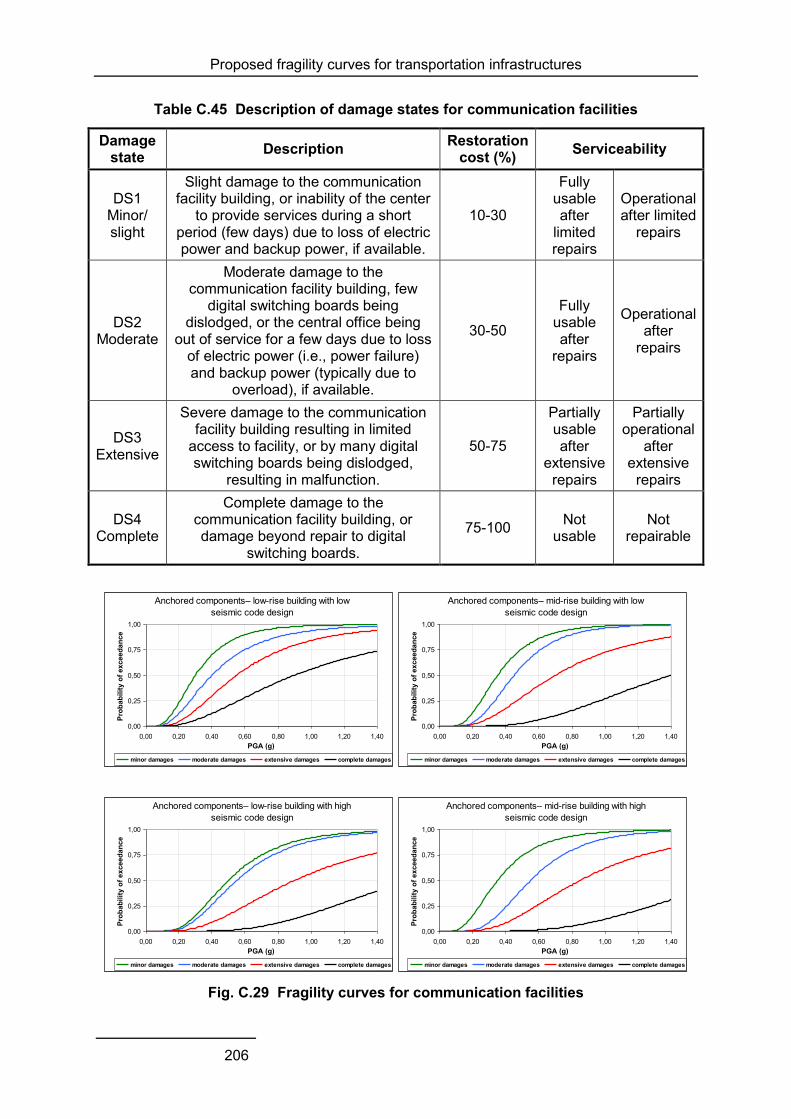
Proposed fragility curves for transportation infrastructures
206
Table C.45 Description of damage states for communication facilities
Damage state Description Restoration
cost (%) Serviceability
DS1 Minor/ slight
Slight damage to the communication facility building, or inability of the center
to provide services during a short period (few days) due to loss of electric power and backup power, if available.
10-30
Fully usable after
limited repairs
Operational after limited
repairs
DS2 Moderate
Moderate damage to the communication facility building, few
digital switching boards being dislodged, or the central office being
out of service for a few days due to loss of electric power (i.e., power failure) and backup power (typically due to
overload), if available.
30-50
Fully usable after
repairs
Operational after
repairs
DS3 Extensive
Severe damage to the communication facility building resulting in limited
access to facility, or by many digital switching boards being dislodged,
resulting in malfunction.
50-75
Partially usable after
extensive repairs
Partially operational
after extensive
repairs
DS4 Complete
Complete damage to the communication facility building, or damage beyond repair to digital
switching boards.
75-100 Not usable
Not repairable
Fig. C.29 Fragility curves for communication facilities
Anchored components– low-rise building with low seismic code design
0,00
0,25
0,50
0,75
1,00
0,00 0,20 0,40 0,60 0,80 1,00 1,20 1,40PGA (g)
Pro
bab
ilit
y o
f exceed
an
ce
minor damages moderate damages extensive damages complete damages
Anchored components– mid-rise building with low seismic code design
0,00
0,25
0,50
0,75
1,00
0,00 0,20 0,40 0,60 0,80 1,00 1,20 1,40PGA (g)
Pro
bab
ilit
y o
f exceed
an
ce
minor damages moderate damages extensive damages complete damages
Anchored components– low-rise building with high seismic code design
0,00
0,25
0,50
0,75
1,00
0,00 0,20 0,40 0,60 0,80 1,00 1,20 1,40PGA (g)
Pro
bab
ilit
y o
f exceed
an
ce
minor damages moderate damages extensive damages complete damages
Anchored components– mid-rise building with high seismic code design
0,00
0,25
0,50
0,75
1,00
0,00 0,20 0,40 0,60 0,80 1,00 1,20 1,40PGA (g)
Pro
bab
ilit
y o
f exceed
an
ce
minor damages moderate damages extensive damages complete damages
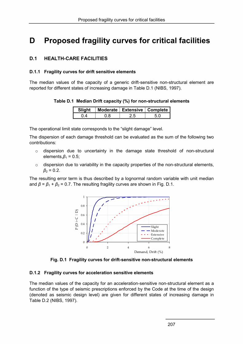
Proposed fragility curves for critical facilities
207
D Proposed fragility curves for critical facilities
D.1 HEALTH-CARE FACILITIES
D.1.1 Fragility curves for drift sensitive elements
The median values of the capacity of a generic drift-sensitive non-structural element are reported for different states of increasing damage in Table D.1 (NIBS, 1997).
Table D.1 Median Drift capacity (%) for non-structural elements
Slight Moderate Extensive Complete 0.4 0.8 2.5 5.0
The operational limit state corresponds to the “slight damage” level.
The dispersion of each damage threshold can be evaluated as the sum of the following two contributions:
o dispersion due to uncertainty in the damage state threshold of non-structural elements,β1 = 0.5;
o dispersion due to variability in the capacity properties of the non-structural elements, β2 = 0.2.
The resulting error term is thus described by a lognormal random variable with unit median and β = β1 + β2 = 0.7. The resulting fragility curves are shown in Fig. D.1.
Fig. D.1 Fragility curves for drift-sensitive non-structural elements
D.1.2 Fragility curves for acceleration sensitive elements
The median values of the capacity for an acceleration-sensitive non-structural element as a function of the type of seismic prescriptions enforced by the Code at the time of the design (denoted as seismic design level) are given for different states of increasing damage in Table D.2 (NIBS, 1997).
0
0.2
0.4
0.6
0.8
1
0 2 4 6 8
Demand, Drift (%)
P (
D >
C |
D)
Slight
Moderate
Extensive
Complete

Proposed fragility curves for critical facilities
208
Table D.2 Peak floor acceleration capacity (in g) for non-structural elements
Seismic Design Level Slight Moderate Extensive Complete High-Code 0.45 0.90 1.80 3.60
Moderate-Code 0.375 0.75 1.50 3.00 Low-Code 0.30 0.60 1.20 2.40 Pre-Code 0.30 0.60 1.20 2.40
These values have been derived for the “Special Buildings” category, characterized by increased anchorage strength of non-structural elements. For a “General Building”, where no special provisions for anchoring have been enforced, the values in Table D.2 have to be divided by a factor of 1.5.
The operational limit state corresponds to the “slight damage” level.
The dispersion of each damage threshold can be evaluated as the sum of the following two contributions:
o dispersion due to uncertainty in the damage state threshold of non-structural elements, β1 = 0.6;
o dispersion due to variability in capacity properties of the non-structural elements, β2 = 0.2.
The resulting error term is thus described by a lognormal random variable with unit median and β = β1 + β2 = 0.8.
The fragility curves for a Special Building designed according to a High-Code are shown in Fig. D.2.
Fig. D.2 Fragility curves for acceleration-sensitive non-structural elements (High-
code)
D.1.3 Fragility curves for architectural elements
The capacity parameters given in Table D.3 refer to a moderate damage state of the components, which is the level beyond which functionality of the building is compromised.
0
0.2
0.4
0.6
0.8
1
0 1 2 3 4 5
Acceleration (g)
P (
D >
C |
D)
Slight
Moderate
Extensive
Complete

Proposed fragility curves for critical facilities
209
Table D.3 Probabilistic characterisation of the capacity of the architectural elements
Object Demand Distr. Mean cv References
Walls Drift LN 0.75% 0.23 Rihal, 1982 Glazing, Doors, windows, etc.
Drift LN 4.60% 0.33 Behr and Worrell, 1998
Ceilings Acceleration LN 0.90g 0.30 Eidenger and Goettel, 1998 Badillo et al., 2003
D.1.4 Fragility curves for medical gas systems
The probabilistic description of the vulnerable components for a medical gas system is given in Table D.4.
Table D.4 Probabilistic characterisation of the capacity of the medical gas system
Object Demand Distr. Mean cv References
Cylinders Acceleration LN 0.50g 0.25 Expert judgment
Pipes Drift LN 0.90% 0.25 Kuwata and Takada, 2003
D.1.5 Fragility curves for electric power systems
The probabilistic description of the capacity of the vulnerable components is given in Table D.5.
Table D.5 Probabilistic characterisation of the capacity of the electric power system
Object Demand Distr. Mean cv References Diesel conduits Drift LN 0.90% 0.25 Kuwata and Takada, 2003 Battery cabinet Acceleration LN 0.52g 0.62 Swan and Kassawara, 1998 General switchboard panel Acceleration LN 1.12g 0.64 Swan and Kassawara, 1998
Floor distribution panel Acceleration LN 1.75g 0.68 Swan and Kassawara, 1998
D.1.6 Fragility curves for water systems
The probabilistic description of the water system capacity is given in Table D.6.
Table D.6 Probabilistic characterisation of the capacity of the water system
Object Demand Distr. Mean cv References
Piping Drift LN 0.90% 0.25 Kuwata and Takada, 2003

Proposed fragility curves for critical facilities
210
D.1.7 Fragility curves for elevators
The probabilistic model of the elevator capacity is given in Table D.7.
Table D.7 Probabilistic characterisation of the capacity of the elevator system
Object Demand Distr. Mean cv References Elevator (Global criteria) PGA LN 0.20g 0.30 Nuti et al., 1999

European Commission
EUR 25880 EN--- Joint Research Centre --- Institute for the Protection and Security of the Citizen
Title: Guidelines for deriving seismic fragility functions of elements at risk: Buildings, lifelines, transportation networks
and critical facilities
Authors: Amir M. Kaynia, Iunio Iervolino, Fabio Taucer, Ufuk Hancilar
Luxembourg: Publications Office of the European Union
2013 --- 250 pp. --- 21.0 x 29.7 cm
EUR --- Scientific and Technical Research series --- ISSN 1831-9424 (online), ISSN 1018-5593 (print)
ISBN 78-92-79-28966-8
doi:10.2788/19605
Abstract The objective of SYNER-G in regards to the fragility functions is to propose the most appropriate functions for the construction
typologies in Europe. To this end, fragility curves from literature were collected, reviewed and, where possible, validated against
observed damage and harmonised. In some cases these functions were modified and adapted, and in other cases new curves
were developed. The most appropriate fragility functions are proposed for buildings, lifelines, transportation infrastructures and
critical facilities. A software tool was also developed for the storage, harmonisation and estimation of the uncertainty of fragility
functions.

z
As the Commission’s in-house science service, the Joint Research Centre’s mission is to provide EU policies with independent, evidence-based scientific and technical support throughout the whole policy cycle. Working in close cooperation with policy Directorates-General, the JRC addresses key societal challenges while stimulating innovation through developing new standards, methods and tools, and sharing and transferring its know-how to the Member States and international community. Key policy areas include: environment and climate change; energy and transport; agriculture and food security; health and consumer protection; information society and digital agenda; safety and security including nuclear; all supported through a cross-cutting and multi-disciplinary approach.
LB-NA-25880-EN
-N