
Guidance Notes on Ice Class - American Bureau of Shipping · PDF fileThe purpose of these...
86
GUIDANCE NOTES ON ICE CLASS MARCH 2005 (Updated February 2014 – see next page) American Bureau of Shipping Incorporated by Act of Legislature of the State of New York 1862 Copyright 2005 American Bureau of Shipping ABS Plaza 16855 Northchase Drive Houston, TX 77060 USA
Transcript of Guidance Notes on Ice Class - American Bureau of Shipping · PDF fileThe purpose of these...
GUIDANCE NOTES ON
ICE CLASS
MARCH 2005 (Updated February 2014 – see next page)
American Bureau of Shipping Incorporated by Act of Legislature of the State of New York 1862
Copyright 2005 American Bureau of Shipping ABS Plaza 16855 Northchase Drive Houston, TX 77060 USA

Updates
February 2014 consolidation includes:
October 2008 version plus Corrigenda/Editorials
October 2008 consolidation includes:
March 2005 version plus Corrigenda/Editorials

ABS GUIDANCE NOTES ON ICE CLASS . 2005 i
Foreword
Foreword The purpose of these Guidance Notes is to provide ship designers with clear guidance on alternative design procedures for hull side structures, on alternative methods for determination of power requirements, and on procedures for propeller strength assessment based on the Finite Element Method for Baltic Ice Class Vessels.
• Chapter 1 provides a procedure on ice strengthening designs using direct calculation approaches.
• Chapter 2 provides a procedure for the calculation of power requirement for ice class vessels.
• Chapter 3 provides a procedure for the strength analysis of propellers for ice class vessels.
This document is referred to herein as “these Guidance Notes” and its issue date is 31 March 2005. Users of these Guidance Notes are encouraged to contact ABS with any questions or comments concerning these Guidance Notes. Users are advised to check with ABS to ensure that this version of these Guidance Notes is current.
These Guidance Notes supersede the 2004 ABS Guidance Notes on Nonlinear Finite Element Analysis of Side Structures Subject to Ice Loads.

This Page Intentionally Left Blank

ABS GUIDANCE NOTES ON ICE CLASS . 2005 iii
Table of Contents
GUIDANCE NOTES ON
ICE CLASS
CONTENTS CHAPTER 1 Ice Strengthening Using Direct Calculation Approaches ..1
Section 1 Introduction ...............................................................5 Section 2 Procedure for Ice Strengthening Side Structures
Using Nonlinear FEM................................................7 Section 3 References..............................................................11 Appendix 1 Nonlinear FE Model ................................................13 Appendix 2 Example of Nonlinear FEM Applications ................21 Appendix 3 The Finnish Maritime Administration (FMA)
“Tentative Note for Application of Direct Calculation Methods for Longitudinally Framed Hull Structure”, 30 June 2003 ...................29
CHAPTER 2 Power Requirement for Ice Class .......................................33
Section 1 Introduction .............................................................35 Section 2 Alternative Methods to Calculate KC ......................37 Section 3 Alternative Methods to Determine Rch (Resistance
in Brash Ice)............................................................41 Section 4 References..............................................................45 Appendix 1 Examples ................................................................47
CHAPTER 3 Propeller Strength Assessment..........................................49
Section 1 General Design Basis .............................................51 Section 2 Ice Load Determination...........................................53 Section 3 Blade Stress Analysis Procedure ...........................61 Section 4 Summary of Propeller Strength Assessment
Procedure ...............................................................67 Section 5 References..............................................................69 Appendix 1 Illustrative Example.................................................71

This Page Intentionally Left Blank

ABS GUIDANCE NOTES ON ICE CLASS . 2005 1
Chapter 1: Ice Strengthening Using Direct Calculation Approaches
C H A P T E R 1 Ice Strengthening Using Direct Calculation Approaches
CONTENTS SECTION 1 Introduction ............................................................................5
1 Background............................................................................5 2 Purpose..................................................................................5 3 Applications............................................................................6 4 Key Components of these Guidance Notes ..........................6 5 Contents of this Chapter ........................................................6
SECTION 2 Procedure for Ice Strengthening Side Structures Using
Nonlinear FEM ........................................................................7 1 Design of Side Structures ......................................................7 2 Step 1: FSICR Design............................................................7 3 Step 2: FMA Interim Design...................................................8 4 Step 3: Alternative Design for Side Longitudinals .................8
4.1 FEM Modeling ...................................................................8 4.2 Ice Load on Side Longitudinals .........................................8 4.3 Acceptance Criteria...........................................................8
5 Step 4: Alternative Design of Side Shell ................................9 5.1 FEM Modeling ...................................................................9 5.2 Ice Load on Side Shell ......................................................9 5.3 Acceptance Criteria...........................................................9 5.4 Abrasion/Corrosion ...........................................................9
TABLE 1 Steps in Ice Strengthening of Side Structures .............7
SECTION 3 References............................................................................11 APPENDIX 1 Nonlinear FE Model..............................................................13
1 Structural Idealization ..........................................................13 1.1 Introduction .....................................................................13 1.2 Extent of Structural Modeling .......................................... 13 1.3 FEM Elements.................................................................13 1.4 Mesh Size .......................................................................14
2 Material Model .....................................................................15

2 ABS GUIDANCE NOTES ON ICE CLASS . 2005
3 Boundary Conditions............................................................15 4 Line Load on Side Longitudinals..........................................16 5 Patch Load on Side Shell Plate ...........................................17 6 FEM Solution .......................................................................18
6.1 Incremental Solution........................................................18 6.2 Convergence ...................................................................18
7 Nonlinear FEM Theory and Software ..................................18 7.1 Material Nonlinearity........................................................18 7.2 Geometrical Nonlinearity .................................................19 7.3 Incremental Solutions......................................................19 7.4 Convergence Criteria ......................................................19 7.5 Commercial FEM package ..............................................19
TABLE 1 Boundary Conditions for FE Model ............................16 FIGURE 1 FE Model Extent (Inner Skin Removed for
Clarity)........................................................................14 FIGURE 2 Mesh of Side Longitudinal and Bracket at
Connection to Web Frame.........................................15 FIGURE 3 Boundary Conditions for FE Model ............................16 FIGURE 4 Ice Load as Line Load on Side Longitudinal..............17 FIGURE 5 Ice Patch Load Applied on Side Shell Plate ..............17
APPENDIX 2 Example of Nonlinear FEM Applications ........................... 21
1 Problem Definition................................................................21 2 FEM Modeling......................................................................21 3 Ice Load ...............................................................................23 4 Analysis Results...................................................................23 5 Alternative Design................................................................25 6 Example of Alternative Side Shell Design ...........................26 FIGURE 1 FE Model....................................................................22 FIGURE 2 Load Path (Loading and Unloading Phases) .............23 FIGURE 3 Von Mises Stress Contour .........................................24 FIGURE 4 Pressure vs. Deflection (Loading and Unloading
Phases) ......................................................................25 FIGURE 5 Pressure vs. Deflection of Different Designs .............25 FIGURE 6 Deformed Side Structure – View from Outside..........26 FIGURE 7 Deformed Side Structure – View from Inside.............26 FIGURE 8 Pressure vs. Deflection of Side Shell Plate ...............27

ABS GUIDANCE NOTES ON ICE CLASS . 2005 3
APPENDIX 3 The Finnish Maritime Administration (FMA) “Tentative Note for Application of Direct Calculation Methods for Longitudinally Framed Hull Structure”, 30 June 2003......29 1 Introduction ..........................................................................29 2 Maximum frame spacing......................................................30
2.1 Plating thickness .............................................................30 2.2 Frame section modulus and shear area for longitudinal
frames .............................................................................30 3 Brackets on intersections between longitudinal frames
and the web frames .............................................................31

This Page Intentionally Left Blank

ABS GUIDANCE NOTES ON ICE CLASS . 2005 5
Section 1: Introduction
C H A P T E R 1 Ice Strengthening Using Direct Calculation Approaches
S E C T I O N 1 Introduction
1 Background According to the Finnish-Swedish Ice Class Rules (abbreviated as “FSICR” in these Guidance Notes), it is stipulated that longitudinal frames shall be attached to all supporting web frames and bulkheads by brackets. In a subsequent paragraph, it is stated that “For the formulae and values given in this section for the determination of hull scantlings, more sophisticated methods may be substituted subject to approval by the administration or the classification society.”
Ice load measurements conducted with vessels navigating in the Baltic show that loads several times higher than the design loads are often encountered. It is deemed that designing up to the yield point with these high loads would be uneconomical, and so, some excess of the nominal design load is acceptable.
In certain extreme cases, some plastic deformation will occur, leaving behind a permanent set. The design of the longitudinal frames can be checked by using a FEM program capable of nonlinear structural analysis. In such an analysis, the permanent set can be calculated and the ultimate load-carrying capacity of the frames predicted.
The Finnish Maritime Administration (abbreviated as “FMA” in these Guidance Notes) released the “Tentative Note for Application of Direct Calculation Methods for Longitudinally Framed Hull Structure” (referred to as “FMA Guidelines” in these Guidance Notes) for alternative design of side structures using nonlinear FEM analysis. See Chapter 1, Appendix 3.
In 2004, ABS released the Guidance Notes on Nonlinear Finite Element Analysis of Side Structures Subject to Ice Loads to provide a procedure to design side longitudinals using a nonlinear FEM analysis. This publication incorporates the information in the 2004 Guidance Notes and supersedes that publication.
2 Purpose The purpose of this Chapter is to clearly define a procedure for ice strengthening of side structures using nonlinear FEM, including both side longitudinals and side shell plating. In accordance with Ice Class Rules, the results of such an analysis may be used to substitute for standard Rules formulae. Certain design requirements, such as constraints on longitudinal frame spacing, the bracket attachment requirement between web frames and bulkheads and side shell thickness, may be relaxed.
These Guidance Notes provide more technical details to supplement the FMA Guidelines. In addition, these Guidance Notes provide a procedure for alternative design of side shell plate using nonlinear FEM. This may lead to relaxation of side shell plating thickness requirements compared to the FMA Guidelines.

Chapter 1 Ice Strengthening Using Direct Calculation Approaches Section 1 Introduction 1-1
6 ABS GUIDANCE NOTES ON ICE CLASS . 2005
3 Applications The requirement that the maximum frame spacing of longitudinal frames “shall not exceed 0.35 meter for ice class IA Super and IA and shall in no case exceed 0.45 meter” stems from the fact that the ice loading is concentrated along a narrow horizontal strip, typically only 250 mm wide. In order to limit the possible catastrophic consequences of longitudinal frames collapsing, there is a Rule requirement to install brackets between longitudinal frames and transverse webs. These brackets increase the ultimate load-carrying capacity of the frames by effectively reducing their span. However, the installation of such brackets may lead to higher production costs, and it is desirable to use nonlinear FEM to justify a decision to omit such brackets in order to optimize structural design.
Nonlinear FEM is also used to optimize the design with a balanced strength between side shell plate and side longitudinals.
4 Key Components of these Guidance Notes The key components of applying a nonlinear FEM analysis of side structures subject to ice loads include:
• Design procedure
• Nonlinear FE model, including structural idealization, material modeling, loading, solution, convergence requirements etc.
These analysis components can be expanded into additional topics, as follows, which become the subject of particular Sections in the remainder of this Chapter
5 Contents of this Chapter Chapter 1 of these Guidance Notes is divided into the following Sections and Appendices:
• Section 1 – Introduction
• Section 2 – Procedure for Ice Strengthening Side Structures Using Nonlinear FEM
• Appendix 1 – Nonlinear FE Model
• Appendix 2 – Example of Nonlinear FEM Applications
• Appendix 3 – The Finnish Maritime Administration (FMA) “Tentative Note for Application of Direct Calculation Methods for Longitudinally Framed Hull Structure”, 30 June 2003

ABS GUIDANCE NOTES ON ICE CLASS . 2005 7
Section 2: Procedure for Ice Strengthening Side Structures Using Nonlinear FEM
C H A P T E R 1 Ice Strengthening Using Direct Calculation Approaches
S E C T I O N 2 Procedure for Ice Strengthening Side Structures Using Nonlinear FEM
1 Design of Side Structures The ice strengthening procedure involves four steps for alternative design of the side structure under ice load. These four steps are summarized in 1-2/Table 1 and are described in detail below.
TABLE 1 Steps in Ice Strengthening of Side Structures
Step Design Notes 1 FSICR design, baseline design Design fully complies with FSICR
(Ice strengthened longitudinal spacing, less than 450 mm) 2 FMA interim design Design complies with the FMA Guidelines, item 2
(Longitudinal spacing is wider than that specified by FSICR) 3 Alternative design for side longitudinals Side longitudinals without brackets are determined using
nonlinear FEM. 4 Alternative design for side shell Side shell thickness is determined using nonlinear FEM for
extreme ice loads.
2 Step 1: FSICR Design The initial design of side structures should fully comply with FSICR. FSICR require that the maximum frame spacing of longitudinal frames “shall not exceed 0.35 meter for ice class IA Super and IA and shall in no case exceed 0.45 meter”. Brackets are required to connect longitudinals and webs.

Chapter 1 Ice Strengthening Using Direct Calculation Approaches Section 2 Procedure for Ice Strengthening Side Structures Using Nonlinear FEM 1-2
8 ABS GUIDANCE NOTES ON ICE CLASS . 2005
3 Step 2: FMA Interim Design FMA interim design uses the FMA Guidelines to design side structure with longitudinal spacing about 800 millimeters. The ice pressure is higher than that of FSICR. Brackets are needed to connect longitudinals and webs.
The side shell plating thickness is calculated following the FMA Guidelines (see Chapter 1, Appendix 3), as in the equation below:
cY
PL tf
pst +
⋅⋅⋅=
σ2667 mm
where pPL is the ice pressure acting on the side shell plating. The details of this equation can be found in the FMA Guidelines (1-A3/2.1).
4 Step 3: Alternative Design for Side Longitudinals Alternative structures shall follow the FMA Guidelines to ensure equivalency in permanent deformation of the side longitudinals. Nonlinear FEM can be applied to evaluate this equivalency. Structural modeling is to follow the procedure in these Guidance Notes. The permanent deformation of the side longitudinals should be checked by the acceptance criteria in 1-2/4.3. The details of this step, including the FEM modeling, load applied and acceptance criteria, are described below.
4.1 FEM Modeling The FEM modeling procedure and boundary condition requirements are described in Chapter 1, Appendix 1. Other details about FEM, including FEM solution and convergence requirements can also be found in Chapter 1, Appendix 1.
4.2 Ice Load on Side Longitudinals For the purpose of designing a side longitudinal and its end connections to web frames, the ice loads may be represented as line loads acting on the longitudinal within the ice belt. The load applied to the FE model is described in detail in 1-A1/4.
4.3 Acceptance Criteria FMA recommends “… that the shell structure is modeled both for the rule requirements with brackets and for the proposed structure without brackets. If the plastic deformation for the proposed structure is equal to or smaller than for the rule structure, the scantlings of the proposed structure may be considered acceptable.” (See Chapter 1, Appendix 3.)
The proposed unbracketed design is to be compared with the FMA interim design. The Finite Element procedures outlined in these Guidance Notes should be used to perform the analysis of both bracketed and unbracketed designs. If an unbracketed longitudinal scantling can be shown to resist plastic deformation such that it results in permanent deformation that is either equal to or less than the Rule bracket design, the unbracketed design can be accepted. The FSICR initial design and FMA interim design can be used as the benchmark for this comparison.
Chapter 1 Ice Strengthening Using Direct Calculation Approaches Section 2 Procedure for Ice Strengthening Side Structures Using Nonlinear FEM 1-2
ABS GUIDANCE NOTES ON ICE CLASS . 2005 9
5 Step 4: Alternative Design of Side Shell Alternative design of side shell plating thickness may also be accepted if the resulting permanent deformation of shell plating subject to extreme ice loads falls within an acceptable range. Nonlinear FEM analysis is to be performed to calculate the permanent deformation of the side shell plating. The side longitudinal is the same as the FMA alternative design as in Step 3. Permanent deformation of the side shell plating is to be checked by the acceptance criteria in 1-2/5.3 to determine the reasonable side shell thickness.
5.1 FEM Modeling The FE model is the same as the FMA alternative design in Step 3, following the same requirements in Chapter 1, Appendix 1, with the same side longitudinals. The side shell thickness may be reduced based on the thickness requirement calculated from the FMA Guidelines in Step 3. The boundary conditions and convergence requirements are the same as those in Step 3.
5.2 Ice Load on Side Shell Ice loads are to be modeled as patch loads and be applied to the side shell between supporting structures. These extreme ice loads are calculated based on the following guidelines:
• Pressure equal to 3 times the ice pressure for plating in the FMA Guideline
• Length of patch loads equals 2 times longitudinal spacing.
• Load height equals that defined in FSICR.
The load applied to the FE model is explained in 1-A1/5.
5.3 Acceptance Criteria Permanent deformation of the side shell between longitudinals up to 2% of longitudinal spacing is acceptable. However, in no case can the thickness before the abrasion/corrosion margin is added be less than 90% of the current FMA requirement, as in the FMA alternative design (Step 2).
5.4 Abrasion/Corrosion The increment for abrasion/corrosion of 2 millimeters must be applied to the side shell plate unless special treatment is applied to the hull surface. This abrasion/corrosion margin is to be added to the thickness as calculated.

This Page Intentionally Left Blank

ABS GUIDANCE NOTES ON ICE CLASS . 2005 11
Section 3: References
C H A P T E R 1 Ice Strengthening Designs Using Direct Calculation Approaches
S E C T I O N 3 References
ABS, 2004. Guidance Notes on Nonlinear Finite Element Analysis of Side Structures Subject to Ice Loads. American Bureau of Shipping, April 2004.
ABS, 2005. Rules for Building and Classing Steel Vessels. American Bureau of Shipping, 2005
FMA, 2002. Finnish-Swedish Ice Class Rules
FMA, 2003, Tentative Guidelines for Application of Direct Calculation Methods for Longitudinally Framed Hull Structure, FMA, issued 30 June 2003.
FMA, 2004, Guidelines for the Application of the Finnish-Swedish Ice Class Rules, FMA, draft 19 November 2004

This Page Intentionally Left Blank
ABS GUIDANCE NOTES ON ICE CLASS . 2005 13
Appendix 1: Ice Strengthening Designs Using Direct Calculation Approaches
C H A P T E R 1 Ice Strengthening Designs Using Direct Calculation Approaches
A P P E N D I X 1 Nonlinear FE Model
1 Structural Idealization
1.1 Introduction In order to create a three-dimensional model that can be analyzed in a reasonable amount of time, a subsection of the vessel’s side structure is considered. Indeed, as long as enough structure is modeled to sufficiently move the boundary effects of fixity away from the area of interest, there is no benefit in modeling a greater area of the vessel structure. The result on the longitudinal frame of interest will remain the same, although the analysis time could increase substantially.
1.2 Extent of Structural Modeling The three-dimensional structural model is to be justified as being representative of the behavior of side structures subject to ice loads.
i) Longitudinal direction. In principle, the structural model is to extend a minimum of three webs (three-bay model) with an extra half-frame spacing on the forward and aft ends.
ii) Vertical extent. In principle, the structural model is to extend between the two horizontal stringers that include the ice belt region. Typically, the ice belt is applied in the area of a single longitudinal frame that is halfway between the stringers. The model should contain at least one three-dimensional longitudinal frame above and below the frame of interest. Modeling more than three three-dimensional longitudinal frames will require more time for modeling and analysis with little to no appreciable difference in the result.
iii) Transverse direction. The FE model extends to and includes the inner skin.
Structures to be modeled include:
• Side shell plating and side longitudinal frames
• Web frames, web stiffeners and brackets, if any
• Inner skin plating and attached longitudinals
1.3 FEM Elements Shell elements are generally used for representing the side shell, inner skin, web frames and web and flange of the side longitudinal within the ice belt.
Beam elements can be used for side longitudinals outside of the ice belt.
The flange of the side longitudinals within the ice belt can be modeled using either shell elements or beam elements.

Chapter 1 Ice Strengthening Using Direct Calculation Approaches Appendix 1 Nonlinear FE Model 1-A1
14 ABS GUIDANCE NOTES ON ICE CLASS . 2005
1.4 Mesh Size Mesh size should be selected such that the modeled structures reasonably represent the nonlinear behavior of the structures. Areas where high local stress or large deflections are expected are to be modeled with fine meshes. 1-A1/Figure 1 shows an example of the FEM mesh.
FIGURE 1 FE Model Extent (Inner Skin Removed for Clarity)
It is preferable to use quadrilateral elements that are nearly square in shape. The aspect ratio of elements should be kept below 3-to-1.
In general, the web of a longitudinal is to be divided into at least three elements (see 1-A1/Figure 2). The flange of a side longitudinal can be modeled by one shell element or by a beam element.
The side shell, web frames and inner skin can be divided into elements that are of the same size as that for the web of side longitudinal. Structures away from the ice belt may be represented using a coarser mesh. Tapering of fine mesh to relatively coarse mesh is acceptable.
When modeling brackets, the mesh should be finer in order to carry at least three elements in the area where the bracket meets the longitudinal flange (see 1-A1/Figure 2). It is recommended to keep element edges normal to the bracket boundary and avoid using triangular-shaped elements. Also, it is preferable not to use quadrilaterals oriented in such a way that only one point touches a bracket boundary.

Chapter 1 Ice Strengthening Using Direct Calculation Approaches Appendix 1 Nonlinear FE Model 1-A1
ABS GUIDANCE NOTES ON ICE CLASS . 2005 15
FIGURE 2 Mesh of Side Longitudinal and Bracket at Connection to Web Frame
2 Material Model Material nonlinearity results from the nonlinear relationship between stress and strain once the elastic yield limit of the material has been reached. The behavior of materials beyond yield is typically characterized by the slope of the stress-strain curve that indicates the degree of hardening. In general, it is recommended to use an elastic-perfectly-plastic material model for shipbuilding steel that does not account for strain hardening effects. This simplification yields conservative results.
The elastic-perfectly-plastic material model for mild steel is characterized by the following parameters:
Yield Stress 235 MPa
Young’s Modulus (elastic) 206,000 MPa
Poisson’s Ratio 0.3
3 Boundary Conditions The boundary conditions constrain the model in space while permitting the longitudinal frame to flex as it would if the entire structure had been modeled.
1-A1/Table 1 and 1-A1/Figure 3 show the recommended boundary conditions.
• The top and bottom cut planes (ADHE and BCGF) apply complete translational fixity, but allow rotation about the vessel’s longitudinal axis. This represents the rigidity of the horizontal stringers bounding the vertical model extent.
• The forward and aft cut planes (ABCD and EFGH) apply a symmetric condition with respect to the plane perpendicular to the vessel’s longitudinal direction. This represents that the structure is continuous in the vessel’s longitudinal direction.

Chapter 1 Ice Strengthening Using Direct Calculation Approaches Appendix 1 Nonlinear FE Model 1-A1
16 ABS GUIDANCE NOTES ON ICE CLASS . 2005
FIGURE 3 Boundary Conditions for FE Model
TABLE 1 Boundary Conditions for FE Model
Boundary of FE model Planes ADHE, BCGH (top and bottom ends)
Planes ABCD, EFGH (fore and aft ends)
Displacement in x direction Constrained Constrained Displacement in y direction Constrained --- Displacement in z direction Constrained --- Rotation in x direction --- --- Rotation in y direction Constrained Constrained Rotation in z direction Constrained Constrained
Note: The x, y and z directions are the vessel’s length, depth and transverse direction, respectively.
4 Line Load on Side Longitudinals The ice load is to be determined in accordance with the FMA Guidelines, item 3. For the purpose of designing a side longitudinal and its end connections to web frames, the ice loads may be represented as line loads acting on the side longitudinal within the ice belt (see 1-A1/Figure 4).
Typically, the extreme ice pressure, pmax, to be applied to the model is calculated from the following formula:
pmax = 3.37cd c1 p0 (1.059 – 0.175L)
Refer to the FMA Guidelines (also included in Chapter 1, Appendix 3) for the details of the ice pressure calculation.
The line load, Q, is the maximum ice pressure, pmax, multiplied by the load height, h, which is applied to the side shell longitudinal along the model length:
Q = pmax * h N/mm

Chapter 1 Ice Strengthening Using Direct Calculation Approaches Appendix 1 Nonlinear FE Model 1-A1
ABS GUIDANCE NOTES ON ICE CLASS . 2005 17
FIGURE 4 Ice Load as Line Load on Side Longitudinal
5 Patch Load on Side Shell Plate The side shell plate is subject to a patch ice load defined by p (ice pressure for shell plate), h (load height) (load length), as indicated in 1-A1/Figure 5. Load height h is to be defined according to FSICR or 6-1-6/11.5 of the ABS Rules for Building and Classing Steel Vessels. Load length is to be two times the longitudinal spacing.
FIGURE 5 Ice Patch Load Applied on Side Shell Plate
s
h
Chapter 1 Ice Strengthening Using Direct Calculation Approaches Appendix 1 Nonlinear FE Model 1-A1
18 ABS GUIDANCE NOTES ON ICE CLASS . 2005
The applied extreme ice pressure having the following format is three times the design ice pressure defined in the FMA Guidelines:
p = 3 · cd · c1 · ca · p0
The details of this equation can be found in the FMA Guidelines, FSICR and 6-1-6/11.7 of the ABS Rules for Building and Classing Steel Vessels.
6 FEM Solution
6.1 Incremental Solution
The nonlinear analysis employs a nonlinear static analysis with gradually increasing loads. The basic approach in a nonlinear analysis is to apply loads incrementally until the solution converges to the applied loads. Therefore, the load increment should be sufficiently fine to ensure the accuracy of the prediction.
6.2 Convergence
The convergence test is an important factor that affects the accuracy and overall efficiency in nonlinear finite element analysis. In order to ensure accurate and consistent convergence, multiple criteria with errors measured in terms of displacement, load and energy should be combined. The convergence test is performed at every load step.
Although there are no universally-accepted criteria, some tolerance criteria have been proposed for controlling the calculation errors in each load step. The goal of the tolerance criteria is to consistently provide sufficiently accurate solutions to a wide spectrum of problems without sacrificing calculation efficiency.
For example, the following tolerance criteria are recommended in the MSC Handbook for Nonlinear Analysis.1
Error tolerance for displacement is less than 10-3.
Error tolerance for loads is less than 10-3.
Error tolerance for energy/work is less than 10-7.
The load step is assumed to converge when all three tolerance criteria are met.
If the solution does not converge, it is recommended that the number of load steps be increased rather than error tolerances relaxed.
7 Nonlinear FEM Theory and Software
7.1 Material Nonlinearity
Material nonlinearity is an inherent property of any engineering material. Material nonlinear effects may be classified into many categories, such as plasticity, nonlinear elasticity, creep and viscoelasticity.
The primary solution operations are gradual load increments, iterations with convergence tests for acceptable equilibrium error and stiffness matrix updates.
1 MSC/NASTRAN Handbook for Nonlinear Analysis, Sang H. Lee, The MacNeeal-Schwendler Corporation

Chapter 1 Ice Strengthening Using Direct Calculation Approaches Appendix 1 Nonlinear FE Model 1-A1
ABS GUIDANCE NOTES ON ICE CLASS . 2005 19
7.2 Geometrical Nonlinearity Geometrical nonlinearity results from the nonlinear relationship between strains and displacement. Geometrical nonlinearity leads to two types of phenomena: change in structural behavior and loss of structural stability. As the name implies, deformations are large enough that they significantly alter the location or distribution of loads, so that equilibrium equations must be written with respect to the deformed geometry, which is not known in advance.
7.3 Incremental Solutions Nonlinear analysis is usually more time-consuming and requires more data input than linear analysis. The nonlinear solution, if yield stress is exceeded, will require a series of iterative steps where the load is incrementally applied. Within each load step, a series of sub-iterations may be required in order to reach equilibrium convergence with the current load step.
The basic structure of the iterative schemes utilized in nonlinear analyses is bimodal. There is a predictor algorithm in the scheme which produces initial guesses of the nonlinear stiffness matrix. Subsequently, a corrector scheme is utilized for the determination of the updated response. This response, determined through the corrector scheme, is subsequently utilized in the determination of the relative error in the convergence criterion and a new cycle of prediction/correction starts until the set criteria are satisfied. This cyclic sequence of computations constitutes a series of iterations within an increment. It is repeated until the total load is applied.
The nonlinear iteration methods include the Newton-Raphson method denoted, the modified Newton-Raphson method and the arc length family of methods.
7.4 Convergence Criteria Choice of convergence criterion depends on the type of structure, degree of accuracy required and efficiency in the solution process. A combination of convergence criteria based on the out-of-balance load and change in displacement is ideally suited for the pre-yielding part of the simulation. For the post-yielding phase, the displacement based convergence criterion can be relaxed because displacement is very high after yielding.
7.5 Commercial FEM package Many commercial FEM packages offer the capability of nonlinear analysis. The most widely-used FEM packages are: NASTRAN and MARC from MacNeil-Schwendler Corporation, ANSYS from Swanson Analysis and ABAQUS from Hibbits, Karlson and Sorenson, Inc.

This Page Intentionally Left Blank
ABS GUIDANCE NOTES ON ICE CLASS . 2005 21
Appendix 2: Example of Nonlinear FEM Applications
C H A P T E R 1 Ice Strengthening Designs Using Direct Calculation Approaches
A P P E N D I X 2 Example of Nonlinear FEM Applications
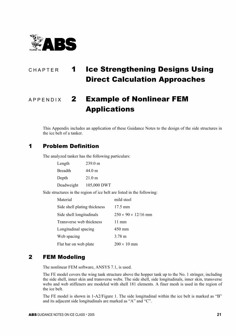
This Appendix includes an application of these Guidance Notes to the design of the side structures in the ice belt of a tanker.
1 Problem Definition The analyzed tanker has the following particulars:
Length 239.0 m
Breadth 44.0 m
Depth 21.0 m
Deadweight 105,000 DWT
Side structures in the region of ice belt are listed in the following:
Material mild steel
Side shell plating thickness 17.5 mm
Side shell longitudinals 250 × 90 × 12/16 mm
Transverse web thickness 11 mm
Longitudinal spacing 450 mm
Web spacing 3.78 m
Flat bar on web plate 200 × 10 mm
2 FEM Modeling The nonlinear FEM software, ANSYS 7.1, is used.
The FE model covers the wing tank structure above the hopper tank up to the No. 1 stringer, including the side shell, inner skin and transverse webs. The side shell, side longitudinals, inner skin, transverse webs and web stiffeners are modeled with shell 181 elements. A finer mesh is used in the region of the ice belt.
The FE model is shown in 1-A2/Figure 1. The side longitudinal within the ice belt is marked as “B” and its adjacent side longitudinals are marked as “A” and “C”.
Chapter 1 Ice Strengthening Using Direct Calculation Approaches Appendix 2 Example of Nonlinear FEM Applications 1-A2
22 ABS GUIDANCE NOTES ON ICE CLASS . 2005
FIGURE 1 FE Model
(a) FE Model
A
B
C
(b) Side shell and side longitudinals (c) Zoom-in of side longitudinals

Chapter 1 Ice Strengthening Using Direct Calculation Approaches Appendix 2 Example of Nonlinear FEM Applications 1-A2
ABS GUIDANCE NOTES ON ICE CLASS . 2005 23
3 Ice Load The maximum ice pressure is calculated as 1.4819 MPa. The corresponding maximum line load on the side longitudinal is 370.5 MN/mm.
1-A2/Figure 2 shows the load paths used in the nonlinear FEM analysis. The load is incrementally increased to the maximum value in the loading phase, and then gradually decreased in the unloading phase. For both loading and unloading phases, 10 load steps are used.
FIGURE 2 Load Path (Loading and Unloading Phases)
0.0
0.2
0.4
0.6
0.8
1.0
1.2
1.4
1.6
Ice
Pres
sure
, MPa
Loading Unloading
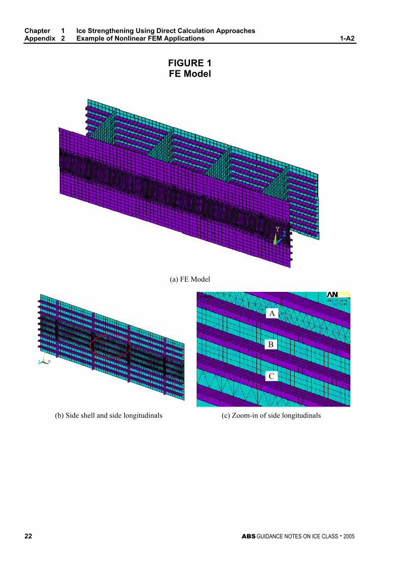
4 Analysis Results 1-A2/Figure 3 shows the stress contours at the end of the loading and unloading phases.
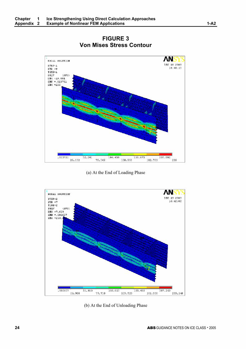
1-A2/Figure 4 shows the load-deflection curves of the three side longitudinals marked with “A”, “B” and “C” in 1-A2/Figure 1. The deflections are in the vessel’s transverse direction.
Chapter 1 Ice Strengthening Using Direct Calculation Approaches Appendix 2 Example of Nonlinear FEM Applications 1-A2
24 ABS GUIDANCE NOTES ON ICE CLASS . 2005
FIGURE 3 Von Mises Stress Contour
(a) At the End of Loading Phase
(b) At the End of Unloading Phase
Chapter 1 Ice Strengthening Using Direct Calculation Approaches Appendix 2 Example of Nonlinear FEM Applications 1-A2
ABS GUIDANCE NOTES ON ICE CLASS . 2005 25
FIGURE 4 Pressure vs. Deflection (Loading and Unloading Phases)
0.0
0.2
0.4
0.6
0.8
1.0
1.2
1.4
1.6
0.0 2.0 4.0 6.0 8.0 10.0 12.0 14.0 16.0 18.0
Deflection, mm
Ice
Pres
sure
, MPa
Long. ALong. BLong. C
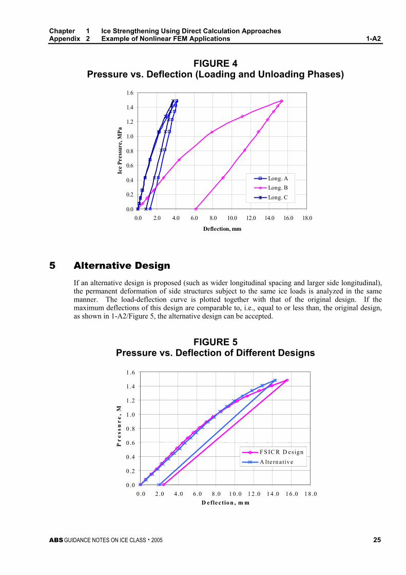
5 Alternative Design If an alternative design is proposed (such as wider longitudinal spacing and larger side longitudinal), the permanent deformation of side structures subject to the same ice loads is analyzed in the same manner. The load-deflection curve is plotted together with that of the original design. If the maximum deflections of this design are comparable to, i.e., equal to or less than, the original design, as shown in 1-A2/Figure 5, the alternative design can be accepted.
FIGURE 5 Pressure vs. Deflection of Different Designs
0 .0 0 .2 0 .4 0 .6 0 .8 1 .0 1 .2 1 .4 1 .6
0 .0 2 .0 4 .0 6 .0 8 .0 1 0 .0 1 2 .0 1 4 .0 1 6 .0 1 8 .0 D eflectio n , m m
Pre
ssu
re,
M
F S IC R D esign A lte rn ativ e

Chapter 1 Ice Strengthening Using Direct Calculation Approaches Appendix 2 Example of Nonlinear FEM Applications 1-A2
26 ABS GUIDANCE NOTES ON ICE CLASS . 2005
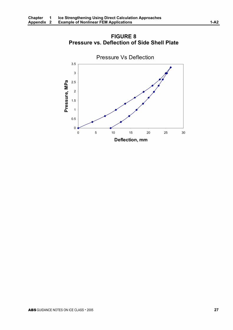
6 Example of Alternative Side Shell Design An example of alternative design of the side shell (1-2/5) is provided below. The FEM modeling process is similar to the previous sample vessel, as required in Chapter 1, Section 2. The sample FEM solutions with deformed side structure under patch ice pressure are shown in 1-A2/Figures 6 and 7, viewed from outside and inside. The patch ice pressure is three times the design ice pressure from the FMA Guidelines. A sample load-deflection curve for the side shell plate during loading and unloading (1-A2/5) is plotted in 1-A2/Figure 8, demonstrating the permanent deformation after unloading.
FIGURE 6 Deformed Side Structure – View from Outside
FIGURE 7 Deformed Side Structure – View from Inside
Chapter 1 Ice Strengthening Using Direct Calculation Approaches Appendix 2 Example of Nonlinear FEM Applications 1-A2
ABS GUIDANCE NOTES ON ICE CLASS . 2005 27
FIGURE 8 Pressure vs. Deflection of Side Shell Plate
Pressure Vs Deflection
0
0.5
1
1.5
2
2.5
3
3.5
0 5 10 15 20 25 30
Deflection, mm
Pres
sure
, MPa

This Page Intentionally Left Blank

ABS GUIDANCE NOTES ON ICE CLASS . 2005 29
Appendix 3: The Finnish Maritime Administration (FMA) “Tentative Note for Application of Direct Calculation Methods for Longitudinally Framed Hull Structure”, 30 June 2003
C H A P T E R 1 Ice Strengthening Designs Using Direct Calculation Approaches
A P P E N D I X 3 The Finnish Maritime Administration (FMA) “Tentative Note for Application of Direct Calculation Methods for Longitudinally Framed Hull Structure”, 30 June 2003
Note: This Appendix is prepared for users’ ready reference to the FMA tentative note. All text contained in the Appendix is taken verbatim from the FMA tentative note.
1 Introduction According to the Finnish-Swedish Ice Class Rules (see FMA Bulletin No. 13/1.10.2002), the maximum frame spacing of longitudinal frames is 0.35 m for ice classes IA Super and IA, and 0.45 m for ice classes IB and IC (see paragraph 4.4.3). In paragraph 4.4.4.1, it is stipulated that longitudinal frames shall be attached to all the supporting web frames and bulkheads by brackets.
In paragraph 4.1, it is said, inter alia, that “For the formulae and values given in this section for the determination of hull scantlings more sophisticated methods may be substituted subject to approval by the administration or the classification society”.
The purpose of these guidelines is to give the modified parameters for the scantling equation for plating, and advise on the calculation of frame section modulus and shear area, if the frame spacing exceeds the stipulated value. Furthermore, advice for a direct calculation procedure is given, if the brackets are omitted.
It should be noted that, in general, the weight of the structure built according to the rules is lower than the weight of a structure with higher longitudinal frame spacing and/or a structure without brackets on the frames. The reason for the application of a higher frame spacing and/or omitting the brackets stems from lower production costs, i.e., a smaller number of structural elements to be welded on the structure.
Chapter 1 Ice Strengthening Using Direct Calculation Approaches Appendix 3 The FMA “Tentative Note for Application of Direct Calculation Methods for
Longitudinally Framed Hull Structure”, 30 June 2003 1-A3
30 ABS GUIDANCE NOTES ON ICE CLASS . 2005
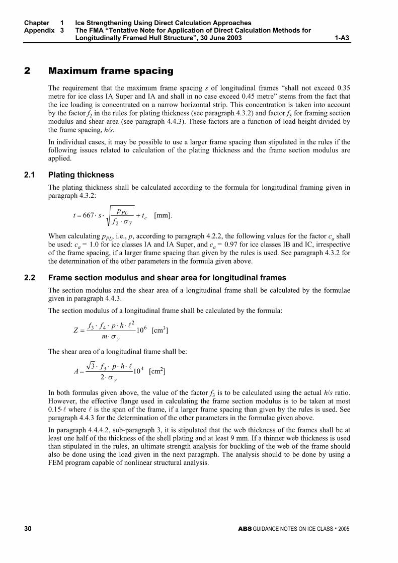
2 Maximum frame spacing
The requirement that the maximum frame spacing s of longitudinal frames “shall not exceed 0.35 metre for ice class IA Super and IA and shall in no case exceed 0.45 metre” stems from the fact that the ice loading is concentrated on a narrow horizontal strip. This concentration is taken into account by the factor f2 in the rules for plating thickness (see paragraph 4.3.2) and factor f3 for framing section modulus and shear area (see paragraph 4.4.3). These factors are a function of load height divided by the frame spacing, h/s.
In individual cases, it may be possible to use a larger frame spacing than stipulated in the rules if the following issues related to calculation of the plating thickness and the frame section modulus are applied.
2.1 Plating thickness The plating thickness shall be calculated according to the formula for longitudinal framing given in paragraph 4.3.2:
cY
PL tf
pst +
⋅⋅⋅=
σ2667 [mm].
When calculating pPL, i.e., p, according to paragraph 4.2.2, the following values for the factor ca shall be used: ca = 1.0 for ice classes IA and IA Super, and ca = 0.97 for ice classes IB and IC, irrespective of the frame spacing, if a larger frame spacing than given by the rules is used. See paragraph 4.3.2 for the determination of the other parameters in the formula given above.
2.2 Frame section modulus and shear area for longitudinal frames The section modulus and the shear area of a longitudinal frame shall be calculated by the formulae given in paragraph 4.4.3.
The section modulus of a longitudinal frame shall be calculated by the formula:
62
43 10ymhpff
Zσ⋅
⋅⋅⋅⋅=
l [cm3]
The shear area of a longitudinal frame shall be:
43 102
3
y
hpfA
σ⋅⋅⋅⋅⋅
=l
[cm2]
In both formulas given above, the value of the factor f3 is to be calculated using the actual h/s ratio. However, the effective flange used in calculating the frame section modulus is to be taken at most 0.15⋅l where l is the span of the frame, if a larger frame spacing than given by the rules is used. See paragraph 4.4.3 for the determination of the other parameters in the formulae given above.
In paragraph 4.4.4.2, sub-paragraph 3, it is stipulated that the web thickness of the frames shall be at least one half of the thickness of the shell plating and at least 9 mm. If a thinner web thickness is used than stipulated in the rules, an ultimate strength analysis for buckling of the web of the frame should also be done using the load given in the next paragraph. The analysis should to be done by using a FEM program capable of nonlinear structural analysis.
Chapter 1 Ice Strengthening Using Direct Calculation Approaches Appendix 3 The FMA “Tentative Note for Application of Direct Calculation Methods for
Longitudinally Framed Hull Structure”, 30 June 2003 1-A3
ABS GUIDANCE NOTES ON ICE CLASS . 2005 31
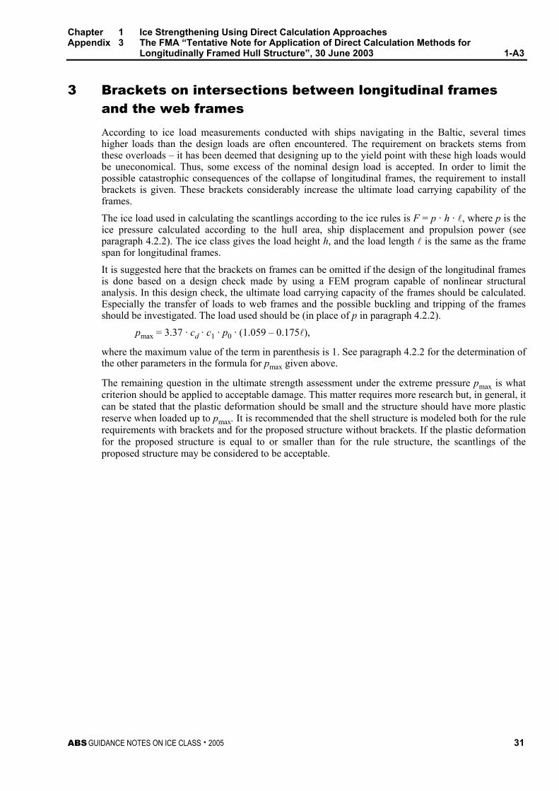
3 Brackets on intersections between longitudinal frames and the web frames According to ice load measurements conducted with ships navigating in the Baltic, several times higher loads than the design loads are often encountered. The requirement on brackets stems from these overloads – it has been deemed that designing up to the yield point with these high loads would be uneconomical. Thus, some excess of the nominal design load is accepted. In order to limit the possible catastrophic consequences of the collapse of longitudinal frames, the requirement to install brackets is given. These brackets considerably increase the ultimate load carrying capability of the frames.
The ice load used in calculating the scantlings according to the ice rules is F = p · h · l, where p is the ice pressure calculated according to the hull area, ship displacement and propulsion power (see paragraph 4.2.2). The ice class gives the load height h, and the load length l is the same as the frame span for longitudinal frames.
It is suggested here that the brackets on frames can be omitted if the design of the longitudinal frames is done based on a design check made by using a FEM program capable of nonlinear structural analysis. In this design check, the ultimate load carrying capacity of the frames should be calculated. Especially the transfer of loads to web frames and the possible buckling and tripping of the frames should be investigated. The load used should be (in place of p in paragraph 4.2.2).
pmax = 3.37 · cd · c1 · p0 · (1.059 – 0.175l),
where the maximum value of the term in parenthesis is 1. See paragraph 4.2.2 for the determination of the other parameters in the formula for pmax given above.
The remaining question in the ultimate strength assessment under the extreme pressure pmax is what criterion should be applied to acceptable damage. This matter requires more research but, in general, it can be stated that the plastic deformation should be small and the structure should have more plastic reserve when loaded up to pmax. It is recommended that the shell structure is modeled both for the rule requirements with brackets and for the proposed structure without brackets. If the plastic deformation for the proposed structure is equal to or smaller than for the rule structure, the scantlings of the proposed structure may be considered to be acceptable.

This Page Intentionally Left Blank
ABS GUIDANCE NOTES ON ICE CLASS . 2005 33
Chapter 2: Power Requirement for Ice Class
C H A P T E R 2 Power Requirement for Ice Class
CONTENTS SECTION 1 Introduction ..........................................................................35 SECTION 2 Alternative Methods to Calculate KC...................................37
1 General ................................................................................37 1.1 Analytical Formula for Required Power in Ice P .............. 37
2 Direct Calculation of KC Value .............................................39 2.1 Model Test Results ......................................................... 39 2.2 Numerical Simulation ...................................................... 40 2.3 Regression Formula........................................................ 40
TABLE 1 KC Value in FSICR .....................................................37
SECTION 3 Alternative Methods to Determine Rch (Resistance in
Brash Ice)..............................................................................41 1 Description of Ice Cover.......................................................41 2 Estimation of Resistance in Broken Channel ......................41 FIGURE 1 Definition Sketch – Brash Ice Channel Geometry .....43
SECTION 4 References............................................................................45 APPENDIX 1 Examples ..............................................................................47
TABLE 1 Wageningen B5-75 Screw Propeller (5 Blades with Area Ratio 0.75).........................................................47
TABLE 2 Ducted Propellers with Nozzle No. 19A, Ka 4-70 Propeller.....................................................................47
TABLE 3 Ducted Propellers with Nozzle No. 37, Ka 4-70 Propeller.....................................................................48
TABLE 4 Ducted Propellers with Nozzle No. 33, Kd 5-100 Propeller.....................................................................48

This Page Intentionally Left Blank

ABS GUIDANCE NOTES ON ICE CLASS . 2005 35
C H A P T E R 2 Power Requirement for Ice Class
S E C T I O N 1 Introduction
6-1-6/9 of the ABS Rules for Building and Classing Steel Vessels stipulates the minimum engine output power which an ice-classed vessel ought to have. The minimum engine power requirement varies depending on the Baltic Ice Classes notations (IAA, IA, IB or IC). These requirements are in line with the Finnish-Swedish Ice Class Rules in its entirety. Therefore, once an ice class notation is granted by ABS based on the ABS Rules, it is considered that the Finnish-Swedish Ice Class Rules have also been complied with for the corresponding ice class designation (IA Super, IA, IB or IC). In the Rules, the minimum required engine output power is calculated in a prescriptive manner by using the following simple formula:
p
chC D
RKP
2/3)1000/( kW ............................................................................................. (1.1)
where
KC = efficiency of propeller(s), obtained from the tables in the Rules once the geometry of the vessel and the propeller(s) are specified
Rch = resistance of the vessel, obtained from the tables in the Rules once the geometry of the vessel and the propeller(s) are specified
Dp = diameter of the propeller(s).
This power requirement is meant to provide vessels with the minimum navigating speed of 5 knots, regardless of the ice class notation, in the ice channel conditions as follows.
Performance Requirement
Class Speed (knots) Channel Thickness (m) Consolidated Layer(m)
IA Super 5 1 0.1
IA 5 1 0
IB 5 0.8 0
IC 5 0.6 0
The Rules, however, allow alternative methods of calculating the minimum required engine power which could demonstrate that the above performance requirements are met, instead of using the simple prescriptive calculation methods in Equation 1.1. It is known that the simplified calculation is conservative in certain instances, and therefore, the alternative calculation methods could yield lower minimum power requirements. The alternative methods involve detailed calculation of KC and Rch based on a more analytical approach. The subsequent Sections explain in detail about the methods which can be adopted in order to work out these two parameters.

This Page Intentionally Left Blank
ABS GUIDANCE NOTES ON ICE CLASS . 2005 37
Section 2: Alternative Methods to Calculate KC
C H A P T E R 2 Power Requirement for Ice Class
S E C T I O N 2 Alternative Methods to Calculate KC
1 General
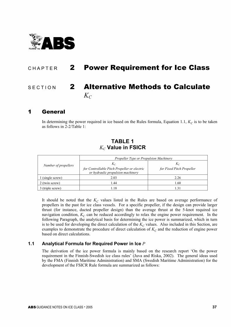
In determining the power required in ice based on the Rules formula, Equation 1.1, KC is to be taken as follows in 2-2/Table 1:
TABLE 1 KC Value in FSICR
Propeller Type or Propulsion Machinery
Number of propellers KC for Controllable Pitch Propeller or electric
or hydraulic propulsion machinery
KC for Fixed Pitch Propeller
1 (single screw) 2.03 2.26 2 (twin screw) 1.44 1.60 3 (triple screw) 1.18 1.31
It should be noted that the KC values listed in the Rules are based on average performance of propellers in the past for ice class vessels. For a specific propeller, if the design can provide larger thrust (for instance, ducted propeller design) than the average thrust at the 5-knot required ice navigation condition, KC can be reduced accordingly to relax the engine power requirement. In the following Paragraph, the analytical basis for determining the ice power is summarized, which in turn is to be used for developing the direct calculation of the KC values. Also included in this Section, are examples to demonstrate the procedure of direct calculation of KC and the reduction of engine power based on direct calculations.
1.1 Analytical Formula for Required Power in Ice P The derivation of the ice power formula is mainly based on the research report ‘On the power requirement in the Finnish-Swedish ice class rules’ (Juva and Riska, 2002). The general ideas used by the FMA (Finnish Maritime Administration) and SMA (Swedish Maritime Administration) for the development of the FSICR Rule formula are summarized as follows:

Chapter 2 Power Requirement for Ice Class Section 2 Alternative Methods to Calculate KC 2-2
38 ABS GUIDANCE NOTES ON ICE CLASS . 2005
1.1.1 Ice Resistance and Thrust Under Ice Operating Condition As is known, for an ice class vessel with a certain moving speed:
Total thrust = Tnet (net thrust to overcome ice resistance Rch) + Open water resistance
Under bollard pull condition, as the vessel speed is zero, the open water resistance becomes zero and the bollard pull thrust is totally used to overcome the ice resistance, i.e.:
Tnet (net thrust to overcome ice resistance Rch) = Tbp (Bollard pull thrust)
1.1.2 Relationship between Bollard Pull Thrust and Thrust Under Ice Operating Condition The net thrust, Tnet, is a function of vessel speed, and it can be approximated by a quadratic factor and the bollard pull thrust (Juva and Riska, 2002) as follows:
bpowow
net TVV
VVT
⎥⎥
⎦
⎤
⎢⎢
⎣
⎡⎟⎟⎠
⎞⎜⎜⎝
⎛−−=
2
32
311
where
Tnet = net thrust used to overcome ice resistance under vessel speed V
Tbp = thrust under bollard pull condition
V = vessel speed under consideration (for ice operating condition V = 5 knots)
Vow = open-water vessel speed
It should be noted that when the vessel speed is zero, the net thrust is equal to bollard pull thrust. When the vessel speed reaches the open-water speed, the net thrust is zero.
In the FSICR, the vessel speed required under ice operating condition is at least 5 knots. Therefore:
Tnet = fTbp ................................................................................................................ (2.1)
where
f = ⎟⎟⎠
⎞⎜⎜⎝
⎛−− 23
503
51owow VV
For open water vessel speed = 15, V/Vow = 5/15 and Tnet = 0.8Tbp.
1.1.3 Bollard Pull Thrust For bollard pull, the relationship between the thrust, Tbp, propeller diameter, Dp, and engine delivered horsepower, P, can easily be derived by eliminating the revolutions per second n and torque, Q, from the definitions of the thrust coefficient, KT, the torque coefficient, KQ, and the engine delivered horsepower, P. Thus by definition:
42p
bpT
Dn
TK
ρ= , 52
pQ
DnQK
ρ= , and P = 2πnQ
then
( ) 3/2323/2 4
PQ
Tbp PD
KK
Tπρ
=
To take the wake effect after the vessel into account, a thrust reduction factor (1 – t) is added back to the above equation:

Chapter 2 Power Requirement for Ice Class Section 2 Alternative Methods to Calculate KC 2-2
ABS GUIDANCE NOTES ON ICE CLASS . 2005 39
( ) )1(4
3/2323/2 tPD
KK
T PQ
Tbp −=
πρ ........................................................................ (2.2)
Usually, t can be taken as 0.02~0.03 (Isin, 1987).
1.1.4 Propulsion Power Formula From Equations 2.1 and 2.2:
( ) )1(4
3/2323/2 tPD
KK
ffTT PQ
Tbpnet −==
πρ
Tnet is the net thrust used to overcome ice resistance which should be equal to Rch:
( ) )1(4
3/2323/2 tPD
KK
fR PQ
Tch −=
πρ
By rearranging the equation:
( )P
ch
T
Q
DR
tfK
KP
2/3
3
1000/
)]1([
2
−=
ρ
π kW
Let 3)]1([
2
tfK
KK
T
QC
−=
ρ
π, and the power formula can be written as the exact form of the
Rules formula (Equation 1.1) as before.
For KC, it can be rearranged as follows:
2/3)(1
eC
fKK = ..................................................................................................... (2.3)
where
)1(4
323/2 t
KK
KQ
Te −=
πρ
Note that KT and KQ are thrust and torque coefficients at the bollard pull condition.
2 Direct Calculation of KC Value
Calculation of the KC value is based on Equation 2.3. As seen in the formula, the KC calculation involves the KT and KQ values at the bollard pull condition, which are dependent on the propeller geometry, its size and rotation speed. Their values can be determined by using model testing, numerical simulation or regression formulae, if the propellers used are standard series propellers.
2.1 Model Test Results Model tests can be used to determine the KT and KQ values. The performance of the model tests can be based on the general practices in different model basins or the 2002 ITTC-recommended procedure (7-5-02-03-02.1). For full-scale extrapolation from the model testing result, the 1978 ITTC-recommended procedure – Performance, Propulsion 1978 ITTC Performance Prediction Method can be adopted (7.5-02-03-01.4, 1999). Usually, the full-scale effect will increase KT and decrease KQ values, thereby further relaxing the engine power requirement.
Chapter 2 Power Requirement for Ice Class Section 2 Alternative Methods to Calculate KC 2-2
40 ABS GUIDANCE NOTES ON ICE CLASS . 2005
2.2 Numerical Simulation Either a potential flow-based model, such as lifting surface code, or a more advanced CFD (Computational Fluid Dynamics) calculation based on RANS (Reynolds Averaged Navier-Stokes) equations can be applied to determine the KT and KQ values. In any case, the simulation programs used should be appropriately validated based on benchmark experimental data. For review of those simulation methods, refer to the 22nd ITTC – the Propulsion committee final report and recommendations (1999).
2.3 Regression Formula If the standard series propeller such as Wageningen B-screen series propeller, Gawn propeller series, Duct nozzle 19A and 37 with Ka propeller, Kd 5-100 nozzle propeller, a regression formula can be used for determining the values of KT and KQ. These regression formulae can be found in the relevant literature (Lammeren et al, 1969 and Principles of Naval Architecture). Similar to model testing approaches, if regression formulae were developed based on model scale testing, the KT and KQ values can be modified based on the 1978 ITTC procedure.

ABS GUIDANCE NOTES ON ICE CLASS . 2005 41
Section 3: Alternative Methods to Determine Rch (Resistance in Brash Ice)
C H A P T E R 2 Power Requirement for Ice Class
S E C T I O N 3 Alternative Methods to Determine Rch (Resistance in Brash Ice)
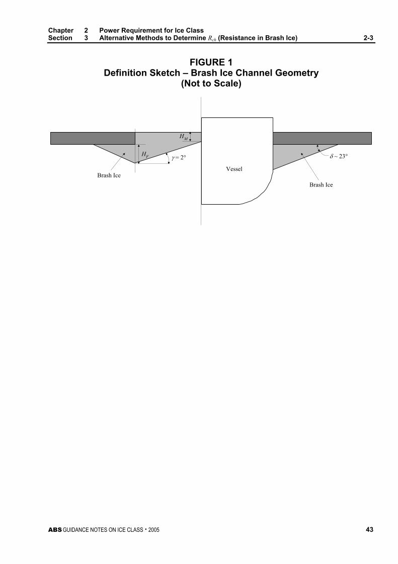
1 Description of Ice Cover Winter navigation channels in the Baltic usually have a thick layer of brash ice cover. Brash ice is formed by a mixture of rounded ice fragments of varying size. The common piece size is around 30 cm, with significant variation depending on the original thickness of the ice cover, vessel traffic frequency in channel, temperature variation, etc. In the worst case, there will also be a thin layer of freshly-frozen level ice on top of the brash ice, the thickness of which is observed to be around 10 cm. These navigation channels are also bounded by side ridges that limit the movements of the brash ice in the channel. 2-3/Figure 1 depicts the parameters of brash ice channel geometry with reference to vessel beam.
It has been observed in practice that ice thickness at the center of the channel is lower than that at the sides, and that the thickness linearly increases from the center toward the sides, the average slope of the thickness variation being 2 degrees. In general, the relationship between the thickness, hi, of the unbroken level ice cover and the thickness, HM, of brash ice at the center of the channel is complex, but observations have shown that HM and hi are roughly of the same magnitude. Further, the brash ice is also pushed under the intact unbroken ice cover at the channel sides, with the average slope of this wedge being 23 degrees. The thickness, HF, represents the brash ice wedge displaced by the bow and moved to the side and pushing against the parallel body. This thickness is a function of the vessel’s beam, the thickness in the channel and the cohesive properties of the brash ice.
2 Estimation of Resistance in Broken Channel As the brash ice piece size is much smaller than a typical length dimension, the assumption of treating the ice mass as a continuum is valid and the brash ice mass can be modeled as a Mohr-Coulomb material. Without going into the details of derivation, the basis of the brash ice resistance formulation can be summarized. The resistance to motion in brash ice is assumed to be due only to the forces required to submerge the ice as well as to displace it sideways. Simplifications are made in the method for quantifying both of the above components.
The total force arising from the above can be formulated to have a resultant component normal to the hull at the bow, which will also yield the hull-ice friction force that can be resolved into the required directions. Although the thin consolidated layer does not necessarily have the same properties as level ice, and despite the fact that this thin layer is not supported by water, but by the brash ice layer, for computational purposes, it is treated as level ice and its breaking resistance is superimposed on the brash ice resistance.

Chapter 2 Power Requirement for Ice Class Section 3 Alternative Methods to Determine Rch (Resistance in Brash Ice) 2-3
42 ABS GUIDANCE NOTES ON ICE CLASS . 2005
Resolution of ice forces normal to the hull into their components along the longitudinal (fore-and-aft) direction would involve the hull angles. For level ice breaking, these are measured at the bow on centerline, where most of the icebreaking forces are generated. However, this is not true for bow interaction with brash ice, wherein the entire bow is displacing the ice, thereby developing the hull resistance. Thus, an average value of the hull angles over the length of the bow would be the most suitable, in which case, the bow is approximated as a wedge having straight sides. The hull resistance in a brash ice channel can then be expressed as follows:
( )
23
22
22 sinsincos
tan1cos2
221
21
FnAHBLTgHLgK
HBH
HKgHR
WFMFparHoB
HFF
MPFBch
⎥⎦
⎤⎢⎣
⎡Δ+Δ+
+⎥⎦
⎤⎢⎣
⎡⎟⎟⎠
⎞⎜⎜⎝
⎛−+⎥
⎦
⎤⎢⎣
⎡+Δ=
ρμρμ
αψφμψ
δρμ
δγ
γδγγ
tantan
tan4)tan(tantan
2 +
⎥⎦⎤
⎢⎣⎡ +
+++=
BHBBHH
M
MF
where
L = length, m
Lpar = length of parallel midbody at waterline, m
Lbow = length of the foreship at waterline, m
AWF = waterplane area of foreship, m2
B = breadth, m
T = draft, m
φ = angle between the waterline and vertical at B/2, deg
ψ = flare angle, deg
α = waterplane entrance angle, deg
hi = level ice thickness, m
HM = brash ice thickness in the middle of the channel, m
HF = thickness of brash ice against the parallel midbody, m
μB = 1 – porosity = 0.8 to 0.9
μH = hull-ice friction coefficient
Δρ = difference in densities
δ = slope angle of brash ice at 23.0 deg
g = acceleration due to gravity
v = vessel speed, m/s (kn)
ρ = water density, ton/m3
Chapter 2 Power Requirement for Ice Class Section 3 Alternative Methods to Determine Rch (Resistance in Brash Ice) 2-3
ABS GUIDANCE NOTES ON ICE CLASS . 2005 43
FIGURE 1 Definition Sketch – Brash Ice Channel Geometry
(Not to Scale)
HF
HM
γ = 2° δ ~ 23°
Vessel
Brash IceBrash Ice

This Page Intentionally Left Blank
ABS GUIDANCE NOTES ON ICE CLASS . 2005 45
Section 4: References
C H A P T E R 2 Power Requirement for Ice Class
S E C T I O N 4 References
Isin, Y.A., 1987 ‘Practical bollard-pull estimation’, Marine Technology, Vol. 24, No. 3, July 1987, pp 220-225
ITTC recommended procedures – Testing and extrapolation methods propulsion, Propulsor Open Water Test 7.5-02-03-2.1 (effective date 2002)
ITTC recommended procedures – Performance, Propulsion 1978 ITTC Performance Prediction Method 7.5-02-03-01.4 (effective date 1999)
ITTC the propulsion committee – final report and recommendation (1999)
Juva, M. and Riska, K., 2002, ‘On the Power Requirement in the Finish-Swedish Ice Class Rules’, Research report no. 53, Helsinki University of Technology, Ship Laboratory.
Lammeren, W.P.A. van, Manen, J.D. van, Oosterveld, M.W.C., ‘The Wageningen B-screw series’, Trans. SNAME, 1969.
Riska, K., et al, Performance of Merchant Vessels in the Baltic, Research Report No. 52, Winter Navigation Research Board, 1997.
SNAME ‘Principles of Naval Architecture’, vol. 2, pp 222-225.

This Page Intentionally Left Blank
ABS GUIDANCE NOTES ON ICE CLASS . 2005 47
Appendix 1: Examples
C H A P T E R 2 Power Requirement for Ice Class
A P P E N D I X 1 Examples
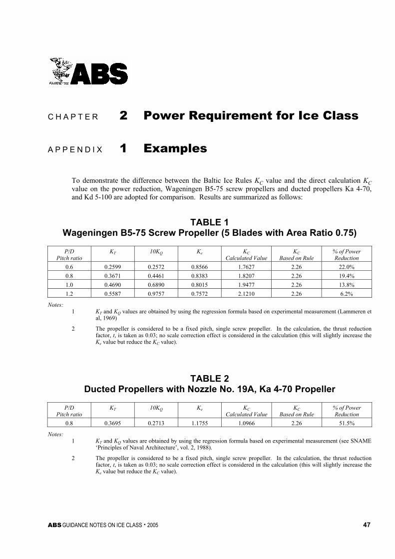
To demonstrate the difference between the Baltic Ice Rules KC value and the direct calculation KC value on the power reduction, Wageningen B5-75 screw propellers and ducted propellers Ka 4-70, and Kd 5-100 are adopted for comparison. Results are summarized as follows:
TABLE 1 Wageningen B5-75 Screw Propeller (5 Blades with Area Ratio 0.75)
P/D Pitch ratio
KT 10KQ
Ke KC Calculated Value
KC Based on Rule
% of Power Reduction
0.6 0.2599 0.2572 0.8566 1.7627 2.26 22.0% 0.8 0.3671 0.4461 0.8383 1.8207 2.26 19.4% 1.0 0.4690 0.6890 0.8015 1.9477 2.26 13.8% 1.2 0.5587 0.9757 0.7572 2.1210 2.26 6.2%
Notes: 1 KT and KQ values are obtained by using the regression formula based on experimental measurement (Lammeren et
al, 1969)
2 The propeller is considered to be a fixed pitch, single screw propeller. In the calculation, the thrust reduction factor, t, is taken as 0.03; no scale correction effect is considered in the calculation (this will slightly increase the Ke value but reduce the KC value).
TABLE 2 Ducted Propellers with Nozzle No. 19A, Ka 4-70 Propeller
P/D Pitch ratio
KT 10KQ
Ke KC Calculated Value
KC Based on Rule
% of Power Reduction
0.8 0.3695 0.2713 1.1755 1.0966 2.26 51.5%
Notes: 1 KT and KQ values are obtained by using the regression formula based on experimental measurement (see SNAME
‘Principles of Naval Architecture’, vol. 2, 1988).
2 The propeller is considered to be a fixed pitch, single screw propeller. In the calculation, the thrust reduction factor, t, is taken as 0.03; no scale correction effect is considered in the calculation (this will slightly increase the Ke value but reduce the KC value).
Chapter 2 Power Requirement for Ice Class Appendix 1 Examples 2-A1
48 ABS GUIDANCE NOTES ON ICE CLASS . 2005
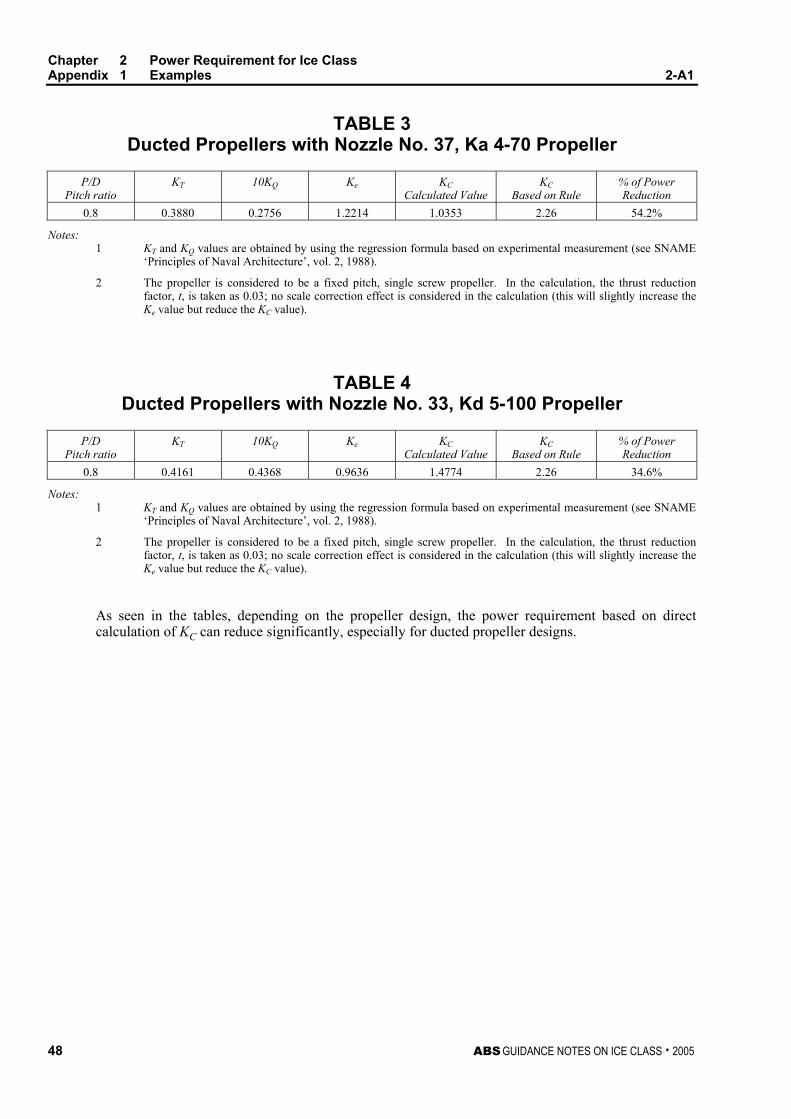
TABLE 3 Ducted Propellers with Nozzle No. 37, Ka 4-70 Propeller
P/D Pitch ratio
KT 10KQ
Ke KC Calculated Value
KC Based on Rule
% of Power Reduction
0.8 0.3880 0.2756 1.2214 1.0353 2.26 54.2%
Notes: 1 KT and KQ values are obtained by using the regression formula based on experimental measurement (see SNAME
‘Principles of Naval Architecture’, vol. 2, 1988).
2 The propeller is considered to be a fixed pitch, single screw propeller. In the calculation, the thrust reduction factor, t, is taken as 0.03; no scale correction effect is considered in the calculation (this will slightly increase the Ke value but reduce the KC value).
TABLE 4 Ducted Propellers with Nozzle No. 33, Kd 5-100 Propeller
P/D Pitch ratio
KT 10KQ
Ke KC Calculated Value
KC Based on Rule
% of Power Reduction
0.8 0.4161 0.4368 0.9636 1.4774 2.26 34.6%
Notes: 1 KT and KQ values are obtained by using the regression formula based on experimental measurement (see SNAME
‘Principles of Naval Architecture’, vol. 2, 1988).
2 The propeller is considered to be a fixed pitch, single screw propeller. In the calculation, the thrust reduction factor, t, is taken as 0.03; no scale correction effect is considered in the calculation (this will slightly increase the Ke value but reduce the KC value).
As seen in the tables, depending on the propeller design, the power requirement based on direct calculation of KC can reduce significantly, especially for ducted propeller designs.
ABS GUIDANCE NOTES ON ICE CLASS . 2005 49
Chapter 3: Propeller Strength Assessment
C H A P T E R 3 Propeller Strength Assessment
CONTENTS SECTION 1 General Design Basis ..........................................................51
1 Scope...................................................................................51 2 Updated Finnish Swedish Ice Class Rules..........................51 3 Ice Load Scenarios Considered In Load Formula
Development........................................................................52 4 Material for Ice Propeller......................................................52 5 Propeller Blade Design ........................................................52
SECTION 2 Ice Load Determination .......................................................53
1 Operation and Environmental Ice Conditions ......................53 2 Design Loads .......................................................................53
2.1 Maximum Forward and Backward Loads ........................ 54 2.2 Ice Load Distributions for Blade Fatigue ......................... 56 2.3 Blade Plastic Failure Load .............................................. 59
TABLE 1 Operations in Different Ice Class ...............................53 TABLE 2 Thickness of Design Maximum Ice Block Hice ............53 TABLE 3 Maximum Loads for Open Propeller ..........................54 TABLE 4 Maximum Loads for Ducted Propeller .......................54 TABLE 5 Load Cases for Open Propeller .................................55 TABLE 6 Load Cases for Ducted Propeller...............................56 TABLE 7 Nclass for Different Ice Classes ....................................58 TABLE 8 Propeller Location Factor k1 .......................................58 TABLE 9 Propeller Type Factor k2.............................................58 TABLE 10 Propulsion Type Factor k3 ..........................................58 FIGURE 1 Weibull-type Distributions with Shape Parameters
k = 0.75 and 1.0 .........................................................57 FIGURE 2 Physical Meaning of f.................................................59
SECTION 3 Blade Stress Analysis Procedure.......................................61
1 Simple Formula for Conventional Propeller .........................61 2 FEM Direct Calculation for Highly Skewed Propeller ..........61
2.1 Fatigue ............................................................................62 2.2 Plastic Failure..................................................................65

50 ABS GUIDANCE NOTES ON ICE CLASS . 2005
TABLE 1 Values of Coefficients C1, C2, C3 and C4.....................63 TABLE 2 Values for the Gamma Function, Γ(m/k + 1)...............64 FIGURE 1 Two-slope S-N Curve.................................................63 FIGURE 2 Single-slope S-N Curve .............................................64
SECTION 4 Summary of Propeller Strength Assessment
Procedure ............................................................................. 67 FIGURE 1 Flowchart of Assessment Procedure of Propeller
Strength......................................................................67 SECTION 5 References............................................................................ 69 APPENDIX 1 Illustrative Example ............................................................. 71
1 Information Required for Blade Strength Check..................71 2 Load Determination..............................................................73
2.1 Stress Analysis................................................................73 3 Blade Strength Check ..........................................................77 TABLE 1 Calculated Maximum Stresses (von Mises) for
40 × 30 & 80 × 60 Meshes .........................................73 TABLE 2 Differences Between the Results of 40 × 30 and
80 × 60 Meshes..........................................................73 TABLE 3 Calculation of (σice)max .................................................77 FIGURE 1 Blade Section Offsets ................................................72 FIGURE 2 Propeller Geometry Plot.............................................72 FIGURE 3 Meshes and Blade Pressure used in Illustrative
Example .....................................................................74 FIGURE 4 Stress (von Mises) Distribution on Back Side
(40 × 30 Meshes) .......................................................75 FIGURE 5 Stress (von Mises) Distribution on Face Side
(40 × 30 Meshes) .......................................................76 FIGURE 6 Principal Stress Distribution on Back Side
(80 × 60 Meshes) .......................................................78 FIGURE 7 Principal Stress Distribution on Face Side
(80 × 60 Meshes) .......................................................79

ABS GUIDANCE NOTES ON ICE CLASS . 2005 51
Section 1: General Design Basis
C H A P T E R 3 Propeller Strength Assessment
S E C T I O N 1 General Design Basis
1 Scope In propeller strength assessment, the updated Finnish-Swedish Ice Class Rules (Draft Proposal for the Finnish Swedish Ice Class Rules for Propulsion Machinery, Rev. 2, 2004) requests that all IAA class propellers and highly skewed propellers in IA, IB, and IC classes be subjected to detailed FEM-based stress analysis. Instead of simple formulae based on beam theory, which are usually provided in Classification Societies’ Rules, FEM analysis requests more technical details, such as an FE model, the load application to the FE model and the stress results interpretation. The purpose of this Chapter is to provide a clearly-defined propeller strength assessment procedure for ice class vessels based on the latest Finnish-Swedish Ice Class Rules. Also, through an illustrative example, more technical details regarding the performance of fatigue and plastic failure analysis in the blade strength assessment procedure are provided.
2 Updated Finnish Swedish Ice Class Rules The Finnish-Swedish Ice Class Rules (1971) for propulsion machinery was based on the use of ice torque as the dimensioning load [1]. The blade ice load is then obtained on the basis of the ice torque. However, recent experimental and theoretical research on propeller blade loads indicated that the ice torque principle did not accurately reflect the physical phenomena causing the ice loads on the propeller. Although the ice torque principle could provide sufficient scantlings for a conventional propeller, its application to highly skewed propellers was deemed questionable.
Background work for renewal of the 1971 FSICR Rules was initiated by the Board of Navigation, and a preliminary proposal for new ice class rules was worked out at the end of the 1980’s. At that time, it was concluded that there was not enough knowledge of the propeller ice loads for renewing the ice class rules. The Canadian Coast Guard and Finnish Board of Navigation established a joint research project ‘JRPA#6, Propeller/Ice Interaction’ in 1991, aimed at the development of a new propeller/ice interaction model. The ultimate goal was to use the model in formulating new machinery regulations for the Arctic and the Baltic ice conditions. The JRPA#6 project was completed at the end of 1995. The new ice class rule proposal has been developed based on the understanding of the propeller/ice interaction phenomena and the load formulations on the research work that was conducted during the JRPA#6 project [2].

Chapter 3 Propeller Strength Assessment Section 1 General Design Basis 3-1
52 ABS GUIDANCE NOTES ON ICE CLASS . 2005
3 Ice Load Scenarios Considered In Load Formula Development There are two types of interactions between ice and propellers, namely ice milling and ice impact. Ice milling takes place when an ice block is large or is trapped between the hull and the propeller. During an instance of milling, ice is either crushed or sheared by the blades, and the loads can be damagingly high. Ice impact is caused by small-size ice pieces that are accelerated through a propeller or thrown out radially and pushed around the edge of the propeller disk. The loads from ice impact are relatively moderate, but occur more frequently.
For a propeller in a nozzle, the chances of ice milling are small, and the magnitude of the loads generated is also small in comparison to those for open propellers. The factors that influence the ice loading on a propeller have been studied in the joint research project “JRPA #6, Propeller/Ice Interaction,” and load formulae have been developed through numerical studies.
4 Material for Ice Propeller The material used for the propeller blades of ice class vessels must have high stress and impact resistance qualities. Stainless steel and bronze are commonly used for ice-strengthened propeller blades. Because stainless steel has a higher erosion resistance and higher ultimate and yielding strengths than bronze, stainless steel propellers can have a more slender and efficient blade profile than bronze propellers. Most of the existing bronze controllable-pitch propellers fitted to ice class vessels are open propellers.
According to the updated Finnish Swedish Ice Class Rule (FSICR), “materials exposed to sea water, such as propeller blades, propeller hub and blade bolts shall have an elongation not less than 15% on a test piece the length of which is five times the diameter. Charpy impact test shall be carried out for other than bronze materials. Test pieces taken from the propeller blade shall be representative of the thickest section of the blade, in the weakest direction. An average impact energy value of 20 J taken from three tests is to be obtained at minus 10°C, and is not to be less than 0.8 of the value at 20°C.”
5 Propeller Blade Design A comprehensive design study is to be carried out to meet the dimensions and the strength requirements of the classification society. The study is to be based on ice loading conditions given for different ice classes in the updated FSICR. Both fatigue and maximum load design calculations are to be performed. In addition, the pyramid strength principle, which requires that the loss of the propeller blade shall not cause any significant damages in other propeller shaft line components, is to be fulfilled.

ABS GUIDANCE NOTES ON ICE CLASS . 2005 53
Section 2: Ice Load Determination
C H A P T E R 3 Propeller Strength Assessment
S E C T I O N 2 Ice Load Determination
1 Operation and Environmental Ice Conditions
Environmental ice conditions at the operational area provide the basis for class restrictions. Links have to be made between the ice conditions and propeller loading. This requires a design ice thickness related to the class definition of nominal ice condition. According to the updated FSICR, the ice loads of the propeller for ice classes are estimated taking into account the different types of operations, as summarized in 3-2/Table 1. For estimation of design ice loads, a maximum ice block size is determined. The maximum design ice block entering the propeller is a rectangular ice block having dimensions Hice × 2Hice × 3Hice. The thickness of the ice block Hice is listed in 3-2/Table 2.
TABLE 1 Operations in Different Ice Class
Ice Class IAA IA IB IC Operation of the vessel Operation in ice channels and in level ice.
The vessel may proceed by ramming. Operation in ice channels.
TABLE 2 Thickness of Design Maximum Ice Block Hice
Ice Class IAA IA IB IC Thickness of the design maximum ice block entering the propeller (Hice)
1.75 m 1.5 m 1.2 m 1.0 m
2 Design Loads According to the updated FSICR, the loads in ice class propellers are expected to be ice loads during the whole vessel’s service life for normal operational conditions, including loads due to rotational direction changing if a fixed pitch propeller is under consideration. The formulae summarized below are the maximum lifetime force on a propeller blade due to propeller ice interaction, including hydrodynamic loads on that blade. The direction of the force is perpendicular to the 0.7 propeller radius chord line.
If the propeller is not fully submerged when the vessel is in ballast condition, the propulsion system shall be designed according to ice class IA for ice classes IB and IC.

Chapter 3 Propeller Strength Assessment Section 2 Ice Load Determination 3-2
54 ABS GUIDANCE NOTES ON ICE CLASS . 2005
2.1 Maximum Forward and Backward Loads Maximum loads of an ice propeller considered in FSICR are the maximum forces bending a propeller blade backwards and forwards when the propeller mills an ice block while rotating ahead. These forces are originating from different propeller/ice interaction phenomena, not acting simultaneously. They are to be applied on one blade separately. Ice load formulae are summarized as follows for open and ducted propeller (3-2/Tables 3 and 4).
TABLE 3
Maximum Loads for Open Propeller
Max. backward blade force Fb Max. forward blade force Ff
For D ≤ Dlimit
23.0
7.0][4.33 DZ
EARnDFb ⎥⎦⎤
⎢⎣⎡= kN....................(2.1a)
For D > Dlimit
4.13.0
7.0][2.29 iceb DHZ
EARnDF ⎥⎦⎤
⎢⎣⎡= kN............. (2.1b)
where Dlimit = 0.87 4.1iceH m
For D ≤ Dlimit
2314 DZ
EARFb ⎥⎦⎤
⎢⎣⎡= kN ..................................(2.2a)
For D > Dlimit
iceb HDd
DZ
EARF/1
1628−⎥⎦
⎤⎢⎣⎡= kN............ (2.2b)
where Dlimit = iceHDd /1
2−
m
D = propeller diameter, in meters EAR = propeller expanded area ratio Z = blade number n = nominal rpm (at MCR condition) for CPP and 85% of rpm (MCR condition) for FPP Hice = thickness of the design maximum ice block in 3-2/Table 2
TABLE 4 Maximum Loads for Ducted Propeller
Max. backward blade force Fb Max. forward blade force Ff
For D ≤ Dlimit
23.0
7.0][5.9 DZ
EARnDFb ⎥⎦⎤
⎢⎣⎡= kN.....................(2.3a)
For D > Dlimit
4.16.03.0
7.0][5.66 iceb HDZ
EARnDF ⎥⎦⎤
⎢⎣⎡= kN ........ (2.3b)
where Dlimit = 0.87 4.1iceH m
For D ≤ Dlimit
2283 DZ
EARFb ⎥⎦⎤
⎢⎣⎡= kN..................................(2.4a)
For D > Dlimit
iceb HDd
DZ
EARF/1
1566−⎥⎦
⎤⎢⎣⎡= kN ............. (2.4b)
where Dlimit = iceHDd /1
2−
m
D = propeller diameter, in meters EAR = propeller expanded area ratio Z = blade number n = nominal rpm (at MCR condition) for CPP and 85% of rpm (MCR condition) for FPP Hice = thickness of the design maximum ice block in 3-2/Table 2

Chapter 3 Propeller Strength Assessment Section 2 Ice Load Determination 3-2
ABS GUIDANCE NOTES ON ICE CLASS . 2005 55
To apply these forces to a blade, FSICR requires that the following cases be considered (3-2/Table 5). For an open propeller, cases 1–4 are to be covered. In order to obtain blade ice loads for reversing rotation of open fixed pitch propeller (FPP), load case 5 is to be considered.
TABLE 5 Load Cases for Open Propeller
Force Loaded Area Case 1 Fb Uniform pressure applied on the
back of the blade (suction side) to an area from 0.6R to the tip and from the leading edge to 0.1 times the chord length
Case 2 0.5Fb Uniform pressure applied on the
back of the blade (suction side) on the propeller tip area outside of 0.9 radius
Case 3 Ff Uniform pressure applied on the
face of the blade (pressure side) to an area from 0.6R to the tip and from the leading edge to 0.1 times the chord length
Case 4 0.5Ff Uniform pressure applied on the
face of the blade (pressure side) on the propeller tip area outside of 0.9 radius
Case 5 0.8 max{Fb, Ff} Uniform pressure applied on
propeller face (pressure side) to an area from 0.6R to the tip and from the trailing edge to 0.1 times the chord length

Chapter 3 Propeller Strength Assessment Section 2 Ice Load Determination 3-2
56 ABS GUIDANCE NOTES ON ICE CLASS . 2005
For a ducted propeller, as the chances of tip contact loads are small, only cases 1 and 3 are required to be considered. Similar to open FPP, load case 5 is needed for ducted FPP (3-2/Table 6).
TABLE 6 Load Cases for Ducted Propeller
Force Loaded Area Case 1 Fb Uniform pressure applied on the
back of the blade (suction side) to an area from 0.6R to the tip and from the leading edge to 0.1 times the chord length
Case 3 Ff Uniform pressure applied on the
face of the blade (pressure side) to an area from 0.6R to the tip and from the leading edge to 0.1 times the chord length
Case 5 0.8 max{Fb, Ff} Uniform pressure applied on
propeller face (pressure side) to an area from 0.6R to the tip and from the trailing edge to 0.1 times the chord length
2.2 Ice Load Distributions for Blade Fatigue As ice loads on a blade occur in a random manner, instead of a deterministic approach usually adopted in non-ice propeller load analysis, a probability method is used in FSICR to determine the fatigue load. In order to express the probability for a random ice load, Fice, to be equivalent to or higher than a given load, F, when exposed to a number of ice load cycles during its lifetime, Nice, a Weibull-type distribution (probability of exceedance) is used for fatigue design of the blade (see Equation 2.5 below). The Weibull-type distribution is illustrated by examples in 3-2/Figure 1, in which probability distributions are plotted for two different shape parameters (k = 0.75 and 1.0) of ice force.
( ) ( )( ) ( )
⎥⎥⎥
⎦
⎤
⎢⎢⎢
⎣
⎡⋅⎟
⎟⎠
⎞⎜⎜⎝
⎛−
=⎥⎥⎦
⎤
⎢⎢⎣
⎡≥
iceNk
iceFF
iceice
ice eF
FF
FP
lnmax
maxmax............................................................ (2.5)
where
k = shape parameter of the spectrum
Nice = number of load cycles in the spectrum
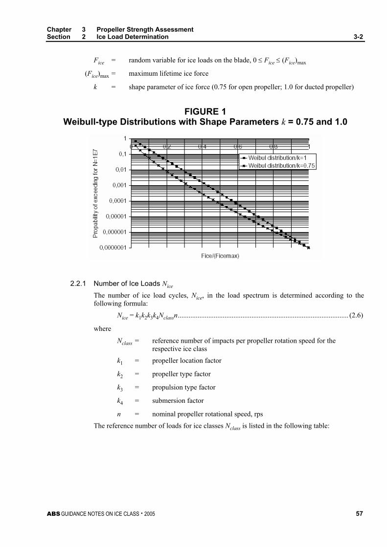
Chapter 3 Propeller Strength Assessment Section 2 Ice Load Determination 3-2
ABS GUIDANCE NOTES ON ICE CLASS . 2005 57
Fice = random variable for ice loads on the blade, 0 ≤ Fice ≤ (Fice)max
(Fice)max = maximum lifetime ice force
k = shape parameter of ice force (0.75 for open propeller; 1.0 for ducted propeller)
FIGURE 1 Weibull-type Distributions with Shape Parameters k = 0.75 and 1.0
2.2.1 Number of Ice Loads Nice The number of ice load cycles, Nice, in the load spectrum is determined according to the following formula:
Nice = k1k2k3k4Nclassn............................................................................................... (2.6)
where
Nclass = reference number of impacts per propeller rotation speed for the respective ice class
k1 = propeller location factor
k2 = propeller type factor
k3 = propulsion type factor
k4 = submersion factor
n = nominal propeller rotational speed, rps
The reference number of loads for ice classes Nclass is listed in the following table:
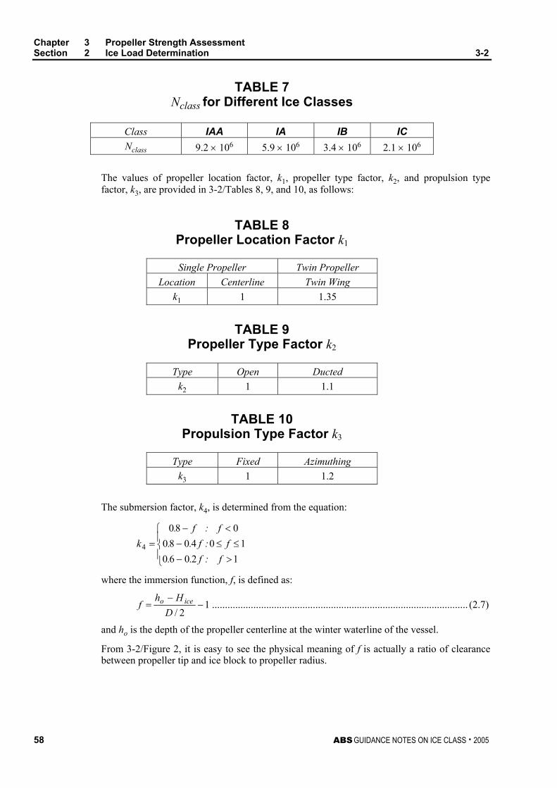
Chapter 3 Propeller Strength Assessment Section 2 Ice Load Determination 3-2
58 ABS GUIDANCE NOTES ON ICE CLASS . 2005
TABLE 7 Nclass for Different Ice Classes
Class IAA IA IB IC Nclass 9.2 × 10⁶ 5.9 × 10⁶ 3.4 × 10⁶ 2.1 × 10⁶
The values of propeller location factor, k1, propeller type factor, k2, and propulsion type factor, k3, are provided in 3-2/Tables 8, 9, and 10, as follows:
TABLE 8 Propeller Location Factor k1
Single Propeller Twin Propeller Location Centerline Twin Wing
k1 1 1.35
TABLE 9 Propeller Type Factor k2
Type Open Ducted k2 1 1.1
TABLE 10 Propulsion Type Factor k3
Type Fixed Azimuthing k3 1 1.2
The submersion factor, k4, is determined from the equation:
110
0
20604080
80
4
>≤≤
<
⎪⎩
⎪⎨
⎧
−−−
=f
ff
:::
f..f..
f.k
where the immersion function, f, is defined as:
12/
−−
=D
Hhf iceo ................................................................................................... (2.7)
and ho is the depth of the propeller centerline at the winter waterline of the vessel.
From 3-2/Figure 2, it is easy to see the physical meaning of f is actually a ratio of clearance between propeller tip and ice block to propeller radius.
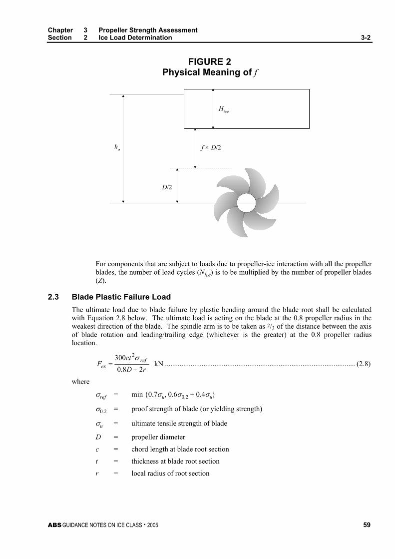
Chapter 3 Propeller Strength Assessment Section 2 Ice Load Determination 3-2
ABS GUIDANCE NOTES ON ICE CLASS . 2005 59
FIGURE 2 Physical Meaning of f
Hice
f × D/2
D/2
ho
For components that are subject to loads due to propeller-ice interaction with all the propeller blades, the number of load cycles (Nice) is to be multiplied by the number of propeller blades (Z).
2.3 Blade Plastic Failure Load The ultimate load due to blade failure by plastic bending around the blade root shall be calculated with Equation 2.8 below. The ultimate load is acting on the blade at the 0.8 propeller radius in the weakest direction of the blade. The spindle arm is to be taken as 2/3 of the distance between the axis of blade rotation and leading/trailing edge (whichever is the greater) at the 0.8 propeller radius location.
rDct
F refex 28.0
300 2
−=
σ kN ........................................................................................................ (2.8)
where
σref = min {0.7σu, 0.6σ0.2 + 0.4σu}
σ0.2 = proof strength of blade (or yielding strength)
σu = ultimate tensile strength of blade
D = propeller diameter
c = chord length at blade root section
t = thickness at blade root section
r = local radius of root section

This Page Intentionally Left Blank
ABS GUIDANCE NOTES ON ICE CLASS . 2005 61
Section 3: Blade Stress Analysis Procedure
C H A P T E R 3 Propeller Strength Assessment
S E C T I O N 3 Blade Stress Analysis Procedure
1 Simple Formula for Conventional Propeller For propellers with conventional design (skew angle < 25°) in ice classes IA, IB, and IC, a simplified formula is available for the blade stress estimation.
21100ctM
C BLst =σ .................................................................................................................. (3.1)
where
C1 = actual stress/stress obtained with beam equation. If the actual value is not available, C1 should be taken as 1.6
c = chord length at local radius r section
t = thickness at local radius r section
MBL = (0.75 – r/R) × F × R for r/R < 0.6
= (0.90 – r/R) × 0.5F × R for 0.6 < r/R < 0.8
F = max{Fb, Ff}
Fb, Ff = maximum forward and backward forces (3-2/2.1)
R = propeller tip radius
2 FEM Direct Calculation for Highly Skewed Propeller If the propeller is a highly skewed design or the propeller is subjected to IAA ice class, the blade stresses should be calculated based on FEM analysis for the design loads given in 3-2/2.1 for final approval.
The requirement for the FE model is that it is able to represent the complex curvilinear geometry and the thickness variation of the blade and also the geometry of the fillet at the root of the blade, in order to represent the complex three-dimensional stress state of the structure and to represent the local peak stresses needed to assess the fatigue strength of the structure within acceptable accuracy. The load on the propeller blade is dominated by bending, leading to non-constant stress distribution over the thickness of the blade. The model should also be able to represent the stress distribution over the thickness of the blade.
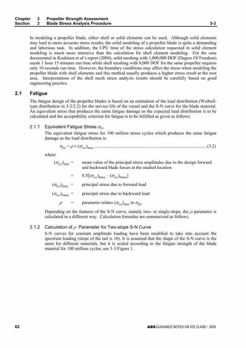
Chapter 3 Propeller Strength Assessment Section 3 Blade Stress Analysis Procedure 3-3
62 ABS GUIDANCE NOTES ON ICE CLASS . 2005
In modeling a propeller blade, either shell or solid elements can be used. Although solid elements may lead to more accurate stress results, the solid modeling of a propeller blade is quite a demanding and laborious task. In addition, the CPU time of the stress calculation requested in solid element modeling is much more intensive than the calculation for shell element modeling. For the case documented in Koskinen et al’s report (2004), solid meshing with 1,000,000 DOF (Degree Of Freedom) needs 1 hour 15 minutes run time while shell meshing with 8,000 DOF for the same propeller requires only 10 seconds run time. However, the boundary conditions may affect the stress when modeling the propeller blade with shell elements and this method usually produces a higher stress result at the root area. Interpretations of the shell mesh stress analysis results should be carefully based on good engineering practice.
2.1 Fatigue The fatigue design of the propeller blades is based on an estimation of the load distribution (Weibull-type distribution in 3-2/2.2) for the service life of the vessel and the S-N curve for the blade material. An equivalent stress that produces the same fatigue damage as the expected load distribution is to be calculated and the acceptability criterion for fatigue is to be fulfilled as given as follows.
2.1.1 Equivalent Fatigue Stress σfat
The equivalent fatigue stress for 100 million stress cycles which produces the same fatigue damage as the load distribution is:
σfat = ρ × (σice)max................................................................................................... (3.2)
where
(σice)max = mean value of the principal stress amplitudes due to the design forward and backward blade forces at the studied location
= 0.5[(σice)fmax – (σice)bmax]
(σice)fmax = principal stress due to forward load
(σice)bmax = principal stress due to backward load
ρ = parameter relates (σice)max to σfat
Depending on the features of the S-N curve, namely two- or single-slope, the ρ parameter is calculated in a different way. Calculation formulae are summarized as follows.
2.1.2 Calculation of ρ Parameter for Two-slope S-N Curve S-N curves for constant amplitude loading have been modified to take into account the spectrum loading (slope of the tail is 10). It is assumed that the shape of the S-N curve is the same for different materials, but it is scaled according to the fatigue strength of the blade material for 100 million cycles, see 3-3/Figure 1.

Chapter 3 Propeller Strength Assessment Section 3 Blade Stress Analysis Procedure 3-3
ABS GUIDANCE NOTES ON ICE CLASS . 2005 63
FIGURE 1 Two Slope S-N Curve
The parameter ρ is relating the maximum ice load to the distribution of ice loads according to the formula:
ρ = ( )[ ] ( ) ( ) 432max1 lg C
iceC
flC
ice NC ⋅⋅⋅ σσ ........................................................... (3.3)
where
σfl = γε ⋅ γν ⋅ γm ⋅ σexp.....................................................................................(3.4)
γε = reduction factor for scatter and test specimen size effect
γν = reduction factor for variable amplitude loading
γm = reduction factor for mean stress
σexp = mean fatigue strength of the blade material at 108 cycles to failure in seawater.
The following values should be used for the reduction factors if actual values are not available: γε = 0.67, γν = 0.75, and γm = 0.75. Coefficients, C1, C2, C3 and C4 are given in the following table:
TABLE 1 Values of Coefficients C1, C2, C3 and C4
Open Propeller Ducted Propeller C1 0.000711 0.000509 C2 0.0645 0.0533 C3 -0.0565 -0.0459 C4 2.22 2.584
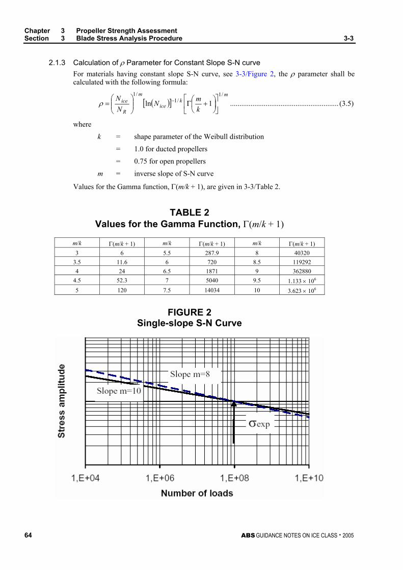
Chapter 3 Propeller Strength Assessment Section 3 Blade Stress Analysis Procedure 3-3
64 ABS GUIDANCE NOTES ON ICE CLASS . 2005
2.1.3 Calculation of ρ Parameter for Constant Slope S-N curve For materials having constant slope S-N curve, see 3-3/Figure 2, the ρ parameter shall be calculated with the following formula:
( )[ ]m
kice
m
R
ice
kmN
NN /1
/1/1
1ln ⎥⎦
⎤⎢⎣
⎡⎟⎠⎞
⎜⎝⎛ +Γ⎟⎟
⎠
⎞⎜⎜⎝
⎛= −ρ .......................................................... (3.5)
where
k = shape parameter of the Weibull distribution
= 1.0 for ducted propellers
= 0.75 for open propellers
m = inverse slope of S-N curve
Values for the Gamma function, Γ(m/k + 1), are given in 3-3/Table 2.
TABLE 2 Values for the Gamma Function, Γ(m/k + 1)
m/k Γ(m/k + 1) m/k Γ(m/k + 1) m/k Γ(m/k + 1) 3 6 5.5 287.9 8 40320
3.5 11.6 6 720 8.5 119292 4 24 6.5 1871 9 362880
4.5 52.3 7 5040 9.5 1.133 × 10⁶
5 120 7.5 14034 10 3.623 × 10⁶
FIGURE 2 Single-slope S-N Curve
Chapter 3 Propeller Strength Assessment Section 3 Blade Stress Analysis Procedure 3-3
ABS GUIDANCE NOTES ON ICE CLASS . 2005 65
2.1.4 Acceptability Criterion for Fatigue The equivalent fatigue stress σfat (Equation 3.2) at all locations on the blade has to fulfill the following acceptability criterion:
5.1≥fat
fl
σσ
............................................................................................................... (3.6)
where
σfl = characteristic fatigue strength of blade material after considering the reduction due to the effects of scatter and test specimen size, variable amplitude loading and mean stress (see Equation 3.4)
2.2 Plastic Failure For plastic failure safety, the following criterion for calculated blade stresses needs to be fulfilled.
3.1≥σ
σ ref ............................................................................................................................ (3.7)
where
σ = calculated stress for the design loads. If FE analysis is used in estimation of the stresses, von Mises stresses should be used.
σref = reference stress, defined as follows:
= min{0.7σu, 0.6σ0.2 + 0.4σu}............................................................................. (3.8)
σu = ultimate stress
σ0.2 = proof stress (or yielding stress)

This Page Intentionally Left Blank
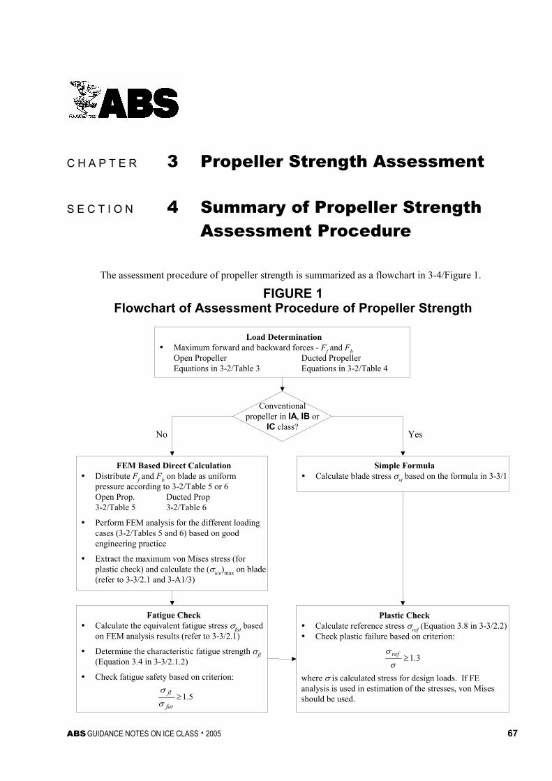
ABS GUIDANCE NOTES ON ICE CLASS . 2005 67
Section 4: Summary of Propeller Strength Assessment Procedure
C H A P T E R 3 Propeller Strength Assessment
S E C T I O N 4 Summary of Propeller Strength Assessment Procedure
The assessment procedure of propeller strength is summarized as a flowchart in 3-4/Figure 1.
FIGURE 1 Flowchart of Assessment Procedure of Propeller Strength
Load DeterminationMaximum forward and backward forces - Ff and FbOpen Propeller Ducted PropellerEquations in 3-2/Table 3 Equations in 3-2/Table 4
Conventionalpropeller in IA, IB or
IC class?
Simple FormulaCalculate blade stress σst based on the formula in 3-3/1
FEM Based Direct CalculationDistribute Ff and Fb on blade as uniformpressure according to 3-2/Table 5 or 6Open Prop. Ducted Prop3-2/Table 5 3-2/Table 6
Perform FEM analysis for the different loadingcases (3-2/Tables 5 and 6) based on goodengineering practice
Extract the maximum von Mises stress (forplastic check) and calculate the (σice)max on blade(refer to 3-3/2.1 and 3-A1/3)
Fatigue CheckCalculate the equivalent fatigue stress σfat basedon FEM analysis results (refer to 3-3/2.1)
Determine the characteristic fatigue strength σfl(Equation 3.4 in 3-3/2.1.2)
Check fatigue safety based on criterion:
5.1≥fat
fl
σσ
Plastic CheckCalculate reference stress σref (Equation 3.8 in 3-3/2.2)Check plastic failure based on criterion:
where σ is calculated stress for design loads. If FEanalysis is used in estimation of the stresses, von Misesshould be used.
3.1≥σσ ref
No Yes

This Page Intentionally Left Blank

ABS GUIDANCE NOTES ON ICE CLASS . 2005 69
Section 5: References
C H A P T E R 3 Propeller Strength Assessment
S E C T I O N 5 References
[1] Finnish Maritime Administration, 2004, ‘Draft Proposal for the Finnish Swedish Ice Class Rules for Propulsion Machinery’.
[2] Koskinen, P. Jussila, M. and Soininen, H. 2004, ‘On the comments received to the “Draft Proposal for the Finnish Swedish Ice Class Rules for Propulsion Machinery”’, Research report no. TUO57-044008, VTT Technical Research Center of Finland.
[3] Koskinen, P. Jussila, M. and Soininen, H. 1996, ‘Propeller Ice Load Models’, Research Notes 1739, VTT Technical Research Center of Finland

This Page Intentionally Left Blank

ABS GUIDANCE NOTES ON ICE CLASS . 2005 71
Appendix 1: Illustrative Example
C H A P T E R 3 Propeller Strength Assessment
A P P E N D I X 1 Illustrative Example
1 Information Required for Blade Strength Check The illustrative example used in this Section is a CPP in IC class. The propeller is designed with a skew angle of 26° and classified as a highly-skewed propeller. The information required for the blade strength check is summarized as follows:
General Ice class: IC Prime mover: Diesel engine Propeller type: Open CPP propeller Number of Blade: 4 Propeller diameter: 6000.0 mm Hub diameter: 1600.0 mm Expanded blade area ratio: 0.525 Propeller rotational speed: 119.0 rpm Design ice thickness: 1.00 m Propeller material: Nickel-aluminum bronze Young's module: 118000. N/mm2 Shear module: 44360. N/mm2 Density: 7.500 g/cm3 Ultimate tensile strength: 590. N/mm2 0.2% proof strength: 245. N/mm2 Propeller movability : Fixing Propeller location : Centerline SN Curve: single slope with m (inverse slope) = 8 Mean fatigue strength (10e8 cycles in sea water): 82.600 N/mm2 Reduction factor (mean stress effect): 0.750 Reduction factor (variable amplitude loading effect): 1.000 Ruduction factor (scatter and test speciment size effect): 1.000 Depth of the propeller centerline from winter waterline: 4.000 Propeller Geometry Number of radii: 12 r/R ---- Pitch ---- ---- Rake ---- ------------- Skew ------------- Width Length Angle Design Total Exp.Len. Exp.GL-LE Len. Angle (mm) (deg.) (mm) (mm) (mm) (mm) (deg.) (mm) 0.275 4348.000 39.990 0.000 0.000 0.000 470.300 0.000 940.600 0.300 4433.000 38.094 0.000 -17.892 -29.000 549.100 -1.453 1040.200 0.350 4590.000 34.828 0.000 -49.144 -86.050 700.900 -3.854 1229.700 0.400 4726.000 32.080 0.000 -74.088 -139.500 842.200 -5.644 1405.400 0.500 4933.000 27.628 0.000 -103.133 -222.400 1077.400 -7.526 1710.000 0.600 5059.000 24.100 0.000 -100.836 -246.950 1217.300 -7.176 1940.700 0.700 5100.000 21.133 0.000 -64.174 -178.000 1215.900 -4.530 2075.800 0.800 4990.000 18.310 0.000 7.147 22.750 1014.300 0.516 2074.100 0.900 4520.000 14.919 0.000 95.143 369.550 546.400 7.578 1831.900 0.950 4111.000 12.930 0.000 148.125 662.000 92.600 12.971 1509.200 0.975 3859.000 11.858 0.000 173.366 843.650 -240.600 16.173 1206.100 1.000 3568.000 10.719 0.000 183.568 987.000 -547.700 18.521 878.600
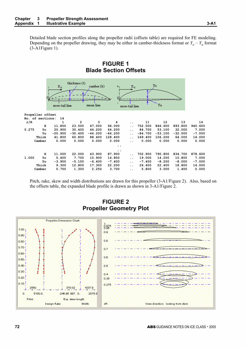
Chapter 3 Propeller Strength Assessment Appendix 1 Illustrative Example 3-A1
72 ABS GUIDANCE NOTES ON ICE CLASS . 2005
Detailed blade section profiles along the propeller radii (offsets table) are required for FE modeling. Depending on the propeller drawing, they may be either in camber-thickness format or Yo – Yu format (3-A1Figure 1).
FIGURE 1 Blade Section Offsets
Propeller offset No. of sections: 14 r/R 1 2 3 4 .. 11 12 13 14 X 11.800 23.500 47.000 94.000 .. 752.500 846.600 893.800 940.600 0.275 Yo 20.900 30.400 44.200 64.200 .. 84.700 53.100 32.000 7.000 Yu -20.900 -30.400 -44.200 -64.200 .. -84.700 -53.100 -32.000 -7.000 Thick 41.800 60.800 88.400 128.400 .. 169.400 106.200 64.000 14.000 Camber 0.000 0.000 0.000 0.000 .. 0.000 0.000 0.000 0.000
..
.. X 11.000 22.000 43.900 87.900 .. 702.900 790.800 834.700 878.600 1.000 Yo 5.400 7.700 10.900 14.800 .. 19.000 14.200 10.800 7.000 Yu -3.900 -5.100 -6.400 -7.400 .. -7.400 -8.200 -8.000 -7.000 Thick 9.300 12.800 17.300 22.200 .. 26.400 22.400 18.800 14.000 Camber 0.750 1.300 2.250 3.700 .. 5.800 3.000 1.400 0.000
Pitch, rake, skew and width distributions are drawn for this propeller (3-A1/Figure 2). Also, based on the offsets table, the expanded blade profile is drawn as shown in 3-A1/Figure 2.
FIGURE 2 Propeller Geometry Plot
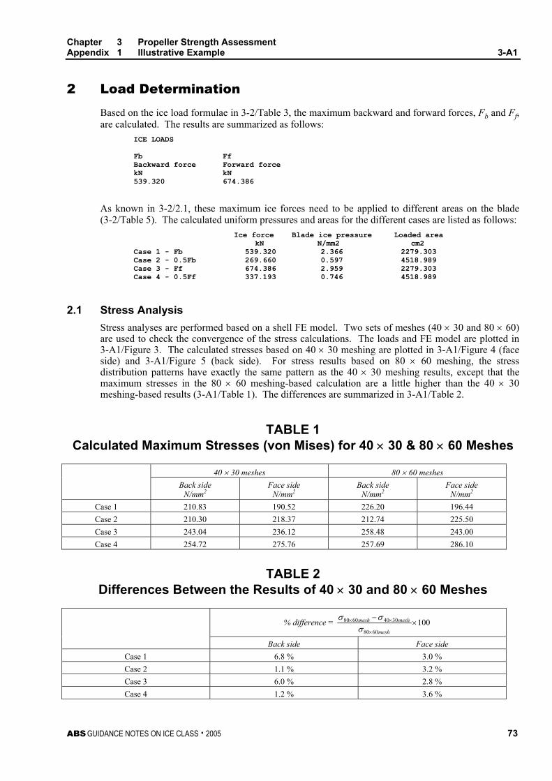
Chapter 3 Propeller Strength Assessment Appendix 1 Illustrative Example 3-A1
ABS GUIDANCE NOTES ON ICE CLASS . 2005 73
2 Load Determination
Based on the ice load formulae in 3-2/Table 3, the maximum backward and forward forces, Fb and Ff, are calculated. The results are summarized as follows:
ICE LOADS Fb Ff Backward force Forward force kN kN 539.320 674.386
As known in 3-2/2.1, these maximum ice forces need to be applied to different areas on the blade (3-2/Table 5). The calculated uniform pressures and areas for the different cases are listed as follows:
Ice force Blade ice pressure Loaded area kN N/mm2 cm2
Case 1 - Fb 539.320 2.366 2279.303 Case 2 - 0.5Fb 269.660 0.597 4518.989 Case 3 - Ff 674.386 2.959 2279.303 Case 4 - 0.5Ff 337.193 0.746 4518.989
2.1 Stress Analysis Stress analyses are performed based on a shell FE model. Two sets of meshes (40 × 30 and 80 × 60) are used to check the convergence of the stress calculations. The loads and FE model are plotted in 3-A1/Figure 3. The calculated stresses based on 40 × 30 meshing are plotted in 3-A1/Figure 4 (face side) and 3-A1/Figure 5 (back side). For stress results based on 80 × 60 meshing, the stress distribution patterns have exactly the same pattern as the 40 × 30 meshing results, except that the maximum stresses in the 80 × 60 meshing-based calculation are a little higher than the 40 × 30 meshing-based results (3-A1/Table 1). The differences are summarized in 3-A1/Table 2.
TABLE 1 Calculated Maximum Stresses (von Mises) for 40 × 30 & 80 × 60 Meshes
40 × 30 meshes 80 × 60 meshes Back side
N/mm2 Face side
N/mm2 Back side
N/mm2 Face side
N/mm2 Case 1 210.83 190.52 226.20 196.44 Case 2 210.30 218.37 212.74 225.50 Case 3 243.04 236.12 258.48 243.00 Case 4 254.72 275.76 257.69 286.10
TABLE 2 Differences Between the Results of 40 × 30 and 80 × 60 Meshes
% difference = 1006080
30406080 ×−
×
××
mesh
meshmesh
σσσ
Back side Face side Case 1 6.8 % 3.0 % Case 2 1.1 % 3.2 % Case 3 6.0 % 2.8 % Case 4 1.2 % 3.6 %

FIG
UR
E 3
Mes
hes
and
Bla
de P
ress
ure
used
in Il
lust
rativ
e Ex
ampl
e
Load
Pre
ssur
e A
reas
FE
M M
eshe
s
Lo
adin
g ar
ea fo
r Cas
e 1
& C
ase
3 (p
ress
ure
is p
lotte
d ba
sed
on C
ase
1)
40
× 3
0 (e
lem
ent #
in ra
dial
dire
ctio
n ×
chor
dwis
e di
rect
ion)
Lo
adin
g ar
ea fo
r Cas
e 2
& C
ase
4 (p
ress
ure
is p
lotte
d ba
sed
on C
ase
2)
80
× 6
0 (e
lem
ent #
in ra
dial
dire
ctio
n ×
chor
dwis
e di
rect
ion)
Chapter 3 Propeller Strength Assessment Appendix 1 Illustrative Example 3-A1
74 ABS GUIDANCE NOTES ON ICE CLASS . 2005

FIG
UR
E 4
Stre
ss (v
on M
ises
) Dis
trib
utio
n on
Bac
k Si
de (4
0 ×
30 M
eshe
s)
C
ase
1: S
tress
dis
tribu
tion
on b
ack
side
Cas
e 2:
Stre
ss d
istri
butio
n on
bac
k si
de
C
ase
3: S
tress
dis
tribu
tion
on b
ack
side
Cas
e 4:
Stre
ss d
istri
butio
n on
bac
k si
de
Chapter 3 Propeller Strength Assessment Appendix 1 Illustrative Example 3-A1
ABS GUIDANCE NOTES ON ICE CLASS . 2005 75

FIG
UR
E 5
Stre
ss (v
on M
ises
) Dis
trib
utio
n on
Fac
e Si
de (4
0 ×
30 M
eshe
s)
C
ase
1: S
tress
dis
tribu
tion
on fa
ce si
de
C
ase
2: S
tress
dis
tribu
tion
on fa
ce si
de
C
ase
3: S
tress
dis
tribu
tion
on fa
ce si
de
C
ase
4: S
tress
dis
tribu
tion
on fa
ce si
de
Chapter 3 Propeller Strength Assessment Appendix 1 Illustrative Example 3-A1
76 ABS GUIDANCE NOTES ON ICE CLASS . 2005

Chapter 3 Propeller Strength Assessment Appendix 1 Illustrative Example 3-A1
ABS GUIDANCE NOTES ON ICE CLASS . 2005 77
3 Blade Strength Check
Stress criteria have already been described in 3-3/2.1 and 3-3/2.2 based on the Finnish Swedish Ice Class Rules. In this Subsection, the calculation of equivalent fatigue stress, σfat, will be further explained based on our understanding.
According to the Ice Class Rules, the equivalent fatigue stress, σfat, is calculated as:
σfat = ρ × (σice)max
where
(σice)max = mean value of the principal stress amplitudes due to the design forward and backward blade forces at the studied location.
= 0.5[(σice)fmax – (σice)bmax]
(σice)fmax = principal stress due to forward load
(σice)bmax = principal stress due to backward load
It should be noted that in calculating (σice)max, the values of (σice)fmax and (σice)bmax should be based on an approximately same location. In the loading conditions of Cases 1, 2, 3 and 4 required by the FSICR for the current study case, only Case 1 and Case 3 (similar to Case 2 and Case 4) can match as a pair to generate a maximum (σice)fmax and (σice)bmax pair approximately at a nearby location (see 3-A1/Figure 6 and 7). The pairs used in the calculation of (σice)max are summarized in the following table.
TABLE 3 Calculation of (σice)max
Pair: Case 1 & Case 3 (σice)max = max{(σice)max-face, (σice)max-back}
Face side mean value of the principal stress amplitudes
Back side mean value of the principal stress amplitudes
(σice)max-face
major (σice)fmax (Case 3) – minor (σice)bmax (Case 1)
(σice)max-back
major (σice)bmax (Case 1) – minor (σice)fmax (Case 3)
Pair: Case 2 & Case 4 (σice)max = max{(σice)max-face, (σice)max-back}
Face side mean value of the principal stress amplitudes
Back side mean value of the principal stress amplitudes
(σice)max-face
major (σice)fmax (Case 4) – minor (σice)bmax (Case 2)
(σice)max-back
major (σice)bmax (Case 2) – minor (σice)fmax (Case 4)
The final values of (σice)max in the Case 1-3 pair and the Case 2-4 pair are based on the maximum values of face and back sides (σice)max = max{(σice)max-face, (σice)max-back}.

FIG
UR
E 6
Prin
cipa
l Str
ess
Dis
trib
utio
n on
Bac
k Si
de (8
0 ×
60 M
eshe
s)
C
ase
1: P
rinci
pal s
tress
dis
tribu
tion
on b
ack
side
Cas
e 2:
Prin
cipa
l stre
ss d
istri
butio
n on
bac
k si
de
C
ase
3: P
rinci
pal s
tress
dis
tribu
tion
on b
ack
side
Cas
e 4:
Prin
cipa
l stre
ss d
istri
butio
n on
bac
k si
de
Chapter 3 Propeller Strength Assessment Appendix 1 Illustrative Example 3-A1
78 ABS GUIDANCE NOTES ON ICE CLASS . 2005

FIG
UR
E 7
Prin
cipa
l Str
ess
Dis
trib
utio
n on
Fac
e Si
de (8
0 ×
60 M
eshe
s)
C
ase
1: P
rinci
pal s
tress
dis
tribu
tion
on fa
ce si
de
C
ase
2: P
rinci
pal s
tress
dis
tribu
tion
on fa
ce si
de
C
ase
3: P
rinci
pal s
tress
dis
tribu
tion
on fa
ce si
de
C
ase
4: P
rinci
pal s
tress
dis
tribu
tion
on fa
ce si
de
Chapter 3 Propeller Strength Assessment Appendix 1 Illustrative Example 3-A1
ABS GUIDANCE NOTES ON ICE CLASS . 2005 79

Chapter 3 Propeller Strength Assessment Appendix 1 Illustrative Example 3-A1
80 ABS GUIDANCE NOTES ON ICE CLASS . 2005
According to the aforementioned matching pairs, the equivalent fatigue stresses are calculated. The fatigue failure check results are summarized as follows: FATIGUE CHECK Fatigue strength Equivalent fatigue stress Safety factor σfl σfat σfl/σfat N/mm2 N/mm2 >=1.5 40×30 meshing Case 1-3 pair 61.940 35.830 1.728 Case 2-4 pair 61.940 37.090 1.670 80×60 meshing Case 1-3 pair 61.940 38.340 1.615 Case 2-4 pair 61.940 37.470 1.653
For the plastic failure check, the criterion described in 3-3/2.2 is used and results are given as follows: PLASTIC FAILURE CHECK Reference stress Calculated stress (Von Mises) Safety factor σref σ σ/σref N/mm2 N/mm2 >=1.3 40×30 meshing Case 1 383.000 210.830 1.816 Case 2 383.000 218.370 1.753 Case 3 383.000 243.040 1.575 Case 4 383.000 275.750 1.388 80×60 meshing Case 1 383.000 226.200 1.693 Case 2 383.000 225.490 1.698 Case 3 383.000 258.480 1.481 Case 4 383.000 286.090 1.338
As both fatigue and plastic failure criteria are satisfied, the propeller under review is concluded to be strength safe.