Guidance Material and Best Practices for Inventory Management ...
155
Guidance Material and Best Practices for Inventory Management 2nd Edition
Transcript of Guidance Material and Best Practices for Inventory Management ...

Guidance Material and Best Practices for Inventory Management
2nd Edition

Guidance Material and Best Practices for Inventory ManagementISBN 978-92-9252-741-9© 2015 International Air Transport Association. All rights reserved.Montreal—Geneva
NOTICEDISCLAIMER. The information contained in this publication is subject to constant review in the light of changing government requirements and regula-tions. No subscriber or other reader should act on the basis of any such information without referring to applicable laws and regulations and/or without taking appropriate professional advice. Although every effort has been made to ensure accuracy, the International Air Transport Association shall not be held responsible for any loss or damage caused by errors, omissions, misprints or misinterpretation of the contents hereof. Furthermore, the International Air Transport Association expressly disclaims any and all liability to any person or entity, whether a purchaser of this publication or not, in respect of anything done or omitted, and the consequences of anything done or omitted, by any such person or entity in reliance on the contents of this publication.
© International Air Transport Association. All Rights Reserved. No part of this publication may be reproduced, recast, reformatted or trans-mitted in any form by any means, electronic or mechanical, including photocopying, record-ing or any information storage and retrieval sys-tem, without the prior written permission from:
Senior Vice PresidentSafety and Flight Operations
International Air Transport Association800 Place Victoria
P.O. Box 113Montreal, Quebec
CANADA H4Z 1M1

2nd
Edition 2015 i
Table of Content
List of Figures .................................................................................................................................................. v
List of Tables ..................................................................................................................................................vii
Abbreviations ................................................................................................................................................viii
Introduction ...................................................................................................................................................... x
Purpose of the Guide .....................................................................................................................................xi
Scope ............................................................................................................................................................ xi
Audience ....................................................................................................................................................... xi
Objective ...................................................................................................................................................... xii
Section 1—Goals of Inventory Management ................................................................................................ 1
Section 2—Introduction to Inventory Classification .................................................................................... 4
2.1 Rotable Inventory ............................................................................................................................... 8
2.2 Repairable Inventory .......................................................................................................................... 9
2.3 Expendable Inventory ......................................................................................................................10
2.4 Recoverable Inventory .....................................................................................................................11
2.5 SPEC2000 Inventory Classification .................................................................................................12
2.5.1 SPC 1 ...........................................................................................................................................12
2.5.2 SPC 2 ...........................................................................................................................................12
2.5.3 SPC 6 ...........................................................................................................................................12
Section 3—Initial Discussion of Airline Provisioning ................................................................................13
3.1 Sources for Spares Provisioning Data .............................................................................................16
3.1.1 Data from the Aircraft Manufacturer ............................................................................................16
3.1.2 Operational Data from another Carrier with the Same or Similar Fleet .......................................22
3.1.3 Data from an MRO Partnering with the Carrier for Spares Provisioning and Repair/Overhaul ...22
3.1.4 Data from Industry Experts or Consultants ..................................................................................22
3.2 How to Provision for Airline Operations ...........................................................................................23
3.2.1 Nine Step Model to Determine ROTABLE Inventory Support for Airline Operations ..................23
3.2.2 Understand Airline Operational Goals .........................................................................................24
3.2.3 Gather Needed Data ....................................................................................................................24
3.2.4 Calculate Annual Demand ...........................................................................................................26
3.2.5 Designate Stock Items .................................................................................................................27
3.2.6 Calculate Station Qualification .....................................................................................................28
Guidance Material and Best Practices for Inventory Management
ii 2nd
Edition 2015
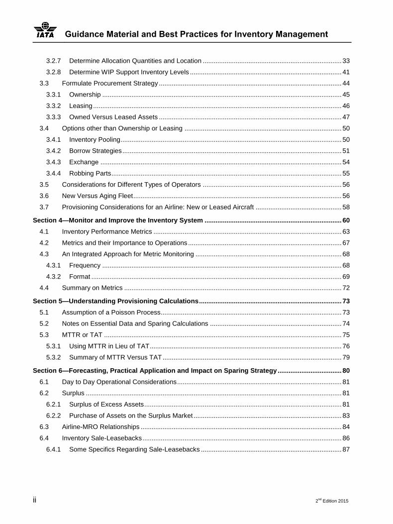
3.2.7 Determine Allocation Quantities and Location ............................................................................ 33
3.2.8 Determine WIP Support Inventory Levels ................................................................................... 41
3.3 Formulate Procurement Strategy .................................................................................................... 44
3.3.1 Ownership ................................................................................................................................... 45
3.3.2 Leasing ........................................................................................................................................ 46
3.3.3 Owned Versus Leased Assets .................................................................................................... 47
3.4 Options other than Ownership or Leasing ...................................................................................... 50
3.4.1 Inventory Pooling ......................................................................................................................... 50
3.4.2 Borrow Strategies ........................................................................................................................ 51
3.4.3 Exchange .................................................................................................................................... 54
3.4.4 Robbing Parts .............................................................................................................................. 55
3.5 Considerations for Different Types of Operators ............................................................................ 56
3.6 New Versus Aging Fleet .................................................................................................................. 56
3.7 Provisioning Considerations for an Airline: New or Leased Aircraft ............................................... 58
Section 4—Monitor and Improve the Inventory System ........................................................................... 60
4.1 Inventory Performance Metrics ....................................................................................................... 63
4.2 Metrics and their Importance to Operations .................................................................................... 67
4.3 An Integrated Approach for Metric Monitoring ................................................................................ 68
4.3.1 Frequency ................................................................................................................................... 68
4.3.2 Format ......................................................................................................................................... 69
4.4 Summary on Metrics ....................................................................................................................... 72
Section 5—Understanding Provisioning Calculations .............................................................................. 73
5.1 Assumption of a Poisson Process ................................................................................................... 73
5.2 Notes on Essential Data and Sparing Calculations ........................................................................ 74
5.3 MTTR or TAT .................................................................................................................................. 75
5.3.1 Using MTTR in Lieu of TAT ......................................................................................................... 76
5.3.2 Summary of MTTR Versus TAT .................................................................................................. 79
Section 6—Forecasting, Practical Application and Impact on Sparing Strategy ................................... 80
6.1 Day to Day Operational Considerations .......................................................................................... 81
6.2 Surplus ............................................................................................................................................ 81
6.2.1 Surplus of Excess Assets ............................................................................................................ 81
6.2.2 Purchase of Assets on the Surplus Market ................................................................................. 83
6.3 Airline-MRO Relationships .............................................................................................................. 84
6.4 Inventory Sale-Leasebacks ............................................................................................................. 86
6.4.1 Some Specifics Regarding Sale-Leasebacks ............................................................................. 87

Table of Content
2nd
Edition 2015 iii
Section 7—Optimization of Airline Inventory .............................................................................................89
7.1 Goals Revisited with Optimization ...................................................................................................91
7.1.1 Organizational Structures ............................................................................................................92
7.2 Interactions an Inventory Manager Should Expect ..........................................................................95
7.2.1 Internal Interactions .....................................................................................................................95
7.2.2 External Interactions ....................................................................................................................98
7.3 Expendable Planning .......................................................................................................................99
7.3.1 Introduction ..................................................................................................................................99
7.3.2 Expendable Planning Strategies ................................................................................................100
7.3.3 Planning the Expendables Warehouse .....................................................................................105
7.3.4 Planning Station Expendables ...................................................................................................107
7.3.4.1 Data Needed ......................................................................................................................108
7.3.4.2 Calculating Safety Stock ....................................................................................................108
7.3.5 Planning the Station ...................................................................................................................110
7.3.5.1 Determine Stock Items ......................................................................................................111
7.3.5.2 Determine Replenishment Lead Time ...............................................................................112
7.3.5.3 Set Allocation Quantity ......................................................................................................112
7.3.5.4 Set Safety Stock or Min .....................................................................................................113
7.3.5.5 Determine Reorder Point ...................................................................................................113
7.3.6 Planning the Warehouse ...........................................................................................................115
7.3.6.1 Minimum Lot Sizes.............................................................................................................116
7.3.6.2 Basic Inventory Model .......................................................................................................116
7.3.6.3 Safety Stock at the Warehouse .........................................................................................117
7.3.6.4 Calculating the Safety Stock and Reorder Points at the Warehouse ................................118
7.4 MRP/ERP in Warehouse Management .........................................................................................121
7.4.1 EOQ in Warehouse Management..............................................................................................122
7.4.2 Discussion of Ordering Strategies .............................................................................................123
7.4.2.1 Planning for the Hangar Bay ..............................................................................................125
7.4.2.2 Control of Expendable Inventories .....................................................................................125
7.4.2.3 Inventory Accuracy ............................................................................................................126
Section 8—Accounting for Rotables and Expendables ..........................................................................127
8.1 Introduction ....................................................................................................................................127
8.2 Rotables .........................................................................................................................................127
8.3 Expendables/Consumables ...........................................................................................................128
8.4 Accounting Summary .....................................................................................................................130

Guidance Material and Best Practices for Inventory Management
iv 2nd
Edition 2015
Section 9—New Value Chain Options ....................................................................................................... 131
9.1 Point-of-Use Trends ...................................................................................................................... 131
9.2 Distributive Versus Allocated Models ............................................................................................ 131
Section 10—Inventory Assessment .......................................................................................................... 134
10.1 OECM ............................................................................................................................................ 134
10.2 Recommendation and Examples .................................................................................................. 135
10.2.1 Recommendation .................................................................................................................. 135
10.2.2 Examples ............................................................................................................................... 136
Section 11—Work Cited .............................................................................................................................. 138
Section 12—Acknowledgements ............................................................................................................... 139

List of Figures
2nd
Edition 2015 v
List of Figures
Figure 1. Goal Hierarchy in Aviation Inventory Management........................................................................ 3
Figure 2. Inventory Classifications and Characteristics ................................................................................ 4
Figure 3. Examples of Commonly Allocated Parts by Material Type ............................................................ 5
Figure 4. Aircraft, Airframe, and Engine Inventory ........................................................................................ 6
Figure 5. QEC and LRU Inventory Relationship to Engine and Airframe Inventory ..................................... 8
Figure 6. High Level Inventory System Design ...........................................................................................13
Figure 7. Nine Step Inventory Provisioning Model ......................................................................................24
Figure 8. Situations with Potential for Inventory Consolidation ...................................................................34
Figure 9. Critical Path of Remove and Install ..............................................................................................36
Figure 10. Representation of the Removal and Repair Cycle Showing the Repair Pipeline ........................39
Figure 11. Provisioning Options Summarized ...............................................................................................55
Figure 12. Typical Bathtub Curve ..................................................................................................................57
Figure 13. Flow of Inventory through the Airline ...........................................................................................60
Figure 14. SIPOC Model ...............................................................................................................................60
Figure 15. Detailed SIPOC model .................................................................................................................61
Figure 16. Typical Six Sigma DMAIC Cycle ..................................................................................................62
Figure 17. Pareto Chart for Monthly No-Fills by Station ................................................................................70
Figure 18. Pareto Chart for Normalized Station Data ...................................................................................71
Figure 19. Run Chart - Station 3 No Fills, Rolling 12 months .......................................................................72
Figure 20. Right Skewed Distribution ............................................................................................................76
Figure 21. Left Skewed Distribution ..............................................................................................................77
Figure 22. Symmetric Distribution .................................................................................................................78
Figure 23. A Multimodal Distribution .............................................................................................................78
Figure 24. Comparison of Inventory Investment to DL/CX ............................................................................89
Figure 25. Internal Interactions ......................................................................................................................95
Figure 26. External Interactions ....................................................................................................................99
Figure 27. Demand from outstations required from Warehouse .................................................................103
Figure 28. Expendable Planning Simplified.................................................................................................107
Figure 29. Setting up Stations or Warehouse First? ...................................................................................107
Figure 30. Examples of Line Maintenance Events Driving Expendable Demand .......................................109
Figure 31. Kitting Best Practices .................................................................................................................110
Figure 32. Inventory and Maintenance Daily Cycle .....................................................................................114
Figure 33. Inventory Model for Expendables...............................................................................................116

Guidance Material and Best Practices for Inventory Management
vi 2nd
Edition 2015
Figure 34. Actual Demand Pattern ............................................................................................................. 117
Figure 35. Accountable and Non-Accountable Stations ............................................................................. 129
Figure 36. Daily Cycle of a Distributive Model ............................................................................................ 133
Figure 37. Rotable Balance ........................................................................................................................ 137
List of Tables
2nd
Edition 2015 vii
List of Tables
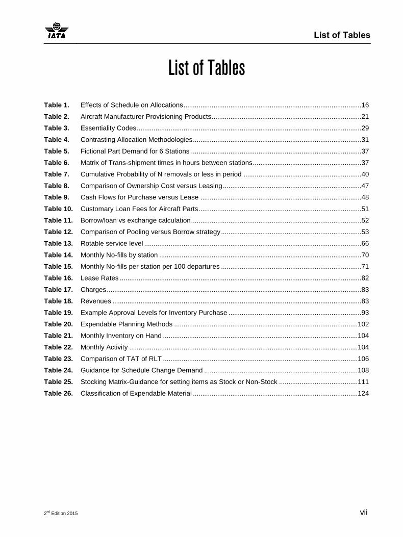
Table 1. Effects of Schedule on Allocations ...............................................................................................16
Table 2. Aircraft Manufacturer Provisioning Products ................................................................................21
Table 3. Essentiality Codes ........................................................................................................................29
Table 4. Contrasting Allocation Methodologies ..........................................................................................31
Table 5. Fictional Part Demand for 6 Stations ...........................................................................................37
Table 6. Matrix of Trans-shipment times in hours between stations ..........................................................37
Table 7. Cumulative Probability of N removals or less in period ...............................................................40
Table 8. Comparison of Ownership Cost versus Leasing ..........................................................................47
Table 9. Cash Flows for Purchase versus Lease ......................................................................................48
Table 10. Customary Loan Fees for Aircraft Parts .......................................................................................51
Table 11. Borrow/loan vs exchange calculation ...........................................................................................52
Table 12. Comparison of Pooling versus Borrow strategy ...........................................................................53
Table 13. Rotable service level ....................................................................................................................66
Table 14. Monthly No-fills by station ............................................................................................................70
Table 15. Monthly No-fills per station per 100 departures ...........................................................................71
Table 16. Lease Rates .................................................................................................................................82
Table 17. Charges ........................................................................................................................................83
Table 18. Revenues .....................................................................................................................................83
Table 19. Example Approval Levels for Inventory Purchase .......................................................................93
Table 20. Expendable Planning Methods ..................................................................................................102
Table 21. Monthly Inventory on Hand ........................................................................................................104
Table 22. Monthly Activity ..........................................................................................................................104
Table 23. Comparison of TAT of RLT ........................................................................................................106
Table 24. Guidance for Schedule Change Demand ..................................................................................108
Table 25. Stocking Matrix-Guidance for setting items as Stock or Non-Stock ..........................................111
Table 26. Classification of Expendable Material ........................................................................................124

Guidance Material and Best Practices for Inventory Management
viii 2nd
Edition 2015
Abbreviations
ASPL
ADVANCED SPARE PARTS LIST
AD
ADVISORY DIRECTIVE
ATC
AIR TRAFFIC CONTROL
ATA
AIR TRANSPORT AUTHORITY
A/C
AIRCRAFT
AOG
AIRCRAFT ON GROUND
ACOOS
AIRCRAFT OUT OF SERVICE
APU
AUXILIARY POWER UNIT
BKO
BACKORDERS
BOM
BILL OF MATERIAL
CX
CANCELLATION
CLP
CATALOGUE LIST PRICE
CMM
COMPONENT MAINTENANCE MANUAL
DD
DAILY DEMAND
DL
DELAY
EOQ
ECONOMIC ORDER QUANTITY
EO
ENGINEERING ORDER
ERP
ENTERPRICE RESOURCE PLANNING
ETOPS
EXTENDED-RANGE TWIN-ENGINE OPERATIONS
FMV
FAIR MARKET VALUE
FIFO
FIRST IN FIRST OUT
FAK
FLY AWAY KIT
FOD
FOREIGN OBJECT DAMAGE
ID
IDENTICALLY DISTRIBUTED
IPC
ILLUSTRATED PARTS CATALOUGE
IT
INFORMATION TECHNOLOGY
IATP
INTERNATIONAL AIRLINE TECHNICAL POOLING
IROPS
IRREGULAR OPERATION
JIT
JUST IN TIME
LTF
LEAD TIME FACTOR
LLP
LIFE LIMITED PART
LRU
LINE REPLACEABLE UNIT
MCO
MAINTENANCE CARRY OVER
MCC
MAINTENANCE CONTROL CENTER
MRO
MAINTENANCE REPAIR & OVERHAUL
MPN
MANUFACTURER PART NUMBER
Abbreviations
2nd
Edition 2015 ix
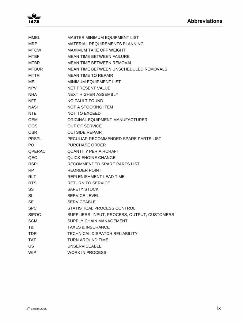
MMEL
MASTER MINIMUM EQUIPMENT LIST
MRP
MATERIAL REQUIREMENTS PLANNING
MTOW
MAXIMUM TAKE OFF WEIGHT
MTBF
MEAN TIME BETWEEN FAILURE
MTBR
MEAN TIME BETWEEN REMOVAL
MTBUR
MEAN TIME BETWEEN UNSCHEDULED REMOVALS
MTTR
MEAN TIME TO REPAIR
MEL
MINIMUM EQUIPMENT LIST
NPV
NET PRESENT VALUE
NHA
NEXT HIGHER ASSEMBLY
NFF
NO FAULT FOUND
NASI
NOT A STOCKING ITEM
NTE
NOT TO EXCEED
OEM
ORIGINAL EQUIPMENT MANUFACTURER
OOS
OUT OF SERVICE
OSR
OUTSIDE REPAIR
PRSPL
PECULIAR RECOMMENDED SPARE PARTS LIST
PO
PURCHASE ORDER
QPERAC
QUANTITY PER AIRCRAFT
QEC
QUICK ENGINE CHANGE
RSPL
RECOMMENDED SPARE PARTS LIST
RP
REORDER POINT
RLT
REPLENISHMENT LEAD TIME
RTS
RETURN TO SERVICE
SS
SAFETY STOCK
SL
SERVICE LEVEL
SE
SERVICEABLE
SPC
STATISTICAL PROCESS CONTROL
SIPOC
SUPPLIERS, INPUT, PROCESS, OUTPUT, CUSTOMERS
SCM
SUPPLY CHAIN MANAGEMENT
T&I
TAXES & INSURANCE
TDR
TECHNICAL DISPATCH RELIABILITY
TAT
TURN AROUND TIME
US
UNSERVICEABLE
WIP
WORK IN PROCESS

Guidance Material and Best Practices for Inventory Management
x 2nd
Edition 2015
Introduction
Provisioning of inventory assets is one of the most important factors in successful airline operations,
however sometimes it is one of the least understood. Proper provisioning of inventory assets ensures
adequate coverage in the assured eventuality of a maintenance event requiring a replacement part. These
maintenance events can occur during daily operations (failure or damage) or during a scheduled
maintenance visit. While different in nature, each of these events shares the facet of disruption to airline
operations. During the flight day the disruption may include a late departure or cancellation, and during a
scheduled maintenance event, a removal could jeopardize the work flow and timely return of the aircraft to
service. This guide will strive to provide cost-effective and practical solutions that optimize the provisioning
process and resultant output to airline operations.
Provisioning, or Sparing as it is often called, not only takes into account the facts surrounding removal of a
part, but also the maintenance cycle required to return the removed asset to serviceable condition. The level
of spares required for an operation depends upon numerous factors, including but not limited to operational
or reliability goals, financial factors, removal rates for scheduled and unscheduled removals, repair
turnaround time (TAT) at the vendor or maintenance facility repairing the removed assets, scrap rates for
the removed asset, replenishment lead times for replacement assets, flight schedules, freight options, and a
host of other factors. In addition, there are numerous methods to acquire a spare needed to send an aircraft
back into flight operations. These options include ownership strategies, leasing from a provider, borrowing
from other airlines, spot purchase, spot lease, and exchange of like items with repair or asset vendors. In
this guide we will explore the relevant issues regarding inventory and offer recommendations and
techniques for use both in airline and cargo flight operations that will optimize the airline inventory strategy.

Purpose of the Guide
2nd
Edition 2015 xi
Purpose of the Guide
The intent of this guide is to provide a set of strategies and techniques that will guide an inventory manager
to an optimal inventory solution for a variety of passenger airline and cargo operations. While evaluating the
passenger airline or cargo operations in question, the inventory professional should be able to select the
optimal inventory strategy or blend of inventory strategies that will achieve the operational and financial
goals set by the firm.
Scope
The scope of this document ranges from initial provisioning for a start-up operation, to evaluating and
improving operations of an existing carrier. Topics covered include:
Goals for Airline Inventory Management
Types of Inventory
Discussion of Airline Provisioning
Inventory Performance Metrics
Understanding Provisioning Calculations
Station Allocation
Day-to-Day Operational Considerations
Surplus Inventory
Airline-MRO Relationships
Sale-Leaseback
Optimization Discussions
Organizational Structures
Audience
This guide is intended for use by an aviation professional tasked with finding solutions for inventory
provision. Ideally, an approach should be taken that financially and operationally optimizes the inventory
asset pool. A properly structured inventory strategy will efficiently meet corporate reliability goals by
optimizing the assets within the spare pool. This guide is also intended to be applicable equally to cargo or
passenger operations, large or small, international or domestic, and regardless of aircraft type.
This guide is also intended for use as an introductory material for professionals not normally tasked with
material management responsibilities but who desire a greater understanding of the provisioning process.

Guidance Material and Best Practices for Inventory Management
xii 2nd
Edition 2015
For example, finance professionals or supply chain managers who work closely with material management
organizations may benefit from increased understanding of the principles outlined in this guide.
Objective
After reading this guide, the aviation inventory professional should be prepared to make decisions regarding
inventory provisioning which lead to an optimal solution.

2nd
Edition 2015 1
Section 1—Goals of Inventory Management
In its most fundamental form, the goal of airline inventory management is to provide the highest possible
level of service at the lowest total cost. This tenet applies whether the inventory manager is tasked with
maximizing aircraft and system availability for a scheduled service passenger or cargo airline, or charter
operations. It applies whether the operator has a few aircraft or hundreds and it applies whether the operator
is flying charter operations at a moment’s notice, point-to-point scheduled flights, or a complex network of
domestic and international routes.
While each inventory manager may face slightly different sets of operational characteristics, the goals of
inventory management largely remain the same. At a high level, goals range from preventing delays and
cancellations by ensuring part availability and access for maintenance personnel, to ensuring that fill rates
are adequate to ensure that passenger convenience items have adequate stock so failures of items can be
rapidly addressed by maintenance.
The paramount goal of airline inventory management is to prevent as many cancellations as possible by
adopting a cost effective inventory provisioning, allocation and management system. Cancellations not only
result in lack of service from the origination point, but also impact subsequent departures, perhaps with
catastrophic consequences for the daily schedule. Cancellations due to parts shortage almost always occur
on No-Go items as large as engines down to the smallest flight-critical part.
In addition to preventing cancellation of flights via the application of an inventory management system, an
inventory manager seeks to prevent as many material related delays as possible. This second goal is almost
implied in the first, however, passengers are sensitive to delays, even short delays, as many schedule their
flights based on connecting from one airline to another, or even within the same airline with short layovers.
For point-to-point carriers, preventing delays is essential in maximizing aircraft availability for latter day
operations. A single short delay could cascade into a series of schedule havoc inducing delays and
cancellations at subsequent stations. For charter operators, minimizing delays is essential so that aircraft
availability is maximized during the day for sale to customers. For cargo operators, the considerations are
the same as for passenger airlines. Although most freight (except perishable items) is generally not
adversely affected by delays, the cargo operator’s schedule and aircraft utilization suffer just the same as a
passenger airline, and the cargo operator’s shipping and receiving human customers are certainly sensitive
to a disruption in the flow of their freight.
Prevention of both delays and cancellations serves the airline by delivering aircraft into the schedule on a
consistent basis. For almost all scheduled service, aircraft free of maintenance issues are essential for
profitable operations, regardless of whether the airline carries passengers, cargo or both. In the case of
charter operators, the goal remains the same, and maintaining a high state of readiness is a key to
generating business when opportunities present themselves.
A typical third goal of an airline inventory manager is to provide for a service level of parts availability to the
maintenance function of the airline. Inventory service level or “Fill Rate” coupled with efficient maintenance
Guidance Material and Best Practices for Inventory Management
2 2nd
Edition 2015
practices ensures the aircraft is delivered to the customer in a high state of readiness. Properly managed
inventory also ensures that the human capital of maintenance personnel is efficiently utilized. Low fill rates
can adversely affect operations and customer experience. If an airline has a poor fill rate on items commonly
referred to Minimum Equipment List, or MEL, the operations of the aircraft can be severely hampered. An
example would be passenger seats locked out due to damaged parts needing replacement, forgoing
revenue and resulting in fewer passengers carried to their destination each day until the seat is repaired.
Some parts placed on Deferred Maintenance list or Maintenance Carry Over may temporarily suspend
Extended-range Twin-engine Operational Performance Standards (ETOPS) and will hamper aircraft
operations until the part is replaced. Other items may be passenger convenience items such as reading
lights, or perhaps one lavatory is locked out for a flight, but these items will definitely impact the passenger
experience and perhaps result in customer ill-will and negatively impact repeat business.
A whole new class of goals is related to financial targets. Financials often form the basis of inventory
management (see Figure 1). If money were no object, the job of provisioning for aircraft operations would be
quite simple, if not extremely expensive and wasteful. However, almost all operators impose some type of
limitation on the annual spend for inventory purchase. Most airlines work under sometimes complex budgets
of inventory purchase, scrap, balance growth, surplus goals, etc. Often the inventory manager will be tasked
with a series of financial goals which seem at odds with the notion of providing a high service level. For
example, a manager might be under financial pressure to reduce inventory balance by annually relegating
some portion of inventory to surplus, while simultaneously expanding operations into several new
international stations.

Goals of Inventory Management
2nd
Edition 2015 3
Figure 1. Goal Hierarchy in Aviation Inventory Management
Some other financial goals an inventory manager may face include inventory turns, total balance, balance
growth, and perhaps an investing budget or cash flow metric. Typically in budget year planning, these goals
are set by the financial team and either given to the inventory manager, or in some cases the inventory and
finance teams work collaboratively to set the coming years’ financial goals.
Considering that a modern aircraft can contain a million or more unique part numbers, many in multiple
quantities per aircraft (QPERAC), an inventory manager faces a daunting task. Furthermore, an inventory
manager is often faced with what seem to be conflicting operational and financial goals. However, once
reduced to its most basic form, the goal of airline inventory management is to provide the highest possible
service level at the lowest possible cost.
As we shall see, there are a myriad of tools, techniques, strategies and tactics for achieving what may seem
to be hopelessly conflicted goals. In addition, we shall offer communication suggestions for the inventory
manager to use in discussing goals and results with financial and operational customers. In order to meet
the financial and operational goals, an inventory manager should adopt mind set of optimization for a
system. Once the inventory manager can accept that the performance of the system as a whole is the
proper measurement, and more importantly convince his or her supervisor and customers that such is the
case, providing the highest possible service at the lowest possible cost is certainly an attainable goal.
Delay
Service Level (MEL, Passenger Convenience Items)
Fill Rate (all other inventory)
Financial Goals
Most Operational
Impact
Less Operational
Impact
Cancellation

Guidance Material and Best Practices for Inventory Management
4 2nd
Edition 2015
Section 2—Introduction to Inventory Classification The definition of an airframe inventory is all inventory on the aircraft apart from the engine inventory,
fuselage, flight controls, landing gears, APU etc. Generally air carriers classify airframe inventory into three
types: Rotable Inventory, Repairable Inventory, and Expendable Inventory. There are three main distinctions
between these three types of inventory (see Figure 2: Inventory Classifications and Characteristics). The
first and most definitive distinction is related to scrap rate. Typically Rotables have a very low or even
negligible scrap rate and Repairables will have a scrap rate that must be considered in spares calculations,
contracts, and other planning activities. Expendables will have a 100% scrap rate as they are consumed at
the point of use and upon removal must be discarded. Scrap rate is often the key determinant in deciding
how to classify an item.
The second distinction is financial. Rotables and often Repairables are regarded by airlines as assets and
therefore are treated as such from an accounting perspective. These assets will be held on a firm’s books
and depreciated on a schedule appropriate for the asset and its parent aircraft lifespan. Expendables are
often considered assets while they are held at a central warehouse or main base, however, once issued,
they are expensed to the location receiving the Expendables. Expendables may also be held as assets until
consumed at the point of use then expensed to the department which installed or consumed the
Expendable.
Figure 2. Inventory Classifications and Characteristics
Scrap
Rate
Negligible
Between 0% and 100%
100%, one time use
Financial
Asset, held on firm’s
books until surplus or
scrap
Consumable, expensed at time of issue
Life-cycle
Indefinite
Persists until scrap
Consumed at time of use
Rotable
Repairable
Expendable
Inventory Classification
Inventory Characteristics

Introduction to Inventory Classification
2nd
Edition 2015 5
The third distinction in classifying inventory is the life-cycle characteristic. Closely related to scrap rate, the
life-cycle refers to the durability and persistence of a component once it is purchased. Rotables are
considered to be indefinitely Repairable and often persist in inventory until they are placed in surplus at fleet
retirement. With low scrap rates they can endure many years of operation, with the same asset moving
through the repair and overhaul process many times. Repairables are limited in their durability as an asset
by their scrap rate, and a certain percentage of Repairables will be continually replaced according to their
scrap rate in the repair process. As an example, consider two fictional components, one Repairable, and
one Rotable. Consider that each has an identical failure rate (MTBF-Mean Time Between Failure) to the
other. Consider also that each will be removed on average, four (4) times a year from the operating fleet.
The Rotable has a negligible scrap rate. The Repairable has a 25% scrap rate, meaning that on average
one of the four annual removals will be scrapped in the shop repair process and replaced via an inventory
purchase. The fleet is mature and has been operating for many years. Consider also that the operator owns
four (4) each of the Repairable and four (4) each of the Rotable. After four years, it is reasonable to expect
that every one of the four Repairables in inventory at the beginning of year one has been replaced due to
scrap. However, we would also expect that all four of the Rotables owned at the beginning of year one are
still in inventory. Furthermore, there have been 16 repairs or overhauls accomplished on the Rotables over
the four year period while in comparison, there have been 12 repairs or overhauls completed on the
Repairables, and four scrap replacements, although there were an identical 16 shop visits. Expendables of
course are consumed once they are installed and so persist in inventory only until they are installed.
Additionally Rotables and Repairables can also be distinct in that Rotables are more often tracked, meaning
that the components accumulate hours and cycles while Repairables are issued at time of use and most
often not tracked during their time installed in regards to hours and cycles. A maintenance computer system
might be setup as a Rotable component requiring a component change to be completed in the system while
the Repairable will only require an issue out of the inventory but no component change.
Figure 3. Examples of Commonly Allocated Parts by Material Type
Rotables
• Wheels
• Brakes
• Crew Oxygen Mask
• Radar Transceiver
• Flight Attendant Handset
• Altimeter
Repairables
• Oxygen Bottles
• Main DC Power Battery
• APU Starter, Electric
• Fire Detector
• Lights
Expendables
• Lamps
• Filters
• Fasteners
• Seals
• Gaskets
• Switches
• Connectors
• Jumpers
• Terminals

Guidance Material and Best Practices for Inventory Management
6 2nd
Edition 2015
Occasionally, some airlines will designate a fourth class of inventory that is termed Recoverable or
Expendable-Recoverable. Recoverables can be considered either a quasi-Expendable, or a Repairable with
a very high scrap rate. Essentially, there are some items which airlines may either throw away after use
(Expendable) but may have an approved repair developed which can return the removed Expendable to
serviceability and hence it behaves more like an Repairable. Many times the repair is merely a functional
test. Depending on the airline, Recoverable inventory may rarely be seen, instead classified as Repairable,
but with a very high scrap rate, relative to other Repairable inventory.
Delving into engine inventory, a fifth classification arises: Life Limited Part or LLP. An LLP is subject to hour
or cycle restrictions on its useful life. An High Pressure Turbine (HPT) rotor disk is an example of an LLP.
The hours or cycles are recorded and tracked by the operator to ensure compliance with approved limits.
Once an LLP has consumed its approved life, it is scrapped. Until it is scrapped, an LLP is generally
considered an asset by most accounting standards. Further, LLP inventory is further distinguished from
other assets because generally, LLPs are mutilated or destroyed at the end of their useful life to prevent
reinstallation. The mutilated LLP material can be sold for scrap as they are often made of valuable metals
such as titanium or other expensive alloys. LLP inventory can be thought of as assets like Rotables or
Repairables that eventually have a 100% scrap rate like an Expendable.
Aside from LLP inventory, engine inventory will fall into the same classification system as airframe inventory.
As such, Rotables, Repairables, and Expendables will be encountered in engine inventory and the same
conventions will apply.
Figure 4. Aircraft, Airframe, and Engine Inventory
Aircraft Inventory
Airframe Inventory
Rotables Repairables Expendables
Engine Inventory
Rotables Repairables LLP Expendables

Introduction to Inventory Classification
2nd
Edition 2015 7
Note that if an airline is not actively involved in repair of its own engine assets, very little engine inventory
will be maintained with the exception of engine Line Replaceable Unit (LRU) inventory (described below). A
large majority of engine inventory is considered “gas-path” or internal to the engine. If an airline sends its
engines elsewhere for repair, generally the majority of engine related material will be provided by the repair
vendor.
One important aspect of aircraft inventory is whether it is considered as a LRU. An LRU is a Rotable,
Repairable or Expendable inventory item that can be removed and installed on the flight line. LRU inventory
can be found in airframe inventory and in engine inventory, and sometimes the distinction of engine or
airframe varies depending on the operator. Most operators will hold some engine LRU inventory even if their
engines are repaired by a vendor. If a carrier repairs its own engines, then there will be a broader spectrum
of Rotables, Repairables, and Expendables that are not LRUs held in the carrier’s inventory. Occasionally,
an operator may still own or track these assets if their maintenance is done by a third party on a time and
material basis, but per contract, the operator provides the inventory to the vendor for installation during the
repair process.
Oftentimes, LRU is used to describe a Quick Engine Change kit (QEC) and vice versa, but it is important to
note that the LRU category is much larger than the list of QEC items. QECs are developed to streamline the
installation of engines on the flight line or in a hangar environment, however, the list of QEC does not
encompass all LRUs on an engine. Keep in mind that there is an expanded list of engine LRU’s that can be
removed and replaced on the flight line due to either time-control restrictions or part failure and many of
these are not included in an engine QEC Kit. An example of an LRU that is also generally included in the
QEC is a starter. Figure 5 QEC and LRU Inventory Relationship to Engine and Airframe Inventory, though
not fully proportional shows the interrelationship between engine, airframe, LRU and QEC inventory. Often,
the QEC inventory may be a list of only a dozen parts, which the engine core always delivered to the aircraft
side with the majority of inventory installed, even though many may technically be considered LRU
inventory.

Guidance Material and Best Practices for Inventory Management
8 2nd
Edition 2015
Figure 5. QEC and LRU Inventory Relationship to Engine and Airframe Inventory
2.1 Rotable Inventory
Rotable inventory is defined as an inventory that can be economically restored to a serviceable condition
and, in the normal course of operations, can be repeatedly rehabilitated to a fully serviceable condition over
a period approximating the life of the flight equipment to which it is related. Of course there are scrap rates
as with all inventory, however, with Rotable inventory the scrap rate is assumed to be very low, perhaps only
a few percentage points or even a fraction of a point.
Examples of Rotables are flaps, transmissions, fuel pumps, hydraulic pumps, etc. Because of their generally
high cost, Rotables are economical to repair rather than replace with new purchase upon failure. Rotables
are also generally systems made up of series of Repairable and Expendable subcomponents.
Rotables are unusual in that the repair cycle causes them to depart from mainstream notions regarding
inventory. For example, inventory is typically considered consumed upon installation, sale or other activity.
In the case of a Rotable, the inventory is generally tracked, both financially and from a compliance aspect
for its entire life.
Rotables are typically held on a firm’s books, and depreciated on a schedule that may range from 5-7 years
to 20-25 years, depending on the firm’s goals and mode of business. Some businesses, such as trading
Engine Inventory
Airframe Inventory
LRU
LRU QEC

Introduction to Inventory Classification
2nd
Edition 2015 9
firms or surplus firms, may depreciate on a much more aggressive schedule of even just several years, but
typical depreciation schedules tend to follow the life cycle of the parent aircraft to which the inventory
belongs. As such, a company that leases its aircraft on a 5 year term, but purchases Rotable inventory for
operations support may depreciate on a 5 year schedule. Conversely, an airline that either purchases or
leases aircraft, but has a long term fleet plan which incorporates the parent fleet into operations for 20 years
will generally adopt a 20 year depreciation schedule for their purchased Rotable inventory.
While it is true that there is generally a scrap rate for each Rotable, the scrap rates can be so minimal as to
be inconsequential. In these cases, scrap is generally the result of incident related events, such as ground
damage to the aircraft, bird strike, Foreign Object Damage (FOD) or perhaps damage in the maintenance
process at installation, removal, or perhaps in shop maintenance. These types of events occur, but should
be relatively rare in terms of accumulated flight hours. Inventory Managers might consider excluding these
types of special events when calculating scrap rates for Rotable inventory.
2.2 Repairable Inventory
Repairable Inventory generally follows the same conventions of Rotable inventory with one important
distinction: Repairable inventory has a higher scrap rate than Rotable inventory. For example, a part may be
of the same asset value and lifespan as a comparable Rotable; however the repair process may have a
25% scrap rate.
Each airline typically defines their break-point between Rotable inventory and Repairable inventory at
different levels depending on their own economic analysis. Furthermore, some airlines may not even classify
inventory as Repairable, but only maintain the Rotable and Expendable categories. However, the
Repairable inventory classification is important to airlines and vendors of aircraft inventory because some of
the assumptions about Rotable inventory will not apply to Repairable inventory in certain situations such as
leasing, exchange agreements, loaning of parts to other airlines, or entering into pooling arrangements. The
main danger in intermixing inventory that is clearly Rotable with inventory that is clearly Repairable in nature
is that in agreements with parts vendors, maintenance providers, exchange houses, lessors, and a firm that
loans parts or any other parts interchange is that both parties should account for the scrap rate that will
certainly have an impact in long-term agreements.
One of the easier methods to deal with a huge variation in scrap rates among various part classifications is
to ensure that all parties are aware of whether the inventory in question is Rotable or Repairable, and that
scrap rates are clearly delineated between the two asset classes.
The importance of accurately representing scrap rates cannot be overemphasized as it fosters a spirit of
cooperation between client and vendor. If the scrap rates are masked or otherwise diluted via inclusion into
the overall asset pool (Rotables), agreements may be struck which over long-term are not advantageous for
either party. For in the absence of accurate scrap information, a vendor of parts, whether via leasing,
exchange, loan or pooling, will include a financial risk premium driving up the cost to the client. If the client
unwittingly misrepresents scrap rates, the operational cost will be higher than expected by the vendor,
potentially damaging the mutually beneficial long term relationship.

Guidance Material and Best Practices for Inventory Management
10 2nd
Edition 2015
Another important factor for consideration of the Repairable asset class also stems from the higher scrap
rate. In the aviation industry, Replenishment Lead Time (RLT) can range from mere hours to months or
even more than a year. An example of a few hours RLT might be by acquiring a part via loan, exchange or
pool provision. An example of many months to a year might be that the part being sought has no suitable
alternative but to order direct from the manufacturer. Consider that for a Repairable item with a 25% scrap
rate, 1 in 4 removals on average will result in an order to the surplus market or to the OEM for a
replacement part. When RLT could possibly stretch into months, and the removal rates may be high, there
can be a large quantity of Repairable inventory on order at any given time and this scenario will require
close and careful management to avoid stock-outs and potential for Aircraft On Ground (AOG).
2.3 Expendable Inventory
Expendable inventory is by definition, inventory with 100% scrap rate and therefore 100% replacement for
every use. Expendable inventory often meets the criteria most laymen and financial professionals think of
when they consider inventory. Expendables range from common fasteners to filters to items which are
scrapped upon use and removal. Cost-wise, Expendables can be as expensive or more expensive than
inventory assets in the Rotable or Repairable class. Their main distinction is the 100% scrap rate.
Financially, Expendables are usually expensed at the time of use or issue, depending on the financial
dictums of the operator. Bulk items are often expensed at the time of issue to a station or maintenance
base, and this practice can induce problems that mask the true inventory levels in the operation, particularly
if there are not robust systems for inventory tracking and audit. If station visibility is lost, often planners are
induced to over order their Expendable levels, driving up Expendable balances due to the lost visibility at
stations.
Obsolescence is another issue faced very acutely in Expendable management. Because airlines usually
stock Expendables at usage plus safety stock levels, oftentimes a large quantity is on hand across the
inventory system at any given time. If a fleet is retired or engineering/ regulatory action replaces the current
Expendable part with a new one, a mass of parts is suddenly outdated and useless. One side effect is the
market value will plummet for the parts in question, and Expendables often surplus at pennies on the dollar.
As with Repairable inventory, Replenishment Lead Time (RLT) is paramount in Expendables management.
Despite their sometimes apparent simplicity, the supply chain for Expendables can be long and tedious.
Disruptions in raw material supply, manufacturing priorities, new aircraft deliveries, and a host of other
factors can cause the RLT for Expendables to fluctuate wildly. Any Expendable management theory should
take into account the variability of RLT on the expected delivery of Expendable quantities.
Generally, in most planning organizations, there is an abhorrence of flight delay or cancellation due to what
are usually considered low cost Expendables. This behaviour can lead to over-allocation and abundant
ordering. Careful Expendables management can lead to economies and cash management which will give
an airline an advantage over competitors.
Despite some of the obvious disadvantages, Expendables do have a potential benefit: lot size. Often,
Repairables and Rotables are required in lot sizes of one. However, Expendables will often be ordered in lot
Introduction to Inventory Classification
2nd
Edition 2015 11
sizes much larger than one, representing several weeks or months of usage, depending on ordering
strategy. However, as an advantage, partial lots can be shipped to cover operations, with the balance
following with no negative effect to dispatch reliability. This characteristic is often the Expendable’s saving
grace when inevitable quantity shortfalls are experienced on a short-term basis.
There are multiple ways to manage the levels of Expendable inventory, including the age-old Economic
Order Quantity (EOQ). Many Expendable management methods take into account statistical theory and
other mathematical models for controlling and generating order quantities. Expendable inventory is also
ideal for vendor programs such as consignment inventory and inventory pooling. Cooperation between
operators are also possible, with an operator choosing not to stock a certain station with Expendables,
knowing this station is a base for an operator with inventory for similar fleets. However, this practice is
generally not optimized today, with most operators charging a premium based on list price to any purchaser
of an Expendable from their inventory. This intentional mark-up induces many operators to inflate their
Expendable inventory at a station, preferring the carrying cost of the inventory versus reliance on others to
stock and subsequently release inventory at what some consider to be predatory pricing. An example is that
typically Expendables will be sold to other operators by a carrier for Manufacturer Catalogue List Price
(CLP) plus a 25% mark-up.
Despite the name, Expendables are an important aspect to any operators overall inventory strategy, for a
low-cost fastener can ground an aircraft as surely as a $750,000 flap assembly. Further, careful
management of Expendable is necessary since many operators may carry one-quarter to one-third of their
overall inventory balance in Expendables. In addition, Expendables are generally tracked in lots for
traceability, facilitating the segregation of material if a part recall is issued by a manufacturer. Financially and
operationally, Expendables clearly warrant substantial attention.
2.4 Recoverable Inventory
Recoverable inventory may be a classification not commonly known or utilized. Sometimes they are referred
to as Recoverable-Expendables or similar name. An example may be a filter that has a 100% scrap rate, but
there may be a simple shop procedure which will restore the filter to serviceability on 4 in 10 filters.
The logical line between Recoverables and Expendables is generally an individual airline designation.
Recoverables can offset new purchase of Expendable items substantially via the shop reconditioning
processes, however the results can be highly variable.
Recoverables can be controversial since generally shop production of a recoverable can result in a net
credit to shop operations. It is recommended that each operator make individual Recoverable classification
decisions based on sound economic analysis.

Guidance Material and Best Practices for Inventory Management
12 2nd
Edition 2015
2.5 SPEC2000 Inventory Classification
SPEC2000 is a standard administered by the Air Transport Authority (ATA) to streamline data transmission
between manufacturers, operators, and others within the aviation supply chain. Conventions are set so that
information can be exchanged clearly and concisely. One aspect of SPEC2000 is the classification of
inventory as Expendable and Repairable.
2.5.1 SPC 1
Expendable items are tagged as SPC 1 and this designation will be seen in manufacturer Recommended
Spare Parts List (RSPL) as well as T-Files and other provisioning products provided by the aircraft
manufacturer to the operator.
Note: The T-file is provided by the manufacturer to the operator in support of the component overhaul
process. Essentially, it is a Bill of Materials (BOM) for component repair and overhaul. The sub-
components listed in the T-file are generally not considered LRU.
2.5.2 SPC 2
SPC 2 denotes a Rotable spare that will have a Component Maintenance Manual (CMM) and have a listing
of sub-components within the T-file, designating an SPC 2 item as having an overhaul and repair capability.
SPC 2 items are often referred to as T-file End Items. Note that the subcomponents within the T-file will
consist of SPC 6 (Repairable) and SPC 1 (Expendable) items. SPC 2 items will generally have test, repair
and overhaul procedures contained within the CMM.
2.5.3 SPC 6
SPC 6 denotes Repairable items that may not have a CMM but are nonetheless classified as Repairables.
The clearest distinction is SPC 6 items are not T-file end items, although they are found in the T-file as sub-
components of an end item. They may be test-only once removed or there can be repairs developed by the
operator or maintenance facility. The main distinction between SPC 2 and SPC 6 is that SPC 2 items consist
of both SPC 1 and SPC 6, and both SPC 1 and SPC 6 items will be listed as sub-assemblies of and SPC 2
item in its T-file, however, SPC 6 items will not have their own T-file.
Example: Manufacturer Part Number (MPN) AC2A, keyword MOTOR, has 12 items listed within its T-File.
The AC2A is an SPC2 item, thus it is contained in a T-File. Eleven of the twelve listed items are
Expendables, SPC 1, with keywords like KIT, CONNECTOR, GEARHEAD, SLEEVE, and
ADAPTER. Only one is classified as SPC 6, and this is a motor that is a sub-assembly or sub-
component of the AC2A motor. This item, being an SPC 6, may have a test or repair but will not
have a separate T-file enumerating is BOM.

2nd
Edition 2015 13
Section 3—Initial Discussion of Airline Provisioning
In this section we will discuss the basic concepts behind airline provisioning to introduce the reader to the
foundations for the remainder of this guide. While covering basic formulas and data used for airline
provisioning, considerations for the different types of operators shall be discussed. Further discussions
within this section include Ownership Strategies, Lease versus Purchase, and Considerations for
Provisioning an Airline.
Figure 6. High Level Inventory System Design
Provisioning for an airline is made up of some basic elements:
Overall operational strategy
Station Allocation
System Allocation (repair pipeline or WIP, both for in-house and outside repair)
Procurement Strategy
o Purchase or Lease
Contingencies
o Borrow/Lease/Pool/Rob
Airline Operational
Strategy
• Operational Goals
• Financial Constraints
• Flight Schedule
• Fleets
Inventory Provisioning
• Base Allocation
• Station Allocation
• Pooling/Borrow/Rob
Monitor and Improve Inventory System
• Metrics Review
• Process Improvement

Guidance Material and Best Practices for Inventory Management
14 2nd
Edition 2015
At the most basic level, an inventory manager is faced with provisioning for 2 fundamental pools of inventory
in support of operations: station inventory and repair or Work in Progress (WIP) inventory. All other aspects
of provisioning for an operator can be traced to one of these two important types of inventory. Station
inventory is defined as inventory that supports live flight operations as well as scheduled maintenance
activity. Station inventory can be located at main base and sometimes referred to as a Main Base Kit, as
well as outstations, depending on removal activity anticipated at the locations. By contrast, WIP inventory is
necessary to support the repair process and is directly related to the Mean Time to Repair (MTTR) for each
component. MTTR can be also referred to as Turn Around Time (TAT), Cycle Time, etc. The WIP is also
considered the process of maintenance on the aircraft.
One of the first things an inventory manager must do in developing a provisioning strategy is be aware of the
overall strategy of the operator as well as any goals directly related to material provision. One of the most
important information for the inventory manager is the forecast of operations and maintenance for the
coming year. Will the schedule expand, shrink or remain constant? Is the maintenance activity greater, less
or the same as previous year? These information will aid the inventory manager in developing a provisioning
strategy. Usually the goals of the operator include Technical Dispatch Reliability (TDR), of which material
provision is an important part. Other factors make up TDR and most airlines have a process by which they
assign each delay or cancellation a responsible cause such as maintenance troubleshooting, part provision,
ground handling, baggage delay, damage, and etc. These types of processes are useful to the inventory
manager since it allows one to prioritize problem parts within the inventory system.
It is important to remember that part availability is only one part of the TDR equation. Often the inventory
manager’s customers would prefer 100% part availability since clearly the maintenance coordination would
be simplified. However, 100% service level would drive an unrealistically high inventory investment. In
addition, 100% part availability will not necessarily guarantee high service levels. Example: A windshield
requires replacement in Station A. Station A is not a main base; however the maintenance personnel on
location are qualified to perform the maintenance. The removal step may take many hours. If so, it may be
of no value to have the part located on site since it can be routed by the AOG desk prior to being needed for
installation by maintenance.
There are certain maintenance procedures that will require ferrying of the aircraft to a qualified maintenance
base. In these situations, it is important to pre-coordinate with maintenance to allocate parts to the correct
station.
In considering how to provision for operations, the inventory manager must be cognizant of operational
goals and organizational expectations. If a manager faces an extremely high service level requirement
coupled with a financial goal to minimize inventory investment, the manager should be prepared to
underachieve on either one goal or the other.
An inventory manager should also be mindful that in planning for service levels, generally service levels are
measured as outlined in the formula below:
Service Level (or Fill Rate) = Total Requests Filled/Total Requests

Initial Discussion of Airline Provisioning
2nd
Edition 2015 15
Note that there is a relationship between service level and TDR, but it is not a 1-to-1 relationship. In other
words, a non-fill on a part request does not always result in a delay or cancellation of a flight. For example, if
maintenance requests a part, but the flight can be dispatched with the part on Deferred Maintenance List or
Maintenance Carry Over (MCO), a no-fill does not affect the dispatch of the flight. In fact, if a part is not
available, the flight may be dispatched with less delay than had maintenance received the part and installed
it prior to take-off.
Conversely, there are examples where part availability will still result in cancellation of a flight. An example
might be windshield replacement, generally requiring many hours of cure time after installation. In this case,
the flight is cancelled regardless of part availability due to the time to install the part.
The windshield example brings up an interesting strategy for an inventory manager. Take an example where
perhaps the removal step for a part requires 3 hours of maintenance time. As long as the inventory manager
can route the required replacement part from another station in under 3 hours, then the replacement part
need not be allocated to every station. Other categories of parts that might require special attention include
that involving fuel tank entry, dangerous goods shipment, or those with expiration dates.
Another strategy for an inventory manager to consider is to stock parts only in stations where maintenance
has the capability to repair/replace the parts within dispatch time. Of course, it should be a priority to return
an out-of-service aircraft back into service as soon as possible, but consideration must be given to the affect
that in the event of flight cancellation maintenance has more time to rectify the problem, sometimes hours
and up to a day.
When considering station allocation, often the inventory manager is faced with little to no information other
than the RSPL and flight hours by station.
One of the first considerations for an airline inventory manager is what type of operation is being supported.
While it is important to note that there are differences between passenger and cargo operation, the main
differences lies in the type of network, meaning point to point, hub & spoke, hybrid, as well as whether the
airline operates a regular schedule or charters flights.
These questions should all be asked by the inventory manager prior to start of operation into a new station:
How many flights per day/week or other frequency information?
What maintenance capability is available at the station?
Which other airlines operate at the station?
o What type of inventory do they carry that is applicable to my fleet?
Are there any customs or other regulatory issues with placing inventory at that station?
Is the operation into this station permanent or temporary?
The most critical of the above factors is what type of schedule is operated. Often an inventory managers
provisioning strategy can be selected based on the type of schedule that is flown. Some recommendations
in Table 1 below:

Guidance Material and Best Practices for Inventory Management
16 2nd
Edition 2015
Type of Schedule Daily Frequency, Scheduled Service
Daily Frequency, Scheduled Service
Charter
Type of operation Pax or Pax/Cargo Pax or Pax/Cargo Pax or Pax/Cargo
Network Hub/Spoke Point to Point Varies
A/C Overnight at many stations or few
Few/Many Few/Many Few
Frequency of thru-flight (high, medium, low)
High High Low
Recommendation Maintain No-Go items according to calculation at outstations in conjunction with borrow strategy. Focus Go-if items at main hub.
Presence of maintenance and network analysis can dictate the best location(s) for inventory consolidation.
Evaluate the use of Fly Away Kit (FAK) in conjunction with borrow or pooling at outstation. Maintain critical stock at main base.
Table 1. Effects of Schedule on Allocations
3.1 Sources for Spares Provisioning Data
When beginning the spares provisioning process, the inventory manager has a number of data sources to
choose from for part data. They include:
Data from the aircraft manufacturer.
Operational data from another carrier with the same or similar fleet.
Data from an MRO(Maintenance, Repair and Overhaul) partnering with the carrier for spares
provisioning and repair/overhaul.
Data from industry experts or consultants.
3.1.1 Data from the Aircraft Manufacturer
There is a host of information available from the manufacturer that cover everything from the fasteners and
Expendables needed for routine aircraft maintenance to Rotables needed for spares provisioning to bills of
materials outlined for those engaged in repair and overhaul of components and their subcomponents.
Manufacturer provisioning data is contained in a number of files available to the customer purchasing the
aircraft. Provisioning data is offered to the customer governed by a set of standards administered by the Air
Transport Authority (ATA) that is referred to as ATA200 and SPEC2000. These standards are utilized to
ensure consistency in the data transmittal process up and down the aviation supply chain.

Initial Discussion of Airline Provisioning
2nd
Edition 2015 17
While the list of provisioning files is extensive from the aircraft manufacturer, only a few are critical for
Rotable spares planning. At this juncture, an inventory manager can choose to follow completely the
manufacturer guidelines provided in the provisioning products, or the inventory manager may use the data in
making a determination about which parts to stock via the methods outlined in this guidebook.
Examples of the files provided by the manufacturer include:
Aircraft Manufacturer Provisioning Product
Description Uses
Bulk Material Kit/List
Lists items such as lubricants, cements, compounds, etc. necessary for servicing the aircraft.
General provisioning for airframe maintenance (base or line maintenance).
Filter Kit List
Recommends a 1-year supply for one airplane of filter kits, customized to the customer aircraft.
General provisioning for airframe maintenance (base or line maintenance).
G-File
A list of main base and station allocations, customized to the airline’s specifications. It is a subset of the S-file.
Spares provisioning and allocation.
Illustrated Parts Catalogue - IPC
Based on ATA100 specifications, the IPC contains drawings and reference material regarding each replaceable part on the aircraft. The IPC is fundamentally a bill of materials provided as a reference to support the ordering process.
Used by AOG desks and others to determine appropriate replacement parts during operations.
Lamp List
Reference for the commonly used lamps on the aircraft, provided for the airline to review for stocking purposes. These lamps are also listed in the RSPL and Standards List.
General provisioning for airframe maintenance (base or line maintenance).
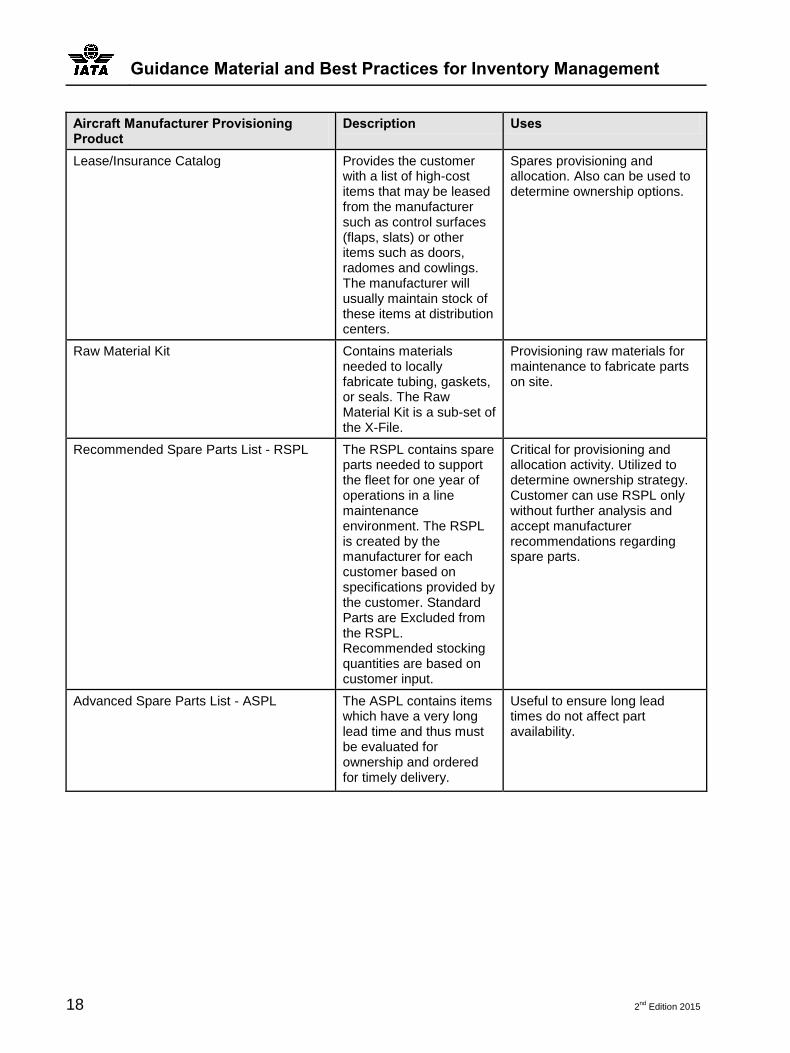
Guidance Material and Best Practices for Inventory Management
18 2nd
Edition 2015
Aircraft Manufacturer Provisioning Product
Description Uses
Lease/Insurance Catalog
Provides the customer with a list of high-cost items that may be leased from the manufacturer such as control surfaces (flaps, slats) or other items such as doors, radomes and cowlings. The manufacturer will usually maintain stock of these items at distribution centers.
Spares provisioning and allocation. Also can be used to determine ownership options.
Raw Material Kit
Contains materials needed to locally fabricate tubing, gaskets, or seals. The Raw Material Kit is a sub-set of the X-File.
Provisioning raw materials for maintenance to fabricate parts on site.
Recommended Spare Parts List - RSPL
The RSPL contains spare parts needed to support the fleet for one year of operations in a line maintenance environment. The RSPL is created by the manufacturer for each customer based on specifications provided by the customer. Standard Parts are Excluded from the RSPL. Recommended stocking quantities are based on customer input.
Critical for provisioning and allocation activity. Utilized to determine ownership strategy. Customer can use RSPL only without further analysis and accept manufacturer recommendations regarding spare parts.
Advanced Spare Parts List - ASPL
The ASPL contains items which have a very long lead time and thus must be evaluated for ownership and ordered for timely delivery.
Useful to ensure long lead times do not affect part availability.

Initial Discussion of Airline Provisioning
2nd
Edition 2015 19
Aircraft Manufacturer Provisioning Product
Description Uses
Peculiar Recommended Spare Parts List - PRSPL
The PRSPL shows parts unique to the new aircraft delivery versus a comparison with those aircraft already in the customer’s fleet; the PRSPL allows the customer to focus on new parts taking advantage of parts they have already provisioned.
An operator of an existing fleet will find this list useful to compare current provisioning with any new provisioning required for the incoming fleet.
Minimum Recommended Spare Parts List
The Minimum Recommended Spare Parts List identifies the minimum spares required to support operations of 1 to 2 aircraft at a customer-designated risk level for approximately 6 months to 1 year. It will typically contain 200 to 300 parts that will see activity in the designated time frame.
A new operator can begin provisioning with this list.
S-File
The S-File is the ATA200/SPEC2000 equivalent of the RSPL. It contains all items in the IPC considered to be potential spares in a line maintenance environment, listing them as LRU.
Used for the same purposes as the RSPL, however data is in ATA200/SPEC2000 format for easy electronic interchange.
Standards Kit
Customized to the aircraft/engine configuration by the manufacturer, the Standards kit contains parts such as fasteners and other maintenance related parts for 3 to 5 aircraft. Quantities are listed in a one-year supply.
Provisioning and Allocating Expendables.

Guidance Material and Best Practices for Inventory Management
20 2nd
Edition 2015
Aircraft Manufacturer Provisioning Product
Description Uses
T-File
The T-File is also ATA200/SPEC20000 based file, customized for the airline showing all items considered to be potential spares (T-File End Items). The T-file contains the information necessary to support the overhaul of the End Items. It is essentially a bill of materials in text format for repair and overhaul parts.
Useful for setting up provisioning for repair and overhaul of components. If a third-party vendor will be overhauling parts for the airline, then the T-File may be extraneous information.
U-File Expands the Bulk Material List to all items called out in any CMM, SRM or AMM such as cements, paints, oils, etc. The Bulk Material Kit is a subset of the U-File. The U-File does not contain recommended quantities for operations.
Useful in a complete maintenance, repair and overhaul environment where the operator will be accomplishing line maintenance, base maintenance, and component maintenance. If third parties provide any phase of maintenance, some or all of the U-File may be extraneous information.
V-File The V-File is an ATA200/SPEC2000 combination of the S-File and T-File. As such it shows all potential spares in a line maintenance and base maintenance environment, including items necessary to support the overhaul of components.
Can be used as a complete listing of potential spares and sub-components required to support overhaul and repair of the spares.
W-File
Contains Special Tools and Test Equipment for aircraft and shop level repair.
The W-File would be used by tooling analysts to assess tooling and test stand needs. If an airline uses third-party maintenance, this may be extraneous information.

Initial Discussion of Airline Provisioning
2nd
Edition 2015 21
Aircraft Manufacturer Provisioning Product
Description Uses
X-File
Identifies raw materials to be stocked in support of local fabrication. It is an expansion of the Raw Material Kit, showing metals and other materials beyond gasket/tubing/seal materials.
Provisioning raw materials for maintenance to fabricate parts on site.
Y-File
Lists all pool candidate items worldwide. The manufacturer provides the airlines using the same part numbers as the fleet the customer has purchased.
Can be used to determine ownership. Can be useful in contacting partners for pooling and borrow strategies.
Z-File
The Z-File contains items required for maintenance of the tools and test equipment located in the W-file.
The Z-File would be used by tooling analysts to assess tooling and test stand maintenance needs. If an airline uses third-party maintenance, this may be extraneous information.
On-Board Flight Kit or Fly Away Kit (FAK) Contains recommendations for items to be carried with the aircraft into remote locations. Parts in the FAK will have already been recommended in the RSPL.
Useful for charter, cargo or military operations into remote, difficult to serve locations where part failure would result in extended downtime for the aircraft.
ETOPS Significant Parts List
Reference only for parts critical to ETOPS (Extended-range Twin-engine Operational Performance Standards) flight status.
Highlights ETOPS critical parts already contained in the RSPL.
Maintenance List
Provides items necessary during scheduled maintenance checks for the aircraft.
General provisioning for airframe maintenance (base or line maintenance).
Master Minimum Equipment Parts List (MMEL)
The MMEL is a subset of the RPSL and references RSPL items to MMEL categories.
Spares provisioning and allocation. Also can be used to determine ownership options. Can be used to limit ownership/allocation to only flight critical items.
Table 2. Aircraft Manufacturer Provisioning Products

Guidance Material and Best Practices for Inventory Management
22 2nd
Edition 2015
The most critical manufacturer-provided data files for spares planning include the G-File, Lease/Insurance
catalogue, RSPL, S-File, and the Y-file. If the operator has ETOPS aircraft, then the ETOPS Significant
Parts List is critical. If the operator will be involved in overhaul of parts as well, then the T-file will be
necessary. However, if the operator will engage a third party for repair and overhaul of components, then
the T-File can be deemed extraneous information unless it will need to be provided to the operator’s
vendors.
3.1.2 Operational Data from another Carrier with the Same or Similar Fleet
Often other operators have experience with the fleet in question. It can be useful to have operator data in
addition to the products offered by the aircraft manufacturer. If an airline has close relations with another
operator, perhaps a data sharing and interchange will be useful in making fleet sparing evaluations. Keep in
mind that the MTBR and contained in the RPSL and other manufacturer-provided documents are often
different than those experienced in actual operations. Consider that a higher than published MTBR/MTBUR
will reduce spares requirements and a lower than published MTBR/MTBUR will result in higher spares
requirements. Also highly variable MTBR/MTBUR will impact spares decisions. In addition, manufacturers
are often held to the published MTBR/MTBUR as a guaranty and if an operator experiences worse
performance than expected, commercial remediation in the form of no-cost spares lease and potentially
other benefits are due to the airline. In addition, once the reliability issue is corrected and MTBR/MTBUR
increases to its design level, the excess spares an airline may own will now be surplus.
Note that due to competitive issues, an airline operating the same fleet may not freely offer this type of
information and data for use by a new or emerging carrier. If this is so, some other options may be explored
such as third-party maintenance providers or industry consultants.
3.1.3 Data from an MRO Partnering with the Carrier for Spares
Provisioning and Repair/Overhaul
In addition to potentially partnering with another airline to share data, a third-party MRO vendor may also be
able to provide the airline with operational data. In fact, MRO data may be a blended version of several
airlines MTBR/MTBUR and thus give a better estimate for the airline in evaluating spares requirements.
Since many MRO and other third-party maintenance providers partner with airlines to provide inventory
support, often a good cooperation can be set-up between the airline planning functions and the MRO
planners since both have a vested interest in fleet performance and spares performance.
3.1.4 Data from Industry Experts or Consultants
A fourth source of data would be from industry experts or consultants working in the field of aviation material
management. Like an MRO or third-party maintenance provider, consultant data may represent a cross-
section of the industry and therefore more closely approximate MTBR and MTBUR under operational

Initial Discussion of Airline Provisioning
2nd Edition 2015 23
conditions. If a carrier does not plan to utilize an MRO or third-party maintenance provider, and cannot
secure cooperation with a competing airline, an industry consultant may be able to provide the best source of operational data available to a start-up operator or an operator expanding with a new fleet type.
3.2 How to Provision for Airline Operations
If an inventory manager chooses the G-file and RSPL can be accepted at face value from the manufacturer
and used to stock main bases and stations with spares. If this method is used, most of the topics and techniques discussed in this guideline are unnecessary, however, keep in mind that this approach may lead to a very large balance of slow moving inventory. It is recommended to use the aircraft manufacturer
provisioning products, but to always make a determination based on the techniques outlined in this book whether to own and allocate inventory.
An alternative approach is used in this guideline. The inventory manager should not discount the
manufacturer provided data, however, one should investigate options for providing the lowest total cost and the highest possible service. The remainder of this guideline is dedicated to methods for achieving high
service levels at low cost.
If an airline is starting up operations, the inventory manager must decide upon ownership options. If a
manager is inheriting continuing operations, then an inventory balance likely exists. Regardless of inventory balance, the equations to allocate stations are the same. Ownership can be evaluated during the Nine Step model below.
3.2.1 Nine Step Model to Determine Rotable Inventory Support for Airline Operations
The process of provisioning Rotables for airline operations can be summarized in the Nine Steps listed
below:
1. Understand Airline Operational Goals
2. Gather Needed Data
3. Calculate Annual Demand
4. Designate Parts as Stock Items
5. Calculate Station Qualification
6. Determine Allocation Quantities and Locations
7. Determine WIP Support Inventory Levels
8. Formulate Procurement Strategy
9. Monitor and Improve Inventory System
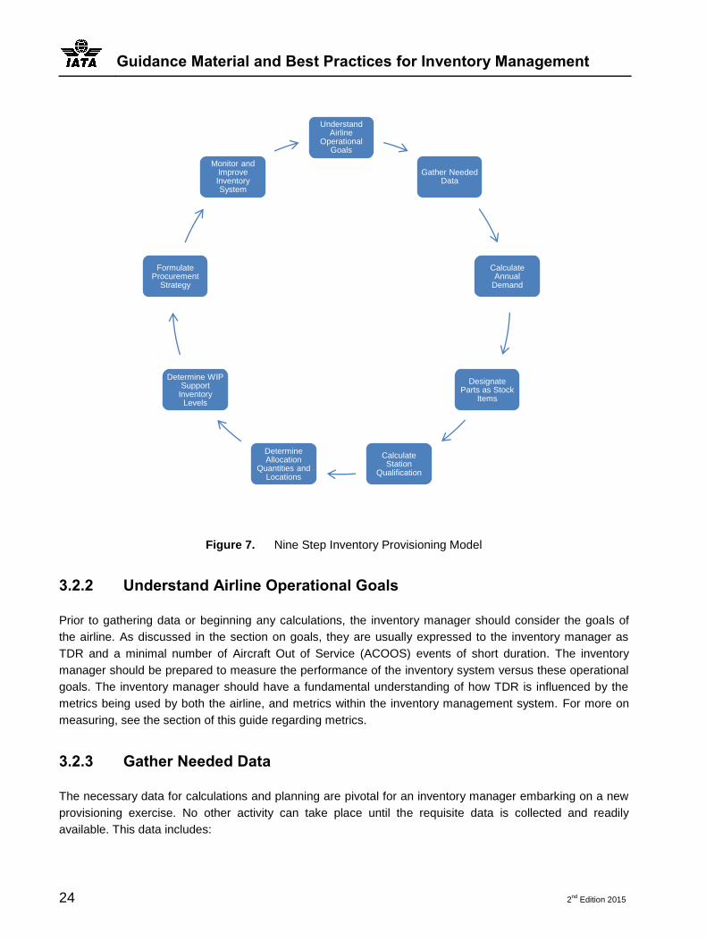
Guidance Material and Best Practices for Inventory Management
24 2nd
Edition 2015
Figure 7. Nine Step Inventory Provisioning Model
3.2.2 Understand Airline Operational Goals
Prior to gathering data or beginning any calculations, the inventory manager should consider the goals of
the airline. As discussed in the section on goals, they are usually expressed to the inventory manager as
TDR and a minimal number of Aircraft Out of Service (ACOOS) events of short duration. The inventory
manager should be prepared to measure the performance of the inventory system versus these operational
goals. The inventory manager should have a fundamental understanding of how TDR is influenced by the
metrics being used by both the airline, and metrics within the inventory management system. For more on
measuring, see the section of this guide regarding metrics.
3.2.3 Gather Needed Data
The necessary data for calculations and planning are pivotal for an inventory manager embarking on a new
provisioning exercise. No other activity can take place until the requisite data is collected and readily
available. This data includes:
Understand Airline
Operational Goals
Gather Needed Data
Calculate Annual
Demand
Designate Parts as Stock
Items
Calculate Station
Qualification
Determine Allocation
Quantities and Locations
Determine WIP Support
Inventory Levels
Formulate Procurement
Strategy
Monitor and Improve Inventory System
Initial Discussion of Airline Provisioning
2nd
Edition 2015 25
Fleet types to be operated.
RSPL for each fleet type showing:
o MPN for each part effective on the operator’s aircraft.
o OEM MTBR.
o QPERAC – number of each part effective on the operator’s aircraft.
Operational data including:
o Daily planned utilization in hours and cycles.
o Station specific flight schedules showing equipment, flights per day (including any day-to-day
differences in flight schedule), and flying hours into each station, by equipment type.
Expected TAT for repair of each part, expressed in days.
Scrap percentages for each part.
Replenishment lead times for each part.
For an inventory manager faced with allocating and provisioning in an existing inventory system (i.e.
operations have been ongoing prior to the current allocation cycle), most of the data above is readily
available by virtue of the prudent inventory manager’s data collection and measurement system. Typically
the only changes to this type of system come from changes in Operational Data (flight schedule, new
service in new stations, changes in aircraft utilization etc.). To the extent possible, an inventory manager
should try to get a pre-briefing on any significant changes from the previous period’s operations to assess
the impact to the inventory management system. If any one or combinations of the following factors are not
homogenous with prior period data, expect that the inventory management system and allocations should
undergo evaluation for change:
Increase/Decrease in aircraft utilization (hours or cycles).
Addition/Deletion of service.
Opening/Closing maintenance stations.
Increase/Decrease of fleet size.
Addition of new fleets (this will become an initial provisioning exercise).
Current or planned aircraft modifications which may require upgraded components.
o Note should be taken that if the airline has done modifications in the prior year(s) that the data in
regards to removal or consumption will be skewed and the inventory manager needs to factor that
in. Example if the airline has upgraded its In-Flight Entertainment (IFE) system the data will show
substantial higher amount of removals for the old IFE system components the years the modification
took place.
Changes in sourcing strategy for part repair which may affect planned component repair TAT.
Flight schedule changes which result in concentration or dispersal of fleet types across their historic
range.

Guidance Material and Best Practices for Inventory Management
26 2nd
Edition 2015
International destinations that may have specific issues such as customs that will impact shipments or
storage of parts. In some instances, use of a FAK may be required to offset the issues of part
availability. International destinations may also have an increased allocation over and above a
comparable domestic station to offset part availability issues.
Any of the above bulleted points can drive significant costs to the airline due to changes in sparing
requirements. In order to have as much advance warning of significant operational changes in the airline, it
is highly recommended that the inventory manager participate in the airline planning process as much as
possible. For example, a planned aircraft modification desired by the airline’s Marketing Department may
drive extensive procurement costs due to sparing requirements; if the inventory manager is actively
participating in the airline planning process, then this information can be used in evaluating the initial
decision. If the inventory manager does not participate in the airline planning process the manager should
request that all information regarding any operational changes are distributed in order for the manager to
react accordingly and in a timely manner.
3.2.4 Calculate Annual Demand
When calculating the annual demand we need to gather at least the following:
Fleet type(s) to be operated
RSPL for each fleet type showing:
o MPN for each part effective on the operator’s aircraft
o OEM MTBR
o QPERAC – number of each part effective on the operator’s aircraft
Operational data
o Daily planned utilization in hours and cycles
Expected repair TAT in days for each part
o The TAT must be realistic in the way that it should display the days from when a serviceable part
leaves the stores until a part is available again in the stores area.
The inventory manager can calculate annual demand on a part number by part number basis. For
continuation of operations, the new planned annual demand should be checked versus prior year’s demand
for any significant changes, and these part numbers can be flagged for further analysis and decision
making.
Note that demand may increase or decrease for a variety of reasons. The inventory manager should be
cognizant and conversant in all the possible causes, but recognition of the planned increase or decrease is
paramount. An increase in demand could drive additional procurement activity or otherwise cause a
degradation of service (assuming the inventory balance was right-sized to previous activity levels). A
decrease in demand could be temporary, but if the decrease is permanent, then there is the potential for

Initial Discussion of Airline Provisioning
2nd
Edition 2015 27
surplus activity. Often, the inventory manager should have a horizon that matches the operational budgeting
horizon since planned purchase and surplus activity should be estimated in the budget planning process.
For an initial provisioning exercise, the annual demand should be estimated at the earliest possible time.
The following elements will drive some degree of initial provisioning:
Addition of a new fleet type to an existing fleet of aircraft (e.g. Adding B767-300ER to a fleet of all B757
and A320 aircraft).
Addition of new aircraft within an existing fleet type (e.g. Adding 20 B737-800 to the existing fleet of 54
aircraft for a total of 74 aircraft).
Beginning operations in their entirety (first year of airline operation).
Opening of a new maintenance base or station designed to have significant maintenance activity.
Growth of prior service by a significant amount (e.g. Airline XYZ previously flew 1 flight per day to
London-Gatwick and in the new schedule has a daily frequency of 20 flights per day).
Addition of new service (e.g. beginning multiple daily frequencies to several destinations in the same
region).
After calculating annual demand for every part, this data should be saved in a spreadsheet or other format
for use in later steps.
3.2.5 Designate Stock Items
After calculating demand for every individual part number, generally in a spreadsheet format, the next step
would be to sort the MPNs. The MPNs would needed be sorted into, but not limited to, the following
category. First is to view those listed as No-Go. The next is to sort them by MEL category. And finally the
complete listed should be sorted by estimated annual demand. When viewing MPN by MEL category, care
must be taken to consider that certain faults impose operational restrictions even though the aircraft is
released to service. With the highest demand at the top, and the lowest demand (including zero demand
and those very miniscule quantities), the inventory manager should delineate the demand into several
categories, based on projected annual removal volume:
Very High Demand Parts
o Examples include batteries, wheels, tires, brakes, etc.
o Very high demand can be driven by low MTBR, a large quantity of parts installed on the operator’s
aircraft, a very large fleet, high frequencies, or a combination of these factors.
Parts with demand > 1 per year
o Often these parts make economical candidates for ownership and we will explore that in owned vs
leased assets later.

Guidance Material and Best Practices for Inventory Management
28 2nd
Edition 2015
o Many different MPN’s will be in the category of demand >= 1 removal per year. The actual number
of MPNs with annual demand >= 1 will vary according to fleet types, however expect between 150-
300 parts per aircraft type.
o While lower in volume than the Very High Demand Parts, any part that has at least one removal per
year should garner significant attention from the inventory manager.
o While an ownership or leasing model is economical if removals are greater than one per year, there
may be pooling or exchange arrangements that can be more financially competitive than
ownership/leasing, we will explore that in owned vs leased assets.
Parts with annual demand < 1.0
o Since we will show later that removals can be assumed to follow a Poisson Process1, an annual
demand of approximately 0.50 removals per year can also be read to assume that there will be one
removal every two years on average.
o Organizational memory may prevent the inventory manager from effectively discounting removals
that are only occurring on a semi-annual basis.
o Further, the inventory manager may find that if all the parts with demand <1.0 are summed for an
annual period, a significant number of unfilled part requests and resultant operational impacts could
occur.
o No-Go and Go-If parts should be given special consideration due to their impact to flight operations.
o Parts that can be placed on Deferred Maintenance list or MCO and the aircraft dispatched with the
part inoperative can be dealt with on an economic basis.
Parts with demand much less than one per year
o If demand is non-existent, these parts should be designated as Not A Stock Item (NASI) until such
time as their removal activity increases the demand to move the part into a higher volume category.
3.2.6 Calculate Station Qualification
Determining station qualification is the process of taking aggregate demand for the inventory system and
determining how the removals will be distributed to the various stations the airline serves. Many airlines refer
to the station qualification process interchangeably with the allocation process. The term station qualification
refers to the act of determining if the removal activity driven by flight hours will qualify the station for an
allocation of each part number in question. The equations and calculations will be covered in detail in
Understanding Provisioning Calculations. The calculations are essentially the same as for the system level
demand discussed above, but are calculated at the station level.
1 (Boeing, Commercial Airplane Group, Customer Services Division 1997)
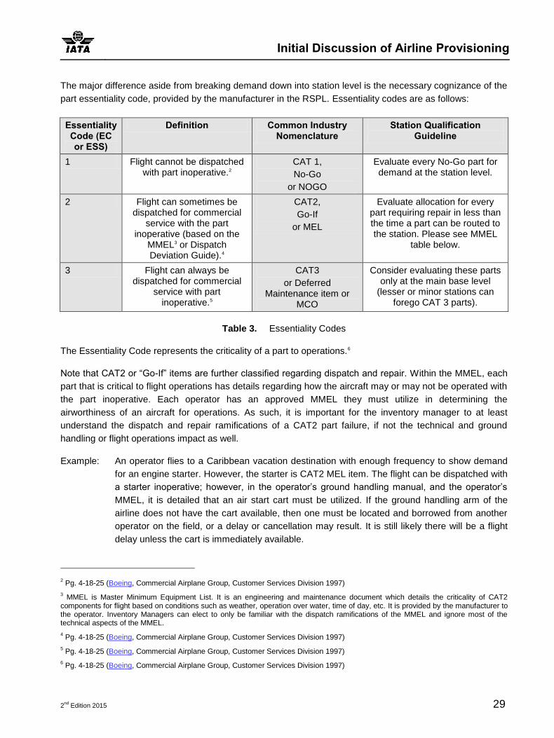
Initial Discussion of Airline Provisioning
2nd
Edition 2015 29
The major difference aside from breaking demand down into station level is the necessary cognizance of the
part essentiality code, provided by the manufacturer in the RSPL. Essentiality codes are as follows:
Essentiality Code (EC or ESS)
Definition Common Industry Nomenclature
Station Qualification Guideline
1 Flight cannot be dispatched with part inoperative.2
CAT 1,
No-Go
or NOGO
Evaluate every No-Go part for demand at the station level.
2 Flight can sometimes be dispatched for commercial
service with the part inoperative (based on the
MMEL3 or Dispatch Deviation Guide).4
CAT2,
Go-If
or MEL
Evaluate allocation for every part requiring repair in less than the time a part can be routed to the station. Please see MMEL
table below.
3 Flight can always be dispatched for commercial
service with part inoperative.5
CAT3
or Deferred Maintenance item or
MCO
Consider evaluating these parts only at the main base level
(lesser or minor stations can forego CAT 3 parts).
Table 3. Essentiality Codes
The Essentiality Code represents the criticality of a part to operations.6
Note that CAT2 or “Go-If” items are further classified regarding dispatch and repair. Within the MMEL, each
part that is critical to flight operations has details regarding how the aircraft may or may not be operated with
the part inoperative. Each operator has an approved MMEL they must utilize in determining the
airworthiness of an aircraft for operations. As such, it is important for the inventory manager to at least
understand the dispatch and repair ramifications of a CAT2 part failure, if not the technical and ground
handling or flight operations impact as well.
Example: An operator flies to a Caribbean vacation destination with enough frequency to show demand
for an engine starter. However, the starter is CAT2 MEL item. The flight can be dispatched with
a starter inoperative; however, in the operator’s ground handling manual, and the operator’s
MMEL, it is detailed that an air start cart must be utilized. If the ground handling arm of the
airline does not have the cart available, then one must be located and borrowed from another
operator on the field, or a delay or cancellation may result. It is still likely there will be a flight
delay unless the cart is immediately available.
2 Pg. 4-18-25 (Boeing, Commercial Airplane Group, Customer Services Division 1997)
3 MMEL is Master Minimum Equipment List. It is an engineering and maintenance document which details the criticality of CAT2
components for flight based on conditions such as weather, operation over water, time of day, etc. It is provided by the manufacturer to the operator. Inventory Managers can elect to only be familiar with the dispatch ramifications of the MMEL and ignore most of the technical aspects of the MMEL.
4 Pg. 4-18-25 (Boeing, Commercial Airplane Group, Customer Services Division 1997)
5 Pg. 4-18-25 (Boeing, Commercial Airplane Group, Customer Services Division 1997)
6 Pg. 4-18-25 (Boeing, Commercial Airplane Group, Customer Services Division 1997)

Guidance Material and Best Practices for Inventory Management
30 2nd
Edition 2015
The above example highlights why MEL items are very critical to operations and significant attention should
be given during the evaluation for allocation. The categories of MEL are as follows:
CATEGORY A
Items in this category shall be repaired within the time of interval specified in the “Remarks or Exceptions”
column of the operator’s approved MEL. Whenever the provision in the “Remarks or Exceptions” column of
the MMEL states cycles or flight time, the time interval begins with the next flight. Whenever the time interval
is listed as flight days, the time interval begins on the flight day following the day of discovery
CATEGORY B
Items in this category shall be repaired within 3 consecutive calendar days excluding the day of discovery.
CATEGORY C
Items in this category shall be repaired within 10 consecutive calendar days, excluding the day of discovery.
CATEGORY D
Items in this category shall be repaired within 120 consecutive calendar days, excluding the day of
discovery. To be considered for placement in Category D, the item must be of an optional nature, or excess
equipment which an operator may, at his/her discretion, deactivate, remove from or install on an aircraft.
Note that all of the MEL items A through D have the potential to restrict operations. Note also the main
differential between A, B, C and D items are the timeframe in which a failed part must be replaced or
repaired. Many operators treat MEL A the same as No-Go when evaluating for allocation.
All of the MEL items have the potential to restrict operations, however, when allocating, the inventory
manager can use the MEL to advantage if the conditions requiring the part to be operative do not exist in the
network or at the station being allocated. An example would include parts that restrict operations over water,
however the operator does not have flights over water. Similar situations may exist regarding night
operations, operations of restricted visibility, icy conditions, etc. Further, MEL items are prime candidates for
pooling or borrowing contingencies, if another operator routinely carries the part in question on the field. An
inventory manager can save the cost of part ownership/leasing by covering a borderline allocation with a
part that can be made available by one or more pooling or borrow partners on the field. More on pooling will
be discussed later.
The steps for determining station qualification are outlined below. The pivotal data element needed at this
juncture is the detailed flight schedule showing daily frequencies and flight hours into a station. Of course, if
annual demand above has been calculated, then all the relevant part number data is available (the RSPL,
MPN, MTBR, QPERAC, total number of A/C).
At this stage, many airlines with large networks will utilize computer software to assist in the allocation
process. However, a moderate sized operation could accomplish the allocation process with a spreadsheet.

Initial Discussion of Airline Provisioning
2nd
Edition 2015 31
Keep in mind in progressing through the inventory allocation process, decisions are being made at the
individual part number level. There are numerous ways to accomplish allocation, ranging from least to
greatest in complexity and greatest to least in part investment:
Allocation Methodology Complexity Level Expected Investment
OEM Recommendation via RSPL Low Medium to High
Calculation by Individual part number Moderate Medium-high to Medium-low
Optimization (usually accomplished with computer software)
High Medium to Low
Table 4. Contrasting Allocation Methodologies
OEM recommendations via the RSPL generally come in tiers. These tiers are structured according the age
of the aircraft, and to an extent are customized by the OEM for the specific operator to which the fleet is
delivered. The RSPL recommendation and tier system is necessary and useful when a fleet is brand new,
with little historical data.
A second option arises when there is significant operator data available for the fleet(s) in question. Whether
the inventory manager has a large database and long history with an existing fleet operated by the home
airline, or the data is provided by a another operator who also operates the fleet, MTBR data is based on
actual operations and can make a significant impact on the investment level required. At this juncture in fleet
life, often less investment will be realized if actual historical MTBR from an operator can be used in
calculations.
A third option arises due to the availability and power of computational resources. Complex optimization
algorithms can be run literally overnight, applying criteria to data sets to provide the highest possible service
level at the lowest total cost. The output of any optimization model should be cross-checked with experience
and perhaps some old fashioned hand (or spreadsheet) calculations, but in general if the inventory system
is adequately modelled, excellent optimization results can be expected. Complexity is increased with this
option because significant groundwork is required and data integrity is paramount, otherwise optimization
model results may be skewed.
The basic steps for station allocation are as follows:
1. Obtain RSPL
2. Familiarize with Essentiality and MMEL categories of each part
3. Obtain station specific flight schedule
a. Should show, by fleet type, flights and hours/cycles into each station
b. Planned aircraft maintenance overnight activity should also be considered
4. At the station level, sum the total flight hours on an annualized basis for each fleet type serving each
station
5. Order stations by summed flight hours from greatest to least
Guidance Material and Best Practices for Inventory Management
32 2nd
Edition 2015
a. Often within a schedule there are multiple stations with similar hours/cycles totals. If this is the case,
one station can be evaluated for allocations and the resulting analysis applied to the remaining
similar stations.
6. Evaluate the station with the greatest number of flight hours for every part that is designated as a stock
item (you may ignore NASI parts at this time)
a. For every fleet into the station create a matrix of MPNs based on the RSPL and QPERAC for each
fleet type.
b. Create a matrix for each fleet type.
7. Evaluate the station with the next greatest number of flight hours similar to the first station (6) above.
8. Continue until every station has been evaluated or the level of flight activity at the stations does not
qualify the remainder of the ordered list for allocation.
There are some important considerations for allocation models:
Multi-Effective Parts: These are parts which can be utilized on a number of different fleets. A single-fleet
operator can ignore the impact of multi-effectivity. However, an operator with multiple fleet types must
cross-reference each part to make sure all flight hours are accounted for against that part. For example,
there are numerous B757 and B767 parts which are cross-effective on both fleets. In addition, some of
these same parts are cross-effective on B737NG as well. In determining if a station qualifies for
allocation of a specific MPN that is cross effective on all three fleets (B757, B767, B737NG), then the
inventory manager must sum all flight hours by these 3 fleets into the station, multiplied by each
effective QPERAC
o Example: MPN BA24180R1, Halon Fire Extinguisher Bottle, is effective on multiple fleets.
Previously a station received only B757 service, and the QPERAC is 4 bottles. However due to
schedule change, B767-300 and B737-800 service is added to the station. For B767-300 the
QPERAC is 4 bottles and for the B737-800, QPERAC is 2 bottles. Assume that each aircraft type
flies 1000 hours annually into the station. The sum of total hours accounting for all three fleets would
be: 1000 X 4 (B757) + 1000 X 4 (B767-300) + 1000 X 2 (B737-800) = 10,000 Hours.
o Suppose that in the above example, the 1000 hours of B757 service was replaced with 1000 hours
of additional B737-800 service, and B767-300 service remained at the same level in the next
schedule change. In this example, the QPERAC and multi-effectivity becomes even more important
since the B737-800 QPERAC is half of the B757 (2 per a/c versus the B757 4 per a/c). In this case
the sum of total hours would be: 2000 X 2 (B737-800) + 1000 X 4 (B767-300) = 6000 hours. This
example illustrates clearly how important QPERAC and multi-effectivity can be.
Regardless of actual station allocation calculations and the qualification process, it will be rare to have a
station with zero allocations. Often an airline will create a minimum station allocation that is automatic
with the inception of service at the station. Expect that the high demand parts identified in the Calculate

Initial Discussion of Airline Provisioning
2nd
Edition 2015 33
Annual Demand step will be candidates for the minimum station allocation list. Examples are
wheels/tires, brakes, batteries, oxygen bottles7, etc.
Related to minimum station allocations are FAK. FAKs are generally utilized by operators who have zero
tolerance for Out of Service (OOS) due to parts, examples being military, cargo, and charter operations.
Often operators who desire a FAK have irregular schedules versus regularly scheduled commercial
service into predictable destinations. Coupled with irregular schedules may be a moderate to large
degree of uncertainty regarding future destinations
o Note that provisioning and transporting a FAK on every aircraft can be quite expensive (duplication
of inventory with low utilization, increased fuel costs, reduction in passenger and freight load).
o A FAK may be practical when future destinations are unknown and/or have a low degree of logistics
options into or out of the destination. Examples are charter, freighter and military charter operations
into remote or otherwise inaccessible regions of the world. If a FAK is called for, then it should be
verified that a mechanic will be readily available to perform maintenance.
o FAK provisioning should be balanced with actual station allocation and logistical options for moving
parts into expected operating regions and calculations made that ensure the risk to operations
justifies the total cost of FAK usage.
Another important consideration for an inventory manager when running allocations analysis is the
availability of different options in the stations being evaluated
o For example, a carrier beginning brand new service to New York City via JFK should evaluate the
options already on the field in terms of pooling and borrow opportunities before automatically
allocating parts to JFK merely by virtue of the start of new service.
o Often there are several dominant carriers already serving the same station who may be willing to
provide an inventory pool.
o In addition to operators, MRO providers, various surplus providers and/or OEM may have pooling
options in place in popular destinations, or be willing to enter into a form of partnership if
approached regarding pooling options.
3.2.7 Determine Allocation Quantities and Location
The previous step, Determine Station Qualification, is intended to mathematically determine every station
that should be allocated. However, in practical application, the inventory manager will take the allocation
calculations and balance them with several other factors and make a decision whether to truly allocate the
station with an actual physical asset owned or leased by the airline or provide for the need through another
method such as borrow or pooling.
7 If the operator has good planning on maintenance events, batteries and oxygen bottles would not be required. On the other hand it is
good practice to check services available before making decisions on those items.

Guidance Material and Best Practices for Inventory Management
34 2nd
Edition 2015
The chart below fundamentally illustrates the thought process. The triggering event is always part failure,
either anticipated due to demand calculations, or an actual event.
Figure 8. Situations with Potential for Inventory Consolidation
Factors that may influence a manager to decide NOT to allocate an otherwise qualified station include
the following:Parts that are CAT3, Deferred Maintenance parts or MCO
o Parts that allow the aircraft to be dispatched with the part on Deferred Maintenance list or MCO are
prime candidates for consolidation at a few locations within the airline network.
o Once the Deferred Maintenance or MCO is applied, the flight can be dispatched and plans can be
made to change the part either:
At a location where both the part and labor is available to perform the maintenance.
At a location where the aircraft operates and the part can be shipped to on short notice.
Deferred Maintenance
Part
•Consolidate Deferred Maintenance parts in a few locations
•Route to overnight or thru flight maintenance stations if necessary
Long Removal Step
• Elapsed Time of Removal Step will allow for routing part into failure station
• Confirm List of candidate parts with Line Maintnenace and MCC
MEL
• If failed part will not immediately restrict operations, route part to aircraft or aircraft to part
• Confirm with Maintenance all MEL decisions
• Aggregate calcualted demand for the part at the regional level when allocating to another station
Special Tooling
• Special Tooling examples include jacks and jack stands that may need to be shipped from another location
• Parts that require special tooling for removal such aircraft jacking (eg. landing gear retract actuator) should be allocated in the same locations as the tooling required for their removal
Part Failure

Initial Discussion of Airline Provisioning
2nd
Edition 2015 35
The required part may either already be allocated to the planned repair station or the part may
be routed to the location where maintenance will prefer to change the part with minimal flight
impact.
o Network analysis can be used to determine the most logical stations for concentration of CAT3
components
Most airline networks will have one to several stations that are good candidates for inventory
consolidation.
Candidate stations will have a high frequency of daily flights and therefore many logistic options
for moving parts into and out of the station, as well as facilitating movement of an aircraft
requiring repair into the station with the consolidated inventory.
Parts that have an extended removal step
o If a part can be routed to a failure location, even if it is No-Go or Go-If, before the removal can be
accomplished, then an inventory manager would be wise to minimize allocations.
o Aircraft engines are prime examples. Some engine types have a removal step with a long-enough
elapsed time that the engine can be shipped and delivered to the aircraft without impacting the
critical path of the engine replacement.
o Other examples include:
APU
Windshields for the most part depending on location and frequency of service or total recovery
time
Fuel control units
Some generators
Stabilizer trim motors or drives
Thrust reversers
Flight control panels including flap and slat segments or spoilers
o It is recommended to partner with maintenance to determine a list of candidates for consolidation
due to elapsed time.
MEL Parts that will not affect operation between city pairs
o For example, if an MEL part fails, but the restriction is over-water operations and all city pairs from
the failure station are over land, then it is not necessary to allocate an MEL part with over-water
restrictions to the station in question.
o Since the demand will qualify the station for allocation, the MEL part should be allocated
somewhere, but preferably where it is of most use to maintenance. In this way, aggregate all
demand for the part and allocate regionally.
o Confirm the list of consolidation candidates with maintenance and operations.
Parts that require special tooling
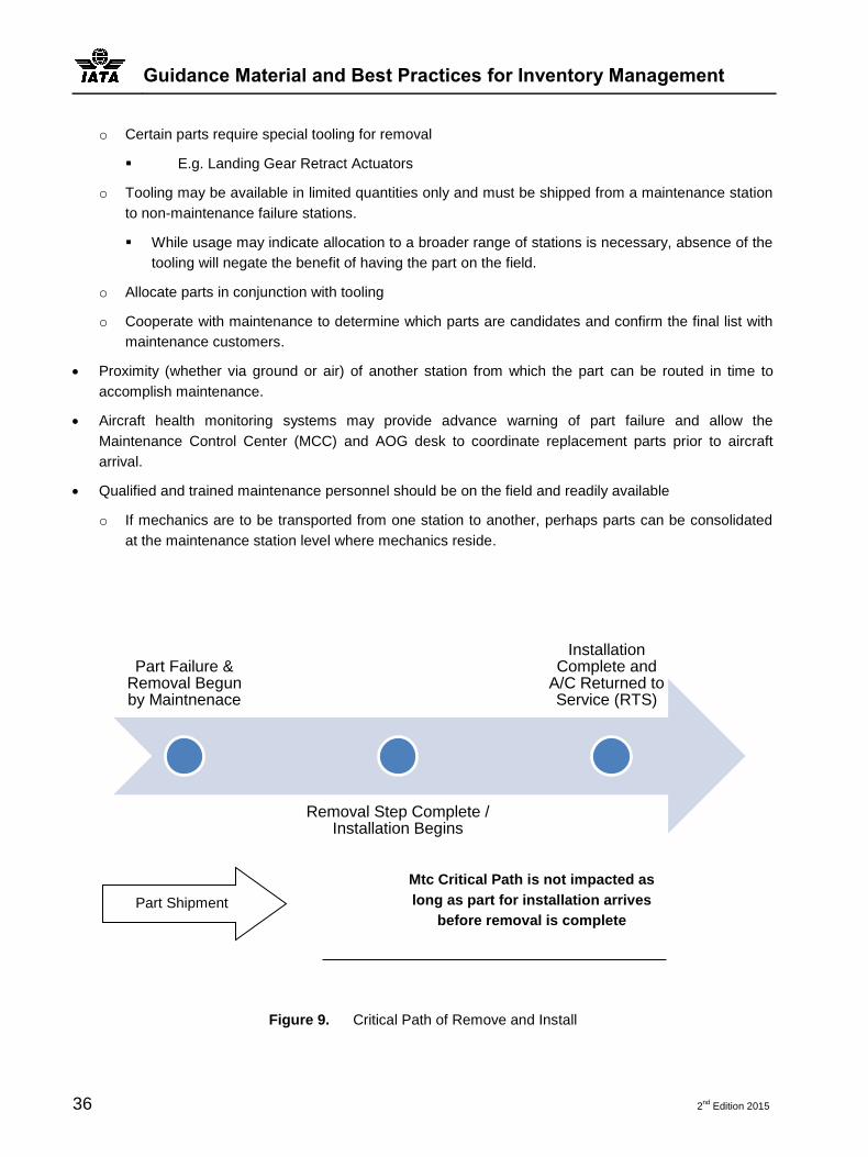
Guidance Material and Best Practices for Inventory Management
36 2nd
Edition 2015
o Certain parts require special tooling for removal
E.g. Landing Gear Retract Actuators
o Tooling may be available in limited quantities only and must be shipped from a maintenance station
to non-maintenance failure stations.
While usage may indicate allocation to a broader range of stations is necessary, absence of the
tooling will negate the benefit of having the part on the field.
o Allocate parts in conjunction with tooling
o Cooperate with maintenance to determine which parts are candidates and confirm the final list with
maintenance customers.
Proximity (whether via ground or air) of another station from which the part can be routed in time to
accomplish maintenance.
Aircraft health monitoring systems may provide advance warning of part failure and allow the
Maintenance Control Center (MCC) and AOG desk to coordinate replacement parts prior to aircraft
arrival.
Qualified and trained maintenance personnel should be on the field and readily available
o If mechanics are to be transported from one station to another, perhaps parts can be consolidated
at the maintenance station level where mechanics reside.
Figure 9. Critical Path of Remove and Install
Part Failure & Removal Begun by Maintnenace
Removal Step Complete / Installation Begins
Installation Complete and
A/C Returned to Service (RTS)
Mtc Critical Path is not impacted as
long as part for installation arrives
before removal is complete
Part Shipment

Initial Discussion of Airline Provisioning
2nd
Edition 2015 37
It is strongly urged that for every category of part under consideration, the inventory manager should involve
the maintenance constituency to garner their experience and support.
The outcome of this step should be a reduction in inventory ownership. For example, if a number of stations
qualify for an allocation based on annual demand in each station of one removal per year for the part, and
flights can be operated with the failed part inoperative, consolidation is limited only by the supply chain that
replenishes allocated stations.
Example: If a part is calculated to have an aggregate annual demand of 24 distributed among 6 stations
according to the following table:
Station Annual Demand Maintenance Station
A 5 Yes
B 4 Yes
C 3 No
D 3 Yes
E 5 No
F 4 No
TOTAL 24 3 Maintenance Stations
Table 5. Fictional Part Demand for 6 Stations
Also consider that the part is a CAT3 Deferred Maintenance part or MCO. Shipment time (in hours) between
stations is shown in the matrix below (assumes shipment from all city pairs is possible):
Station / Station
A B C D E F
A NA 5 3 4 3 2
B 5 NA 4 4 3 3
C 3 4 NA 3 2 4
D 4 4 3 NA 2 3
E 3 3 2 2 NA 2
F 2 3 4 3 2 NA
Table 6. Matrix of Trans-shipment times in hours between stations
Even though stations E and F have comparable removals to the maintenance stations A and B, we might
only allocate one of the maintenance stations. Consider that annual aggregate demand is 24. This means
that on average, there is one removal every 15.2 days. If the repair pipeline is robust enough to return parts

Guidance Material and Best Practices for Inventory Management
38 2nd
Edition 2015
with confidence in less time that the average removal time, then a part allocation of just one unit can be
justified.
A WIP level would be required to allocate only 1 station8. For example, if repair TAT is 30 days, then
WIP level can be calculated as following:
o Where dd is daily demand or annual removals divided by total days per year.
o In this case:
o TAT as stated is 30 days, so WIP calculation is as follows:
One might argue it would be better to take all 3 units and allocate them to the 3 maintenance stations,
however, due to the demand level, WIP is calculated as 2 units. If we make the conscious decision to
allocate all 3 units owned, we will perpetually run 2 backorders for this part in the inventory system once
the system reaches steady state.
If the one allocated part can be expeditiously moved by the AOG desk, then the most economical
solution for our example would be to own or lease three units, allocate one and utilize the other two for
WIP support9.
If TAT was half of 30 days at 15 days, WIP level would be reduced by half from 2 to 1 unit.
Using probability, risk can be calculated by using the Poisson Distribution, according to the probability
formula10
( )
The symbol represents the rate of occurrence. In our example the annual rate is 24 removals per year.
In calculating risk, we are concerned that the number of removals would exceed the total number of
serviceable units in the system at any given time.
Consider the system representation below
8 WIP levels will be discussed in another section.
9 For more on WIP support please see the next section of this guidebook, “Determine WIP Support Inventory Levels”
10 (Kiemele, et al. 1999)

Initial Discussion of Airline Provisioning
2nd
Edition 2015 39
Figure 10. Representation of the Removal and Repair Cycle Showing the Repair Pipeline
Consider that Airline Operations generate failures of components for which replacements are drawn
from Station Inventory.
At removal, the unserviceable unit enters into the state of WIP inventory, or WIP “pipeline”, often
referred to as merely pipeline inventory. It is the inventory which sustains the repair process.
We might ask the question: What is the chance that we have removals between the time of a removal
using the last serviceable spare and the replenishment of the next serviceable unit from the Repair
Station?
To determine this we’ll use the equation above, and sum the probability of occurrence:
( ) ∑
o Situation: Station Inventory is empty, having just been consumed and creating a backorder. We
should calculate the probability that a removal occurs in the time frame of our repair process.11
11 Note that for this example we assume that repair is a discrete 30 days, and is not an average, nor an average rate of arrival. In other
words, repair takes exactly 30 days, no more, and no less. We assume this because many repair contracts and arrangements guarantee a TAT of a certain interval as a NTE or Not To Exceed number-in our case, 30 days.
WIP or Pipeline
Station inventory
Repair Station
Airline operation
Flow of Repairs in
days <= TAT
Flow of Removals at rate
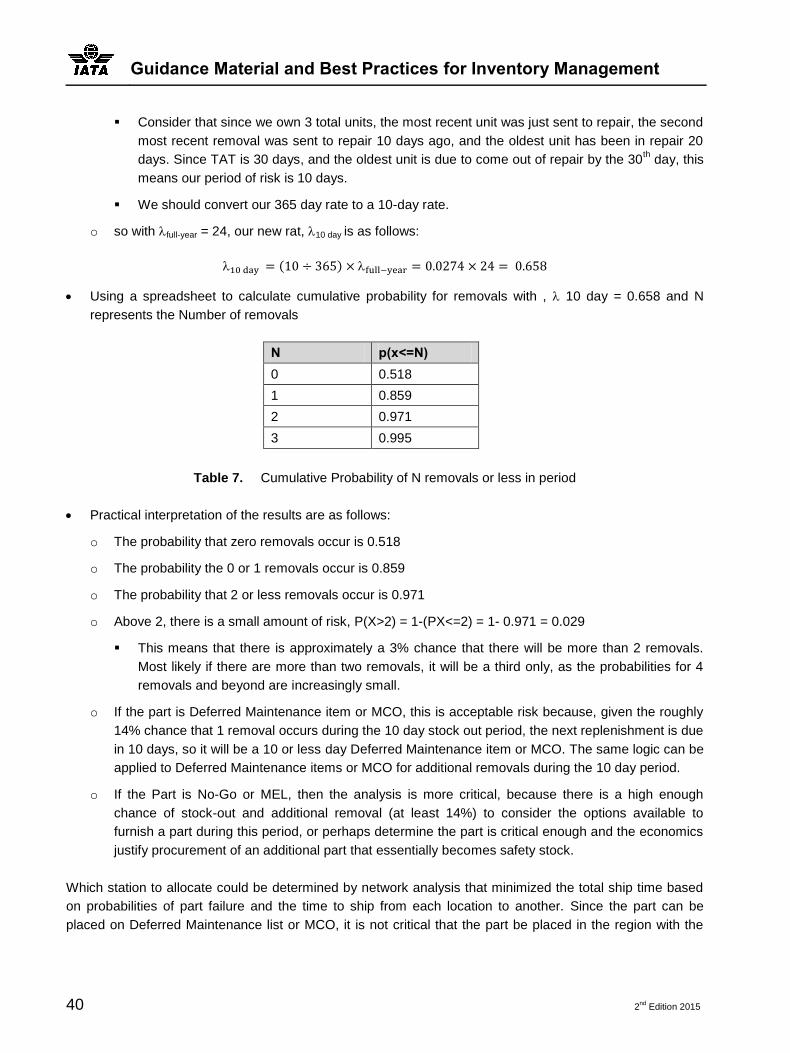
Guidance Material and Best Practices for Inventory Management
40 2nd
Edition 2015
Consider that since we own 3 total units, the most recent unit was just sent to repair, the second
most recent removal was sent to repair 10 days ago, and the oldest unit has been in repair 20
days. Since TAT is 30 days, and the oldest unit is due to come out of repair by the 30th day, this
means our period of risk is 10 days.
We should convert our 365 day rate to a 10-day rate.
o so with full-year = 24, our new rat, 10 day is as follows:
( )
Using a spreadsheet to calculate cumulative probability for removals with , 10 day = 0.658 and N
represents the Number of removals
N p(x<=N)
0 0.518
1 0.859
2 0.971
3 0.995
Table 7. Cumulative Probability of N removals or less in period
Practical interpretation of the results are as follows:
o The probability that zero removals occur is 0.518
o The probability the 0 or 1 removals occur is 0.859
o The probability that 2 or less removals occur is 0.971
o Above 2, there is a small amount of risk, P(X>2) = 1-(PX<=2) = 1- 0.971 = 0.029
This means that there is approximately a 3% chance that there will be more than 2 removals.
Most likely if there are more than two removals, it will be a third only, as the probabilities for 4
removals and beyond are increasingly small.
o If the part is Deferred Maintenance item or MCO, this is acceptable risk because, given the roughly
14% chance that 1 removal occurs during the 10 day stock out period, the next replenishment is due
in 10 days, so it will be a 10 or less day Deferred Maintenance item or MCO. The same logic can be
applied to Deferred Maintenance items or MCO for additional removals during the 10 day period.
o If the Part is No-Go or MEL, then the analysis is more critical, because there is a high enough
chance of stock-out and additional removal (at least 14%) to consider the options available to
furnish a part during this period, or perhaps determine the part is critical enough and the economics
justify procurement of an additional part that essentially becomes safety stock.
Which station to allocate could be determined by network analysis that minimized the total ship time based
on probabilities of part failure and the time to ship from each location to another. Since the part can be
placed on Deferred Maintenance list or MCO, it is not critical that the part be placed in the region with the

Initial Discussion of Airline Provisioning
2nd
Edition 2015 41
most failures, what is most critical is that the part can be placed in a location that minimizes total ship time,
since shipment will burn fuel, a precious and expensive commodity in today’s market.
Through optimization (network analysis and mathematical programming)12, the lowest total cost solution can
be found that:
Minimizes Inventory Investment
Maximizes Aircraft Service Level
Minimizes Transshipment costs (fuel burn & transactional costs)
Often an inventory manager may operate under guidelines that dictate if removals are above a certain level
(e.g. 4 times per year) then allocate a part. In the above example there are 4 stations with removals greater
than or equal to 4 per year. This would result in 4 units being allocated across the example system.
3.2.8 Determine WIP Support Inventory Levels
As we found in the example concluding the last section, “Determine Allocation Quantities and Location”, the
WIP inventory and station inventory are intertwined and related via TAT. Also, the desire to manage
backorders properly would drive an inventory manager to adequately partition inventory between station
inventory and WIP inventory. In essence, total inventory is a combination of WIP inventory level and station
inventory levels or:
∑
Some airlines are able to dispense with either WIP or station inventory ownership via pooling or leasing
arrangements, or arrangements with a comprehensive MRO provider that also provides full inventory
support. However, someone must still calculate the needs of the airline based on flight activity and generate
the resultant demand that is compared with TAT to ensure that enough inventory is held to provide for the
desired service level.
WIP inventory arises in support of the repair process that is inevitable with Rotable spares. In Expendable
management, WIP inventory is synonymous with safety stock used to cover RLT.
Recent trends in airline inventory management point to creating partnerships between MRO providers and
the airlines. Often, in conjunction with a maintenance agreement, airlines will join an inventory pool provided
by the MRO partner. One obvious benefit to the airline is the elimination of carrying costs associated with
WIP.
12 For discussions regarding network analysis and other related topics, please see (Winston 1991)

Guidance Material and Best Practices for Inventory Management
42 2nd
Edition 2015
In this step of the inventory model, aggregate annual demand once again comes into play. At the highest
level, all removals will in effect flow through the same repair station, regardless of whether repair is
accomplished internal or external to the airline. As such, the level of WIP to support the repair pipeline
should be aggregated as well.
WIP support or pipeline inventory must be calculated for each individual MPN.
For each part number, calculate WIP according to the following formula:
Where dd is daily demand or annual removals divided by total days per year:
WIP calculations will often result in fractional numbers. WIP Results such as 2.97, 3.42 and 1.05 will be
commonplace. However, inventory provisioning is done at the integer level; an airline either owns or leases
1 or 2 or 3 or more of each MPN.
It is not recommended to simply round up or round down each calculation. One of the nice features of the
WIP calculation is that the decimal element of the calculation can be utilized to roughly estimate the number
of days in the year that a stock-out (backorder) will occur during the course of the year if the inventory
manager elects to always round down on the WIP calculation.
Example:
Using the aforementioned 24 removals per year and 30 day TAT, we calculated WIP level to be 1.97
units.
As a result of the WIP calculation, plus the analysis done prior showing the wisdom of a single allocated
unit (since the part is Deferred Maintenance item or MCO), the inventory manager previously decided to
own a total of 3 units, 1 for allocation and 2 for WIP support.
Suppose that in the new year, demand is forecasted to increase to 28 units per year due to addition of
leased aircraft to the fleet and increase in aircraft utilization overall.13
The new WIP calculation would be as follows:
13 For treatment of demand calculations in this guidebook, please see the section 6, “Understanding provisioning calculations”.

Initial Discussion of Airline Provisioning
2nd
Edition 2015 43
If the inventory manager is under pressure to keep inventory levels constant, and elects to keep WIP
and station spares at a total of 3 units, note that 30% of the year (the 0.30 of 2.30) the station spare will
be utilized as WIP pipeline support inventory.
In other words, the station spare will be utilized and a backorder will persist until the 1st unit inducted at
the repair station returns to station inventory, and backorders will be carried for 109.5 days in the station
inventory.
o This could translate into risk as follows:
Convert annual demand of 28 into 109.5 days of demand as follows:
( )
Assume the Poisson distribution with = 8.4, what is P(X=0), probability that there are no removals in
the 109+ days of station backorder?
Using a spreadsheet to calculate, we find the Poisson Probability P(X=0) with = 8.4 is 0.000225
The probability that there are more than zero removals can be represented as follows:
( ) ∑ ( )
So
( ) ∑ ( )
This gives the result:
( ) ( )
This result can be interpreted practically that it is almost a certainty that there will be a removal in the
aggregate 109.5 days of backorder during a 365 days of operation.
Another nice feature of the Poisson distribution is that the rate can be used to estimate the mean, or
expected number of occurrences in an interval. For the Poisson, this is expressed as follows:
( )
For our example, this means the number of removals with no replenishment can be expected to be 8.4
annually (the value of during our calculated 109.5 days of carrying backorders).
o In practical application, this will become 8-9 purchases, borrows, exchanges or other method of
procurement for No-Go parts and 8 or 9 Deferred Maintenance items or MCO for an aggregate
average of 109.5 days, or each on Deferred Maintenance list or MCO for an average of 12.2 days to
13.7 days.
o With the exchange rate on the surplus market at 10% of Fair Market Value (FMV) it might be wise
for an inventory manager to consider those in order to cover those periods when nil stock. And if

Guidance Material and Best Practices for Inventory Management
44 2nd
Edition 2015
exchanged unit is only placed on stock and never used it can be returned, in many cases, with only
added a restocking fee.
o If the inventory manager is forced to go with loan or borrow to cover the nil stock periods those can
quickly add up. Even if the inventory manager’s airline was stellar at borrow removal, and costs only
tallied 10% CLP per event (this would generally be the access fee of 8%, plus only 2 days of borrow
time at 1% CLP per day)14 then the 8-9 events would still total 80%-90% CLP, in which case surplus
items may still be available at much less than this annual cost.
o Of course when determining to purchase a part rather than borrow and pay-as-you-go, the impact of
capital spending versus operational expense is raised. Evaluating this example purely as cash flow,
it is clear that procuring the WIP part versus borrowing it constantly is the preferred decision with the
more positive impact to cash flow. However, if a part is purchased, there are additional annual costs
and if the procure vs. borrow is not clear cut, then an Net Present Value (NPV) analysis would be in
order to ensure the manager takes the right decision.
In summary, WIP levels are important and it is critical to properly account for the impact of changes in
demand on the pipeline (WIP) inventory. If WIP levels are not properly maintained, an escalating series of
backorders, Rotable service level erosion, stock outs, and ultimately service level impacts will result
(Deferred Maintenance or MCO, and potential DL/CX due to No-Go part availability). During every schedule
cycle, the inventory manager should recalculate and evaluate WIP level for each part with changing
demand.
3.3 Formulate Procurement Strategy
This step refers to the process of determining how the inventory manager will provide for the calculated
inventory needs highlighted in the previous two sections discussing station allocation and WIP inventory.
Assuming that annual demand has already been calculated and inventory needs have been identified,
whether the assets are destined for station support (allocated) or pipeline support (WIP), the inventory
manager should now turn to the most economical solution for acquiring physical assets to meet the needs of
the operation. There are multiple options open to the inventory manager for procurement and provision of
assets:
Ownership
Leasing
Pooling arrangements with other carriers, OEMs, MROs, or dedicated companies
Borrow
Exchange
Rob
14 For more detailed treatment of loan/borrow in this guide, please see Borrow Strategies

Initial Discussion of Airline Provisioning
2nd
Edition 2015 45
3.3.1 Ownership
Many airlines default straight to ownership if there is a defined need for an asset. In fact, many operators
who have had continuing fleet operations for a number of years have built a substantial balance of owned
inventory. Occasionally, there are parts on the operators books that at one time were in great demand,
however, have fallen into disuse. However, usually the majority of the inventory in an airline’s possession
has some activity level.
The advantages of ownership include:
Possession of the inventory negates fears regarding the future state of asset levels.
o For example a lessor or cooperating partner cannot recall the inventory, or move the inventory to
another location.
o Lessors or other partners may have a desire to sell the inventory as surplus while the asset value is
still high.
The owner is free to make decisions on scrap replacement.
o If a part is scrapped in the course of maintenance and the inventory manager can forecast declining
demand for the part, the manager can choose not to bear the cost of scrap replacement.
o Also the inventory manager can decided to replace only when the need comes up.
Possession of inventory as the owner allows the inventory manager to place the inventory wherever he
chooses.
o Lessors may place restrictions on regions where their asset can be placed due to risk factors.
o Pooling partners generally place inventory with their primary location and the pool participants have
little influence in the location.
Often the airline will view ownership of assets as an investment, with a residual value that can be used
to generate cash at a later date.
There are disadvantage to ownership as well:
Generally airlines do not realize a competitive residual value on surplus assets
o Surplus assets generally arise en masse at the announcement of fleet retirement.
o Once the market is aware that operator plans to reduce or retire a fleet, buyers will offer lower
purchase prices based on the impending flood of parts on the market.
o Further, consider that if an airline is one of two major operators of a unique or aging fleet, then if the
other operator announces retirement first, the market will become depressed and the airline will be
unable to take any action which can mitigate this risk.
Ownership generally results in a very high carrying cost that the airline must bear year over year.
o The total carrying cost may approach or even exceed 20% per year in depreciation, taxes,
insurance, obsolescence, and cost of capital.

Guidance Material and Best Practices for Inventory Management
46 2nd
Edition 2015
Some of the expense is real cash cost, negatively impacting cash flow.
Depreciation is realized on the income statement.
There can be a situation where a firm can have a positive free cash flow, but report a net loss due to
depreciation expense.
o When determining whether to purchase or pursue another method of procurement, NPV analysis
should be used to evaluate purchase versus the other available options.
o Airlines can assume too high a residual value on the inventory.
Ensure that an accurate residual or salvage value is utilized in financial calculations such as
NPV.
Ownership of inventory assets ties up capital that could be used in other areas.
If a firm must borrow to purchase, the cost of borrowing should also figure into the total cost of
ownership.
3.3.2 Leasing
Leasing is often a natural second selection, particularly when the inventory assets may be tied to a short-
term fleet plan. Examples include:
The fleet being supported by the inventory is on a fixed short-term lease.
It is known the fleet has an impending reduction or retirement within the next 8-10 years.
Other common reasons for leasing include:
Aircraft modification or AD-related activity that requires enhanced part support for an extended period of
time, but not long enough to justify ownership.
Damage or repair to a large structure or surface
o OEM’s and brokers generally offer leasing on expensive components that are not economical for
individual airlines to own.
o MRO providers may offer short-term leasing in conjunction with accomplishing repair or modification
to a fleet for the airline.
However, consider that leasing can be very competitive on a year over year basis with purchase. The
primary reason for this is the differential in cost of capital for an airline versus the usually lower cost of
capital for a lease provider.

Initial Discussion of Airline Provisioning
2nd
Edition 2015 47
Ownership Leasing
Cash Non Cash Cash Non Cash
Lease Expense NA 28%
Taxes and Insurance 6% NA15
Cost of Capital 15%16
Loan Cost 8%
Depreciation 8%17
Obsolescence18 NA NA
Total Cash Cost 29%
Total Expense19
(Cash + Non Cash Cost)
37%
28%
Table 8. Comparison of Ownership Cost versus Leasing
Leasing is often dismissed as not cost effective and negatively affecting cash flow. However, even if the
cash is available to the firm and the parameters of the example above change so that the loan expense is
non-existent, the firm must still “invest” the purchase price of the part, for which it may do well to expect a
20% return (salvage value) as a single payment in the future. In addition, the lease rate of 28% is assumed
to be high for the sake of example. Often the airline may be able to negotiate lower lease rates.
3.3.3 Owned Versus Leased Assets
Once it has been determined that certain part numbers will require full time access for station allocation or to
support repair with WIP, the inventory manager must decide whether to purchase or lease the required
assets. Often, the default decision is purchase. Purchase is ideal if there are abundant assets on surplus
market, affording a discount versus CLP. Purchasing assets is also often selected if the fleet plan calls for
the effective aircraft to be in service with the operator for many years. Purchase is often required when
faced with inventory that has high scrap rates, since the inventory will be replaced many times over the life
of the parent aircraft.
Leasing assets does not always appear as a logical choice to operators, however there are a number of
scenarios where leasing assets can be very attractive. First, if there is a short term need due to aircraft
modification or perhaps damage repair, leasing surfaces, flight controls or components is often the lowest
15 Tax and Insurance is assumed to be paid by owner of record and is included in the lease rate
16 Often referred to as hurdle rate of IRR (internal rate of return). It is the assumption that if the cash is available, it can be invested in
some other venture other than that under consideration and the investment will yield an annual return.
17 Assumes a straight line depreciation model, with 10 year duration, 20% salvage value
18 Obsolescence is scrap replacement, loss, damage, theft etc. will be the same regardless of whether the part is purchased or leased.
If lost/damaged or deemed scrap, the part will be replaced at FMV (fair market value).
19 Expense to the firm’s Income Statement

Guidance Material and Best Practices for Inventory Management
48 2nd
Edition 2015
cost option. Purchase in this situation is often ill-advised since once the part is no longer needed by the
airline, the part must either be placed in surplus sales or held in inventory for an indefinite period, collecting
the expense of carrying cost for many years to come.
Leasing assets is also very attractive if the aircraft fleet plan either has a very short horizon or aircraft
retirement is imminent. In cases where it is known that the effective life of an aircraft fleet type with the
airline is less than 10 years, lease of required assets can be a very attractive option financially and
operationally. In fact, leasing often has a distinct advantage over purchase due to the issue of salvage value
or residual value of an asset.
Salvage value or residual value is critical to any lease versus purchase decision. Consider that in calculating
the NPV for a purchase, one must consider the eventual re-sale of the asset and how much money will be
recovered at that time. Many times the actual salvage value is modelled too high in the analysis. Reality for
airlines is that they are fortunate to recover 20% of the residual value, unless the fleet is in high demand.
Year 1 2 3 4 5 6 7 Total
Initial balance $ 80,000 $ 71,429 $ 62,857 $ 54,286 $ 45,714 $ 37,143 $ 28,571
Cash Investment $ (80,000)
T&I $ (4,800) $ (4,286) $ (3,771) $ (3,257) $ (2,743) $ (2,229) $ (1,714)
Cost of Capital $ (12,000) $(12,000) $(12,000) $(12,000) $(12,000) $(12,000) $(12,000)
Surplus sale
$ 20,000
Cash Totals $ (96,800) $(16,286) $(15,771) $(15,257) $(14,743) $(14,229) $ 6,286 $(166,800.00)
Purchase NPV $(156,843)
Cash Flow $ (22,400) $(22,400) $(22,400) $(22,400) $(22,400) $(22,400) $(22,400) $(156,800.00)
Lease NPV $(139,558)
Table 9. Cash Flows for Purchase versus Lease
Cost of capital is 15%
T&I is 6%
Lease rate is 28%
o The lease rate is always a commercial issue and can be either higher or lower.
CLP is assumed $100,000 and resale price 20% of that.
Purchase price and leasing was assumed $80,000.
In this example we see that the leasing option has less negative NPV then purchasing.

Initial Discussion of Airline Provisioning
2nd
Edition 2015 49
Also, in the example it is assumed the firm has adequate free cash flow to purchase the part without
borrowing. If borrowing cash is required the NPV analysis is even more favorable to leasing versus
purchase.
Cost of Capital is assumed to be the opportunity cost for using the money to buy parts versus some
other venture.
Consider that International Airline Technical Pooling (IATP) leasing can be found at 18% of acquisition
value, then leasing is an even more attractive option versus purchase when it is known that the fleet will
retire or exit the airline in less than a decade.
Note that short term leases carry higher lease rates. OEM typically offers leasing of critical large parts such
as flight controls for 1/365th of CLP per day. With leasing partners, generally leases in the 5-7 year range are
practical. When leasing for 3 years or less expect high annual rates, sometimes approaching 30% per year.
Lease rates can be variable and are as critical to NPV analysis as any other factor. IATP leasing assumes
an IATP partner either has the item in a warehouse or is willing to acquire the part prior to leasing.
Other factors to consider include the scrap rate of the leased part. However, one can argue that a
component with a high scrap rate can still be favourably leased. The scrap rate of the part is independent of
the method of acquisition, whether it is purchase or leased. Most lease terms between supplier and
customer stipulate that at the conclusion of the lease, a like part must be returned, recognizing that the
same serial number may not be available after years of service. In addition, this clause contained in most
lease contracts eliminate the need for special routing aircraft to remove parts that may have been installed
and need to be returned at lease end.
Leasing is a similar solution to Pooling and Inventory Exchange. Often the analysis is the same, but
contractually the terms may be different and the nomenclature of the part provisioning may change. The
major difference with a lease between a supplier and a customer is that the customer retains full control of
the asset for the life of the lease. In pooling and exchange solutions, often the supplier controls the assets
and as such there may be service level risks, as many airlines are drawing on the same pool of inventory.
Outright leasing affords the same service level protection as purchasing inventory as a financially attractive
option.
The above discussion has assumed also that the lease is an operating lease. The primary distinction for a
capital lease is that at the end of the lease, the lessee becomes the owner of record and title passes from
the supplier to the customer. By definition, an operating lease is an expense, contrasted with a capital lease
which may have tax implications. To differentiate between an operating lease and a capital lease, there are
a series of accounting tests that must be used to classify the lease as either operating or capital. The
inventory manager is encouraged to consult with their accounting or finance department for a clarification on
any leases being considered.

Guidance Material and Best Practices for Inventory Management
50 2nd
Edition 2015
3.4 Options other than Ownership or Leasing
Full-time control of assets via outright ownership or leasing can be very attractive for certain types of
operations and levels of station qualification. These options include inventory pooling, borrowing of parts
from other operators, exchanges with other operators or inventory providers, and robbing one’s own fleet.
The first decision an inventory manager should make is whether the station is a good candidate for a
strategy other than ownership or leasing. If activity levels are high in a station, then the operator will likely
require ownership or long-term leasing. If, for example, the operator has 100 flights daily transiting a station,
that station is likely not a candidate for a non-ownership pool or borrow option because the operator is likely
at least one of the major airlines in that station. However, the operator could take its leased or owned
inventory and aggregate demand from other operators with less activity in the station to offset the cost of
purchase or lease to provision the station.
On the other end of the spectrum is a station with 1 flight daily (or less frequency). The operator may be able
to find a willing partner that already has adequate and appropriate inventory stationed on the field.
In practical application, most stations an operator considers are going to be between the two extremes of
major station and single daily frequency.
3.4.1 Inventory Pooling
Pooling with another operator, a commercially available pool, or entering into a new partnership with an
inventory vendor in a pool will require some pre-planning. Someone must determine activity level in the
station, either at the individual airline level, or aggregating several sets of airline flight hours into the station.
Next, one or several firms must be convinced to place the inventory in the station, or the operator must
search for a willing partner desiring to enter into a new market. Pooling arrangements afford many types of
business structures, from simple sharing of like-sized inventory balances up to joint-ventures where perhaps
one partner provides the investment in inventory whereas the other handles the logistics.
There are several options in pre-determined pools available. One such pool is the IATP,
http://www.iatp.com/. Fundamentally, the IATP offers a pooling forum for airlines to cooperate, reduce the
cost of inventory, increase service level, and provides some ground rules and structure to the pools
sponsored by members. One particularly nice feature is visibility to member airlines’ inventory. This visibility
can help an inventory manager decide whether to stock a station or participate in a part offered by a co-
operator.
A commercially available on-line application which allows members to view each other’s station inventory is
AeroExchange (https://www.aeroxchange.com/). AeroExchange and similar product offering are not only
useful in the planning stages, but also for the airline’s AOG desk in sourcing components when a failure
occurs during live flight operations or overnight maintenance activity. While AeroExchange is not a pool per
se, but is a visibility tool, it does provide functionality necessary for successful inventory pooling.

Initial Discussion of Airline Provisioning
2nd
Edition 2015 51
Payment for pooling can come in various forms. Biannually payments that net an airline’s provided parts
with shared parts is common with IATP type pooling and is accomplished via IATA Clearing House. If an
airline provides (supplies) more parts to the pool than they share (utilize), then the airline will receive a net
revenue check. If the airline uses more parts than it provides, then a payment will be due to the
clearinghouse from the airline. In general, in this type of pooling, it is desired that the airline share versus
provide is balanced overall. In other words, airlines that only use assets from the pool are encouraged to
contribute value, often at another station location. Some airlines provide more parts then they use and will
receive a net revenue check every month. It is uncommon for an airline to be able to utilize the pool unless
they are also a provider.
Vendor and partner generally structure pool payments as monthly payments, either flat rates, Power By the
Hour (PBH) or included with repair cost. Fundamentally, from a payment perspective, this type of pool is not
different from a lease. However, a pool sometimes may be entered and left freely, has no guarantee of
availability, and the pool provider may elect to move the asset the airline is interested in, transferring parts
from one station to another as a result of a schedule change or some other reason. Pools will often have
many users/participants, and the airline should assess the risk at each location that a part will be available
when needed. Pool availability and sharing is contrasted with leases which are generally 100% dedicated to
the lessee.
3.4.2 Borrow Strategies
Purposely creating a borrow strategy for parts is wise if the volume of the parts in question is less than one
removal a year. If a pooling strategy as described above is utilized, the airline should expect to pay a
guaranteed expense, independent of volume or usage. In essence, pooling is billed to the airline as an
access fee-if there is no usage, the airline will still pay for the access. When compared to pooling, borrowing
is a pay-as-you-go arrangement, and is volume sensitive, as well as time sensitive.
The amount an airline will pay depends on both the number of borrow events as well as the duration of each
event. Typical charges per borrow include an 8% set-up fee, as well as per day charges that escalate as the
duration grows. All fees are based as a percentage of CLP, and if a borrow lasts a number of days in
duration, significant charges can be incurred. The set-up fee is incurred if the borrowing airline agrees to
take the part on loan, and is independent of whether the part is actually installed on the customer aircraft.
Typical Loan Borrow Fees can be as follows:
Borrow/Loan Charges
% of CLP
Borrow/Loan Charges
% of CLP
Borrow/Loan Charges % of CLP
Access fee 8% Access fee 8% Access fee 8%
Daily fee day 1-10 1% Daily fee day 1-14 1% Daily fee day 1-10 1%
Daily fee day 11-20 1.50% Daily fee day 15-30 2% Daily fee day 11-30 2%
Daily fee day 21+ 2% Daily fee day 31+ 3% Daily fee day 31+ 3%
Table 10. Customary Loan Fees for Aircraft Parts20
20 These three are only examples, other variations are possible

Guidance Material and Best Practices for Inventory Management
52 2nd
Edition 2015
Borrow/Loan charges when aircrafts become AOG are very quick to add up to high amounts. If these
charges are not monitored closely, preferably on daily basis, it can cause financial setback to the inventory
manager goals and the airlines as well. The following table shows how the cost of a loan or borrow is versus
exchange. Market exchange is normally done on 10% access fee based on FMV and the charges to return
the Unserviceable (US) component to Serviceable (SE) condition. Normally the airline will receive from 21
up to 30 days to return an US component back to the vendor. This is different between vendors and is often
left up to commercial negotiation. Note that it is often not possible to obtain an exchange to cover an AOG
and in most cases when a component can be found at the station of the AOG, usually with another operator,
that option is obviously the first option in order to minimize the delay or risk of cancellation of flight. Also it
shows if you mix the two in order to minimize the cost. The following calculation is based on the borrow/loan
rates in column 6 above and the exchange cost is 10% of FMV.
Component A B C D
CLP $ 30,000 $ 50,000 $ 75,000 $ 150,000
FMV $ 15,000 $ 25,000 $ 45,000 $ 85,000
EXCH COST $ 1,500 $ 2,500 $ 4,500 $ 8,500
2 day loan $ 3,000 $ 5,000 $ 7,500 $ 15,000
5 day loan $ 3,900 $ 6,500 $ 9,750 $ 19,500
10 day loan $ 5,400 $ 9,000 $ 13,500 $ 27,000
15 day loan $ 8,400 $ 14,000 $ 21,000 $ 42,000
25 day loan $ 14,400 $ 24,000 $ 36,000 $ 72,000
35 day loan $ 21,900 $ 36,500 $ 54,750 $ 109,500
Ex+2 day loan $ 4,500 $ 7,500 $12,000 $ 23,500
Ex+5 day loan $ 5,400 $ 9,000 $14,250 $ 28,000
Table 11. Borrow/loan vs exchange calculation
The following should be mentioned that we leave out the repair charges for the component that failed due to
the reason that the cost for that will always occur, if the airline uses its own inventory, borrows or does an
exchange that cost will be the same.
Another option regarding exchanges is a flat exchange fee. What that means is that the airline will only pay
this onetime fee for the access of the component and no repair/overhaul charges will occur. Airlines that
have substantial data on component repair/overhaul cost should be able to quickly determine if that fee is
fair. It can also be a good option as it gives the airline certainty on the total cost for the component failure.
Borrowing can be a good option when an inventory manager examines annual demand for AOG parts and
notices that there are hundreds of parts that have annual demand less than one per year, and many of them
very fractional demand that will translate to one removal every several years. Justifying purchasing of parts
that will be utilized once every few years will be difficult at best. Also, considering that the purchase must be
repeated for every qualifying station in the carrier’s network and a very stagnant inventory balance of
millions of dollars can be built up. These types of parts with fractional annual demand are great candidates

Initial Discussion of Airline Provisioning
2nd
Edition 2015 53
for both pooling and borrow, with those on the lower end of the demand spectrum being the most likely and
economical candidates for borrow.
A wise inventory manager would investigate borrow opportunities prior to determining what borrow strategy
is the best to cover the operation. It will be difficult to borrow a part not located at the station in question, so
finding a willing borrow partner is much like searching for pooling partners. In fact, they may often be one
and the same and may invite the inventory manager’s airline to join a pre-existing pool for the parts in
question. At this time a manager should perhaps take a probabilistic approach to the money spent to cover
the operation. If removals are more of a certainty, then pooling will be more economical than borrowing. For
the list of parts in question, a blend between pooling, borrow, exchange, and outright ownership or leasing
will be adopted for each station.
To do a probabilistic analysis, a comparison of how many borrow events, an inventory manager will need to
evaluate annual demand, the cost to pool, the borrow duration, the borrow cost per event, and calculate the
total annual borrow cost expected. Then the inventory manager can select the lowest cost option, part by
part, assuming a pooling or loan provider is available at the station in question. To facilitate analysis, an
inventory manager might create the following table:
MPN Expected annual number of removals
21
CLP22
Pooling Cost
23
Borrow Duration
24
Borrow Cost/ Event
25
Total annual Borrow Cost
26
Recommendation27
123 0.5 $100,000 18% 10 18% 9% Borrow
234 0.15 $85,000 9% 10 18% 3% Borrow
345 0.25 $25,000 6% 30 53% 13% Borrow
456 0.3 $15,000 9% 8 16% 5% Borrow
567 0.75 $5,000 18% 18 34% 26% Pool28
Table 12. Comparison of Pooling versus Borrow strategy
21 E(X) = t because we assume a Poisson Process. Remember to express and t in equivalent units. For example, if is expressed in
removals per year, then using t=1 is appropriate. If is a daily rate, then t=365.
22 Note that the decision to pool or borrow is independent of CLP. CLP is included if the manager wishes to calculate an annual
expected cost for the blended pool/borrow solution.
23 Pool cost differences are set by provider. Often IATP is 18% of CLP. If more than one airline shares in the pool, the cost is shared
among the airlines. If 2 share, then annual cost is 9% to each, if 3 share annual cost will be 6% to each, and so on
24 Driven by repair time-may be different for various MPNs. This potential difference is reflected in the example.
25 Borrow Cost Per Event calculated using Borrow Duration and data contained above, column 2.
26 Expected number of removals X Borrow Cost Per Event
27 Recommendation is evaluated by the cheapest annual cost of pooling versus Total Annual Borrow Cost
28 Since Pooling is generally not charged to the user on a per event basis, but rather as an access fee, pooling expense is volume
independent. Borrows are volume dependent. In this case the annual removal rate of 0.75 per year coupled with the fairly long expected time to remove the borrowed part, pooling is the best option in this case.

Guidance Material and Best Practices for Inventory Management
54 2nd
Edition 2015
Note that if borrow is selected, generally the loaning airline requires a credit check and agreement to the
carrier’s loan contract in advance. If borrow is to be pursued as a strategy in a station, it would be wise to
complete General Terms Agreement (GTA) prior to start of service since a borrow can be required any time.
One other interesting facet of borrowing a part is that if the part is returned and requires maintenance, the
borrower is responsible for the charges incurred to repair or overhaul the part and the loan charges can still
apply until the part returns from maintenance. This may seem strange but it has been standard industry
practice for a number of years and this is also in the IATP guidelines for borrow return.
An inventory manager should be well aware of the regulations in his state. For instance the EASA regulation
allow for a temporary installation of a component without it having the required documents29.
3.4.3 Exchange
Exchange has been briefly touched in the borrow section above. Exchange is a mechanism whereby a
serviceable unit is forwarded to the requesting airline in promise for an unserviceable core. Exchanges can
take place between airlines or between a vendor and an airline. Exchanges are often used as result of
maintenance visits, aircraft ground damage or FOD, or when it is desirable to only remove the failed or
damaged part once (i.e. fuel tank entry, special tooling required, long install/remove steps, etc.).
Evaluating exchanges for inclusion in a sourcing strategy can be accomplished in the same way as Table 12
Comparison of Pooling versus Borrow strategy above.
Exchanges are often built into MRO agreements, whereby the airline procures maintenance and an
exchange is included in the pricing or available a la carte. Often exchanges and pooling with an MRO or
other partner are interchangeable terms.
As mentioned above the exchanges usually come in two options, exchange + repair or flat exchange.
Expect to pay perhaps 10% of FMV per event plus repair to the core. If it is found that a part is frequently
exchanged, the part should be evaluated for purchase, lease or pooling. Exchanges should only be used on
very infrequently removed parts. If the exchange is only to cover an unusual removal rate or frequency of
removals with shorter interval then expected the airline should consider returning a serviceable unit. This is
not always an option but it should be explored especially if the airline has its own inventory, has what it
considers favourable repair/overhaul agreements for the component. If the vendor is willing to accept a
serviceable unit to close out the exchange it can save the airline money on the repair charges. In addition to
managing the repair/overhaul themselves the airline might benefit also if the MRO has a rebate program.
29 EASA 145.A.50 Certification of Maintenance (f)
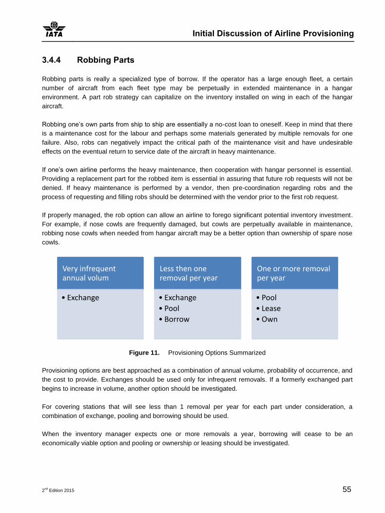
Initial Discussion of Airline Provisioning
2nd
Edition 2015 55
3.4.4 Robbing Parts
Robbing parts is really a specialized type of borrow. If the operator has a large enough fleet, a certain
number of aircraft from each fleet type may be perpetually in extended maintenance in a hangar
environment. A part rob strategy can capitalize on the inventory installed on wing in each of the hangar
aircraft.
Robbing one’s own parts from ship to ship are essentially a no-cost loan to oneself. Keep in mind that there
is a maintenance cost for the labour and perhaps some materials generated by multiple removals for one
failure. Also, robs can negatively impact the critical path of the maintenance visit and have undesirable
effects on the eventual return to service date of the aircraft in heavy maintenance.
If one’s own airline performs the heavy maintenance, then cooperation with hangar personnel is essential.
Providing a replacement part for the robbed item is essential in assuring that future rob requests will not be
denied. If heavy maintenance is performed by a vendor, then pre-coordination regarding robs and the
process of requesting and filling robs should be determined with the vendor prior to the first rob request.
If properly managed, the rob option can allow an airline to forego significant potential inventory investment.
For example, if nose cowls are frequently damaged, but cowls are perpetually available in maintenance,
robbing nose cowls when needed from hangar aircraft may be a better option than ownership of spare nose
cowls.
Figure 11. Provisioning Options Summarized
Provisioning options are best approached as a combination of annual volume, probability of occurrence, and
the cost to provide. Exchanges should be used only for infrequent removals. If a formerly exchanged part
begins to increase in volume, another option should be investigated.
For covering stations that will see less than 1 removal per year for each part under consideration, a
combination of exchange, pooling and borrowing should be used.
When the inventory manager expects one or more removals a year, borrowing will cease to be an
economically viable option and pooling or ownership or leasing should be investigated.
Very infrequent annual volum
• Exchange
Less then one removal per year
• Exchange
• Pool
• Borrow
One or more removal per year
• Pool
• Lease
• Own

Guidance Material and Best Practices for Inventory Management
56 2nd
Edition 2015
3.5 Considerations for Different Types of Operators
This guideline is written such that a broad spectrum of airline operators will find each section have some
application for their operations and inventory management system. In general, in the text, we assume the
operator has a published, regular operating schedule, or can reasonably determine the regions and stations
of operations in case of charter.
If an operator has some extreme goals, such as perhaps 100% service level expected such as in some
military applications, or is truly a global charter operation with very little advance warning of tomorrow’s
originations and destinations, then some of the concepts presented in this guideline may not be easily
applied to the inventory management system.
There should be broad application between network types (whether point-to-point or hub & spoke model),
with perhaps some minor differences or complexities from one type of network to another. However, the
concepts presented should be applicable to all types of network operations.
One might consider scalability of the concepts when dealing with large international carriers and smaller
regional and domestic carriers. The size of the airline or designation as a regional carrier versus a larger,
network carrier requires little special consideration when utilizing the techniques outlined in this guide book.
In fact, regional carriers, with a robust AOG desk and good partner relationships have perhaps a distinct
advantage over large, network or international carriers. The range of the regional aircraft mean routing and
delivery of a required part from one location to another can be accomplished in a timely fashion. Airlines with
expansive networks should take into account recovery options at distant locations, and the impact of a
service level interruption at a far-flung node of their network.
Finally, whether the airline is passenger only, passenger and cargo, or cargo only should not have any
impact other than at the part number level. For example, a freighter operation will not have to worry about
passenger seats, masks, emergency medical kits, etc. while a passenger only operation might not see
freight related damage or expect to change many cargo rollers.
3.6 New Versus Aging Fleet
For an inventory manager, the age of a fleet has several important considerations: age of the aircraft and
related to age, whether the aircraft are still in warranty.
Referencing the Bathtub graph below, aircraft and aircraft components are generally in warranty from a
range of 2-20 years30, usually lasting the duration of the “infant mortality” period. Once an aircraft and
components come out of warranty, most failures have stabilized to a steady state that can be well-
approximated with MTBR.
30 (http://www.warrantyweek.com/archive/ww20040309.html)

Initial Discussion of Airline Provisioning
2nd
Edition 2015 57
As a fleet ages, and approaches the “increasing failure rate” evidenced in the curve below, MTBR will begin
to decrease, with related removals beginning to drastically rise. At this stage, estimating removals with a
static MTBR can be less useful and other methods of removal forecasting may be necessary. One method
of useful estimation may involve Weibull Analysis. The Weibull distribution allows for increasing or
decreasing failure rates, essentially a rate of a rate. Because of this feature, the Weibull can be useful in
predicting failures at the extreme ends of the reliability curve.31
Figure 12. Typical Bathtub Curve32
31 For more on Weibull, please see (Hines and Montgomery 1990)
32 Wikipedia contributors, "Bathtub curve," Wikipedia, The Free Encyclopedia,
http://en.wikipedia.org/w/index.php?title=Bathtub_curve&oldid=235769055 (accessed May 5th, 2015).

Guidance Material and Best Practices for Inventory Management
58 2nd
Edition 2015
3.7 Provisioning Considerations for an Airline: New or Leased Aircraft
Upon purchase of an aircraft, the manufacturer will present the buyer with a RSPL and perhaps a PRSPL.
These 2 documents, usually in spreadsheet format contain a wealth of information that is useful in
provisioning for the aircraft to come.
The RSPL will contain columns that designate multiple items of data that are critical to provisioning for
operations. These include:
An MTBR estimate
Essentiality of the part
QPERAC of each part
MPN and Cage Code
Other data
The manufacturer will also provide a recommended starting point for provisioning, and often in a tiered
approach that will cover the first few years of expected operations.
If the operator is a launch customer, the RSPL must be used to initially provision, as no one in the
marketplace has experience with the new aircraft type. Further, the aircraft may be ordered with a different
engine configuration which will affect key engine LRUs, and the operator may elect some special or unique
component configurations that deviate from the rest of the world fleet. The items unique to the operator’s
fleet will be contained in the PRSPL.
While it may seem to be a disadvantage to take delivery of a new aircraft with very little operational data
available, in general, the new aircraft will see infrequent removals in the first years of operation. This will
allow the inventory manager to evaluate and validate the RSPL as operations are ongoing.
If the operator is taking delivery of older aircraft, or aircraft that are new, but other operators have a history
with the aircraft, the data picture may improve. The operator may supplement the information contained in
the RSPL and the PRSPL with practical experience that other operators may be willing to share. In addition,
some MRO providers and industry consultants are able to utilize existing data to help guide the operator
with a fleet that has been in operation in the world market for some time, but may be brand new to the
operator.
When leasing or purchasing a used aircraft, there may be a wealth of data available to the operator taking
delivery, or there may be a vacuum. At the very least, the lessor or owner should be able to provide an as-
built for the aircraft, which is essentially an inventory listing by part number and serial number of every part
installed on the aircraft, this is also sometimes known as the fit list. Persistence in acquiring this data can
pay dividends, particularly when partnering with others who may have part number specific MTBR data that
is based on practical experience.

Initial Discussion of Airline Provisioning
2nd
Edition 2015 59
Finally, an inventory manager should keep in mind that rarely is a new aircraft one hundred percent new
design. Often, even in a new configuration, there are numerous parts that have been in operation on
different fleets, and perhaps in different QPERAC and slightly different applications (i.e. standby operation
versus full-time operation). If this is so, MTBR data can be used as a check and balance versus the MTBR
listed in the RSPL.

Guidance Material and Best Practices for Inventory Management
60 2nd
Edition 2015
Section 4—Monitor and Improve the Inventory System
To close the loop on the inventory management system, once parts are allocated, procured and day-to-day
operations continues it is important to measure the output of the system that has been created. There is an
extensive section on metrics later in this guideline which deals in part with continuous improvement and how
to measure and improve the inventory system.
Figure 13. Flow of Inventory through the Airline
At the highest level, the product of the system flows through the organization as shown in Figure 13 Flow of
Inventory through the Airline.
For a moment, consider that the planning and delivery of the inventory product into operations is like a black
box. One can used a SIPOC model, seen in Figure 14 SIPOC Model, to evaluate the performance of the
black box.
Figure 14. SIPOC Model
Component Maintenance
Inventory Planning
Logisitics Line and
Base Maintenance
Flight Operations
Supplier Process Customer
Input Output
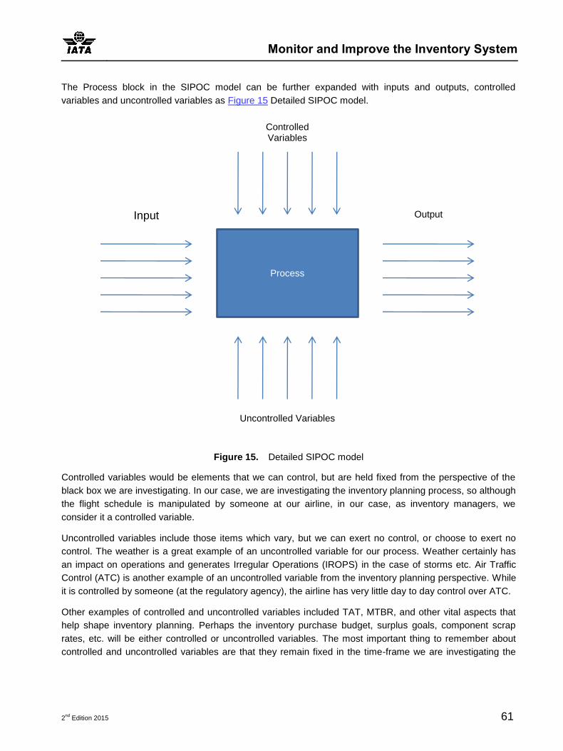
Monitor and Improve the Inventory System
2nd
Edition 2015 61
The Process block in the SIPOC model can be further expanded with inputs and outputs, controlled
variables and uncontrolled variables as Figure 15 Detailed SIPOC model.
Figure 15. Detailed SIPOC model
Controlled variables would be elements that we can control, but are held fixed from the perspective of the
black box we are investigating. In our case, we are investigating the inventory planning process, so although
the flight schedule is manipulated by someone at our airline, in our case, as inventory managers, we
consider it a controlled variable.
Uncontrolled variables include those items which vary, but we can exert no control, or choose to exert no
control. The weather is a great example of an uncontrolled variable for our process. Weather certainly has
an impact on operations and generates Irregular Operations (IROPS) in the case of storms etc. Air Traffic
Control (ATC) is another example of an uncontrolled variable from the inventory planning perspective. While
it is controlled by someone (at the regulatory agency), the airline has very little day to day control over ATC.
Other examples of controlled and uncontrolled variables included TAT, MTBR, and other vital aspects that
help shape inventory planning. Perhaps the inventory purchase budget, surplus goals, component scrap
rates, etc. will be either controlled or uncontrolled variables. The most important thing to remember about
controlled and uncontrolled variables are that they remain fixed in the time-frame we are investigating the
Process
Input Output
Controlled Variables
Uncontrolled Variables

Guidance Material and Best Practices for Inventory Management
62 2nd
Edition 2015
process. Also note that controlled and uncontrolled variables can migrate to the input side of the model if we
choose to vary or change that variable in the time-frame of our continuous improvement investigation.
Since the primary variable we manipulate is whether to stock an item and where, allocation quantities are
great examples of input variables for the planning process. The mix of borrow, pool, lease, exchange and
ownership may also be considered input variables.
Outputs of our inventory management system include DL/CX due to material availability, backorders, service
levels, TDR, etc. The outputs are the first level of measurement we might develop for our metric system
because without it, we would not know how the inventory system we have designed is performing.
Some elements will always be inputs, and some will always be outputs, but some can be open to
interpretation, depending on what element of the process one is currently interrogating. For example, one
may be interested in what impact Rotable service level has on TDR. In this case, Rotable service level might
be considered an input to the TDR output. This example illustrates that there is no hard coded way to design
the system, with a few exceptions (for example, TDR will always be considered an output of the inventory
management system).
Once the system has been modelled as in the discussion above, one is ready to embark on detailed metrics
that can be used to evaluate system performance and begin to improve the output of the planning process.
There are numerous continuous improvement methodologies espoused over recent years. Many have their
roots in manufacturing; however they can be adapted to improving inventory management quite easily. One
example of a methodology is Six Sigma. Consider the following improvement cycle, integral to Six Sigma
improvement:
Figure 16. Typical Six Sigma DMAIC Cycle33
33 For more on Six Sigma, please see (Pande, Neuman and Cavanaugh 2000)
Define
Measure
Analyze
Improve
Control
Monitor and Improve the Inventory System
2nd
Edition 2015 63
This cycle will fit nicely with the 9 step model presented. At the macro level, define maps to understand the
airline’s goals and how the inventory management system fits into the equation. Measure maps to define the
inventory metrics and either measure existing performance, or for a brand new inventory management
system, design a metric system that will allow interrogation of the planning process’ ability to meet the
organization’s needs. Analyse maps to be able to evaluate the performance metrics and whether goals are
being met, and identifying areas for improvement. Improve refers to the process of altering the management
system so that the output of the system as a whole is better. Control refers to being able to hold constant the
variables at the settings we desire so that the outcome of the system is what we expect.
4.1 Inventory Performance Metrics
Inventory Performance Metrics are important because they allow the inventory manager and customer to
gauge performance of the inventory management system. A properly designed set of metrics allow
diagnosis of inventory issues and identification or evaluation of process improvements. Like any system,
inventory management will benefit from a robust process improvement methodology such as Six Sigma, or
similar process improvement methodologies.
Metrics serve to place an objective measurement on the performance of the planning and part delivery
processes. This objectivity is helpful in identifying areas to improve with customers (maintenance and
financial professionals). Metrics are also essential to any planning process.
There are several common metrics that are utilized in evaluation of inventory system performance:
Service Levels
o OOS Events (also referred to as ACOOS Events)
o OOS Elapsed Time (also referred to as ACOOS Elapsed Time)
Fill Rates
Fill Rate = Number of Filled Requests for Parts/Total Parts Requests.
Backorders
o A Backorder is incurred when there is an empty allocation slot in a station.
o Note that healthy material management systems, there will always be backorders as a result of the
removal process at each station. Even with rapid replenishment times (less than 24 hours) from the
main base, a certain number of outstations will always have one too many backorders based on part
usage within the day’s operations.
o In tandem with total number of backorders.
Financial Measurements
Inputs to the Inventory Management System

Guidance Material and Best Practices for Inventory Management
64 2nd
Edition 2015
There are several critical measurements an inventory manager should always track that are inputs into the
system of inventory management. These include the following:
Repair turn time or TAT of each component
o Repair TAT should be monitored for several reasons.
o To ensure it is consistent with planning processes that set WIP levels and station allocations.
Example: Consider a part that is removed 24 times a year (Daily Demand Rate is 0.066). In
Planning a TAT was assumed at 15 days. This resulted in a WIP calculation that required 1 part
for WIP support (for more on calculations, please see Section 6: Understanding Provisioning
Calculations). Now, repair TAT actually has changed to 30 days, resulting in the need for 2 parts
in WIP support. If the airline owned a total of 5 parts, and allocated 4, the second WIP support
spare would come from one of the allocated stations. The practical result is on average, one
station will carry a backorder 365 days a year, and depending on the criticality of the part and
removal patterns, a significant risk to aircraft service level has been created.
o To ensure inconsistent repair times do not invalidate planning assumptions, TAT standard deviation
or at least range should be monitored.
o A large standard deviation in repair times or an Not to Exceed (NTE) can have the same impact as
a shift in average TAT. Similar to the example above, if a TAT of 15 days was assumed in planning
as a NTE TAT, because the arithmetic mean was calculated as 15 days, but the range of actual
repair times is 10 to 30 days, then there will be enough occasions where the actual repair time
exceeds the 15 day assumption and may pose significant ACOOS risk if the part in question is flight
critical. If it is not flight critical, then the absence of the part could still drive up Deferred Maintenance
or MCO balance.
o Many find graphical analysis of component repair TAT’s to be instructive and very useful. Often via
graphical analysis, asymmetric or skewed repair times, large standard deviations, multi-modal
distributions and other phenomena may be quickly observed via use of a histogram.
Scrap Rates of each component
o Scrap rate can fluctuate just as any other quantity used in planning. For example, a unit, due to a
reliability issue, age or another cause, may develop a 25% scrap rate. If this occurs, every fourth
unit that arrives at the shop will require scrap buyback, and in this case, the replenishment lead time
could far exceed the customary repair TAT.
Replenishment Lead Times
o RLT is important when parts must be bought either due to aircraft damage, scrap, demand
increasing due to changes in reliability (decreased MTBF), increased TAT or expanding operations
(increased demand due to opening new stations or expanded service). Many components can be
available immediately on the surplus market. Others may be available in as removed condition, but
serviceable or overhauled may take another 30 to 60 days. Often, new parts from an OEM can have
a short replenishment lead time, but it is not uncommon for major structural components to have
extensive lead times greater than six months.

Monitor and Improve the Inventory System
2nd
Edition 2015 65
No Fault Found Rates
o If a component experiences No Fault Found (NFF), then generally the part is tested, deemed
serviceable and returned to inventory. A high NFF rate will not only tax the logistics system
unnecessarily due to excessive inventory movements, but will also artificially inflate the inventory
balance. NFF is the planning opposite of inflated TAT.
Example: If a repair TAT is assumed to be 15 days, and there are 100 removals annually, then
WIP support would be calculated as 4 units ((100 removal s per year/365 days per year)X15
days). However, if NFF is 75% and the test and return to service is 5 days, then 2 units should
be sufficient for WIP support (( (25 *15)+(75*5))/365)) = 2.05).
Service Levels, Fill Rates and Back orders are interconnected and should be evaluated in conjunction for a
total picture of inventory performance.
Service level is defined as the percentage of time the aircraft are in service due to parts provision, or the
inverse of OOS events. Service level is the inventory related aspect of Technical Dispatch Reliability (TDR).
Interesting Metric Occurrences in inventory management systems:
It is possible to have 100% service level with less than 100% fill rate
o Example: 100 requests for parts in a day’s operations, with 5 no-fills, or a 95% fill rate. However, all
5 no-fills were for parts placed on Deferred Maintenance list or MCO and each aircraft was
dispatched on time.
It is possible to have a large number of backorders however, no impact on aircraft service level:
o Example: 100 part numbers are allocated in a quantity of one each to a station, however, 50 of
those parts are not flight critical (No-Go or Go-If). Any subsequent request can be placed on
Deferred Maintenance list or MCO and filled at a later time, or another location. Note that one of the
luxuries of aircraft inventory management is that both the parts required and the requesting entity
(the aircraft) are mobile. Often this advantage is utilized by moving the aircraft to the part rather than
vice versa, accomplishing the flight schedule in the process.
o Example: 500 part numbers are allocated to a main base, however, only the top 100 part numbers
see more than 2 removals per year. Therefore, the other 500 part numbers can on backorder more
than several months with no impact to service level because there is not another request within the
12 month period.
Example of Rotable inventory performance metrics:
To evaluate the level of service provided in regards to Rotable components there are a couple of things
that need to be decided on prior to starting measurements.
In this example we intend to measure the service level for components that have been defined as No-
Go items and will potentially ground the aircraft.
The service level is measured from the airlines main hub where majority of its maintenance activity
takes place.

Guidance Material and Best Practices for Inventory Management
66 2nd
Edition 2015
The airline owns its Rotable components and has a basic normal set up in regards to purchase, repairs,
exchange and loans or borrow.
It is operating a single fleet type. The airline has assigned 190 components as No-Go items. And a
combined total removals or failures among those 190 is 2689 for 1 year.
Now the next thing is to set the targets. Realistically having all these components in stock all the time and
still run an economical inventory is not possible. So we decide that our service level is to be 90%. So at the
time of our measurements our goal is to have 90% of the 190 components on stock and that the sum of their
1 year removal is 10% or less. Now let’s set this up in a table to review.
No-Go list Jan Feb Mar Apr May
Target number of components nil stock 20 20 20 20 20
Actual number of components nil stock 25 18 30 20 19
Service level 87% 91% 84% 89% 90%
Goal # of removals 269 269 269 269 269
Actual # of removals 290 170 250 270 289
Service level 89% 94% 91% 90% 89%
Table 13. Rotable service level
A few things to point out. First it is possible to meet one objective and not the other as the example clearly
shows. An inventory manager needs to be aware of what that means. For instance a few components with a
high number of removals per year will cause the first objective to be obtained but the second not. An
inventory manager should pay close attention to that as the likelihood of those components failing is higher
due to their high removal rate. The second is that when the first objective is not achieved but the second one
is then the opposite of the first scenario exists. It does not mean that there should be no action as that
scenario is advising the inventory manager that a high number of components are nil stock but their
combined number of removals is within our service level goals.
Both of these indicators should be monitored and addressed accordingly.
Other interesting notes about inventory metrics:
An inventory system with zero or very few backorders is likely over-allocated and carries too heavy
balance for operations. The level of inventory should be investigated for surplus opportunity.
Station by Station comparison can also be used to re-distribute inventory where it will be most utilized.
o Example: If Station A carries very few backorders, has a high service level and a high fill rate, while
Station B carries many backorders, has a lower service level and a lower fill rate than Station A,
inventory re-assignment from Station A to Station B should be investigated. The inventory
Monitor and Improve the Inventory System
2nd
Edition 2015 67
reassignment has the potential to boost the overall performance of the system by increased service
level from Station B while Station A may remain constant.
As already stated, it is possible to have a high aircraft service level with lower than 100% fill rates. High fill
rates generally guarantee high service levels, except in a few special cases that require significant
maintenance time, or special procedures, training, etc. for installation. Examples include: Fuel tank entry,
window replacement (or any other operation required long cure times or long removal and installation steps),
maintenance procedures which require trained personnel only found at certain locations (e.g. flap rigging).
A savvy inventory manager will capitalize on a relationship with maintenance partners, defining maintenance
capabilities as a step in the allocation process. For example, if an engine change is required in a station,
often an engine change crew may route from another location to the station where the aircraft is OOS. In
allocating expensive assets such as engines, the inventory manager can take into account elapsed travel
time plus the removal step to account for when the part to be installed will actually be needed.
4.2 Metrics and their Importance to Operations
In general, it is thought that excessive backorders (BKO) lead to no-fills which will then lead to service
degradation such as high Deferred Maintenance list or MCO count, high MEL count, passenger
inconvenience (example: inoperative lavatory). Impacts can range from special routing of aircraft to address
maintenance issues, restricting aircraft operations, or blocking out seats or zones of seats, restricting
ETOPS operation, delays and cancellation of flights and ultimately extended ACOOS time due to lack of
parts or awaiting parts shipment from another location.
Given the magnitude and breadth of the potential ill-effects of backorders, it is no wonder most inventory
and maintenance managers become concerned when backorders seem to be high. Certainly the
maintenance customer base will react adversely when backorders rise or stay at high levels.
Several metrics can be thought as leading indicators of pending trouble in the inventory management
system. Backorders are obviously one; however the duration of backorders should be taken into
consideration as well. In a large inventory system supporting a large fleet, there will always be a perpetual
minimum number of backorders that may number into the hundreds with no ill effect on system
performance. Of more concern in a large system would be part numbers which spend a large percentage of
the calendar year on backorder. This points to several potential conditions which should be investigated:
The WIP formula should be re-calculated to ensure adequate WIP support spares.
TAT could have increased from the repair source, thus invalidating the previously planned WIP level.
Changes in operations or part reliability could have changed the demand profile, causing annual
removals to spike or permanently change, again invalidating the WIP level.
Conversely, if there is an inventory system where there are zero backorders, expect the Finance
Department to begin questioning allocation and ownership levels. Finance Managers will generally keep an
Guidance Material and Best Practices for Inventory Management
68 2nd
Edition 2015
eye on inventory turns and low turn items, or a low inventory turnover number for the balance as a whole will
invite questions. For this reason, it is recommended the inventory manager track turns and turnover as well.
Traditional Inventory Turnover is calculated as such:
One can imagine that in a Rotable inventory environment there are some issues with this basic formula.
First, the formula was designed to measure inventory that is designed to be sold and leave the firm, which is
the usual manufacturing application. However, for an airline, the basic business model of repair results in
essentially re-manufacturing the same assets over and over again, and the assets remain on the company’s
books in perpetuity. Second, there is no true “Sales” figure expressed in dollars.
At the micro-level, it is valid in a repair process to evaluate how many inventory turnover on a part number
by part number basis. For example:
Example: Assume 25 removals per year and a total spare level of 5 throughout the year
Which is, in reality a very respectable inventory turn number in aviation; further it can be shown that
ownership or full-time leasing of an asset is justifiable if Annual Inventory Turns is greater than 1.0. Consider
that most Finance Managers are educated for manufacturing environments where turnovers are expected to
be much higher, a dim view is taken of aviation inventory turns and other asset utilization metrics such as
Asset Turns.
Practical experience indicates that due to the nature of airline operations, it is not uncommon to have
inventory turnover measured very close to 1.0, sometimes slightly less, sometimes slightly more. The
primary reason is the existence of No-Go inventory which generally must be held in multiple locations in
order to protect operations.
4.3 An Integrated Approach for Metric Monitoring
4.3.1 Frequency
At least monthly: Each inventory manager or supervisor should monitor their respective metrics within
the month as well.
Less frequent than monthly may result in missing important shifts in performance. Remember that the
purpose of measurement is not only to assess system performance, but to correct deviations or system.

Monitor and Improve the Inventory System
2nd
Edition 2015 69
4.3.2 Format
A formal review of metrics on the monthly calendar is prudent, otherwise there may not be adequate
organizational discipline to maintain effective metric review. Often, the managers responsible for the
inventory system will gather and review with one another current and historical performance. It would be
wise as well to include you maintenance suppliers and customers in discussions at least quarterly.
It can be difficult to discern much information from a table of numbers, therefore graphical analysis is
recommended. Graphical analysis may be as simple as plotting histograms and run charts, however it is
recommended that the firm apply Statistical Process Control (SPC)34 or similar methodology such as Six
Sigma to their metric analysis.
When choosing graphical analysis methods, be sure to evaluate whether it is feasible to continually monitor
the metrics put in place. Otherwise, if a metric system is too cumbersome to produce or inaccurate, it will
likely fall into disuse. Additionally, if the metric system is too generic, a manager will not be able to use the
information to diagnose any issues with the inventory system.
At the minimum, a prudent inventory manager would maintain data and metrics so that the following could
be monitored:
Delays and Cancellations attributed to part availability.
ACOOS Event and Duration of each OOS event (or perhaps total ACOOS time).
Fill Rate (the number of filled requests divided by total number of part requests).
Backorders or Rotable Service Level (the inverse of Backorders, defined as total number of assets
currently stocked versus number of allocated assets).
Measuring system metrics is important, as is station level metrics of the same type.
Example: Measure overall system fill rate as well as fill rate on the individual base and station level. If
there is a decline in fill rate, it can be detected if it is a system failure or isolated to certain
locations.
Further, if an issue is suspected at the system or station level, analysis to isolate and diagnose the issue
should be conducted. At this point, the manager may depart into more detailed analysis that is repeated on
the monthly cycle only if a detrimental issue is detected.
Pareto analysis at the station or part number level will graphically isolate the opportunities (stations, part
numbers) for improvement. The first step would be to order data from greatest to least and plot on a Pareto
chart. If stations are being plotted then one might plot no-fills by station, perhaps adjusted for flight activity.
Example: System fill rate has declined and the airline stocks 7 stations. Each station has a varying level of
monthly flight activity so measuring no-fills only could be misleading. Measuring and plotting no-
fills per 100 departures might be a better way to compare station to station.
34 For a treatment of SPC please see (Hines and Montgomery 1990)
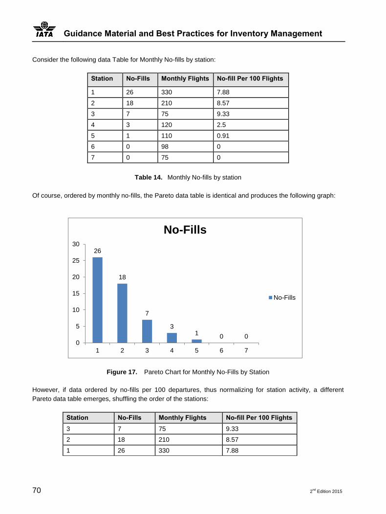
Guidance Material and Best Practices for Inventory Management
70 2nd
Edition 2015
Consider the following data Table for Monthly No-fills by station:
Station No-Fills Monthly Flights No-fill Per 100 Flights
1 26 330 7.88
2 18 210 8.57
3 7 75 9.33
4 3 120 2.5
5 1 110 0.91
6 0 98 0
7 0 75 0
Table 14. Monthly No-fills by station
Of course, ordered by monthly no-fills, the Pareto data table is identical and produces the following graph:
Figure 17. Pareto Chart for Monthly No-Fills by Station
However, if data ordered by no-fills per 100 departures, thus normalizing for station activity, a different
Pareto data table emerges, shuffling the order of the stations:
Station No-Fills Monthly Flights No-fill Per 100 Flights
3 7 75 9.33
2 18 210 8.57
1 26 330 7.88
26
18
7
3 1
0 0 0
5
10
15
20
25
30
1 2 3 4 5 6 7
No-Fills
No-Fills
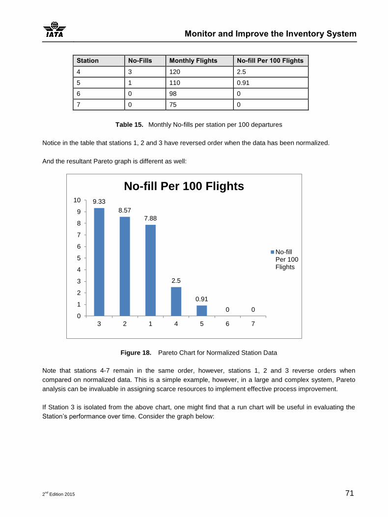
Monitor and Improve the Inventory System
2nd
Edition 2015 71
Station No-Fills Monthly Flights No-fill Per 100 Flights
4 3 120 2.5
5 1 110 0.91
6 0 98 0
7 0 75 0
Table 15. Monthly No-fills per station per 100 departures
Notice in the table that stations 1, 2 and 3 have reversed order when the data has been normalized.
And the resultant Pareto graph is different as well:
Figure 18. Pareto Chart for Normalized Station Data
Note that stations 4-7 remain in the same order, however, stations 1, 2 and 3 reverse orders when
compared on normalized data. This is a simple example, however, in a large and complex system, Pareto
analysis can be invaluable in assigning scarce resources to implement effective process improvement.
If Station 3 is isolated from the above chart, one might find that a run chart will be useful in evaluating the
Station’s performance over time. Consider the graph below:
9.33
8.57
7.88
2.5
0.91
0 0 0
1
2
3
4
5
6
7
8
9
10
3 2 1 4 5 6 7
No-fill Per 100 Flights
No-fillPer 100Flights
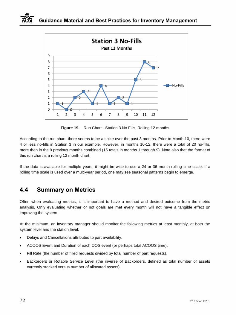
Guidance Material and Best Practices for Inventory Management
72 2nd
Edition 2015
Figure 19. Run Chart - Station 3 No Fills, Rolling 12 months
According to the run chart, there seems to be a spike over the past 3 months. Prior to Month 10, there were
4 or less no-fills in Station 3 in our example. However, in months 10-12, there were a total of 20 no-fills,
more than in the 9 previous months combined (15 totals in months 1 through 9). Note also that the format of
this run chart is a rolling 12 month chart.
If the data is available for multiple years, it might be wise to use a 24 or 36 month rolling time-scale. If a
rolling time scale is used over a multi-year period, one may see seasonal patterns begin to emerge.
4.4 Summary on Metrics
Often when evaluating metrics, it is important to have a method and desired outcome from the metric
analysis. Only evaluating whether or not goals are met every month will not have a tangible effect on
improving the system.
At the minimum, an inventory manager should monitor the following metrics at least monthly, at both the
system level and the station level:
Delays and Cancellations attributed to part availability.
ACOOS Event and Duration of each OOS event (or perhaps total ACOOS time).
Fill Rate (the number of filled requests divided by total number of part requests).
Backorders or Rotable Service Level (the inverse of Backorders, defined as total number of assets
currently stocked versus number of allocated assets).
1
0
2
3
1
4
1
2
1
5
8
7
0
1
2
3
4
5
6
7
8
9
1 2 3 4 5 6 7 8 9 10 11 12
Station 3 No-Fills Past 12 Months
No-Fills

2nd
Edition 2015 73
Section 5—Understanding Provisioning Calculations
This section is intended to give a deeper understanding of the inner workings of airline provisioning theory
and calculations. While dealing heavily in statistical concepts, this section is not intended as a mathematical
proof, but rather a presentation of a widely accepted and proven method of airline inventory provisioning.
5.1 Assumption of a Poisson Process
Fundamental to airline provisioning calculations is the assumption that failures of the components of the
aircraft follow a Poisson Process. A Poisson process is one of the most important counting processes. We
use it to estimate removal volume and inter-arrival times of removals. A Poisson Process has some
important characteristics:
Each event is Independently, Identically Distributed (IID).
o We shall discuss Identically Distributed first. In practical terms, each unique MPN on the aircraft has
its own operational characteristics, including an inherent failure rate. The Poisson Process does not
delve into complex multiple regression models or infinite computer simulation to develop a model
and estimate for removals. Instead, we use the simple assumption that any pump or generator or
APU or engine or actuator will behave like any part with the same MPN.
o Independently Distributed is a very important characteristic for us. In practical terms, independently
distributed components are removed according to a common rate (identically distributed) but do not
depend on when the last removal occurred, either on the aircraft or within the same MPN family. For
example, failure of a center wing fuel pump may be considered to occur with a MTBR of 10,000
hours. Each identical fuel pump in the fleet will behave according to this MTBR. However, the failure
of pump serial number 1 does not have any impact on when serial number 2 fails.
The expected number of removals can be estimated by the following equation:
o [ ( )]
o The above equation is the foundation for estimating future removals based on flight hours and
MTBR.
The Poisson process has what is known as a “memory-less” property. This comes about because of the
Independently Distributed events that make up the process. As described in 1b above, the failure of
serialized parts are independent of one another, linked only by their shared failure distribution.
While this guide is not intended to be a statistical treatise, some readers may find additional reading
desirable. If so, there are many texts regarding Poisson processes, some of which are detailed in the
bibliography of this guide.

Guidance Material and Best Practices for Inventory Management
74 2nd
Edition 2015
For the airline inventory manager who can either bring to bear a background in probability and statistics, or
take the calculations presented herein on faith, this guide should provide enough substance to allow for
trouble free application of the provisioning calculations.
5.2 Notes on Essential Data and Sparing Calculations
The essential data elements for sparing calculations:
Number of aircraft
o The total number of aircraft to be supported by fleet.
Aircraft Utilization (usually expressed in hours per day)
o For some parts, such as wheels/brakes, or landing gear, utilization should be expressed as cycles
per day. However, note that if the hours-to-cycle ratio is always constant, flight hours can be
substituted for cycles.
QPERAC
o Refers to the quantity of a specific part number installed on each aircraft. For example, the same
hydraulic pump may be installed on 4 separate positions per aircraft, 2 active and 2 standbys. Note
that positions are often identified by an Aircraft Location Number (ALN).
MTBR
o Refers to Mean Time Between Removal, usually expressed in hours. Note that MTBR can be
calculated using total hours flown and total removals.
Example: If Total Annual Removals were 5 for a certain part, and fleet hours totalled 100,000
hours for the year MTBR would be calculated as follows:
o For some parts, such as wheels/brakes, or landing gear, if utilization is expressed in cycles, then be
sure to calculate MTBR in cycles.
o MTBR is specific to each part number.
o In some cases manufacturers will express MTBR as total removals per 1000 hours.
o Further, for instances where we use for calculations on individual parts,

Understanding Provisioning Calculations
2nd
Edition 2015 75
To calculate Annual Demand (D),
The output of the calculation will be removals per year, by part number. This number is essential in
calculating spares needed to cover the repair process time (Turn Around Time or TAT) that is experienced
on each part. Annual Demand (D) corresponds to the annual removal rate.
To calculate daily demand (dd), simply eliminate the 365
Or alternatively, if Annual Demand (D) is already calculated, then
Calculating Annual Demand (D) is fundamental to understanding spares and spares allocation for WIP and
for station support. Some general rules to consider:
For Annual Demand less than one per year (D<1), consider alternatives to ownership or full-time leasing
such as pooling, borrow strategies, or exchanges, based on criticality of the part(s) in question:
o For No-Go parts (CAT 1), consider pooling partnerships, or locate an airline partner willing to loan
parts to your airline in the event of an unscheduled removal.
o For Go-If parts (CAT 2) again consider pooling partnerships and borrow partners. The primary
difference between pooling and borrow arrangement is payment. Pooling is usually accompanied by
an access or membership fee per aircraft or station and is paid regardless of usage, often through a
clearinghouse. Borrowing can be considered a spot market, paid at the time of use and based on
the duration of use. Note that neither pooling nor borrowing necessarily implies a service level or fill
rate guarantee on the part of the provider.
o For all other parts (CAT 3) that can be logged as Deferred Maintenance or MCO, consider
exchange programs or perhaps stocking a limited number of parts at a main base only. Because
aircraft can be dispatched with CAT 3 parts inoperative, it is reasonable to forego allocation to any
station except the main base.
For Annual Demand much less than one per year (D<<1), consider taking calculated risks that might
include borrow, pool or exchange strategies discussed elsewhere in this guide.
5.3 MTTR or TAT
Often an inventory manager is faced with the question of whether to use a statistically derived MTTR or a
more subjective TAT.

Guidance Material and Best Practices for Inventory Management
76 2nd
Edition 2015
When considering the following equation,
TAT is preferred to MTTR because MTTR can mislead one regarding the expected repair time on a
population of parts. MTTR should be evaluated either graphically using histograms or numerically using
statistical calculations. Comparisons of the mean to the median to the mode can also highlight issues that
may need to be addressed by graphical analysis. Finally, the standard deviation of repair times should be
investigated since highly variable repair times can cause issues if a static TAT is assumed. A manager can
investigate many part numbers by using a spreadsheet format, highlighting only those part numbers that
show problematic behaviour.
TAT is a target set not necessarily with arithmetic or statistical methods. TAT is often treated as an NTE
goal, and many contracts with suppliers refer to TAT.
Utilizing an average TAT measurement (or MTTR for that measure) can lead to disastrous planning
implications since the average is, by definition, only “Right” 50% of the time.
5.3.1 Using MTTR in Lieu of TAT
MTTR can be used with a right skewed repair distribution. A quick check is Mode<median<mean.
Remember that Mode is the most frequently occurring number in a data set. The median is the point at
which 50% of the data lies above and 50% lies below, and the mean is the arithmetic average.
Since the average can be arithmetically inflated by a long “tail” to a distribution, using average MTTR can
sometimes work well with a right skewed TAT. However, when using a right skewed TAT be aware that
inventory balances will be inflated due to an overestimate of the TAT via the mean.
Figure 20. Right Skewed Distribution

Understanding Provisioning Calculations
2nd
Edition 2015 77
The greater the separation between median and mean, the more comfortable one can be using a right-
skewed MTTR. Another way to deal with a right skewed MTTR histogram would be to throw out the value(s)
that make up the long tail, assuming there is justification to discount these repair times. For example, if a
typical repair time is 27 days, ± 7 days, but there are several 200+ day repair times known, if those 200 day
repair times were invalid as uncharacteristic for some reason (perhaps accomplishment one time of an
Engineering Order (EO) for example), then the 200+ day TATs could be cut from the data set used to
calculate average TAT.
Average TAT is not recommended for use for symmetrical distributions, nor for left skewed distributions. Left
skewed distributions are frequently subject to the exact opposite convention regarding the tail as right
skewed TATs. With left skewed TATs, the majority of the repair times are long, and when plotted on a
histogram with a tail stretching back to zero for a few infrequent quick turn repairs or tests. This tail
stretching back to zero has the effect of artificially deflating the MTTR. Thus, if one uses average MTTR in
provisioning calculation, a detrimental portion of data will be excluded from the NTE TAT, resulting in stock-
outs and service interruptions.
Figure 21. Left Skewed Distribution
From the NIST,
A symmetric distribution is one in which the 2 "halves" of the histogram appear as mirror-images of one
another. A skewed (non-symmetric) distribution is a distribution in which there is no such mirror-imaging.
For skewed distributions, it is quite common to have one tail of the distribution considerably longer or drawn
out relative to the other tail. A "skewed right" distribution is one in which the tail is on the right side. A
"skewed left" distribution is one in which the tail is on the left side. The above histogram is for a distribution
that is skewed right.35
35 (“HISTOGRAM INTERPRETATION: SKEWED (NON-NORMAL) RIGHT”, NIST/SEMATECH E-HANDBOOK OF STATISTICAL
METHODS, http://www.itl.nist.gov/div898/handbook/eda/section3/histogr6.htm, October 23, 2008)
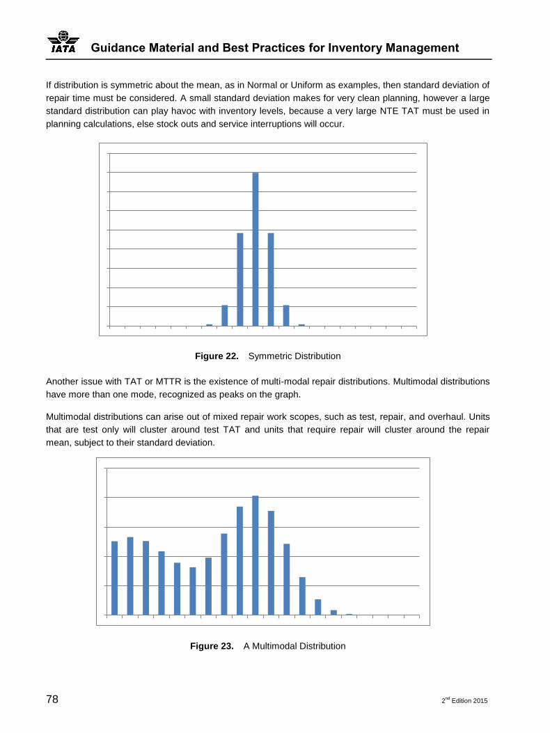
Guidance Material and Best Practices for Inventory Management
78 2nd
Edition 2015
If distribution is symmetric about the mean, as in Normal or Uniform as examples, then standard deviation of
repair time must be considered. A small standard deviation makes for very clean planning, however a large
standard distribution can play havoc with inventory levels, because a very large NTE TAT must be used in
planning calculations, else stock outs and service interruptions will occur.
Figure 22. Symmetric Distribution
Another issue with TAT or MTTR is the existence of multi-modal repair distributions. Multimodal distributions
have more than one mode, recognized as peaks on the graph.
Multimodal distributions can arise out of mixed repair work scopes, such as test, repair, and overhaul. Units
that are test only will cluster around test TAT and units that require repair will cluster around the repair
mean, subject to their standard deviation.
Figure 23. A Multimodal Distribution

Understanding Provisioning Calculations
2nd
Edition 2015 79
5.3.2 Summary of MTTR Versus TAT
When establishing TAT to be used in the WIP calculation, take care to analyse averages before they are
used in the calculation. It is important to understand the characteristics of the underlying repair distribution,
including the shape, standard deviation, and existence of multiple modes. Graphical analysis using
histograms will highlight any potentials issues, and usage of control charts or at least a run chart should be
employed to ensure that the repair time is performing the same over time.

Guidance Material and Best Practices for Inventory Management
80 2nd
Edition 2015
Section 6—Forecasting, Practical Application and Impact on Sparing Strategy
Regardless of whether one uses very rigorous quantitative methods to derive a removal forecast, or perhaps
less scientific but still effective qualitative methods, there will always be a human element in the
determination of spares levels.
Truly there are some very useful probabilistic methods to determine unscheduled removal volume driven by
the various failure modes of the various components. However, extensive mathematical modelling of failure
modes and the inherent variation can result in a model which performs well historically, but can be of
misleading value in forecasting future removals.
In the practical application, often the best forecasting approach is accurately model the macro situation with
a human adjustment if necessary. This statement may make forecasting purists cringe, however it is borne
out by experience. Often forecasts can be created with various methods which predict annual volumes with
acceptable error, however, these same forecasts can break down miserably when annual volumes are
divided into monthly or weekly requirements.
Only the most stable performing components lend themselves well to a forecast that can be safely
depended upon for monthly or weekly spare requirements. Often aircraft components behave in very
irregular patterns, are sometimes subject to seasonality, and there can be tremendous variation in monthly
requirements, playing havoc with the supporting spares pool.
In essence, sparing for airline operations is like buying insurance. The level of insurance taken is related to
the desired risk level borne. In this case, each spare purchased or accessed via leasing or other methods is
an insurance policy against an AOG for that part. The risk incurred is the out of service time awaiting a part.
The risk can be small if the part is stocked in each operational station, but this can carry a heavy financial
premium. The risk can be larger if a removed part must be shipped from another location, or even must be
procured first (via purchase, lease, borrow, exchange), and then shipped into the required location.
Some carriers are extremely conservative in their operational strategy, abhorring any delay related to spare
assets, and consequently carry very large inventory balances. Other carriers take a very conservative
financial approach, treating inventory investment as an absolute minimum, and thus incur what might be
undue risk in operations, offsetting the savings in inventory with operational cost.
It is recommended to take a balanced approach, crafting a strategy that takes acceptable risk at low cost to
the airline, and mitigates higher levels of risk with a spare procurement strategy blending multiple
provisioning methods (ownership, lease, borrow, exchange). In this way, an airline can expect satisfactory
operational performance at the lowest total cost.

Forecasting, Practical Application and Impact on Sparing Strategy
2nd
Edition 2015 81
6.1 Day to Day Operational Considerations
The inventory manager in charge of planning and procuring assets should think of the airline’s AOG Desk as
a customer. If a thorough job of planning is done prior to the handoff to Logistics, filling daily requirements
should be smooth and efficient. Examples include:
Having pooling relationships established and communicated with the AOG Desk.
Having all borrow contracts and credit checks completed ahead of time so the AOG Desk only has to
source the part from a pre-established borrow partner.
Providing the AOG desk with options or a play book, including which airlines or providers have inventory
stocked in locations the airline will serve.
If key parts are expected to be procured via pool, borrow or exchange, highlight these for the AOG
Desk.
Communication with the AOG Desk, as with Maintenance partners will be critical in achieving the goals set-
out for the inventory system. The AOG desk is often the inventory manager’s greatest ally and a good AOG
desk that has been included in the planning process and armed with information can make the inventory
manager’s system design look brilliant, even in times when that design might be a little short.
6.2 Surplus
Surplus aircraft parts can be readily available on the market since most airframes have a long service life of
perhaps two decades or more. Surplus can be used to an airline’s advantage, both by reducing procurement
cost versus purchasing new parts, as well as allowing the airline to divest itself of excess assets.
6.2.1 Surplus of Excess Assets
In the course of operations excess inventory can become available in response to decreases in demand.
The sources of decreased demand can vary from completion of aircraft modification, fleet retirement or
reduction in fleet numbers, improved component reliability (changes in MTBR), reduction in scrap rates,
reduction in fleet utilization, or other reasons. If the change in demand is deemed permanent, then the
inventory manager is faced with inventory on the balance sheet that is suddenly excess to the operation.
In this situation, a well-established surplus operation can be a great asset to the inventory manager. The
surplus operation can be internal to the airline, or provided by a vendor or partner.
Within the airline, a few personnel dedicated and knowledgeable of the surplus market can return many
times their cost in revenue that might otherwise be missed. In addition, a healthy surplus operation can help
reduce the inventory balance, keeping it right-sized for the airline operations, and generate savings in taxes
and insurance costs that are tied to the value of the inventory balance.

Guidance Material and Best Practices for Inventory Management
82 2nd
Edition 2015
Depending on the fleets and fleet plans at the airline, the revenue from a healthy surplus operation can
offset new inventory purchase by as much as 100% or even double or triple the annual purchase plan,
resulting in an overall balance reduction while keeping service levels high.
There are several options for surplus that may be right for the airline’s operations:
A full-time internal department which handles surplus activity on a continual basis. If the airline’s surplus
activity is heavy enough, this can be a viable and lucrative option.
Occasional auctions of surplus material can be scheduled if surplus activity is not as regular and may be
event driven (i.e. fleet retirement, occasional aircraft modification, reduction in utilization, etc.) Some
airlines choose this option and the auction is often coordinated internally by the inventory management
department. This option can be successful if there is infrequent (perhaps quarterly) need to divest the
airline of excess assets.
Partnership with a broker or other firm specializing in surplus assets. This option can take the form of a
full-time relationship, or in lot sales, auctions, or consignment sales by the partner. The inventory
department’s planners must still designate inventory as excess, and perform surplus transactions,
however the partner activity may range from full-service to merely a marketing arrangement that entails
calling the airline when one of the partner’s customers is looking for a specific part on surplus. Often this
option can be a hybrid solution that can be catered to fit the airline’s needs for surplus activity.
Many airlines acquire spare engines when they purchase aircraft. Often, a portion of these engines will be
idle for a large percentage of the calendar year. Leasing of idle engines should present a revenue
opportunity that can exceed $1M revenue per engine per year. To illustrate the revenue possible, consider a
CFM56-7B engine being made available for lease.
Key Assumptions:
Each month an engine is rented, either whole or partial, the following fees apply.
Monthly Lease Rates
Monthly Low Estimate
Monthly High Estimate
Monthly Average Rate
$ 83,000 $ 105,000 $ 94,000
Table 16. Lease Rates
For the purpose of the calculations we will use the $94,000 Monthly Average.
Also, to accrue a maintenance reserve against the usage of the engine, additional charges for hours and
cycles are as such:
Monthly Lease Rates
Monthly Estimate Low Monthly Estimate High Monthly Average Rate
$ 83,000 $ 105,000 $ 94,000

Forecasting, Practical Application and Impact on Sparing Strategy
2nd
Edition 2015 83
Hour/Cycle Charges
Hour Charge Cycle Charge
$ 126 $ 83
Daily Fees
Hours (6) Cycles (4) Total
$ 756 $ 332 $ 1088
A/C Utilization
Hour Assumption Cycles
6 4
Table 17. Charges
So for each day that the engine is used by a leasing customer, $1,088 in fees will be accrued, assuming the
6:4 hour to cycle ratio.
If we then calculate that the engine will be leased to a customer between 3 and 9 months per year, (3
months - 25%, 6 months - 50%, 9 months – 75%), we can produce the following:
Table 18. Revenues
The annual revenue estimates are based on the engine assets only being leased 25% to 75% of the year,
which is a very conservative approach. Often an engine can be leased to a single customer for an entire
year. If however, the engine asset is leased to multiple customers, the 50%-75% revenue assumptions are
feasible, even with return and re-marketing of the engine during the year.
6.2.2 Purchase of Assets on the Surplus Market
Since there can be significant surplus assets available for multiple fleet types at any given time, it would be
wise to have a robust surplus purchasing option available when the need to buy inventory arises.
There can be some disadvantages to surplus inventory, but a properly designed surplus purchasing
program can prevent these issues. Issues may include concerns about quality or safety of surplus units. To
combat safety or quality issues, many airlines compile an Approved Surplus Supplier list to enter into
Lease Fee Model
Engine Number of Engines Leased
Monthly Rental Average
Daily Hour and Cycle Charges
Percent of Year Leased
Expected Reserve Hour and Cycle Charges
Total Annual Revenue Estimates
CFM56-7B 1 $94,000 $1,088 25% $381,494 $99,494 $ 480,988
CFM56-7B 1 $94,000 $1,088 50% $762,987 $198,987 $ 961,974
CFM56-7B 1 $94,000 $1,088 75% $1,144,481 $298,481 $ 1,442,962

Guidance Material and Best Practices for Inventory Management
84 2nd
Edition 2015
partnership with one or many providers of surplus parts. Another option to insure that the airline is
purchasing a valid part is to get a copy of the certificate and the traceability papers.
The advantages of utilizing surplus parts are two-fold. The first advantage is obviously cost savings. Every
year, OEM catalogues customarily revise CLP for the parts they manufacture. Often these revisions are
based on the CPI and can increase 3% or more year over year.
An inventory manager may find a need for a particular MPN that can be bought both from the OEM as well
as from the surplus market. While it is true that an airline may have preferred pricing in place with the OEM,
the surplus market may have the same part available in serviceable condition for as little as 20% or 30% of
CLP. Overhauled parts will bring more of a premium, but they will still likely be cheaper than CLP. Certain
fleets, due to recent teardowns of aircraft or announced fleet retirements may have a flood of inexpensive
parts on the market. Other fleets due to their popularity or relative youth may demand a price much closer to
CLP, but still a 10% to 20% savings can be had. Also, the inventory manager should keep in mind that there
are cross-effective parts between fleets, and the price may be less on surplus due to activity on one or more
of several fleets, even if the manager is buying for a newer model.
The second advantage is in immediate availability. Often OEM parts go directly to aircraft being built, or
there may be significant lead time from an OEM to purchase a new part. If an airline has an AOG situation,
or other immediate need, a 45-day lead time from the manufacturer will not help. Often the same part can be
found for immediate availability with a broker or surplus partner in serviceable or overhauled condition.
Having surplus purchase as an option can offset potentially long lead times that may adversely affect
operational metrics.
If an active surplus-buying mechanism does not currently exist at the inventory manager’s airline, it is
recommended to partner with the Quality, Maintenance, Finance, and Supply Chain/Purchasing
Departments to investigate the savings that surplus material can offer an airline.
6.3 Airline-MRO Relationships
Recent trends show that many airlines are adopting a partnership with an MRO provider. These
relationships may extend into how inventory is treated between the partners.
The most common inventory partnership between and airline and an MRO affects WIP inventory. Because
often the MRO has complete responsibility for TAT on component repair, it is natural to enter into some sort
of WIP inventory arrangement with an MRO.
Consider that since WIP = Demand X TAT is a direct relationship between TAT and WIP, that any increase
or decrease in TAT will affect WIP significantly. If TAT increases by 50%, say from 30 to 45 days, then the
inventory manager should expect that the WIP requirement will also increase 50%. If this increase is a result
of awarding business to an MRO, or perhaps pre-existing business and changes in TAT, it is reasonable to
approach the MRO about some type of WIP support partnership. Conversely, if the airline can negotiate a
reduction in TAT, the same reduction in WIP support can be expected.
Forecasting, Practical Application and Impact on Sparing Strategy
2nd
Edition 2015 85
Most common with MRO providers is a guaranteed TAT with some sort of provision to pay for borrow activity
incurred by the airline if TAT is missed and an AOG situation arises while the part in question is late out of
repair. These agreements can be on a part by part basis, but may be more commonly expressed as a
certain percentage of parts will be returned within the NTE TAT by the vendor. For example, a vendor may
commit to 95% of all repairs completed within 30 days TAT.
An inventory manager should be aware of the contractual obligations of the vendor, and should calculate
risks associated with vendor non-performance. For example, with the aforementioned 95% NTE TAT goal
mentioned above, if the volume is 100 parts per month, the vendor can be late with 5 parts with no penalty.
This would mean that the inventory system would not only potentially have some AOG situations to for
which to provide parts, but that contractually the costs are fully borne by the airline. Further the inventory
manager should consider focusing on getting the service level applicable only or mainly on those parts
which are considered No-Go. For example an airline does a component service agreement for 200 MPN
with a 95% service level. The normal situation would be where the complete list is dealt with on the 95%
service level. For an operator to get better service it would be good to consider breaking the part number list
up based on how critical the parts are to the operation. Parts that would fall into No-Go and Mel A category
should get a higher service level and on the other spectrum parts that are less critical could get lower
service level. This way the operator gets the highest level of service for the most critical parts. The value of
this needs to be determined on each case as the higher service level requested the higher the cost. An
inventory manager can use a number of tools to assess the situations, such as probability and the
calculation outlined in this guide to estimate the risk associated with vendor contracts.
Of course it is possible that an MRO may completely provide the physical assets for airline operation. An
MRO may agree to provide either via exchange or pooling for the WIP required to support the sparing
process, however the station inventory is still owned by the airline.
Going one step further, a MRO or partner may provide fully the station support inventory (allocated
inventory) as well as WIP inventory driven by the repair process and TAT.
Complete provision of inventory assets is most often the case through an inventory pooling solution offered
by an MRO or other partner. A common pooling arrangement creates a mechanism where the MRO or
inventory partner agrees to provide a part to the operator at one or many locations within a certain period of
time. Often AOG events are given very strict time lines whereas non-AOG may have several days or more
to provide the airline with a requested part. Conversely, the airline must agree to provide the unserviceable
removed part back to the pool provider so the repair pipeline is primed and the replenishment/repair process
can proceed in a timely fashion. If this type of arrangement exists, all calculations in this guide are still valid,
the only difference being who is providing the inventory as the owner of record. Logistics time should also be
accounted and planned for in this type of model.
One can imagine how pooling is an excellent concept to explore since there are so many parts that can
negatively impact operations if they are not available, but are only required very infrequently on an annual
basis. Consider an international station such as JFK in New York, LHR in London, or CDG in Paris; each of
these stations has numerous operators operating daily flights. Every one of these operators desires to have
a high service level into these stations, which will drive everyone to provision some of the same inventory at
levels they have calculated. However, what to do when a $200,000 part shows one usage a year in the

Guidance Material and Best Practices for Inventory Management
86 2nd
Edition 2015
station? The most obvious answer would be to combine or aggregate demand with the expensive part so
that rather than for example four operators each allocating one $200,000 part to JFK, the four operators can
cooperate and share in one or two parts, reducing the value of the inventory on the field by up to a factor of
four, or at worst, halving the total investment on field to $400,000 (2 units at $200,000 each).
There are disadvantages to pooling also:
Seasonality for the parts in question should be investigated. For example, if hydraulic part numbers are
pooled, then winter MTBR should be used to ensure adequate assets for all sharing partners.
Over-conservative airlines tend to worry that when they desire a part, then it is not available due to a
very aggressive airline or airlines abusing the pool. This concern can be addressed by monitoring NFF
and limiting pool usage to failure only. Airlines can be forbidden from drawing on pool inventory for
scheduled or time control removals, and tracking NFF will highlight whether an airline may be
troubleshooting with parts simply because they are available in the pool.
Some other considerations for airline-MRO relationships:
The inventory manager should track TAT whether the repair is internal or external. The WIP calculations
are sensitive to changes in TAT, and if a major shift occurs, a drastic increase in station backorders can
occur.
MTBR should be monitored as well for changes in reliability, either increased or decreased. Increases in
MTBT could highlight surplus opportunity while decreases in reliability will result in increased demand
and could require increases in both station and WIP inventory if erosion of part reliability is left
unchecked.
If an inventory manager is used to the flexibility and convenience of internal shops, be mindful that the
contractual terms will likely be filled. For example, if prior TAT experience with an internal shop was 15
days NTE for planning usage, and an Outside Repair (OSR) contract is signed with a 30 day NTE TAT
guarantee, expect to plan at the new TAT.
MRO relationships can be as beneficial to the airline and the inventory management system as internal
relationships. Inventory managers are encouraged to cultivate the same communication level with external
providers as with internal maintenance.
6.4 Inventory Sale-Leasebacks
Inventory sale-leasebacks occurs when an airline decides to sell its inventory to a vendor who will keep all
or a portion of it available to the airline, usually via a lease fee. Airlines may decide to reduce the inventory
balance for a number of reasons:
Generate cash from the sale of inventory.
Fleet retirement in the industry will result in loss of inventory value for the airline.
The aircraft parent asset is leased for a fixed period of time.
The airline’s fleet plans have a definite horizon that makes leasing attractive.

Forecasting, Practical Application and Impact on Sparing Strategy
2nd
Edition 2015 87
New arrangements in repair reduce TAT so that a portion of WIP can be reduced.
Contraction or consolidation in the airline network reduces the number of allocated stations.
Often inventory sales are consummated for the simple reason to generate cash flow. If there are no other
driving forces, such as a change in demand, the airline will require the inventory footprint currently held to
remain in place. If the inventory is required for any reason of the sale, then a leaseback is put in place.
Usually, the transaction is financial only, with the title passing from the airline to the new lessor, and the
inventory physically never changes hands at the lease inception.
In cases where the fleet plan of the airline is on a fixed horizon, or industry fleet retirements are announced,
or any other internal or external fleet change occurs, the assets the airline owns will deflate in value.
Depending on the age of the fleet, the airline’s inventory acquisition value, and the depreciation schedule, a
market-driven change in salvage/surplus value of the firm’s assets may cause the inventory balance to
decrease to the point where it is at or below the airline’s book value of the inventory. If the inventory is sold
below book value, a loss will be incurred. It is wise in these situations to pursue a sale-leaseback in order to
capitalize on the value of the inventory ahead of any events that will deflate the inventory value.
In cases where a change in maintenance affords a TAT reduction or changes in the network decrease the
need for the current level of station allocation, a sale of surplus assets can be entertained. If the change in
demand may not be permanent, a sale-leaseback allows the airline to enjoy the cash infusion of the sale,
but maintain the flexibility and access with a lease. Often, reduction in TAT or changes in network can
generate a partial sale of inventory, however many vendors or leasing partners will find the surplus inventory
tantalizing and the idea of a lease for the balance of the needed inventory will be very palatable to a number
of potential business partners.
6.4.1 Some Specifics Regarding Sale-Leasebacks
The inventory manager and other airline personnel may question how a sale-leaseback could be profitable
for a partner unless that partner has some nefarious designs on the inventory as a whole. The answer to the
question lies in the cost of capital. Most airlines have a relatively high carry cost, approaching or even
exceeding twenty percent. Much of this carry cost consists of the airline’s cost of capital. Due to the state of
airlines in the economy today and the perception of risk by the financial community, airlines will typically pay
a high rate of interest on any use of capital. Aviation is very capital intensive, whether for new aircraft
acquisition, upgrades to existing fleets or facilities, or purchase of inventory to support a new fleet. An airline
will almost always have numerous capital projects which must be funded.
Conversely, there are private and public equity firms, and companies whose business entails brokering
aircraft parts that have a lower cost of capital than the airlines. Even though both the airline and the partner
may pay the same amount in taxes and insurance as well as the other costs that make up carry cost, the
difference in cost of capital is often significant and will make the sale and purchase a good decision by the
airline and its chosen partner.

Guidance Material and Best Practices for Inventory Management
88 2nd
Edition 2015
Inventory sale-leasebacks can take the form of a 100% sale and leaseback, or a 100% sale and partial
leaseback. The full leaseback scenario will occur when an airline requires the entire inventory sold to the
partner for operations. There may be a definite term on the lease, coupled with fleet retirement or other
known events which reduce the demand for the parts over time. For example, a firm may operate 20 aircraft
that will be phased out of the fleet on a 5 year schedule. Inventory to support the fleet will be required until
the last aircraft ceases operations. If the airline held the inventory in ownership until the retirement, the value
on the market would depress for the airline and the salvage value may even fall into single digit
percentages. By partnering with a fully-informed vendor, the airline can negotiate a sale price and
subsequent lease which can capture more of the current market value of the parts. The airline and vendor
may also design a contractual arrangement that allows for additional surplus parts to be removed from the
lease arrangement over time, freeing the parts for immediate disposition on the market by the vendor.
A full-sale and partial leaseback will generally occur when a portion of the vendor’s inventory is deemed to
be immediately surplus to operational needs; however the remainder will be necessary to sustain
operations. As demonstrated in the section regarding Purchase versus Lease, long term leases can be more
competitive with purchase than common sense might dictate. An similar NPV analysis on sale-leaseback
versus maintain ownership can be conducted that shows a long-term lease is competitive versus maintain
the inventory until it is 100% obsolete to the airline’s needs. These types of leases are attractive to vendors
since they will realize not only a continuing lease payment from the airline, but also have inventory they can
immediately broker. Like the 100% sale-leaseback, the airline and vendor may also design a contractual
arrangement that allows for additional surplus parts to be removed from the lease arrangement over time,
freeing the parts for immediate disposition on the market by the vendor.
When negotiating a sale-leaseback, keep in mind that the two critical elements are the sale price/acquisition
value, and the lease rate. If the airline demands current market price for all inventory in negotiation, the
lease rate will also be based on the partner’s market value acquisition from the airline. If a lower acquisition
is negotiated, the long-term lease payments will be lower as well. The entire transaction can be endangered
if the airline is insistent on market value sale, then shocked at the price of the annual lease. Rather than
abandon the idea, the airline should realistically investigate what surplus value will be when the airline holds
the inventory to the very last. Sensitivity analysis coupled with NPV analysis can help the airline decide
where the walk-away point should be in the negotiation. Be careful to assume realistic surplus value-airlines
typically do not receive good value for their parts once the market is aware of a demand change. A
recommended approach would be to negotiate a sale price and lease rate that is palatable to both firms,
with the recognition that negotiation failure will result ultimately in a de-value of the airline inventory in the
future.
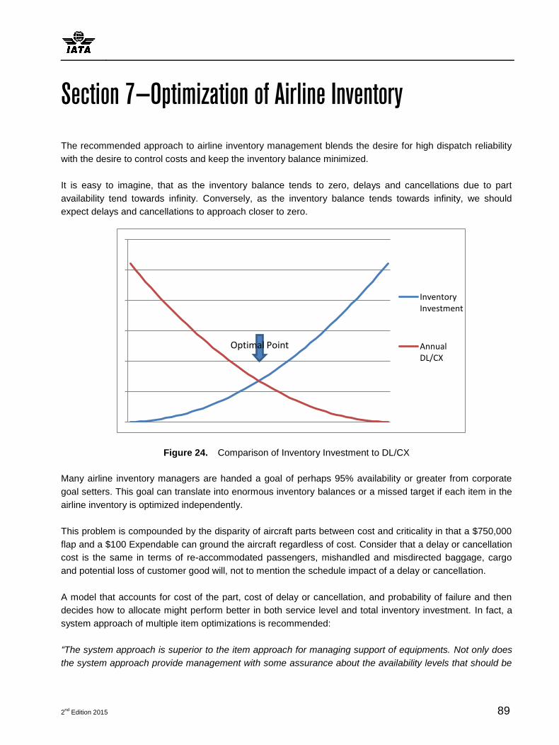
2nd
Edition 2015 89
Section 7—Optimization of Airline Inventory
The recommended approach to airline inventory management blends the desire for high dispatch reliability
with the desire to control costs and keep the inventory balance minimized.
It is easy to imagine, that as the inventory balance tends to zero, delays and cancellations due to part
availability tend towards infinity. Conversely, as the inventory balance tends towards infinity, we should
expect delays and cancellations to approach closer to zero.
Figure 24. Comparison of Inventory Investment to DL/CX
Many airline inventory managers are handed a goal of perhaps 95% availability or greater from corporate
goal setters. This goal can translate into enormous inventory balances or a missed target if each item in the
airline inventory is optimized independently.
This problem is compounded by the disparity of aircraft parts between cost and criticality in that a $750,000
flap and a $100 Expendable can ground the aircraft regardless of cost. Consider that a delay or cancellation
cost is the same in terms of re-accommodated passengers, mishandled and misdirected baggage, cargo
and potential loss of customer good will, not to mention the schedule impact of a delay or cancellation.
A model that accounts for cost of the part, cost of delay or cancellation, and probability of failure and then
decides how to allocate might perform better in both service level and total inventory investment. In fact, a
system approach of multiple item optimizations is recommended:
“The system approach is superior to the item approach for managing support of equipments. Not only does
the system approach provide management with some assurance about the availability levels that should be
InventoryInvestment
AnnualDL/CX
Optimal Point

Guidance Material and Best Practices for Inventory Management
90 2nd
Edition 2015
attained, but any specified availability is achieved at dramatically lower investment. This has been
demonstrated repeatedly both in computer simulations and actual field tests over a period of 25 years.”36
The problem as a Linear Program37 could be stated as such:
∑
And some the constraints might be:
Where SL is system service level, Y is the service level goal, B is inventory balance, and X is the balance
goal or limit given by Finance. Equations would have to be developed by the manager that would define the
interrelationships and flesh out the model.
This type of model would work well for a start-up operation, however if an airline already has existing
inventory, it may give either a mathematically infeasible result or tell the inventory manager that the airline
has all the wrong parts in all the wrong places.
Models that account for a starting point in inventory are necessary when an airline already owns inventory.
While the results from an optimization model can be used to validate (or invalidate) the items that are
stocked, often an optimization model does not account for the disparity between sale of surplus inventory
and the purchase price of items needed.
A solution for the custom developed model could be worked on a small scale by a solver in commercially
available spreadsheet programs. Commercially available mathematical software can handle larger
problems. Finally, there is commercially available software that addresses specific solution for industries
such as airlines, shipping, railroad, etc.
The manager should keep in mind that any optimization model is only as good as its inputs, so clean and
accurate data are essential to producing reliable results. Further, the system must be maintained and will
require management at each schedule change.
Finally, at best, the model results should be cross-checked with human intelligence to ensure that
operations will be covered. The manager should be able to explain model results and decisions taken from
the output.
36 P.17 (Sherbrooke 1992)
37 For more on Linear and Mathematical Programming, please see (Winston 1991)
Optimization of Airline Inventory
2nd
Edition 2015 91
Linear programs are not the only models that will provide the manager with some intelligence about the
inventory management system. Simulation can be a powerful tool in evaluating decisions, particularly
wholesale changes to inventory systems.
If the manager is faced with choosing between two or more disparate inventory strategies, a simulation can
help choose the relative goodness between each of the options under consideration. Like Linear Programs,
or any other model, care should be taken in literally applying results of simulation to real-world expectations.
Since the simulation is a model that depends on its representation of reality as well the data inputs, directly
applying simulation results to real-world goals or commitments should be avoided.
For example, if a simulation model is created to determine whether a better service level is achieved by
dispersing or consolidating inventory, and respectively generate a 91% and a 98% service level, the
manager would choose the 98% service level option, but committing to the airline that a 98% service level
would be achieved might be overestimation, unless the simulation completely and accurately modelled
every aspect of real operations.
Nonetheless, simulation can be a very powerful tool when applied properly, and unless the manager is
versed in simulation techniques, consulting with simulation professionals is recommended.
7.1 Goals Revisited with Optimization
There are generally two opposing schools of thought in airline spares management which give rise to a third,
blended approach. The first goal that surfaces is maximizing dispatch reliability, and usually leads to very
large inventories to support the goal. The second goal is minimizing investment in airline inventory and
usually is at odds with the first goal since maximizing dispatch reliability leads to inflated inventory balances.
The third goal emerges out of the relationship of the first two and results in the optimization of operational
parameters. This optimization is a blended approach, taking into account the factors or dispatch reliability
and financial investment.
The goal of airline inventory management is very simply stated as maximizing part availability at the lowest
total cost. While simple in concept, the execution can become quite complex. Consider that most aircraft
consist of tens of thousands of parts an inventory manager is faced with making the correct decisions on
stocking for Expendables and Rotable/Repairable parts.
With both Expendables and Rotables/Repairables, the first decision a manager must make is whether to
own a part or not. This is often referred to as designating a part as a Stock Item or NASI. Many stock items
are clear decisions as to ownership, as factors such as removal or failure rate and criticality of the part (No-
Go, Go-If, Go). It is almost a given that if a manager expects several removals a year on a No-Go part that it
will be designated a stock item.
After deciding whether an item is a Stock Item or NASI, then a manager must begin a more complex
process which involves the flight schedule, number of maintenance bases, number of main bases (or
stations) and the criticality and failure rates of the parts of interest. This quickly can become a complex
calculation that can be sub-optimized if what is known as Single Item Optimization is used. Single Item

Guidance Material and Best Practices for Inventory Management
92 2nd
Edition 2015
Optimization is exactly what it implies-each item is evaluated separate from all other parts on a set of criteria
that results in a decision for that specific part. A manager would then proceed step-wise through the desired
parts list until all parts have been evaluated.
Single Item Optimization is not a recommended approach simply because it often results in inflated
inventory balances. Several factors combine to make Single Item Optimization sub-optimal. First, a manager
is generally given a goal of “system” part availability. If for example a goal of 95% part availability is given, it
is generally understood as 95/100 requests for a part are successful.
The next logical thought would be multiple item optimizations, which would account for the fact that a
manager can achieve an overall 95% fill rate by compromising on some parts and overstocking on others.
However, once again multiple item optimizations may result in inflated inventory balances. For example, a fill
rate of 85/100 on one part could be offset by a fill rate of 97/100 on 5 other part numbers. The overall fill rate
would be 570 of 600 requests, or 95%.
Expendables stocking is usually a fairly straightforward matter relative to the stocking of Rotable and
Repairable parts, even in only a single location or station base. Expendables are usually treated with the
well-known and generally accepted EOQ.
For parts which have a repair process, the pipeline inventory (parts in the repair process), as well as station
allocations (parts held at forward stocking locations to facilitate availability) becomes more complex as one
has to account for the repair process.
Every item or part, whether Expendable (Consumable) or Repairable (Rotable/Repairable) contributes to the
overall success of creating an acceptable part availability and also contributes to the sum of financial assets
committed to inventory. As such, it is recommended that some approach be taken that incorporates a
system view of inventory.
In acquiring a system view, the articulation of goals becomes paramount. For example, is a 95% availability
rate applicable to the whole system in aggregate, or is the 95% availability rate required at each station?
Usually a station specific allocation and stocking program will result in more inventory than a system which
provides for a 95% aggregate fill rate. It is possible to have the same number of fills, say 950 of 1000
requests, and at a single 25 of 25 requests result in no fill, therefore at the station level, the 95% availability
rate would be a failure.
7.1.1 Organizational Structures
When designing the organizational structures for inventory management, there are some questions the
inventory manager should consider. In recent years, regulatory action such as Sarbanes-Oxley has brought
approval processes to the forefront. An organization can be in compliance with regulations as long as a
clearly defined way of doing business is documented and followed. The process should include and adhere
to approval limits and processes. For example, the following approval processes may be required:

Optimization of Airline Inventory
2nd
Edition 2015 93
Buyer Authorized to Purchase up to: (in USD)
Approval required Next Level Approval
Inventory Planner $25,000 Manager Signature above $25,000
Manager
Inventory Manager $100,000 Director, Finance and Director, Inventory Signatures Above $100,000
Director, Inventory
Director- Inventory $500,000 Controller, and VP-Maintenance signatures required above $500,000
Vice President-Maintenance
Vice President-Maintenance
$1,000,000 Chief Operations Officer & Controller signatures above $1,000,000 and less than $2,500,000
Executive Committee for any purchase exceeding $2,500,000
Table 19. Example Approval Levels for Inventory Purchase
These limits are usually per purchase. For example, during the day a planner may buy 4 components (each
a different MPN) for scrap replacement at $20,000 each, totalling $80,000 but a manager’s signature will not
be required. However, if the inventory manager has procured a lease of $250,000 operating expense per
year to lease parts required to cover new service, it is recommended to aggregate the expense and seek the
Director level approval required.
The impact of recent regulation has been that the buyer cannot also be the approver of the same purchase.
So even if the inventory planner is purchasing a component that is $10,000, well under the planner’s
spending limit, another party usually must authorize the Purchase Order (PO) before it can be sent to a
vendor.
As a result, many airlines have an organizational structure similar to one of the following models:
Inventory Analysts are buyers and planners, and have full purchase capability including sourcing and
negotiation with vendors
o Purchase Orders will be approved by Finance or Supply Chain, but the inventory planner and
manager provide all data-the approval is merely for oversight.
Inventory Analysts are planners only, providing part numbers and quantities to another element of the
organization to purchase
o The buying activity, including sourcing and negotiating with vendors, will take place in Finance,
Supply Chain or Purchasing.
Beyond the purchasing function, there are a number of ways that the organization can be structured. Often
airlines will delineate responsibility by ATA chapter, by inventory type (Rotable or Expendable), by
application (airframe inventory versus engine inventory), or by customer base (planners for line
maintenance, base maintenance, and repair support).
Guidance Material and Best Practices for Inventory Management
94 2nd
Edition 2015
While each method of organization has its own distinct advantages and disadvantages, some guidelines for
structure can help the inventory manager decide how to design the organization to best deliver great
service:
The expected workload should be balanced among the available inventory planners.
o Most airlines publish multiple schedules per year. These may include significant changes in
utilization, equipment and destinations from schedule to schedule. Evaluating parts for allocation is
just as time consuming for high volume parts as low volume.
o Scrap activity should be taken into account as well, since high usage parts with a scrap percentage
will generate constant buyback activity.
o Airlines with multiple fleets may delineate analysts by fleet, however be careful that the workload is
balanced for the analysts.
If a logical balance by fleet cannot be attained, perhaps an ATA structure can be easier managed
o Metrics for the individual analysts should follow their organizational structure
For example, if fleet metrics are used, but inventory planners are organized by ATA chapter,
then the fleet metrics should be sub-grouped into ATA chapter as well so the metric analysis
and system performance can be meaningful at the planner level.
Planners (and managers) should be encouraged to partner with their maintenance customers and
providers. For example, if a planner has responsibility for wheels and brakes for all fleets, then building
a relationship with the wheel and brake shop as well as with line maintenance personnel may yield
planning dividends. Throughout this guide there are situations highlighted where cooperation with
maintenance personnel would be a good practice. If line maintenance understands the allocation
rationale, and the repair shops are brought into the decision process, the synergy can be powerful. For
example, if a planner has responsibility for wheels and brakes for all fleets, then building a relationship
with the wheel and brake shop as well as with line maintenance personnel may yield planning dividends.
An increase in demand may not only result in inventory purchase, but perhaps there is a shop
improvement project that is almost complete that will reduce TAT, obviating the need for increased WIP
inventory.
Things to avoid:
o In general, there should be a one-to-one relationship between planners and part numbers. It is
generally unwise to break up part number responsibility between multiple planners.
o Unbalanced workload should be avoided as well. As in all endeavors, a manager should be able to
assess that each planner has a roughly equivalent workload. This becomes especially important
during each schedule change.
o Planning in isolation-maintenance providers and maintenance customers will have a wealth of
information, technical knowledge and improvement ideas that can positively impact the planning
process and the output of the inventory management system as a whole.

Optimization of Airline Inventory
2nd
Edition 2015 95
7.2 Interactions an Inventory Manager Should Expect
In the course of day-to-day operational concerns, monthly or quarterly planning and allocations, or for
annual budget process, the inventory manager should expect interactions with people within and outside the
organization. Interfacing successfully with each constituent is as much the key to success in inventory
management as it is with any organization. Often the inventory manager deals with very definitive
mathematical equations, but at the end of the day, the people both within and outside the organization are
the most important elements to achieving the goals desired.
Figure 25. Internal Interactions
7.2.1 Internal Interactions
Internal interactions will be daily to weekly frequency. An inventory manager should expect the following
situations and interactions with internal parties:
AOG Desk
o Conversion of customer borrows to exchange or purchase: the AOG desk will usually be the
customer-facing element of loan/borrow transactions and if a customer requests a loan be
Spares Planning
AOG Desk
Logistics / Stores
Quality & Receiving Inspection
Maintenance Planning
Loans & Borrows
Finance Supply Chain Management
Engineering
Maintenance
Maintenance Control Center
Surplus Sales
Guidance Material and Best Practices for Inventory Management
96 2nd
Edition 2015
converted to an exchange or outright purchase, the spares manager should be consulted for
approval of the transaction.
o Stock-outs or increases in use: the AOG desk is the front-line representative of the entire inventory
management system, dealing with maintenance every minute of the day. There will be times when
they notice emerging trends and can alert the inventory manager to changes in spares demand.
o At schedule change, when the airline alters flight patterns, hours and even fleets in a region, the
AOG desk should be advised of upcoming material movements. The AOG desk should also be
given the opportunity to comment on the upcoming changes and provide advice based on their
experience. Often the inventory manager and AOG desk can collectively discover solutions and
breakthroughs by drawing on one another’s experience and expertise.
o The inventory manager should cultivate a good relationship with the AOG desk personnel. The AOG
desk makes the inventory system work by making decisions to tactically move spares from their
stocking location to the place where maintenance will install the part. In this way, the AOG desk
enhances the designed performance of the inventory system. By partnering with the AOG desk and
including them in the process of planning and evaluation of the inventory system, the inventory
manager can expect better results.
Logistics/Stores
o The logistics and stores arm execute the plan, in conjunction with the AOG desk.
o While the logistics and stores personnel are executing every day of operations, the main interaction
with planning occurs at flight schedule change. Logistics personnel and management should be
advised by the planning department as to the magnitude of the inventory movements required to
accommodate the new schedule. In addition, stores personnel will use the schedule change
information to evaluate the warehousing capacity in each station and make changes as necessary.
Quality and Receiving Inspection
o Interactions with the quality department and receiving inspection arise generally associated with
asset acquisition. Assets can be acquired via purchase, lease, borrow or exchange, and there can
be times where an incoming part will be stopped at receiving inspection and the buyer will become
involved to clear receiving. Many airlines operate with approved parts providers to minimize issues
at receiving inspection.
Maintenance Planning
o Maintenance Planning and Spares Planning often work in conjunction with one another.
Maintenance Planning departments are usually charged with oversight of timing and work package
coordination for required checks for the fleet of aircraft. Maintenance planning will set up a schedule
for the accomplishment of time-controlled removals and EO modifications to the aircraft. Since many
of these campaigns require spares to accomplish, close coordination between Maintenance
Planning and Spares Planning is essential to accomplish all work on time with lowest total cost.
o It is recommended that the Spares Planning manager cultivate a good relationship with the
Maintenance Planning personnel. Frequent interactions will assist both parties to achieve their
goals.

Optimization of Airline Inventory
2nd
Edition 2015 97
Loans and Borrows
o Often the spares planning group will have responsibility for loans and borrows as well. Loan volume
(uses by other airlines) should be taken into account for spares planning. In addition, borrow activity
(quantity of parts provided by other airlines) should be monitored to ensure that the costs of borrow
are in line with usage and do not warrant the purchase of another spare.
o If the loans and borrows are administered by a group outside planning, then frequent
communication and data monitoring of loan and borrow activity are necessary.
o Loan and borrow tactical activity and operations will include the AOG desk and logistics/stores
personnel.
Finance
o Finance interactions should permeate every aspect of spares planning since the relationship
between asset investment, service levels, and budgetary constraints is paramount in inventory
management. Close relations with the Finance department can foster a spirit of cooperation and can
result in better overall performance of the inventory system, in both service level and financial
measures.
Supply Chain Management
o Spares planning will often interact with Supply Chain Management (SCM) since purchasing material
is often a daily activity for the planning department. In some organization, the supply chain
management personnel or purchasing personnel are charged with oversight of the planning
purchases to ensure integrity of the process. In addition, there may be PO approval levels that
require release from SCM. Often, if very large purchases are made, SCM personnel may coordinate
the vendor relationships and selection processes.
Engineering
o Spares Planning and Engineering will be involved with quality and reliability investigations. For
example, if MTBR for a certain part is degrading, spares planning should notify the engineering
section for an investigation and corrective action. It can also be that the reliability section of the
engineering departments notices a change in MTBR and notifies spares planning. Also, engineering
and spares planning will often coordinate with maintenance personnel to assign the cause of an
aircraft delay or cancellation charged to the maintenance division. In addition, Engineering will
initiate actions such as modifications that will result in spares requirements and will thus require
spares planning involvement.
Maintenance
o Maintenance interaction will be almost daily as line or hangar maintenance personnel are truly the
customers of spares planning services. It is important to maintain a good working relationship with
maintenance in order to understand fully their requirements and needs and also to share information
regarding spares planning. Maintenance events such as station openings and closings have
profound effects upon inventory levels. Maintenance personnel should also be consulted during
planning processes as elements such as mechanic qualification, maintenance elapsed times and
other factors can influence how material is allocated to support maintenance activity.

Guidance Material and Best Practices for Inventory Management
98 2nd
Edition 2015
Maintenance Control Center
o The airline’s MCC is a tactical entity involved with the day to day operations of the aircraft. Usually
the AOG Desk will take care of all the interactions with the MCC, however there may be times
where meeting with maintenance personnel in the MCC is wise. An Example would be coordination
between spares planning, maintenance planning and the MCC on a campaign to remove and install
a fleet-wide modification.
Surplus Sales
o In the course of spares planning, surplus assets will be identified. Many airlines operate a surplus
sales group in order to dispose of the surplus assets and capitalize on the value of the parts.
Whether the surplus item sales are on an individual basis, or selling of an entire fleet of inventory,
coordination with surplus sales will be necessary. Spares planning analysts will often discuss and
facilitate paperwork issues with surplus sales personnel, and should also advise the surplus
personnel in advance of quantities and part numbers of assets to be sent to the surplus warehouse
so the receiving and quality inspection processes can go smoothly.
7.2.2 External Interactions
External interactions can be numerous and frequent or might be encountered only sparingly. It is not
uncommon for spares managers to interact with one another from across the aviation spectrum. Attending
meetings such as IATP Pooling conferences, or other formal gatherings give spares managers the chance
to interact and discuss vital aspects of inventory provisioning. Borrow and pooling strategies employed as
parts of the overall inventory provisioning solution will provide many opportunities with peers from other
airlines.
Spares managers are often included in sourcing investigations and decisions and will be able to interact with
MROs, IT vendors and leasing companies. In the course of loan and borrow administration, loan customers
and borrow providers from other airlines are frequently encountered.
OEM interactions may occur when new fleets are being added to the airline, as well as during upgrade and
modification of components flown on the existing fleet. In the case of quality or reliability degradation, the
spares manager will encounter OEM interaction in conjunction with the airline’s engineering section.

Optimization of Airline Inventory
2nd
Edition 2015 99
Figure 26. External Interactions
7.3 Expendable Planning
7.3.1 Introduction
Expendable planning can be thought of as perhaps simpler than Rotable planning since Expendables have
some key characteristics that are different than Rotables:
Expendables exit the inventory planning system at consumption
o Since Expendables have an assumed 100% scrap rate, and are consumed at the time of use, an
inventory manager does not have to plan for the repair cycle.
o However, in the repair cycle discussion of WIP and DD and TAT, the same formulas may be used,
as we shall see, by replacing TAT with RLT.
Individual Expendables are generally low cost items in comparison with Rotables. Average Price of
Rotables may range in the $20,000-$40,000 USD with perhaps a max of $300,000-$750,000 (avionics
computers and flaps, for example). Expendables on the other hand may very typically be only a few
dollars each, or even cents (Example: fasteners, gaskets, seals etc.); however, there are Expendables
that may range up into the $5,000 USD range (sensors or certain filters).
Spares Planning
Other Air Lines
IATP
MROs
IT Vendors
Leasing Companies
Loan Customers
Borrow Providers
OEM
Third Party Logistics

Guidance Material and Best Practices for Inventory Management
100 2nd
Edition 2015
Generally, Expendables are one-time use items, with no repair capability. In some events, a repair can
be made available for an Expendable; for example a test and return to serviceability of sensors; certain
filters may be cleaned and returned to service.
Expendables are generally expensed at the time of issue from the warehouse or depot to a station or
location such as a bay. As such, Expendables are not as rigorously tracked after issuance as a Rotable.
In some cases, consumption is assumed and is never tracked after the point of issue from the
warehouse. This is fairly common in airline operations, however, in MRO and repair scenarios,
Expendables may be tracked both financially and operationally down to installation in an Next Higher
Assembly (NHA).
Expendable balances can be burnt down if quantities are too high. As such, “guessing wrong” on
quantities can be mitigated by modifying future orders. Care must still be taken to order the correct part
numbers, however, slight overages in quantities of an Expendable in demand can be offset by careful
management.
Even though Expendable planning is conceptually simpler than Rotable planning and management, it is
equally important since a revenue flight can be just as easily delayed for lack of a low-cost item as it can be
for a $300,000 computer.
7.3.2 Expendable Planning Strategies
There are several ways to consider planning Expendables. Since Expendables are often less-scrutinized by
the internal finance community than Rotables, the methods and strategies for Expendable planning and
management are usually left entirely up to the inventory manager, and can thus be tailored to the needs of
the operation.
With wide-open options for planning and management of Expendables, a manager can select from the
following methods in general, ordered from least to most complex, at the station level:
Method Description Advantages Disadvantages Comments
Single, Identical Complement of Expendables at every station.
Use one set allocation for every station, regardless of station size, fleet, or location.
Ease of planning
Minimal time investment at flight schedule change
Deployment of new stations will not require complex analysis
Known, fixed cost of allocation (one-time expense)
Minimal re-allocation of Expendables from
Not responsive to variation in flight schedule, equipment / fleet, or maintenance capabilities / requirements
May result in under or over allocation if there is significant variation in the
flight schedule
Over allocation will result in slow moving inventory
Can be ideal for single gauge equipment operators (i.e. one fleet) with one to several maintenance stations, all with the same flight frequency and maintenance profile.

Optimization of Airline Inventory
2nd
Edition 2015 101
Method Description Advantages Disadvantages Comments
station to station at schedule change.
and unneeded funds tied up in Expendable inventory balances at stations.
Under allocation can cause delay or cancellation due to inventory availability.
Customized Complement of Expendables.
Similar to 1. Above however, individual stations created and planned accordingly.
Station specific allocations minimize over or under allocations.
Planning time investment increases directly with the number of stations planned
Planning is done as schedule data is known and may be done in a compressed time environment due to the dynamics of schedule change
Deployment of new stations requires understanding the flight schedule and maintenance requirements at a station level.
May be typically used by a single fleet or small multi-fleet operator, with a few maintenance stations and limited station-to-station schedule, fleet and maintenance variations. Practicality lessens when there are frequent schedule changes that significantly modify station requirements.
Tiered Complement of Expendables by station type or station maintenance classification.
A range of station specific Expendable allocations are created for the anticipated flight frequencies, fleets and maintenance requirements.
Pre-planning for Expendable allocation can be accomplished any time and then adapted for schedule change (note schedule change planning is generally time-sensitive)
Can be practical for either large or small carriers with significant station to station flight frequency, fleet or maintenance variability.
Stations must be “bucketed” into the existing tiers or a new tier created, perhaps losing some flexibility.
Some very large airlines have been known to use this method extensively prior to adopting an MRP or Optimization approach. Requires close coordination with maintenance in terms of maintenance capability and intentions at the station level.

Guidance Material and Best Practices for Inventory Management
102 2nd
Edition 2015
Method Description Advantages Disadvantages Comments
MRP MRP-“Material Requirements Planning” is a term borrowed from manufacturing. All Expendables would be considered based on station needs and a recommendation for allocation is generated by the computer system.
Increased cohesiveness with actual flight schedule, fleet and maintenance requirements result in a more optimal allocation of Expendables than prior methods.
Requires an operating system to accomplish the analysis, where all previous examples could be feasibly done in a spreadsheet environment, even for large airlines.
Significant effort is required to model the “real-world” adequately to gain the optimal result from MRP.
Practical only for large airlines in most applications as the cost of software may be prohibitive for smaller airlines, unless software providers change their licensing and pricing models.
Optimization This is a broad category for computer based management of Expendable allocation. Arguably MRP, which typically required computational resources to accomplish, also falls into this category. Optimization essentially means balancing the cost of delays or cancellations with the cost of ownership.
Expendables and Rotables can be allocated together as one financial pool, minimized the total cost of ownership
A good data and model design will approximate airline operations fairly well and result in good operational decisions.
Can be complex and time-consuming to set-up and maintain.
Optimization models are only as good as the data and approach used to approximate the real world.
Multiple software providers claim to offer an optimized solution for Expendables and Rotables.
Table 20. Expendable Planning Methods
Management and allocation of Expendables at the depot or warehouse level is treated slightly differently.
Consider the following model, with 1 warehouse and one up to many stations:

Optimization of Airline Inventory
2nd
Edition 2015 103
Figure 27. Demand from outstations required from Warehouse
The warehouse is aggregating demand from 1 to many stations (3 are shown, however there may be
typically between 5 and 30+ at most airlines).
Each station has been allocated a complement of inventory. We will assume that this inventory is expensed
at the time of use, and that a re-order point has been established and that the re-order process is either
managed manually (i.e. via cycle counting, min bin or Kanban system or similar), or electronically (via an
MRP “Material Requirements Planning” or ERP-“Enterprise Resource Planning”-software.
In the case of the warehouse, one can assume there will be periodic replenishments to each station to cover
usage.
Warehouse inventory may be larger in size, both quantities and financially, than any individual station, but in
a well-managed warehouse, the inventory will move through the warehouse at a faster rate than it will in
stations, generally. This inventory movement is measured in inventory turns, defined as follows:
∑
All Issues will be the financial sum (in USD or local currency), over a period of time (usually one year), for
the entire inventory that was issued from a location. Average Inventory Value will be in the same currency
as issues, and should be the average of values over the same time frame as the issues. Note that inventory
turns will be a unit less number.
Examples:
A Warehouse has an average of almost $50 Million USD in inventory for the entire year of 2014. Calculated
from the following month-end inventory values:
Station 1
Station 2
Station n
Warehouse
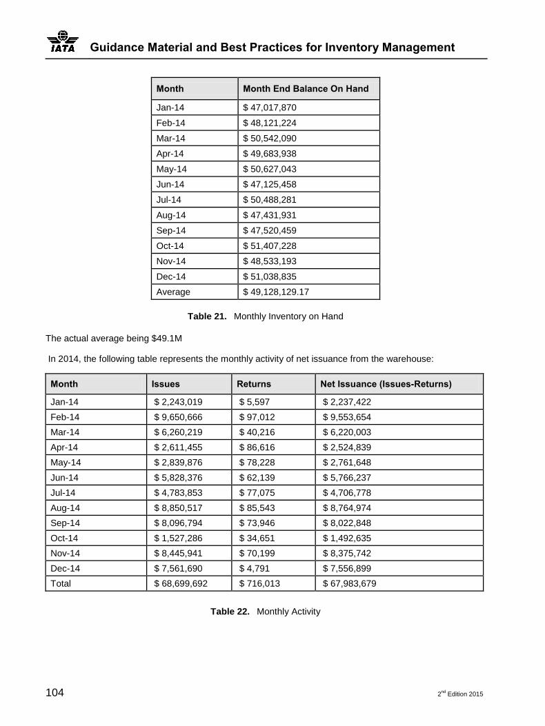
Guidance Material and Best Practices for Inventory Management
104 2nd
Edition 2015
Month Month End Balance On Hand
Jan-14 $ 47,017,870
Feb-14 $ 48,121,224
Mar-14 $ 50,542,090
Apr-14 $ 49,683,938
May-14 $ 50,627,043
Jun-14 $ 47,125,458
Jul-14 $ 50,488,281
Aug-14 $ 47,431,931
Sep-14 $ 47,520,459
Oct-14 $ 51,407,228
Nov-14 $ 48,533,193
Dec-14 $ 51,038,835
Average $ 49,128,129.17
Table 21. Monthly Inventory on Hand
The actual average being $49.1M
In 2014, the following table represents the monthly activity of net issuance from the warehouse:
Month Issues Returns Net Issuance (Issues-Returns)
Jan-14 $ 2,243,019 $ 5,597 $ 2,237,422
Feb-14 $ 9,650,666 $ 97,012 $ 9,553,654
Mar-14 $ 6,260,219 $ 40,216 $ 6,220,003
Apr-14 $ 2,611,455 $ 86,616 $ 2,524,839
May-14 $ 2,839,876 $ 78,228 $ 2,761,648
Jun-14 $ 5,828,376 $ 62,139 $ 5,766,237
Jul-14 $ 4,783,853 $ 77,075 $ 4,706,778
Aug-14 $ 8,850,517 $ 85,543 $ 8,764,974
Sep-14 $ 8,096,794 $ 73,946 $ 8,022,848
Oct-14 $ 1,527,286 $ 34,651 $ 1,492,635
Nov-14 $ 8,445,941 $ 70,199 $ 8,375,742
Dec-14 $ 7,561,690 $ 4,791 $ 7,556,899
Total $ 68,699,692 $ 716,013 $ 67,983,679
Table 22. Monthly Activity

Optimization of Airline Inventory
2nd
Edition 2015 105
To calculate turns we would apply the equation above, and use the example Average inventory as the
denominator, and the sum of the annual issuance as the numerator as follows:
In general, an aviation warehouse turning >1.0 per year is performing fairly well. Persons familiar with
inventory turns from other industries such as manufacturing and retail might be accustomed to much higher
inventory turn ratios. Due to the intermittent demand, turns much greater than 2 are rare and show a well-
managed warehouse assuming that delays and cancellations metrics exceed operational goals.
7.3.3 Planning the Expendables Warehouse
Planning for the warehouse will seem like a large job, but in actuality, it can be quite easy to accomplish.
Consider the following:
The warehouse aggregates demand at one location for all usage in the system. In other words, all
station inventory flows through the warehouse.
Expendables enter the warehouse system at receipt and leave at issuance and usually do not return.
Return of Expendables38, while rare, are usually the result of changes in station allocation driven by
equipment changes.
o For example, a station formerly servicing an all-Boeing fleet that will service only Airbus in the next
schedule might return a significant complement of inventory to be re-deployed elsewhere (assuming
the carrier will still operate Boeing aircraft).
o In another example, a station that formerly serviced all narrow body aircraft, that will as a result of
growth and a schedule change service all wide body aircraft, may require Expendables to be re-
allocated and re-distributed throughout the system.
An inventory manager has the choice to “burn down” Expendable allocations where they may be too
high for local use by carefully metering the re-ordering process. This provides an alternative to returning
inventory to be re-stocked in the warehouse.
o For example, consider that a change in flight frequency results in a reduction in Service Checks and
this Expendable use for service checks at a station. Assume a certain filter is stocked in quantity of
4 at the station due to prior service check intervals. Other assumptions include:
Reorder point was set at 2 units.
Re-order quantity is 3.
RLT is 1 day from the warehouse.
Former filter usage was from 1-3 per week.
New schedule indicates that filter usage will be 3 per month.
38 For Expandable to be returned and accepted back to inventory each operator must make sure it is done in accordance with the rules
and regulation in regards to traceability, quality etc.

Guidance Material and Best Practices for Inventory Management
106 2nd
Edition 2015
The inventory manager may recall some of the 6 filters to re-deploy at another station, or may
choose to allow the 6 filters to remain in place as a 2 month supply, and in this case maintain
the re-order point of 2 filters. Once 2 month’s usage passes, the re-order point will kick-in,
ordering the re-order quantity of 3. From the 2nd
month forward, the maximum number of filters
at the station will be 5 or less.
Alternatively, the inventory manager may decide to adjust both the re-order point and the re-order
quantity. Since RLT is short (1 day from the warehouse), the station may carry a smaller complement of
filters. Note that the warehouse stocks for any long lead time items. Re-order point could be adjusted to
1 or zero units (zero unit re-order point would require a certainty that there will be a max of 1 demand
per overnight service check and that the RLT is truly 1 day or less from the warehouse). Furthermore,
the re-order quantity could also be adjusted downwards to 2 or even 1 per order.
For a planning regimen, the inventory manager can certainly follow the approach laid out of Rotables in
section 4.3 of this document. The nine step model will work fine, provided all the data is available for the
calculations. In addition, the inventory manager should replace Rotable TAT with the Expendable RLT.
Recall that Rotables are subject to a repair cycle governed by TAT, and WIP inventory is calculated to cover
the repair cycle with serviceable units. In the case of Expendables, A comparison of TAT to RLT can be
seen below:
TAT and RLT in Planning
TAT "Turn Around Time"
Warehouse RLT "Warehouse Replenishment Lead Time"
Station RLT "Station Replenishment Lead Time"
Used to cover the repair cycle of Rotables from removal at station to processing at warehouse, the repair itself to make the unit serviceable, and then return the serviceable unit to the warehouse.
Used to represent the time needed to order and receive an Expendable from a manufacturer or distributor.
Used to represent the shorter lead time between station re-order to the warehouse and the logistics time to move the part from the warehouse to the station.
It represents any repair time needed plus logistics time to move the part.
Since an Expendable is not repaired but rather ordered an OEM or distributor, this time represents the ordering, wait time if any for the manufacturer to make or distributor to procure, plus any logistics time.
Stations will typically re-order from the warehouse, assuming the warehouse stocks the item. Since a station is ordering smaller quantities of Expendables, and aircraft Expendable weight and dimensions are typically conducive to air shipment, a carrier will usually ship its own Expendables for replenishment in its own aircraft. For this reason, Station RLTs are typically short.
A typical TAT might be 28-45 days.
A typical Expendable RLT to the OEM or distributor might be 30-120 days.
A typical station RLT is 1 day, depending on flight frequencies.
Table 23. Comparison of TAT of RLT

Optimization of Airline Inventory
2nd
Edition 2015 107
While an inventory manager can certainly follow the nine-step model, a more abbreviated and appropriate
approach for Expendables can be followed. For a station, the process is outlined below:
Figure 28. Expendable Planning Simplified
7.3.4 Planning Station Expendables
In the following discussion we will assume the warehouse has already been set-up. In fact, it’s not really
important whether the warehouse is set-up first or the stations are set-up first. The most important first step
is to determine the stock items.
Figure 29. Setting up Stations or Warehouse First?
We allocate the warehouse based on aggregate annual demand because we are interested in minimizing
the total cost of ownership. See the EOQ in Warehouse Management section for this discussion.
Determine Stock Items
Determine RLT
Set Allocation Quantity
Set Safety Stock or
Min
Determine Reorder
Point and Reorder Quantity
Physically Allocate Inventory
Monitor Inventory Quantity
& Replenish
As Needed
Setting Up Warehouse First
• Determine Stock Items
• Allocate the Warehouse based on aggregate annual demand
• Allocate each station based in station usage
Setting Up Stations First
• Determine Stock Items
• Allocate each station based on station usage
• Allocate Warehouse based on aggregate annual demand

Guidance Material and Best Practices for Inventory Management
108 2nd
Edition 2015
Note that the operations of the airline change significantly at schedule change (either fleet, frequencies, or
maintenance requirements) the station usage should be for the period of the schedule change. See chart
below for guidance.
Schedule Change Provisioning Period Demand
Annually 12 Months Annual usage is used
Bi-Annual 6 months ½ Annual usage, accounting for seasonality39
Quarterly 3 months Use appropriate 3 months usage40
Monthly 1 month Use either a 3 month smoothed average, prior year month usage, or another forecasting method that gives adequate accuracy41
Table 24. Guidance for Schedule Change Demand
7.3.4.1 Data Needed
To plan a station, the inventory manager will need to have the following data on hand:
Part number
RLT – Replenishment Lead Time in Days
Safety Stock –Can be calculated-please see section below on Calculating Safety Stock
Desired In-Stock Percentage
Daily Demand
7.3.4.2 Calculating Safety Stock
Safety stock describes the level of extra Expendables that is maintained to mitigate risk of stock outs
(shortfall in the Expendables) due to variability in either supply or demand, or both.
For a station, we are going to assume the warehouse will be set-up to absorb any supply variation. In other
words, safety stock for interruptions or variability in parts supply will be held at the warehouse level.
Therefore, the only reason a safety stock is needed at the station level is to absorb any variability in demand
39 Use summer usage for summer schedules and winter usage for winter schedules. Dividing annual usage by 2 will give a false
average for the period if seasonality is present, and it usually is in aviation. Summer, fall, winter and spring usage quantities can be quite different. Consult with maintenance to confirm findings.
40 For example, when making a summer quarter allocation, do not use prior spring 3 months usage, use the prior year’s Summer 3
month usage.
41 Forecasting demand is a complex subject when using progressively granular (i.e. monthly, weekly, daily) periods. Discussion of
demand forecasting is beyond the scope of this document.

Optimization of Airline Inventory
2nd
Edition 2015 109
from maintenance for the interval that is equal to the RLT for the station, which in our case in aviation is very
short (a matter of a day or days).
One interesting way to approach the variability of demand from maintenance is to set a min (minimum) bin
that is equal to the demand during the replenishment period.
Note that maintenance usage of Expendables result from known and unknown events:
Figure 30. Examples of Line Maintenance Events Driving Expendable Demand
There are best practices that can help mitigate the apparent demand variability from a line station or a
hangar bay. The primary best practice would be kitting of parts. Kitting can be accomplished either through
physical kitting of parts, in physically kitting parts the Expendables needed to complete a job are actually
packaged together and put into stock in its own bin location.
Known Events
Service Check (SC)
Transit Check (TC)
Time Control / Scheduled Removals
Unknown Events
Non-Routine Findings from SC and TC
Part/System Failures
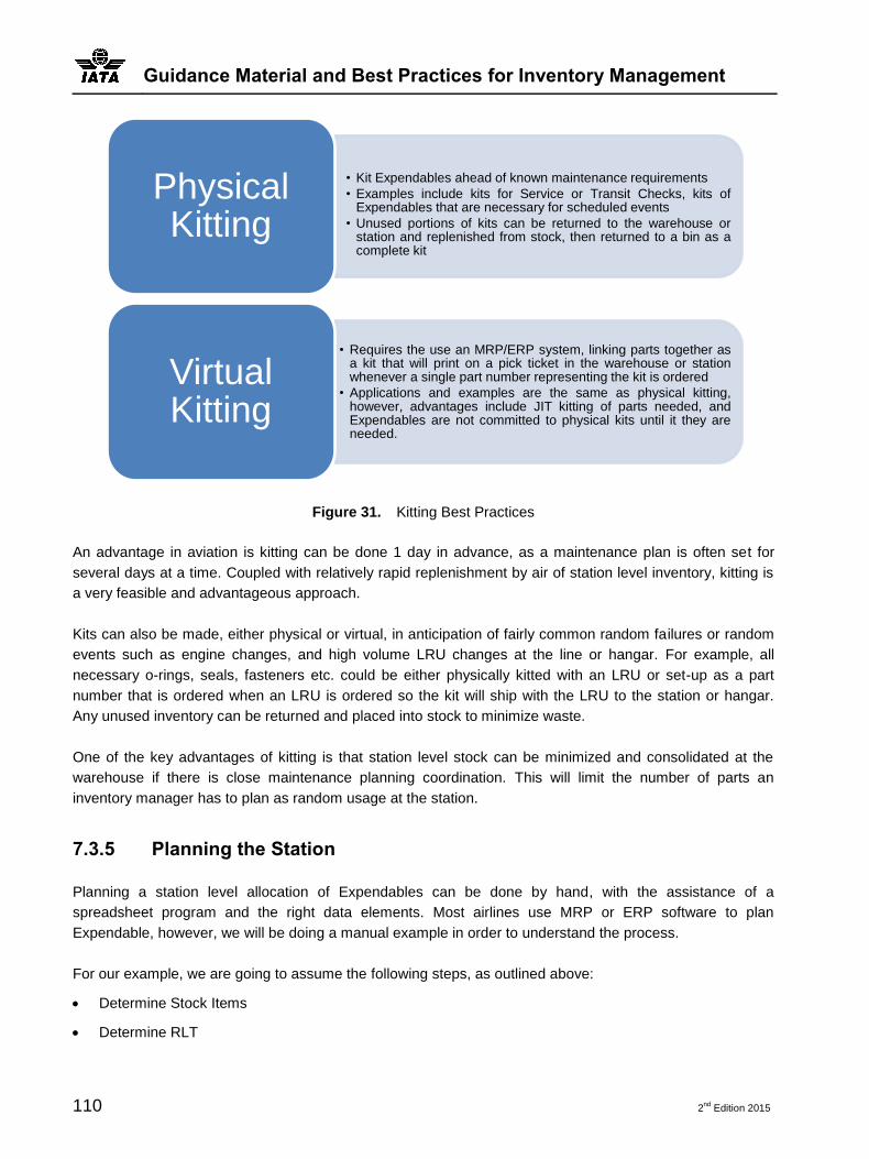
Guidance Material and Best Practices for Inventory Management
110 2nd
Edition 2015
Figure 31. Kitting Best Practices
An advantage in aviation is kitting can be done 1 day in advance, as a maintenance plan is often set for
several days at a time. Coupled with relatively rapid replenishment by air of station level inventory, kitting is
a very feasible and advantageous approach.
Kits can also be made, either physical or virtual, in anticipation of fairly common random failures or random
events such as engine changes, and high volume LRU changes at the line or hangar. For example, all
necessary o-rings, seals, fasteners etc. could be either physically kitted with an LRU or set-up as a part
number that is ordered when an LRU is ordered so the kit will ship with the LRU to the station or hangar.
Any unused inventory can be returned and placed into stock to minimize waste.
One of the key advantages of kitting is that station level stock can be minimized and consolidated at the
warehouse if there is close maintenance planning coordination. This will limit the number of parts an
inventory manager has to plan as random usage at the station.
7.3.5 Planning the Station
Planning a station level allocation of Expendables can be done by hand, with the assistance of a
spreadsheet program and the right data elements. Most airlines use MRP or ERP software to plan
Expendable, however, we will be doing a manual example in order to understand the process.
For our example, we are going to assume the following steps, as outlined above:
Determine Stock Items
Determine RLT
• Kit Expendables ahead of known maintenance requirements
• Examples include kits for Service or Transit Checks, kits of Expendables that are necessary for scheduled events
• Unused portions of kits can be returned to the warehouse or station and replenished from stock, then returned to a bin as a complete kit
Physical Kitting
• Requires the use an MRP/ERP system, linking parts together as a kit that will print on a pick ticket in the warehouse or station whenever a single part number representing the kit is ordered
• Applications and examples are the same as physical kitting, however, advantages include JIT kitting of parts needed, and Expendables are not committed to physical kits until it they are needed.
Virtual Kitting

Optimization of Airline Inventory
2nd
Edition 2015 111
Set Allocation Quantity
Set Safety Stock or Min
Determine Reorder Point and Reorder Quantity
7.3.5.1 Determine Stock Items
There may be multiple sources for determining the items to stock however the aircraft manufacturer will
provide some guidance as to which Expendables should be stocked. For a new operator, or a new fleet to
an existing operator, this is likely the only feasible starting point.
A new fleet can be modelled to an existing fleet if there is commonality between the fleets. For example
B737-800 and B737-900 are similar enough from an Expendables perspective, the main difference being
fuselage length, and Maximum Take-Off Weight (MTOW), requiring different landing gear, and perhaps
associated parts.
If an operator has a history of ordering Expendables, this may be used as well to designate stock items. Any
item with repeat orders might be considered for handling as a stock item. Infrequently used items can be
held at the warehouse, commonly used items should be forward stocked at the stations. As general
guidance consult the chart below:
Criticality Consumption Recommendation
Grounding Item (Cat 1)
And 1 usage per year or more
And Greater than instant lead time
Stock Item
Non-Grounding item
And 1 usage per year or more
And Greater than instant lead time
Stock Item
Grounding Item (Cat 1)
And Between 0.5 and 1 usage per year
And Greater than instant lead time
Stock Item, consider a warehouse only
Grounding Item With MEL relief
And Between 0.5 and 1 usage per year
And Greater than instant lead time, but within MEL relief window
Non-Stock
Non-Grounding item
And Less than 1 usage per year
And Greater than instant lead time
Non-Stock
Grounding Item With MEL relief
And Between 0.5 and 1 usage per year
And Lead time Greater than MEL relief window
Stock Item, consider a warehouse only
Table 25. Stocking Matrix-Guidance for setting items as Stock or Non-Stock

Guidance Material and Best Practices for Inventory Management
112 2nd
Edition 2015
7.3.5.2 Determine Replenishment Lead Time
RLT will often come directly from the manufacturer or distributor when planning the warehouse, however in
the case of a station we are going to assume that the warehouse has the item in stock if it is a stock item at
stations, and we have complete access to the airlines’ own network of flights. For these reasons we will
assume an RLT of 1 day.
7.3.5.3 Set Allocation Quantity
For allocation quantity, let’s assume we have 5 part numbers and we were able to find the annual demand
at the station level:
Part Number Description Annual Usage
123-1 o-ring 105
234-1 seal 184
345-1 filter 199
456-1 fastener 39
567-1 gasket 72
Further, we take the annual demand, and divide all by 365 for a daily demand quantity:
Part Number Description Annual Usage Daily Demand (DD)
123-1 o-ring 105 0.287671233
234-1 seal 184 0.504109589
345-1 filter 199 0.545205479
456-1 fastener 39 0.106849315
567-1 gasket 72 0.197260274
Notice all the daily demands are a fractional less than 1. We will need to round up. Since inventory cannot
be provided in fractional quantities, we round up to the nearest whole number.
Part Number Description Annual Usage Daily Demand (DD) Rounded DD
123-1 o-ring 105 0.287671233 1
234-1 seal 184 0.504109589 1
345-1 filter 199 0.545205479 1
456-1 fastener 39 0.106849315 1
567-1 gasket 72 0.197260274 1
We also consult with the line maintenance manager and find that there are some intermittent demand
patterns for some of the parts. Meaning, while for example the filter shows 199 used in the station during the
year, with a daily demand less than 1, there can be as many as 4 used in any given day. As such, we
update our table accordingly from our interview with maintenance:

Optimization of Airline Inventory
2nd
Edition 2015 113
Part Number Description Annual Usage Daily Demand (DD) Rounded DD Daily Max
123-1 o-ring 105 0.287671233 1 1
234-1 seal 184 0.504109589 1 2
345-1 filter 199 0.545205479 1 4
456-1 fastener 39 0.106849315 1 25
567-1 gasket 72 0.197260274 1 2
To arrive at our recommended stock quantity, we take the maximum of the Rounded DD and the Daily Max
provided by Line Maintenance:
Part Number Description Annual Usage
Daily Demand (DD)
Rounded DD Daily Max Allocation Qty
123-1 o-ring 105 0.287671233 1 1 1
234-1 seal 184 0.504109589 1 2 2
345-1 filter 199 0.545205479 1 4 4
456-1 fastener 39 0.106849315 1 25 25
567-1 gasket 72 0.197260274 1 2 2
Notice, that in all but one case (the o-ring), Maintenance guidance overrides the daily demand calculation. It
is very important to understand the demand patterns at the station being allocated. From a practical
standpoint, it does not make sense to allocate items that cannot be used by maintenance because their
allocation quantity is less than the quantity needed when used. Note that these demand patterns are caused
either by the random nature of failures or the vagaries of the flight schedule driving service check and transit
check activities, or other scheduled maintenance.
Note also we are using a daily replenishment of the station. As such, safety stock is almost inherently
included in our demand numbers since we consulted with Line Maintenance.
7.3.5.4 Set Safety Stock or Min
As stated above, we are using a daily replenishment strategy. For that reason, our safety stock
requirements will not vary greatly from our actual allocations at the station level.
Because we are using a Min/Max strategy with maintenance input, and we have a 1 day RLT from the
warehouse to the station, and we use the warehouse to absorb any undue system variation, we do not need
to set a safety stock different than a Min for the station. Furthermore, our Min represents our re-order point.
Safety Stock will be discussed in more depth in the warehouse planning example.
7.3.5.5 Determine Reorder Point
The reorder point is very much tied in with the safety stock or minimum stock level. The minimum stock level
can determine at what point the reordering is done. Once a certain part has reached a certain level of
quantity then reorder is required. The reordering can also be set at a certain time interval. A part may be

Guidance Material and Best Practices for Inventory Management
114 2nd
Edition 2015
ordered every other week, month etc. depending on the usage. The vulnerability with this method is that if
there is no minimum stock quantity set it can lead to nil stock.
Our last calculation considerations for the station are the re-order point and re-order quantity.
Reorder point represents the trigger for a replenishment order to the warehouse from the station. We will
use the Daily Max as the re-order point.
Our goal is to ensure in our model that maintenance has adequate inventory at the point of use (the station)
to accomplish maintenance. Since we are planning for random events, we will take a risk in inventory
efficiency at the station level in order to maximize maintenance opportunities. Conversely, we will plan our
warehouse very rigorously in order to take economies of scale at the warehouse level, offsetting the
inventory inefficiencies we are assuming at the station level.
Re-order quantity represents the amount ordered to bring the bin up to the daily max as designated by
maintenance.
Consider the following daily cycle:
Figure 32. Inventory and Maintenance Daily Cycle
Maintenance Plan is set
before Evening
Daily replenishments ship from warehouse to stations
Distributed Rotables and Expendable kits ship before
last flight of day from warehouse
Station receives and places
inventory into stock Station pulls
inventory needed for
nightly maintenance
Maintenance occurs overnight,
consuming inventory
Station material manager / supervisor asseses inventory
levels post-maintenance
Station orders inventory replenishment in early
morning
Warehouse pulls and preps next day's inventory
shipments

Optimization of Airline Inventory
2nd
Edition 2015 115
Note we are assuming less than 24 hours between a consumption and replenishment from the warehouse
as a best practice. In setting up the warehouse and replenishment strategy, in order to minimize stock outs
at the point of use, close daily coordination between stations and the warehouse are a necessity. Any
excess inventory is held at the warehouse and distributed in 24 hour cycles, taking advantage of the natural
logistics of airline operations. As such, the inventory reorder point and reorder quantity is processed every
24 hours.
To continue our example, we will set the re-order point as follows:
Part Number Description Rounded DD Daily Max Allocation Qty Reorder Point
123-1 o-ring 1 1 1 0
234-1 seal 1 2 2 1
345-1 filter 1 4 4 3
456-1 fastener 1 25 25 24
567-1 gasket 1 2 2 1
Note that re-order point is generally kicked off in an MRP or similar computer system, but in a small station,
could be managed using spreadsheet, although this is not recommended. Most airlines will be using some
sort of system to manage inventory quantities. Note that re-order point is set so that any time the inventory
quantity falls below the allocation quantity or “min” we will submit an order for additional materials.
Our re-order quantity will mirror nightly usage since we are on a 1 day replenishment cycle.
Part Number
Description Rounded DD
Daily Max
Allocation Qty
Reorder Point
Usage on Night x
Qty On-Hand Post Maintenance
Re-Order Qty
123-1 o-ring 1 1 1 0 0 1 0
234-1 seal 1 2 2 1 2 0 2
345-1 filter 1 4 4 3 2 2 2
456-1 fastener 1 25 25 24 15 10 15
567-1 gasket 1 2 2 1 0 2 0
For initial allocation, it may be infeasible to ship all inventory by air. This may be the case when initially
setting up a new station or when significantly de-allocating and re-allocating a station due to major schedule
change impacts to fleets, frequencies, or maintenance needs.
7.3.6 Planning the Warehouse
Warehouse planning is not unlike station planning, with the exception of certain items might be stocked at
the warehouse that are not stocked in stations, and that the safety stock and RLT is treated more rigorously
at the warehouse. Also, lot sizes may come into play.

Guidance Material and Best Practices for Inventory Management
116 2nd
Edition 2015
7.3.6.1 Minimum Lot Sizes
For example, many items are shipped from the OEM or distributor in minimum quantities. Hardware such as
fasteners may be shipped by weight. Thus while 25 fasteners might be the stocking quantity in our station
example, the warehouse may be required to order hundreds or thousands at the time by weight.
The inventory manager should assess whether the cost of breaking packages at the warehouse is
worthwhile, or should the minimum lot quantity be passed on to each station. This will be a case by case
analysis that accounts for annual usage at the station, the excess inventory that may result at the station,
balanced with the cost to break packages at the warehouse. In general, due to the high cost of most aviation
materials, breaking lots at the warehouse would be best practice.
7.3.6.2 Basic Inventory Model
We will assume a time-tested inventory model wherein the warehouse carries a certain average stock,
replenishes to a maximum, and carries a safety stock for demand side variation. We will assume a constant
lead time for replenishment from the OEM or distributor.
Figure 33. Inventory Model for Expendables
We will use this model while considering our warehouse planning design. Note that real consumption may
not follow such a clean pattern as above, however, our design of safety stock will absorb demand variation
at the warehouse, allowing us to keep a high service level at the station and bay level.

Optimization of Airline Inventory
2nd
Edition 2015 117
Figure 34. Actual Demand Pattern
Notice that in reality in the figure above, during the first period our inventory consumption dips into the safety
stock, and lead time is a little longer than expected. Our first period demand pattern, represented by the
black line, was as expected, but our replenishment came a little later than expected. In the second period,
our demand pattern was more aggressive (steeper), however our lead time was less and replenishment
came early, and we never reached safety stock levels. In the third period, demand was less aggressive than
expected, and the result is excess inventory in the third period.
7.3.6.3 Safety Stock at the Warehouse
Remember that in setting up the station, we will be depending on the warehouse to absorb variation. This
requires an approach that is a little different than station treatment, and we will plan the safety stock and re-
order points in more detail than at the station level to ensure an optimal result.
We have already determined that we have some advantages in aviation:
We have near instantaneous ability to replenish our point of use (the stations).
The warehouse can aggregate the demand of the many stations.
Our station re-order points are almost always equal to our 24 hour consumption since we have a 1 day /
24 hour RLT.
If we happen to guess wrong on stocking quantities, we can adjust forecasts, and burn down excess
Expendable inventory (this is not an option with Rotables, except in the case of scrap).
However, now as we consider the warehouse, we need to make sure that our station model will be practical
by rigorously planning the warehouse. In part this requires a focus on safety stock, or better said, on
minimizing stock outs at the station by ensuring that the warehouse is in a position to always replenish the

Guidance Material and Best Practices for Inventory Management
118 2nd
Edition 2015
stations within 24 hours. Warehouse safety stock will depend on the RLT from an OEM or distributor, which
will almost always be greater than 1 day. In fact, typical RLT’s for warehouse stock will be between 30 and
120 days, with some extending 6 months to 1 year.
Setting up the warehouse, we can use the same 5 steps as described above that we used on the station,
but we will treat safety stock and re-order points in more depth.
7.3.6.4 Calculating the Safety Stock and Reorder Points at the Warehouse
We will assume that there is a desired service level at the warehouse. This will range usually above 90%. In
other words, a service level of 90% indicates that 9 times out of ten, we avoid a stock out on an order.
Note that most warehouse service levels will exceed 95%, and approach 100% but will never be 100%.
We will express in our example service level as a probability between 0 and 1:
( )
We will also assume that any forecast error will be normally distributed with a mean of zero, and a standard
deviation of 1, via the Central Limit Theorem.42
As such, a table of values can be derived from the cumulative standard normal distribution function of the
Normal Distribution:
Service Level Probability Service Factor
90% 0.9 1.28
95% 0.95 1.64
99.7% 0.997 2.75
The service factor can be calculated in Excel using the NORMSINV function. The format for the equation in
Excel is:
( )
For where cell is any data between 0 and 1. For example:
( )
Will return a value of 1.28
42 The Central Limit Theorem (CLT) implies that the sum of n independently distributed random variables is approximately Normal
distributed N (0, 1), regardless of the distributions of the individual variables. [Montgomery, Introduction to Statistical Process Control, p.46]. See any text on statistics for a discussion of the CLT.

Optimization of Airline Inventory
2nd
Edition 2015 119
Readers familiar with statistics can look up the service factors by utilizing a table of the CDF of the standard
normal distribution, and choose any service level, and find the corresponding service factor.
We will use the service factor, implying a corresponding service level when calculating safety stock as
follows:
Where SS is Safety Stock, σ is standard deviation, and SF is the Service Factor either from the table above,
calculated with the NORMSINV Excel function, or looked up in the standard normal CDF tables in a
statistical reference (often referred to as z-tables).
LTF is Lead Time Factor. It is defined as:
√
We will always be expressing our Lead Time in days i.e. 30 days, 15 days, 120 days. Our forecast period is
1 day-we are looking at daily usage and the standard deviation around those days.
Common LTF values for our calculations will be:
Lead Time (in days) LTF
15 3.87
30 5.48
45 6.71
60 7.75
120 10.95
240 15.49
365 19.10
Assume the MRP system has captured average daily demand on a monthly basis. From this we estimate
the standard deviation of average daily demand for o-rings:
Month 1 2 3 4 5 6 7 8 9 10 12
Average Daily Demand 179 198 122 147 197 148 179 178 165 145 170
Standard Dev. 23.5
Very Important Note: We are always looking at an average daily demand, and as such we are always
looking at a daily average demand standard deviation as well. If the inventory manager uses demand
standard deviation from any other period (i.e. monthly, annual, weekly, etc.), the Safety Stock formula above
may not estimate the needed safety stock value properly. Always convert demand into daily demand. If not,
the LTF will need to be recalculated and calibrated to the forecast period.

Guidance Material and Best Practices for Inventory Management
120 2nd
Edition 2015
So, for the same 5 parts as in the station example, we have calculated an annual demand and converted
that to a DD figure. We also have the RLT from the manufacturer or distributor of each part.
Part Number Description Annual Usage Daily Demand (DD) RLT
123-1 o-ring 59917 164.2 30
234-1 seal 27538 75.4 30
345-1 filter 53945 147.8 60
456-1 fastener 69999 191.8 30
567-1 gasket 34731 95.2 120
The main differences between our warehouse model set-up and the station is we are aggregating all
demand for the system at our single warehouse, and looking at the actual lead times for replenishment
rather than the 1 day RLT used at the station level.
Our next step is to calculate Lead Time Demand:
Part Number Description Annual Usage Daily Demand (DD) RLT LT Demand
123-1 o-ring 59917 164.2 30 4924.7
234-1 seal 27538 75.4 30 2263.4
345-1 filter 53945 147.8 60 8867.7
456-1 fastener 69999 191.8 30 5753.3
567-1 gasket 34731 95.2 120 11418.4
Following this we select a service factor. For simplicity we will use 90%. We can look up in our table above,
calculate via the NORMSINV function in Excel, or look up in a statistical reference to determine that a 90%
service level generates a 1.28 Service Factor (SF).
Part Number Description Annual Usage Daily Demand (DD) RLT LT Demand Service Factor
123-1 o-ring 59917 164.2 30 4924.7 1.28
234-1 seal 27538 75.4 30 2263.4 1.28
345-1 filter 53945 147.8 60 8867.7 1.28
456-1 fastener 69999 191.8 30 5753.3 1.28
567-1 gasket 34731 95.2 120 11418.4 1.28
Note that in practice, critical items might receive a higher service factor than 90% and other less critical
items might be given a service level less than 90% to minimize cost.
We have already shown above calculation of standard deviation, σ, as well as calculating LTF, Lead Time
Factor. We do so for each part, noting that some will have different lead times than others, and of course,
varying standard deviations in demand.
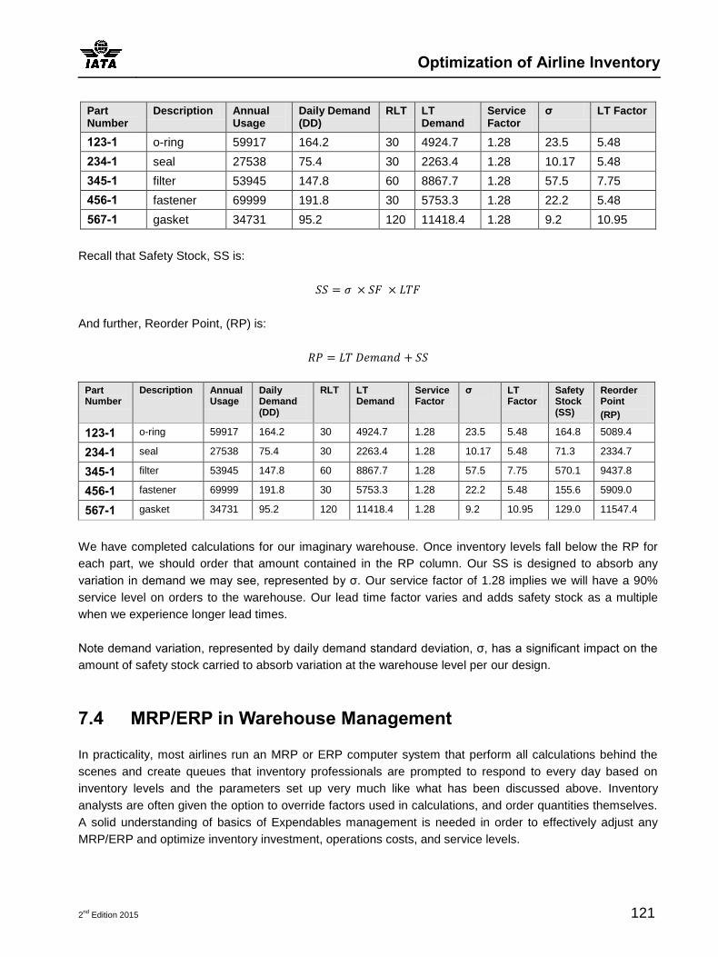
Optimization of Airline Inventory
2nd
Edition 2015 121
Part Number
Description Annual Usage
Daily Demand (DD)
RLT LT Demand
Service Factor
σ LT Factor
123-1 o-ring 59917 164.2 30 4924.7 1.28 23.5 5.48
234-1 seal 27538 75.4 30 2263.4 1.28 10.17 5.48
345-1 filter 53945 147.8 60 8867.7 1.28 57.5 7.75
456-1 fastener 69999 191.8 30 5753.3 1.28 22.2 5.48
567-1 gasket 34731 95.2 120 11418.4 1.28 9.2 10.95
Recall that Safety Stock, SS is:
And further, Reorder Point, (RP) is:
Part Number
Description Annual Usage
Daily Demand (DD)
RLT LT Demand
Service Factor
σ LT Factor
Safety Stock (SS)
Reorder Point
(RP)
123-1 o-ring 59917 164.2 30 4924.7 1.28 23.5 5.48 164.8 5089.4
234-1 seal 27538 75.4 30 2263.4 1.28 10.17 5.48 71.3 2334.7
345-1 filter 53945 147.8 60 8867.7 1.28 57.5 7.75 570.1 9437.8
456-1 fastener 69999 191.8 30 5753.3 1.28 22.2 5.48 155.6 5909.0
567-1 gasket 34731 95.2 120 11418.4 1.28 9.2 10.95 129.0 11547.4
We have completed calculations for our imaginary warehouse. Once inventory levels fall below the RP for
each part, we should order that amount contained in the RP column. Our SS is designed to absorb any
variation in demand we may see, represented by σ. Our service factor of 1.28 implies we will have a 90%
service level on orders to the warehouse. Our lead time factor varies and adds safety stock as a multiple
when we experience longer lead times.
Note demand variation, represented by daily demand standard deviation, σ, has a significant impact on the
amount of safety stock carried to absorb variation at the warehouse level per our design.
7.4 MRP/ERP in Warehouse Management
In practicality, most airlines run an MRP or ERP computer system that perform all calculations behind the
scenes and create queues that inventory professionals are prompted to respond to every day based on
inventory levels and the parameters set up very much like what has been discussed above. Inventory
analysts are often given the option to override factors used in calculations, and order quantities themselves.
A solid understanding of basics of Expendables management is needed in order to effectively adjust any
MRP/ERP and optimize inventory investment, operations costs, and service levels.

Guidance Material and Best Practices for Inventory Management
122 2nd
Edition 2015
7.4.1 EOQ in Warehouse Management
Economic Order Quantity is a time-tested formula for minimizing total cost of inventory. While not
recommended at an airline station or bay level, it does make sense to explore at the warehouse level.
In the warehouse example above, we use the RP quantity as our order quantity for replenishment. However,
once shipping and other costs come into play, as well as the cost of carrying inventory, an inventory
manager will want a method to minimize total cost of ownership over time. EOQ provides a method to
optimize costs or ordering versus cost of carrying excess inventory.
EOQ literature is widespread, detailing development of the formula as well as pros and cons. Refer to any
commonly available source for further depth.
For our purpose, we will use EOQ and compare to the RP calculated above.
Note that the basic EOQ formula is as follows:
√
From our previous work, we are aware of annual demand.
Order cost represents all the cost and activity associated with a single order: shipping if not included in a
cost per unit, costs to process an order, costs to receive an order at the warehouse, receiving inspection,
etc. This would be a static cost per order.
Holding cost is a percentage often in the 4-15% range. It includes the cost of money (cash tied up in
inventory rather than other investments), pilferage/loss, insurance costs, etc.
Unit cost is the price per unit. Note that our EOQ formula does not allow for volume discounts. Methods
have been researched which do allow for adding volume discount, but the math can become cumbersome.
An inventory manager can adopt a more complex method of EOQ, or run several scenarios easily in Excel
or a similar spreadsheet to determine the EOQ with volume discounts.
For our five previous example parts, we will assume we calculated the RP (Re-order Point) as before and
will compare to the EOQ to see if we can further optimize inventory costs.
For our O-ring, we deduce an order cost of $120, a cost per unit of $1.25, and an inventory holding cost
percentage provided to us by Finance of 7.5%, and our annual demand was 59,917 units:
√

Optimization of Airline Inventory
2nd
Edition 2015 123
√
We can run the calculation for all our 5 example parts, assuming the annual demand previously provided,
the same Holding Cost %, variable cost per unit, and variable order cost by part:
Part Number
Description Annual Usage
Order Cost Cost Per Unit
Holding Cost %
EOQ
123-1 o-ring 59917 $ 120 $ 1.25 7.50% 12,385
234-1 seal 27538 $ 60 $ 5.60 7.50% 2,805
345-1 Filter 53945 $ 500 $ 550.75 7.50% 1,143
456-1 Fastener 69999 $ 350 $ 5.35 7.50% 11,051
567-1 Gasket 34731 $ 120 $ 25.60 7.50% 2,084
Comparison of the RP to EOQ quantities yield some interesting observations:
Part Number
Description Reorder Point
EOQ Max EOQ or RP
Source EOQ Orders Per Year
RP Order Per Year
123-1 o-ring 5089.4 12,385 12,385 EOQ 5 12
234-1 seal 2334.7 2,805 2,805 EOQ 10 12
345-1 filter 9437.8 1,143 9,438 RP 48 6
456-1 fastener 5909.0 11,051 11,051 EOQ 7 12
567-1 gasket 11547.4 2,084 11,547 RP 17 4
TOTAL 87 46
Not surprisingly, more orders per year are generated in total with EOQ: 87 for EOQ versus 46 for the RP
method. This is to be expected since the RP method is only demand related, while the EOQ takes into
consideration the total cost of ownership.
In the case of the filter, with a high part cost, and high ordering cost, EOQ drives 48 orders per year versus
the 6 indicated by the RP method. In layman’s terms, this high dollar Expendable is ordered nearly every
week to keep up with consumption. As the order cost decreases, the expected number of orders per year
will increase.
7.4.2 Discussion of Ordering Strategies
Paramount for the inventory manager is to avoid stock outs, however, in the extreme, carrying a year’s
worth of inventory exposes many types of risk: increased obsolescence as part numbers change, high
inventory carrying costs as the warehouse is stocked with a glut of inventory for all parts. EOQ can help
balance the cost to order versus cost to carry.

Guidance Material and Best Practices for Inventory Management
124 2nd
Edition 2015
Frequent ordering will drive a higher transactional cost (i.e. analyst time), but modern ERP/MRP systems
mitigate the amount of time that must be spent per order.
Some MRP/ERP software programs offer auto-replenishment to offset the increased number of orders
driven by EOQ in an effort to minimize total cost of inventory. However, care should be taken in adopting a
completely automatic ordering environment as runaway stock levels can occur quickly, and forecast
adjustments (either increase in usage or decrease in usage) might not be caught in time.
The inventory manager will need to carefully determine which items might be candidates for auto-
replenishment, and which deserve complete analyst scrutiny at every order.
Categorizing inventory via the A-B-C method may provide insight to the inventory manager for how to
handle Expendable management.
Briefly, the concept of ABC inventory has been in use for some time. Many inventory management and
supply chain texts and resources detail this method. Warehouse have been organized for decades affording
easy access to fast-moving A items, and placing the C-items in the less optimal locations for retrieval since
the need is intermittent.
A-Items are those defined as high use in the system. C-Items are defined as slow moving items. B-items are
all other items that are neither A or C item.
In aviation for Expendables, the same concept can be applied in setting up the line stockroom, hangar floor
stock, warehouse, as well as the planning function.
For general guidance, consider the following chart:
Classification Description Recommended Metrics
A-Items
Fast moving inventory consumed daily, weekly or monthly, may have intermittent demand patterns.
Inventory Turns > 5.0
B-Items
Slower moving than A-items, and may have intermittent or very seasonal demand (e.g. high summer usage). More likely to be seasonal and intermittent than A-items.
Inventory Turns Between 1.0 and 5.0
C-Items Slow moving items. Inventory Turns < 1.0
Table 26. Classification of Expendable Material
An inventory manager may want to adjust the recommended turn metrics and also create a list of critical
parts (No-Go, MEL) versus normal use parts.
Any critical part may be flagged to always be in an analysts queue for review. In addition, any long lead time
items (>60 days) may need to be flagged for constant review as well.

Optimization of Airline Inventory
2nd
Edition 2015 125
7.4.2.1 Planning for the Hangar Bay
Hangar operations differ from line operations in that the cycle is typically longer-30 days or more for a C or D
Check, and smaller visits that may be as short as a few days. There may also be aircraft modifications or
other activities that fall between a 5 and 30 day window of typical heavy maintenance visits, an example
being a cabin refurbishment that may be accomplished in just a few days. Contrasted with the daily cycle of
live flight line maintenance and nightly line maintenance activities, the hangar bay seems to have a luxury of
time. However, a stock out in the hangar can be just as critical as on the line.
Consider also that for many airlines that still perform their own heavy maintenance, the hangar and
materials warehouse are usually co-located.
It is recommended to think of the hangar bay or bays as a line station, with a 24-hour (or shorter)
replenishment cycle from the warehouse. It is generally easier to logistically service the hangar versus a line
station since the hangar does not depend on flight operations to deliver needed parts. Forward stocked
commonly used items can be set-up on the hangar floor as floor stock and expensed at the time of issue,
and quantities monitored for replenishment by a stock clerk, or by other inventory control methods (bar
coding to a work order for example). Special or large items can always be ordered from the warehouse.
Kitting, as discussed above is also a good option for hangar operations. Finally consumables such as
gloves, sealants, etc. can be treated just as Expendables, and may be managed in any myriad of ways
appropriate for Expendables as they share the same inventory characteristics.
Further, since the hangar work is composed of a large majority of routine jobs known in advance, the entire
complement of parts needed to accomplish all maintenance activities for the visit can be pre-drawn and
delivered to the bay as the aircraft arrives (or at least along the critical path of the aircraft visit). Kitting of
Expendables with Rotables to be changed for time control will minimize the need to order parts by
mechanics. Unused parts can be either absorbed into floor stock, or returned to the warehouse post-visit. A
complement of Expendables needed for non-routine jobs can be developed statistically from known past
non-routine activity. Again, any unused parts could be then returned to the warehouse, or absorbed into
floor stock.
7.4.2.2 Control of Expendable Inventories
As noted in the accounting section later, Expendables are expensed at the time of issue. Usually they are
expensed to a department, and not necessarily to an aircraft number at most airlines. For example, line
maintenance will have an expense budget for a fiscal year, and any Expendable use will be against that
budget.
Usually the inventory manager will partner with accounting in order to determine the most appropriate
method of accounting and Expendable control.

Guidance Material and Best Practices for Inventory Management
126 2nd
Edition 2015
In the hangar, there may be an organizational desire to account for all Expendable use against a job which
will track to an aircraft. Any Expendables issued from the warehouse to the hangar will be expensed against
the applicable job number.
7.4.2.3 Inventory Accuracy
Inventory accuracy is important for a number of reasons, not the least of which being that many airlines are
publicly traded and the inventory valuation is an important aspect to the balance sheet. Write-ups and write-
downs of inventory have undesirable consequences.
However, in a more practical sense, inventory accuracy is paramount to the planning regimen discussed in
this entire section, as many of the assumptions are based on the premise that the inventory is actually there.
There are many resources online, and in print discussing the merits of physical inventory and cycle
counting. Suffice it to say that in the line station, cycle counting during the off-peak hours, planned so that
the entire station is counted perhaps monthly to quarterly is a recommended approach. Planning inventory
or maintenance will be impossible without a level of confidence in the actual inventory levels in the station.
Since many airlines expense at the time of issue, and lose system visibility to the actual bin levels at a
station, it is paramount to understand that the underlying assumptions of the planning function rely on
accurate controls at the station level.
In the warehouse, cycle counting is also recommended to maintain accuracy. Many long lead time items and
critical items stored in the warehouse must be accurately reflected in quantities.
2nd
Edition 2015 127
Section 8—Accounting for Rotables and Expendables
8.1 Introduction
This section is meant to be a brief discussion of typical accounting treatments of aircraft materials in an
airline and is not intended to be a complete and authoritative treatise on accounting rules worldwide.
Rather the intent of this section is based on common accounting business practices as they relate to
aviation inventory and maintenance operations.
8.2 Rotables
Rotables, as previously discussed are aircraft parts that are purchased, placed into inventory as assets, and
persist in the inventory system until scrap.
Some key characteristics of Rotable inventory:
Are treated as assets on the balance sheet of a company.
Have a repair process per a maintenance manual and can undergo from one to many repairs or
overhauls during its lifespan.
Can have a scrap threshold set by accounting which triggers the scrap process. An example being 60%
of CLP, although these percentages vary widely or it can be determined by the FMV of the part and
decided by the purchasing or repair department.
Have a scrap rate, usually very low, but certainly less than 100%.
May have a lifetime of 5 to 25 years or more, depending on the depreciation schedule used by the
company’s accounting department.
Accumulates depreciation expense to a residual value during their lifetime.
Have a residual value at scrap or end of their useful life.
Must be scrapped or designated surplus in order to be written off as an expense at the end of useful life.
Accounting generally treats Rotables as assets. In many accounting systems there will be an asset record
which records the value of the Rotable at purchase. There may be lots/groups of asset records if several
were purchased at the same time, facilitating the depreciation process for accounting.
Residual values are set by accounting, but are often in the 20% range. Note that this value is often too high,
as discussed on other sections throughout this book, since an airline will not realize 20% recovery of the
value of a Rotable at the end of its useful life. Rather, pennies on the dollar are typically realized. This often

Guidance Material and Best Practices for Inventory Management
128 2nd
Edition 2015
results in large write downs of inventory when surplus or scrap activities occur. It is recommended that an
airline study its own Rotable scrap and surplus sales and set a residual value accordingly.
Scrapping Rotables usually requires an expense to be written to a certain department. In airlines that
maintain repair capabilities this will be the repair shop. In airlines that maintain 100% outside repair, the
expense may be written to either the inventory planning/management function, or alternatively to the outside
repair department, depending on organizational objectives around scrap. Since the outside repair function
typically reviews and approves repairs by vendors, it is recommended that the scrap expense be charged to
the outside repair department in these situations.
Surplus of excess Rotables is often used to generate cash and move non-liquid assets from the balance
sheet. Examples include fleet retirement generating the need to surplus excess stock no longer needed and
not effective on remaining fleets.
Write-downs for scrap and surplus are often done on a First In First Out (FIFO) method as the asset record
is not usually tied to a serialized asset. In other words, the oldest, most depreciated asset is usually chosen
by accounting in order to minimize the write-down exposure if scrapping, or when surplus sale value is
exceeded by the remaining value of the asset.
8.3 Expendables/Consumables
Expendable and Consumable inventory differs from Rotable inventory in some key characteristics:
Expendables generally have 100% scrap rate as they are consumed at the time of use.
Expendables are usually expensed to a department or job at the time of issue.
Expendable balances are held as an asset on the balance sheet until time of issue.
Expendables are usually expensed when issued from the warehouse, but in some instances, they may
not be expensed until the point of use.
Aviation Expendables more closely fit the typical definition of inventory from an accounting perspective than
Rotables.
At a warehouse level, the Expendable balance is an asset. Once issued to a location (station, hangar bay,
shop etc.), the value of the Expendables issued is expensed against that department.
Most airlines do not track Expendable values for accounting purposes beyond the warehouse. While
MRP/ERP systems may imply or carry quantities on hand for management and planning purposes, financial
transactions in the expense process have already handled the value of the Expendables at the interface
between warehouse and issuance to a location.
Only in rare cases, such as in some hangar environments, very high dollar Expendable items, or an MRO
shop do Expendables get expensed to a job or an aircraft.

Accounting for Rotables and Expendables
2nd
Edition 2015 129
In some cases, if an aircraft modification is to be capitalized, and thus increase the book value of the
aircraft, Expendables may be included in the modification cost that is capitalized.
In some cases where an airline issues to a station, but does not expense at the time of issue, that station is
then known as an accountable station. This may be done in the case of a large station that is a mid-tier
supplier to satellite stations. Consider the graphic below:
Figure 35. Accountable and Non-Accountable Stations
Any issue from Warehouse to Station xyz will not be expensed. Any issue from the Warehouse to Station
ghi will be expensed.
Station xyz expenses any issue to Stations abc or def.
There are advantages and disadvantages to such as system. Station xyz functions as a mini-warehouse,
supplying Expendables as needed to satellite stations. This may be done in a network that does not allow
advantageous flights directly from the warehouse location to the stations. Station xyz will, by nature, require
greater inventory accuracy than satellite stations, since orders from Stations abc and def will be replenished
from Station xyz stock. Station xyz will require more rigorous control of inventory quantities, perhaps
requiring a more aggressive inventory counting plan (physical inventories versus periodic cycle counting).
Also, an inventory manager might consider whether Station xyz can order directly from OEM or distributor to
replenish stock.
Finally, issues within station to maintenance for accountable Station xyz will need to be transacted
individually to expense inventory at the time of issue. To avoid this, the additional complexity of setting up a
warehouse location and a station inventory location at the same site can be pursued. This would require
Non-Accountable
Accountable Accountable
Warehouse
Accountable Station xyz
Station abc
Station def
Station ghi

Guidance Material and Best Practices for Inventory Management
130 2nd
Edition 2015
physical separation of the inventory in Station xyz into warehouse quantities and values that are held on the
balance sheet, and station quantities and values that were expensed when issued.
In the above example, from an accounting perspective, the accountable locations will require valuation of
Expendable inventory be held on the balance sheet. Non-accountable locations are expensed at the time of
issue.
8.4 Accounting Summary
Rotables and Expendables are treated quite differently according to accounting rules, and the consideration
of these differences can affect management decisions.
An inventory manager is encouraged to partner with the finance and accounting departments for guidance in
achieving the optimal management solution for the company. It goes without saying that any treatment of
inventory should comply with all applicable laws and accounting standards.

2nd
Edition 2015 131
Section 9—New Value Chain Options
9.1 Point-of-Use Trends
Point-of-use inventory refers to materials that are made available at the work location rather than being
dependent upon ordering from a stockroom.
Point-of-use inventory has been in practice for decades in manufacturing and has in recent years begun to
penetrate aviation maintenance. Most notably, visit any MRO facility and the observer will see floor stock
available to mechanics working customer parts. In addition there may be multiple vending solutions, much
like a food or drink machine where a mechanic can draw parts very near to the workstation rather than
wasting time walking to the stock room or waiting for a delivery. The inventory items are securely stored in
the vending machine and require a bar code or ID number to draw materials from the machine.
The advantages of point of use inventory are immediately evident. Point of use inventory eliminates the
waste of excessive movement by the workforce, or the loss of time awaiting a delivery from a stock room.
Stock outs are immediately visible. If the vending machine is wired or wireless and can communicate stock
levels, on-demand replenishment from the warehouse can be accomplished.
Traditional resistance to point of use inventory has been centred around the lack of control, not only of “free
issue” inventory itself, but also the planning and replenishment. While seen as a boon to maintenance, all
other stakeholders generally would take a negative view of point of use systems. Older point of use systems
required milk-run replenishments, first to see if inventory was required and then also to re-stock. Planning
functions would often have no visibility to the inventory levels on the shop/hangar floor or line room. A stock-
out in one location might be counterbalanced with an excess in another location, but visibility to inventory
levels outside the warehouse was limited without very manual processes to stay abreast of inventory levels.
Recent penetration of technology into this space has mitigated largely the concerns of runaway inventory
and related difficulties. Barcoding coupled with vending solutions are increasingly seen on shop floors,
hangar bays and line rooms. Initially, bar coded free issue bins were somewhat commonplace, but now
vending solutions are becoming prevalent. Even wireless-connected vending is a technology today-opening
up many possibilities for inventory management.
As technology and connectivity continue to evolve, the age-old idea of point of use inventory becomes more
and more attractive for all stakeholders.
9.2 Distributive Versus Allocated Models
In past years, many airlines relied wholly on what can be termed loosely as an “Allocated Model”. Section 4
of this manual shows how one can calculate and manage quite effectively an allocated model. However,
understanding the genesis and application of “Distributed Model” may open the horizons for an inventory
manager to explore new techniques and more efficient methods for provisioning for aircraft maintenance.

Guidance Material and Best Practices for Inventory Management
132 2nd
Edition 2015
Allocated models thrived on certain assumptions and tenets for many years:
The majority of aircraft maintenance activity and this inventory use is driven by random, non-routine
events.
The randomness of aircraft maintenance requires the deployment of many materials across the network
of stations that an airline operates.
In both hub and spoke and point-to-point flight models, holding inventory at stations where it can be
used is preferred to holding inventory in the warehouse where it must be moved somewhere else when
needed before it can be used.
In the not so distant world without technology (i.e. computers), information moved via manual paperwork
(pick tickets, shortage sheets, order sheets, etc.) and hot items required labor intensive manual
processes such as phone calls.
Allocated models were cutting edge technology for many years, powered by very advanced statistical
analysis. However, at its core, an allocated model is a guess-a gamble that a part failure will occur in a
certain location. Likened to roulette, one can certainly expect to win if every red and black number is
covered with a bet, but will go absolutely broke doing so.
Recently, with the advent of ever advanced management software and the speed of information, a new
trend has been emerging: distributive models. A distributive model essentially takes all known demand and
creates a nightly/daily/weekly plan to complete the maintenance required. Inventory is distributed from a
central location to the stations that will accomplish the work using the carrier’s own flight network where
feasible. Unused and unserviceable inventory are routed back to the central warehouse for re-deployment or
induction into the repair cycle.
Distributed models have the following characteristics:
Lower overall inventory value since multiple assets need not be allocated to stations “just-in-case”.
A close tie with maintenance planning to produce a nightly distribution and maintenance plan or a
weekly hangar plan.
Recognition that all demand, even random failures, can be scheduled and thus become “known”
demand once they occur. The exceptions are the very few grounding random failures that occur during
live flight operations.
MEL relief provides a tool to manage aircraft demand and safely dispatch an aircraft requiring repair.
An integrated system that can either publish a maintenance plan and required inventory distributions, or
schedule maintenance and flights to locations with available inventory (i.e. aircraft routing has inventory
visibility).
A discipline to schedule that adheres to planning horizons and cut-offs to ensure that parts, aircraft, and
mechanics intersect at the right moment in time to accomplish the planned event.
A realization that the majority of events requiring materials are known and scheduled in advance. First
hand research by the author indicates that upwards of 80% material demand is known or can be known
in advance. Contrast this with the tenet driving allocated models that the majority of demand is random.

New Value Chain Options
2nd
Edition 2015 133
Drawing on a construct earlier in this document, we see a cycle where we can superimpose time and
support activities that might represent one daily cycle for management of a distributive model:
Figure 36. Daily Cycle of a Distributive Model
Times and activities can be adjusted but the basic premise remains the same-cooperation between
inventory planning, station material management, line maintenance and maintenance planning can result in
a more efficient distributive model.

Guidance Material and Best Practices for Inventory Management
134 2nd
Edition 2015
Section 10—Inventory Assessment
10.1 OECM
Operational Efficiency & Cost Management (OECM)43 assessment is an effort to help airlines identify and
develop cost-efficient operational solutions. The OECM assessment of airline inventory operates on the
basic principle of the airline providing the highest possible service level at the lowest total cost. Service
levels can be measured in various ways as discussed in 4.1.
When assessing the airline’s inventory management system, the OECM team hones in on the areas of cost
and also the revenue generating possibilities. Since airline inventory is very valuable and can generate cash
revenue for the airline while it is idle, the OECM team will often find a total cost offset that is a combination
of cost savings and revenue generation. Sources of cost include the cash invested to buy inventory, carrying
cost of inventory (taxes, insurance, depreciation, obsolescence, etc.), and transactional fees such as loans,
AOG expedite fees, and pooling memberships. Usually there are five key areas in a typical OECM
assessment:
Planning methodology
Engine leasing or sale
Rotable surplus
Expendable surplus
Rotable pooling
The OECM assessment evaluates the existence and function of the inventory planning functions within an
airline. At the highest level, the inventory portion of the OECM assessment is an evaluation of the efficiency
of the planning organisation in providing the highest possible service level at the lowest possible cost. The
assessment compares the airlines function versus best practises and industry benchmarks.
Typical findings in the OECM assessment:
Uncontrolled inventory purchase spends.
Transactional cost to expedite inventory that mask an inventory problem. These are in the form of loan
charges and exchange fees.
Low inventory turns on items expected to be high-turn.
Idle inventory in both Rotable and Expendables.
Surplus inventory due to:
43 www.iata.org/oecm

Inventory Assessment
2nd
Edition 2015 135
o Un-used purchases
o Automatic purchases due to scrap
o Slow increase in inventory that has accumulated over many years
o Discontinue of usage for various reason
10.2 Recommendation and Examples
10.2.1 Recommendation
Best practice among many airlines is to hold balances stable or reduce them with mature fleets whereas of
course new fleets will increase the balance.
Since the inventory balance is an aggregate number across all fleets, often increases in one fleet can be
offset by decreases in another if the airline operates a mixed fleet.
Rotable spares and Expendables should be analysed separately.
Progressive pooling and inventory exchange agreements are common in the industry. Often if an airline has
maintenance provided by an MRO, inventory support can be included. Pooling and exchange agreements
should drive the airline’s requirement for inventory down and result in a decline in balance, or can be used to
offset planned growth.
Care must be taken that new fleet addition does not result in an automatic inventory addition that may not be
needed. Any time new aircraft or new station service is introduced, the inventory management department
should analyse inventory levels using common MTBR formulas to evaluate the need for any new inventory.
Best practice is to evaluate spares formulas at every schedule change.
Inventory turns must also be analyzed on a regular basis. This analysis can occur on a part number basis in
a spreadsheet format. Inventory turn analysis should be balanced with the firms carry cost of inventory and
the cost of available means to provide a part other than ownership (i.e. borrow/exchange/pool a part rather
than own it). Any turn number that is below the firm’s target for inventory should be analyzed in depth and a
decision made as to the proper ownership strategy for that part. Special attention should be paid to parts
that are not flight critical for savings can be generated by maintaining the proper level of deferrable
inventory. This analysis may generate surplus from time to time
Inventory WIP should be closely monitored, along with the TAT for each part Rotable part. Since WIP =
Daily Demand X TAT (In days), any increase of TAT will drive the need for spares up. Further, these
additional WIP spares are of no use to the airline in daily operations because they represent unserviceable
inventory in the repair process and are not available to service aircraft on the flight line. Care should be
taken to manage WIP very closely since these spares only support the repair process. An analysis of the
ratio of the allocated value of spares to WIP spare value should be completed at least quarterly (allocated
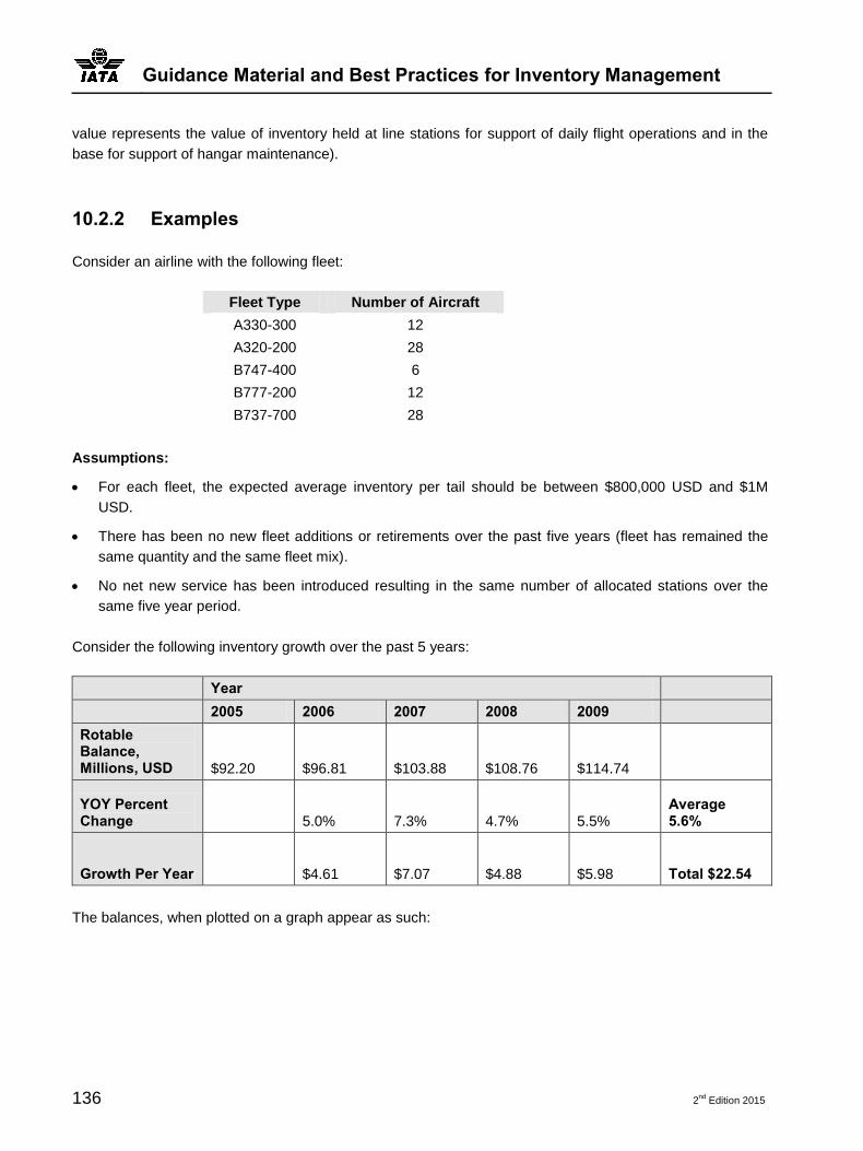
Guidance Material and Best Practices for Inventory Management
136 2nd
Edition 2015
value represents the value of inventory held at line stations for support of daily flight operations and in the
base for support of hangar maintenance).
10.2.2 Examples
Consider an airline with the following fleet:
Fleet Type Number of Aircraft
A330-300 12
A320-200 28
B747-400 6
B777-200 12
B737-700 28
Assumptions:
For each fleet, the expected average inventory per tail should be between $800,000 USD and $1M
USD.
There has been no new fleet additions or retirements over the past five years (fleet has remained the
same quantity and the same fleet mix).
No net new service has been introduced resulting in the same number of allocated stations over the
same five year period.
Consider the following inventory growth over the past 5 years:
Year
2005 2006 2007 2008 2009
Rotable Balance, Millions, USD $92.20 $96.81 $103.88 $108.76 $114.74
YOY Percent Change
5.0% 7.3% 4.7% 5.5% Average 5.6%
Growth Per Year
$4.61 $7.07 $4.88 $5.98 Total $22.54
The balances, when plotted on a graph appear as such:

Inventory Assessment
2nd
Edition 2015 137
Figure 37. Rotable Balance
We can observe from the table and the graph that the balance is growing year over year by an average of
greater than 5%. Over the five year period, the growth totals to $22.56M USD. For scale, this amount of
balance growth can be equated to between 22 and 28 new aircraft added to the fleet in terms of inventory
balance (with the assumption of inventory per tail being between $800K and $1M USD per aircraft).
If the balance in the above example is found to have no explanation, a thorough review of planning
processes and purchase controls would be in order.
$92.20
$96.81
$103.88
$108.76
$114.74
Rotable Balance, Millions, USD
2005 20062007 20082009

Guidance Material and Best Practices for Inventory Management
138 2nd
Edition 2015
Section 11—Work Cited
Boeing, Commercial Airplane Group, Customer Services Division. Spares Provisioning Products Guide,
Revision B, Document No. D6-81834. Seattle, Washington: Boeing, 1997.
Hines, William W., and Douglas C. Montgomery. Probability and Statistics in Engineering and Management
Science, Third Edition. New York: John Wiley & Sons, Inc., 1990.
Kiemele, Mark J., Stephen R. Schmidt, Berdine, and Ronald J. Basic Statistics Tools for Continouous
Improvement, 4th Edition. Colorado Springs, CO: Air Academy Press & Associates, LLC, 1999.
Montgomery, Douglas C. Introduction to Statistical Process Control, Second Edition. New York: John Wiley
& Sons, Inc., 1991.
Pande, Peter S., Robert P. Neuman, and Roland R. Cavanaugh. The Six Sigma Way: How GE, Motorola,
and other top companies are honing their performance. New York: McGraw-Hill, 2000.
Ross, Sheldon M. Introduction to Probability Model, Fourth Edition. Boston: Harcourt Brace Jovanovich,
1989.
Sherbrooke, Craig C. Optimal Inventory Modelling of Systems: Multi-Echelon Techniques. New York: John
Wiley & Sons, Inc., 1992.
Winston, Wayne L. Introduction to Mathematical Programming: Applications and Algorithms. Boston: PWS-
Kent Publishing Company, 1991.

2nd
Edition 2015 139
Section 12—Acknowledgements
Craig Wimer, Author, Wimer Aero Associates, www.wimeraero.com
Chris Markou, Editor, International Air Transport Association, www.iata.org
Elentinus Margeirsson, Editor, International Air Transport Association, www.iata.org
IATA would like to thank airlines and industry experts who reviewed this document, and provided valuable
comments.

Guidance Material and Best Practices for Inventory Management
140 2nd
Edition 2015
INTENTIONALLY LEFT BLANK

to order: www.iata.org/publishing
+1 800 716 6326
Follow us on Twitter: www.twitter.com/iata
Join us on Linkedin: www.iata.org/linkedin
Follow us on Youtube: www.youtube.com/iatatv
ISBN 978-92-9252-741-9Printed in Canada