Guarded Transition Systems: a new States/Events Formalism for ... · Boolean expressions...
21
Guarded Transition Systems: a new States/Events Formalism for Reliability Studies Antoine Rauzy IML/CNRS 169, Avenue de Luminy 13288 Marseille Cedex 9 FRANCE [email protected] Abstract: States/events formalisms, like Markov Graphs or Petri Nets, are widely used in the reliability engineering framework. They have proved to be a very powerful tool both from a conceptual and practical viewpoints. This article introduces a new states/events formalism, so called Guarded Transition Systems. Guarded Transition Systems generalize both Block Diagrams and Petri Nets. They also make it possible to handle looped systems that no existing formalism is able to handle smoothly. We illustrate their use by means of examples and discusses several important issues like composition and graphical representations. 1. Introduction Description formalisms used for risk analyses can be roughly separated into two categories: combinatorial models, like Fault Trees or Block Diagrams and states/events formalisms, like Markov Graphs or Petri Nets (see e.g. [AM93] for a general presentation). Advantages and drawbacks of each of them have been extensively discussed in the literature. The choice of a formalism results always of a trade-off. On the one hand, a modelling formalism should be as expressive as possible. On the other hand, the greater the expressive power, the lower the efficiency of associated assessment methods. There is no “silver bullet”. However, a formalism may offer or not some convenient modelling features and may exploit fully or not assessment techniques. Hence, not all of the formalisms within a category are equally suitable.
Transcript of Guarded Transition Systems: a new States/Events Formalism for ... · Boolean expressions...

Guarded Transition Systems:
a new States/Events Formalism for Reliability Studies
Antoine Rauzy
IML/CNRS
169, Avenue de Luminy
13288 Marseille Cedex 9
FRANCE
Abstract: States/events formalisms, like Markov Graphs or Petri Nets, are widely used in the
reliability engineering framework. They have proved to be a very powerful tool both from a
conceptual and practical viewpoints. This article introduces a new states/events formalism, so
called Guarded Transition Systems. Guarded Transition Systems generalize both Block
Diagrams and Petri Nets. They also make it possible to handle looped systems that no existing
formalism is able to handle smoothly. We illustrate their use by means of examples and
discusses several important issues like composition and graphical representations.
1. Introduction
Description formalisms used for risk analyses can be roughly separated into two categories:
combinatorial models, like Fault Trees or Block Diagrams and states/events formalisms, like
Markov Graphs or Petri Nets (see e.g. [AM93] for a general presentation). Advantages and
drawbacks of each of them have been extensively discussed in the literature. The choice of a
formalism results always of a trade-off. On the one hand, a modelling formalism should be as
expressive as possible. On the other hand, the greater the expressive power, the lower the
efficiency of associated assessment methods. There is no “silver bullet”. However, a
formalism may offer or not some convenient modelling features and may exploit fully or not
assessment techniques. Hence, not all of the formalisms within a category are equally suitable.

This article introduces a new states/events formalism, so called Guarded Transition Systems.
Guarded Transition Systems can be seen as a generalization of both Block Diagrams, Petri Nets
and Arnold-Nivat model of parallelism [Arn94]. From Petri nets, they take the idea of having
states represented by means of variables (places) and changes of states represented by means of
events and transitions. From, Block Diagrams, they take the notion of flow circulating through
the a network, therefore allowing the descriptions of remote interactions between components
of the system under study. From Arnold-Nivat model of parallelism, they take the notions of
composition and explicit synchronization which are a very powerful means to create
hierarchical models. The important point is that these generalizations come with no cost.
Useful assessment algorithms for Petri Nets or Finite State Machines are easily lift up to
Guarded Transition Systems without a significant change of complexity.
None of the cited formalisms (Petri Nets, Block Diagrams, Finite State Machines), is suitable to
model looped systems. A system is said looped when it embeds two components A and B such
that the state of A depends on the state of B and vice-versa. Looped systems arise typically in
reliability analyses of electrical networks. Electrical networks can be abstracted as graphs with
distinguished source and target nodes and whose nodes are subject to failures. A target node T
is powered if there exists a least one working path from one of the source nodes to T.
Intuitively, the difficulty to describe this kind of systems comes from the fact that to know
whether a target node is powered or not, we cannot just look at its adjacent nodes and edges. In
fact, there is no other solution than to propagate the states of source nodes through the network.
This propagation has to be renewed each time a node changes of state (working or failed).
With Guarded Transitions Systems, we intoduce a fixpoint calculation after each transition
firing. This fixpoint mechanism makes it possible to handle looped systems is a simple and
elegant way.
One of the main reasons of the success of the Petri Nets and Block Diagrams stands in their
graphical representation: a drawing tells us often much more than a long text. However,
graphics have their own limits: the size of the paper sheet or the computer screen. As models
get bigger, it is not possible to represent them fully within a single graphic. Rather, we should
use graphics as incomplete views of the model. Software specification languages such as UML
[RJB99] advocate that it is often much more convenient to have several partial views of the
same object than to have a single overloaded view. We discuss here how to apply this idea to
Guarded Transition Systems.
The remainder of this article is organized as follows. Section 2 presents a motivating example.
Section 3 defines Guarded Transition Systems and shows some examples of their use. Section

5 discusses the mechanisms by which Guarded Transition Systems can be composed, i.e. how
to build hierarchical and modular descriptions and compile these descriptions into Guarded
Transition Systems. Section 5 generalizes the definition of Guarded Transition Systems to
Stochastic Guarded Transition Systems. Finally, Section 6 discusses graphical representations
for Guarded Transition Systems.
2. Motivating Example
Consider the network pictured Figure 1. This network has two source nodes S1 and S2 and
seven target nodes numbered from T1 to T7. We assume that nodes are subject to failures and
can be repaired (with known probability distributions) and that edges are perfectly reliable.
The problem is to determine the probability that a given target node is powered without
interruption during a given mission time.
A huge literature has been devoted to different variations of this problem, which is usually
called one-terminal reliability (see e.g. [Col87] and [Shi91] for two monographs on the
subject). This literature considers however only Boolean models. Nodes are assumed to be
either working or failed. Their failures are assumed to be statistically independent. The
information circulating through the network is assumed to be purely Boolean and so on…
Elegant solutions have been proposed to solve the corresponding problems (see e.g.
[MCFB94]), but their application is limited to very small networks due to the intrinsic
complexity of the latter’s (most of them are NP-hard [Bal86]).
In practice, reliability analyses of electric networks (or other kind of looped systems) are
realized by removing loops by hand, which is both tedious and error prone (see also references
[SBT96] and [SSBS96] for a discussion about loop analysis in the synchronous language
framework).
In many similar situations, the best solution at hand consists in using behavioral models, for
instance Generalized Stochastic Petri Nets (GSPN) [ABCDF94] or the AltaRica language
[BRDS04], coupled with Monte-Carlo simulation. Unfortunately, even these very powerful
formalisms are not really sufficient to solve the problem.

S1
S2
T1 T2
T3
T4
T6T5
T7
Figure 1. A simple network with distinguished source and target nodes
T6-failure
T6-working
T6-failed
T6-poweredreset-phase
end-reset:3
Phase 1: firing of a stochastic transition
propagation-phase
end-propagation:1
Phase 2: Si/Ti-powered value are reset
reset-phase
T6-reset:4
priorities
T6-working
T4-powered
Phase 3: Si/Ti-powered values are propagated
propagation-phase
T6-isolated
T4-T6-propagation:2
T6-powered
end-propagation:1
Figure 2. Propagation mechanism for GSPN

Consider again the network pictured Figure 1. Ideally, we would like to model this network by
means of: first, a set of Boolean variables to represent the state of components (e.g. S1-working,
T1-working…); second, a set of transitions to model changes of states of components (e.g.
component S1 goes from state S1-working=true to state S1-working=false when the event S1-
failure occurs); third, a set of Boolean variables to represent whether components are powered
or not (e.g. S1-powered, T1-powered…); and finally fourth, a set of equations to define the
values of the latter variables. These equations could be as follows.
S1-powered = S-working
S2-powered = S2-working
T1-powered = T1-working and (S1-powered or T2-powered)
T2-powered = T2-working and (S2-powered or T3-powered)
…
T6-powered = T6-working and (T4-powered or T5-powered)
T7-powered = T7-working and (S2-powered or T5-powered)
Unfortunately, this modeling scheme cannot work. The problem stands in self powering loops.
Consider, for instance, the case where nodes S1, T3 and T7 are failed. In this case, the sub
network formed by working target nodes T4, T5 and T6 is isolated. After simplification, the
set of equations for this sub network is as follows.
T4-powered = T5-powered or T6-powered
T5-powered = T5-powered or T6-powered
T6-powered = T4-powered or T5-powered
It turns out that the above set of equations has two solutions: the assignments (true, true, true)
and (false, false, false) to variables T4-powered, T5-powered and T6-powered. Indeed, only
the later corresponds to the physical reality but the former cannot be eliminated by simple
logical means. As a consequence, there is no direct way to overcome this problem within the
framework of usual states/events formalism. There is a deep theoretical reason for this
difficulty: accessibility in graphs is not first order expressible (see e.g. [Pap94] for a detailed
explanation of this important result of descriptive complexity theory) and we face here to a
typical accessibility problem: is a given target node accessible from one of the source nodes
(through a working path)?
Indeed, accessibility can be modeled into states/events formalisms by writing specific gadgets
to describe value propagation. Such a propagation mechanism for GSPN is pictured Figure 2.

It consists in three phases (for the sake of the clarity, we give three separate view of the Petri,
one view per phase). First, when a stochastic transition (failure, repair) is fired, the controller is
armed. Second, all Si/Ti-powered values are reset with immediate transitions. These
transitions have the highest priority (namely 4). The phase ends with the firing of the transition
“end-reset” of the controller. Third, Si/Ti-powered values are actually propagated by means of
transitions of priority 2. This phase ends when the fixpoint is reached (no more value can be
propagated) with the firing of transition “end-propagation” of the controller.
Although feasible, it is clear that this kind of modeling is rather delicate to implement on a
large scale. Moreover, it would slow down dramatically Monte-Carlo simulation (or any other
kind of assessment method). The idea is therefore to embed the fixpoint mechanism as a
feature of the modeling formalism.
3. Guarded Transitions Systems
In this section, we introduce Guarded Transition Systems (GTS for short).
3.1. Preliminaries
In GTS, configurations of the system under study are represented by variables. These variables
may be of any type: Boolean, integer, floating point numbers, enumerated set…
A variable assignment, or shorter an assignment, is a mapping from the set of variables to the
set of values. We shall assume that assignments are compatible with types of variables (a
Boolean variable is assigned a Boolean value; an integer variable is assigned an integer…).
Expressions can be built over variables, e.g. arithmetic expressions (addition, subtraction…),
Boolean expressions (conjunction, disjunction…). Assignments can be naturally extended into
mapping of well typed expressions to values, assuming a natural semantics for expressions (e.g.
σ(A+B) = σ(A) + σ(B)).
Finally, instructions can be defined by means of variables, expressions and possibly some other
syntactical constructs. Instructions are used to change the values of variables. Typical
instructions are the assignment of a value (defined by an expression) to a variable, the if-then
and if-then-else constructs… Instructions are interpreted as mapping from assignments to
assignments. For instance, ‘x ← 3’(σ) is the assignment ρ such that ρ(x)=3 and ρ(y)=σ(y) for
all variables y≠x.

In the sequel, we shall use the following notations. Variables are denoted by lower cases letters
a, b, c, x, y… Expressions and instructions are denoted by capital letters E, I… Finally,
assignments are denoted by Greek letters σ, ρ…
Let I be an instruction and σ be an assignment. We denote by I2(σ) the assignment I(I(σ)). By
extension In(σ) = I(In-1(σ)). An instruction I as a fixpoint for an initial assignment s if there is
an integer n such that In+1(σ) = In(σ). The fixpoint, when it exists, is denoted Iω(σ).
3.2. Definition
A Guarded Transition System is a six-tuple <V,E,T,ι,H,B> where:
– V is a set of variables.
– E is a set of symbols called events.
– T is a set of transitions, i.e. of triple <G,e,P> where G is a Boolean expression built over
V, e is an event and P is an instruction built over V. G is called the guard (or the pre-
condition) of the transition. P is called the post-condition of the transition.
– ι is an assignment called the initial assignment.
– Finally, H and B are two instructions called respectively the head and the body parts of
the assertion. H and B can be reduced to the empty instruction ε, which is interpreted as
the identity.
For the sake of the clarity, we shall denote a transition <G,e,P> by e
G P→ .
A transition e
G P→ is fireable in a state (an assignment) σ, if σ(G) = true and if the fixpoint
Bω(H(P(σ))) exists. In this case, the state Bω
(H(P(σ))) is called the successor, by the transition,
of the state σ. Intuitively, the firing of a transition consists in three steps: first, the post-
condition of the transition is performed. Second, the head part of the assertion is performed.
Finally, the body part of the assertion is iterated until a fixpoint is reached (in practice, to avoid
infinite loops in case there is no fixpoint, the calculation can be stopped after a predefined
number of iterations).
The semantics of a GTS G = <V,E,T,ι,H,B> is a (possibility infinite) graph Γ = (Σ,Θ), where Σ
is a set of assignments (the nodes of the graph) and Θ is a set of triples <σ,e,τ> (the transitions
of the graph) where σ and τ are elements of Σ and e is an event of E. As previously, we denote
such a triple <σ,e,τ> by eσ τ→ . Γ is the smallest graph such that:
– ι ∈ Σ (the initial state belongs to the graph).

– If σ ∈ Σ and there is a transition eG P→ of T which is fireable in the state σ, then
the state τ = Bω(H(P(σ))) belongs to Σ and the transition eσ τ→ belongs to Θ.
Γ is called the reachability graph of G.
Note that the above definition let open the concrete syntax of expression, instructions… The
GTS formalism can be adjusted according to the specific needs of an application.
We shall see in the next section that the introduction of a fixpoint calculation makes it possible
to handle looped systems smoothly. From a descriptive complexity theory viewpoint, it is
worth to notice that fixpoints are the smallest construct it is necessary to add to first order logic
to make accessibility expressible [Pa94]. Fixpoints are widely used in program semantics and
formal methods (see e.g. [vLeu90]). In these frameworks however, they are involved mainly in
the definition of (temporal) properties to be checked against the models.
3.3. Examples
3.3.1. Petri Nets
Consider first the simple Petri net pictured Figure 3. This Petri net models a system made of
four processes sharing two resources of type A and one resource of type B. We can design an
equivalent GTS. This GTS contains five integral variables (one per place), four events and four
transitions. Both head and body of the assertion are reduced to the identity. Its initial state and
transitions are as follows.
Initial state: ι(busyA) = 0, ι(idleA) = 2, ι(busyB) = 0, ι(idleB) = 1, ι(idleProcesses) = 4.
Transitions:
idleA>0 and idleProcesses>0 getA→
idleA ← idleA-1, idleProcesses ← idleProcesses-1, busyA ← busyA+1
busyA>0 releaseA→
idleA ← idleA+1, idleProcesses ← idleProcesses+1, busyA ← busyA-1
idleA>0 and idleProcesses>0 getB→
idleA ← idleA-1, idleProcesses ← idleProcesses-1, busyA ← busyA+1
idleA>0 and idleProcesses>0 releaseB→
idleA ← idleA-1, idleProcesses ← idleProcesses-1, busyA ←busyA+1

getA releaseA
getBreleaseB
idleProcesses
busyB idleB
busyAidleA
Figure 3. A Petri Net for four processes sharing 2 resources of type A and 1 resource of type B
HPS-A
HPS-A
55%
55%
HPS-B
55%
DEH-A
DEH-B
65%
65%WELL
MUP
100%
CMP-A
CMP-B
52%
52%
Figure 4. An extended block diagram representing a oil product system

This example shows that any regular Petri net can be easily represented into a Guarded
Transition System. Many additional constructs of Petri nets, like inhibiting arcs, bounded
places…, can be easily represented as well.
3.3.2. Extended Block Diagrams
Consider now the extended block diagrams pictured Figure 4.
This example is taken from reference [KR02]. The system is a production facility consisting of
height units. Gas separated from the well fluid at upstream side is fed to the facility, treated
through separators (HPS-A,B,C) and dehydrators (DEH-A,B), and led to compressors (CMP-
A,B). The make-up compressor (MUP) is installed to enable the CMP-A and B to discharge
gas with full flow rate even if some of gas treatment units (HPS or DEH) are failed. It is
assumed that the MUP is equipped with gas treatment units, which are dedicated to the MUP.
The maximum throughput capacity for each unit is shown on Figure 4. The maximum
throughput capacity means that the unit as a potential to deal with the throughput volume, does
not mean that the unit is always operated at that condition.
The problem as expressed by Kauwachi and Rausand is to assess the average flow circulating
through the system (given the reliability parameters for processing units).
We shall not give the complete GTS that models this system but rather explain how this GTS is
built.
The state of each treatment unit is modelled by means a 0/1 variable. An event and a transition
are used to model the failure of the unit, e.g.
HPS-A-working=1 HPS-A-failure→ HPS-A-working ← 0
We can assume that the treatment load is equally shared by units performing a similar treatment.
The load (output) of a unit is thus the input production divided by the number of working units
of the same category. This load cannot exceed however the production capacity of the unit.
Consider for instance DEH units. Its output can be calculated as follows.
DEH-input ← HPS-A-output + HPS-B-output + HPS-C-output
DEH-working ← DEH-A-working + DEH-B-working
DEH-load ← min(DEH-capacity, DEH-input/DEH-working)
DEH-A-output ← DEH-A-working × DEH-load
DEH-B-output ← DEH-B-working × DEH-load
These instructions are executed in order in the head part of the assertion. In this way, each time
the state of one the unit changes, loads of the treatment units are recalculated. The MUP unit

works only on demand as a bypass. The state of MUP can be described by a ternary variable
and three events and transitions as follows.
MUP-state=idle and MUP-called MUP-start-on-demand→ MUP-state ← working
MUP-state=idle and MUP-called MUP-fail-on-demand→ MUP-state ← failed
MUP-state=working MUP-failure→ MUP-state ← failed
The variable ‘MUP-called’ is updated by the following instruction of the assertion.
MUP-called ← HPS-working=0 or DEH-working=0
We shall see Section 5 how to interpret events in order to perform timed and probabilistic
analyses. Note that in this example, the flow circulates from left to right (as in regular block
diagrams). As a consequence, the instructions to update values of flows can be sorted
according to the topological order of the network and put in the head part of the assertion. The
body part is reduced to the identity.
3.3.3. Reliability Networks
Consider again the reliability network pictured Figure 1. As in the previous example, the state
of node is modelled by means a Boolean variable. An event and a transition are used to model
the failure of the node, e.g.
T1-working T1-failure→ T1-working ← false
The power is propagated through the network from the source nodes by the assertion, which is
as follows.
Head part:
S1-powered ← S-working
S2-powered ← S2-working
T1-powered ← false
…
T7-powered ← false
Body part:
T1-powered ← T1-working and (S1-powered or T2-powered)
T2-powered ← T2-working and (S2-powered or T3-powered)
…
T6-powered ← T6-working and (T4-powered or T5-powered)

T7-powered ← T7-working and (S2-powered or T5-powered)
Consider for instance, the case where S1 and T3 are failed and all other nodes are working
correctly. The fixpoint is reached in three iterations that are summarized Table 1.
Table 1. Calculation of the assertion for the reliability network pictured Figure 1.
Iteration T1 T2 T3 T4 T5 T6 T7
Head false false false false false false false
Body 1 false true false false false false true
Body 2 true true false false true true true
Body 3 true true false false true true true
3.4. Complexity of Assessment Algorithms
Reliability analyses aim at least to determine the probability of failure of a system (through the
time) and to extract the scenarios of failures that are the main contributors to this probability.
The underlying problems are already NP-hard in the simple case of block diagrams [Bal86].
In the case of Petri Nets, the central problem consists in determining whether a given marking
is accessible from the initial marking. This problem is already PSPACE-complete in the case
of regular Petri Nets. Small increases to expressive power like inhibitor arcs or priorities make
this problem non decidable (see e.g. [Esp98] for a thorough discussion on complexity issues
about Petri Nets). These negative results extend indeed to GTS.
The important point is that, from a practical viewpoint, the assessment of GTS is as complex as
the assessment of Petri Nets. The main assessment algorithms, including sequence generations,
compilation to multi-phase Markov processes or Monte-Carlo simulation can be used in both
cases without significant differences in terms of the complexity of involved operations. Note
however that compilation to fault trees [Rau02] may be a bit more difficult in the case of GTS.

4. Composition of Guarded Transition Systems
4.1. Free Product
A major prerequisite for a high level description language is to be compositional, i.e. to allow
the description of systems as hierarchies of (reusable) components. To build hierarchies, we
need an operation that groups together several guarded transition systems.
Let G1 = <V1,E1,T1,ι1,H1,B1> and G2 = <V2,E2,T2,ι2,H2,B2> be two guarded transition systems
such that V1 ∩ V2 = ∅ and E1 ∩ E2 = ∅. We define the product G = <V,E,T,ι,H,B> of G1 and
G2, denoted by G1 × G2, as follows. V = V1 ∪ V2, E = E1 ∪ E2, T = T1 ∪ T2, ι = ι1 o ι2, H = H1;
H2 and finally B = B1; B2, where ‘o’ denotes the composition of functions and ‘;’ is just the
sequence of instructions. Note that since the two GTS are assumed to be built over distinct sets
of variables and events, the product × is commutative and associative.
Once the product is built, it is possible to add new variables, events, transitions, instructions…
In order to get fresh names for variables and events, it is convenient to have an operation to
prefix names. For instance, in the above example, the GTS that describes individual nodes
could be instantiated by prefixing variable and event names by the name of the node, e.g.
‘working’ gives ‘T1.working’, ‘powered’ gives ‘T1.powered’, ‘failure’ gives ‘T1.failure’ and
so on.
4.2. Synchronization
As in other states/events formalisms such as Petri nets, transitions of guarded transition systems
are assumed to be asynchronous: unless stated otherwise, two transitions cannot be fired
simultaneously. The synchronization mechanism consists in compelling a set of events to
occur simultaneously. This mechanism is definitely useful to compose hierarchical
descriptions.
Let A = <V,E,T,ι,H,B> be a GTS. A synchronization constraint is an equation of the form ‘e =
F’, where e is an event of E and F is a Boolean formula built over some other events. F is
called the definition of e. The synchronization of the GTS A with ‘e = F’ creates a set of new
transitions. Let e1…, en be the events occurring in F. A new transition :e
t G P→ is created
for each n-tuple ⟨t1…, tn⟩ of transitions : ii i i
et G P→ as follows.
– Let G be the formula F[e1/G1…, en/Gn], i.e. the formula F in which the guard Gi have
been substituted for the event ei.

– P is defined as the instruction: if G1 then P1; …; if Gn then Pn
The post-condition of the transition ti is executed in the synchronized transition only if the
guard Gi was satisfied before the firing of the synchronized transition.
The above formulation is not completely correct because the instruction Pi may change the
value of the guard Gj, i<j. To avoid this problem, fake intermediate variables can be introduced
to memorize the values of the Gi’s as they were before the firing of the transition.
Together with synchronizations, it is useful a have masking mechanism. If an event is masked,
the transitions labeled with this event are not fireable anymore. In this way, a transition which
is local to a component can be synchronized at the system level and then disappears as an
individual independent transition.
The notion of explicit (and-)synchronization has been introduced by Arnold and Nivat in 1982
(see for a survey in english of their work [Arn94]). In formalims to model parallel
programming or communication protocols (e.g. CCS, Promela, Esterel…), the synchronization
of processus is often modeled in an implicit way, by means of rendez-vous or shared variables.
The notion of synchronization we use here is broader that Arnold and Nivat’s notion. We
sketched it in our article on Mode Automata [Rau02]. The novelty here consists in
decomposing this operation into synchronizations with one constraint at a time and an explicit
masking operation. This decomposition is much more versatile than the global operation
proposed in [Rau02].
4.3. Examples
Consider for instance a system made of two engines and one repair crew. The behavior of
engines is described by the following transitions.
state=working failure→ state ← failed
state=failed start-repair→ state ← maintenance
state=maintenance end-repair→ state ← working
The behavior of the repair crew is described by the following transitions.
state=idle start-job→ state ← busy
state=busy end-job→ state ← idle
To describe the system as a whole, we need first to build the product of three GTS: one for each
of the two engines and one for the repair crew. As indicated Section 4.1, the first step consists

in prefixing names of variables and events by element names, e.g. ‘Engine1.state’,
‘Engine2.start-repair’… The second steps consists in actually building the product.
Now, at the system level, transitions ‘start-repair’ of engines and ‘start-job’ of repair crew must
be synchronized. Similarly, transitions ‘end-repair’ of engines and ‘end-job’ of repair crew
must be synchronized. To do so, new events are created and the product is successively
synchronized with the following synchronization equations.
start-repair = Engine1.start-repair and RepairCrew.start-job
end-repair = Engine1.end-repair and RepairCrew.end-job
start-repair = Engine2.start-repair and RepairCrew.start-job
end-repair = Engine2.end-repair and RepairCrew.end-job
For instance, the last synchronization creates the following transition.
Engine2.state=maintenance and RepairCrew.state=busy
end-repair→
if (Engine2.state=maintenance) then Engine2.state ← working;
if (RepairCrew.state=busy ) then RepairCrew.state ← idle
Note that in this case, this transition can be simplified as follows.
Engine2.state=maintenance and RepairCrew.state=busy
end-repair→
Engine2.state ← working; RepairCrew.state ← idle
The last step of this construction consists in masking individual events ‘Engine1.start-repair’,
‘Engine1.end-repair’…
Consider now that a third engine is added to the system and that the three engines may have
Common Cause Failures (CCF). To model CCF, we can synchronize the GTS with the
following constraint.
CCF = 2/3(Engine1.failure, Engine2.failure, Engine3.failure)
This synchronization constraint produces the following transition.
2/3(Engine1.state=working, Engine2.state=working, Engine3.state=working)
CCF→
if (Engine1.state=working) then Engine1.state ← failed;
if (Engine2.state=working) then Engine2.state ← failed;

if (Engine3.state=working) then Engine3.state ← failed;
In this model, when a CCF occurs, all engines that are not already failed fail. Note that no
masking is performed here, in such a way that individual failures of engines remains fireable.
More complex synchronization mechanisms, like broadcast (one emitter and several receivers)
can be implemented easily using synchronization constraints. Our experience is that
synchronizations are of a great help to design modular models. With free products, assertions
and synchronizations it is possible to assemble on-the-shelf (models of) components like a lego
construction.
4.4. Guarded Transition Systems as an Abstract Data Type
Guarded Transition Systems are syntactic objects. Any GTS can be actually constructed from
scratch, i.e. from the empty system, by means of basic operations like adding a variable, an
event, a transition, an instruction to the head or the body of assertion, synchronizing the GTS
with a constraint, masking an event and so on. In other words, Guarded Transition Systems can
be seen as an abstract data type. This has two important consequences: first, the semantics of
each operation can be described independently of any actual implementation. Second, GTS can
be used to build of higher level description languages (that include for instance object-oriented
features). This latter point is very important in relationship with the design of graphical user
interfaces: fault trees, block diagrams, Petri nets, finite state machines… all these graphical
formalism can be compiled into guarded transition systems using the operations of the abstract
data type, which means in turn that a tool, e.g. a stochastic simulator, designed for the latter can
be applied to any of the former.
5. Stochastic Guarded Transition Systems
Guarded Transition Systems can be extended into Stochastic Guarded Transition Systems
(SGTS for short) in a similar way Petri Nets are extended into Generalized Stochastic Petri
Nets [ABCDF94]. The principle consists in associating a random delay with each event.
Depending on the restrictions we put on probability distributions associated with the delays, we
obtain different families of SGTS (see the cited reference for a thorough discussion on this
topics). The question is how the introduction of delays affects the semantics of GTS, i.e. their
reachability graph. Note that delays can only shrink the reachability graph: some fireable
transitions may be never fired and transitions that were not fireable remain so.
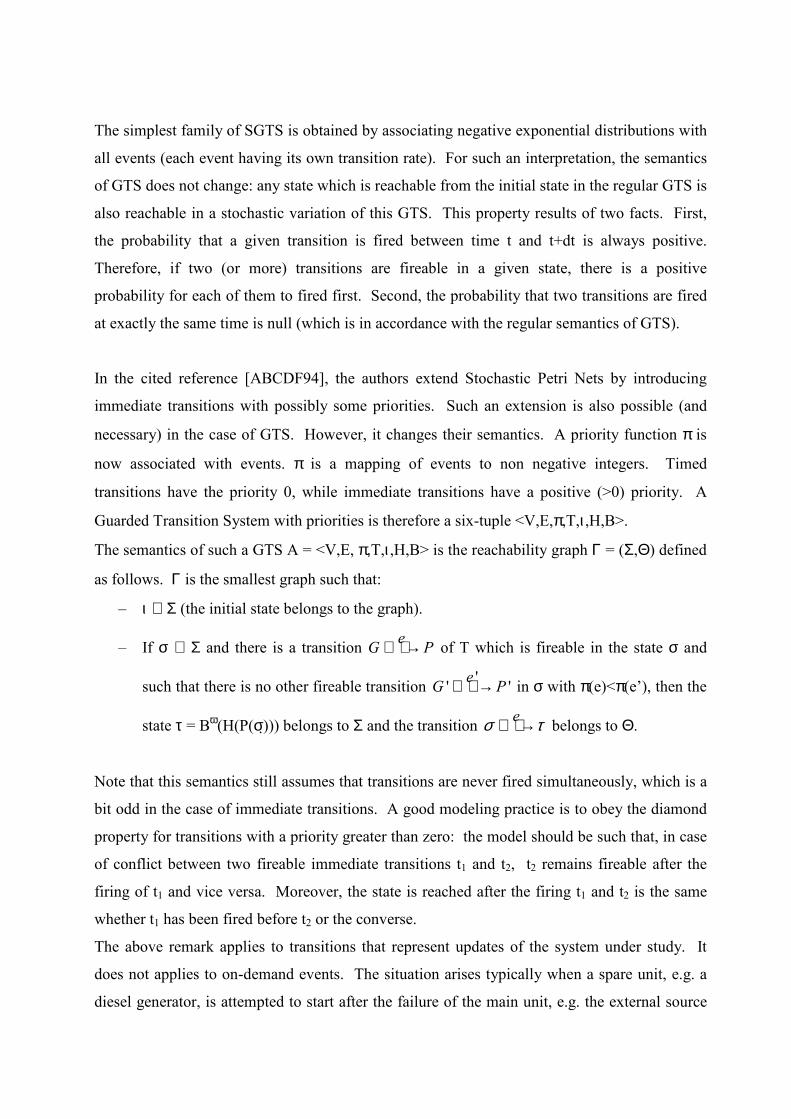
The simplest family of SGTS is obtained by associating negative exponential distributions with
all events (each event having its own transition rate). For such an interpretation, the semantics
of GTS does not change: any state which is reachable from the initial state in the regular GTS is
also reachable in a stochastic variation of this GTS. This property results of two facts. First,
the probability that a given transition is fired between time t and t+dt is always positive.
Therefore, if two (or more) transitions are fireable in a given state, there is a positive
probability for each of them to fired first. Second, the probability that two transitions are fired
at exactly the same time is null (which is in accordance with the regular semantics of GTS).
In the cited reference [ABCDF94], the authors extend Stochastic Petri Nets by introducing
immediate transitions with possibly some priorities. Such an extension is also possible (and
necessary) in the case of GTS. However, it changes their semantics. A priority function π is
now associated with events. π is a mapping of events to non negative integers. Timed
transitions have the priority 0, while immediate transitions have a positive (>0) priority. A
Guarded Transition System with priorities is therefore a six-tuple <V,E,π,T,ι,H,B>.
The semantics of such a GTS A = <V,E, π,T,ι,H,B> is the reachability graph Γ = (Σ,Θ) defined
as follows. Γ is the smallest graph such that:
– ι ∈ Σ (the initial state belongs to the graph).
– If σ ∈ Σ and there is a transition eG P→ of T which is fireable in the state σ and
such that there is no other fireable transition '
' 'e
G P→ in σ with π(e)<π(e’), then the
state τ = Bω(H(P(σ))) belongs to Σ and the transition eσ τ→ belongs to Θ.
Note that this semantics still assumes that transitions are never fired simultaneously, which is a
bit odd in the case of immediate transitions. A good modeling practice is to obey the diamond
property for transitions with a priority greater than zero: the model should be such that, in case
of conflict between two fireable immediate transitions t1 and t2, t2 remains fireable after the
firing of t1 and vice versa. Moreover, the state is reached after the firing t1 and t2 is the same
whether t1 has been fired before t2 or the converse.
The above remark applies to transitions that represent updates of the system under study. It
does not applies to on-demand events. The situation arises typically when a spare unit, e.g. a
diesel generator, is attempted to start after the failure of the main unit, e.g. the external source

of power. In such a situation, there is two conflicting immediate transitions (typically labeled
with events ‘start-on-demand’ and ‘fail-on-demand’). These two transitions are exclusive one
another. Moreover, a random choice has to be done among them. The existence of this kind of
immediate transitions does change the semantics in terms of reachability graph. However,
these transitions have clearly to be modeled in a separate way.
The following taxonomy can be established among transitions of SGTS.
– Immediate transitions can be split into two categories: plain immediate transitions,
which should obey the diamond property, and conditional (or on-demand) transitions.
Both of them can be given a priority. Conditional transitions come in groups. In a
group, all transitions should have the same guard and the same priority. When
performing a stochastic simulation, the probability to pick up a specific transition can be
defined by associating a weight to each transition of the group.
– Timed transitions can be split into two categories: Dirac transitions, which are fired
after a deterministic (positive) delay, and regular timed transitions whose probability
distribution is typically a negative exponential distribution or Weibull distribution.
Dirac transitions raise the same problem as immediate transitions: they can be fired at the same
instant, so a good modeling practice is that they should obey the diamond property. They raise
an additional problem: GTS with priorities are not sufficient to give their semantics, once
delays have been abstracted out. If two Dirac transitions with different delays are in conflict,
the one with the shortest delay will always be fired.
To finish, note that parameters of probability distributions may depend on the current state, i.e.
may be defined using variables.
6. Towards Semi-Formal Graphical Representations
As already said, graphics are very useful to present models. They are certainly a major reason
of the success of Fault Trees, Block Diagrams and Petri Nets. When modeling a complex
system however, we reach quickly the limits of drawings. First, the model does not fit on a
single sheet of paper or computer screen. To a large extent, this problem can be solved by
splitting the model into displayable parts and using references. Second and more important,
drawings cannot capture all aspects of the model. As an illustration, consider the small systems
we used so far. The Block Diagram pictured Figure 1 is very useful to understand the global
structure of the system, but it tells nothing about the behavior of nodes and edges. This
behavior could be described by a state graph or a Petri Net, but mixing the two kinds of
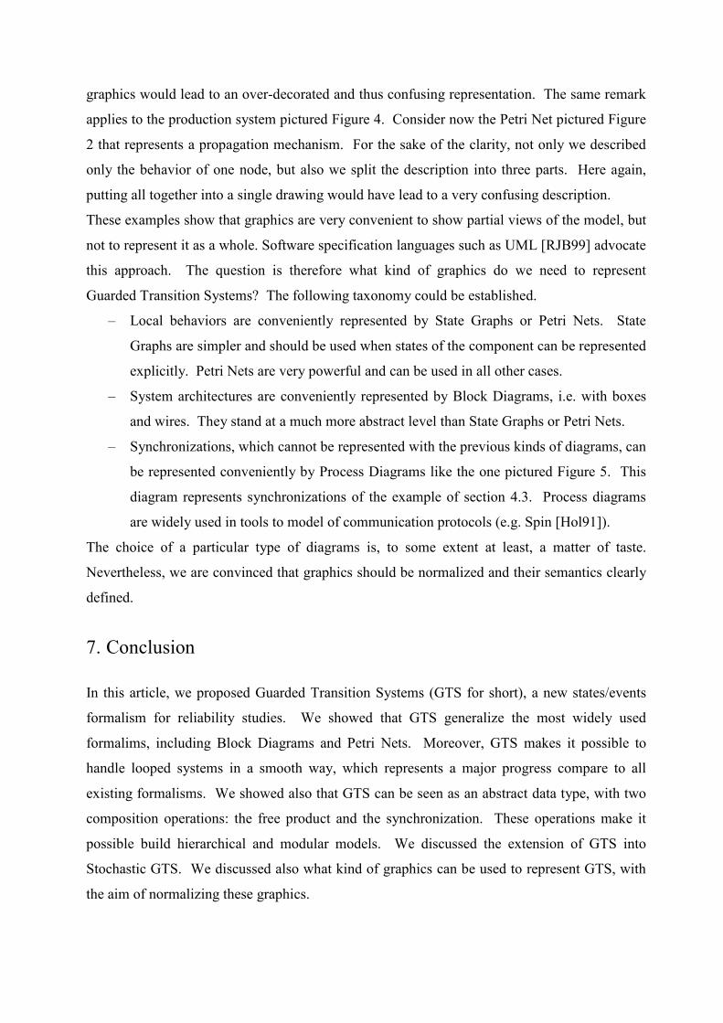
graphics would lead to an over-decorated and thus confusing representation. The same remark
applies to the production system pictured Figure 4. Consider now the Petri Net pictured Figure
2 that represents a propagation mechanism. For the sake of the clarity, not only we described
only the behavior of one node, but also we split the description into three parts. Here again,
putting all together into a single drawing would have lead to a very confusing description.
These examples show that graphics are very convenient to show partial views of the model, but
not to represent it as a whole. Software specification languages such as UML [RJB99] advocate
this approach. The question is therefore what kind of graphics do we need to represent
Guarded Transition Systems? The following taxonomy could be established.
– Local behaviors are conveniently represented by State Graphs or Petri Nets. State
Graphs are simpler and should be used when states of the component can be represented
explicitly. Petri Nets are very powerful and can be used in all other cases.
– System architectures are conveniently represented by Block Diagrams, i.e. with boxes
and wires. They stand at a much more abstract level than State Graphs or Petri Nets.
– Synchronizations, which cannot be represented with the previous kinds of diagrams, can
be represented conveniently by Process Diagrams like the one pictured Figure 5. This
diagram represents synchronizations of the example of section 4.3. Process diagrams
are widely used in tools to model of communication protocols (e.g. Spin [Hol91]).
The choice of a particular type of diagrams is, to some extent at least, a matter of taste.
Nevertheless, we are convinced that graphics should be normalized and their semantics clearly
defined.
7. Conclusion
In this article, we proposed Guarded Transition Systems (GTS for short), a new states/events
formalism for reliability studies. We showed that GTS generalize the most widely used
formalims, including Block Diagrams and Petri Nets. Moreover, GTS makes it possible to
handle looped systems in a smooth way, which represents a major progress compare to all
existing formalisms. We showed also that GTS can be seen as an abstract data type, with two
composition operations: the free product and the synchronization. These operations make it
possible build hierarchical and modular models. We discussed the extension of GTS into
Stochastic GTS. We discussed also what kind of graphics can be used to represent GTS, with
the aim of normalizing these graphics.

GTS are thus a powerful modeling formalism. For most of the assessment algorithms,
including sequence generations and Monte-Carlo simulation, there is no increase in complexity
of the treatments. Two problems remain open however. First, does the algorithm to compile
Mode Automata into Fault Tree (proposed by the author in reference [Rau02]) extends to GTS?
This is an important question with respect to the assessment of large industrial systems. The
second problem is raised by the introduction of Dirac transitions. Assume that transitions are
either immediate, or timed with a negative exponential distribution, or Dirac transitions. Under
which condition is it possible to interpret the GTS as a multiphase Markov process and what is
the compilation algorithm? This question is of primary importance for the modeling of systems
with periodically tested components. We shall discuss it in a forthcoming article.
Engine 1 Engine 2 RepairCrew
startRepair startJob
endRepair endJob
startRepair startJob
endRepair endJob
Figure 5. A Synchronization Diagram
8. References
[ABCDF94] M. AjmoneMarsan, G. Balbo, G. Conte, S. Donatelli, and G. Franceschinis.
Modelling with Generalized Stochastic Petri Nets. Wiley Series in Parallel Computing.
John Wiley and Sons, 1994.
[AM93] J.D. Andrews and T.R. Moss. Reliability and Risk Assessment. John Wiley & Sons,
1993. ISBN 0-582-09615-4.

[Arn94] A. Arnold. Finite Transition Systems. C.A.R Hoare. Prentice Hall, 1994. ISBN 0-13-
092990-5.
[Bal86] M.O. Ball. Computational complexity of network reliability analysis: an overview.
IEEE Transactions on Reliability, R-35:230–239, 1986.
[BRDS04] M. Boiteau, Y. Dutuit, A. Rauzy and J.-P. Signoret, The AltaRica Data-Flow
Language in Use: Assessment of Production Availability of a MultiStates System,
Reliability Engineering and System Safety, Vol. 91, pp 747-755, Elsevier.
[Col87] C.J. Colbourn. The combinatorics of network reliability. Oxford University Press, New
York, 1987.
[Esp98] J. Esperza, Decidability and Complexity of Petri Nets Problems – An introduction, Lectures on Petri Nets I: Basic Models, in W. Reisig and G. Rozenberg, LNCS 1491, pp
374-428, Springer, ISBN 3-540-65306-6, 1998
[Hol91] G.J. Holzmann. Design and validation of computer protocols. software series. Prentice
hall, 1991. ISBN 0-13-539925-4.
[KR02] Y. Kawauchi and M. Rausand, A new approach to production regularity assessment in
the oil and chemical industries. Reliability Engineering and System Safety, n°75 pp 379–
388, 2002.
[vLeu90] J. Van Leuwen, editor, Handbook of Theoretical Computer Science, volume B,.
Elsevier, 1990.
[MCFB94] J.-C. Madre, O. Coudert, H. Fraïssé, and M. Bouissou. Application of a New
Logically Complete ATMS to Digraph and Network-Connectivity Analysis. In
Proceedings of the Annual Reliability and Maintainability Symposium, ARMS'94, pages
118–123, 1994. Annaheim, California.
[Pap94] C.H. Papadimitriou. Computational Complexity. Addison Wesley, 1994. ISBN 0-201-
53082-1.
[Rau02] A. Rauzy. Mode automata and their compilation into fault trees. Reliability
Engineering and System Safety, Elsevier, Volume 78, Issue 1, pp 1-12, 2002.
[RJB99] J. Rumbaugh and I. Jacobson and G. Booch, The Unified Modeling Language.
Reference Manual, Addison Wesley, ISBN 0-201-30998-X, 1999
[Shi91] D.R. Shier. Network Reliability and Algebraic Structures. Oxford Science Publications,
1991.
[SBT96] T.R. Shiple, G. Berry, and H. Touati. Constructive Analysis of Cyclic Circuits. In
Proc. International Design and Testing Conf (ITDC), Paris, March 1996.
[SSBS96] T. R. Shiple, V. Singhal, R. K. Brayton, and A. L. Sangiovanni-Vincentelli. Analysis
of Combinational Cycles in Sequential Circuits. In Proc. Intl. Symposium on Circuits and
Systems, Atlanta, GA, May 1996.