Guaranteeing Method for the Stability of Cluster Structure...
10
Guaranteeing Method for the Stability of Cluster Structure Formed by Autonomous Decentralized Clustering Mechanism Ryo Hamamoto 1 , Chisa Takano 1 , Kenji Ishida 1 , and Masaki Aida 2 1 Graduate School of Information Sciences, Hiroshima City University, Hiroshima-shi, Hiroshima, 731-3194 Japan 2 Graduate School of System Design, Tokyo Metropolitan University, Hino-shi, 191-0065 Japan Email: [email protected]; {takano, ishida}@hiroshima-cu.ac.jp; [email protected] Abstract —Mobile ad hoc networks (MANETs) can be configured by mobile terminals without any network infrastructure such as Access Points (APs), and they are expected to be a useful tool during serious disasters such as a large earthquake. Many studies have concentrated on clustering methods that aim at power saving and loadbalancing in MANETs. For the clustering mechanism of a MANET, we have proposed an autonomous decentralized structure formation method based on the local interaction of terminals and have used this method to create an autonomous decentralized clustering of MANETs. However, the problem of our proposed clustering method is that the number of clusters decreases with temporal evolution. The power saving and the load balancing by the hierarchical management of the network cannot be performed by this problem. This paper proposes a method which maintains the number of clusters (guarantees stability). Index Terms—Autonomous decentralized control, localaction theory, ad hoc network, clustering I. INTRODUCTION When almost all network infrastructure is destroyed by a serious disaster, it is necessary to create an environment in which the remaining devices can operate effectively and distribute information quickly in order to support smooth disaster restoration activities. Mobile ad hoc networks (MANETs) [1] have received significant attention in recent years for such an emergency situation. MANETs directly connect network terminals to each other without network infrastructure such as wireless LAN access points. At the time of a disaster, reducing the power consumption of terminals is very important. Many studies have concentrated on clustering methods that aim at power saving and load balancing in MANETs [2]. Here, clustering methods divide the network to multiple subnetworks (clusters) and realize hierarchical management for the inter-cluster and the intra-cluster. Power saving and load balancing are crucial because they make it possible to reduce the power consumption of each Manuscript received January 11, 2015; revised August 19, 2015. This research was partly supported by JSPS KAKENHI Grant Numbers 26280032, 15K00431, and Project Research Grants from the Graduate School of Information Sciences, Hiroshima City University. Corresponding author email: [email protected] doi:10.12720/jcm.10.8.562-571. node and extend the life of the network after a disaster. Some clustering methods realize both by using metrics such as each node’s battery reserves [3] and performance [4]. Generally, global network state information is required to optimize the cluster structure. However, in MANETs, information exchange is structurally limited, and each node needs to execute traffic control, path control, and network resource management using only local information. Many studies have targeted the clustering algorithm [5]–[7]. However, since their algorithms require non- local information, they are not “strictly” autonomous decentralized algorithms. The common basic attribute demanded from these algorithms in addition to locality is adaptability to the network environment. Each node has its specific situation that influences the formation of clusters. So, it is preferable for the clustering mechanism to take the situations of individual nodes into consideration. [8], [9] can configure clusters through only local information by the well-known bio-inspired approach that uses Turing patterns formed by reaction- diffusion equations. However, this method cannot yield cluster structures that reflect the characteristics of the given environmental conditions (e.g. the distribution of the residual battery power of terminals, the position of power supplies, or the node degree of mobile terminals) [10]. Moreover, because this method uses seven parameters, it is difficult to identify the appropriate values for these multiple parameters. [10]–[12] have already proposed a framework of autonomous decentralized control based on local interaction as a novel control mechanism. This framework is based on the relationship between the local interaction and the solution provided by a partial differential equation. As a specific example, [10] have proposed the autonomous decentralized formation of structures with finite spatial size and showed that proposal’s applicability to autonomous decentralized clustering in ad hoc networks. The clustering method of [10] allows the nodes to act flexibly in a manner based only on the information each individual node is aware of, i.e. its individual situation, and it can yield cluster structures that reflect the characteristics of the given environmental conditions. In [13], the method of [10] can 562 Journal of Communications Vol. 10, No. 8, August 2015 ©2015 Journal of Communications
Transcript of Guaranteeing Method for the Stability of Cluster Structure...

Guaranteeing Method for the Stability of Cluster Structure
Formed by Autonomous Decentralized Clustering
Mechanism
Ryo Hamamoto1, Chisa Takano
1, Kenji Ishida
1, and Masaki Aida
2
1 Graduate School of Information Sciences, Hiroshima City University, Hiroshima-shi, Hiroshima, 731-3194 Japan
2 Graduate School of System Design, Tokyo Metropolitan University, Hino-shi, 191-0065 Japan
Email: [email protected]; {takano, ishida}@hiroshima-cu.ac.jp ; [email protected]
Abstract—Mobile ad hoc networks (MANETs) can be
configured by mobile terminals without any network
infrastructure such as Access Points (APs), and they are
expected to be a useful tool during serious disasters such as a
large earthquake. Many studies have concentrated on clustering
methods that aim at power saving and loadbalancing in
MANETs. For the clustering mechanism of a MANET, we have
proposed an autonomous decentralized structure formation
method based on the local interaction of terminals and have
used this method to create an autonomous decentralized
clustering of MANETs. However, the problem of our proposed
clustering method is that the number of clusters decreases with
temporal evolution. The power saving and the load balancing by
the hierarchical management of the network cannot be
performed by this problem. This paper proposes a method
which maintains the number of clusters (guarantees stability).
Index Terms—Autonomous decentralized control, localaction
theory, ad hoc network, clustering
I. INTRODUCTION
When almost all network infrastructure is destroyed by
a serious disaster, it is necessary to create an environment
in which the remaining devices can operate effectively
and distribute information quickly in order to support
smooth disaster restoration activities. Mobile ad hoc
networks (MANETs) [1] have received significant
attention in recent years for such an emergency situation.
MANETs directly connect network terminals to each
other without network infrastructure such as wireless
LAN access points. At the time of a disaster, reducing the
power consumption of terminals is very important. Many
studies have concentrated on clustering methods that aim
at power saving and load balancing in MANETs [2]. Here,
clustering methods divide the network to multiple
subnetworks (clusters) and realize hierarchical
management for the inter-cluster and the intra-cluster.
Power saving and load balancing are crucial because they
make it possible to reduce the power consumption of each
Manuscript received January 11, 2015; revised August 19, 2015.
This research was partly supported by JSPS KAKENHI Grant Numbers 26280032, 15K00431, and Project Research Grants from the
Graduate School of Information Sciences, Hiroshima City University. Corresponding author email: [email protected]
doi:10.12720/jcm.10.8.562-571.
node and extend the life of the network after a disaster.
Some clustering methods realize both by using metrics
such as each node’s battery reserves [3] and performance
[4]. Generally, global network state information is
required to optimize the cluster structure. However, in
MANETs, information exchange is structurally limited,
and each node needs to execute traffic control, path
control, and network resource management using only
local information.
Many studies have targeted the clustering algorithm
[5]–[7]. However, since their algorithms require non-
local information, they are not “strictly” autonomous
decentralized algorithms. The common basic attribute
demanded from these algorithms in addition to locality is
adaptability to the network environment. Each node has
its specific situation that influences the formation of
clusters. So, it is preferable for the clustering mechanism
to take the situations of individual nodes into
consideration. [8], [9] can configure clusters through only
local information by the well-known bio-inspired
approach that uses Turing patterns formed by reaction-
diffusion equations. However, this method cannot yield
cluster structures that reflect the characteristics of the
given environmental conditions (e.g. the distribution of
the residual battery power of terminals, the position of
power supplies, or the node degree of mobile terminals)
[10]. Moreover, because this method uses seven
parameters, it is difficult to identify the appropriate
values for these multiple parameters.
[10]–[12] have already proposed a framework of
autonomous decentralized control based on local
interaction as a novel control mechanism. This
framework is based on the relationship between the local
interaction and the solution provided by a partial
differential equation. As a specific example, [10] have
proposed the autonomous decentralized formation of
structures with finite spatial size and showed that
proposal’s applicability to autonomous decentralized
clustering in ad hoc networks. The clustering method of
[10] allows the nodes to act flexibly in a manner based
only on the information each individual node is aware of,
i.e. its individual situation, and it can yield cluster
structures that reflect the characteristics of the given
environmental conditions. In [13], the method of [10] can
562
Journal of Communications Vol. 10, No. 8, August 2015
©2015 Journal of Communications

configure clusters faster than an existing method [8] by a
factor of 10 or more. This means that communication can
be recovered more quickly by the method of [10].
However, the problem of [10] is that the number of
clusters decreases with temporal evolution. The power
saving and the load balancing by the hierarchical
management of the network cannot be performed by this
problem. This paper proposes a method which maintains
the number of clusters (guarantees stability). So, our aim
is to maintain the hierarchical network configuration
created by clusters. Our study focuses on the hierarchical
network configuration that is the preliminary study
needed to realize the real communication considering
data transfer by network protocols.
This paper consists of the following sections. In Sec. II,
we present the framework of our proposed autonomous
decentralized structure formation method, and we discuss
the issues for this method. In Sec. III, we propose a
method of guaranteeing the stability by preserving the
history of the distribution. We evaluate the characteristics
of the proposed method in Sec. IV, and Sec. V presents
the concluding remarks.
II. CLUSTERING M AUTONOMOUS
DECENTRALIZED STRUCTURE FORMATION
This section overviews the autonomous decentralized
structure formation proposal [10] that uses the diffusion
and the drift (back diffusion). Moreover, we describe the
problem of our structure formation method that is applied
to clustering in MANET.
A. Overview of the Autonomous Decentralized
Structureformation Method
First, we introduce the autonomous decentralized
structure formation method for a one-dimensional
network model to understand the behavior of our
proposal intuitively. Let the density function (density
distribution) of a certain quantity at time t and position x
be q(x, t). The initial value of q(x, 0) can be considered as
the metric, for example, the residual battery life of each
node in an MANET. Local behavior corresponds to
changing the value of q(x, t) at each point, x, by
controlling the information exchange between adjacent
nodes. In the autonomous decentralized structure
formation, the flow J(x, t) (the operation rule that changes
the value of q(x, t)) is expressed as
(1)
where the first and the second terms denote the drift and
diffusion terms, respectively. The temporal evolution of
the distribution q(x, t) that corresponds to this change is
given by
(2)
c (> 0) denotes the rate of the temporal evolution of q(x, t)
and denotes the variance of the normal distribution
that is converged on. J(x, t) represents the amount of
spatial movement of q(x, t); note that the total amount of
q(x, t) does not change over time. Equation (2) is a
second-order differential equation. Therefore, this
operation rule can be determined by interaction with the
adjacent nodes.
The introduction of f(x, t) eliminates the need to set a
coordinate system in the network. As a more intuitive
explanation, we consider the potential function
instead of the function f(x, t):
(3)
Choosing appropriately yields autonomous
decentralized control that does not depend on a
coordinate system. We consider how to determine the
drift term from q(x, t) at each point x. Because
should result in maintaining the distribution within a
certain finite spatial size, contrary to the effect of
diffusion, is, after a discrete time , given by
(4)
where , and is periodically renewed at
intervals of . This equation is obtained by the sign
inversion of the space derivative term in the diffusion
equation. Note that in Eq. (4), we use a periodical time
with interval instead of dt. This is because the effect
of the second term vanishes in the limit that dt
approaches 0 [10].
Fig. 1. Determining according to back diffusion.
Fig. 2. Diffusion and back diffusion.
The method of generating the potential
by using q(x, t) is shown in Fig. 1. The meaning of this
figure is expressed as follows:
We let the time progression of the diffusion
phenomenon with diffusion coefficient be reversed
(back diffusion).
563
Journal of Communications Vol. 10, No. 8, August 2015
©2015 Journal of Communications
ETHOD ON ASEDB
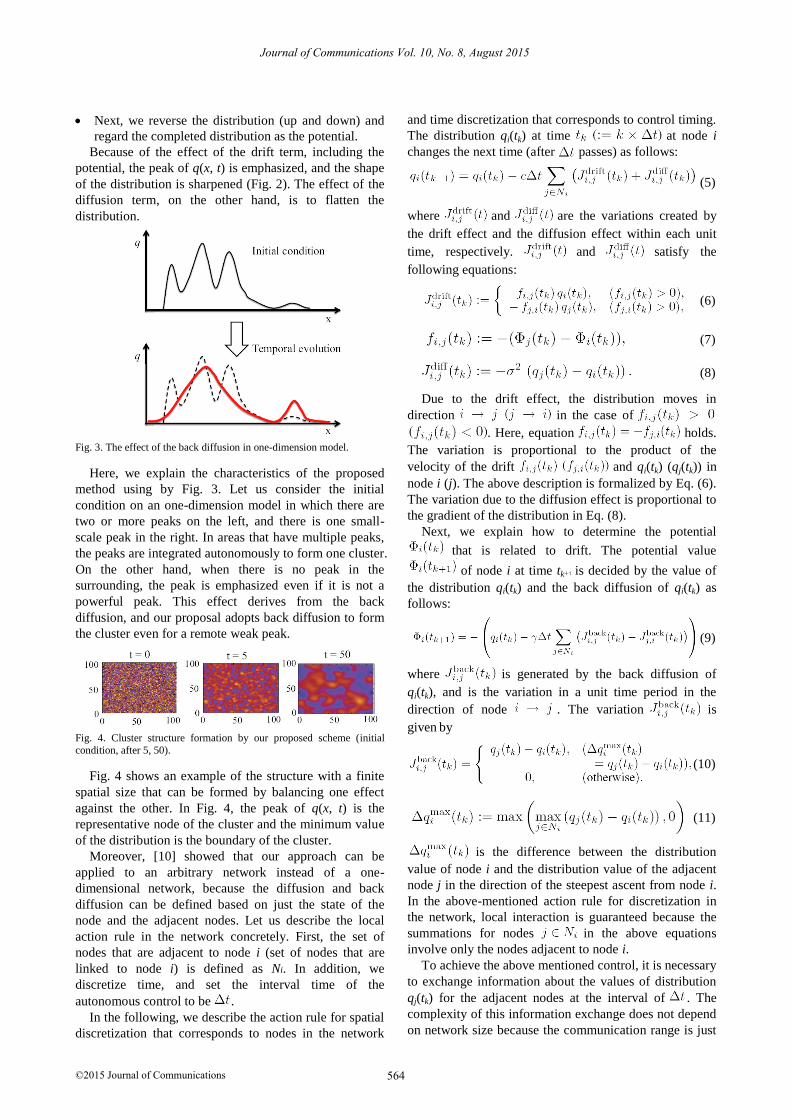
Next, we reverse the distribution (up and down) and
regard the completed distribution as the potential.
Because of the effect of the drift term, including the
potential, the peak of q(x, t) is emphasized, and the shape
of the distribution is sharpened (Fig. 2). The effect of the
diffusion term, on the other hand, is to flatten the
distribution.
Fig. 3. The effect of the back diffusion in one-dimension model.
Here, we explain the characteristics of the proposed
method using by Fig. 3. Let us consider the initial
condition on an one-dimension model in which there are
two or more peaks on the left, and there is one small-
scale peak in the right. In areas that have multiple peaks,
the peaks are integrated autonomously to form one cluster.
On the other hand, when there is no peak in the
surrounding, the peak is emphasized even if it is not a
powerful peak. This effect derives from the back
diffusion, and our proposal adopts back diffusion to form
the cluster even for a remote weak peak.
Fig. 4. Cluster structure formation by our proposed scheme (initial
condition, after 5, 50).
Fig. 4 shows an example of the structure with a finite
spatial size that can be formed by balancing one effect
against the other. In Fig. 4, the peak of q(x, t) is the
representative node of the cluster and the minimum value
of the distribution is the boundary of the cluster.
Moreover, [10] showed that our approach can be
applied to an arbitrary network instead of a one-
dimensional network, because the diffusion and back
diffusion can be defined based on just the state of the
node and the adjacent nodes. Let us describe the local
action rule in the network concretely. First, the set of
nodes that are adjacent to node i (set of nodes that are
linked to node i) is defined as Ni. In addition, we
discretize time, and set the interval time of the
autonomous control to be .
In the following, we describe the action rule for spatial
discretization that corresponds to nodes in the network
and time discretization that corresponds to control timing.
The distribution qi(tk) at time at node i
changes the next time (after passes) as follows:
(5)
where and are the variations created by
the drift effect and the diffusion effect within each unit
time, respectively. and satisfy the
following equations:
(6)
(7)
(8)
Due to the drift effect, the distribution moves in
direction in the case of
. Here, equation holds.
The variation is proportional to the product of the
velocity of the drift and qi(tk) (qj(tk)) in
node i (j). The above description is formalized by Eq. (6).
The variation due to the diffusion effect is proportional to
the gradient of the distribution in Eq. (8).
Next, we explain how to determine the potential
that is related to drift. The potential value
of node i at time tk+1 is decided by the value of
the distribution qi(tk) and the back diffusion of qi(tk) as
follows:
(9)
where is generated by the back diffusion of
qi(tk), and is the variation in a unit time period in the
direction of node . The variation is
given by
(10)
(11)
is the difference between the distribution
value of node i and the distribution value of the adjacent
node j in the direction of the steepest ascent from node i.
In the above-mentioned action rule for discretization in
the network, local interaction is guaranteed because the
summations for nodes in the above equations
involve only the nodes adjacent to node i.
To achieve the above mentioned control, it is necessary
to exchange information about the values of distribution
qj(tk) for the adjacent nodes at the interval of . The
complexity of this information exchange does not depend
on network size because the communication range is just
564
Journal of Communications Vol. 10, No. 8, August 2015
©2015 Journal of Communications

1 hop. Therefore, it is scalable against the number of
nodes.
Note that, needs to satisfy Eq. (12)
(12)
where dmax means the maximum degree of nodes in the
network. If do not meet Eq. (12), q(.) of some nodes
become negative value by the diffusion effect [14].
B. Problems with Applying the Proposal to Clustering
In this section, we discuss the issues raised by applying
this technology to MANETs. The autonomous
decentralized structure formation proposal described in
Sec. II-A forms some clusters by balancing the diffusion
term (diffusion effect of the distribution) against the drift
term (emphasizing effect of the peak of the distribution).
If the diffusion effect is greater than the drift effect, the
distribution of the formed structure is smoothed over time
and the range of the distribution decays (Fig. 5). Here, the
range R(t) denotes the difference in the maximum value
and the minimum value of the distribution for each time
as below:
(13)
Fig. 5. Issues in parameter setting.
On the other hand, if the drift effect is stronger than the
diffusion effect, the peak of the structure is emphasized,
and the unevenness of initial distribution becomes
excessive. Therefore, it is necessary to balance of the
strengths of the diffusion and drift terms, but designing
the optimum parameters is very difficult. Let us consider
the situation where the diffusion effect is stronger than
the drift effect. In that case, the range of the distribution
decays over time (Fig. 6). Note that we evaluate the
characteristics of the decay of the range in Sec. IV-A.
Fig. 6. Decay of the range of the distribution.
The decay characteristics cause two problems: First,
the representative nodes and the boundaries of clusters
cannot be determined when the range of the distribution
becomes zero (complete harmonization) by the diffusion
effect. In the mathematical expression, the complete
harmonization practically requires infinite time; however,
the range of the distribution becomes zero in finite time
owing to the limits of the calculation accuracy, which
means that the proposed method cannot configure the
clusters. That is, the power saving and the load balancing
by the hierarchical management of the network cannot be
performed by this problem. Second, we should consider a
situation where the distribution of one network is
compared to the distribution of another network. This
problem may occur in an MANET when new terminals
connect or other terminals move into the area under
consideration. For example, “network A” has a small
range of the distribution by the diffusion effect, whereas
“network B” has a large range of the distribution. Note
that this situation is that the initial range of the
distribution of “network A” is the same as that of
“network B,” but the range of the distribution of
“network A” decays because of a lapse of time from the
cluster formation and is smaller than that of “network B.”
When these networks merge, “network A” will not be
able to preserve its form, because their networks have the
different measures for the ranges of the distributions (Fig.
7). In other words, a cluster which has large range of the
distribution has a huge effect on the cluster compared to a
cluster which has small range of the distribution.
Fig. 7. Problems with dynamic network topologies.
III. METHOD GUARANTEEING STABILITY OF THE CLUSTER
STRUCTURE FOR A VECTOR PROCESS
In this section, we discuss the requirement that the
range of the distribution should satisfy in order to restrain
the decay of it, and then propose a method which meets
the requirement.
As mentioned in Sec. II-B, it is necessary to restrain
the decay of the range caused by the time progression in
order to maintain the cluster structure. This is the
requirement for the range of the distribution. To show the
requirement for the range of the distribution, we
introduce the asymptotic stability for the range of the
distribution as follows.
(14)
where R(t) is defined in Eq. (13) and is a positive
constant. This equation means that the range of the
distribution converges on a positive constant value over
infinite time. Unless it is satisfied, on the other hand, R(t)
approaches zero with time.
Next, we explain our method which restrains the decay
of the range and guarantees the asymptotic stability of the
range. To guarantee the stable range of the distribution,
each node has its own vector with N components to keep
565
Journal of Communications Vol. 10, No. 8, August 2015
©2015 Journal of Communications

the history information of the distribution. Each node has
its own value, p(tk), that denotes the distribution (for
example, battery residual power) at time .
Q(tk) shows the distribution used for configuring the
cluster structure at tk; it is given as follows:
(15)
(16)
The vector’s 0th component is set to p(tk). In each step,
the diffusion and drift (back diffusion) operations are
performed for every component of Q(tk). In other words,
each component of the vector is calculated by the
diffusion and the back diffusion. When the operations are
completed for every component of Q(tk), the nth
component of the vector is shifted to
the n + 1th component in the following step (Fig. 8). Note
that N + 1th component is discarded. If p(tk) does not
change over time, Q(tk) will not change either. A cluster
is constructed by using qn(tk) (a specified n within
) which each node has, and larger
clusters can be configured by specifying the larger n.
Fig. 8. Temporal evolution of Q(tk) for each node.
In general clustering, it is demanded that the number of
cluster heads (the representative nodes) in the network is
small (in other words, the average cluster size is large)
because nodes chosen as cluster heads have a heavy load
due to the management of the control information for
both the inter- and the intra-cluster. If the cluster size is
large (the number of clusters is small), on the other hand,
significant traffic occurring in bursts within the cluster
causes the overload of functions for the cluster head
because each cluster head attends to many member nodes
in the cluster. Here, the main purpose of this paper is not
to argue about the optimal cluster size. The purpose of
this paper is to maintain the hierarchical network
structure created by clusters. Note that our proposed
method can adjust the mean number of clusters to some
extent according to the network situation by only using
local information exchange. The vector process of our
proposed method can be simply expressed as follows:
Each node keeps N distribution values for each time by
using the vector structure qn(tk). The values have a hardly
diffused distribution when n is small and an almost
completely diffused distribution when n is large.
Here, Rn(tk) is the range of
thedistribution for the nth component at time tk as follows:
(17)
In our proposed method, if the distribution p(tk) (e.g.
the battery capacity) does not change with time, the
vector structure Q(tk) that each node keeps does not
change as well. That is to say, the asymptotic stability of
the range in Eq. (14) is expressed as follows:
(18)
where Rn(tk) can be calculated by Eq.(17), and tn is the
period of time used to form the n components of the
vector structure from nothing. Eq. (18) shows the
requirement to stabilize the range of the distribution not
“asymptotically” but “completely”, if nodes are
immovable and the initial distribution for each node does
not change. When the distribution p(tk) becomes smaller
with time, the decay of the range of the distribution
cannot be stopped, but our proposed method can restrain
the range decay phenomenon caused by diffusion effects.
The issue for our method is that a certain time tn is
required when creating a vector structure from nothing.
The range of the distribution decays by the diffusion
effect until the vector structure is formed. We will
address this issue in future work. In addition, our
proposed method can be applied to other clustering
methods [15].
IV. EVALUATION
In this section, we investigate the decay characteristics
of the range of the distribution shown in Sec.II-B, and we
evaluate the stability of the proposed method using a two-
dimensional lattice model and an MANET model.
A. Decay Characteristics of the Range
First, we examine the decay characteristics of the range
drift effect and diffusion effect. As preliminary research,
we assume a two-dimensional lattice model with 100 ×
100 nodes to make the space structure easy to display.
The network model has a torus topology to exclude the
influence of the boundary (Fig. 9). Each node has a
degree of four (dmax = 4) because each node has four
neighbors, and sends a control packet to their neighbors
at every step ( = 1 step), which is the normalized time.
In this evaluation, the node sends control parameters for
adjacent nodes at the same time. Moreover, each node
does not move in this evaluation. Our assumed initial
state of the distribution is the state where clusters have
been already formed to some extent (Fig. 10). Because
the purpose of the study is to investigate the range
characteristics of the distribution due to the diffusion
effect and the drift effect, intense unevenness of the
initial state of the distribution quantity is not needed. The
horizontal and vertical axes in Fig. 10 represent the
coordinates, and the color of each node indicates the
distribution height.
566
Journal of Communications Vol. 10, No. 8, August 2015
©2015 Journal of Communications

Fig. 9. Torus topology.
Fig. 10. Initial conditions (1).
Fig. 11. Temporal variation of the distribution range due to diffusion.
Fig. 12. Damping characteristics in the distribution range due to
diffusion.
TABLE I: EXPERIMENTAL PARAMETERS (DIFFUSION ONLY)
Fig. 11 shows the temporal variation of the range of
the distribution due to the diffusion effect (without the
drift effect). This figure is a semilog plot, and the unit of
time is the number of steps. Each node computes its own
distribution at every step. The parameters used are listed
in Table I. It is seen that exponential decay occurs
regardless of the value of . The relationship of and
the decay rate is shown in Fig. 12; is proportional to
the decay rate of the diffusion effect.
Fig. 13 is a representation of the temporal variation of
the range of the distribution due to the diffusion and drift
effects. The parameters used in the simulation are =
0.01 and = 0.1; c is varied. This figure is a semilog plot,
and the unit of time is the number of steps. We can see
from this figure that exponential decay occurs regardless
of the value of c. Fig. 14 shows the relation of the decay
rate and c. From these results, c is proportional to the
decay rate for the diffusion and drift effects.
Fig. 13. Temporal variation of the distribution range due to diffusion
and drift.
Fig. 14. Relation of the decay rate and c in the distribution range due to diffusion and drift.
As mentioned above, the range of the distribution
exponentially decays with time and will become zero
within finite time, that is to say that it does not satisfy the
asymptotic stability shown in Eq. (14).
Next, we evaluate the characteristics of the decay for
the proposed method using the vector process in Sec. III
and the existing method. We assume two situations:
The initial distribution, p(tk), (ex. residual battery
power) does not change over time, and all nodes are
immovable (Sec. IV-B)
The initial distribution, p(tk), decreases gradually by
power consumption, and all nodes can move (Sec. IV-
C)
B. Evaluation of Stability (in Two-Dimensional Lattice
Model)
We assume a two-dimensional lattice model with 100
× 100 nodes in a torus topology; nodes do not move
567
Journal of Communications Vol. 10, No. 8, August 2015
©2015 Journal of Communications

(fixed nodes). The ith node’s initial distribution (the
initial battery capacity), pi(0), is set to a random number
uniformly distributed in [10, 20] (Fig. 15). In this
experiment, pi(tk) does not change over time. Furthermore,
nodes in the network do not move in this simulation. The
parameters used are summarized in Table II, and the
number of components of the vector for the proposed
clustering model is 21 . These
parameters satisfy the conditions of Eq.(12). For these
parameters, the range of the distribution is due to the
diffusion effect being greater than the drift effect [10].
Each node sends control packets every 1 s ( = 1 s) and
deals with the diffusion and drift processing on the basis
of the information in the received packets. In our
evaluation, the node sends control parameters for its
adjacent nodes at the same time. Moreover, the
simulation time is 1:0 hour.
TABLE II: EXPERIMENTAL PARAMETERS (THE TWO-DIMENSIONAL
NETWORK Q DOES NOT CHANGE OVER TIME)
Fig. 15. Initial conditions (2).
Fig. 16 shows the cluster structures for the 5th and
20th components of the vector at time tk (tk = 0.1, 0.5, 1.0
hour). We can see from this figure that the cluster of the
5th component has a finer structure than that of the 20th
component. This is because the latter is strongly
influenced by the diffusion effect. In other words, if we
set the vector component’s number to a large value, we
can configure larger clusters.
Fig. 16. Cluster structures for the 5th and 20th components of Q(tk).
Fig. 17 shows the temporal variation in the distribution
range for the 5th and 20th components of Q(tk). This
figure includes results for the existing method [10] for
comparison with our proposal. We can see from this
figure that the range of the distribution for the existing
method always decays, which means that the existing
method cannot guarantee the stability for the range of the
distribution shown in Eq. (14).
Fig. 17. Temporal variation in the distribution range for the 5th and 20th
components of Q(tk).
For our proposed method, on the other hand, the range
of the distribution is “completely” stable (guarantees the
stability in Eq. (18)) after time tn, which is the period of
time needed to form the n components of the vector
structure from nothing, because the initial value of the
distribution of each node does not change over time. In
the case with the 5th and 20th components, tn = 5 × 1 s= 5
s and tn = 20 × 1 s = 20 s, respectively.
TABLE III: THE CONVERGED VALUE OF THE RANGE .
Moreover, Table III shows the converged value of the
range of the distribution in each component of the vector.
This result shows that the converged value of the 5th
component is greater than that of the 20th component,
because the latter is strongly influenced by the diffusion
effect.
C. Evaluation of Stability (in MANET)
In this section, we evaluate the decay characteristics of
the proposed method in a network model supposing an
MANET. The network model is the unit disk graph
(UDG) with dimensions of 1, 500 m × 1, 500 m and a
torus topology (Fig. 18). UDG is a type of intersection
graph based on circles of the same size. UDG is suitable
as a model of an ad hoc network because it can describe
various radio transmission ranges between nodes, but it
cannot reflect more realistic wireless network
characteristics such as packet collisions. We will address
this issue in future work.
Fig. 18. Unit disc graph network.
568
Journal of Communications Vol. 10, No. 8, August 2015
©2015 Journal of Communications

The simulation conditions are as follows. 100 nodes
are randomly placed in the area. The initial distribution
pi(0) for node i is a uniform random number in the range
of [10, 20] (Fig. 19); the radio transmission range for
each node is 250 m. Regarding mobility, all nodes move
every 100 s, 10 s, or 1 s in consideration of the
convergence time of cluster formation. The range to
which each node moves at the above intervals yields an
average movement distance of 1.3 m (uniform random
number [0, 2.6]); the direction is based on the random
direction model. The parameters of the proposed model
are listed in Table IV. Note that, these parameters meet
the conditions of Eq.(12). We assume that the initial
distribution of each node, is identical to the random initial
battery capacity, and the battery capacity of each node
decreases by transmitting and processing control packets
to and from neighbor nodes. Each node sends control
packets every 1 s ( = 1 s) and deals with the diffusion
and drift processing on the basis of the information in the
received packets. Note that the node sends control
packets for adjacent nodes simultaneously. Each node
consumes the battery reserves at 1 J/bit for the
transmission and reception of packets, and that of each
representative node is 0.1 J/s for processing, which is
self-performed [16]. In addition, the distribution pi(tk) of
node i is the residual battery capacity at tk. We assume
that nodes whose residual battery capacities become zero
become unavailable and secede from the network. We
pay attention to the decay characteristics of the range of
the cluster configured by the 5th and 20th components.
Note that, in the case with the 5th and 20th components,
tn = 5×1 s = 5 s and tn = 20×1 s = 20 s, respectively.
Fig. 19. Initial conditions (3).
TABLE IV: EXPERIMENTAL PARAMETERS (MANET Q CHANGES OVER
TIME).
Fig. 20, Fig. 21, and Fig. 22 show temporal variation in
the distribution range for the 5th and 20th components for
each mobility frequency. In these figures, the horizontal
axis and vertical axis represent time and the range of the
distribution, respectively. These results show that the
range of the distribution for the existing method
decreases sharply regardless of the node mobility
frequency. The range for the existing method approaches
zero very fast, and the existing method can not guarantee
the stability in Eq. (14). On the other hand, the
characteristics of the range for our proposed method
maintain nearly a fixed value after time tn (tn = 5 or 20 s)
for all patterns of the node mobility frequency. The
proposed method does not satisfy Eq. (18), but it can
maintain the range of the distribution at a positive value
for a long time. Table V summarizes the fluctuation b of
the range for the mobility frequency and the component
number. The fluctuation b is the maximum deviation
between the range at time tn and the range at time t (>tn).
We can see from this result that the value of b becomes
large as the node mobility frequency grows, and the
difference between the component numbers does not
influence the value of b. This is because a large node
mobility frequency leads to drastic changes of the
network topology before the formation of the clusters
converges.
Fig. 20. Temporal variation in the range of the distribution for the 5th
and 20th components of Q(tk) (Nodes move every 100 s. Node mobility frequency is low.).
Fig. 21. Temporal variation in the range of the distribution for the 5th and 20th components of Q(tk) (Nodes move every 10 s. Node mobility
frequency is moderate.).
Fig. 22. Temporal variation in the range of the distribution for the 5th and 20th components of Q(tk) (Nodes move every 1 s. Node mobility
frequency is high.).
569
Journal of Communications Vol. 10, No. 8, August 2015
©2015 Journal of Communications

TABLE IV: THE RANGE OF FLUCTUATION B.
Next, Fig. 23, Fig. 24, and Fig. 25 show the time
average of the number of clusters from t = 20 s to t = 3;
600 s for the 5th and 20th components at each mobility
frequency. The horizontal axis represents the vector
component, and the vertical axis represents the number of
clusters. The results show that the time average of the
number of clusters yielded by the 20th component is
smaller than that of the clusters formed by the 5th
component. This indicates that the size of the configured
cluster increases with the component number n. Thus, by
changing the component number of the vector, our
proposed clustering method cannot set strictly the number
of clusters, but can decide the number of clusters to some
(large or small) extent.
Fig. 23. Time average of the number of clusters for the 5th and 20th components of Q(tk) (Nodes move every 100 s. Node mobility
frequency is low.).
Fig. 24. Time average of the number of clusters for the 5th and 20th
components of Q(tk) (Nodes move every 10 s. Node mobility frequency is moderate.).
Fig. 25. Time average of the number of clusters for the 5th and 20th
components of Q(tk) (Nodes move every 1 s. Node mobility frequency is high.).
V. CONCLUSION
Our prior work proposed a structure formation method
based on local interaction, and it was applied to an
autonomous decentralized clustering method for an
MANET. This method, however, the number of clusters
decreases with temporal evolution. Therefore, the
hierarchical management of the network cannot be
performed by this problem. This study provides a solution;
a method that uses distribution vectors to preserve the
distribution history and thus stabilize the range of the
distribution of each node. Numerical simulations clarified
that our clustering mechanism can guarantee the stability
of the range of the distributions formed by our proposed
method. In addition, by changing the components of the
distribution vector, our proposed clustering method
cannot set strictly the number of clusters, but can decide
the number of clusters to some (large or small) extent.
The issue for our proposed method is that a certain time is
required to configure clusters. As future works, it is
necessary to investigate the effects of delay in a cluster
configuration by the proposed method. Moreover, we
should define assumptions of the target MANET clearly
and reveal the influence of network protocols such as
routing protocols and MAC protocols in order to use our
clustering in real MANETs. Future works include that we
will evaluate particularly our clustering performance
considering these effects in real MANETs, and we will
evaluate the performance of our clustering method
considering power savings and load balancing.
ACKNOWLEDGMENT
This research was partly supported by JSPS
KAKENHI Grant Numbers 26280032, 15K00431, and
Project Research Grants from the Graduate School of
Information Sciences, Hiroshima City University.
REFERENCES
[1] C. E. Perkins, ed., Ad Hoc Networking, Addition Wesley, 2000.
[2] J. Y. Yu and P. H. J. Chong, “A survey of clustering schemes for
mobile ad hoc networks,” IEEE Commun. Surv. Tutor., vol. 7, no.
1, pp. 32–48, 2005.
[3] T. Nagata, H. Oguma, and K. Yamazaki, “A sensor networking
middleware for clustering similar things,” in Proc. International
Workshop on Smart Object Systems in Conjunction with
International Conf. on Ubiquitous Computing, 2005, pp. 53–60.
[4] S. Priyankara, K. Kinoshita, H. Tode, and K. Murakami, “A
clustering method for wireless sensor networks with
heterogeneous node types,” IEICE Trans. Commun., vol. E94-B,
no. 8, pp. 2254– 2264, Aug. 2011.
[5] S. Basagni, “Distributed clustering for ad hoc networks,” in Proc.
of International Symposium on Parallel Architectures, Algorithms
and Network, 1999 s, pp. 310–315.
[6] A. D. Amis, R. Prakash, T. H. P. Vuong, and D. Huynh, “Max-
min D-cluster formation in wireless ad hoc networks,” in Proc.
IEEE INFOCOM 2000, 2000, vol. 1, pp. 32–41.
[7] T. Ohta, S. Inoue, Y. Kakuda, and K. Ishida, “An adaptive
multihop clustering scheme for ad hoc networks with high
mobility,” IEICE Trans. Fundamentals, vol. E86-A, no. 7, pp.
1689–1697, 2003.
570
Journal of Communications Vol. 10, No. 8, August 2015
©2015 Journal of Communications

[8] G. Neglia and G. Reina, “Evaluating activator-inhibitor
mechanisms for sensors coordination,” in
BIONETICS, Budapest, Hungary, Dec. 2007, pp. 129–133.
[9] K. Hyodo, N. Wakamiya, E. Nakaguchi, M. Murata, Y. Kubo, and
K. Yanagihara, “Reaction-diffusion based autonomous control of
wireless sensor networks,” International J. Sensor Networks, vol.
7, no. 4, pp. 189–198, May 2010.
[10] C. Takano, M. Aida, M. Murata, and M. Imase, “Proposal for
autonomous decentralized structure formation based on local
interaction and back-diffusion potential,” IEICE Trans. Commun.,
vol. E95-B, no. 5, pp. 1529–1538, 2012.
[11] C. Takano and M. Aida, “Diffusion-type autonomous
decentralized flow control for end-to-end flow in high-speed
networks,” IEICE Trans. Commun., vol. E88-B, no. 4, pp. 1559–
1567, Apr. 2005.
[12] M. Aida, “Using a renormalization group to create ideal hierar-
chical network architecture with time scale dependency,” IEICE
Trans. Commun., vol. E95-B, no. 5, pp. 1488–1500, May 2012.
[13] K. Takagi, Y. Sakumoto, C. Takano, and M. Aida, “On
convergence rate of autonomous decentralized structure formation
technology for clustering in ad hoc networks,” in Proc. IEEE
ICDCS 2012 Workshops (ADSN 2012), Macau, China, Jun. 2012.
[14] H. Takayama, S. Hatakeyama, and M. Aida, “Self-adjustment
mechanism guaranteeing asymptotic stability of clusters formed
by autonomous decentralized mechanism,” Journal of
Communications, vol. 9, no. 2, pp. 180–187, Feb. 2014.
[15] K. Takagi, M. Aida, C. Takano, and M. Naruse, “A proposal of
new autonomous decentralized structure formation based on
Huygens’ principle and renormalization,” in Proc. Third
International Conf. on Advanced Collaborative Networks, Systems,
and Applications, Nice, France, Jul. 2013.
[16] J. Hill, R. Szewczyk, A. Woo, S. Hollar, D. Culler, and K. Pister,
“System architecture directions for networked sensors,” in Proc.
ASPLOS-IX, New York, USA, Nov. 2000, pp. 93–104.
Ryo Hamamoto received the B.E. and M.E.
degrees in Computer Engineering from
Hiroshima City University, Japan, in 2012 and
2014, respectively. His research interests lie in
the area of wireless networks and distributed
systems. He received the Information Network
Research Award of IEICE in 2012 and 2015.
He is a student member of IEEE (U.S.A.) and
IEICE (Japan).
Chisa Takano received a B.E. degree in
telecommunication engineering from Osaka
University, Japan, in 2000, and a Ph.D. in
system design engineering from Tokyo
Metropolitan University, Japan, in 2008. In
2000, she joined the Traffic Research Center,
NTT Advanced Technology Corporation
(NTT-AT). Since April 2008, she has been an
Associate Professor of the Graduate School of
Information Sciences, Hiroshima City University. Her research interests
lie in the area of computer networks and distributed systems. She
received the IEICE Young Researchers’ Award in 2003. She received
the Information Network Research Award from the IEICE in 2004,
2012, and 2015. She is a member of IEEE (U.S.A.) and IEICE (Japan).
Kenji Ishida received B.E., M.Sc., and Ph.D.
degrees from Hiroshima University, Japan, in
1984, 1986, and 1989, respectively. He was at
Hiroshima Prefectural University from 1989
to 1997. From 1997 to 2003, he was an
Associate Professor at Hiroshima City
University. Since 2003, he has been a
Professor in the Department of Computer
Engineering, Faculty of Information Sciences,
Hiroshima City University. His interests include distributed computing
systems and design of control procedures for computer networks. He
received the Information Network Research Award of IEICE in 1998,
2000, 2012, and 2015. He is a member of IEEE (U.S.A.), ACM
(U.S.A.), IEICE (Japan), and IPSJ (Japan).
Masaki Aida received his B.S. and M.S.
degrees in theoretical physics from St. Paul’s
University, Tokyo, Japan, in 1987 and 1989,
respectively, and received a Ph.D. in
telecommunications engineering from the
University of Tokyo, Japan, in 1999. In April
1989, he joined NTT Laboratories. From
April 2005 to March 2007, he was an
Associate Professor at the Faculty of System
Design, Tokyo Metropolitan University. He
has been a Professor of the Graduate School of System Design, Tokyo
Metropolitan University, since April 2007. His current interests include
traffic issues in computer communication networks. He is a member of
IEEE, IEICE, and the Operations Research Society of Japan.
571
Journal of Communications Vol. 10, No. 8, August 2015
©2015 Journal of Communications
Proc. 2nd IEEE/ACM


![64 New Autonomous Decentralized Structure …exmgaity.sd.tmu.ac.jp/~aida/PDF/intsys_v7_n12_2014_6.pdfstructures was proposed by Hamamoto et al. [13]. In this mechanism, cluster structure](https://static.fdocuments.in/doc/165x107/5f0f645b7e708231d443ee8c/64-new-autonomous-decentralized-structure-aidapdfintsysv7n1220146pdf-structures.jpg)